Hyperspectral Image Classification Based on a Spatial–Spectral Dual-Branch Mamba Architecture

Highlights

What are the main findings?

• The DFMamba model is proposed and validated, achieving highly competitive classification performance on four standard hyperspectral datasets, with higher mean accuracy than compared mainstream methods, including traditional machine learning approaches, graph convolutional networks, convolutional neural networks, and Transformers.
• The proposed HSAE module, learnable weighted fusion with residual scaling, and ClsHead are evaluated through dedicated ablation and comparison experiments, supporting their contributions to feature representation and classification performance.

What are the implications of the main findings?

• This work successfully builds upon and applies the Mamba architecture based on state-space models to hyperspectral image classification. The proposed DFMamba model further achieves excellent classification accuracy while maintaining the high computational efficiency advantages of linear time complexity, providing an effective and efficient solution.
• The proposed model demonstrates that targeted architectural improvements in feature embedding and classification heads are crucial for enhancing the discriminative ability of hyperspectral image classifiers.

Abstract

Hyperspectral image classification is a core task in remote sensing image analysis and understanding. Existing Transformer-based methods have achieved excellent performance but are limited by the quadratic computational complexity of the self-attention mechanism, while the high-dimensional redundancy of hyperspectral data and the difficulty in deeply integrating spatial–spectral features also restrict further performance improvement. To address these issues, we introduce the Mamba architecture based on state-space models into hyperspectral image classification and propose the DFMamba model. The main innovations include (1) constructing a Hyperspectral Spatial Attention Embed (HSAE) to achieve efficient channel compression and feature extraction via adaptive grouped convolution, depth-wise separable convolution, and spatial attention; (2) proposing a spatial–spectral dual-branch collaborative modeling mechanism, EnhancedBothMamba, which separately models global dependencies in the spatial and spectral branches and integrates their outputs through softmax-normalized learnable global weights together with a learnable residual scaling factor; and (3) building an improved classification head, ClsHead, with a multi-scale branch fusion strategy to fully exploit local and global feature information. The experimental results on four standard hyperspectral datasets demonstrate that DFMamba achieves overall accuracy (OA) of 97.41% on the Pavia University dataset, 92.25% on the HanChuan dataset, 95.12% on the HongHu dataset, and 94.98% on the Houston dataset. Under the adopted evaluation protocol, DFMamba obtains higher mean OA than MambaHSI and the other compared methods while retaining favorable computational efficiency.

1. Introduction

Hyperspectral image (HSI) classification is one of the core tasks in remote sensing image analysis and understanding, as well as a fundamental component of object recognition and environmental perception. Hyperspectral imaging technology acquires surface reflectance information across tens to hundreds of continuous and narrow spectral bands, providing each pixel with rich spectral and spatial features, which makes different ground objects separable in the spectral space [1]. Owing to this advantage, hyperspectral images are widely utilized in agricultural monitoring, environmental assessment, mineral exploration, land use mapping, and other fields [2,3,4].

Early research on hyperspectral image classification mainly relied on traditional machine learning methods, such as Support Vector Machine (SVM) [5], Random Forest (RF) [6], and K-Nearest Neighbor (KNN) [7]. These methods typically depend on handcrafted features to reduce data dimensionality and mitigate the “curse of dimensionality” [8] but struggle to effectively capture the complex spatial–spectral coupling relationships in hyperspectral data within low-dimensional feature space. Their limited feature representation capability results in constrained classification accuracy and generalization performance in complex scenes.

With the rapid development of deep learning, various neural network architectures have been proposed for improved HSI classification, each with its own advantages and disadvantages. Convolutional neural networks (CNNs) excel at local feature extraction but struggle with long-range dependencies due to their limited receptive fields [9,10,11,12,13,14,15]; recurrent neural networks (RNNs) can model spectral sequences but suffer from gradient vanishing and feature dilution [16,17,18]; and Transformer-based methods capture global dependencies via self-attention, yet their quadratic computational complexity restricts deployment on large-scale HSI scenes [19,20,21,22,23,24,25,26].

To mitigate the aforementioned limitations of CNNs, RNNs, and Transformers, various state-space model (SSM)-based methods have recently been explored for hyperspectral image classification [27]. Mamba-based architectures leverage the linear sequence modeling mechanism of state-space models to achieve efficient long-range dependency modeling, significantly reducing computational complexity and memory consumption compared with Transformers [28]. Despite these advantages, existing Mamba-based HSI classification methods still suffer from several limitations that restrict further performance improvement. Firstly, redundant channel compression remains a challenge: existing methods, such as MambaHSI and SpectralMamba, commonly employ simple $1\times 1$ convolution operations for channel dimensionality reduction, which may limit the preservation of discriminative spectral structures in high-dimensional hyperspectral data [22,23]. Secondly, existing spatial–spectral fusion strategies mainly rely on fixed weighting schemes or simple additive operations, lacking the adaptive capability to dynamically adjust fusion weights according to input features [29].

To address aforemetioned two issues, in this paper, we build upon the existing application of the Mamba architecture [27] in hyperspectral image modeling and propose an improved spatial–spectral dual-branch Mamba architecture for hyperspectral image classification, termed DualFusionMamba (DFMamba). The proposed model employs parallel spatial and spectral Mamba branches and integrates their complementary representations using a unified softmax-normalized learnable weighted fusion mechanism with residual scaling. By leveraging the efficient sequence modeling capability of state-space models, DFMamba achieves effective long-range dependency modeling while maintaining low computational complexity and memory consumption. Furthermore, the proposed framework improves feature fusion and spectral redundancy suppression, providing an effective solution for high-accuracy and high-efficiency hyperspectral image classification.

The three main contributions of this work are as follows: (1) A Hyperspectral Spatial Attention Embed (HSAE) module is presented, which integrates adaptive group convolution, depth-wise separable convolution, and spatial attention for efficient channel compression and feature extraction. (2) An EnhancedBothMamba module is constructed, which separately models long-range dependencies along the spatial and spectral dimensions and integrates the resulting features using softmax-normalized learnable global scalar weights and a learnable residual scaling factor $\beta$. (3) An improved classification head (ClsHead) is proposed, which adopts a multi-scale branch fusion strategy combining local details and global semantics for fine-grained pixel-wise classification.

Table 1. Comparison of Mamba-Based HSI Classification Methods.

Method	Input Form	Feature Embedding	Spatial Modeling	Spectral Modeling	Fusion Strategy	Class. Head	Complexity
MambaHSI [26]	Full image	1 × 1 Conv	SpaMamba	SpeMamba	Static weight	Single-branch Conv	$O\left(L\right)$
SpectralMamba [30]	Patch	1 × 1 Conv	1D Mamba	1D Mamba	Concat + Conv	Single-branch Conv	$O\left(L\right)$
3DSS-Mamba [31]	Patch	3D Conv	3D SS Scanning	3D SS Scanning	Element-wise Add	Single-branch Conv	$O\left(L\right)$
LE-Mamba [32]	Patch	Local Enhancement	LES-S6	CRS-S6	MSCGU Gating	Single-branch Conv	$O\left(L\right)$
CF-Mamba [33]	Patch	Adaptive Routing	Mamba	Mamba	CGU Gating	Single-branch Conv	$O\left(L\right)$
BiMambaHSI [34]	Full image	1 × 1 Conv	Bidirectional Mamba	Bidirectional Mamba	Gating Mechanism	Single-branch Conv	$O\left(L\right)$
DFMamba (Ours)	Full image	HSAE module	SpaMamba	SpeMamba	Dynamic + $\beta$ Res.	Dual-branch ClsHead	$O\left(L\right)$

systematically compares the technical differences between our method and existing Mamba-based HSI classification methods.

The remainder of this paper is organized as follows: Section 2 reviews related work on HSI classification and state-space models. Section 3 details the proposed DFMamba architecture. Section 4 presents our experimental results, including comparisons, ablation studies, efficiency analysis, and visualizations. Section 5 discusses this study’s limitations and future directions. Section 6 concludes the paper.

2. Related Work

Hyperspectral image classification is a core task in remote sensing image processing, and its methodological evolution can be divided into two major stages: traditional machine learning methods and deep learning methods. Deep learning methods can be further categorized into convolutional neural networks, graph convolutional networks, Transformers, and state-space models. In this section, we firstly review the developmental trajectory and limitations of the aforementioned methods, then provides a critical analysis of existing Mamba-based hyperspectral classification approaches, and finally clarifies the positioning and innovations of the proposed method.

2.1. Hyperspectral Image Classification

Hyperspectral image classification methods can generally be divided into traditional machine learning (ML-based) methods and deep learning (DL-based) methods. Deep learning-based methods can be further categorized into graph convolution network (GCN-based) methods, convolutional neural network (CNN-based) methods, and Transformer-based methods.

• ML-based methods: Early hyperspectral image classification primarily relied on traditional machine learning algorithms such as Random Forest (RF) [6], Support Vector Machine (SVM) [5], and K-Nearest Neighbor (KNN) [35]. However, these methods mainly utilize the spectral features of individual pixels for classification and lack surrounding spatial information (i.e., they ignore the spatial context of neighboring pixels), resulting in limited classification performance [8]. To compensate for this limitation, researchers began incorporating spatial information via methods such as superpixel segmentation [28], extended morphological profiles [36], and multi-kernel collaborative representation ensembles [37], applying them to spectral–spatial feature classification. Unfortunately, these shallow models fundamentally struggle to capture the complex nonlinear couplings in high-dimensional HSI data, making it difficult for models to adequately represent the essential attributes of ground objects and thereby limiting further improvements in classification performance [13].
• CNN-based methods: Convolutional neural networks (CNNs) automate hierarchical feature extraction and have become dominant in HSI classification [9,11]. The architectural evolution reflects a continuous effort to balance spatial–spectral fusion and model efficiency. Initial works employed 1D CNNs for spectral feature extraction [38] or pure 2D CNNs for spatial context [9], but neither could effectively model the joint cubic nature of HSI data. To address this, 3D CNN-based methods emerged. HybridSN [14] pioneered the combination of 3D and 2D convolutions to achieve joint spatial–spectral feature fusion. Subsequently, SSRN [11] introduced residual learning to deepen 3D networks, mitigating gradient vanishing. To further refine performance under limited labels, some studies proposed iterative 3D CNN strategies, such as feeding back classification probability maps or pseudo-labels to constrain feature learning [39]. Moving away from patch-based methods, Zou et al. [40] adopted a novel spectral–spatial 3D fully convolutional network (SS3FCN) to explore semantic information. Later, multi-scale strategies and attention mechanisms were introduced to improve feature extraction [10], and compact capsule architectures were explored to reduce model complexity [41]. Despite these advances, CNNs suffer from a fundamental constraint: the local receptive field of convolutions restricts global context modeling across large scenes, and computational costs grow cubically with patch size [42]. Furthermore, due to dense parameterization, deep CNNs are inherently prone to overfitting when labeled samples are scarce [43].
• GCN-based methods: Graph convolutional networks are extensions of convolutional neural networks that can be used to model long-range spatial relationships in hyperspectral images [44]. Qin et al. extended the original GCN to a second-order GCN, simultaneously considering spatial and spectral neighborhood information [45]. Zhang et al. constructed graph structures using superpixel segmentation and performed classification within the GCN framework [46]. The GiGCN model developed by Zhang et al. (Wan et al.) fully exploited spatial relationships within and outside superpixels [46]. DMSGer designed a dynamic multi-scale graph convolution classifier that simultaneously captures pixel-level and region-level features, thereby improving classification performance [47]. However, despite these advances, due to the bottleneck of graph construction complexity and adjacency matrix computation, GCNs suffer from drastically increased computational costs when facing large-scale remote sensing images, severely limiting their applicability in large-scale hyperspectral scenarios. Moreover, GCNs require sufficient labeled anchor nodes for signal propagation, limiting their efficacy under sparse annotations.
• Transformer-based methods: In recent years, Transformers have been widely applied in hyperspectral image classification due to their ability to model long-range dependencies and extract global features [24,26]. The SpectralFormer proposed by Hong et al. models spectra as sequences for learning [22]; however, SpectralFormer ignores spatial positional information. To address this issue, researchers proposed various spatial–spectral Transformer models to simultaneously capture spectral and spatial features [24,25]. For example, Jiang et al. proposed the S2WaveNet architecture for spectral–spatial feature modeling, which uses WaveMixer blocks to model amplitude and phase information, thereby enhancing spectral–spatial feature representation [48]. Recent Earth observation research has further demonstrated the effectiveness of Transformers in hyperspectral classification frameworks, such as wetland mapping and ecological monitoring [49]. Regarding limitations, these methods do not consider object scale variations, ultimately limiting multi-scale recognition capabilities [50]. Zhao et al. also pointed out that Transformers often neglect local features when modeling global correlations, and therefore proposed GSC-ViT to capture local spectral–spatial dependencies [50]. Xue et al. proposed SPRLT-Net, introducing a spatial region learning mechanism to enhance the modeling capability of local spatial details [51]. Another limitation is that the computational complexity of Transformer’s self-attention mechanism grows quadratically with sequence length [24], resulting in heavy computational and memory burdens in hyperspectral tasks, thereby limiting its use for long-range dependency modeling and large-scale scenes [26].

Overall, although existing HSI classification methods have progressively improved spectral–spatial representation, they still face difficulty in simultaneously balancing local detail preservation, long-range dependency modeling, and computational efficiency. Beyond classification, recent advances in anomaly detection [52], cross-domain object detection [53], and hyperspectral image super-resolution [54,55] further demonstrate the growing importance of efficient hyperspectral representation learning across diverse remote sensing tasks. These developments have motivated increasing interest in state-space models, which provide an efficient alternative for long-sequence modeling with linear computational complexity.

2.2. State-Space Models

State-space models (SSMs) originate from classical Kalman filtering theory. Modern SSMs can effectively capture long-range dependencies and support efficient parallel computation [56]; thus, they are regarded as a novel alternative to CNNs or Transformers in sequence modeling.

• For long-sequence modeling: The Structured State-Space Sequence Model (S4) [57] laid the theoretical groundwork by enabling efficient modeling of long-range dependencies with linear complexity with respect to sequence length, attracting significant research interest. Building on this, Smith et al. [58] proposed the S5 layer, which incorporates a multi-input multi-output (MIMO) SSM structure and efficient parallel scanning to further optimize throughput. Concurrently, Fu et al. [59] successfully applied SSMs to language modeling, effectively narrowing the performance gap with Transformers. To bolster representational power, Mehta et al. [60] introduced additional gating units into the S4 architecture. Recently, Mamba [26] marked a paradigm shift by introducing input-dependent selective scanning mechanisms (S6), allowing the model to surpass Transformers on various large-scale real-world datasets while strictly maintaining linear computational complexity.
• Applications in vision: Following their success in 1D sequences, SSMs were extended to visual data. Nguyen et al. [61] generalized the 1D S4 framework to handle 2D image and 3D video processing tasks. Islam et al. combined the efficiency of S4 with the global context of attention in TranS4mer [62], achieving state-of-the-art performance in film scene detection. Addressing the memory bottleneck, Wang et al. [63] introduced selective mechanisms into S4, significantly improving long video understanding while reducing memory footprint. Furthermore, U-Mamba [30] demonstrated the versatility of the architecture by merging Mamba with a U-shaped design for biomedical image segmentation, proving SSMs are no longer confined to sequential data.
• Pioneering Mamba-based HSI classification: The initial wave of HSI-Mamba models focused on adapting selective scanning to the unique structure of hyperspectral cubes.MambaHSI [26] introduced a dual-branch spatial–spectral Mamba framework for hyperspectral image classification, demonstrating the effectiveness of state-space models in efficiently modeling global spatial–spectral dependencies. Building upon this framework, subsequent studies explored more specialized scanning strategies and feature extraction mechanisms. SpectralMamba [30] employs a dynamically learned mask via efficient convolutions to encode spatial regularity alongside spectral peculiarity, utilizing a piece-wise scanning mechanism to transform continuous spectra into manageable sequences while preserving both short- and long-term contextual profiles. Parallel efforts led to 3DSS-Mamba [31], which converts HSI cubes into 3D spectral–spatial tokens via a spectral–spatial token generation (SSTG) module and introduces a 3D selective scanning (3DSS) mechanism for pixel-wise scanning along both dimensions. However, a critical limitation persisted: these pioneering methods predominantly relied on patch-based inputs, which inevitably lead to large amounts of redundant computation during full-image inference and hinder the model’s ability to utilize holistic global context.
• Advanced developments and inherent limitations: Subsequent research aimed to overcome these patch-induced constraints. Wang et al. [32] proposed LE-Mamba, enhancing local feature extraction through local spatial enhancement (LES-S6) and spectral bidirectional scanning (CRS-S6), aggregating features via a convolutional gated unit (MSCGU). More recent advancements further refine this paradigm. CF-Mamba [33] introduces multi-view adaptive routing to capture anisotropic spectral–spatial evolution patterns, employing a Confluence Gating Unit to alleviate representation discrepancies during multi-scale fusion. Meanwhile, BiMambaHSI [34] integrates a joint spectral–spatial gated Mamba for bidirectional dependency modeling, offering a computationally efficient alternative to conventional structures. Despite these sophisticated evolutions, current Mamba-based HSI models still face two inherent limitations: (1) Redundant Channel Compression: Most rely on naive $1\times 1$ convolutions for spectral embedding, failing to suppress high-dimensional redundancy, and (2) Static Feature Fusion: Spatial and spectral branches are fused via fixed weights, lacking adaptive interaction mechanisms to cope with heterogeneous ground objects.

Based on the baseline model MambaHSI [26], in this paper, we propose an improved approach to enhance spatial–spectral feature modeling and fusion capability. By specifically addressing the aforementioned limitations in embedding compression and adaptive fusion, the improved model retains the linear complexity advantage of the Mamba architecture while significantly boosting feature extraction efficiency, providing a more accurate and computationally tractable solution for hyperspectral image classification.

3. Method

This section provides a detailed introduction to the hyperspectral image classification method improved via the Mamba architecture. Compared with the baseline model MambaHSI, the improved model (DFMamba) introduces systematic innovations and optimizations in channel compression, feature fusion, and classification head design, aiming to further enhance the modeling capability of spatial–spectral features and classification performance. The main contributions of this work include the design of spatial Mamba (SpaMamba) and spectral Mamba (SpeMamba) dual branches to model global dependencies in spatial and spectral dimensions, the introduction of the Hyperspectral Spatial Attention Embed (HSAE) for efficient feature extraction, the construction of a multi-level progressive feature pyramid, and the design of an improved classification head (ClsHead) for pixel-wise classification. The developed model supports end-to-end training and can process large images, ensuring computational efficiency and classification performance. The following subsections elaborate the overall architecture, the core modules, the spatial–spectral dual-branch Mamba module, the multi-level feature extraction structure, and the loss function.

3.1. Overall Architecture

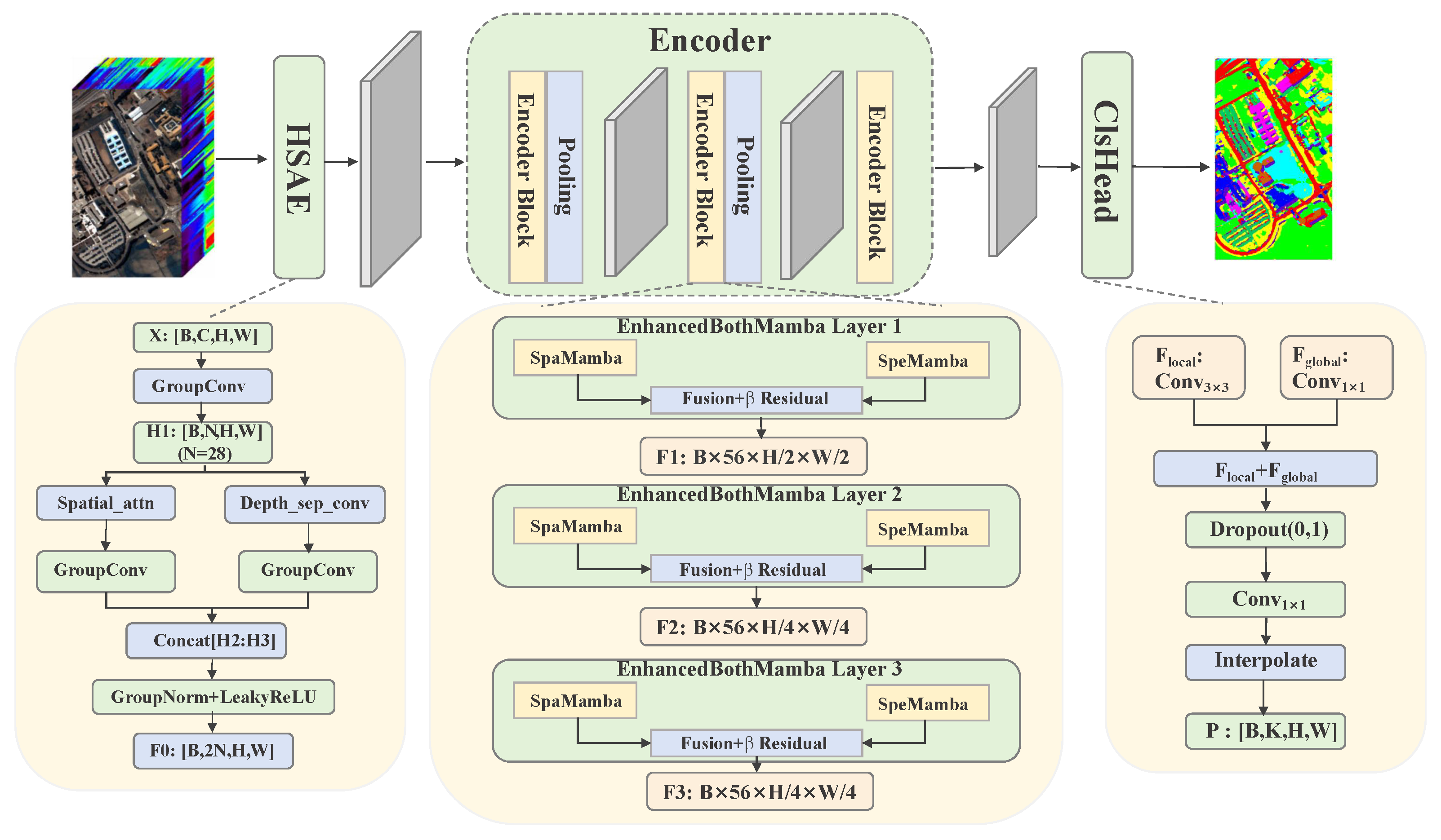
The overall architecture of the improved model (DFMamba) is illustrated in Figure 1. The model adopts an end-to-end pixel-wise classification design, which can directly process full hyperspectral images without pre-cropping or patch extraction. The model mainly consists of four core components:

• The Hyperspectral Spatial Attention Embed (HSAE), which replaces the simple patch embedding in the baseline model and achieves more efficient channel compression and feature extraction;
• The EnhancedBothMamba module, composed of the spatial Mamba (SpaMamba) and spectral Mamba (SpeMamba) branches, which separately model long-range dependencies in the spatial and spectral dimensions and integrate their outputs using softmax-normalized learnable global scalar weights together with a learnable residual scaling factor $\beta$;
• A multi-level feature extraction structure, which constructs a multi-scale feature pyramid via three EnhancedBothMamba layers and two average-pooling downsampling operations;
• The improved classification head (ClsHead), which adopts a multi-scale branch fusion strategy to fully exploit local and global features for pixel-wise classification.

The overall workflow is as follows: The input hyperspectral image $X\in {\mathbb{R}}^{B\times C\times H\times W}$, where B denotes batch size, C the number of spectral channels, and $H,W$ the spatial height and width, is processed by the HSAE module for channel compression and feature extraction, yielding the compressed feature representation ${\mathbf{F}}_0\in {\mathbb{R}}^{B\times 2N\times H\times W}$, where N denotes the channel compression factor. Following the sensitivity analysis presented in Section 4.2, we set $N=28$ as the default configuration because it provides the best balance between classification accuracy and computational efficiency. Subsequently, the features pass through three EnhancedBothMamba layers for spatial–spectral collaborative modeling, with average-pooling downsampling applied after the first two layers, forming a multi-scale feature set $\{{\mathbf{F}}_1,{\mathbf{F}}_2,{\mathbf{F}}_3\}$. Finally, the ClsHead module maps the multi-scale features to the class-logit space, producing the dense class-score tensor $\mathbf{P}\in {\mathbb{R}}^{B\times K\times H_c\times W_c}$, where K denotes the number of semantic classes and $H_c,W_c$ denote the spatial dimensions of the classification-head output. During training, the logits are resized to the spatial resolution of the ground-truth labels for loss computation. During inference, the logits are converted into class probabilities by the Softmax operation, and the final pixel-wise prediction is obtained by taking the $argmax$ over the class dimension. The network performs dense prediction over the entire hyperspectral image without patch cropping. Background or unlabeled pixels are not removed during forward inference. Instead, they are excluded only during optimization and quantitative evaluation using the predefined ignore mask.

3.2. Core Innovative Modules

3.2.1. Hyperspectral Spatial Attention Embed (HSAE)

The baseline MambaHSI compresses channels using a single $1\times 1$ convolution, which ignores the high-dimensional structure and redundancy inherent in hyperspectral data. The proposed HSAE addresses this issue via adaptive group convolution, depth-wise separable convolution, spatial attention, and feature concatenation with normalization.

Firstly, adaptive group convolution compresses the input feature $\mathbf{X}\in {\mathbb{R}}^{B\times C\times H\times W}$ from C channels to N channels, where the number of groups g is automatically set to the greatest common divisor of C and N. The resulting feature is computed as

$$H_1=GroupConv\left(\mathbf{X}\right),$$

(1)

where $H_1\in {\mathbb{R}}^{B\times N\times H\times W}$ denotes the output feature after the adaptive group convolution.

Secondly, a depth-wise separable convolution further extracts joint spatial–spectral features as follows:

$$H_2=\mathrm{Pointwise}\left(\mathrm{Depthwise}\left(H_1\right)\right).$$

(2)

Spatial attention is then introduced to enhance discriminative regions. First, a two-layer $1\times 1$ convolution generates the attention map A:

$$A=\sigma \left({\mathrm{Conv}}_{1\times 1}^2\left(\mathrm{ReLU}\left({\mathrm{Conv}}_{1\times 1}^1\left(H_1\right)\right)\right)\right),$$

(3)

where $\sigma$ denotes the sigmoid activation function. Then, the attention-weighted feature $H_3$ is obtained by element-wise multiplication of $H_1$ and A:

$$H_3=H_1\odot A,$$

(4)

where ⊙ represents element-wise multiplication. Finally, the features $H_2$ and $H_3$ are concatenated, and group normalization and LeakyReLU activation are performed to produce the final output $F_0$ of HSAE:

$$F_0=\mathrm{LeakyReLU}\left(\mathrm{GroupNorm}\left(\left[H_2;H_3\right]\right)\right),$$

(5)

where $[H_2;H_3]$ denotes the concatenation operation along the channel dimension.

This design effectively reduces spectral redundancy while preserving key discriminative information.

3.2.2. Learnable Weighted Fusion with Residual Scaling

The baseline BothMamba module combines the spatial and spectral features using simple addition or fixed weighting, which does not allow the relative contributions of the two branches to be optimized jointly with the network. In the final DFMamba architecture, the EnhancedBothMamba module adopts one specific fusion design: softmax-normalized learnable weighted fusion followed by a learnable residual scaling operation. Convolutional fusion and spatial-attention fusion are not simultaneously included in the final architecture; they are implemented only as alternative variants in the comparison experiments presented in Section 4.5.

Let ${\mathbf{X}}_{\mathrm{in}}\in {\mathbb{R}}^{B\times C\times H\times W}$ denote the input feature of an EnhancedBothMamba layer. The spatial and spectral branches produce ${\mathbf{F}}_{\mathrm{spa}}$ and ${\mathbf{F}}_{\mathrm{spe}}$, respectively. Two trainable scalar parameters, ${\alpha }_{\mathrm{spa}}$ and ${\alpha }_{\mathrm{spe}}$, are normalized using the Softmax function:

$$w_{\mathrm{spa}}={\displaystyle \frac{exp\left({\alpha }_{\mathrm{spa}}\right)}{exp\left({\alpha }_{\mathrm{spa}}\right)+exp\left({\alpha }_{\mathrm{spe}}\right)}},w_{\mathrm{spe}}={\displaystyle \frac{exp\left({\alpha }_{\mathrm{spe}}\right)}{exp\left({\alpha }_{\mathrm{spa}}\right)+exp\left({\alpha }_{\mathrm{spe}}\right)}}.$$

(6)

where $w_{\mathrm{spa}}$ and $w_{\mathrm{spe}}$ are the normalized fusion weights satisfying $w_{\mathrm{spa}}\ge 0$, $w_{\mathrm{spe}}\ge 0$, and $w_{\mathrm{spa}}+w_{\mathrm{spe}}=1$. The two branch features are then integrated as

$${\mathbf{F}}_{\mathrm{fusion}}=w_{\mathrm{spa}}{\mathbf{F}}_{\mathrm{spa}}+w_{\mathrm{spe}}{\mathbf{F}}_{\mathrm{spe}}.$$

(7)

A learnable residual scaling factor $\beta$ is introduced to control the contribution of the input shortcut. The final output of the EnhancedBothMamba module is uniformly defined as

$${\mathbf{F}}_{\mathrm{out}}=SiLU\left(w_{\mathrm{spa}}{\mathbf{F}}_{\mathrm{spa}}+w_{\mathrm{spe}}{\mathbf{F}}_{\mathrm{spe}}+\beta {\mathbf{X}}_{\mathrm{in}}\right).$$

(8)

In our implementation, ${\alpha }_{\mathrm{spa}}$, ${\alpha }_{\mathrm{spe}}$, and $\beta$ are global trainable scalar parameters. Consequently, the normalized weights $w_{\mathrm{spa}}$ and $w_{\mathrm{spe}}$ are shared across all samples in a batch, all feature channels, and all spatial positions. The weights are optimized jointly with the complete network during training, but they are not generated separately from each input sample. Therefore, the proposed fusion is neither sample-dependent, channel-wise, nor spatially varying. The term “learnable weighted fusion” is used throughout the revised manuscript to distinguish this mechanism from input-dependent dynamic gating.

The softmax normalization provides a constrained and interpretable balance between the two complementary branches, whereas the learnable residual factor $\beta$ allows the model to adjust the strength of the identity shortcut during end-to-end optimization. The same formulation in Equation (8) is used in all three EnhancedBothMamba layers of the final DFMamba architecture.

3.2.3. Improved Classification Head (ClsHead)

The improved classification head adopts a dual-branch structure. The local branch captures spatial details as follows:

$$F_{\mathrm{local}}=\mathrm{ReLU}6\left(\mathrm{BatchNorm}\left({\mathrm{Conv}}_{3\times 3}\left(F_{\mathrm{in}}\right)\right)\right),$$

(9)

where $F_{\mathrm{in}}$ denotes the input feature of the classification head. The global branch, on the other hand, aggregates channel-wise semantics as follows:

$$F_{\mathrm{global}}=\mathrm{ReLU}6\left(\mathrm{BatchNorm}\left({\mathrm{Conv}}_{1\times 1}\left(F_{\mathrm{in}}\right)\right)\right).$$

(10)

Unlike the preceding HSAE and EnhancedBothMamba modules, which focus on nonlinear feature extraction and long-range dependency modeling, ClsHead mainly serves as the final feature aggregation and prediction module. Therefore, ReLU6 is employed to constrain the activation range before the final linear classifier, reducing excessively large feature responses while maintaining computational simplicity. Since ClsHead contains only shallow convolutional transformations, preserving negative responses through LeakyReLU or using the smoother SiLU activation is less critical at this stage.

The fused feature is regularized by dropout, projected to the class-logit space through a $1\times 1$ convolution, and subsequently resized by bilinear interpolation to produce the class-score tensor:

$$\mathbf{P}=Interpolate\left({Conv}_{1\times 1}\left(Dropout\left(F_{\mathrm{local}}+F_{\mathrm{global}}\right)\right);H_c,W_c\right),$$

(11)

where Interpolate denotes bilinear interpolation, $(H_c,W_c)$ denotes the spatial resolution of the classification-head output, and the dropout rate is treated as a hyperparameter. The resulting tensor $\mathbf{P}\in {\mathbb{R}}^{B\times K\times H_c\times W_c}$ contains one class score for each semantic class. During training, the logits are resized to the spatial resolution of the ground-truth labels before loss computation. During inference, the final predicted label map is obtained by applying the Softmax function followed by the $argmax$ operation along the class dimension.

This dual-branch structure of ClsHead jointly leverages local detail and global semantics, resulting in superior classification accuracy.

3.3. Spatial–Spectral Dual-Branch Mamba Module

The BothMamba module serves as the central computational unit, consisting of SpaMamba for spatial modeling and SpeMamba for spectral modeling. For SpaMamba, the input feature map is reshaped into a spatial sequence, which is expressed as

$$F_{\mathrm{seq}}=\mathrm{Reshape}\left(F\right)\in {\mathbb{R}}^{1\times (H\times W)\times C},$$

(12)

and Mamba is then applied to model long-range spatial dependencies:

$$F_{\mathrm{spa}}=\mathrm{Mamba}\left(F_{\mathrm{seq}}\right).$$

(13)

After reshaping and activation, the spatial feature is updated as follows:

$$F_{\mathrm{spa}}=\mathrm{SiLU}\left(\mathrm{GroupNorm}\left(\mathrm{Reshape}\left(F_{\mathrm{spa}}\right)\right)\right).$$

(14)

For spectral modeling, the channels are divided into T spectral groups, each fed into a Mamba block, which is defined as follows:

$$F_{\mathrm{spe}}=\mathrm{Mamba}\left(\mathrm{Group}\left(F\right)\right),$$

(15)

where $\mathrm{Group}(·)$ denotes the spectral grouping operation that partitions the C channels into T non-overlapping groups. The resulting spectral feature is then reshaped, normalized, and activated:

$$F_{\mathrm{spe}}=\mathrm{SiLU}\left(\mathrm{GroupNorm}\left(\mathrm{Reshape}\left(F_{\mathrm{spe}}\right)\right)\right).$$

(16)

After the two branches produce ${\mathbf{F}}_{\mathrm{spa}}$ and ${\mathbf{F}}_{\mathrm{spe}}$, their outputs are integrated using the unified learnable weighted fusion mechanism defined in Section 3.2.2. Specifically, the branch coefficients are obtained by applying Softmax normalization to two global trainable scalar parameters, and the input feature is incorporated through the learnable residual scaling factor $\beta$. Therefore, the output of the complete EnhancedBothMamba module is computed using Equation (8). No separate fusion equation or additional parameterization is used in this module.

The parallel spatial and spectral branches capture complementary long-range dependencies, while the unified fusion operation learns a stable global balance between their representations. This design achieves deep spatial–spectral coupling while retaining the linear-complexity advantage of the Mamba architecture. The complete forward propagation pseudocode of the proposed EnhancedBothMamba layer is presented in

Table 2. Pseudocode for the forward propagation of an EnhancedBothMamba layer.

Step	Operation
Input	${\mathbf{X}}_{\mathrm{in}}\in {\mathbb{R}}^{B\times C\times H\times W}$
1	${\mathbf{F}}_{\mathrm{spa}}\leftarrow SpaMamba\left({\mathbf{X}}_{\mathrm{in}}\right)$
2	${\mathbf{F}}_{\mathrm{spe}}\leftarrow SpeMamba\left({\mathbf{X}}_{\mathrm{in}}\right)$
3	$[w_{\mathrm{spa}},w_{\mathrm{spe}}]\leftarrow Softmax\left([{\alpha }_{\mathrm{spa}},{\alpha }_{\mathrm{spe}}]\right)$
4	${\mathbf{F}}_{\mathrm{fusion}}\leftarrow w_{\mathrm{spa}}{\mathbf{F}}_{\mathrm{spa}}+w_{\mathrm{spe}}{\mathbf{F}}_{\mathrm{spe}}$
5	${\mathbf{F}}_{\mathrm{out}}\leftarrow SiLU({\mathbf{F}}_{\mathrm{fusion}}+\beta {\mathbf{X}}_{\mathrm{in}})$
Output	${\mathbf{F}}_{\mathrm{out}}$

${\alpha }_{\mathrm{spa}}$, ${\alpha }_{\mathrm{spe}}$, and $\beta$ are global trainable scalar parameters shared across the sample, channel, and spatial dimensions.

.

3.4. Multi-Level Feature Extraction Structure

The framework employs three EnhancedBothMamba layers and two average-pooling operations to construct a multi-scale feature pyramid. All three EnhancedBothMamba layers use the same learnable weighted fusion and $\beta$-scaled residual formulation defined in Equation (8); each layer has its own trainable fusion and residual parameters.

The output of the first layer is expressed as follows:

$$F_1=\mathrm{AvgPool}\left({\mathrm{EnhancedBothMamba}}_1\left(F_0\right)\right),$$

(17)

where $F_0$ denotes the input feature of the multi-scale feature pyramid (i.e., the output of the preceding module), and ${\mathrm{EnhancedBothMamba}}_1$ represents the first layer of the EnhancedBothMamba module. The output of the second layer is formulated as follows:

$$F_2=\mathrm{AvgPool}\left({\mathrm{EnhancedBothMamba}}_2\left(F_1\right)\right),$$

(18)

where ${\mathrm{EnhancedBothMamba}}_2$ denotes the second layer of the EnhancedBothMamba module. The output of the third layer is defined as follows:

$$F_3={\mathrm{EnhancedBothMamba}}_3\left(F_2\right),$$

(19)

where ${\mathrm{EnhancedBothMamba}}_3$ is the third layer of the EnhancedBothMamba module.

By progressively downsampling via average-pooling operations, the receptive field is enlarged, enabling hierarchical semantic abstraction from local to global representations. This multi-scale feature pyramid structure achieves a balance between computational efficiency and feature expressiveness, significantly enhancing the capability of multi-scale feature modeling.

3.5. Loss Function

This work adopts the cross-entropy loss function for end-to-end pixel-wise classification. The classification head outputs the class-logit tensor $\mathbf{P}\in {\mathbb{R}}^{B\times K\times H_c\times W_c}$. Before loss computation, the logits are resized to match the spatial resolution of the ground-truth labels using bilinear interpolation,

$$\mathbf{Z}=Interpolate(\mathbf{P};H,W),$$

(20)

where $\mathbf{Z}\in {\mathbb{R}}^{B\times K\times H\times W}$.

The corresponding class probabilities are defined as

$${\widehat{P}}_{b,k,i,j}={\displaystyle \frac{exp\left(Z_{b,k,i,j}\right)}{{\sum }_{c=0}^{K-1}exp\left(Z_{b,c,i,j}\right)}},$$

(21)

where $\widehat{\mathbf{P}}\in {[0,1]}^{B\times K\times H\times W}$.

The ground-truth labels are represented by the integer-valued label map

$$\mathbf{Y}\in {\{-1,0,\dots ,K-1\}}^{B\times H\times W},$$

where $-1$ denotes ignored pixels (background or unlabeled regions).

Only valid labeled pixels participate in optimization. Accordingly, the cross-entropy loss is computed as

$${\mathcal{L}}_{\mathrm{CE}}=-{\displaystyle \frac{1}{N_{\mathrm{valid}}}}\sum _{b,i,j}{M}_{b,i,j}log{\widehat{P}}_{b,Y_{b,i,j},i,j},$$

(22)

where

$$M_{b,i,j}=\left\{\begin{array}{cc}1,\hfill & Y_{b,i,j}\ne -1,\hfill \\ 0,\hfill & Y_{b,i,j}=-1,\hfill \end{array}\right.$$

and

$$N_{\mathrm{valid}}=\sum _{b,i,j}{M}_{b,i,j}$$

denotes the number of valid labeled pixels.

In the implementation, the resized logits $\mathbf{Z}$ are directly passed to the PyTorch (version 1.13.1) cross-entropy loss function, which internally performs the log-Softmax operation. Therefore, pixels labeled as $-1$ do not contribute to either the loss value or the gradient computation.

End-to-end training jointly updates the parameters of the HSAE module, the multi-level feature extraction structure, the EnhancedBothMamba module, and the ClsHead. The Adam optimizer is adopted together with learning-rate decay, early stopping, and data augmentation to improve training stability and model generalization.

4. Experiments

4.1. Experimental Setup

4.1.1. Datasets

To comprehensively evaluate the proposed DFMamba model, experiments were conducted on four hyperspectral remote sensing datasets: HanChuan, HongHu, Houston, and Pavia University (UP). These datasets represent diverse Earth observation scenarios (agricultural monitoring, urban land cover analysis, and ecosystem mapping) and serve as widely adopted benchmarks in hyperspectral remote sensing studies. Thus, they are able to provide a thorough validation of the model’s generalization and robustness.

The Pavia University dataset was acquired by the ROSIS sensor and contains 610 × 340 pixels and 103 valid spectral bands covering nine typical urban land cover classes, including asphalt, grass, gravel, trees, bare soil, bricks, and shadows, with a spatial resolution of 1.3 m. The HanChuan dataset was collected by a Headwall Nano-Hyperspec sensor mounted on an unmanned aerial vehicle on 17 June 2016, in Hanchuan, China. It contains 1217 × 307 pixels and 274 spectral bands (400–1000 nm) covering 16 land cover classes, including multiple crop types and mixed urban–rural regions, with a spatial resolution of 0.109 m. The HongHu dataset, also acquired by the Headwall Nano-Hyperspec sensor, on 20 November 2017, in Honghu, China, has an image size of 940 × 475, 270 spectral bands, and 22 land cover classes, mainly farmland, wetlands, buildings, and water bodies, with a spatial resolution of 0.043 m. The Houston dataset was collected by the ITRES CASI 1500 sensor in the University of Houston area, Texas, USA, and comprises 349 × 1905 pixels and 144 bands (380–1050 nm) with 15 land cover classes and a spatial resolution of approximately 2.5 m. The significant differences in spatial and spectral characteristics across these datasets allow a thorough evaluation of model robustness and generalization capability.

Prior to training and evaluation, the official ground-truth annotations provided with each dataset were adopted. Pixels annotated as background or unlabeled regions were assigned an ignore label and therefore did not contribute to the loss computation or quantitative evaluation. During both training and inference, however, the complete hyperspectral image was processed in an end-to-end manner without removing background regions or cropping image patches. This strategy preserves the spatial continuity of the scene while ensuring that only valid semantic classes contribute to model optimization and accuracy assessment.

4.1.2. Evaluation Metrics and Comparison Methods

First, model performance was quantitatively evaluated using Overall Accuracy (OA), Average Accuracy (AA), and the Kappa coefficient. OA reflects the overall classification accuracy, AA measures the average classification performance across classes, and the Kappa coefficient eliminates the influence of random agreement, providing a more objective assessment of model performance.

To demonstrate the superiority of DFMamba, several representative comparison methods were selected, including traditional machine learning approaches (SVM, RF), graph convolution-based methods (DMSGer, GiGCN), convolutional neural network-based methods covering different convolution paradigms (2D convolution-based FullyContNet and CLOLN, hybrid 2D-3D convolution-based HybridSN, 3D residual convolution-based SSRN), and Transformer-based methods (SpectralFormer, GSC-ViT). To guarantee a fair comparison, all comparative models follow the unified pixel sampling rule: 30 training pixels and 10 validation pixels are randomly extracted from each land-cover class, all leftover labeled pixels form the test set, and the whole sampling procedure is reproduced 10 times with different random seeds to obtain stable statistical results. These methods cover the main development pathways in hyperspectral image classification from traditional machine learning to deep learning and state-space models, thus comprehensively reflecting the differences in spatial–spectral feature modeling.

4.1.3. Implementation Details and Sampling Strategy

All experiments were implemented in the PyTorch framework on a workstation equipped with an NVIDIA RTX 3090 GPU (24 GB VRAM), an Intel Xeon Gold 6226R CPU, and 256 GB RAM. To ensure a strictly fair comparison, the sampling configuration strictly follows the baseline MambaHSI [26]: 30 training samples and 10 validation samples per class, with the remaining pixels used for testing. Addressing the potential sampling bias inherent in such few-shot settings, the specific 30 training samples and 10 validation samples for each class were independently and randomly redrawn for every single one of the 10 experimental runs. This rigorous cross-validation strategy, rather than a one-time split, guarantees that the reported averages and the low standard deviations reflect the model’s true learning capability under extreme label scarcity, rather than artifacts of a favorable data split. The model was optimized using the Adam optimizer with an initial learning rate of 0.0003 and a batch size of 1. Since the proposed framework adopts an end-to-end full-scene input strategy, each training sample corresponds to an entire hyperspectral image. Owing to the high memory consumption of full-scene feature extraction on the GPU, the batch size is set to be 1 to satisfy the available GPU memory constraints.The Mamba module parameters were set to follow the original reference [26] to ensure fair comparison. Ground-truth pixels labeled as background or unlabeled regions were assigned an ignore label during training. Consequently, they were excluded from loss computation and quantitative evaluation but remained in the input image during the forward pass, enabling end-to-end dense prediction over the complete hyperspectral scene.Unless otherwise specified, the channel compression factor of the proposed HSAE module was set to $N=28$ throughout all experiments. The rationale for selecting this value, together with its sensitivity analysis and computational complexity comparison, is presented in Section 4.2.

4.2. Channel Compression Factor Selection and Sensitivity Analysis

The proposed HSAE module introduces the channel compression factor N, which determines the feature dimensionality before the spatial–spectral Mamba encoder. Since N directly influences both feature representation capability and computational complexity, its value was determined through sensitivity analysis rather than exhaustive grid search. A smaller N may excessively compress spectral information, whereas a larger N increases computational cost without necessarily providing consistent accuracy improvements. Therefore, both classification performance and computational efficiency should be considered when selecting N.

To investigate the influence of N, four representative settings, $N=\{16,28,32,48\}$, were evaluated on the UP, HanChuan, HongHu, and Houston datasets. The corresponding OA and AA results are reported in

Table 3. Sensitivity analysis of the channel compression factor N on classification accuracy (%).

N	UP		HanChuan		HongHu		Houston
	OA	AA	OA	AA	OA	AA	OA	AA
16	$95.07\pm 1.52$	$96.35\pm 0.97$	$80.70\pm 3.85$	$81.77\pm 1.76$	$77.26\pm 6.44$	$88.41\pm 1.12$	$90.82\pm 2.34$	$92.21\pm 1.89$
28	$\mathbf{97.41}\pm \mathbf{0.74}$	$\mathbf{97.74}\pm \mathbf{0.45}$	$92.25\pm 1.39$	$91.79\pm 1.14$	$95.12\pm 1.12$	$\mathbf{95.59}\pm \mathbf{0.48}$	$\mathbf{94.98}\pm \mathbf{0.89}$	$\mathbf{95.73}\pm \mathbf{0.80}$
32	$96.98\pm 2.20$	$97.32\pm 1.75$	$\mathbf{93.20}\pm \mathbf{0.84}$	$92.09\pm 0.71$	$94.75\pm 0.59$	$95.14\pm 0.58$	$94.16\pm 1.10$	$94.95\pm 0.86$
48	$96.72\pm 1.80$	$97.09\pm 0.73$	$92.71\pm 0.55$	$\mathbf{92.33}\pm \mathbf{0.69}$	$\mathbf{95.29}\pm \mathbf{0.64}$	$95.57\pm 0.17$	$93.63\pm 2.43$	$94.52\pm 2.18$

Note: Bold indicates the selected final model ($N=28$).

. The highest accuracy varies across datasets and evaluation metrics, indicating that no single value of N is uniformly optimal. To provide an overall comparison, an average-rank analysis was additionally conducted. For each dataset, the four settings were ranked separately according to OA and AA, and the resulting eight ranks were averaged to obtain the mean accuracy rank. As summarized in

Table 4. Cross-dataset mean accuracy rank and average computational complexity under different channel compression factors.

N	Average Params (K)	Average FLOPs (G)	Mean Accuracy Rank
16	67.68	11.16	4.000
28	$\mathbf{144.13}$	$\mathbf{25.01}$	$\mathbf{1.625}$
32	179.77	30.20	2.125
48	318.50	56.28	2.250

Note: For each dataset, the four settings are ranked separately according to OA and AA, where rank 1 denotes the highest accuracy. The mean accuracy rank is obtained by averaging the resulting eight ranks over the four datasets and two evaluation metrics. The parameter count and FLOPs are not included in the rank calculation and are reported separately as computational complexity indicators. A lower mean accuracy rank indicates better aggregate classification performance. Bold indicates the selected final model ($N=28$).

, $N=28$ achieves the lowest mean accuracy rank (1.625), followed by $N=32$ (2.125), $N=48$ (2.250), and $N=16$ (4.000), suggesting comparatively consistent classification performance across the evaluated datasets. The mean accuracy rank is calculated from the OA and AA rankings, while parameter count and FLOPs are reported separately as computational complexity measures.

Table 4 further shows that increasing N from 28 to 32 raises the average parameter count from 144.13 K to 179.77 K and the average FLOPs from 25.01 G to 30.20 G, corresponding to increases of approximately 24.7% and 20.8%, respectively. Increasing N to 48 further raises the average parameter count to 318.50 K and the average FLOPs to 56.28 G, representing increases of approximately 121.0% and 125.0%, respectively. Although $N=16$ requires the lowest computational cost, it exhibits the poorest overall classification performance. In contrast, the substantially higher computational cost of $N=32$ and $N=48$ does not lead to a better mean accuracy rank than $N=28$.

Therefore, although $N=28$ is not the best-performing setting for every individual dataset or evaluation metric, it achieves the lowest cross-dataset mean accuracy rank while requiring substantially lower computational cost than the larger settings. Accordingly, $N=28$ was adopted as the default channel compression factor in all subsequent experiments.

4.3. Comparison with State-of-the-Art Methods

As shown in

Table 5. Comparison of the classification accuracy of different methods on representative datasets.

Method	Dataset	OA (%)	AA (%)	Kappa (%)
DFMamba (Ours)	UP	$97.41\pm 0.74$	$97.74\pm 0.45$	$97.00\pm 2.11$
MambaHSI [26]	UP	$95.74\pm 0.90$	$95.86\pm 1.11$	$95.00\pm 2.24$
SVM [5]	UP	$71.31\pm 3.15$	$71.98\pm 1.39$	$63.96\pm 3.19$
RF [6]	UP	$70.68\pm 2.61$	$71.14\pm 1.61$	$63.13\pm 2.81$
DMSGer [47]	UP	$89.55\pm 1.22$	$93.15\pm 0.70$	$86.49\pm 1.54$
GiGCN [46]	UP	$94.47\pm 0.97$	$92.93\pm 1.07$	$92.67\pm 1.26$
FullyContNet [64]	UP	$91.31\pm 9.36$	$93.41\pm 6.57$	$93.12\pm 5.19$
CLOLN [65]	UP	$94.97\pm 1.43$	$93.53\pm 1.59$	$93.38\pm 1.84$
SpectralFormer [22]	UP	$91.10\pm 2.60$	$79.93\pm 2.67$	$77.40\pm 4.41$
GSC-ViT [42]	UP	$92.65\pm 2.30$	$91.89\pm 1.73$	$90.38\pm 2.95$
HybridSN [14]	UP	$90.20\pm 3.74$	$91.65\pm 1.78$	$87.27\pm 4.70$
SSRN [11]	UP	$88.33\pm 2.94$	$89.43\pm 1.70$	$84.79\pm 3.66$
DFMamba (Ours)	HanChuan	$92.25\pm 1.39$	$91.79\pm 1.14$	$90.93\pm 1.82$
MambaHSI [26]	HanChuan	$90.21\pm 1.67$	$89.20\pm 1.36$	$89.07\pm 2.31$
SVM [5]	HanChuan	$60.98\pm 1.35$	$51.48\pm 1.46$	$56.00\pm 1.49$
RF [6]	HanChuan	$64.09\pm 1.78$	$48.89\pm 1.15$	$59.05\pm 1.86$
DMSGer [47]	HanChuan	$84.39\pm 1.83$	$88.26\pm 0.89$	$82.01\pm 2.02$
GiGCN [46]	HanChuan	$86.78\pm 1.43$	$76.47\pm 1.62$	$84.64\pm 1.62$
FullyContNet [64]	HanChuan	$84.88\pm 3.02$	$77.42\pm 3.61$	$75.80\pm 4.70$
CLOLN [65]	HanChuan	$85.14\pm 2.93$	$76.13\pm 3.26$	$82.75\pm 3.31$
SpectralFormer [22]	HanChuan	$82.99\pm 2.31$	$71.13\pm 2.56$	$80.29\pm 2.61$
GSC-ViT [42]	HanChuan	$83.14\pm 3.96$	$73.97\pm 2.06$	$80.57\pm 4.33$
HybridSN [14]	HanChuan	$88.25\pm 1.31$	$88.00\pm 0.72$	$86.35\pm 1.50$
SSRN [11]	HanChuan	$90.43\pm 0.92$	$89.88\pm 1.05$	$88.86\pm 1.07$
DFMamba (Ours)	HongHu	$95.12\pm 1.12$	$95.59\pm 0.48$	$95.00\pm 1.38$
MambaHSI [26]	HongHu	$94.58\pm 1.01$	$94.77\pm 0.61$	$94.00\pm 1.88$
SVM [5]	HongHu	$68.77\pm 1.27$	$54.50\pm 0.41$	$62.71\pm 1.28$
RF [6]	HongHu	$59.85\pm 2.13$	$48.08\pm 1.05$	$53.22\pm 1.95$
DMSGer [47]	HongHu	$75.43\pm 4.34$	$90.73\pm 0.92$	$71.59\pm 4.32$
GiGCN [46]	HongHu	$87.22\pm 0.60$	$74.08\pm 1.50$	$83.95\pm 0.73$
FullyContNet [64]	HongHu	$92.19\pm 1.35$	$93.47\pm 0.48$	$93.86\pm 1.54$
CLOLN [65]	HongHu	$87.93\pm 2.11$	$77.60\pm 2.25$	$85.06\pm 2.49$
SpectralFormer [22]	HongHu	$86.04\pm 2.83$	$73.17\pm 2.45$	$82.72\pm 3.22$
GSC-ViT [42]	HongHu	$86.18\pm 1.86$	$74.74\pm 1.64$	$82.93\pm 2.16$
HybridSN [14]	HongHu	$88.89\pm 1.16$	$88.45\pm 1.29$	$86.10\pm 1.42$
SSRN [11]	HongHu	$92.53\pm 0.99$	$92.54\pm 0.87$	$90.64\pm 1.23$
DFMamba (Ours)	Houston	$94.98\pm 0.89$	$95.73\pm 0.8$	$94.79\pm 2.1$
MambaHSI [26]	Houston	$94.46\pm 0.83$	$95.34\pm 0.78$	$94.21\pm 1.93$
SVM [5]	Houston	$79.63\pm 1.04$	$80.70\pm 1.03$	$77.97\pm 1.12$
RF [6]	Houston	$78.95\pm 0.90$	$79.24\pm 0.83$	$77.25\pm 0.98$
DMSGer [47]	Houston	$90.36\pm 1.29$	$92.17\pm 1.07$	$89.58\pm 1.39$
GiGCN [46]	Houston	$88.13\pm 2.26$	$89.85\pm 1.91$	$87.16\pm 2.44$
FullyContNet [64]	Houston	$89.79\pm 4.20$	$91.35\pm 3.55$	$90.64\pm 4.68$
CLOLN [65]	Houston	$90.31\pm 1.73$	$91.80\pm 1.46$	$89.52\pm 1.87$
SpectralFormer [22]	Houston	$89.13\pm 2.12$	$89.89\pm 1.74$	$88.24\pm 2.29$
GSC-ViT [42]	Houston	$91.85\pm 1.05$	$92.97\pm 0.92$	$91.18\pm 1.14$
HybridSN [14]	Houston	$91.78\pm 1.36$	$93.14\pm 1.16$	$91.11\pm 1.47$
SSRN [11]	Houston	$88.58\pm 1.58$	$90.33\pm 1.55$	$87.65\pm 1.71$

, the proposed DFMamba method achieved the best or near-best classification performance on all four datasets. On the UP dataset, our method reached an OA of 97.41%, which is 1.67 percentage points higher than the baseline MambaHSI and 2.44, 2.94, 4.76, 6.31, 7.21, and 9.08 percentage points higher than other state-of-the-art methods CLOLN (94.97%), GiGCN (94.47%), GSC-ViT (92.65%), SpectralFormer (91.10%), HybridSN (90.20%), and SSRN (88.33%), respectively. In terms of AA and the Kappa coefficient, our method also performed excellently, achieving 97.74% and 97.00%, with higher mean values than other compared methods. Traditional machine learning methods SVM and RF achieved relatively poor performance on the UP dataset, with OAs of 71.31% and 70.68%, respectively, confirming the advantage of deep learning-based Mamba architectures for hyperspectral image classification even under the constraint of only 30 training samples per class.

On the HanChuan dataset, DFMamba also demonstrated outstanding performance, with an OA of 92.25%. This represents an improvement of 2.04 percentage points over the baseline MambaHSI, and improvements of 1.82, 5.47, 4.00, 7.11, 7.86, and 9.26 percentage points over SSRN (90.43%), GiGCN (86.78%), HybridSN (88.25%), CLOLN (85.14%), DMSGer (84.39%), and SpectralFormer (82.99%), respectively. The HanChuan dataset has a notably large spatial size (1217 × 307 pixels) and many spectral bands (274). Crucially, even with such a sparse training set covering a wide spatial extent, DFMamba maintains robust feature extraction, validating its effectiveness for large-scale hyperspectral images where dense annotation is impractical.

On the HongHu dataset, our method achieved 95.12%OA, which was higher than that of the baseline MambaHSI by 0.54 percentage points and achieving higher mean OA than FullyContNet (92.19%), CLOLN (87.93%), GiGCN (87.22%), HybridSN (88.89%), and SSRN (92.53%). The HongHu dataset contains 22 land cover classes, the most among the four datasets, demonstrating the strong capability of our method for multi-class classification tasks.

On the Houston dataset, DFMamba reached 94.98%OA, an improvement of 0.52 percentage points over the baseline MambaHSI, and improvements of 3.13, 3.20, 4.62, 4.67, 5.85, and 6.40 percentage points over GSC-ViT (91.85%), HybridSN (91.78%), DMSGer (90.36%), CLOLN (90.31%), SpectralFormer (89.13%), and SSRN (88.58%), respectively. The Houston dataset has a large spatial size (349 × 1905 pixels), and thus our method’s performance demonstrates its capability to handle large-scale images.

From a stability perspective, our method achieved low standard deviations on all datasets, e.g., 0.74%OA on UP and 0.89%on Houston, indicating good stability and reproducibility. In contrast, some methods showed significant performance fluctuations, such as FullyContNet, which exhibited a standard deviation of 9.36%on the UP dataset, and HybridSN, which showed a standard deviation of 1.31%on the HanChuan dataset. The relatively small standard deviations indicate limited run-to-run variability under the adopted sampling protocol.

Overall, across the four datasets, DFMamba achieved an average OA improvement of 25–30 percentage points over traditional machine learning methods (SVM, RF), 5–8 percentage points over graph convolution-based methods (DMSGer, GiGCN), 3–6 percentage points over Transformer-based methods (SpectralFormer, GSC-ViT), and 2–5 percentage points over contrastive learning-based methods (FullyContNet, CLOLN). Furthermore, DFMamba consistently outperformed 3D-CNN-based approaches (HybridSN and SSRN) by margins ranging from 3% to 9%. These results highlight that the linear sequential modeling of DFMamba is inherently more effective at extracting discriminative features from limited training pixels than local cubic convolutions or quadratic attention mechanisms. These improvements are mainly attributable to the following key innovations: the HSAE module performs more effective channel compression and feature extraction via adaptive grouped convolution, depth-wise separable convolution, and spatial attention; the EnhancedBothMamba module adaptively integrates spatial–spectral features through spatial attention fusion; the multi-scale progressive architecture captures features hierarchically from local details to global semantics; and the improved ClsHead module fuses local and global features to achieve fine-grained pixel-level classification. Together, these innovations enable DFMamba to significantly enhance classification accuracy and robustness while maintaining computational efficiency.

4.4. Ablation Study

To comprehensively investigate the contribution of each component in DFMamba, ablation experiments were conducted from three perspectives: overall component analysis, internal component analysis of HSAE, and branch analysis of ClsHead. It should be noted that the SpaMamba and SpeMamba branches are directly inherited from the baseline MambaHSI without architectural modification. Therefore, their individual contributions have already been investigated in the original MambaHSI framework and are not repeated in this work. Instead, this study focuses on the newly introduced components of DFMamba, including the HSAE module, the dual-branch ClsHead, and the proposed fusion strategy. The effectiveness of the EnhancedBothMamba fusion mechanism, including the learnable fusion strategy and residual scaling factor $\beta$, is further analyzed in the Fusion Mechanism Comparison section.

Firstly, the contributions of the major newly introduced components were evaluated by removing HSAE and ClsHead separately. As shown in

Table 6. Performance analysis of DFMamba and its variants on multiple datasets.

Dataset	HSAE	ClsHead	OA (%)	AA (%)	Kappa (%)	$\Delta$OA	$\Delta$AA	$\Delta$Kappa
HanChuan	✓	✓	$92.25\pm 1.39$	$91.79\pm 1.14$	$90.93\pm 1.82$	–	–	–
	×	✓	$89.55\pm 2.70$	$90.18\pm 1.52$	$89.47\pm 2.61$	$-2.70$	$-1.61$	$-1.46$
	✓	×	$80.92\pm 3.22$	$83.39\pm 1.41$	$80.33\pm 3.10$	$-11.33$	$-8.40$	$-10.60$
HongHu	✓	✓	$95.12\pm 1.12$	$95.59\pm 0.48$	$95.00\pm 1.38$	–	–	–
	×	✓	$94.67\pm 0.54$	$95.26\pm 0.20$	$94.21\pm 1.18$	$-0.45$	$-0.33$	$-0.79$
	✓	×	$75.60\pm 4.52$	$89.52\pm 3.62$	$88.00\pm 3.18$	$-19.52$	$-6.07$	$-7.00$
Houston	✓	✓	$94.98\pm 0.89$	$95.73\pm 0.80$	$94.79\pm 2.10$	–	–	–
	×	✓	$94.45\pm 1.03$	$94.53\pm 0.90$	$93.57\pm 6.40$	$-0.53$	$-1.20$	$-1.22$
	✓	×	$92.06\pm 1.00$	$93.39\pm 0.85$	$92.57\pm 2.12$	$-2.92$	$-2.34$	$-2.22$
UP	✓	✓	$97.41\pm 0.74$	$97.74\pm 0.45$	$97.00\pm 2.11$	–	–	–
	×	✓	$96.49\pm 1.17$	$97.44\pm 0.83$	$97.05\pm 2.03$	$-0.92$	$-0.30$	$+0.05$
	✓	×	$91.07\pm 3.20$	$94.25\pm 3.29$	$91.63\pm 5.89$	$-6.34$	$-3.49$	$-5.37$

, removing either HSAE or ClsHead resulted in performance degradation, verifying the effectiveness of these modules in the proposed framework.

On the HanChuan dataset, removing HSAE and ClsHead resulted in OA decreases of 2.70 and 11.33 percentage points, respectively. In particular, removing ClsHead caused a substantial decrease of 10.60 percentage points in the Kappa coefficient, indicating that the proposed classification head plays an important role in improving classification consistency.

On the HongHu dataset, removing HSAE caused a relatively small OA decrease of 0.45 percentage points, whereas removing ClsHead resulted in a significant OA reduction of 19.52 percentage points. Since HongHu contains 22 land-cover categories, this large performance degradation demonstrates the importance of the dual-branch ClsHead in distinguishing complex categories. The full DFMamba achieves the best performance by jointly exploiting feature representation and classification refinement.

On the Houston dataset, removing ClsHead reduced the OA by 2.92 percentage points. Although the Kappa standard deviation slightly increased from 2.10% to 2.12%, this difference is very small and mainly reflects run-to-run variability rather than a meaningful stability change.

On the UP dataset, removing HSAE decreased the OA by 0.92 percentage points, while removing ClsHead resulted in a larger degradation of 6.34 percentage points. These results indicate that ClsHead has a more significant influence on classification performance, whereas HSAE mainly contributes to discriminative feature representation.

The computational efficiency comparison is presented in

Table 7. Comparison of computational efficiency of DFMamba and its variants on four datasets.

Dataset	HSAE	ClsHead	Train Time (s)	Test Time (ms)	Train Inc. (%)	Test Inc. (%)
HanChuan	✓	✓	$223.40\pm 0.94$	$307.99\pm 0.63$	–	–
	×	✓	$281.08\pm 13.74$	$360.37\pm 3.11$	$+25.82$	$+16.99$
	✓	×	$228.57\pm 1.73$	$322.41\pm 0.35$	$+2.31$	$+4.68$
HongHu	✓	✓	$248.86\pm 0.94$	$357.79\pm 0.84$	–	–
	×	✓	$277.99\pm 46.54$	$371.62\pm 3.51$	$+11.71$	$+3.86$
	✓	×	$252.60\pm 0.60$	$369.50\pm 0.25$	$+1.50$	$+3.27$
Houston	✓	✓	$386.41\pm 0.97$	$536.79\pm 0.41$	–	–
	×	✓	$531.36\pm 58.32$	$694.84\pm 8.88$	$+37.51$	$+29.44$
	✓	×	$382.94\pm 1.08$	$538.12\pm 0.32$	$-0.90$	$+0.25$
UP	✓	✓	$126.18\pm 0.42$	$200.08\pm 1.01$	–	–
	×	✓	$130.30\pm 10.68$	$184.96\pm 1.57$	$+3.27$	$-7.56$
	✓	×	$128.66\pm 1.60$	$197.37\pm 0.20$	$+1.97$	$-1.35$

. Removing HSAE generally increases the overall training and testing time on most datasets, indicating that the proposed HSAE design provides an effective balance between feature representation and computational efficiency. In contrast, removing ClsHead causes only marginal runtime variations. For example, on the Houston dataset, removing ClsHead slightly increases the testing time by 0.25%. This counter-intuitive variation does not indicate that ClsHead introduces additional efficiency advantages, but is mainly caused by runtime fluctuations related to GPU execution scheduling, memory access patterns, and measurement noise. Therefore, the computational overhead introduced by ClsHead is considered negligible.

To further analyze the internal design of HSAE, several simplified variants were constructed by retaining only one feature extraction branch or replacing the grouped convolution operation. The results are reported in

Table 8. Ablation study on the Hyperspectral Spatial Attention Embed (HSAE).

Dataset	Configuration	OA (%)	AA (%)	Kappa (%)
Houston	Full HSAE	$94.98\pm 0.89$	$95.73\pm 0.80$	$94.79\pm 2.10$
	Depth-wise Branch Only	$94.33\pm 0.93$	$95.17\pm 0.82$	$94.57\pm 1.16$
	Attention Branch Only	$94.15\pm 0.89$	$95.04\pm 0.77$	$94.07\pm 1.63$
	w/o Group	$94.60\pm 0.89$	$95.43\pm 0.81$	$94.07\pm 1.60$
HongHu	Full HSAE	$95.12\pm 1.12$	$95.59\pm 0.48$	$95.00\pm 1.38$
	Depth-wise Branch Only	$94.37\pm 1.22$	$94.77\pm 0.76$	$93.95\pm 1.93$
	Attention Branch Only	$94.68\pm 0.56$	$94.88\pm 0.51$	$94.10\pm 1.94$
	w/o GroupConv	$94.46\pm 1.14$	$94.98\pm 0.45$	$94.62\pm 1.22$
HanChuan	Full HSAE	$92.25\pm 1.39$	$91.79\pm 1.14$	$90.93\pm 1.82$
	Depth-wise Branch Only	$90.88\pm 1.28$	$90.19\pm 1.32$	$90.67\pm 1.76$
	Attention Branch Only	$90.63\pm 1.63$	$89.28\pm 1.01$	$88.60\pm 2.20$
	w/o GroupConv	$90.78\pm 1.24$	$89.90\pm 1.12$	$88.33\pm 1.91$
UP	Full HSAE	$97.41\pm 0.74$	$97.74\pm 0.45$	$97.00\pm 2.11$
	Depth-wise Branch Only	$96.44\pm 1.10$	$97.13\pm 0.68$	$96.62\pm 1.62$
	Attention Branch Only	$96.28\pm 1.29$	$97.22\pm 0.76$	$97.13\pm 2.17$
	w/o GroupConv	$96.61\pm 1.33$	$97.23\pm 0.63$	$96.88\pm 1.70$

.

The complete HSAE consistently achieves the highest classification accuracy across all four datasets, demonstrating that the depth-wise feature extraction branch and the spatial attention branch provide complementary information. Removing either branch leads to performance degradation, indicating that the dual-branch design is beneficial for capturing different aspects of hyperspectral spatial–spectral features.

Among the single-branch variants, Depth-wise Branch Only generally achieves better performance than Attention Branch Only. This suggests that local spatial–spectral feature extraction provides fundamental information for pixel-level classification. Meanwhile, the spatial attention branch further improves feature discrimination by emphasizing informative regions and suppressing less relevant responses.

The w/o GroupConv variant also exhibits performance degradation compared with the complete HSAE, demonstrating that grouped convolution contributes to effective spectral feature compression and preservation of useful channel information. Overall, these results verify that the three components of HSAE play complementary roles, and their combination provides the best classification performance.

Finally, the effectiveness of the proposed dual-branch ClsHead was investigated by retaining only the local branch or the global branch. The corresponding results are shown in

Table 9. Ablation study on the classification head (ClsHead).

Dataset	Configuration	OA (%)	AA (%)	Kappa (%)
Houston	Full ClsHead	$94.98\pm 0.89$	$95.73\pm 0.80$	$94.79\pm 2.10$
	Global Branch Only	$93.83\pm 0.83$	$94.79\pm 0.65$	$93.86\pm 2.10$
	Local Branch Only	$94.11\pm 0.92$	$94.92\pm 0.85$	$94.07\pm 1.32$
HongHu	Full ClsHead	$95.12\pm 1.12$	$95.59\pm 0.48$	$95.00\pm 1.38$
	Global Branch Only	$89.68\pm 2.34$	$92.96\pm 0.81$	$91.90\pm 2.74$
	Local Branch Only	$93.05\pm 0.79$	$95.22\pm 0.38$	$94.29\pm 1.81$
HanChuan	Full ClsHead	$92.25\pm 1.39$	$91.79\pm 1.14$	$90.93\pm 1.82$
	Global Branch Only	$87.50\pm 1.76$	$87.22\pm 1.81$	$84.20\pm 2.83$
	Local Branch Only	$88.23\pm 2.44$	$87.99\pm 2.70$	$85.27\pm 2.96$
UP	Full ClsHead	$97.41\pm 0.74$	$97.74\pm 0.45$	$97.00\pm 2.11$
	Global Branch Only	$95.53\pm 0.79$	$96.19\pm 0.60$	$95.00\pm 2.02$
	Local Branch Only	$96.18\pm 0.73$	$96.84\pm 0.44$	$96.12\pm 2.53$

.

The complete ClsHead consistently outperforms both single-branch variants on all datasets, confirming the effectiveness of jointly modeling local spatial details and global semantic information. The Local Branch Only variant generally performs better than the Global Branch Only variant, especially on datasets with complex spatial structures, indicating that local spatial patterns are critical for hyperspectral image classification.

However, neither branch alone can achieve the performance of the complete dual-branch design. The performance improvements obtained by combining the two branches demonstrate that local and global representations are complementary and jointly enhance the robustness of the final classification.

Overall, the ablation experiments validate the effectiveness of the newly introduced components in DFMamba. The overall component analysis demonstrates that HSAE and ClsHead are both essential for achieving high classification accuracy. The HSAE analysis further verifies that grouped convolution, depth-wise feature extraction, and spatial attention jointly contribute to effective spatial–spectral representation learning. Meanwhile, the ClsHead analysis confirms that integrating local and global information is superior to using either branch independently. The effectiveness of the EnhancedBothMamba fusion mechanism is further verified through dedicated fusion strategy comparisons in the following section.

4.5. Fusion Mechanism Comparison

The learnable residual scaling factor $\beta$ introduced in Equation (8) controls the contribution of the input shortcut. In contrast, an ordinary residual connection uses a fixed unit coefficient. In contrast, standard (ordinary) residual connections—which are always present in all variants as the default skip connection—use a fixed identity path. Therefore, disabling $\beta$ does not remove the residual connection but fixes its scaling coefficient to one. To demonstrate the contribution of $\beta$, we provide details for six variants in

Table 10. Performance of DFMamba with different fusion mechanisms.

Dataset	Dynamic Fusion	Residual $\mathit{\beta }$	Attention Fusion	Conv Fusion	OA (%)	AA (%)	Kappa (%)
HanChuan	✓	✓			$\mathbf{92.25}\pm \mathbf{1.39}$	$\mathbf{91.79}\pm \mathbf{1.14}$	$\mathbf{90.93}\pm \mathbf{1.82}$
	✓				$91.03\pm 1.09$	$90.47\pm 0.77$	$90.73\pm 2.16$
			✓		$90.24\pm 2.20$	$89.08\pm 1.91$	$88.53\pm 2.45$
		✓	✓		$91.10\pm 1.55$	$90.35\pm 1.20$	$89.60\pm 1.95$
				✓	$89.32\pm 1.30$	$88.34\pm 1.27$	$86.40\pm 3.00$
		✓		✓	$90.25\pm 1.15$	$89.20\pm 1.33$	$87.55\pm 2.40$
HongHu	✓	✓			$\mathbf{95.12}\pm \mathbf{1.12}$	$\mathbf{95.59}\pm \mathbf{0.48}$	$\mathbf{95.00}\pm \mathbf{1.38}$
	✓				$94.67\pm 0.87$	$94.92\pm 0.46$	$94.14\pm 1.21$
			✓		$94.56\pm 0.77$	$94.68\pm 0.54$	$93.81\pm 2.14$
		✓	✓		$94.96\pm 0.90$	$95.08\pm 0.52$	$94.20\pm 1.35$
				✓	$94.25\pm 1.01$	$94.66\pm 0.65$	$94.14\pm 1.33$
		✓		✓	$94.70\pm 0.88$	$94.90\pm 0.55$	$94.50\pm 1.28$
Houston	✓	✓			$\mathbf{94.98}\pm \mathbf{0.89}$	$\mathbf{95.73}\pm \mathbf{0.80}$	$\mathbf{94.79}\pm \mathbf{2.10}$
	✓				$94.56\pm 0.86$	$95.32\pm 0.82$	$94.14\pm 1.71$
			✓		$94.44\pm 0.96$	$95.20\pm 0.83$	$94.21\pm 2.11$
		✓	✓		$94.82\pm 0.92$	$95.48\pm 0.84$	$94.10\pm 1.85$
				✓	$94.28\pm 1.08$	$95.17\pm 0.92$	$91.64\pm 6.24$
		✓		✓	$94.65\pm 0.96$	$95.42\pm 0.86$	$94.30\pm 3.26$
UP	✓	✓			$\mathbf{97.41}\pm \mathbf{0.74}$	$\mathbf{97.74}\pm \mathbf{0.45}$	$97.00\pm 2.11$
	✓				$97.04\pm 0.71$	$97.26\pm 0.84$	$\mathbf{97.12}\pm \mathbf{2.02}$
			✓		$96.46\pm 0.94$	$97.18\pm 0.72$	$97.00\pm 2.18$
		✓	✓		$96.95\pm 0.78$	$97.12\pm 0.65$	$96.90\pm 1.85$
				✓	$95.93\pm 1.48$	$96.91\pm 0.86$	$96.75\pm 1.79$
		✓		✓	$96.55\pm 1.05$	$97.10\pm 0.68$	$96.34\pm 1.30$

Note: Bold indicates the best result for each metric per dataset.

: (1) the full DFMamba (learnable weighted fusion + learnable residual scaling $\beta$); (2) learnable weighted fusion without $\beta$ (i.e., ordinary residual only); (3) attention fusion without $\beta$ (ordinary residual); (4) attention fusion with $\beta$ (learnable residual scaling); (5) convolutional fusion without $\beta$ (ordinary residual); and (6) convolutional fusion with $\beta$ (learnable residual scaling).

On all four datasets, the full DFMamba achieved the highest OA and AA and provided the best overall performance, albeit with modest improvements. Adding $\beta$ to attention fusion yielded a slight gain of approximately 0.5–0.9 percentage points in OA over the ordinary residual attention version (e.g., on HanChuan: 91.10% vs. 90.24%; on UP: 96.95% vs. 96.46%). Similarly, adding $\beta$ to convolutional fusion brought a small boost of approximately 0.4–0.9 percentage points. These steady, albeit modest, enhancements demonstrate that $\beta$ contributes positively to model performance. In contrast, the enhanced variants still fell short of learnable weighted fusion without $\beta$, and even further behind the full DFMamba. For instance, on HongHu, learnable weighted fusion without $\beta$ achieved 94.67% OA, attention + $\beta$ reached 94.96%, and conv + $\beta$ reached 94.70%, while DFMamba obtained 95.12%. On Houston, the large standard deviation of conv fusion without $\beta$ ($91.64\pm 6.24$% Kappa) was substantially reduced when $\beta$ was added ($94.30\pm 3.26$% Kappa), demonstrating that the learnable residual scaling factor also helps stabilize training.

These results indicate that (i) the learnable weighted fusion mechanism is more effective than attention-based or convolutional fusion, and (ii) the learnable residual scaling factor $\beta$ provides a small yet consistent improvement in both accuracy and robustness. Therefore, our final model DFMamba employs both learnable weighted fusion and learnable residual scaling $\beta$.

4.6. Computational Complexity and Efficiency Analysis

As shown in

Table 11. Comparison of computational efficiency between the improved model and the baseline model.

Dataset	Parameters (K)		FLOPs (G)		Training Time (s)		Inference Time (ms)
	Baseline	Improved	Baseline	Improved	Baseline	Improved	Baseline	Improved
UP	412.2	123.7	41.04	12.42	241.8	126.2	314.9	200.1
HanChuan	435.0	125.0	89.08	22.76	436.5	223.4	550.1	308.0
HongHu	435.3	125.3	107.50	27.55	524.4	248.9	633.9	357.8
Houston	N/A	202.5	N/A	37.31	811.4	386.4	1042.6	536.8

N/A: Parameter and FLOP profiling for the baseline model on the Houston dataset could not be completed because the additional memory required by the profiling procedure exceeded the available GPU memory. Normal training and inference remained feasible; therefore, the corresponding training and inference times are still reported for reference.

, the improved model significantly reduced the number of parameters and computational load (FLOPs) compared to the baseline across all datasets. On the UP dataset, the improved model cut parameters by 70.0% and FLOPs by 70.0% relative to the baseline. Similar sharp reductions were observed across other datasets: for example, the number of parameters of the improved model on the HanChuan dataset dropped by 71.2% and the number of FLOPs decreased by 74.4% compared to the baseline. In terms of training and inference efficiency, the improved model achieved substantial time savings. On the UP dataset, training time was reduced by 43.7% and inference time by 36.5% versus the baseline. These efficiency gains are primarily attributable to the proposed HSAE module. With its distinct design (incorporating grouped convolution, depth-wise separable convolution, and spatial attention), this module enables more precise feature extraction and fusion even with fewer network layers or a shallower overall architecture. Thus, while the HSAE module itself may introduce marginal computational overhead per operation, its strong feature representation capability allows for the simplification of the overall network structure, ultimately significantly cutting down the model’s total parameter count and computational load (FLOPs) and translating to notable reductions in training and inference time, as mentioned above.It should be noted that the parameter and FLOP statistics of the baseline model on the Houston dataset are reported as N/A because the additional memory overhead introduced by the profiling procedure exceeded the available GPU memory. This limitation only affected parameter/FLOP profiling and did not prevent normal model training or inference. Therefore, the corresponding training and inference times are still reported for reference, since they were measured independently under the standard execution setting without profiling.

Overall, the improved model achieved a significant performance boost. Rather than incurring extra computational complexity, the model realized substantial reductions in both parameter count and FLOPs across datasets, with training and inference time being cut by approximately 36–47% and 40–50%, respectively. Even with the incorporation of grouped convolution, depth-wise separable convolution, and spatial attention mechanisms, the enhanced feature extraction and fusion capability of these modules allowed the overall network architecture to be simplified. This balance between performance and efficiency enhances its practical applicability and deployability.

4.7. Visualization Analysis

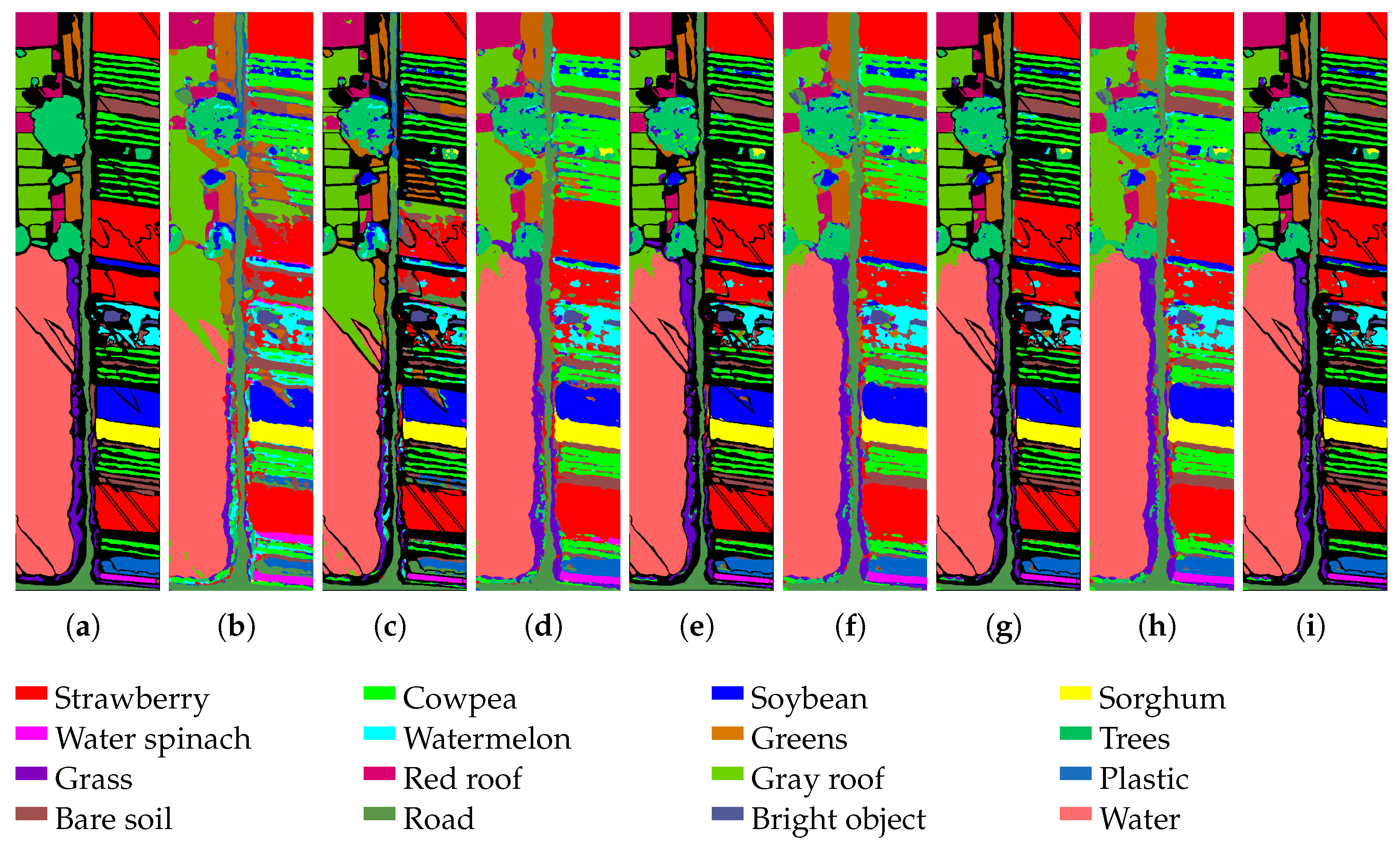
To evaluate the training dynamics and convergence characteristics of DFMamba using the HanChuan dataset as a representative case, prediction results at different training stages were systematically recorded in the validation set. As shown in the visualization sequence in Figure 2, the model progressively improved in classification accuracy and spatial consistency throughout training. At the early stage (epoch 50), predicted maps still had coarse boundaries and some misclassified regions, indicating that the model was primarily learning basic discriminative features. By epoch 100, classification boundaries became clearer, and misclassification areas were reduced. By epoch 150, the model produced accurate classification results with significantly improved spatial consistency. At epoch 200, the model achieved stable and consistent predictions, with clear boundaries and minimal misclassification artifacts, indicating successful convergence. Comparing predictions at different epochs with the ground truth shows that the model effectively learns hierarchical spectral–spatial features for precise pixel-level classification while maintaining spatial consistency among adjacent regions.

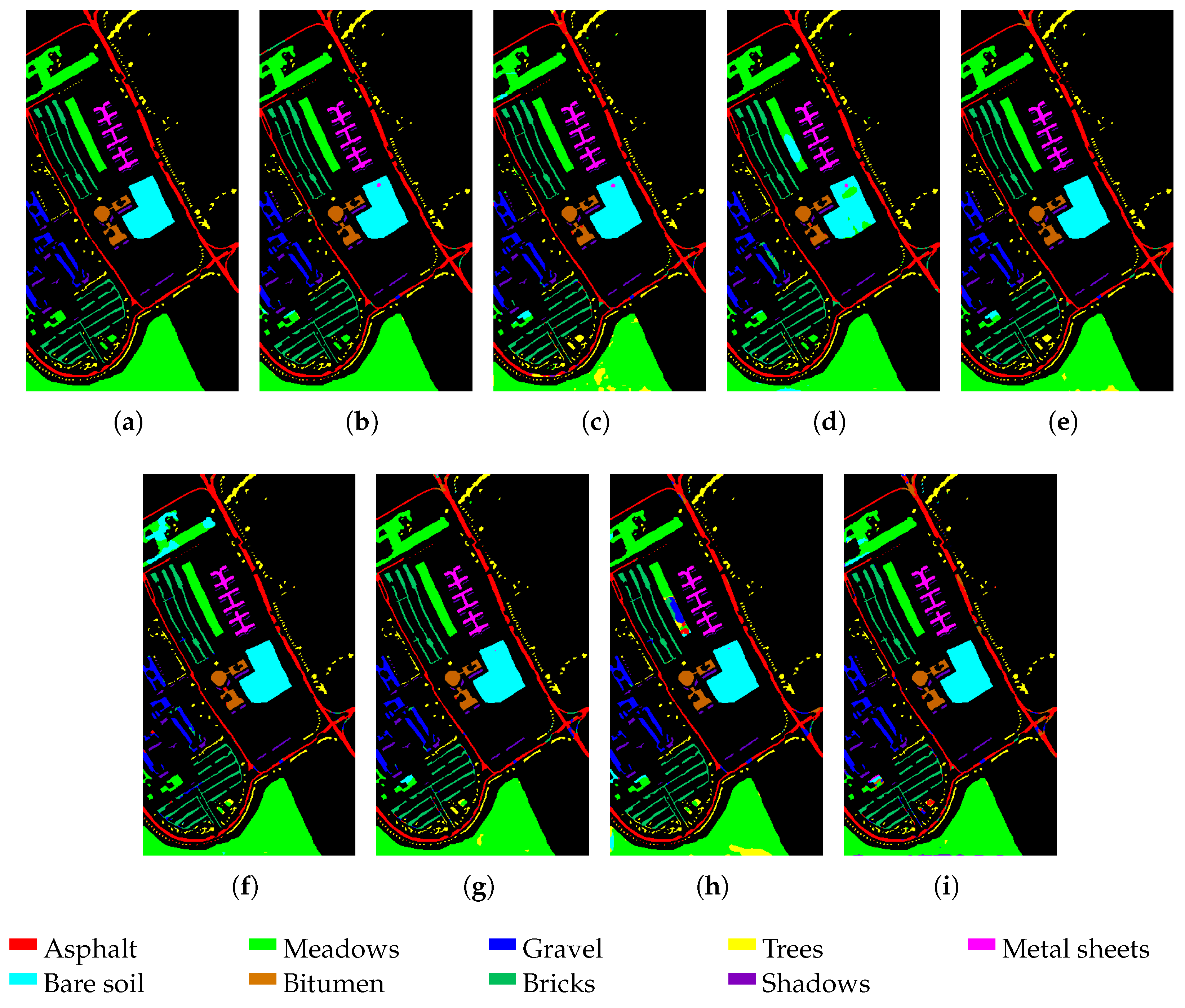
To further illustrate the contributions of key components using the Pavia University dataset as a representative example, Figure 3 presents classification maps generated by different model variants, all displayed after applying the official background mask. From the visual results, it can be seen that the complete improved model (Figure 3b) significantly outperformed the baseline (Figure 3c) in boundary precision and spatial consistency, especially in areas with complex land cover distributions. In contrast, removing the HSAE module (Figure 3d) resulted in blurred boundaries and increased misclassification, validating its importance in feature extraction and channel compression. Variants using only attention fusion (Figure 3e), convolutional fusion (Figure 3f), or dynamic weight fusion (Figure 3g) produced relatively reasonable results but were inferior to the full model in boundary precision and spatial consistency, demonstrating the necessity of component synergy for optimal performance. Variants with gated fusion (Figure 3h) or removal of the improved classification head (Figure 3i) also showed performance degradation, further confirming the effectiveness of the proposed architectural design.

4.8. Inference Scalability with Spectral Sequence Length

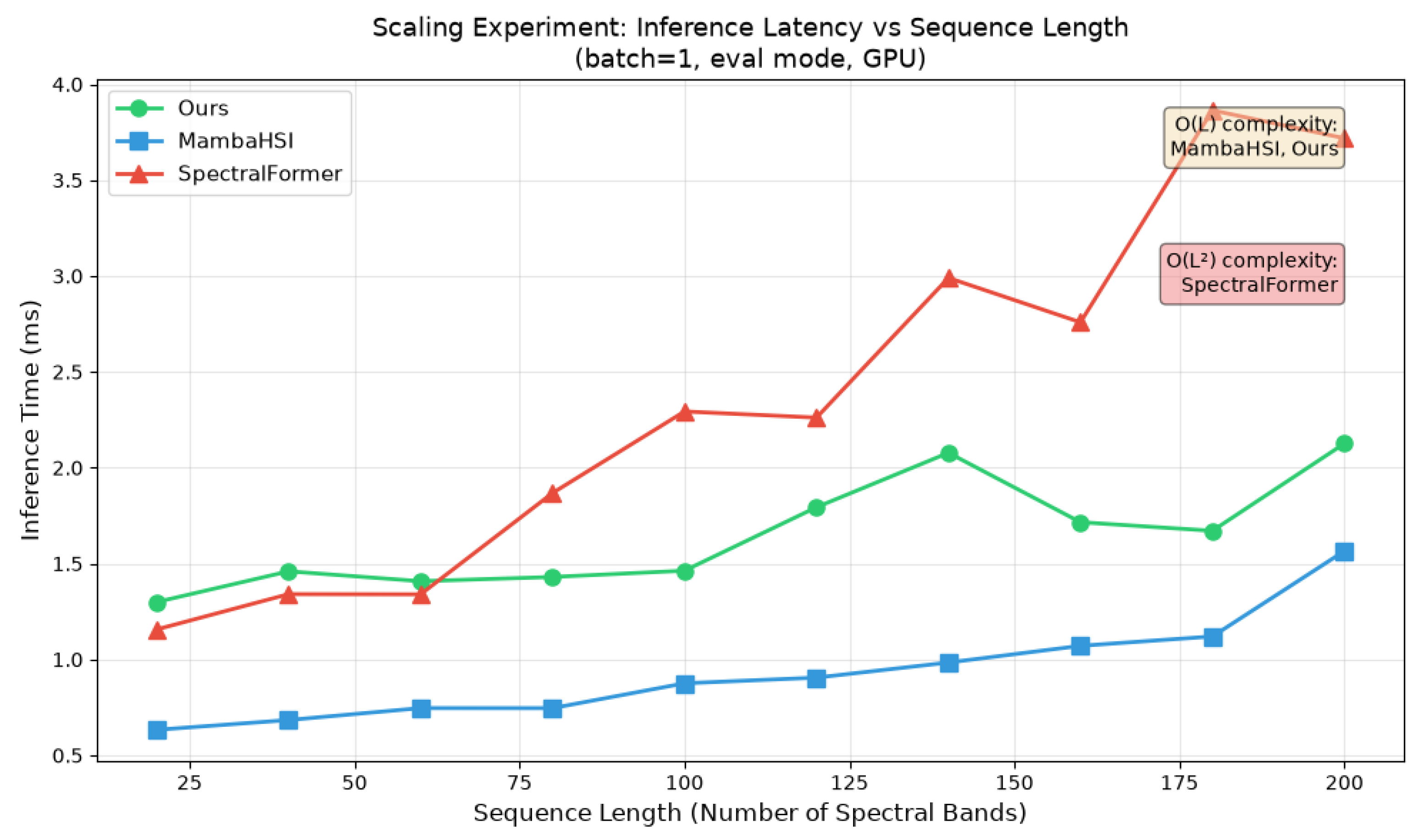
To further evaluate the computational scalability of the proposed method, we investigate how inference latency varies with the spectral sequence length. Let $L=C$ denote the spectral sequence length, where C is the number of input spectral bands. Specifically, C is gradually increased from 20 to 200 while the spatial resolution is fixed at $9\times 9$. Three representative models are compared: the Transformer-based SpectralFormer, the Mamba-based baseline MambaHSI, and the proposed DFMamba. This experiment focuses on the practical scaling behavior of different sequence modeling mechanisms with respect to the spectral dimension.

For a fair comparison, all models are evaluated with a batch size of 1 in evaluation mode, with gradient computation disabled. Before timing, 10 warm-up iterations are performed to reduce initialization and CUDA startup overhead, followed by 50 consecutive forward passes. The median inference latency is reported, and all methods follow the same input configuration and timing protocol. The results are shown in Figure 4. The complexity annotations in the figure indicate the theoretical complexity classes of the corresponding sequence modeling mechanisms rather than fitted empirical growth functions.

As shown in Figure 4, SpectralFormer exhibits the steepest latency-growth trend, increasing from 1.16 ms at $C=20$ to 3.72 ms at $C=200$, corresponding to an increase of approximately $3.21\times$. Although practical GPU execution may introduce deviations from ideal theoretical behavior, the overall trend is consistent with the expected $O\left(C^2\right)$ complexity of self-attention. This result indicates that the computational cost of Transformer-based spectral modeling becomes increasingly significant as the spectral sequence length grows.

For MambaHSI, the inference latency increases from 0.63 ms at $C=20$ to 1.57 ms at $C=200$, corresponding to an increase of approximately $2.49\times$. Its overall latency-growth trend is considerably smoother than that of SpectralFormer and is consistent with the expected $O\left(C\right)$ complexity of state-space sequence modeling. Moreover, the latency ratio between SpectralFormer and MambaHSI increases from approximately $1.83\times$ at $C=20$ to $2.37\times$ at $C=200$, indicating that the computational advantage of linear sequence modeling becomes more evident for longer spectral inputs.

It should be noted that the present experiment compares inference latency under fixed network configurations rather than equivalent classification accuracy. DFMamba introduces additional feature extraction components, including HSAE and the enhanced classification head, to strengthen spatial–spectral representation before and after sequence modeling. These additional convolutional, attention, and multi-branch operations inevitably introduce extra computational overhead, resulting in higher absolute inference latency than MambaHSI. Therefore, the observed latency difference should be interpreted as the computational cost of the enhanced representation capability rather than a change in the linear scalability of the underlying Mamba sequence modeling mechanism.

The inference latency of DFMamba increases from 1.30 ms at $C=20$ to 2.13 ms at $C=200$, corresponding to an endpoint ratio of approximately $1.64\times$. Although its absolute latency is higher than that of MambaHSI, the relative increase across the evaluated sequence-length range is the smallest among the three compared methods. This result indicates that DFMamba is less sensitive to increasing spectral sequence length than SpectralFormer.

The favorable scaling behavior of DFMamba is also consistent with the design of HSAE, which compresses an arbitrary number of input spectral bands into a fixed latent representation of $2N=56$ channels before the subsequent Mamba blocks. Consequently, the feature dimensionality processed by the main Mamba backbone does not increase proportionally with the original number of spectral bands. The additional modules therefore mainly contribute a relatively stable computational overhead, while the dependence of the backbone computation on the spectral sequence length remains consistent with linear-complexity sequence modeling.

Minor non-monotonic variations can be observed at several intermediate sequence lengths. These fluctuations are attributable to normal GPU runtime variability, including CUDA kernel scheduling, cache behavior, memory-access patterns, and hardware-level parallel execution. Their influence is reduced by applying the same warm-up and timing procedure to all methods and reporting the median latency over 50 forward passes. Therefore, the results are interpreted primarily according to the overall scaling trend rather than isolated differences between adjacent sequence lengths.

At $C=200$, DFMamba requires 2.13 ms for one forward pass, whereas SpectralFormer requires 3.72 ms, corresponding to an inference-time ratio of approximately $1.75\times$ in favor of DFMamba. Meanwhile, MambaHSI remains the fastest model in terms of absolute inference latency. These results show that the additional modules introduced in DFMamba incur a moderate computational cost, but do not produce the rapidly increasing latency associated with quadratic self-attention.

Overall, the empirical observations are consistent with the theoretical complexity characteristics of the compared sequence modeling mechanisms. SpectralFormer exhibits substantially faster latency growth because of quadratic self-attention, whereas MambaHSI and DFMamba show overall trends consistent with linear-complexity state-space modeling. Although DFMamba has higher absolute inference latency than MambaHSI owing to its additional feature extraction and classification modules, these components mainly introduce a relatively stable computational overhead. As a result, DFMamba preserves the favorable scalability of Mamba-based sequence modeling and remains substantially less sensitive to increasing spectral sequence length than the Transformer-based baseline.

5. Discussion

5.1. Interpretation of Key Results

The experimental results in Section 4 demonstrate that the proposed DFMamba model consistently achieved competitive classification accuracy and computational efficiency across four benchmark hyperspectral datasets. The HSAE module, which combines adaptive group convolution, depth-wise separable convolution, and spatial attention, was the primary driver of parameter reduction (approximately 70%) and FLOPs reduction (approximately 70–74%) while maintaining or improving accuracy. This is because HSAE effectively compresses highly redundant spectral channels without losing discriminative information, while its spatial-attention operation selectively enhances informative regions. The model without HSAE exhibited consistent OA degradation, including decreases of 0.92 percentage points on UP and 2.70 percentage points on HanChuan, confirming its contribution.

The EnhancedBothMamba module inherits the spatial–spectral dual-branch design from the baseline MambaHSI, where the effectiveness of separately modeling spatial and spectral dependencies has already been demonstrated [26]. Therefore, this study does not repeat the branch-level ablation of SpaMamba and SpeMamba, but instead focuses on evaluating the proposed improvements over the original dual-branch framework. The experimental results demonstrate that the proposed learnable weighted fusion strategy provides more effective feature integration than the compared convolutional fusion and spatial-attention fusion alternatives. This improvement can be attributed to the ability of the learnable fusion weights to optimize the relative contribution of spatial and spectral representations during end-to-end training. Specifically, the fusion coefficients are global model parameters shared across samples, channels, and spatial positions, rather than input-dependent adaptive weights. In addition, the learnable residual factor $\beta$ further adjusts the contribution of shortcut information, improving feature propagation and contributing to the overall robustness of the network.

The improved ClsHead has a substantial impact on complex datasets. For example, on HongHu, which contains 22 classes, removing ClsHead reduced OA by 19.52 percentage points. The dual-branch design of ClsHead, consisting of a local $3\times 3$ convolution for spatial details and a global $1\times 1$ convolution for channel-wise semantics, is essential for separating fine-grained categories such as different crop types. The local branch enhances subtle spatial structures such as field boundaries and texture variations, whereas the global branch refines channel-wise semantic responses by integrating complementary spectral information. Their combination enables more discriminative feature representations for categories with high inter-class similarity. Without this module, the model loses local discriminative cues and relies excessively on global feature maps, leading to severe misclassification, especially for land-cover classes that exhibit similar spectral signatures but differ in fine spatial patterns.

Another important implementation choice is that background or unlabeled pixels are retained during forward propagation but excluded from optimization and quantitative evaluation using the predefined ignore label. This strategy enables dense end-to-end prediction over complete hyperspectral scenes while preventing invalid annotations from affecting parameter optimization. Consequently, the proposed framework simultaneously preserves spatial continuity and ensures a fair evaluation on annotated semantic classes.

5.2. Limitations

Despite its strong performance, DFMamba has several limitations. First, the training setting uses only 30 labeled samples per class, which may not fully exploit the representation capability of state-space models. In extremely low-sample scenarios (e.g., 5–10 samples per class), the model may suffer from overfitting due to insufficient supervision. Second, the model does not incorporate explicit class-rebalancing mechanisms. Although balanced sampling is adopted during training, extremely long-tailed class distributions may still result in biased predictions toward majority classes, and dedicated loss functions or adaptive sampling strategies may be required for highly imbalanced datasets.

Third, although DFMamba achieves linear time complexity, memory consumption still increases with input image size. For instance, on the Houston dataset (349 × 1905 pixels), training required approximately 8 GB of GPU memory. Therefore, patch-based inference or image tiling strategies may still be necessary for processing extremely large-scale hyperspectral scenes.

Fourth, the current model has not been extensively validated under complex real-world conditions. In noisy scenarios, such as images affected by sensor noise or atmospheric interference, classification performance may degrade because the spectral branch relies on fine-grained spectral signatures that can be corrupted by noise. Moreover, cross-domain generalization remains challenging. When hyperspectral images are collected from different sensors, geographical regions, or acquisition conditions, variations in spectral responses and spatial resolutions may introduce domain shifts, limiting the direct transferability of the trained model.

5.3. Future Work

Based on these findings, several promising directions can be explored in future work. Firstly, integrating DFMamba with active learning could reduce the annotation burden by selectively labeling the most informative pixels, which is particularly valuable for hyperspectral applications with limited labeled samples. Secondly, further model compression through knowledge distillation or quantization could improve the deployment capability of DFMamba on resource-constrained platforms such as drones or satellites.

Thirdly, extending the dual-branch architecture to hyperspectral unmixing and change detection is another possible direction, as the spectral branch’s long-range dependency modeling may benefit endmember extraction and temporal spectral analysis. Fourth, to improve cross-scene hyperspectral image classification capability, future research could incorporate domain adaptation techniques, such as adversarial domain adaptation, feature alignment, or meta-learning, to reduce distribution discrepancies between different sensors and geographical regions. In addition, noise-robust training strategies, including spectral denoising modules and noise-aware optimization, could be investigated to enhance model reliability under degraded imaging conditions. Finally, self-supervised pre-training on large-scale unlabeled hyperspectral datasets may provide more robust spatial–spectral representations and further improve the model’s generalization ability in unseen scenarios.

6. Conclusions

In this study, we proposed the DFMamba model for hyperspectral image classification, building on the baseline MambaHSI architecture. The core innovations of the model can be summarized as follows: First, we designed the channel-optimized spatial–spectral module (HSAE), which leverages the synergy of adaptive grouped convolution, depth-wise separable convolution, and spatial attention mechanisms to enhance feature discriminability while reducing parameter count, effectively addressing the high dimensionality and redundancy challenges inherent in hyperspectral data. Secondly, within the inherited spatial–spectral dual-branch Mamba framework, we introduced softmax-normalized learnable global weights and a learnable residual scaling factor $\beta$ to combine the SpaMamba and SpeMamba outputs. Convolutional fusion and spatial-attention fusion were evaluated only as comparison variants. Finally, we constructed an improved classification head, ClsHead, which combines local spatial details and channel-semantic features through a dual-branch aggregation strategy. The model retains the linear-complexity property of Mamba-based sequence modeling, in contrast to the quadratic complexity of standard self-attention.

Experimental results on four standard hyperspectral datasets—Pavia University, Houston, HanChuan, and HongHu—demonstrated that DFMamba achieved competitive performance compared with methods based on traditional machine learning (SVM, RF), graph convolutional networks (DMSGer, GiGCN), convolutional neural networks (FullyContNet, CLOLN), and Transformer architectures (SpectralFormer, GSC-ViT). Moreover, the model retained the favorable linear-complexity characteristics of Mamba-based sequence modeling while achieving efficient computation, supporting the practical potential of the proposed approach. This study demonstrates the applicability of state-space-based Mamba architectures to hyperspectral image classification and provides a promising approach for balancing classification performance and computational efficiency. It also offers useful references for future research in hyperspectral image analysis.

References

1. Ahmad, M.; Distefano, S.; Khan, A.M.; Mazzara, M.; Li, C.; Li, H.; Aryal, J.; Ding, Y.; Vivone, G.; Hong, D. A comprehensive survey for hyperspectral image classification: The evolution from conventional to transformers and mamba models. Neurocomputing 2025, 644, 130428. [Google Scholar] [CrossRef] [Scilit]
2. Wambugu, N.; Chen, Y.; Xiao, Z.; Tan, K.; Wei, M.; Liu, X.; Li, J. Hyperspectral image classification on insufficient-sample and feature learning using deep neural networks: A review. Int. J. Appl. Earth Obs. Geoinf. 2021, 105, 102603. [Google Scholar] [CrossRef] [Scilit]
3. Cheng, M.-F.; Mukundan, A.; Karmakar, R.; Valappil, M.A.E.; Jouhar, J.; Wang, H.-C. Modern trends and recent applications of hyperspectral imaging: A review. Technologies 2025, 13, 170. [Google Scholar] [CrossRef] [Scilit]
4. Pour, A.B.; Zoheir, B.; Pradhan, B.; Hashim, M. Editorial for the special issue: Multispectral and hyperspectral remote sensing data for mineral exploration and environmental monitoring of mined areas. Remote Sens. 2021, 13, 519. [Google Scholar] [CrossRef] [Scilit]
5. Melgani, F.; Bruzzone, L. Classification of hyperspectral remote sensing images with support vector machines. IEEE Trans. Geosci. Remote Sens. 2004, 42, 1778–1790. [Google Scholar] [CrossRef] [Scilit]
6. Pal, M. Random forest classifier for remote sensing classification. Int. J. Remote Sens. 2005, 26, 217–222. [Google Scholar] [CrossRef] [Scilit]
7. Hughes, G. On the mean accuracy of statistical pattern recognizers. IEEE Trans. Inf. Theory 1968, 14, 55–63. [Google Scholar] [CrossRef] [Scilit]
8. Tarabalka, Y.; Benediktsson, J.A.; Chanussot, J. Spectral–spatial classification of hyperspectral imagery based on partitional clustering techniques. IEEE Trans. Geosci. Remote Sens. 2009, 47, 2973–2987. [Google Scholar] [CrossRef] [Scilit]
9. Chen, Y.; Lin, Z.; Zhao, X.; Wang, G.; Gu, Y. Deep learning-based classification of hyperspectral data. IEEE J. Sel. Top. Appl. Earth Obs. Remote Sens. 2014, 7, 2094–2107. [Google Scholar] [CrossRef] [Scilit]
10. Liu, B.; Yu, X.; Zhang, P.; Yu, A.; Fu, Q.; Wei, X. Supervised deep feature extraction for hyperspectral image classification. IEEE Trans. Geosci. Remote Sens. 2018, 56, 1909–1921. [Google Scholar] [CrossRef] [Scilit]
11. Zhong, Z.; Li, J.; Luo, Z.; Chapman, M. Spectral–spatial residual network for hyperspectral image classification: A 3-D deep learning framework. IEEE Trans. Geosci. Remote Sens. 2018, 56, 847–858. [Google Scholar] [CrossRef] [Scilit]
12. Chen, H.; Miao, F.; Chen, Y.; Xiong, Y.; Chen, T. A hyperspectral image classification method using multifeature vectors and optimized KELM. IEEE J. Sel. Top. Appl. Earth Obs. Remote Sens. 2021, 14, 2781–2795. [Google Scholar] [CrossRef] [Scilit]
13. Ahmad, M.; Shabbir, S.; Roy, S.K.; Hong, D.; Wu, X.; Yao, J. Hyperspectral image classification—traditional to deep models: A survey for future prospects. IEEE J. Sel. Top. Appl. Earth Obs. Remote Sens. 2021, 15, 968–999. [Google Scholar] [CrossRef] [Scilit]
14. Roy, S.K.; Krishna, G.; Dubey, S.R.; Chaudhuri, B.B. HybridSN: Exploring 3-D–2-D CNN feature hierarchy for hyperspectral image classification. IEEE Geosci. Remote Sens. Lett. 2020, 17, 277–281. [Google Scholar] [CrossRef] [Scilit]
15. Guidici, D.; Clark, M.L. One-dimensional convolutional neural network land-cover classification of multi-seasonal hyperspectral imagery in the San Francisco Bay Area. Remote Sens. 2017, 9, 629. [Google Scholar] [CrossRef] [Scilit]
16. Mou, L.; Ghamisi, P.; Zhu, X.X. Deep recurrent neural networks for hyperspectral image classification. IEEE Trans. Geosci. Remote Sens. 2017, 55, 3639–3655. [Google Scholar] [CrossRef] [Scilit]
17. Zhao, W.; Du, S. Spectral–spatial feature extraction for hyperspectral image classification: A dimension reduction and deep learning approach. IEEE Trans. Geosci. Remote Sens. 2016, 54, 4544–4554. [Google Scholar] [CrossRef] [Scilit]
18. Mei, S.; Li, X.; Liu, X.; Cai, H.; Du, Q. Hyperspectral image classification using attention-based bidirectional long short-term memory network. IEEE Trans. Geosci. Remote Sens. 2021, 60, 5509612. [Google Scholar] [CrossRef] [Scilit]
19. Vaswani, A.; Shazeer, N.; Parmar, N.; Uszkoreit, J.; Jones, L.; Gomez, A.N.; Kaiser, Ł.; Polosukhin, I. Attention Is All You Need. In Advances in Neural Information Processing Systems; Curran Associates, Inc.: Red Hook, NY, USA, 2017; Volume 30, pp. 5998–6008. [Google Scholar]
20. Dosovitskiy, A.; Beyer, L.; Kolesnikov, A.; Weissenborn, D.; Zhai, X.; Unterthiner, T.; Dehghani, M.; Minderer, M.; Heigold, G.; Gelly, S.; et al. An Image Is Worth 16×16 Words: Transformers for Image Recognition at Scale. In Proceedings of the International Conference on Learning Representations (ICLR), Virtual Event, Austria, 3–7 May 2021. [Google Scholar]
21. Liu, Z.; Lin, Y.; Cao, Y.; Hu, H.; Wei, Y.; Zhang, Z. Swin Transformer: Hierarchical Vision Transformer Using Shifted Windows. In Proceedings of the IEEE/CVF International Conference on Computer Vision, Montreal, QC, Canada, 10–17 October 2021; pp. 10012–10022. [Google Scholar] [CrossRef] [Scilit]
22. Hong, D.; Han, Z.; Yao, J.; Gao, L.; Zhang, B.; Plaza, A.; Chanussot, J. SpectralFormer: Rethinking Hyperspectral Image Classification with Transformers. IEEE Trans. Geosci. Remote Sens. 2022, 60, 5518615. [Google Scholar] [CrossRef] [Scilit]
23. Sun, L.; Zhao, G.; Zheng, Y.; Wu, Z. Spectral–spatial feature tokenization transformer for hyperspectral image classification. IEEE Trans. Geosci. Remote Sens. 2022, 60, 5522214. [Google Scholar] [CrossRef] [Scilit]
24. Yang, X.; Cao, W.; Lu, Y.; Zhou, Y. Hyperspectral image transformer classification networks. IEEE Trans. Geosci. Remote Sens. 2022, 60, 5528715. [Google Scholar] [CrossRef] [Scilit]
25. He, X.; Chen, Y.; Lin, Z. Spatial–spectral transformer for hyperspectral image classification. Remote Sens. 2021, 13, 498. [Google Scholar] [CrossRef] [Scilit]
26. Li, Y.; Luo, Y.; Zhang, L.; Wang, Z.; Du, B. MambaHSI: Spatial-Spectral Mamba for Hyperspectral Image Classification. IEEE Trans. Geosci. Remote Sens. 2024, 62, 5524216. [Google Scholar] [CrossRef] [Scilit]
27. Gu, A.; Dao, T. Mamba: Linear-time sequence modeling with selective state spaces. In Proceedings of the First Conference on Language Modeling, Philadelphia, PA, USA, 7–9 October 2024. [Google Scholar]
28. Tarabalka, Y.; Tilton, J.C.; Benediktsson, J.A.; Chanussot, J. Spectral–spatial classification of hyperspectral images using partitional clustering techniques. IEEE J. Sel. Top. Appl. Earth Obs. Remote Sens. 2011, 5, 262–272. [Google Scholar]
29. Shi, X.; Liu, L.; Bao, X.; Pan, B.; Hussain, S. Dynamic gated fusion network with hierarchical multi-scale attention for hyperspectral image classification. Sci. Rep. 2025, 15, 44289. [Google Scholar] [CrossRef] [Scilit] [PubMed]
30. Yao, J.; Hong, D.; Li, C.; Chanussot, J. SpectralMamba: Efficient mamba for hyperspectral image classification. arXiv 2024, arXiv:2404.08489. [Google Scholar]
31. He, Y.; Tu, B.; Liu, B.; Li, J.; Plaza, A. 3DSS-Mamba: 3D-Spectral-Spatial Mamba for Hyperspectral Image Classification. IEEE Trans. Geosci. Remote Sens. 2024, 62, 5534216. [Google Scholar] [CrossRef] [Scilit]
32. Wang, C.; Huang, J.; Lv, M.; Du, H.; Wu, Y.; Qin, R. A local enhanced mamba network for hyperspectral image classification. Int. J. Appl. Earth Obs. Geoinf. 2024, 133, 104092. [Google Scholar] [CrossRef] [Scilit]
33. Wang, Y.; Cao, G.; Shi, B.; Zhang, Y. CF-Mamba: A Dual-Path Collaborative Method for Hyperspectral Image Classification. Remote Sens. 2026, 18, 1063. [Google Scholar] [CrossRef] [Scilit]
34. Author, N. BiMambaHSI: Bidirectional Spectral–Spatial State Space Model for Hyperspectral Image Classification. Remote Sens. 2025, 17, 3676. [Google Scholar] [CrossRef] [Scilit]
35. Fauvel, M.; Tarabalka, Y.; Benediktsson, J.A.; Chanussot, J.; Tilton, J.C. Advances in Spectral–Spatial Classification of Hyperspectral Images. Proc. IEEE 2013, 101, 652–675. [Google Scholar] [CrossRef] [Scilit]
36. Benediktsson, J.A.; Palmason, J.A.; Sveinsson, J.R. Classification of hyperspectral data from urban areas based on extended morphological profiles. IEEE Trans. Geosci. Remote Sens. 2005, 43, 480–491. [Google Scholar] [CrossRef] [Scilit]
37. Su, H.; Hu, Y.; Lu, H.; Sun, W.; Du, Q. Diversity-driven multikernel collaborative representation ensemble for hyperspectral image classification. IEEE J. Sel. Top. Appl. Earth Obs. Remote Sens. 2022, 15, 2861–2876. [Google Scholar] [CrossRef] [Scilit]
38. Makantasis, K.; Karantzalos, K.; Doulamis, A.; Doulamis, N. Deep supervised learning for hyperspectral data classification through convolutional neural networks. In Proceedings of the IEEE International Geoscience and Remote Sensing Symposium (IGARSS), Milan, Italy, 26–31 July 2015; pp. 4959–4962. [Google Scholar] [CrossRef] [Scilit]
39. Alhassan, A.M.; Alzahrani, S.; Aldawsari, A.; Alshahrani, S. SF-ICNN: Spectral–Fractal Iterative Convolutional Neural Network for Classification of Hyperspectral Images. Appl. Sci. 2022, 14, 7361. [Google Scholar] [CrossRef] [Scilit]
40. Paoletti, M.E.; Moreno-Álvarez, S.; Xue, Y.; Haut, J.M.; Plaza, A. AAtt-CNN: Automatic attention-based convolutional neural networks for hyperspectral image classification. IEEE Trans. Geosci. Remote Sens. 2023, 61, 5511118. [Google Scholar] [CrossRef] [Scilit]
41. Zhai, H.; Zhao, J. Two-stream spectral-spatial convolutional capsule network for hyperspectral image classification. Int. J. Appl. Earth Obs. Geoinf. 2024, 127, 103614. [Google Scholar] [CrossRef] [Scilit]
42. Zhao, Z.; Xu, X.; Li, S.; Plaza, A. Hyperspectral image classification using groupwise separable convolutional vision transformer network. IEEE Trans. Geosci. Remote Sens. 2024, 62, 5511817. [Google Scholar] [CrossRef] [Scilit]
43. Liu, P.; Zhang, H.; Eom, K.B. Active deep learning for classification of hyperspectral images. IEEE J. Sel. Top. Appl. Earth Obs. Remote Sens. 2016, 10, 712–724. [Google Scholar] [CrossRef] [Scilit]
44. Qin, A.; Shang, Z.; Tian, J.; Wang, Y.; Zhang, T.; Tang, Y.Y. Spectral–spatial graph convolutional networks for semisupervised hyperspectral image classification. IEEE Geosci. Remote Sens. Lett. 2019, 16, 241–245. [Google Scholar] [CrossRef] [Scilit]
45. Zhang, H.; Zou, J.; Zhang, L. EMS-GCN: An end-to-end mixhop superpixel-based graph convolutional network for hyperspectral image classification. IEEE Trans. Geosci. Remote Sens. 2022, 60, 5526116. [Google Scholar] [CrossRef] [Scilit]
46. Jia, S.; Jiang, S.; Zhang, S.; Xu, M.; Jia, X. Graph-in-graph convolutional network for hyperspectral image classification. IEEE Trans. Neural Netw. Learn. Syst. 2024, 35, 1157–1171. [Google Scholar] [CrossRef] [Scilit] [PubMed]
47. Yang, Y.; Zhong, P.; Zhang, L.; Li, Z.; Zhang, L. Semi-Supervised Multiscale Dynamic Graph Convolution Network for Hyperspectral Image Classification. IEEE Trans. Neural Netw. Learn. Syst. 2024, 35, 1025–1038. [Google Scholar] [CrossRef] [Scilit] [PubMed]
48. Jiang, Y.; Zhang, Z.; Zhang, C.; Zhou, H.; Ma, Q.; Zhong, C. S2WaveNet: A novel spectral–spatial wave network for hyperspectral image classification. Int. J. Appl. Earth Obs. Geoinf. 2024, 128, 103754. [Google Scholar] [CrossRef] [Scilit]
49. Zou, J.; He, W.; Wang, H.; Zhang, H. SAM-CTMapper: Utilizing segment anything model and scale-aware mixed CNN-Transformer facilitates coastal wetland hyperspectral image classification. Int. J. Appl. Earth Obs. Geoinf. 2025, 139, 104469. [Google Scholar] [CrossRef] [Scilit]
50. Xue, Z.; Xu, Q.; Zhang, M. Local transformer with spatial partition restore for hyperspectral image classification. IEEE J. Sel. Top. Appl. Earth Obs. Remote Sens. 2022, 15, 4307–4325. [Google Scholar] [CrossRef] [Scilit]
51. Kalman, R.E. A new approach to linear filtering and prediction problems. J. Basic Eng. 1960, 82, 35–45. [Google Scholar] [CrossRef] [Scilit]
52. Tu, B.; Zhou, T.; Liu, B.; He, Y.; Li, J.; Plaza, A. Multi-Scale Autoencoder Suppression Strategy for Hyperspectral Image Anomaly Detection. IEEE Trans. Image Process. 2025, 34, 5115–5130. [Google Scholar] [CrossRef] [Scilit] [PubMed]
53. Lin, Y.; Zhu, Z.; Guo, Y.; Ou, Z.; Yao, S.; Song, M. Exploring Inter-Domain Wasserstein Metric for Adaptive Object Detection. In IEEE Transactions on Multimedia; IEEE: Piscataway, NJ, USA, 2026; pp. 1–11. [Google Scholar] [CrossRef] [Scilit]
54. Wu, X.; Wang, C.; Song, C.; Fu, Q.; Liu, J.; Liu, J.; Wang, Q.; Shi, H. Polarization Super-Resolution Remote Sensing Imaging Based on Compressed Sensing and Deep Learning. IEEE Trans. Geosci. Remote Sens. 2026, 64, 5613426. [Google Scholar] [CrossRef] [Scilit]
55. Yang, Z.; Xia, J.; Li, S.; Zheng, L.; Zhang, S.; Liu, L.; Fu, Y.; Liu, Y. Band-Kernel Stochastic Learning for Unsupervised Blind Hyperspectral Image Super-Resolution. IEEE Trans. Pattern Anal. Mach. Intell. 2026, 48, 9895–9913. [Google Scholar] [CrossRef] [Scilit] [PubMed]
56. Gu, A.; Goel, K.; Ré, C. Efficiently Modeling Long Sequences with Structured State Spaces. In Proceedings of the International Conference on Learning Representations (ICLR), Virtual, 25–29 April 2022. [Google Scholar]
57. Smith, J.T.H.; Warrington, A.; Linderman, S.W. Simplified State Space Layers for Sequence Modeling. In Proceedings of the International Conference on Learning Representations (ICLR), Kigali, Rwanda, 1–5 May 2023. [Google Scholar]
58. Fu, D.Y.; Dao, T.; Saab, K.K.; Thomas, A.W.; Rudra, A.; Ré, C. Hungry Hungry Hippos: Towards Language Modeling with State Space Models. In Proceedings of the International Conference on Learning Representations (ICLR), Kigali, Rwanda, 1–5 May 2023. [Google Scholar]
59. Mehta, H.; Gupta, A.; Cutkosky, A.; Neyshabur, B. Long Range Language Modeling via Gated State Spaces. In Proceedings of the International Conference on Learning Representations (ICLR), Kigali, Rwanda, 1–5 May 2023. [Google Scholar]
60. Nguyen, E.; Goel, K.; Gu, A.; Downs, G.W.; Shah, P.; Dao, T.; Baccus, S.A.; Ré, C. S4ND: Modeling images and videos as multidimensional signals using state spaces. Proc. Adv. Neural Inf. Process. Syst. 2022, 35, 2846–2861. [Google Scholar] [CrossRef] [Scilit]
61. Islam, M.M.; Hasan, M.; Athrey, K.S.; Braskich, T.; Bertasius, G. Efficient movie scene detection using state-space transformers. In Proceedings of the IEEE/CVF Conference on Computer Vision and Pattern Recognition (CVPR), Vancouver, BC, Canada, 17–24 June 2023; pp. 18749–18758. [Google Scholar] [CrossRef] [Scilit]
62. Wang, J.; Zhu, W.; Wang, P.; Yu, X.; Liu, L.; Omar, M.; Hamid, R. Selective structured state-spaces for long-form video understanding. In Proceedings of the IEEE/CVF Conference on Computer Vision and Pattern Recognition (CVPR), Vancouver, BC, Canada, 18–22 June 2023; pp. 6387–6397. [Google Scholar] [CrossRef] [Scilit]
63. Ruan, J.; Li, J.; Xiang, S. VM-UNet: Vision Mamba UNet for Medical Image Segmentation. arXiv 2024, arXiv:2402.02491. [Google Scholar]
64. Wang, D.; Du, B.; Zhang, L. Fully contextual network for hyperspectral scene parsing. IEEE Trans. Geosci. Remote Sens. 2022, 60, 5501316. [Google Scholar] [CrossRef] [Scilit]
65. Li, C.; Rasti, B.; Tang, X.; Duan, P.; Li, J.; Peng, Y. Channel-layer-oriented lightweight spectral–spatial network for hyperspectral image classification. IEEE Trans. Geosci. Remote Sens. 2024, 62, 5504214. [Google Scholar] [CrossRef] [Scilit]
Figure 1. Overall architecture of DFMamba, including the HSAE module, three layers of EnhancedBothMamba modules, and the ClsHead module.
Remotesensing 18 02526 g001
Figure 2. Visualization of prediction results on the Hanchuan dataset at different epochs: (a) ground truth (masked version), (b) predictions at the 50th epoch, (c) predictions at the 50th epoch (masked version), (d) predictions at the 100th epoch, (e) predictions at the 100th epoch (masked version), (f) predictions at the 150th epoch, (g) predictions at the 150th epoch (masked version), (h) predictions at the 200th epoch, and (i) predictions at the 200th epoch (masked version).
Remotesensing 18 02526 g002
Figure 3. Classification maps (background masked in black) for the Pavia University dataset: (a) ground truth, (b) predictions of the complete improved model, (c) predictions of the baseline model, (d) predictions without the HSAE module, (e) predictions with the attention fusion mechanism and β , (f) predictions with the convolutional fusion mechanism and β , (g) predictions with the dynamic weight fusion mechanism and without β , (h) predictions with the gated fusion mechanism, and (i) predictions without the improved classification head.
Remotesensing 18 02526 g003
Figure 4. Inference latency under increasing spectral sequence lengths. The number of spectral bands is varied from 20 to 200 while the spatial resolution is fixed at 9 × 9 . SpectralFormer exhibits a substantially steeper latency-growth trend, whereas the overall trends of MambaHSI and DFMamba are consistent with the expected linear-complexity behavior of Mamba-based sequence modeling.
Remotesensing 18 02526 g004