Influence of Lens Distortion Correction and Image Resampling on Vehicle Detection in UAV Imagery

Highlights

What are the main findings?

• Modified original images achieved the highest detection performance among the evaluated preprocessing conditions, with final AP and AR values of 0.662 and 0.737, respectively.
• Lens-corrected images generated using bilinear and nearest-neighbor interpolation showed lower detection performance than the original and modified original images.

What are the implications of the main findings?

• Lens distortion correction does not necessarily improve deep learning-based vehicle detection in wide-angle UAV imagery.
• UAV image preprocessing should be selected based on downstream detection performance rather than geometric correction alone.

Abstract

Unmanned Aerial Vehicles (UAVs) provide high-resolution imagery for detailed object detection, but wide-angle lenses can introduce radial and tangential distortions that affect object geometry and detection performance. This study evaluated the effects of lens distortion correction and image preprocessing on UAV-based vehicle detection. Four preprocessing conditions were compared: Original Image (OI), Modified Original Image (MOI), Bilinear, and Nearest, where Bilinear and Nearest denote lens-corrected images generated using bilinear and nearest-neighbor interpolation. Two convolutional neural network (CNN)-based two-stage object detectors, Faster R-CNN and Cascade R-CNN, were combined with three backbone networks, ResNet-50 (R50), ResNet-101 (R101), and ResNeXt-101 (X101). In total, 24 experimental conditions were evaluated using COCO-based AP and AR metrics. At the final checkpoint, Cascade R-CNN achieved AP and AR values of 0.644 and 0.724, respectively, compared with 0.619 and 0.706 for Faster R-CNN. Among the backbones, R50 showed the most favorable balance between detection accuracy and training time. For image preprocessing, MOI achieved the highest final AP and AR values of 0.662 and 0.737, followed by OI, Bilinear, and Nearest. Bilinear and Nearest retained only 0.944 and 0.938 of the final AP of OI, respectively. These findings indicate that lens distortion correction does not necessarily improve UAV-based vehicle detection and that preprocessing strategies should be selected by considering both geometric correction and downstream detection performance.

1. Introduction

Unmanned Aerial Vehicles (UAVs) have become a powerful tool in remote sensing applications owing to their flexibility, high spatial resolution, and relatively low operational cost compared to traditional aerial or satellite platforms [1]. UAVs are increasingly used for urban monitoring, traffic management, environmental observation, and security surveillance, where detailed information at the object level is essential [2,3]. The ability of UAVs to acquire centimeter-level imagery enables the detection of small objects such as vehicles, which are commonly evaluated in UAV and aerial object detection benchmarks [4,5,6]. This capability is particularly useful in dense and complex environments. However, UAV imagery also introduces challenges, including variable illumination, occlusions, and geometric distortion. These issues are compounded by lens distortions caused by wide-angle lenses.

An often underestimated factor in UAV-based object detection is lens distortion. Commercial UAVs typically employ wide-angle lenses to maximize coverage. However, these lenses introduce radial and tangential distortions that can warp image geometry and object shape, especially near image boundaries [7]. Such distortions can reduce detection accuracy by altering vehicle shapes and scales [8]. Lens distortion correction based on radial and tangential distortion models can mitigate geometric distortion; however, the accompanying remapping and interpolation processes can modify local texture, reduce edge sharpness, and introduce resampling artifacts [9,10,11]. Previous studies have suggested that distortion and rectification in wide-angle or fisheye imagery can affect downstream detection performance by changing object geometry, boundary representation, and local image information [12,13]. Therefore, it is necessary to carefully evaluate the trade-off between geometric distortion correction and information preservation when preparing UAV images for deep learning-based object detection.

This study investigates whether lens distortion correction is beneficial for deep learning–based vehicle detection in nadir UAV imagery acquired with wide-angle lenses in urban and parking lot environments. To evaluate this effect, four image preprocessing conditions were compared: Original Image (OI), Modified Original Image (MOI), Bilinear, and Nearest. OI consisted of original images without lens distortion correction, whereas MOI was generated by cropping the original images to match the effective field of view of the lens-corrected images. Bilinear and Nearest represented lens-corrected images generated using bilinear and nearest-neighbor interpolation, respectively. This design allowed the effects of peripheral cropping and interpolation-based remapping to be examined separately from the use of lens-corrected images. These preprocessing conditions were evaluated using two representative two-stage object detectors, Faster R-CNN and Cascade R-CNN, combined with three backbone networks, ResNet-50 (R50), ResNet-101 (R101), and ResNeXt-101 (X101), to examine the trade-off between detection accuracy and computational efficiency [14,15]. In total, 24 experimental conditions were tested to analyze the effects of image preprocessing, detector architecture, and backbone architecture on detection accuracy, recall, and training time. In addition, sharpness-based image quality metrics and the Metashape image quality score were used to interpret blur and image degradation associated with lens correction and interpolation [16,17,18,19].

The main contributions of this study are as follows: (1) a UAV-based vehicle dataset was constructed to evaluate the role of lens distortion correction in object detection; (2) the effects of image preprocessing were systematically evaluated under controlled detector–backbone settings across 24 experimental conditions; and (3) sharpness-based image quality metrics were integrated to interpret performance differences among uncorrected, cropped, and lens-corrected images.

2. Materials and Methods

2.1. Research Area and Data Collection

This study was conducted at the Daeyeon Campus of Pukyong National University in Busan, South Korea. The site was selected because of its high accessibility and the presence of more than 500 parked vehicles, which provided suitable conditions for UAV-based vehicle detection experiments. The study area covered approximately 100,000 m² and included several parking lots with different vehicle densities. These spatial variations provided diverse vehicle distributions for constructing the UAV image dataset. Image acquisition was conducted over two days, on 13 and 16 January 2025, under clear weather conditions to ensure consistent image quality and sufficient data diversity.

UAV image acquisition was performed using a DJI Mavic 3 Enterprise (M3E, Manufacturer: DJI; manufactured in Shenzhen, China) equipped with wide-angle and telephoto cameras. In this study, only the wide-angle camera was used for lens distortion correction and deep learning experiments. The wide-angle camera has a 4/3 CMOS sensor with an image resolution of 5280 × 3956 pixels. The lens supports a variable aperture range of f/2.8–f/11 and an ISO range of 100–6400. Its field of view (FOV) is 84° diagonally, 70.8° horizontally, and 56° vertically [20]. The M3E was selected because it uses both a mechanical shutter and an electronic shutter, which can reduce rolling shutter distortion compared with UAV models that rely only on electronic rolling shutters [21,22].

This study used Shutter Priority Mode to minimize image blur caused by UAV flight speed. Therefore, the shutter speed was fixed at 1/400 s, ISO values were maintained between 100 and 110, and the aperture values ranged from f/4.5 to f/8. Flights were performed using a double-grid flight pattern, with both forward overlap and side overlap set to 60%. Flight altitudes ranged from 120 m to 150 m at 10 m intervals. The total number of images acquired at 120, 130, 140, and 150 m was 26, 23, 23, and 21, respectively.

The ground sample distance (GSD) was calculated using the formula (H/37.54) cm/pixel, where H is the flight altitude in meters. Accordingly, the GSD ranged from approximately 3.2 to 4.0 cm/pixel at altitudes between 120 m and 150 m. The number of acquired images and the corresponding GSD, F-stop, and ISO values for each date and altitude are summarized in

Table 1. Number of acquired UAV images and camera settings by date and flight altitude.

Date	Flight Altitude	120 m	130 m	140 m	150 m
	GSD (cm)	3.2	3.5	3.7	4.0
13 January 2025	Images	18	16	16	14
	F-stop	5	4.9	4.8	4.8
	ISO	104	100.8	102.7	101.7
16 January 2025	Images	8	7	7	7
	F-stop	5.7	5.7	5.6	5.9
	ISO	101.3	101.3	103.3	101.4

.

2.2. Dataset Construction

The dataset was divided into training and validation sets. The training set consisted of 64 images acquired on 13 January 2025, whereas the validation set consisted of 29 images acquired on 16 January 2025. The train–validation split was performed at the original UAV image level before tiling, and tiling was then applied independently to each split. Overall, the dataset split corresponded to an approximate ratio of 7:3. The number of vehicle instances in each split for the OI, MOI, and LCI datasets is summarized in

Table 2. Number of vehicles before and after image tiling by dataset type and split. (Unit: ea.).

Type	Tiling	Train	Validation	Total
OI	Before	9271	3726	12,997
	After	16,931	6779	23,710
MOI	Before	8603	3396	11,999
	After	16,021	6329	22,350
LCI	Before	8621	3387	12,008
	After	15,897	6158	22,055

.

Ground truth annotations were generated in the PASCAL VOC XML format for training and evaluating the Faster R-CNN and Cascade R-CNN models [23]. LabelImg, an open-source annotation tool, was used for manual labeling [24]. LabelImg supports both single and multiple object annotations per image and is widely adopted in object detection research due to its efficiency in handling multiple objects.

The dataset was categorized into three image groups according to the preprocessing procedure: Original Image (OI), Modified Original Image (MOI), and Lens Corrected Image (LCI). For the detection experiments, the LCI group was further divided into two preprocessing conditions, Bilinear and Nearest, according to the interpolation method. The OI dataset consisted of the full original images without lens distortion correction and therefore retained all peripheral image regions and objects. Lens distortion correction changes the image-coordinate geometry and valid image extent, which inevitably removes or excludes some peripheral pixels and objects. To control for this change in valid extent, the MOI dataset was generated by cropping OI according to the valid image boundary of the lens-corrected images. The cropping extent was determined directly from the valid corrected-image region rather than by arbitrary manual selection. Consequently, MOI, Bilinear, and Nearest represented the same valid scene extent and the same peripheral-object inclusion conditions. MOI preserved the original pixel values within this common extent, whereas Bilinear and Nearest underwent lens-distortion remapping and interpolation. The LCI dataset consisted of images corrected for lens distortion. In this study, the LCI dataset was further generated using two interpolation methods, bilinear interpolation and nearest-neighbor interpolation, to evaluate the effect of interpolation during lens correction.

In the MOI dataset, objects located in the removed peripheral regions were excluded from labeling. In the LCI dataset, lens distortion was reduced, but some objects near the image boundaries were partially cropped or removed during the correction process. Lens correction was performed using interior orientation parameters derived from the Agisoft Metashape (Professional Edition Version 2.3 used) frame camera model, and the image remapping procedure was implemented in Python using OpenCV-based remapping [25,26]. Because bilinear and nearest-neighbor interpolation were applied using the same correction geometry, the two LCI variants shared the same object annotations and object counts. This dataset configuration allowed the effects of distortion removal, image cropping, and interpolation-based lens correction on detection performance to be evaluated. 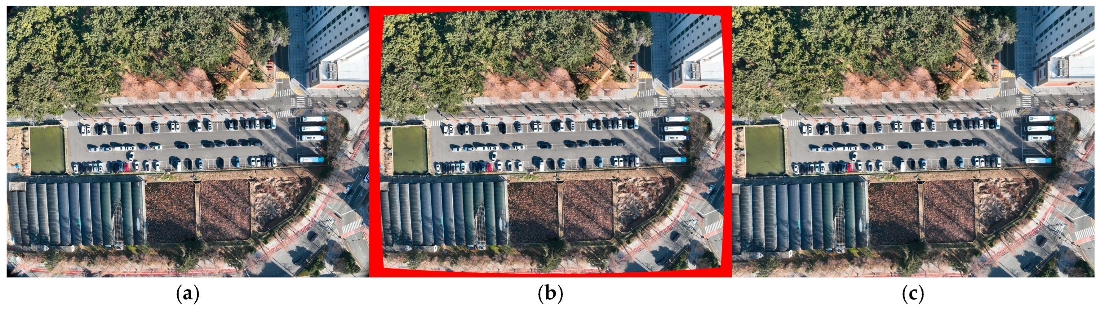Examples of the three image types are illustrated in Figure 1.

For the Faster R-CNN and Cascade R-CNN experiments, tiling was applied to adapt the large UAV images to the network input size. This tiling strategy increased the relative scale of vehicle objects within each network input and helped improve detection performance [27]. Each 5280 × 3956 image was divided into 1024 × 1024 pixel tiles with an overlap of 256 pixels, resulting in 35 tiles per image. The stride size was set to 768 pixels, corresponding to the tile size minus the overlap. Additional tiles were generated at the image boundaries to ensure full spatial coverage. After tiling, objects smaller than 12 pixels in width or height were excluded, and approximately 30% of background-only tiles were randomly retained.

The changes in object counts before and after tiling are summarized in Table 2. Before tiling, the OI, MOI, and LCI datasets contained 12,997, 11,999, and 12,008 objects, respectively. Compared with OI, the MOI and LCI datasets contained fewer objects because of distortion-related boundary exclusions. After tiling, the object counts increased to 23,710, 22,350, and 22,055 for the OI, MOI, and LCI datasets, respectively. The increase in object counts after tiling was mainly caused by duplicated object appearances in overlapping tile regions. The training and validation splits showed similar proportions across image types, with ratios of approximately 71–72% and 28–29%, respectively.

2.3. Lens Distortion Correction

This study used the Agisoft Metashape frame camera model to correct radial and tangential lens distortions [25]. The original UAV images acquired with the DJI Mavic 3 Enterprise RTK were aligned in Agisoft Metashape using the RTK-derived camera positions as positional constraints. During image alignment and bundle adjustment, the camera exterior orientation parameters and interior orientation parameters (IOPs) were estimated and refined. The calibration results and parameter correlations were examined using the Camera Calibration and Distortion Plot tools, followed by camera optimization for the focal length $\mathrm{f}$, principal point offsets ${\mathrm{C}}_{\mathrm{x}}$ and ${\mathrm{C}}_{\mathrm{y}}$, radial distortion coefficients ${\mathrm{K}}_1$–${\mathrm{K}}_4$, tangential distortion coefficients ${\mathrm{P}}_1$ and ${\mathrm{P}}_2$, and affinity/skew coefficients ${\mathrm{B}}_1$ and ${\mathrm{B}}_2$.

The calibrated IOPs were then used for lens distortion correction and image remapping. The full Metashape frame camera model supports $f$, $C_x$, $C_y$, $K_1$–$K_4$, $P_1$, $P_2$, $B_1$, and $B_2$, as expressed in Equations (1)–(9). In the actual OpenCV-based image remapping, only $f$, $C_x$, $C_y$, $K_1$–$K_3$, $P_1$, and $P_2$ were applied, whereas $K_4$, $B_1$, and $B_2$ were not included in the implemented remapping model.

In this model, (X, Y) represents the input image coordinates in the camera coordinate system, and (u, v) denotes the projected pixel coordinates in the image. The image width and height are represented by w and h, respectively. The normalized image coordinates x and y are defined in Equation (1), and the radial distance r from the principal point is defined in Equation (2):

$$x={\displaystyle \frac{X}{f}},y={\displaystyle \frac{Y}{f}}$$

(1)

$$r=\sqrt{\left(x^2+y^2\right)}$$

(2)

Radial distortion occurs when light rays bend as they pass through the lens, causing straight lines to curve. In the Metashape frame camera model, the radial distortion component is expressed using Equations (3) and (4):

$$x_{radial}=x\times (1+K_1\times r^2+K_2\times r^4+K_3\times r^6+K_4\times r^8)$$

(3)

$$y_{radial}=y\times (1+K_1\times r^2+K_2\times r^4+K_3\times r^6+K_4\times r^8)$$

(4)

Tangential distortion arises when the lens and the image plane are not perfectly parallel, resulting in a shift in image points. In the Metashape frame camera model, the tangential distortion component is expressed using Equations (5) and (6):

$$x_{tangential}=(P_1\times (r^2+2\times x^2)+2{\times P}_2\times x\times y)$$

(5)

$$y_{tangential}=(P_2\times (r^2+2\times y^2)+2{\times P}_1\times \mathrm{x}\times \mathrm{y})$$

(6)

The final corrected coordinates x′, y′ are obtained by summing the radial and tangential distortion components, as shown in Equation (7).

$$x^{\prime }=x_{radial}+x_{tangential},y^{\prime }=y_{radial}+y_{tangential}$$

(7)

Finally, the image (pixel) coordinates u, v were obtained by incorporating the focal length, principal point offsets, and skew coefficients, as expressed in Equations (8) and (9):

$$u=w\times 0.5+c_x+x^{\prime }\times f+x^{\prime }\times B_1+y^{\prime }\times B_2$$

(8)

$$v=h\times 0.5+c_y+y^{\prime }\times f$$

(9)

Because lens distortion correction involves geometric remapping, pixel values at the corrected coordinates must be resampled. In this study, two interpolation methods were applied during the remapping process: bilinear interpolation and nearest-neighbor interpolation. Bilinear interpolation estimates new pixel values using a weighted average of neighboring pixels, which can produce smoother images but may reduce edge sharpness. Nearest-neighbor interpolation assigns the value of the closest input pixel, preserving original pixel values but potentially introducing jagged edges or aliasing artifacts. Therefore, the LCI dataset was generated using both interpolation methods to evaluate how the resampling strategy affects image quality and vehicle detection performance.

2.4. Deep Learning Object Detection Models

In this study, we employed two representative two-stage object detectors, Faster R-CNN [28] and Cascade R-CNN [29], for vehicle detection from UAV imagery. Both models are region proposal-based frameworks and have been widely used for detecting objects in complex image environments. To evaluate the influence of detector architecture and backbone depth on detection performance, each detector was combined with three backbone networks: R50, R101, and X101.

Faster R-CNN is a representative two-stage object detector that uses a Region Proposal Network (RPN) to generate candidate bounding boxes, which are then refined through classification and bounding box regression [28]. In this study, Faster R-CNN was used as the baseline detector because it provides a stable reference framework for evaluating the effects of image preprocessing on UAV-based vehicle detection [30].

Cascade R-CNN extends Faster R-CNN by using multiple detection heads trained with progressively stricter IoU thresholds, allowing iterative refinement of bounding boxes and improved localization accuracy [29]. It was included in this study to evaluate whether cascade-based refinement improves vehicle detection performance in UAV imagery, particularly for vehicles in dense parking areas.

The backbone network extracts feature maps used by the detection head for classification and localization. In this study, three backbone networks were compared: R50, R101, and X101. R50 provides a balance between detection accuracy and computational efficiency, R101 increases network depth, and X101, also known as ResNeXt-101, improves representational capacity through grouped convolutions [14,15].

2.5. Evaluation Metrics and Experimental Settings

To assess object detection performance, this study adopted the Common Objects in Context (COCO) evaluation protocol [31]. Seven representative metrics were used: AP50, AP, AP_M, AP_L, AR, AR_M, and AR_L. Here, AP represents AP@[0.50:0.95], and AR represents AR@[0.50:0.95] under the COCO maxDets = 100 setting.

To evaluate image quality changes caused by lens distortion correction and interpolation, four no-reference sharpness metrics were used: Variance of Laplacian (VoL) [16], Tenengrad [17], Brenner [18], and Sum of Modified Differences (SMD/SMD2) [19].

Because these sharpness metrics are dimensionless, their absolute values can vary depending on the image intensity scale, normalization method, kernel size, image resolution, and noise level. Therefore, all images were evaluated under the same preprocessing and luminance normalization conditions to ensure fair comparison among OI, MOI, Bilinear, and Nearest images. These metrics were used not to represent overall perceptual image quality, but to quantify blur, edge degradation, and high-frequency detail loss caused by lens correction and interpolation.

In addition to the four sharpness-based metrics, the image quality score provided by Agisoft Metashape was used as a supplementary software-derived image quality indicator. Unlike edge-based sharpness metrics, the Metashape quality score provides a general estimate of image quality during photogrammetric image assessment. In this study, it was used as an additional reference metric to compare the relative image quality among OI, MOI, Bilinear, and Nearest images.

The experiments were conducted on Ubuntu 22.04 LTS. The software environment included Python 3.10.18, PyTorch 2.4.0 with CUDA 12.1, and Detectron2 [32]. The hardware platform consisted of an AMD Ryzen Threadripper PRO 5975WX CPU with 32 cores and 64 threads, and four NVIDIA GeForce RTX 4080 GPUs with 16 GB of VRAM each.

All models were trained using stochastic gradient descent (SGD) with an initial learning rate of 0.001, momentum of 0.9, and weight decay of 5 × 10⁻⁴. Training was conducted for 100 epochs, and validation was performed at every epoch. Distributed training was performed using four GPUs with a global batch size of 4, corresponding to one image per GPU. Data augmentation included random horizontal flipping and photometric jittering, including brightness, saturation, and contrast adjustments, which are commonly used to increase image variability and improve model generalization in deep learning-based computer vision tasks [33]. The same optimizer, batch size, and epoch settings were applied to all image types to ensure fair comparison.

Across the four image preprocessing conditions, the numbers of training images were 1576, 1549, 1564, and 1564 for OI, MOI, Bilinear, and Nearest, respectively. With an images-per-batch value of 4 and 100 training epochs, the number of iterations per epoch was 394, 388, 391, and 391, respectively. Accordingly, the total training iterations were 39,400, 38,800, 39,100, and 39,100 for OI, MOI, Bilinear, and Nearest, respectively. The number of tiled training images and the corresponding training iterations for each preprocessing condition are summarized in

Table 3. Training parameters by image preprocessing condition.

Image Type	Training Images	Images per Batch	Epochs	Iterations per Epoch	Max Iterations
OI	1576	4	100	394	39,400
MOI	1549	4	100	388	38,800
Bilinear	1564	4	100	391	39,100
Nearest	1564	4	100	391	39,100

.

3. Results

3.1. Training Time Analysis

This study conducted vehicle detection experiments under a total of 24 experimental conditions by combining four image preprocessing conditions, two deep learning-based object detection models, and three backbone networks. The four preprocessing conditions consisted of OI, MOI, Bilinear, and Nearest. The two object detection models were Faster R-CNN and Cascade R-CNN, and the three backbone architectures were R50, R101, and X101. The effects of image preprocessing, detector architecture, and backbone architecture on total training time were analyzed. The total training time for each image preprocessing condition, object detection model, and backbone architecture is summarized in

Table 4. Total training time by object detection model, backbone architecture, and image preprocessing condition. (Unit: min).

Model	Backbone	OI	MOI	Bilinear	Nearest	Average
Faster R-CNN	R50	192	182	202	181	189
	R101	220	231	231	232	229
	X101	360	287	365	397	352
	Average	257	233	266	270	257
Cascade R-CNN	R50	211	196	202	214	206
	R101	232	232	228	278	243
	X101	309	303	289	338	310
	Average	251	244	240	277	253

.

When comparing the object detection models, the difference in total training time between Faster R-CNN and Cascade R-CNN was relatively small. The overall average training time was 257 min for Faster R-CNN and 253 min for Cascade R-CNN. This indicates that the additional cascade structure did not substantially increase the total training time under the experimental conditions used in this study.

The total training time varied more clearly according to backbone architecture. R50 and R101 represent different layer depths of the ResNet backbone. In general, deeper backbones can improve representational capacity but require higher memory usage and computational cost [14,15]. Accordingly, R101 required longer training time than R50 in both detection models. In Faster R-CNN, the average training times were 189 min for R50 and 229 min for R101, indicating that R101 required approximately 40 min more than R50. In Cascade R-CNN, the average training times were 206 min for R50 and 243 min for R101, showing an increase of approximately 37 min. Among the backbone architectures, X101 showed the longest training time. The average training time of X101 was 352 min for Faster R-CNN and 310 min for Cascade R-CNN, which was substantially longer than those of R50 and R101 under the same conditions.

When total training times were compared according to image preprocessing condition, the results differed depending on the detection model. For Faster R-CNN, MOI showed the shortest average training time at 233 min, followed by OI, Bilinear, and Nearest. In contrast, for Cascade R-CNN, Bilinear showed the shortest average training time at 240 min, followed by MOI, OI, and Nearest. Overall, total training time was influenced more strongly by backbone architecture than by image preprocessing condition, with X101 consistently requiring the longest training time.

3.2. Lens Distortion Correction Results

In this study, lens distortion correction was applied to the OI dataset using the calibrated interior orientation parameters (IOPs) described in Equations (1)–(9). Two sets of IOPs were compared: the IOPs estimated using Agisoft Metashape and the IOPs provided by the manufacturer (DJI Co.) in the EXIF Dewarp metadata of the original images. The manufacturer-provided EXIF metadata included lens correction parameters such as DewarpFlag, DewarpData, CalibratedFocalLength, CalibratedOpticalCenterX, and CalibratedOpticalCenterY. Because the IOP values differed depending on the estimation method, the focal length, principal point, radial distortion coefficients, and tangential distortion coefficients were compared, as summarized in

Table 5. Interior orientation parameters derived from the calibrated and manufacturer-provided camera models.

Parameter Type	Parameter	Calibrated IOPs	Manufacturer
Focal length	F	3737.513	3713.290
Principal point	Cx	27.126	7.020
	Cy	−2.108	−8.720
Radial	K1	−1.110 × 10−1	−1.113 × 10−1
	K2	3.264 × 10−3	1.487 × 10−2
	K3	−1.982 × 10−2	−2.706 × 10−2
Tangential	P1	−1.612 × 10−5	1.000 × 10−7
	P2	−1.234 × 10−4	−8.572 × 10−5

. In this study, lens correction was performed using the calibrated IOPs estimated from the acquired images, while the manufacturer-provided parameters were used only for comparison. The distortion displacement and scale ratio statistics calculated from the two IOP sets are summarized in

Table 6. Distortion displacement and scale ratio statistics derived from the calibrated and manufacturer-provided camera models.

Model	Statistic	Radial	Tangential	Total	Scale Ratio
Calibrated IOPs	Mean	64.241	0.252	64.242	1.061
	Min	0.000	0.000	0.000	1.000
	Max	302.421	0.740	302.422	1.212
	Stdev	59.808	0.164	59.808	0.044
Manufacturer	Mean	67.255	0.192	67.256	1.064
	Min	0.000	0.000	0.000	1.000
	Max	306.409	0.562	306.410	1.215
	Stdev	60.576	0.125	60.576	0.044

.

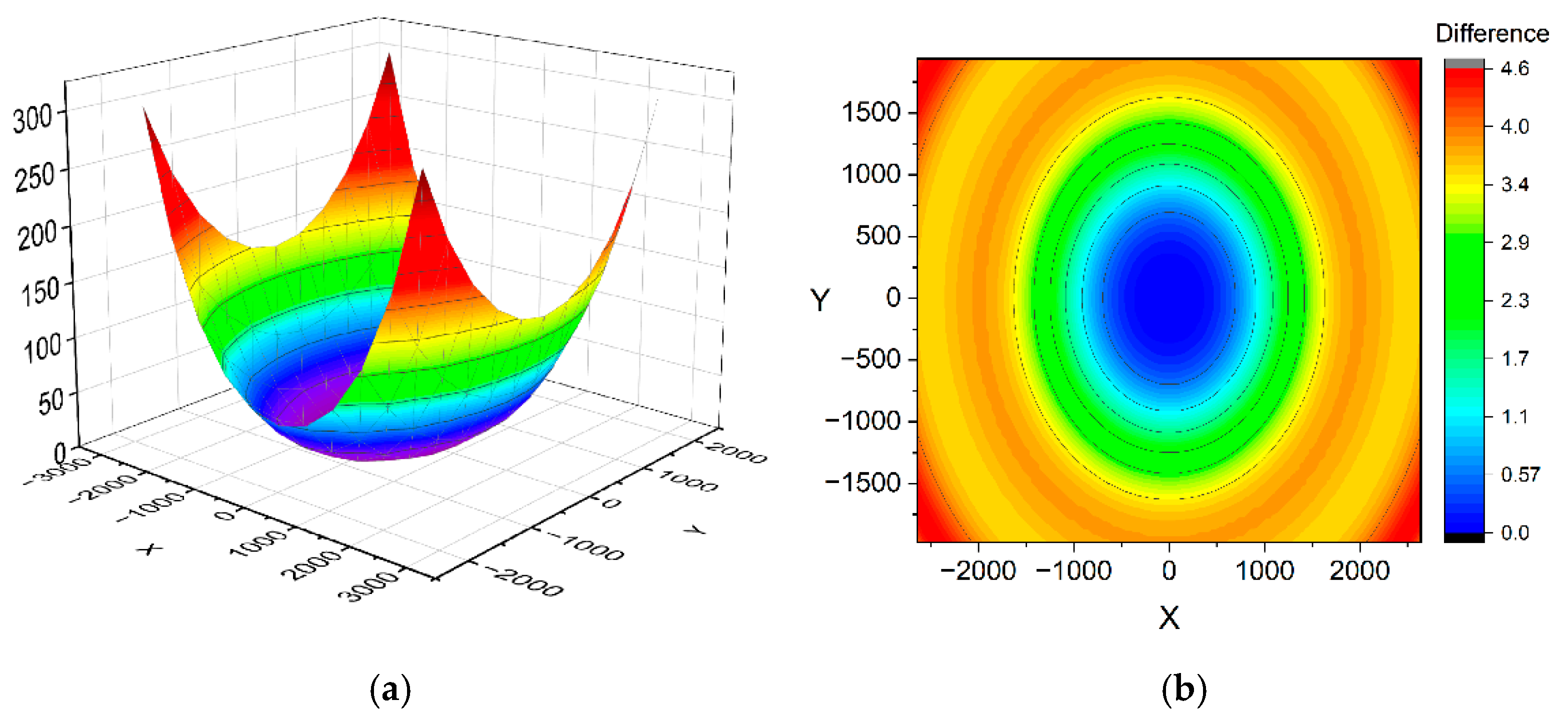
The scale ratio between the OI and distortion-corrected images increased by approximately 6.1–6.4% on average, with values of 1.061 for the calibrated IOPs and 1.064 for the manufacturer-provided IOPs, as shown in Table 6. The central region of the image showed almost no distortion, whereas the image corners exhibited maximum magnification values of approximately 21.2–21.5%. Figure 2a shows the spatial distribution of lens distortion in the OI acquired by the M3E. The distortion magnitude increased rapidly toward the image corners. Although slight numerical differences were observed between the two IOP sets, the overall distortion magnitude and spatial pattern were highly similar.

The average distortion magnitude was 64.242 pixels for the calibrated IOPs and 67.256 pixels for the manufacturer-provided IOPs. In both cases, radial distortion dominated the total lens distortion, whereas tangential distortion was negligible, with average values of 0.252 and 0.192 pixels, respectively. Figure 2b shows the spatial difference in lens distortion between the calibrated IOPs and the manufacturer-provided IOPs. The difference between the two distortion models had an average of 3.014 pixels, a maximum of 4.573 pixels, and a standard deviation of 1.149 pixels. The correlation coefficient between the two models was r = 0.9998, indicating that the two distortion patterns were nearly identical. The manufacturer-provided IOPs produced distortion values approximately 1.27% larger than those obtained from the calibrated IOPs, which can be considered a minor difference in practical terms. Additional altitude-wise calculations using image groups acquired at 120, 130, 140, and 150 m showed that the overall distortion magnitude was highly similar, with a maximum difference of approximately 1 pixel in total distortion. Because the same camera–lens system and near-nadir viewing geometry were used throughout the experiment, the estimated distortion parameters were considered reasonably consistent under the acquisition conditions of this study.

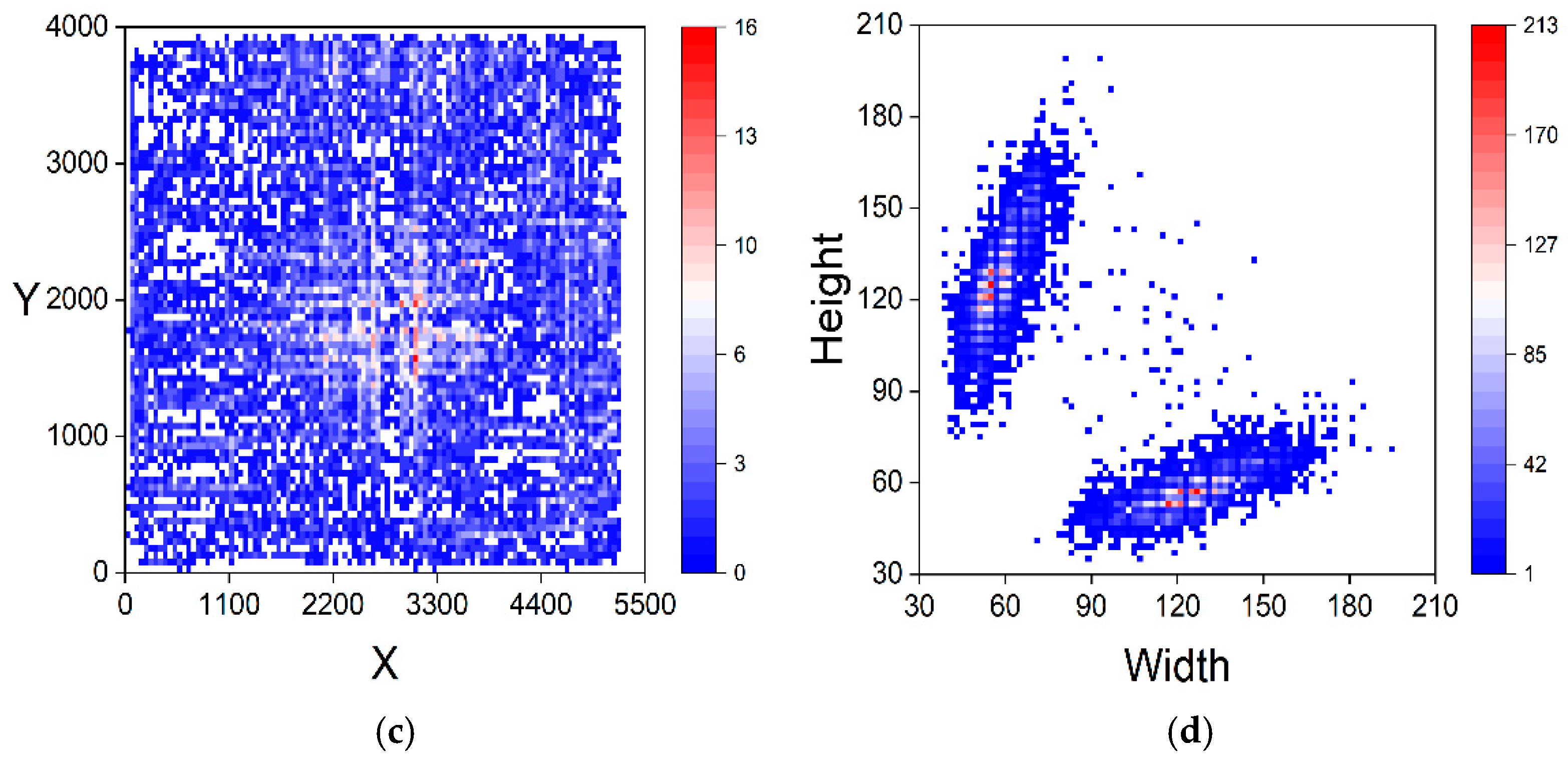
Figure 2c shows the spatial distribution of vehicle locations in the entire 5280 × 3956 pixel image. Vehicle locations were slightly concentrated near the image center. This pattern was caused by the selection of images in which vehicles occupied a sufficient portion of the frame. Figure 2d presents the object size distribution in the dataset. The distribution formed two major groups because the width and height of the annotated bounding boxes varied depending on the alignment of vehicle orientation with the X and Y axes of the image coordinate system.

The object size statistics for each image type are summarized in

Table 7. Vehicle bounding box size statistics by image preprocessing condition. (Unit: pixels).

Type	Vehicle Length		Vehicle Width		Width (X Axis)		Height (Y Axis)
	Average	Stdev	Average	Stdev	Average	Stdev	Average	Stdev
OI	126.520	16.160	57.967	7.507	90.852	35.637	93.635	37.328
MOI	127.397	15.887	58.270	7.407	91.493	35.827	94.174	37.541
Bilinear/Nearest	135.909	17.105	62.230	8.281	97.874	38.420	100.264	39.956
Total Average	129.849	16.919	59.448	7.973	93.337	36.759	95.960	38.384

. In Table 7, “vehicle length” and “vehicle width” represent the bounding-box dimensions defined along the vehicle direction, whereas “width (X axis)” and “height (Y axis)” represent the bounding-box dimensions measured in the image coordinate system. The aggregated mean object size ranged from 90 to 97 pixels in width and from 90 to 100 pixels in height. The average object size increased in the order of OI, MOI, and Bilinear/Nearest. Compared with OI, MOI showed an increase of approximately 0.6–0.7%, mainly because severely distorted peripheral regions were excluded. The Bilinear and Nearest images showed a 7.0–7.8% increase in object size due to lens distortion correction.

In this study, the small-object metrics AP_S and AR_S in the COCO evaluation were not considered. According to the COCO definition, an object is classified as small only when its area is less than 32² pixels [31]. However, none of the ground-truth vehicle instances in the study area satisfied this criterion. Therefore, the small-object metrics were not calculated and were reported as NaN or −1.000.

3.3. Comparison of Detection Accuracy Between Faster R-CNN and Cascade R-CNN

This section compares the detection performance of Faster R-CNN and Cascade R-CNN to evaluate the effect of detector architecture on UAV-based vehicle detection. According to Table 7, the directional vehicle dimensions in the OI, MOI, and distortion-corrected image datasets were approximately 58–62 pixels in width and 126–136 pixels in length. Based on these object sizes, the subsequent evaluation focused on AP and AR for all object sizes, medium objects, and large objects. Best denotes the checkpoint with the highest validation AP, whereas Final denotes the checkpoint obtained at the last training epoch.

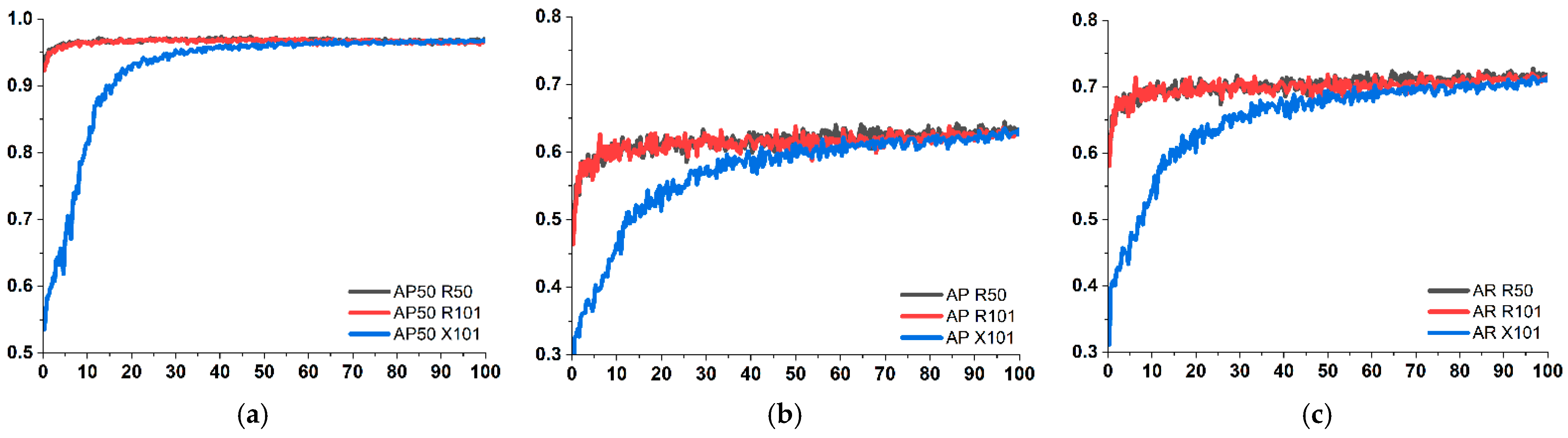
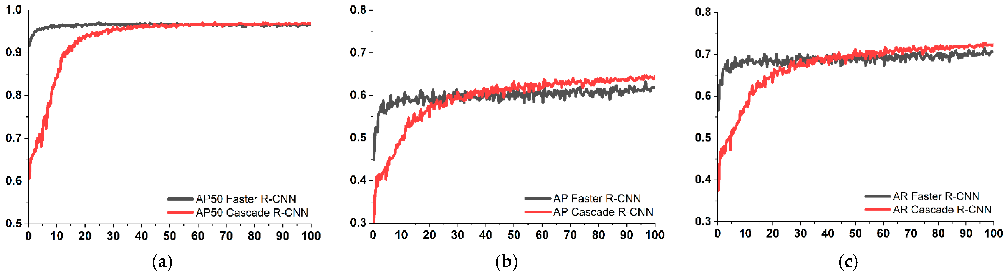
Following the COCO evaluation protocol, AP50, AP, and AR were compared between Faster R-CNN and Cascade R-CNN. Figure 3 shows the changes in AP50, AP, and AR over training epochs. In Figure 3a, Faster R-CNN showed higher AP50 values during the early training stage, whereas Cascade R-CNN gradually improved and reached a comparable level in the later stage. Similar trends are observed in Figure 3b,c. Faster R-CNN achieved slightly higher AP and AR values at the beginning of training, while Cascade R-CNN steadily improved and eventually surpassed Faster R-CNN toward the end of training.

Table 8. Detection performance comparison between Faster R-CNN and Cascade R-CNN at the best and final checkpoints.

Model	Stage	AP50	AP	AP_M	AP_L	AR	AR_M	AR_L
Faster R-CNN	Best	0.975	0.649	0.653	0.653	0.730	0.728	0.753
	Final	0.966	0.619	0.628	0.615	0.706	0.696	0.741
Cascade R-CNN	Best	0.976	0.662	0.663	0.671	0.739	0.735	0.758
	Final	0.968	0.644	0.646	0.651	0.724	0.717	0.752
Difference	Best	0.001	0.013	0.010	0.018	0.009	0.007	0.005
	Final	0.002	0.025	0.018	0.036	0.019	0.021	0.010

summarizes the detection performance of Faster R-CNN and Cascade R-CNN at the best and final checkpoints. At the best checkpoint, Cascade R-CNN showed slightly higher performance than Faster R-CNN across most metrics. In particular, Cascade R-CNN achieved AP and AR values of 0.662 and 0.739, respectively, compared with 0.649 and 0.730 for Faster R-CNN. The improvement was modest, with AP increasing by 0.013 and AR increasing by 0.009.

At the final checkpoint, the performance gap between the two detectors became more evident. Cascade R-CNN achieved AP and AR values of 0.644 and 0.724, whereas Faster R-CNN achieved 0.619 and 0.706, respectively. The largest improvement was observed in AP_L, where Cascade R-CNN exceeded Faster R-CNN by 0.036. Overall, Cascade R-CNN provided modest but consistent improvements over Faster R-CNN, particularly in AP and AP_L, although Faster R-CNN showed faster convergence during the early training stage.

3.4. Comparison of Detection Accuracy Across Backbone Architectures

This section compares the influence of backbone architecture on vehicle detection performance. Three backbone networks, R50, R101, and X101, were evaluated under the same experimental conditions. Figure 4 shows the changes in AP50, AP, and AR over training epochs for each backbone architecture. During the early training stage, R50 and R101 showed relatively higher AP and AR values than X101. However, X101 gradually improved as training progressed, and the performance gap among the three backbones became smaller in the later training stage.

Table 9. Detection performance comparison across three backbone networks at the best and final checkpoints.

Backbone	Stage	AP50	AP	AP_M	AP_L	AR	AR_M	AR_L
R50	Best	0.977	0.666	0.668	0.669	0.745	0.743	0.764
	Final	0.969	0.639	0.645	0.640	0.723	0.715	0.752
R101	Best	0.977	0.665	0.666	0.671	0.743	0.741	0.761
	Final	0.967	0.636	0.642	0.637	0.721	0.712	0.752
X101	Best	0.973	0.636	0.639	0.646	0.716	0.711	0.743
	Final	0.966	0.619	0.624	0.623	0.702	0.693	0.736

summarizes the detection performance of R50, R101, and X101 at the best and final checkpoints. At the best checkpoint, R50 and R101 showed nearly identical performance, with AP values of 0.666 and 0.665 and AR values of 0.745 and 0.743, respectively. In contrast, X101 showed lower AP and AR values of 0.636 and 0.716, indicating that the deeper and more complex backbone did not improve detection performance under the experimental conditions of this study.

At the final checkpoint, R50 maintained the highest overall performance, with AP and AR values of 0.639 and 0.723, respectively. R101 showed similar but slightly lower values, with AP and AR values of 0.636 and 0.721, respectively. X101 showed the lowest final performance among the three backbones, with AP50, AP, and AR values of 0.966, 0.619, and 0.702, respectively. This indicates that X101 did not provide an advantage over R50 or R101 in either loose-threshold detection performance or stricter COCO-style evaluation metrics.

Overall, R50 and R101 consistently outperformed X101 in AP and AR. The performance difference between R50 and R101 was small, but R50 showed slightly higher values in most metrics and required shorter training time. Therefore, R50 provided the most favorable balance between detection accuracy and training time among the three backbone architectures.

3.5. Effects of Lens Correction

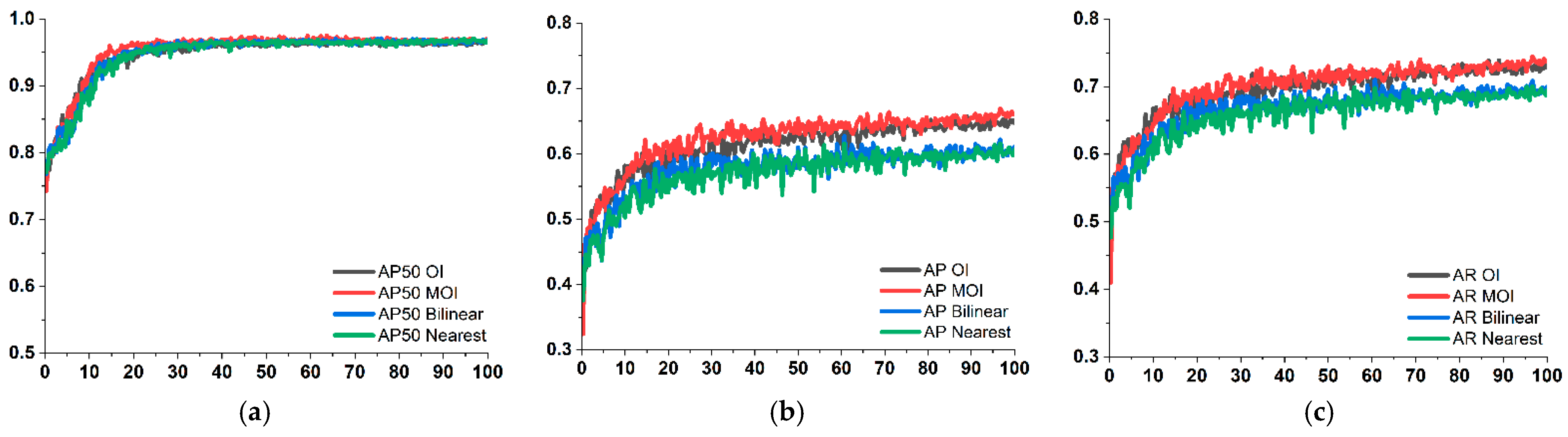
This section evaluates the effect of image preprocessing and lens correction on vehicle detection performance. The four image preprocessing conditions were OI, MOI, Bilinear, and Nearest. Figure 5 shows the changes in AP50, AP, and AR for the four image preprocessing conditions.

As shown in Figure 5a, AP50 values remained high for all image preprocessing conditions throughout training. However, clearer differences were observed in AP and AR, as shown in Figure 5b,c. OI and MOI generally maintained higher AP and AR values during training, whereas Bilinear and Nearest showed lower values after lens distortion correction.

Table 10. Detection performance comparison across image preprocessing conditions at the best and final checkpoints.

Image Type	Stage	AP50	AP	AP_M	AP_L	AR	AR_M	AR_L
OI	Best	0.973	0.670	0.674	0.671	0.749	0.750	0.756
	Final	0.967	0.647	0.653	0.639	0.728	0.725	0.747
MOI	Best	0.979	0.679	0.683	0.669	0.753	0.754	0.756
	Final	0.968	0.662	0.667	0.650	0.737	0.736	0.751
Bilinear	Best	0.975	0.640	0.640	0.655	0.721	0.715	0.758
	Final	0.969	0.611	0.616	0.623	0.700	0.686	0.745
Nearest	Best	0.975	0.634	0.634	0.652	0.716	0.709	0.753
	Final	0.965	0.607	0.611	0.620	0.695	0.680	0.743

summarizes the detection performance at the best and final checkpoints. MOI achieved the highest overall performance among the four image preprocessing conditions at both checkpoints. At the best checkpoint, MOI achieved the highest AP and AR values of 0.679 and 0.753, respectively. Compared with OI, MOI slightly improved AP, AP_M, AR, and AR_M, while AP_L was slightly lower and AR_L remained the same. At the final checkpoint, MOI also showed the highest AP and AR values of 0.662 and 0.737, respectively, compared with 0.647 and 0.728 for OI.

In contrast, Bilinear and Nearest showed lower AP and AR values than OI and MOI. At the final checkpoint, Bilinear achieved AP and AR values of 0.611 and 0.700, respectively, while Nearest achieved 0.607 and 0.695. Compared with OI, Bilinear showed relative AP and AR ratios of 0.944 and 0.962, whereas Nearest showed relative AP and AR ratios of 0.938 and 0.955. Because OI retained a larger peripheral image extent, differences between OI and the other preprocessing conditions may include the effect of peripheral-area exclusion. However, MOI, Bilinear, and Nearest were matched in valid scene extent and peripheral-object inclusion. Therefore, the higher AP and AR of MOI relative to Bilinear and Nearest cannot be attributed to the removal of difficult peripheral objects and instead indicate an adverse influence of geometric remapping and resampling on detection localization. Although Bilinear and Nearest showed AP50 values comparable to OI and MOI, their AP, AP_M, AP_L, AR, and AR_M values were generally lower. Between the two interpolation methods, Bilinear showed slightly higher AP and AR values than Nearest. The complete final-checkpoint results for all 24 experimental combinations are provided in Appendix A 

Table A1. Final checkpoint detection performance for all 24 experimental combinations.

Image Type	Model	Backbone	AP50	AP	AP_M	AP_L	AR	AR_M	AR_L
OI	Faster R-CNN	R50	0.971	0.634	0.642	0.620	0.716	0.712	0.736
		R101	0.969	0.636	0.647	0.614	0.724	0.719	0.748
		X101	0.959	0.635	0.647	0.618	0.721	0.718	0.735
	Cascade R-CNN	R50	0.974	0.674	0.676	0.678	0.752	0.750	0.768
		R101	0.960	0.675	0.679	0.675	0.757	0.755	0.767
		X101	0.968	0.625	0.627	0.629	0.698	0.695	0.729
MOI	Faster R-CNN	R50	0.975	0.659	0.663	0.641	0.734	0.732	0.750
		R101	0.957	0.628	0.640	0.609	0.709	0.705	0.738
		X101	0.971	0.665	0.672	0.642	0.745	0.745	0.756
	Cascade R-CNN	R50	0.966	0.694	0.697	0.688	0.766	0.767	0.766
		R101	0.968	0.684	0.687	0.677	0.758	0.758	0.761
		X101	0.971	0.641	0.643	0.643	0.711	0.708	0.737
Bilinear	Faster R-CNN	R50	0.962	0.582	0.595	0.589	0.677	0.660	0.732
		R101	0.970	0.582	0.600	0.577	0.678	0.663	0.722
		X101	0.969	0.624	0.628	0.641	0.715	0.702	0.753
	Cascade R-CNN	R50	0.970	0.646	0.645	0.665	0.730	0.719	0.769
		R101	0.976	0.641	0.637	0.663	0.724	0.710	0.769
		X101	0.966	0.590	0.591	0.603	0.676	0.662	0.724
Nearest	Faster R-CNN	R50	0.967	0.597	0.606	0.602	0.689	0.672	0.741
		R101	0.966	0.602	0.605	0.618	0.691	0.673	0.745
		X101	0.958	0.584	0.589	0.610	0.674	0.654	0.737
	Cascade R-CNN	R50	0.965	0.628	0.634	0.635	0.718	0.707	0.753
		R101	0.968	0.641	0.639	0.661	0.725	0.713	0.766
		X101	0.964	0.589	0.593	0.595	0.674	0.661	0.718

.

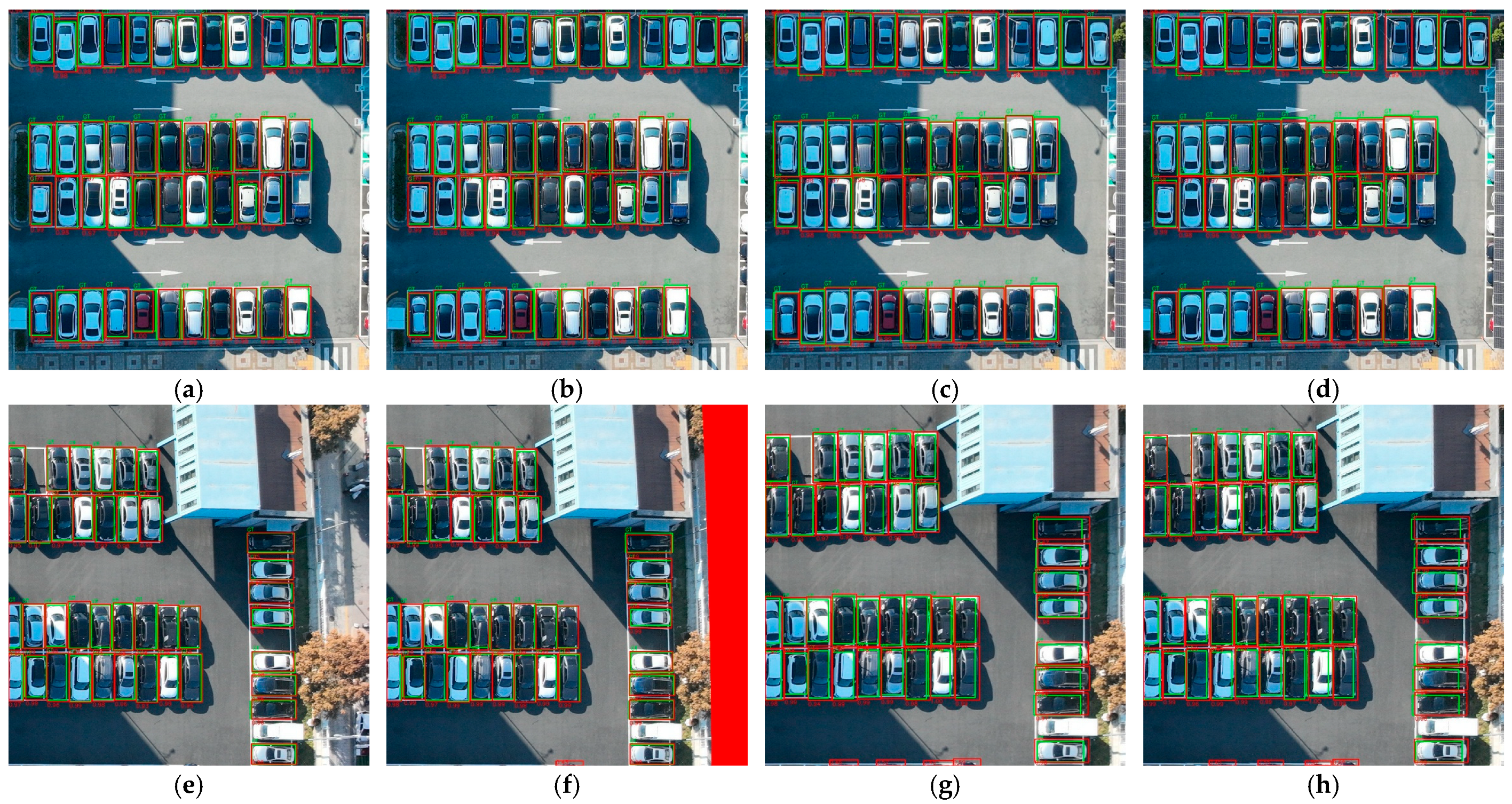
Figure 6 presents qualitative detection examples for central and peripheral image regions. The central region represents an area with relatively low lens distortion, whereas the peripheral region represents an area where lens distortion is more pronounced. In both regions, vehicles were generally detected across the four preprocessing conditions. However, differences in the overlap between ground-truth and predicted bounding boxes were visually observed among image types, especially when stricter localization quality is considered.

To quantitatively support the qualitative comparison, an object-level radial-zone analysis was conducted using Cascade R-CNN with R50. For this analysis, the center point of each ground-truth bounding box was used to calculate the normalized radial distance from the image center. The distance was normalized by the maximum possible distance from the image center to the image corner. Vehicle instances were grouped into three radial zones: center (0.00–0.33), middle (0.33–0.66), and edge/corner (0.66–1.00). Recall@0.50 was used as a lenient detection-success criterion, whereas Recall@0.75 was used as a stricter localization-quality criterion.

As shown in

Table 11. Radial-zone Recall@0.50 and Recall@0.75 for Cascade R-CNN with R50.

Image Type	Zone	GT Count	Recall@0.50	Recall@0.75
OI	Center	2181	0.988	0.937
	Middle	3059	0.992	0.952
	Edge/Corner	1539	0.992	0.916
MOI	Center	2179	0.985	0.934
	Middle	3012	0.991	0.953
	Edge/Corner	1138	0.989	0.936
Bilinear	Center	2173	0.989	0.870
	Middle	2777	0.994	0.900
	Edge/Corner	1208	0.988	0.885
Nearest	Center	2173	0.987	0.867
	Middle	2777	0.994	0.906
	Edge/Corner	1208	0.986	0.891

, Recall@0.50 remained consistently high across all preprocessing conditions and radial zones. This indicates that most vehicles were detected even in the edge/corner regions. However, clearer differences were observed under the stricter Recall@0.75 criterion. Bilinear and Nearest showed lower Recall@0.75 values than OI and MOI across the radial zones. Therefore, the lower AP values of the lens-corrected images were not primarily caused by complete detection failure but were more closely related to reduced bounding-box localization accuracy under stricter IoU criteria.

The radial-zone analysis also did not indicate a simple monotonic decrease in detection performance with increasing radial distance. This suggests that lens correction may reduce geometric distortion effects, but the accompanying geometric remapping and resampling process can reduce localization precision across the corrected images.

To further examine image degradation caused by lens correction, sharpness-based metrics and the Metashape image quality score were compared across the four preprocessing conditions, as summarized in

Table 12. Sharpness-based image quality metrics and Metashape image quality scores by image preprocessing condition.

Type	Variance of Laplacian		Tenengrad		Brenner		Sum of Modified Differences		Sum of Modified Differences 2		Metashape
	Avg	Stdev	Avg	Stdev	Avg	Stdev	Avg	Stdev	Avg	Stdev	Avg	Stdev
OI	0.561	0.105	1.105	0.190	0.039	0.008	0.123	0.017	0.080	0.016	0.963	0.037
MOI	0.619	0.122	1.158	0.218	0.041	0.009	0.125	0.018	0.084	0.018	0.978	0.040
Bilinear	0.318	0.068	0.883	0.170	0.030	0.007	0.104	0.016	0.061	0.013	0.954	0.038
Nearest	0.572	0.119	1.057	0.209	0.037	0.009	0.122	0.019	0.077	0.017	0.958	0.036

. MOI showed the highest values in most image quality metrics, whereas Bilinear showed the lowest values in most sharpness-based metrics. Compared with OI, Bilinear decreased by approximately 43.3% in Variance of Laplacian and 20.1% in Tenengrad, indicating that bilinear interpolation substantially reduced edge- and gradient-based sharpness. Nearest produced sharpness metric values closer to OI than Bilinear, with higher values than Bilinear in all sharpness-based metrics. However, the detection performance difference between Bilinear and Nearest was small, as shown in Table 10. This indicates that pixel-level sharpness differences did not translate directly into proportional differences in CNN-based detection performance. The Metashape image quality scores showed relatively small differences among all preprocessing conditions.

4. Discussion

The findings of this study primarily indicate that image preprocessing and lens distortion correction can substantially influence UAV-based vehicle detection performance. In the comparison between Faster R-CNN and Cascade R-CNN, Faster R-CNN showed relatively strong performance during the early training stage, whereas Cascade R-CNN gradually improved and achieved higher AP and AR values at both the best and final checkpoints. This tendency is consistent with the intrinsic design of the Cascade R-CNN framework, which progressively applies stricter IoU thresholds through multiple detection heads and iteratively refines bounding boxes [29].

The comparison of backbone architectures showed that R50 and R101 produced similar detection performance, whereas X101 showed relatively lower AP, AR, and AP50 values at the final checkpoint. This indicates that the deeper and more complex X101 backbone did not provide a performance advantage under the experimental conditions of this study. In general, deeper or more complex backbones can improve feature representation, but they also increase computational cost and memory demand. Previous studies have reported that object detection performance can vary depending on dataset characteristics, detector architecture, and backbone configuration [30]. In this study, R50 provided a favorable balance between detection accuracy and training time, indicating that increasing backbone complexity did not necessarily improve UAV-based vehicle detection performance.

The effect of image preprocessing was also clearly observed. MOI achieved the highest overall detection performance, followed by OI, Bilinear, and Nearest. MOI was generated by cropping the original images to match the effective field of view of the lens-corrected images, without applying geometric remapping or interpolation. This process removed severely distorted peripheral regions while preserving the original pixel structure. In contrast, Bilinear and Nearest were generated through lens distortion correction and interpolation-based remapping. Although lens distortion correction can improve geometric consistency, it can also introduce resampling artifacts, edge smoothing, blur, and partial loss of peripheral information. These effects can negatively affect the preservation of object boundaries, which are critical for accurate vehicle localization in UAV imagery. This result is consistent with previous studies suggesting that distortion and image rectification can affect downstream computer vision performance by altering object geometry, semantic context, and local image information [34,35].

The lower performance of Bilinear and Nearest compared with OI and MOI suggests that the main factor reducing detection accuracy was not simply the choice of interpolation method, but the lens correction and remapping process itself. Lens correction requires geometric transformation and pixel resampling, which can weaken high-frequency components, local edge details, and object boundaries. Interpolation, downsampling, and boundary handling during image warping may further reduce edge sharpness or introduce aliasing artifacts [36,37,38]. Therefore, even when lens correction improves geometric alignment, it may reduce the image details required for accurate object localization.

The radial-zone Recall@0.50 and Recall@0.75 analysis further supports this interpretation. Although Bilinear and Nearest maintained high Recall@0.50 values across radial zones, their Recall@0.75 values were consistently lower than those of OI and MOI. This indicates that the performance degradation of lens-corrected images was not mainly due to complete detection failure, but rather to reduced bounding-box localization precision under stricter IoU thresholds. The radial-zone analysis also showed that this decrease was not limited only to the most peripheral regions, suggesting that geometric remapping and resampling affected localization accuracy across the corrected images.

The comparison between Bilinear and Nearest provides an additional interpretation of the relationship between image quality metrics and object detection performance. The sharpness-based image quality metrics showed noticeable differences between the two interpolation methods, whereas their AP and AR values were similar. This indicates that pixel-level differences captured by sharpness metrics do not necessarily lead to proportional differences in CNN-based object detection performance. The sharpness metrics used in this study, including Variance of Laplacian, Tenengrad, Brenner, and SMD/SMD2, mainly quantify low-level image characteristics such as local intensity differences, gradient responses, edge strength, and high-frequency components [16,17,18,19]. Bilinear interpolation estimates new pixel values using a weighted average of neighboring pixels, which can produce smoother images but may suppress high-frequency details. Nearest-neighbor interpolation preserves original pixel values by assigning the closest input pixel value, but it can introduce jagged edges or aliasing artifacts. These differences can be strongly reflected in sharpness metrics.

However, CNN-based object detectors do not evaluate images only through pixel-level intensity differences. Instead, they learn hierarchical feature representations through convolutional operations, including object shape, boundary structure, texture, and spatial arrangement [39]. Therefore, even when Bilinear and Nearest images differ at the pixel level, the learned features may remain similar if the overall vehicle shape and spatial structure are preserved. In addition, convolution, stride, pooling, and feature aggregation operations progressively integrate information over broader spatial regions, which may reduce the influence of small local differences introduced by interpolation. This explains why Bilinear and Nearest showed relatively large differences in sharpness-based image quality metrics but only minor differences in AP and AR.

The performance difference between OI and MOI may partly reflect the exclusion of peripheral regions and objects because OI retained the full original image extent. However, this explanation does not apply to the comparison between MOI and Bilinear/Nearest. These three preprocessing conditions were constructed using the same valid scene extent and the same peripheral-object inclusion conditions. Therefore, the higher performance of MOI relative to Bilinear and Nearest cannot be explained by the removal of difficult boundary objects. Instead, the difference is more plausibly associated with the geometric remapping, local scale modification, interpolation, and resampling introduced during lens distortion correction.

This study has several limitations. First, the experiments were conducted using UAV images acquired from a single campus environment with the same UAV camera system. Second, the images were collected over two acquisition dates under relatively similar urban background conditions. Third, an independent external test site was not included. Therefore, the results should be further validated using additional study areas, UAV platforms, camera models, and flight conditions.

Overall, these results indicate that lens distortion correction should not be evaluated only from the perspective of geometric correction. For UAV-based vehicle detection, preserving object boundaries, local edge information, and useful contextual information can be as important as correcting lens distortion. Therefore, the effects of preprocessing should be interpreted jointly in terms of image quality characteristics and downstream detection performance, particularly when wide-angle UAV imagery is used for detecting small and regularly shaped objects such as vehicles.

5. Conclusions

This study evaluated the effects of lens distortion correction and image preprocessing on UAV-based vehicle detection. Four preprocessing conditions, OI, MOI, Bilinear, and Nearest, were compared using two detection models and three backbone architectures under 24 experimental conditions.

MOI achieved higher AP and AR than Bilinear and Nearest under the same valid scene extent and peripheral-object inclusion conditions. This result indicates that preserving the original pixel values within the valid image extent was more favorable for vehicle detection than applying lens-distortion remapping and interpolation under the tested conditions. Comparisons involving OI should be interpreted separately because OI retained the full original image extent and additional peripheral objects.

The image quality analysis showed that sharpness-based metrics and object detection metrics did not always respond consistently. Although Bilinear and Nearest differed noticeably in sharpness-based metrics, their AP and AR values were similar. This indicates that preprocessing strategies should be evaluated based on downstream detection performance rather than visual or sharpness-based image quality alone. As supporting results, Cascade R-CNN showed slightly better performance than Faster R-CNN, and R50 provided the most favorable balance between detection accuracy and training time.

Overall, this study demonstrates that geometric correction and object detection performance can involve a trade-off in wide-angle UAV imagery. Therefore, preprocessing strategies should be selected according to the final application objective rather than applying lens distortion correction automatically. Future studies should include additional study areas, different UAV platforms and camera models, and further object-level comparisons to verify the robustness and generalizability of the findings.