Comparative Performance Analysis of Mainstream Deep Learning and Vision Foundation Models for Small-Sample Vegetation Segmentation in High-Resolution Remote Sensing Imagery

Highlights

What are the main findings?

• Fine-tuned foundation models, especially SAM2.1-Tiny and SAM2-Tiny, achieved the best vegetation segmentation performance under small-sample high-resolution remote sensing conditions, with SAM2.1-Tiny reaching an mIoU of 0.7821 on the Zijinshan dataset and the strongest cross-dataset robustness.
• The proposed CT-PLST strategy effectively exploited cross-temporal unlabeled imagery and improved SAM2-Tiny from 0.7776 to 0.7888, confirming that high-confidence pseudo-label self-training can further reduce boundary omissions and improve stability.

What are the implications of the main findings?

• For practical remote sensing vegetation mapping, foundation models should be prioritized when segmentation accuracy and boundary completeness matter, while lightweight SAM variants are better suited to resource-constrained deployment.
• Cross-temporal self-training provides a low-cost way to use unlabeled seasonal imagery, reducing annotation demand and improving vegetation monitoring and change analysis in complex real-world scenes.

Abstract

Accurate extraction of vegetation information from high-resolution remote sensing (RS) imagery is crucial for efficient urban ecological environment monitoring and land use management. However, due to the high cost of manual annotation in remote sensing imagery and the complex textural variations and spectral confusion exhibited by vegetation under different terrains and lighting conditions, precise vegetation segmentation under small-sample conditions remains a significant challenge. Using the Nanjing Zijinshan region as a case study, this research conducts a systematic comparison of eight representative models within a unified high-resolution remote sensing small-sample experimental framework to address these complexity challenges. We fine-tuned and systematically compared the recently prominent “Segment Anything Model” (SAM) series (including SAM2-Tiny, SAM2.1-Tiny, MobileSAM, and MobileSAMV2), along with classic fully supervised models (U-Net, DeepLabV3+), open-vocabulary segmentation models (SegEarth-OV), and instance segmentation models (YOLO11s-seg), helping clarify the performance boundaries and applicable conditions of different technical paradigms in vegetation segmentation. Experimental results highlight the distinctive performance characteristics of these models. Notably, fine-tuned vision foundation models (such as SAM2.1-Tiny and SAM2-Tiny) demonstrated superior segmentation performance and cross-dataset generalization capabilities, with SAM2.1-Tiny achieving the highest mean Intersection over Union (mIoU; 0.7821) on the Zijinshan dataset, a 5.5% improvement over the classic U-Net model; SAM2-Tiny also maintained the most stable generalization performance in cross-dataset testing on LoveDA, Potsdam, and Vaihingen. In contrast, zero-shot SegEarth-OV and instance segmentation model YOLO11s-seg showed relatively lower performance in current semantic segmentation tasks, revealing the application boundaries of different paradigms. Beyond these findings, to further leverage unlabeled temporal imagery and break through small-sample constraints, we propose an innovative Cross-Temporal Pseudo-Label Self-Training (CT-PLST) strategy, which successfully improved SAM2-Tiny’s mIoU from 0.7776 to 0.7888 (+1.44%), providing a low-cost efficiency enhancement solution for remote sensing segmentation under scarce annotation conditions. To promote reproducible research in remote sensing and computer vision, we publicly release the fine-tuned models, related comparative experiment code, and a high-resolution remote sensing vegetation dataset covering multi-temporal scenarios; access details are provided in the Data Availability Statement. The findings of this study, combined with the proposed CT-PLST strategy and the high-precision segmentation results achieved by vision foundation models, can strongly support tracking analysis of vegetation cover changes, urban heat island effect assessment, and exploration of ecosystem dynamic evolution. Meanwhile, these achievements also provide valuable theoretical guidance and engineering references for practitioners and researchers in finding lightweight segmentation models suitable for specific image characteristics and computational cost constraints in practical applications such as rapid disaster risk assessment or forestry resource surveys.

1. Introduction

Vegetation plays a fundamental role in carbon cycling, local climate regulation, urban heat island mitigation, and biodiversity maintenance [1,2,3]. Therefore, its boundary delineation and spatial distribution extraction are directly related to applications such as urban ecological assessment, land use/cover change monitoring, forest phase analysis, and precision agriculture [4,5,6]. High-resolution remote sensing (RS) imagery can provide more detailed canopy texture and ground object boundary information and has become an important data source for vegetation remote sensing research [7,8]. With the popularization of commercial satellites and unmanned aerial vehicle (UAV) platforms, the cost of acquiring high-resolution near-ground or aerial imagery continues to decrease, but higher spatial detail also means stronger inter-class confusion and boundary uncertainty [9,10,11,12].

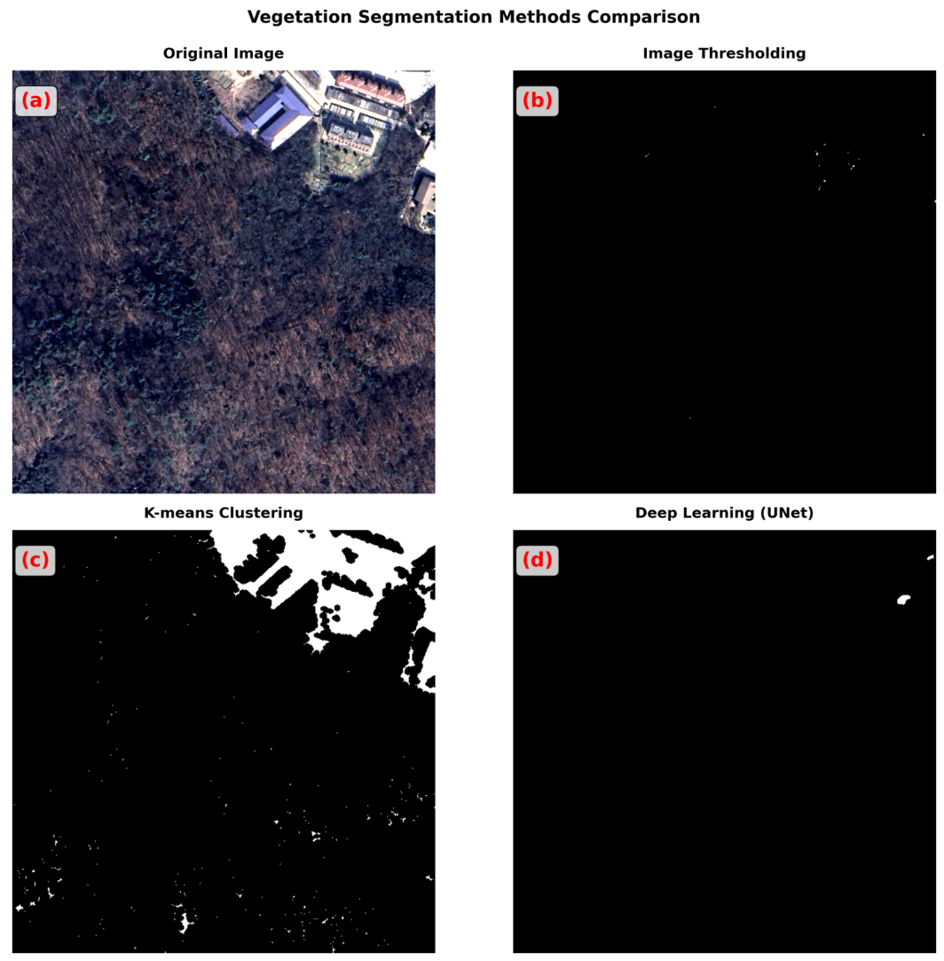
However, this also significantly increases the difficulty of automatically extracting target features. Traditional classification algorithms based on spectral features (such as Normalized Difference Vegetation Index (NDVI), threshold methods based on hue–saturation–value (HSV) color space, and clustering) perform reasonably well when facing simple backgrounds and images with significant spectral differences at medium to low resolutions. However, when applied to high-resolution imagery, due to the intensification of “same object different spectrum” and “different object same spectrum” phenomena, the boundaries between vegetation and non-vegetation ground objects become blurred, and the segmentation accuracy and robustness of traditional methods significantly decline [13,14,15]. In recent years, deep learning (DL) technologies represented by deep convolutional neural networks (CNNs) have demonstrated powerful multi-level feature learning and pattern recognition capabilities, achieving breakthrough progress in the field of remote sensing semantic segmentation [16,17,18,19]. For example, the classic U-Net [20] and DeepLabV3+ [21], which incorporates atrous spatial pyramid pooling modules, can significantly surpass the segmentation effects of classic image processing algorithms when sufficient high-quality manually annotated pixel-level training data is obtained (as shown in Figure 1).

Although fully supervised deep learning models have shown excellent performance in vegetation extraction tasks, their practical applications still face obvious bottlenecks [22,23]. On one hand, pixel-level manual annotation of remote sensing imagery is an extremely time-consuming and expensive task, especially in dynamic monitoring tasks involving multi-temporal and multi-scale scenarios, making it extremely difficult to construct a sufficiently large high-quality annotation library [24,25]. If training is conducted directly under data scarcity (i.e., “small-sample”) conditions, the above-mentioned fully supervised models with large parameters are highly prone to severe overfitting, leading to a cliff-like decline in cross-regional or cross-domain generalization capabilities [26,27]. Recent few-shot remote sensing benchmarks further show that limited labeled data remain a central obstacle for robust semantic segmentation, especially when models must preserve both base-class performance and adaptation to new land-cover patterns [28]. Therefore, reducing annotation dependence requires not only stronger segmentation architectures but also more efficient use of the available training data. Existing studies have addressed this issue along two related lines. One line focuses on selecting more representative training samples; for example, grouped sample selection in multispectral remote sensing classification can improve accuracy with fewer labeled samples [29]. Another line focuses on dataset quality control for deep CNN training, where low-quality or weakly informative samples are filtered to improve learning efficiency without sacrificing accuracy [30]. These studies indicate that the composition and reliability of the training set are especially important when high-resolution annotations are limited. In the present study, this idea is extended to cross-temporal vegetation segmentation by using confidence-filtered pseudo-labels from unlabeled temporal imagery to enlarge the effective supervision set while controlling label noise.

To address the data scarcity crisis brought by small-sample annotation, vision foundation models have entered the research horizon as a completely new technical paradigm [31]. In 2023, Meta AI released the “Segment Anything Model” (SAM) [32], which, through pre-training on the massive real-world Segment Anything 1 Billion (SA-1B) dataset, demonstrated unprecedented zero-shot and few-shot segmentation potential. Subsequently, to overcome the high computational overhead of the original SAM, lightweight foundation networks and derivative structures, including MobileSAM [33], SAM2-Tiny [34], and the updated SAM2.1 were successively proposed, further improving inference efficiency on edge devices and scene segmentation performance [35,36,37]. Recent studies have also explored how SAM-type foundation models can be adapted to remote sensing semantic segmentation through object/boundary constraints, multimodal adapters, and lightweight geospatial-domain initialization for onboard deployment [38,39,40]. Additionally, open-vocabulary segmentation models such as SegEarth-OV [41] attempt to break free from the burden of heavy pixel annotation through cross-modal text prompts, while recent open-vocabulary remote sensing segmentation research has further highlighted the need to combine general vision–language priors with remote sensing domain features [42]. The latest instance segmentation architecture of the YOLO series, YOLO11s-seg, combines multi-target localization with pixel-level instance mask extraction [43].

Although these novel deep learning architectures and vision foundation networks have demonstrated impressive results on their respective domains’ standard benchmarks, for the vertical task of vegetation segmentation in high-resolution remote sensing imagery under “small-sample” extreme conditions, the academic community still lacks comprehensive and in-depth systematic comparative evaluation [44,45,46]. Specifically, what are the performance limits of different paradigms (foundation models vs. fully supervised models vs. open-vocabulary models vs. instance segmentation models) under small-sample constraints? Are there systematic differences in their generalization capabilities when facing cross-regional public remote sensing datasets with different lighting and climate characteristics? More importantly, how can we efficiently and cost-effectively utilize the abundant unlabeled image resources in temporal remote sensing data to further improve the small-sample learning effects of foundation models? These urgent real-world questions still lack quantitative verification and scientific conclusions [47,48,49,50].

To fill the above research gaps and solve the small-sample application dilemma in vegetation monitoring, this study uses high-resolution red–green–blue (RGB) remote sensing imagery (0.75 m resolution) from the Nanjing Zijinshan region from 2022 to 2024 as the core test platform, systematically evaluating and comparing the performance of eight currently highly representative deep learning networks in small-sample vegetation segmentation tasks. These eight networks cover fine-tuned vision foundation model series (SAM2-Tiny, SAM2.1-Tiny, MobileSAM, MobileSAMV2), classic feature encoding–decoding fully supervised models (UNet, DeepLabV3+), open-vocabulary segmentation models (SegEarth-OV), and efficient instance segmentation models (YOLO11s-seg).

The cross-dataset comparisons in this study are not intended to serve as dataset-independent leaderboard results alone, because the mean Intersection over Union (mIoU) depends on sensor characteristics, spatial resolution, geographic domain, annotation style, and acquisition conditions. Instead, they are used to examine how different model paradigms respond to realistic domain shifts after being trained under the same small-sample vegetation segmentation protocol. The key distinction of this research is therefore the combination of a self-constructed multi-temporal Zijinshan vegetation dataset, a unified training and inference setting, cross-domain robustness testing, and Cross-Temporal Pseudo-Label Self-Training (CT-PLST) with unlabeled temporal imagery under scarce annotation conditions.

Based on the above motivations, the main research contributions of this paper can be summarized by the following four aspects:

• Systematic Model Comparison Innovation: This study comprehensively compares eight mainstream models within a unified high-resolution remote sensing small-sample experimental framework, covering vision foundation models (SAM2 series, MobileSAM series), classic fully supervised models, open-vocabulary models, and instance segmentation models, and clarifies the performance boundaries and applicable conditions of different paradigms in vegetation segmentation under small-sample constraints [51,52,53,54,55].
• Vision Foundation Model Generalization Verification: In a high-resolution remote sensing small-sample environment, this study systematically shows that fine-tuned SAM2.1-Tiny and SAM2-Tiny achieve optimal accuracy, the strongest stability, and the best cross-dataset generalization capability in vegetation segmentation. Cross-validation on three public remote sensing datasets (LoveDA, Potsdam, Vaihingen) provides strong quantitative evidence for the practical application of foundation models and offers an evidence-based model selection basis for researchers [56,57,58,59,60].
• Cross-Temporal Pseudo-Label Self-Training Strategy Innovation: Addressing the reality of scarce remote sensing annotations and abundant multi-temporal data, we propose the CT-PLST method. This innovative strategy effectively utilizes unlabeled temporal imagery to improve model performance, increasing SAM2-Tiny’s mIoU from 0.7776 to 0.7888 (+1.44%), providing a low-cost efficiency enhancement solution for small-sample remote sensing tasks and revealing the practical role of temporal self-supervision in alleviating annotation scarcity [61,62,63,64,65].
• Open-Source Dataset and Engineering Guidance: We construct and open-source the Nanjing Zijinshan multi-temporal high-resolution vegetation segmentation dataset while publicly releasing the complete set of fine-tuned models, comparative experiment code, and model configurations. We provide lightweight deployment recommendations from multiple dimensions including accuracy, speed, resource consumption, and stability, offering directly implementable engineering references for practical tasks such as ecological monitoring and forestry surveys, significantly improving research transparency and application accessibility in this field [66,67].

The remainder of this paper is organized as follows. Section 2 presents the materials and methods. Section 3 describes the experimental setup and results. Section 4 discusses the model differences, CT-PLST, and practical implications. Finally, Section 5 summarizes the main findings, limitations, and future research directions.

2. Materials and Methods

2.1. Deep Learning Segmentation Models

Feature extraction is the cornerstone of modern remote sensing image semantic segmentation tasks. In this study, eight representative models were selected to cover classical fully supervised semantic segmentation, lightweight vision foundation models, open-vocabulary segmentation, single-stage instance segmentation, and fine-tuned foundation model paradigms. These models were evaluated under the same dataset split, image size, training protocol, and metric system to ensure a fair comparison. Their main architectural characteristics, technical paradigms, and task-specific roles are summarized in

Table 1. Summary of the deep learning and foundation segmentation models compared in this study.

Model	Paradigm	Main Architectural Characteristic	Role in This Study
U-Net [2]	Fully supervised semantic segmentation	Symmetric encoder–decoder with skip connections	Classical baseline for evaluating pixel-level vegetation segmentation under limited annotations.
DeepLabV3+ [8]	Fully supervised semantic segmentation	Atrous Spatial Pyramid Pooling with encoder–decoder refinement	Baseline for assessing multi-scale context modeling in vegetation patches of different sizes.
MobileSAM [15]	Lightweight vision foundation model	Distilled Vision Transformer (ViT)-Tiny image encoder with a Segment Anything Model (SAM)-style prompt decoder	Lightweight foundation-model baseline for balancing segmentation accuracy and computational cost.
MobileSAMV2 [14]	Lightweight vision foundation model	Enhanced multi-scale feature interaction and mask refinement	Improved lightweight variant for testing whether stronger feature fusion benefits complex vegetation boundaries.
YOLO11s-seg [25]	Single-stage instance segmentation	Joint object detection and prototype-based mask reconstruction	Instance-segmentation reference for evaluating its suitability for continuous vegetation mask extraction.
SegEarth-OV [26]	Open-vocabulary segmentation	Contrastive Language–Image Pre-training (CLIP)-based image–text alignment and prompt-driven inference	Zero-shot reference for testing whether text-guided segmentation can replace task-specific supervision.
SAM2-Tiny [12]	Vision foundation model fine-tuning	Hiera hierarchical image encoder with lightweight mask decoding	Foundation-model baseline for few-shot fine-tuning and cross-dataset generalization analysis.
SAM2.1-Tiny [14]	Updated vision foundation model fine-tuning	Refined SAM2-Tiny architecture with improved convergence behavior	Main high-performing foundation model used to evaluate accuracy, stability, and generalization.

.

In addition to the eight models used in the main controlled comparison, four recent foundation- and prompt-based models were evaluated as supplementary experiments to broaden the model scope. DINOv2 ViT-L/14-Reg and DINOv3 ViT-L/16 were tested as frozen-backbone dense segmentation models with lightweight trained segmentation heads, reflecting the recent progress of self-supervised visual foundation backbones with dense feature transferability [68,69]. QwenVL2.5-3B and LocateAnything-3B were evaluated separately as prompt-based localization or grounding models; their predicted boxes were converted into coarse binary masks only for box-mask metric calculation. The inclusion of QwenVL2.5-3B follows recent progress in vision–language models with structured localization ability [70]. Therefore, these two prompt-based models are reported as supplementary evidence rather than as direct replacements for dense semantic segmentation networks.

2.2. Vegetation Segmentation Strategy Using Deep Learning Models

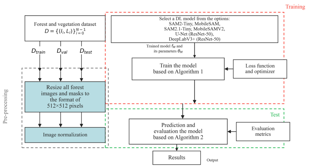
Based on the aforementioned models, this study deploys a systematic experimental diagnostic workflow including data flow slicing, fine-tuning strategy configuration, and cross-domain inference generalization (with the overall system structure shown in Figure 2).

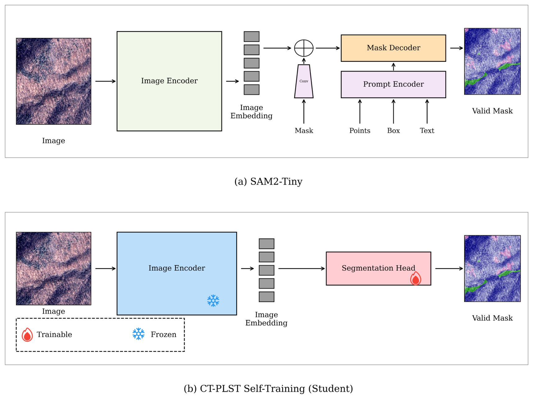
In standard DL segmentation processes, extremely small amounts of manually annotated data (small-sample constraints) cause all models, even fully supervised networks’ backbones, to exhibit severe overfitting effects and statistical bias phenomena. To break through this constraint, this section focuses on explaining the core innovative method of this paper: the Cross-Temporal Pseudo-Label Self-Training (CT-PLST) mechanism. This method addresses the reality of high remote sensing image annotation costs but abundant multi-temporal data, innovatively designing a teacher–student distillation framework that significantly improves foundation model segmentation accuracy driven by extremely small amounts of annotations while maintaining high confidence by effectively activating massive unlabeled temporal image resources in the same region, providing a low-cost, high-efficiency enhancement solution for small-sample remote sensing tasks (workflow shown in Figure 3) [27,31].

The CT-PLST mechanism is designed as a rigorous teacher–student two-stage distillation process. Let ${\mathcal{D}}_L=\left\{(x_i,y_i)\right\}$ represent the labeled dataset containing extremely small amounts of accurately annotated historical imagery (e.g., 2022–2023), and let ${\mathcal{D}}_U=\left\{x_j\right\}$ represent massive unlabeled new temporal long-scroll remote sensing data (e.g., 2024).

Stage 1: Teacher Model Optimal Fitting and Label Inference.

On the foundation backbone (such as fine-tuned SAM2-Tiny, etc.), iterative supervised learning is performed through the labeled dataset ${\mathcal{D}}_L$ to obtain the “teacher model weights” $f_{\mathrm{Teacher}}$ at the peak validation set accuracy. Subsequently, $f_{\mathrm{Teacher}}$ is used to perform frame-by-frame forward inference on the massive unlabeled set ${\mathcal{D}}_U$, generating prediction posterior probability distribution matrices $P_j$ containing classification confidence. To eliminate pseudo-artifacts from mis-segmentation, we use confidence threshold $\tau$ to filter pseudo-labels; combining threshold ablation results, this paper finally sets $\tau$ to 0.70 as the default setting for CT-PLST:

Here, $\tau$ is a pseudo-label confidence threshold rather than the ordinary 0.5 probability cutoff used for final binary mask generation during unified inference. Its value was selected according to three criteria: retaining enough temporal samples for self-training, suppressing low-confidence boundary and shadow errors, and achieving the best performance trade-off in the threshold ablation. This confidence-based filtering is consistent with common semi-supervised segmentation practice, where high-confidence predictions are treated as reliable pseudo-labels, whereas low-confidence or unreliable predictions are suppressed, separated, or purified before being used for training [32,71,72]. Multi-threshold image binarization is widely used in remote sensing when vegetation or other land-cover classes are separated from spectral indices or grayscale response maps. In CT-PLST, however, thresholding is applied to model posterior confidence to control pseudo-label reliability, so the threshold is determined by pseudo-label quality and ablation performance rather than by the histogram distribution of raw image intensities.

$${\widehat{y}}_j\left(k\right)=\left\{\begin{array}{cc}c\hfill & \mathrm{if}{P}_{j,c}\left(k\right)>\tau \hfill \\ \mathrm{ignore}\hfill & \mathrm{otherwise}\hfill \end{array}\right.$$

(1)

where $P_{j,c}\left(k\right)$ represents the predicted probability that the k-th pixel of the j-th unlabeled image belongs to class c (e.g., vegetation or not). Only when the probability breaks through the $\tau$ threshold can it be legally converted to a deterministic strong pseudo-class ${\widehat{y}}_j$.

Stage 2: Student Network Retraining Joint Iteration.

We forcibly bind the extracted high-quality pseudo-label set ${\tilde{\mathcal{D}}}_U=\left\{(x_j,{\widehat{y}}_j)\right\}$ with the gold standard set ${\mathcal{D}}_L$ for joint training iteration (retraining) by the pre-initialized “student model” $f_{\mathrm{Student}}$. In this joint cycle, the student model’s generalization ability is greatly enhanced due to constraints from expanded multi-temporal physical geomorphological features [32,34]. The overall constraint loss function used for end-to-end network iteration is

$${\mathcal{L}}_{\mathrm{total}}={\mathcal{L}}_{\mathrm{ce}}(f_{\mathrm{Student}}\left(x_i\right),y_i)+\lambda ·{\mathcal{L}}_{\mathrm{ce}}(f_{\mathrm{Student}}\left(x_j\right),{\widehat{y}}_j)$$

(2)

where ${\mathcal{L}}_{\mathrm{ce}}(·)$ adopts standard pixel-level cross-entropy loss to separately calculate the distance deviation between the supervised component and teacher-specified labels. This paper fixes $\lambda$ at 1.0; i.e., the supervised term and pseudo-label term adopt equal-weight fusion to prevent the unsupervised branch from excessively dominating optimization in early training.

2.3. Dataset

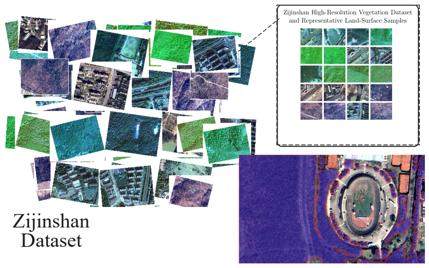
To evaluate the model and the proposed self-training framework’s high-resolution generalization capability, this study uses one self-constructed multi-temporal dataset and three public remote sensing semantic segmentation datasets. The Zijinshan dataset serves as the core few-shot training and same-domain temporal testing dataset, while LoveDA, Potsdam, and Vaihingen are used for cross-dataset robustness assessment under different spatial resolutions, urban structures, and vegetation–background distributions. Representative samples from the Zijinshan dataset are shown in Figure 4, and the main dataset characteristics are summarized in

Table 2. Summary of the datasets used in this study.

Dataset	Coverage and Data Source	Resolution/Image Setting	Role in This Study
Zijinshan	Nanjing Zijinshan Scenic Area and surrounding urban–rural interface; self-constructed red–green–blue (RGB) dataset annotated using the Computer Vision Annotation Tool (CVAT)	0.75 m/pixel; 512 × 512 patches; 201 images from 2022 to 2024	Self-constructed dataset for few-shot training, validation, same-domain testing, and Cross-Temporal Pseudo-Label Self-Training (CT-PLST). The 2022–2023 images provide 134 labeled samples, and the 2024 images provide 67 temporal test samples.
LoveDA [48]	Public urban–rural remote sensing dataset covering scenes from Nanjing and Changzhou	0.3 m spatial resolution	Cross-dataset test for complex urban–rural mixtures, building shadows, and vegetation-background confusion.
Potsdam [51]	International Society for Photogrammetry and Remote Sensing (ISPRS) Potsdam aerial benchmark dataset from Germany	0.05 m spatial resolution	Cross-dataset test for ultra-high-resolution urban scenes with regular green spaces, buildings, and fine boundary details.
Vaihingen [50]	ISPRS Vaihingen aerial benchmark dataset from Germany	0.09 m spatial resolution	Cross-dataset test for tree-canopy extraction under dense shadows and narrow urban structures.

.

2.4. Evaluation Criteria

For the pixel-level segmentation task, we adopted a standard confusion-matrix-based evaluation system, including Precision, Recall, F1-score, mean Intersection over Union (mIoU), and overall Accuracy. These metrics emphasize different aspects of segmentation performance. Precision measures how many of the pixels predicted as vegetation are reliable, whereas Recall focuses on how much of the real vegetation area is recovered. F1-score provides a compromise between the two and reflects the balance between missed detections and false detections. In this study, mIoU is used as the core metric because it directly measures the spatial overlap between the predicted masks and the manual annotations, which is more consistent with the practical requirements of segmentation tasks. Overall accuracy is reported only as a supplementary reference for describing the general consistency of pixel-level classification and is not used as the main basis for model ranking.

To ensure comparability among different models, the evaluation split, model input size, and inference procedure were fixed within each dataset, and no post-processing operation was applied. The same metric calculation script was used for both the local Zijinshan dataset and the three public datasets used for generalization testing, thereby reducing potential bias introduced by manual intervention.

3. Experiments

3.1. Experimental Setup

All deep learning and foundation models were trained, validated, and tested on the same hardware platform to reduce differences caused by the computing environment. The experiments were implemented mainly using Python 3.12.13 and PyTorch 2.11.0+cu128 with CUDA 12.8 and cuDNN 9.19.0, and were run on an NVIDIA RTX PRO 6000 Blackwell Server Edition graphics processing unit (GPU; NVIDIA Corporation, Santa Clara, CA, USA; approximately 95 GB of memory). For models with different architectures, the training settings were kept as consistent as possible, while model-specific optimizer settings were retained when required by the original implementation.

Unified Training Hyperparameter Configuration

To ensure fairness in model comparison, this paper uniformly adopts the following training settings:

The configuration in

Table 3. Unified training hyperparameter configuration used for fair comparison among all models.

Model Family	Setting	Configuration
Shared training settings
	Training epochs	100 epochs
	Batch size	8 (unified for all models)
	Input size	512 × 512 pixels
	Spectral data	RGB three channels
Foundation models (SAM2-Tiny, SAM2.1-Tiny, MobileSAM, MobileSAMV2)
	Optimizer	AdamW with layered learning rate strategy for encoder and mask decoder
	Encoder learning rate	$5\times {10}^{-5}$
	Segmentation head learning rate	$5\times {10}^{-4}$
	Weight decay	$1\times {10}^{-4}$
	Learning rate scheduling	CosineAnnealingLR ($T_{max}=100$, ${\eta }_{min}=1\times {10}^{-6}$)
Fully supervised models (UNet, DeepLabV3+)
	Optimizer/scheduler	AdamW + CosineAnnealingLR, with the same parameter configuration as the foundation models
Instance segmentation model (YOLO11s-seg)
	Optimizer	AdamW
	Initial learning rate	$5\times {10}^{-4}$
	Final learning rate ratio	lrf = 0.01
	Warmup epochs	3
	Data augmentation	cos_lr, mosaic, horizontal/vertical flipping, and color enhancement
Loss function
	Loss composition	Focal Loss (40% weight) + Dice Loss (60% weight)

was used to keep the comparison stable while limiting the influence of unrelated training-strategy differences. During training, all images and masks were resized to $512\times 512$ pixels and normalized consistently. The best checkpoint was selected according to validation performance and then applied to the corresponding test set. During inference, the trained model was switched to evaluation mode, predicted probability maps were converted into binary vegetation masks using a fixed threshold of 0.5, and the metrics described in Section 2.4 were calculated with the same evaluation script for all models.

3.2. Experimental Results

This section reports the experimental results from seven complementary perspectives: overall quantitative performance on the Zijinshan test set, computational cost and inference efficiency, visual comparison in representative complex scenes, cross-dataset generalization on LoveDA, Potsdam, and Vaihingen, robustness under observation-condition perturbations, supplementary evaluation of recent foundation- and prompt-based models, and the effect of CT-PLST self-training with threshold ablation. These analyses are intended to show not only the ranking of the compared models but also their differences in boundary quality, convergence stability, transfer robustness, computational demand, and sensitivity to pseudo-label quality.

3.2.1. Overall Quantitative Results and Performance Ranking

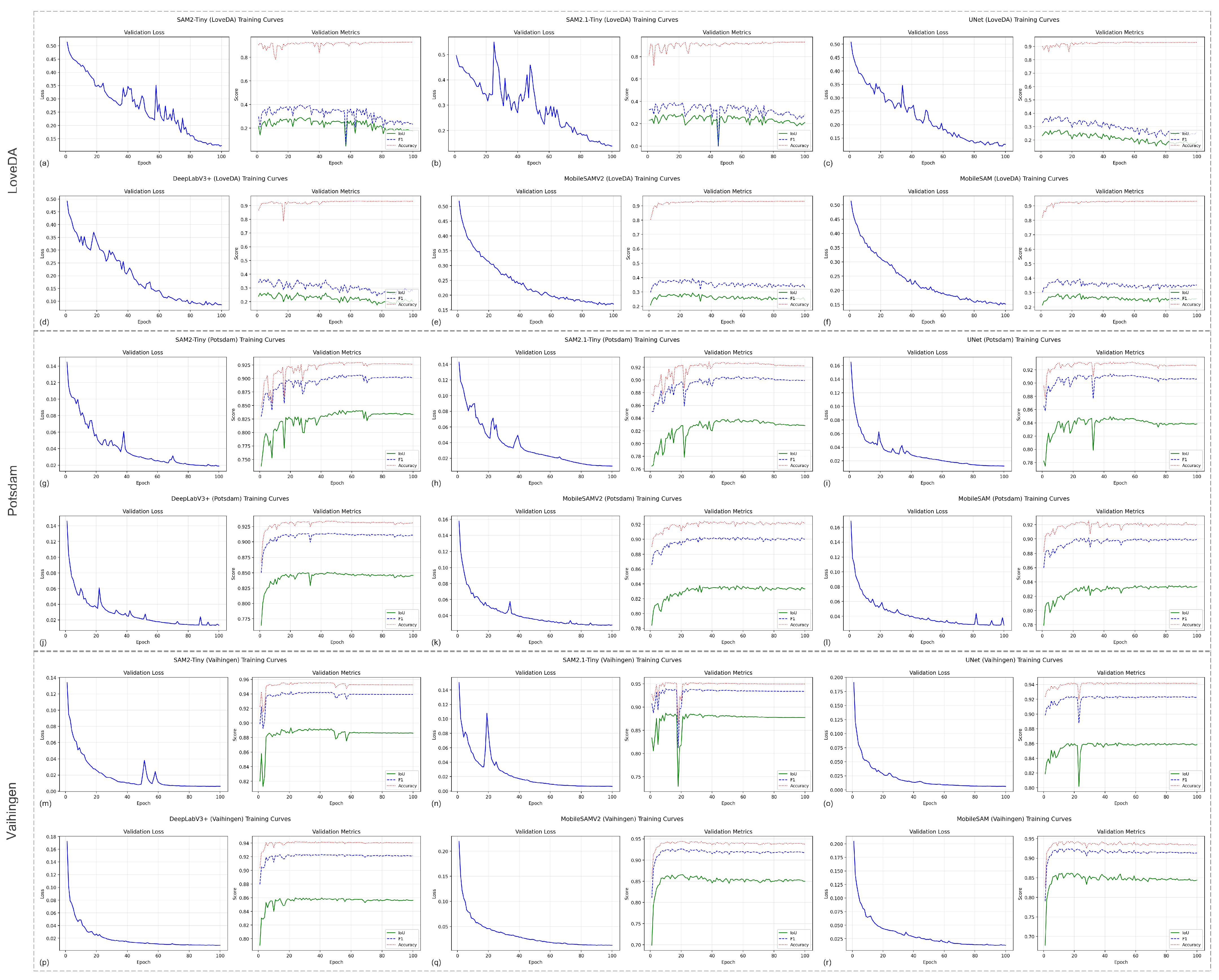
Under the unified experimental protocol described above, the eight models were trained and evaluated using the same training, validation, and test splits.

Table 4. Comprehensive performance indicator comparison of various deep learning backbone models under unified test set.

Model	mIoU	F1 Score	Acc (%)	Best Epoch
SAM2.1-Tiny	0.7821	0.8688	88.70	3
SAM2-Tiny	0.7780	0.8660	88.33	6
MobileSAMV2	0.7382	0.8316	87.28	16
MobileSAM	0.7369	0.8322	85.95	4
DeepLabV3+	0.7345	0.8360	84.73	5
UNet	0.7157	0.8239	83.48	10
SegEarth-OV	0.3079	0.4205	48.50	—
YOLO11s-seg	0.0670	—	—	—

summarizes the final performance of each model on the Zijinshan test set, and Figure 5 shows the convergence characteristics of the training curves. Together, these results provide the main basis for comparing accuracy, boundary coherence, convergence stability, and inference cost under small-sample conditions.

Table 4 shows a clear performance hierarchy under the unified Zijinshan test protocol. SAM2.1-Tiny and SAM2-Tiny form the first tier, with only a small gap between them, indicating that both models can maintain high-quality vegetation boundaries under small-sample remote sensing conditions. MobileSAMV2 and MobileSAM form the second tier, suggesting that lightweight distilled structures still retain useful spatial priors with limited accuracy loss. DeepLabV3+ and UNet remain practical supervised baselines, but their performance is more constrained by small-sample training and cross-temporal appearance variation. SegEarth-OV and YOLO11s-seg perform substantially lower in this setting, indicating that open-vocabulary segmentation and instance-level representation are less suitable for continuous pixel-level vegetation extraction.

The novelty of this comparison does not lie in reporting a single best mIoU value, but in identifying how different SAM-derived foundation-model variants behave under the same small-sample high-resolution vegetation segmentation protocol. In particular, the SAM2/SAM2.1 variants indicate the accuracy and convergence advantage of stronger foundation backbones, whereas MobileSAM/MobileSAMV2 reveal the cost of lightweight compression and the corresponding accuracy–efficiency trade-off. Therefore, Table 4 serves as the quantitative basis for the subsequent analyses of computational cost, cross-domain robustness, visual boundary quality, and CT-PLST self-training.

Figure 5 further summarizes the convergence behavior. SAM2.1-Tiny reaches its best checkpoint at epoch 3 with an mIoU of 0.7821 and SAM2-Tiny peaks at epoch 6 with an mIoU of 0.7780, indicating early stabilization and high final accuracy. MobileSAM and DeepLabV3+ also peak early, whereas MobileSAMV2 and UNet require longer training to reach their best checkpoints. Overall, the foundation-model family achieves the highest scores with relatively stable validation curves, while the classic supervised baselines show greater dependence on the limited training samples and data split.

3.2.2. Computational Cost and Inference Efficiency

Accuracy alone is insufficient for model selection in practical remote sensing workflows, because large-area vegetation mapping also depends on inference latency, memory footprint, and hardware cost. Therefore, the number of parameters, floating-point operations (FLOPs), single-image inference time, frames per second (FPS), and peak GPU memory were measured under a unified benchmark protocol. Dense segmentation models were tested with one forward pass after warm-up, while prompt-based models were timed with fixed prompt-to-box inference settings.

The fastest dense baselines in

Table 5. Computational-cost comparison of the evaluated models.

Model	Params (M)	FLOPs (G)	Time (ms/img)	FPS	Memory (MB)	Input
SAM2-Tiny	28.179	213.325	11.455	87.30	501.4	1024 × 1024
SAM2.1-Tiny	28.179	213.769	11.414	87.61	503.3	1024 × 1024
MobileSAM	7.025	81.399	6.534	153.04	278.5	1024 × 1024
MobileSAMV2	7.025	81.399	6.552	152.62	278.5	1024 × 1024
UNet	24.437	24.560	2.399	416.79	154.0	320 × 320
DeepLabV3+	26.678	73.822	2.970	336.66	242.3	512 × 512
YOLO11s-seg	10.083	22.779	5.251	190.44	97.4	512 × 512
SegEarth-OV	149.914	211.451	36.195	27.63	3531.7	448 × 448
DINOv2 ViT-L/14-Reg	304.931	833.594	7.076	141.32	1237.6	518 × 518
DINOv3 ViT-L/16	303.715	469.286	10.530	94.97	1225.6	512 × 512
QwenVL2.5-3B	3754.623	4366.981	772.743	1.29	7331.9	512 × 512
LocateAnything-3B	3517.975	7904.232	732.411	1.37	7874.6	512 × 512

are UNet and DeepLabV3+, which reach 416.79 FPS and 336.66 FPS, respectively. YOLO11s-seg has the smallest memory footprint among the evaluated dense or instance-segmentation models, while MobileSAM and MobileSAMV2 provide a favorable balance between parameter count and inference speed. SAM2-Tiny and SAM2.1-Tiny require higher FLOPs than the lightweight SAM variants but remain within a practical latency range. SegEarth-OV has the highest memory footprint among the original comparison models because of its CLIP-based backbone and feature upsampling module. The DINO-based supplements have substantially larger parameter counts but still maintain usable forward latency on the tested hardware. QwenVL2.5-3B and LocateAnything-3B are much more expensive because their inference involves prompt-conditioned generation or grounding; their FLOPs are therefore best interpreted as prompt-inference estimates rather than as directly equivalent dense segmentation forward-pass costs.

3.2.3. Visual Results of Typical Samples and Local Boundary Performance

While Tables and Figures above explain who is better overall, this section answers why it is better. The real difficulty of vegetation segmentation tasks often lies not in large green spaces themselves but in edge areas where vegetation intersects with shadows, buildings, roads, and bare land. Therefore, representative visual examples from LoveDA, Zijinshan, Potsdam, and Vaihingen are used to compare local boundary continuity, false positives around non-vegetation objects, and missed vegetation regions under different image distributions.

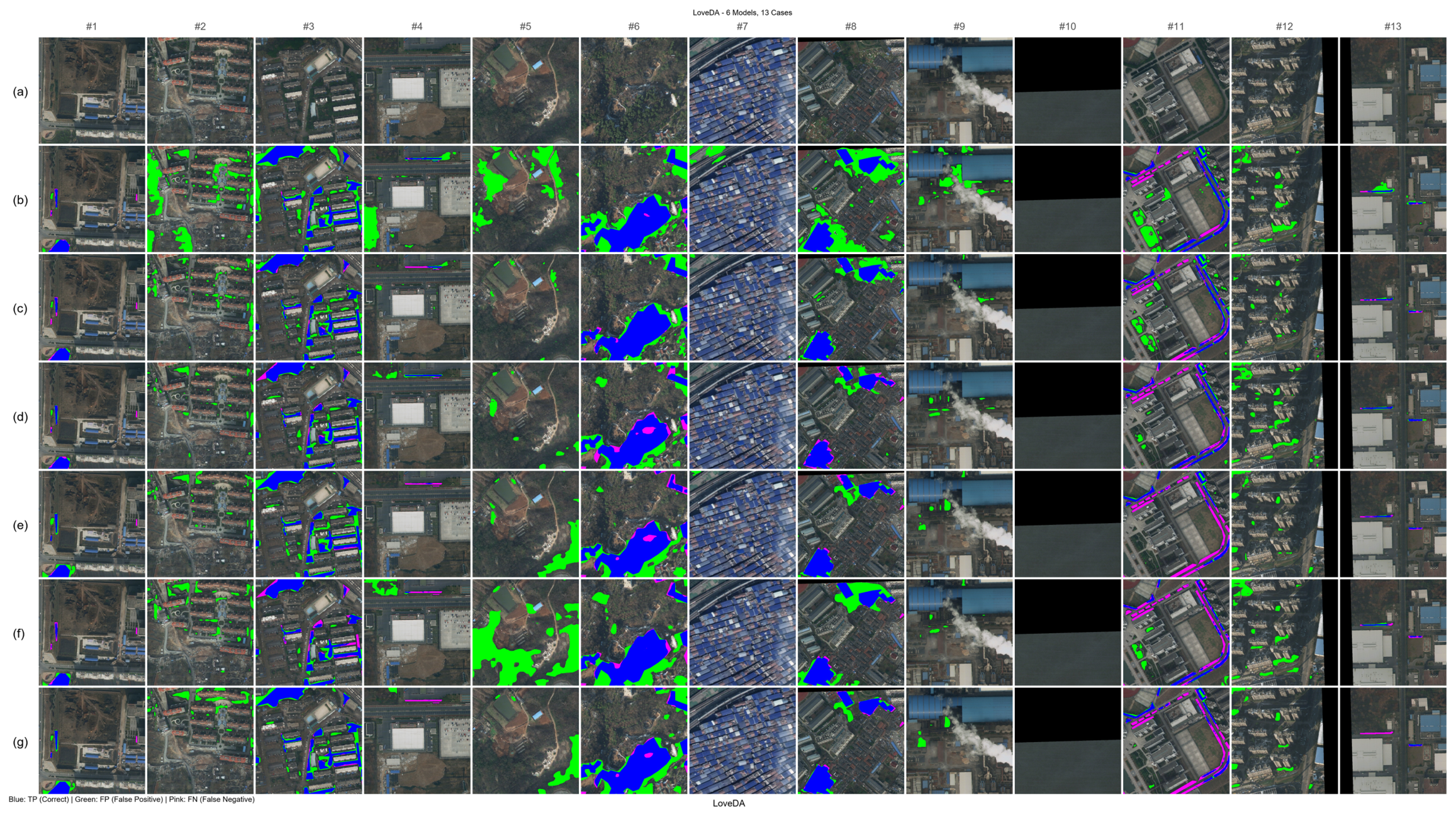
In Figure 6, the displayed model rows are ordered as follows: (b) UNet, (c) DeepLabV3+, (d) SAM2-Tiny, (e) MobileSAM, (f) SAM2.1-Tiny, and (g) MobileSAMV2. The differences mainly appear around fragmented vegetation patches and shadowed urban boundaries rather than in large homogeneous green regions. For example, in cases #3 and #11, UNet and DeepLabV3+ contain more green false-positive responses along roofs, roads, and shadowed surfaces, whereas SAM2-Tiny and SAM2.1-Tiny keep the vegetation masks more confined to the true vegetation regions. In cases #5 and #6, the two lightweight SAM variants retain the main vegetation bodies, but their differences are visually subtle at this display scale; the more evident contrast in these examples is between the SAM-derived rows and the classical supervised baselines, especially in local fragmentation and missed thin vegetation strips.

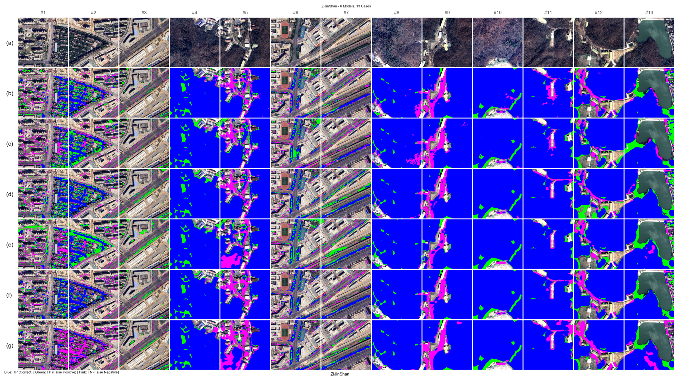
Figure 7 uses the same row order as Figure 6. In the same-domain high-resolution setting, SAM2-Tiny in row (d) and SAM2.1-Tiny in row (f) produce coherent masks along forest margins and lake-side vegetation, which is consistent with their top mIoU scores in Table 4. In case #2, the classical supervised baselines show more scattered green false positives and pink false negatives around roads, roofs, and vegetation–building transitions, while the SAM2 variants retain larger continuous blue true-positive regions. In case #12, MobileSAMV2 in row (g) follows the SAM2 variants more closely than MobileSAM in row (e), especially near lake-side and forest-margin boundaries where small discontinuities are more visible in the lightweight MobileSAM output.

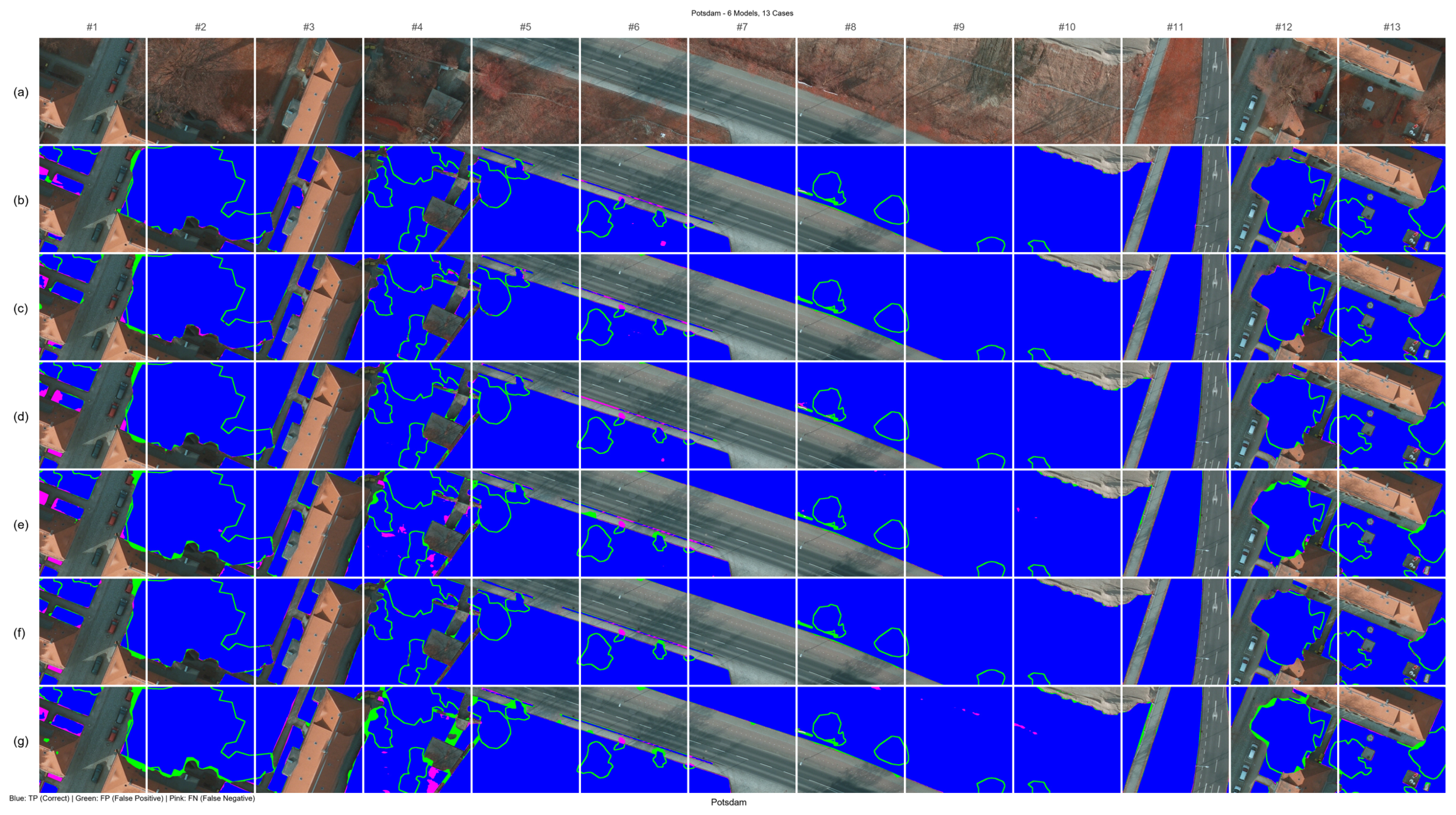
In Figure 8, the urban structure is more regular and the vegetation boundaries are sharper, so the six displayed models appear very close in most large vegetation regions. This visual similarity is consistent with the Potsdam results in

Table 6. Cross-domain mIoU comparison of various models on public remote sensing datasets.

Model	LoveDA	Potsdam	Vaihingen	Average
SAM2-Tiny	0.2906	0.8410	0.8933	0.6750
SAM2.1-Tiny	0.2889	0.8387	0.8868	0.6715
MobileSAM	0.2924	0.8348	0.8620	0.6631
MobileSAMV2	0.2934	0.8377	0.8656	0.6656
UNet	0.2738	0.8494	0.8611	0.6614
DeepLabV3+	0.2650	0.8506	0.8598	0.6585
YOLO11s-seg	0.2460	0.5775	0.7663	0.5299
SegEarth-OV	0.0401	0.1820	0.4450	0.2224

, where DeepLabV3+ and UNet obtain the highest mIoU values and the SAM-derived models remain only slightly lower. Therefore, Figure 8 is mainly used to show that all six displayed models can recover the dominant regular green-space patterns under this ultra-high-resolution urban setting. The remaining differences are subtle and are mostly limited to small tree crowns, narrow roadside vegetation, and vegetation–road or vegetation–building contact zones, where minor boundary smoothing, local false positives, or small missed patches can appear depending on the model.

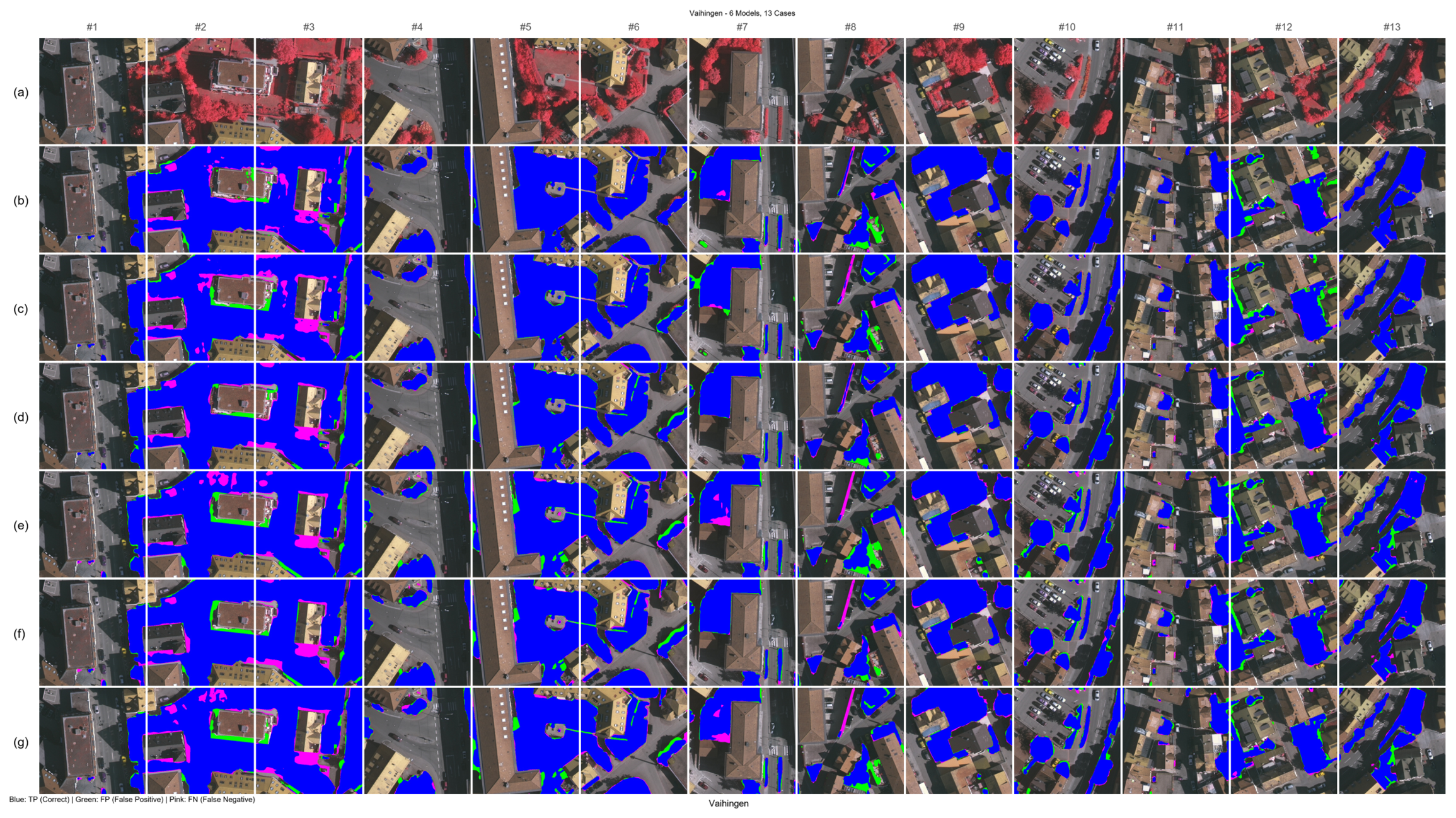
Figure 9 presents the Vaihingen results under dense urban shadows, narrow urban structures, and mixed tree canopies. In many columns, the six displayed models produce visually similar masks for large vegetation regions, so the figure should be interpreted together with the quantitative results in Table 6. The visible differences are mostly local, including small pink false-negative fragments near tree-canopy edges, green false-positive responses around roofs or shadowed surfaces, and slight changes in the continuity of narrow vegetation strips. In cases #10–#13, UNet and DeepLabV3+ in rows (b) and (c) remain acceptable for large regular vegetation areas, but their outputs show more local instability near roof–shadow transitions and narrow vegetation strips. Taken together, Figure 6, Figure 7, Figure 8 and Figure 9 show that the visual comparison is most informative in boundary and transition regions, whereas large homogeneous vegetation blocks often appear similar across models.

3.2.4. Cross-Dataset Generalization and Robustness Results

If only looking at results on one Zijinshan dataset, we cannot explain the true generalization capability of models. Therefore, this study further transfers trained models to three public datasets—LoveDA, Potsdam, and Vaihingen—for comparison. The goal here is not to prove that a certain model performs well on a certain dataset by chance but to test whether it can maintain stability under different sensors, different urban structures, and different resolution conditions.

Table 6 shows that model transfer differs substantially across the three public datasets. LoveDA is the hardest setting: the best score is 0.2934, and the top four models are tightly clustered within 0.2889–0.2934. By contrast, Potsdam and Vaihingen produce much higher top-tier scores. On Potsdam, DeepLabV3+ and UNet obtain the highest mIoU values, indicating that classic supervised dense segmentation remains highly effective in regular ultra-high-resolution urban scenes. On Vaihingen, SAM2-Tiny and SAM2.1-Tiny show the strongest transfer performance, suggesting better robustness under dense shadows and narrow urban structures. YOLO11s-seg and SegEarth-OV remain lower overall, suggesting that instance-level and open-vocabulary paradigms are less suitable for pixel-accurate vegetation extraction in this setting.

The cross-dataset mIoU values should also be interpreted with caution because transfer performance is affected by sensor and geographic domains, acquisition conditions, annotation style, and spatial resolution. For example, Zijinshan is collected at 0.75 m resolution, whereas LoveDA is 0.3 m. The resolution gap changes the apparent size of vegetation crowns, roads, shadows, boundary complexity, and mixed-pixel proportions. Therefore, the low LoveDA mIoU values are best understood as the combined effect of domain shift and resolution mismatch, not as evidence that the models completely fail to generalize. In this study, the cross-dataset results are used as robustness evidence under realistic remote sensing transfer conditions rather than as an absolute dataset-independent ranking. A dedicated resolution-adaptation ablation would be required to isolate the pure effect of scale difference.

3.2.5. Observation-Condition Robustness

Cross-dataset testing mainly reflects domain and resolution shifts, whereas practical remote sensing inference also faces acquisition-condition changes within the same region. To evaluate this aspect, an inference-only perturbation test was conducted on Zijinshan test imagery by applying brightness variation, contrast variation, Gaussian blur, and synthetic shadow/illumination changes to the input images while keeping the ground-truth masks and model weights unchanged.

Table 7. Reference accuracy and observation-condition robustness comparison on Zijinshan test imagery.

Model	n	Ref. mIoU	Mean ΔmIoU	Worst ΔmIoU	Worst Condition
SAM2-Tiny	32	0.7780	−0.0017	−0.0122	Gaussian blur k7
SAM2.1-Tiny	32	0.7821	−0.0026	−0.0207	Gaussian blur k7
MobileSAM	32	0.7369	−0.0032	−0.0352	Gaussian blur k7
MobileSAMV2	32	0.7382	−0.0013	−0.0303	Gaussian blur k7
UNet	32	0.7157	−0.0113	−0.1023	Brightness 1.30
DeepLabV3+	32	0.7345	−0.0384	−0.2416	Gaussian blur k7
YOLO11s-seg	32	0.0670	−0.0074	−0.0573	Gaussian blur k7
SegEarth-OV	32	0.3079	+0.0084	−0.0291	Shadow strong
DINOv2 ViT-L/14-Reg	67	0.7466	−0.0004	−0.0022	Gaussian blur k7
DINOv3 ViT-L/16	67	0.7683	−0.0004	−0.0167	Brightness 0.70
QwenVL2.5-3B	67	0.6212	−0.0096	−0.0332	Brightness 1.30
LocateAnything-3B	67	0.5747	+0.0019	−0.0373	Contrast 1.10

summarizes the reference Zijinshan mIoU from the main and supplementary evaluations, the average mIoU change over all perturbation settings, and the worst-case mIoU change for the original comparison models and the supplementary foundation or prompt-based models. The reference mIoU values provide consistency with the main quantitative tables, whereas the perturbation deltas describe each model’s relative sensitivity to acquisition-condition changes.

The perturbation results show that the SAM-family dense segmentation models remain stable under moderate brightness, contrast, and shadow changes, while Gaussian blur is the most damaging condition for most original comparison models. SAM2.1-Tiny and SAM2-Tiny retain the strongest reference mIoU among the original comparison models and show only small average degradation under perturbations. MobileSAMV2 has the smallest mean degradation among the original models, although its worst case still occurs under strong blur. DeepLabV3+ is the most sensitive to blur, indicating that local texture smoothing can strongly affect its boundary recovery. Among the supplementary models, DINOv2 and DINOv3 show very small average mIoU changes, suggesting strong stability of their frozen visual representations under the tested acquisition-condition changes. QwenVL2.5-3B and LocateAnything-3B are less directly comparable to dense segmentation models because their outputs are converted from prompt-based boxes to coarse masks, but their perturbation deltas indicate that prompt-conditioned localization remains sensitive to changes that alter object saliency or contrast.

3.2.6. Supplementary Evaluation of Recent Foundation- and Prompt-Based Models

To further examine whether newer foundation models change the conclusions above, this study additionally evaluated DINOv2, DINOv3, QwenVL2.5-3B, and LocateAnything-3B on the same four-dataset setting. Because these models do not share the same task formulation, the results are interpreted by task type. DINOv2 and DINOv3 are dense segmentation supplements with frozen visual backbones and trained segmentation heads, whereas QwenVL2.5-3B and LocateAnything-3B are prompt-based localization or grounding supplements whose predicted boxes are converted into coarse masks for approximate comparison.

Table 8. Supplementary cross-dataset mIoU comparison of recent foundation- and prompt-based models.

Model	Zijinshan	LoveDA	Potsdam	Vaihingen	Average
DINOv2 ViT-L/14-Reg	0.7466	0.7076	0.8403	0.8782	0.7932
DINOv3 ViT-L/16	0.7683	0.7505	0.8530	0.8793	0.8128
QwenVL2.5-3B	0.6212	0.1175	0.3482	0.4615	0.3871
LocateAnything-3B	0.5747	0.1122	0.5038	0.5444	0.4338

summarizes the supplementary model results in the same dataset-by-dataset layout as the cross-domain comparison above. The DINO-based dense segmentation supplements perform strongly across all four datasets. DINOv3 obtains the higher average mIoU (0.8128) than DINOv2 (0.7932), with the clearest gains on Zijinshan and LoveDA. The LoveDA result is especially informative because DINOv3 reaches 0.7505 mIoU under the four-dataset training protocol, indicating that stronger pretrained visual representations can reduce the difficulty caused by mixed urban–rural backgrounds and scale variation. QwenVL2.5-3B and LocateAnything-3B provide useful vegetation localization cues, but their coarse mask outputs cannot recover fine vegetation boundaries in the same way as dense segmentation models. Both prompt-based models perform weakly on LoveDA, where heterogeneous land-cover composition and fragmented vegetation regions make box-level localization insufficient for pixel-accurate vegetation extraction. These results indicate that prompt-based vision–language and grounding models are useful as auxiliary localization tools, but task-specific dense segmentation remains necessary for accurate high-resolution vegetation mapping.

3.2.7. CT-PLST Self-Training and Threshold Ablation Results

In the final part of the results section, we need to answer a more methodological question: When manual annotations are extremely scarce, can models continue to gain improvements through unlabeled temporal data? To verify this, this study adopts the CT-PLST self-training strategy and conducts ablation analysis on threshold sensitivity.

The self-training results in

Table 9. Model gain comparison before and after self-training.

Model	Initial mIoU	After Self-Training	Improvement	Relative Gain
SAM2-Tiny	0.7776	0.7888	+0.0112	+1.44%
UNet	0.7415	0.7667	+0.0252	+3.40%

show that CT-PLST improves both SAM2-Tiny and UNet, although the improvement pattern differs. SAM2-Tiny gains a modest but consistent margin because its initial performance is already high, whereas UNet improves more clearly when additional pseudo-labeled supervision is introduced. This indicates that self-training can compensate for limited manual annotation, but its effect still depends on pseudo-label reliability.

The confidence-threshold ablation further shows that $\tau =0.70$ provides the best trade-off in this experiment. At this setting, CT-PLST keeps 67 pseudo-labeled samples and reaches mIoU 0.7888, F1 0.8745, and Acc 0.8877. Raising the threshold to 0.75 or 0.80 keeps the same number of samples but slightly lowers mIoU to 0.7859 and 0.7858, while $\tau =0.85$ reduces the retained set to 66 samples and still does not improve IoU. Thus, the selected threshold is supported by a measurable, although small, advantage over the stricter settings. This analysis is related to, but different from, multi-threshold image binarization in remote sensing: multi-threshold methods usually divide spectral-index or intensity distributions into several land-cover intervals, whereas the present threshold controls whether a model prediction is reliable enough to enter the pseudo-labeled training set. The selected $\tau =0.70$ therefore reflects a trade-off between data quality and the possibility for self-training rather than a direct vegetation/non-vegetation spectral threshold.

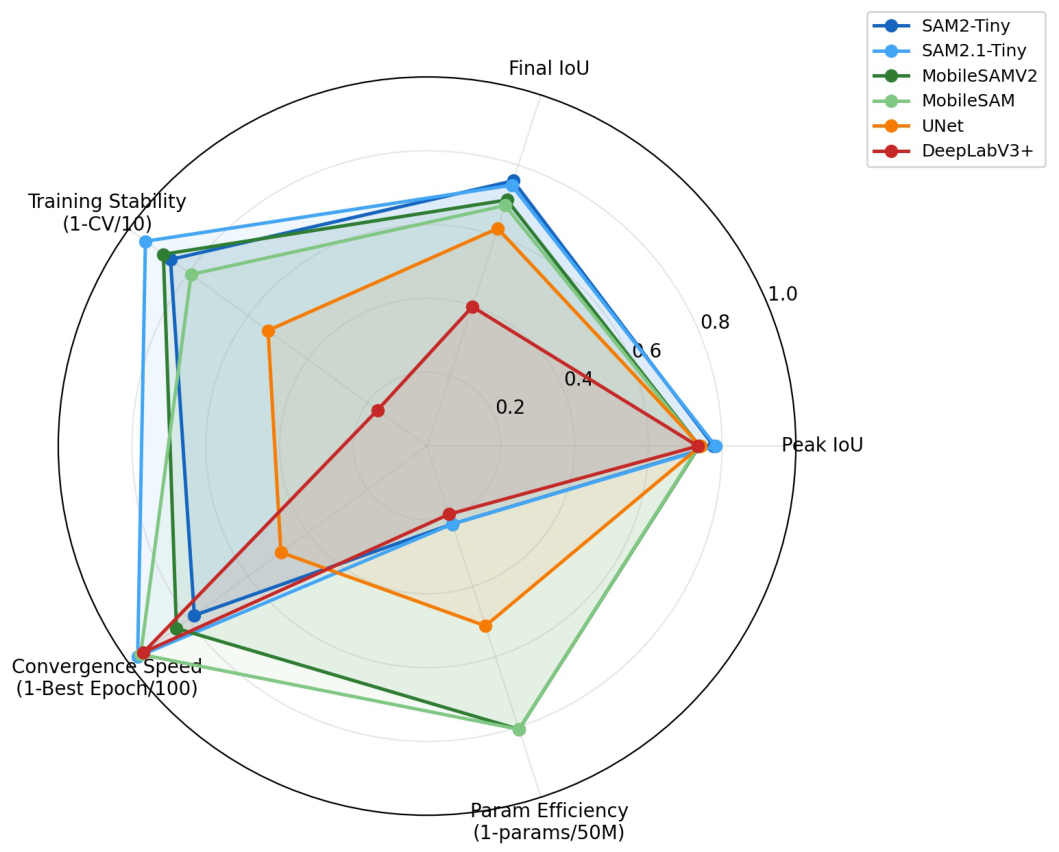
The radar chart in Figure 10 summarizes the overall trade-off more directly. SAM2.1-Tiny is the most balanced in terms of accuracy and stability, but its deployment cost is still higher than that of MobileSAM series. MobileSAMV2 and MobileSAM are more suitable for rapid processing and edge-oriented scenarios because of their higher efficiency, although their accuracy is slightly lower than the SAM2 series. UNet and DeepLabV3+ remain practical baseline choices when training simplicity and implementation maturity are more important, while YOLO11s-seg and SegEarth-OV are better interpreted as task-specific tools rather than replacements for continuous vegetation segmentation. This also shows that model selection should be guided by the full set of performance constraints rather than by a single score.

From a practical perspective, this paper still has three limitations. First, the SAM series provide high accuracy, but their inference cost and memory footprint remain higher than those of conventional convolutional baselines, which limits direct deployment on extremely resource-constrained devices. Second, CT-PLST depends on pseudo-label quality, so its benefit will drop when the scene is severely noisy, the boundaries are extremely fragmented, or the temporal gap is too large. Third, the current data sources mainly cover one region and a small number of public datasets, so the adaptation ability under extreme seasonal change, multi-spectral input, and more complex agricultural patterns still needs further verification.

An additional limitation is that the cross-dataset comparison couples domain shift with large resolution differences, especially for LoveDA. Without a controlled resampling experiment, the current results should be viewed as an overall robustness assessment rather than a resolution-normalized generalization study. Future work should therefore add a downsampled LoveDA ablation or a matched-resolution transfer protocol to separate scale effects from semantic transfer effects.

Future work can therefore proceed in three directions: introducing more explicit temporal self-supervision or semi-supervised constraints to stabilize pseudo-label generation; exploring multi-spectral or multimodal fusion to reduce ambiguity caused by shadows and mixed pixels; and building a lighter deployment chain so that SAM-based models can be used more efficiently in mobile, edge, or large-scale rapid inspection scenarios.

4. Discussion

Based on the experimental results in the previous section, this section further analyzes the deep mechanisms of different models’ performance in small-sample remote sensing vegetation segmentation tasks from the perspective of understanding why such results are obtained, systematically revealing the internal determining factors of performance differences. Unlike simply listing numerical values, this section focuses more on the coupling relationship between model structure, training methods, cross-domain migration capabilities, and deployment constraints, discovering the design logic and application boundaries of different technical paradigms through comparative analysis.

The results show that SAM2 series models achieved better performance in final IoU and F1 scores, while MobileSAM series have more advantages in speed and resource occupation. DeepLabV3+ and UNet, as classic fully supervised models, can still output stable results but are easily affected by local texture bias in complex boundaries and cross-temporal scenarios. YOLO11s-seg and SegEarth-OV, respectively, reflect the boundaries of instance segmentation paradigm and open-vocabulary paradigm in continuous semantic segmentation problems.

The more important methodological point is that CT-PLST should not be interpreted as a completely new self-training family, but as a task-specific adaptation of classical pseudo-label learning to cross-temporal remote sensing data. In Lee’s pseudo-label framework, unlabeled samples are assigned hard labels by the current model and then folded back into supervised learning [31]; CT-PLST follows this hard-label idea, but the novelty lies in using temporally separated imagery from the same region as a structured source of unlabeled data, so the additional supervision comes from seasonal appearance change rather than from merely expanding the sample count. Noisy Student also uses teacher-generated pseudo-labels, but it emphasizes repeated teacher–student iteration together with injected noise and large-scale data augmentation on largely in-distribution samples [34]. In contrast, CT-PLST keeps the teacher stage explicitly tied to the best validation checkpoint, filters pseudo-labels by a confidence threshold, and then re-trains on cross-temporal imagery to confront seasonal drift, brightness change, and boundary perturbation. FixMatch is even closer in spirit to consistency regularization: it couples weak and strong augmentations of the same image and enforces agreement under confidence filtering [32]. CT-PLST does not optimize a weak/strong augmentation consistency objective; instead, it transfers high-confidence predictions across time, so the supervisory signal is temporal consistency rather than augmentation consistency. Therefore, the core contribution of CT-PLST is not a new loss form, but a more suitable data construction strategy for remote sensing scenes where unlabeled images naturally arrive as time series.

This also matters for the cross-dataset discussion, because the same model can look strong on one domain yet weak on another when spatial resolution changes. In that sense, CT-PLST demonstrates how to exploit temporal structure, but the cross-dataset section shows that resolution remains an independent axis of robustness that is not solved by pseudo-labeling alone.

This distinction also explains why the gain is modest rather than dramatic. Self-training methods usually produce the largest gains when the baseline is weak or when the unlabeled data distribution is very rich but the pseudo-label quality remains controllable. Here, SAM2-Tiny already starts from a strong foundation-model prior, so there is less headroom for absolute mIoU growth. The observed +1.44% gain is therefore better understood as a robustness-oriented improvement: it comes from reduced missed boundaries, more stable masks under temporal shift, and better exploitation of unlabeled imagery, not from a wholesale redesign of the segmentation pipeline. In this sense, the value of CT-PLST is that it converts the temporal dimension itself into a supervision source, which is particularly appropriate for remote sensing scenarios where appearance changes are driven by season, illumination, and acquisition date rather than by random augmentation alone.

5. Conclusions

This paper focuses on the small-sample vegetation segmentation problem in high-resolution remote sensing imagery. Combined with Zijinshan’s own multi-temporal data and public datasets such as LoveDA, Potsdam, and Vaihingen, it systematically compares eight representative models, including SAM2-Tiny, SAM2.1-Tiny, MobileSAM, MobileSAMV2, UNet, DeepLabV3+, YOLO11s-seg, and SegEarth-OV, within a unified experimental framework under small-sample conditions, clarifying the performance boundaries and application limitations of foundation models, traditional convolutional networks, open-vocabulary models, and instance segmentation models in vegetation segmentation tasks. Through systematic comparison, it clearly indicates the outstanding advantages of vision foundation models in small-sample remote sensing tasks and further analyzes the improvement effect of the cross-temporal pseudo-label self-training strategy CT-PLST on model generalization capabilities.

Experimental results show that under conditions of complex vegetation boundaries, significant shadow interference, high scene structure mixing degree, and extremely few annotation samples, foundation models can obtain optimal segmentation quality and the most stable boundary recovery capability after reasonable fine-tuning. Among them, SAM2.1-Tiny achieved the highest mIoU (0.7821) on the Zijinshan dataset, a 5.5% improvement over traditional U-Net; SAM2-Tiny further improved to 0.7888 (+1.44%) after CT-PLST self-training, fully verifying the effective supplementary role of high-confidence pseudo-labels on few-shot supervision signals; MobileSAMV2 and MobileSAM significantly improved inference efficiency while maintaining high accuracy, making them more suitable for resource-constrained scenarios. In comparison, UNet and DeepLabV3+ still have strong usability but are relatively limited in cross-domain generalization and fine-grained boundary expression; YOLO11s-seg and SegEarth-OV have advantages in their respective paradigms but are not suitable for directly replacing vegetation segmentation tasks oriented toward continuous semantic regions.

Overall, the core research insight of this paper is as follows. The key to small-sample remote sensing vegetation segmentation lies in systematic model evaluation and scientific selection judgment, rather than blindly pursuing the largest model scale. By establishing an organic closed loop of strong prior foundation models and high-quality pseudo-label self-training, feature distribution can be continuously improved and noise propagation suppressed under annotation-scarce conditions. The success of CT-PLST further proves that in remote sensing monitoring with abundant multi-temporal data, fully activating unlabeled temporal information is an effective way to break through small-sample bottlenecks. At the same time, this paper also has certain limitations, such as data sources and geomorphological conditions still insufficient to cover all extreme scenarios, pseudo-label filtering and error propagation mechanisms still have further optimization space, and the training and inference costs of foundation models also require continued compression in extremely resource-constrained environments. Future work can continue to deepen research in four directions—temporal information fusion, combination of self-supervision and semi-supervision, introduction of multi-spectral information, and construction of lightweight deployment chains—so that models can better serve practical tasks such as ecological surveys, forestry monitoring, urban green space assessment, and land use change analysis.

References

1. Moghimi, A.; Welzel, M.; Celik, T.; Schlurmann, T. A Comparative Performance Analysis of Popular Deep Learning Models and Segment Anything Model (SAM) for River Water Segmentation in Close-Range Remote Sensing Imagery. IEEE Access 2024, 12, 52067–52085. [Google Scholar] [CrossRef] [Scilit]
2. Ronneberger, O.; Fischer, P.; Brox, T. U-Net: Convolutional Networks for Biomedical Image Segmentation. In Proceedings of the Medical Image Computing and Computer-Assisted Intervention MICCAI, Munich, Germany, 5–9 October 2015. [Google Scholar]
3. Long, J.; Shelhamer, E.; Darrell, T. Fully Convolutional Networks for Semantic Segmentation. In Proceedings of the IEEE Conference on Computer Vision and Pattern Recognition CVPR, Boston, MA, USA, 7–12 June 2015. [Google Scholar]
4. He, K.; Zhang, X.; Ren, S.; Sun, J. Deep Residual Learning for Image Recognition. In Proceedings of the IEEE Conference on Computer Vision and Pattern Recognition CVPR, Las Vegas, NV, USA, 27–30 June 2016. [Google Scholar]
5. Ioffe, S.; Szegedy, C. Batch Normalization: Accelerating Deep Network Training by Reducing Internal Covariate Shift. In Proceedings of the 32nd International Conference on Machine Learning (ICML), Lille, France, 6–11 July 2015. [Google Scholar]
6. Kingma, D.P.; Ba, J. Adam: A Method for Stochastic Optimization. In Proceedings of the International Conference on Learning Representations ICLR, San Diego, CA, USA, 7–9 May 2015. [Google Scholar]
7. Chen, L.C.; Papandreou, G.; Kokkinos, I.; Murphy, K.; Yuille, A.L. DeepLab: Semantic Image Segmentation with Deep Convolutional Nets, Atrous Convolution, and Fully Connected CRFs. IEEE Trans. Pattern Anal. Mach. Intell. 2018, 40, 834–848. [Google Scholar] [CrossRef] [Scilit] [PubMed]
8. Chen, L.C.; Zhu, Y.; Papandreou, G.; Schroff, F.; Adam, H. Encoder-Decoder with Atrous Separable Convolution for Semantic Image Segmentation. In Proceedings of the European Conference on Computer Vision ECCV, Munich, Germany, 8–14 September 2018. [Google Scholar]
9. Zhao, H.; Shi, J.; Qi, X.; Wang, X.; Jia, J. Pyramid Scene Parsing Network. In Proceedings of the IEEE Conference on Computer Vision and Pattern Recognition CVPR, Honolulu, HI, USA, 21–26 July 2017. [Google Scholar]
10. Lin, T.Y.; Dollár, P.; Girshick, R.; He, K.; Hariharan, B.; Belongie, S. Feature Pyramid Networks for Object Detection. In Proceedings of the IEEE Conference on Computer Vision and Pattern Recognition CVPR, Honolulu, HI, USA, 21–26 July 2017. [Google Scholar]
11. Dosovitskiy, A.; Beyer, L.; Kolesnikov, A.; Weissenborn, D.; Zhai, X.; Unterthiner, T.; Dehghani, M.; Minderer, M.; Heigold, G.; Gelly, S.; et al. An Image Is Worth 16x16 Words: Transformers for Image Recognition at Scale. In Proceedings of the International Conference on Learning Representations ICLR, Virtual, 3–7 May 2021. [Google Scholar]
12. Liu, Z.; Lin, Y.; Cao, Y.; Hu, H.; Wei, Y.; Zhang, Z.; Lin, S.; Guo, B. Swin Transformer: Hierarchical Vision Transformer using Shifted Windows. In Proceedings of the IEEE/CVF International Conference on Computer Vision ICCV, Montreal, QC, Canada, 10–17 October 2021. [Google Scholar]
13. Kirillov, A.; Mintun, E.; Ravi, N.; Mao, H.; Rolland, C.; Gustafson, L.; Xiao, T.; Whitehead, S.; Berg, A.C.; Lo, W.Y.; et al. Segment Anything. In Proceedings of the IEEE/CVF International Conference on Computer Vision ICCV, Paris, France, 1–6 October 2023. [Google Scholar]
14. Ravi, N.; Gabeur, V.; Hu, Y.T.; Hu, R.; Ryali, C.; Ma, T.; Khedr, H.; Rädle, R.; Rolland, C.; Gustafson, L.; et al. SAM 2: Segment Anything in Images and Videos. arXiv 2024, arXiv:2408.00714. [Google Scholar]
15. Zhang, C.; Han, D.; Qiao, Y.; Kim, J.U.; Bae, S.H.; Lee, S.; Hong, C.S. MobileSAM: Exploring SAM in Mobile Scenarios. arXiv 2023, arXiv:2306.14289. [Google Scholar]
16. Zhao, X.; Ding, W.; An, Y.; Du, Y.; Yu, T.; Li, M.; Tang, M.; Wang, J. FastSAM: Fast Segment Anything. arXiv 2023, arXiv:2306.12156. [Google Scholar]
17. Xie, E.; Wang, W.; Yu, Z.; Anandkumar, A.; Alvarez, J.M.; Luo, P. SegFormer: Simple and Efficient Design for Semantic Segmentation with Transformers. In Proceedings of the Advances in Neural Information Processing Systems NeurIPS, Virtual, 6–14 December 2021. [Google Scholar]
18. Guo, M.H.; Lu, C.Z.; Hou, Q.; Liu, Z.N.; Cheng, M.M.; Hu, S.M. SegNeXt: Rethinking Convolutional Attention Design for Semantic Segmentation. In Proceedings of the Advances in Neural Information Processing Systems NeurIPS, New Orleans, LA, USA, 28 November–9 December 2022. [Google Scholar]
19. Cheng, B.; Misra, I.; Schwing, A.G.; Kirillov, A.; Girdhar, R. Mask2Former: Masked-attention Mask Transformer for Universal Image Segmentation. In Proceedings of the IEEE Conference on Computer Vision and Pattern Recognition CVPR, New Orleans, LA, USA, 19–24 June 2022. [Google Scholar]
20. Li, F.; Zhang, H.; Xu, H.; Liu, S.; Zhang, L.; Ni, L.M.; Shum, H.Y. Mask DINO: Towards a Unified Transformer-based Framework for Object Detection and Segmentation. In Proceedings of the IEEE Conference on Computer Vision and Pattern Recognition CVPR, Vancouver, BC, Canada, 18–22 June 2023. [Google Scholar]
21. He, K.; Gkioxari, G.; Dollár, P.; Girshick, R. Mask R-CNN. In Proceedings of the IEEE/CVF International Conference on Computer Vision ICCV, Venice, Italy, 22–29 October 2017. [Google Scholar]
22. Radford, A.; Kim, J.W.; Hallacy, C.; Ramesh, A.; Goh, G.; Agarwal, S.; Sastry, G.; Askell, A.; Mishkin, P.; Clark, J.; et al. Learning Transferable Visual Models From Natural Language Supervision. In Proceedings of the International Conference on Machine Learning ICML, Virtual, 18–24 July 2021. [Google Scholar]
23. Liu, S.; Zeng, Z.; Ren, T.; Li, F.; Zhang, H.; Yang, J.; Jiang, Q.; Li, C.; Yang, J.; Su, H.; et al. Grounding DINO: Marrying DINO with Grounded Pre-Training for Open-Set Object Detection. In European Conference on Computer Vision; Springer: Cham, Switzerland, 2023. [Google Scholar]
24. Wang, C.Y.; Bochkovskiy, A.; Liao, H.Y.M. YOLOv7: Trainable Bag-of-Freebies Sets New State-of-the-Art for Real-Time Object Detectors. arXiv 2022, arXiv:2207.02696. [Google Scholar]
25. Jocher, G.; Chaurasia, A.; Qiu, J. Ultralytics YOLOv8; Ultralytics: Frederick, MD, USA, 2023. [Google Scholar]
26. Rao, Y.; Zhao, W.; Chen, G.; Tang, Y.; Zhu, Z.; Huang, G.; Zhou, J.; Lu, J. DenseCLIP: Language-Guided Dense Prediction with Context-Aware Prompting. In Proceedings of the IEEE Conference on Computer Vision and Pattern Recognition CVPR, New Orleans, LA, USA, 19–24 June 2022. [Google Scholar]
27. Tarvainen, A.; Valpola, H. Mean Teachers Are Better Role Models: Weight-Averaged Consistency Targets Improve Semi-Supervised Deep Learning Results. In Proceedings of the Advances in Neural Information Processing Systems NeurIPS, Long Beach, CA, USA, 4–9 December 2017. [Google Scholar]
28. Broni-Bediako, C.; Xia, J.; Song, J.; Chen, H.; Siam, M.; Yokoya, N. Generalized Few-Shot Semantic Segmentation in Remote Sensing: Challenge and Benchmark. arXiv 2024, arXiv:2406.03463. [Google Scholar]
29. Zhang, H.; He, J.; Chen, S.; Zhan, Y.; Bai, Y.; Qin, Y. Comparing Three Methods of Selecting Training Samples in Supervised Classification of Multispectral Remote Sensing Images. Sensors 2023, 23, 8530. [Google Scholar] [CrossRef] [Scilit] [PubMed]
30. Rusyn, B.; Lutsyk, O.; Kosarevych, R.; Kapshii, O.; Karpin, O.; Maksymyuk, T.; Gazda, J. Rethinking Deep CNN Training: A Novel Approach for Quality-Aware Dataset Optimization. IEEE Access 2024, 12, 137427–137438. [Google Scholar] [CrossRef] [Scilit]
31. Lee, D.H. Pseudo-Label: The Simple and Efficient Semi-Supervised Learning Method for Deep Neural Networks. In Proceedings of the ICML 2013 Workshop on Challenges in Representation Learning (WREPL), Atlanta, GA, USA, 21 June 2013. [Google Scholar]
32. Sohn, K.; Berthelot, D.; Li, C.L.; Zhang, Z.; Carlini, N.; Cubuk, E.D.; Kurakin, A.; Zhang, H.; Raffel, C. FixMatch: Simplifying Semi-Supervised Learning with Consistency and Confidence. In Proceedings of the Advances in Neural Information Processing Systems NeurIPS, Virtual, 6–12 December 2020. [Google Scholar]
33. Berthelot, D.; Carlini, N.; Goodfellow, I.; Papernot, N.; Oliver, A.; Raffel, C. MixMatch: A Holistic Approach to Semi-Supervised Learning. In Proceedings of the Advances in Neural Information Processing Systems NeurIPS, Vancouver, BC, Canada, 8–14 December 2019. [Google Scholar]
34. Xie, Q.; Luong, M.T.; Hovy, E.; Le, Q.V. Self-Training with Noisy Student Improves ImageNet Classification. In Proceedings of the IEEE/CVF Conference on Computer Vision and Pattern Recognition CVPR, Seattle, WA, USA, 13–19 June 2020. [Google Scholar]
35. Hinton, G.; Vinyals, O.; Dean, J. Distilling the Knowledge in a Neural Network. arXiv 2015, arXiv:1503.02531. [Google Scholar]
36. Romero, A.; Ballas, N.; Kahou, S.E.; Chassang, A.; Gatta, C.; Bengio, Y. FitNets: Hints for Thin Deep Nets. In Proceedings of the International Conference on Learning Representations ICLR, San Diego, CA, USA, 7–9 May 2015. [Google Scholar]
37. Park, W.; Kim, D.; Lu, Y.; Cho, M. Relational Knowledge Distillation. In Proceedings of the IEEE Conference on Computer Vision and Pattern Recognition CVPR, Long Beach, CA, USA, 16–20 June 2019. [Google Scholar]
38. Ma, X.; Wu, Q.; Zhao, X.; Zhang, X.; Pun, M.O.; Huang, B. SAM-Assisted Remote Sensing Imagery Semantic Segmentation with Object and Boundary Constraints. arXiv 2023, arXiv:2307.12361. [Google Scholar]
39. Ma, X.; Zhang, X.; Pun, M.O.; Huang, B. MANet: Fine-Tuning Segment Anything Model for Multimodal Remote Sensing Semantic Segmentation. arXiv 2024, arXiv:2403.08992. [Google Scholar]
40. Wang, Y.; Zhang, J.; Jiang, R.; Yang, X.; Yun, T.; Zhang, L. GeoSAM-Lite: A Lightweight Foundation Model for Onboard Remote Sensing Segmentation. arXiv 2026, arXiv:2607.03760. [Google Scholar]
41. Gou, J.; Yu, B.; Maybank, S.J.; Tao, D. Knowledge Distillation: A Survey. Int. J. Comput. Vis. 2021, 129, 1789–1819. [Google Scholar] [CrossRef] [Scilit]
42. Ye, C.; Zhuge, Y.; Zhang, P. Towards Open-Vocabulary Remote Sensing Image Semantic Segmentation. arXiv 2024, arXiv:2405.12779. [Google Scholar]
43. Zhu, X.X.; Tuia, D.; Mou, L.; Xia, G.S.; Zhang, L.; Xu, F.; Fraundorfer, F. Deep Learning in Remote Sensing: A Comprehensive Review and List of Resources. IEEE Geosci. Remote Sens. Mag. 2017, 5, 8–36. [Google Scholar] [CrossRef] [Scilit]
44. Tuia, D.; Persello, C.; Bruzzone, L. Domain Adaptation for the Classification of Remote Sensing Data: A Survey. IEEE Geosci. Remote Sens. Mag. 2016, 4, 41–57. [Google Scholar] [CrossRef] [Scilit]
45. Lu, D.; Weng, Q. A Survey of Image Classification Methods and Techniques for Improving Classification Performance. Int. J. Remote Sens. 2007, 28, 823–870. [Google Scholar] [CrossRef] [Scilit]
46. Camps-Valls, G.; Tuia, D.; Bruzzone, L.; Benediktsson, J.A. Advances in Hyperspectral Image Classification: Earth Observation from the Space Perspective. IEEE Signal Process. Mag. 2014, 31, 45–54. [Google Scholar] [CrossRef] [Scilit]
47. Belgiu, M.; Drăguț, L. Random Forest in Remote Sensing: A Review of Applications and Future Directions. ISPRS J. Photogramm. Remote Sens. 2016, 114, 24–31. [Google Scholar] [CrossRef] [Scilit]
48. Helber, P.; Bischke, B.; Dengel, A.; Borth, D. LoveDA: A Remote Sensing Land-Cover Dataset for Domain Adaptive Semantic Segmentation. ISPRS J. Photogramm. Remote Sens. 2022, 187, 70–84. [Google Scholar]
49. Rottensteiner, F.; Sohn, G.; Jung, J.; Gerke, M.; Baillard, C.; Benitez, S.; Breitkopf, U. The ISPRS Benchmark on Urban Object Classification and 3D Building Reconstruction. ISPRS Ann. 2012, I-3, 293–298. [Google Scholar] [CrossRef] [Scilit]
50. Gerke, M. Use of the STAIR Vision Library Within the ISPRS 2D Semantic Labeling Benchmark (Vaihingen); Technical Report; ITC, University of Twente: Enschede, The Netherlands, 2014. [Google Scholar]
51. International Society for Photogrammetry and Remote Sensing (ISPRS). 2D Semantic Labeling Contest—Potsdam. Available online: https://www.isprs.org/resources/datasets/benchmarks/UrbanSemLab/2d-sem-label-potsdam.aspx (accessed on 21 July 2026).
52. Van Etten, A.; Lindenbaum, D.; Bacastow, T. SpaceNet: A Remote Sensing Dataset and Challenge Series. arXiv 2018, arXiv:1807.01232. [Google Scholar]
53. Neupane, B.; Horanont, T.; Aryal, J. Deep Learning-Based Semantic Segmentation of Urban Features in Satellite Images: A Review and Meta-Analysis. Remote Sens. 2021, 13, 808. [Google Scholar] [CrossRef] [Scilit]
54. Zhang, L.; Zhang, L.; Du, B. Deep Learning for Remote Sensing Data: A Technical Tutorial on the State of the Art. IEEE Geosci. Remote Sens. Mag. 2020, 8, 22–40. [Google Scholar]
55. Mou, L.; Bruzzone, L.; Zhu, X.X. Learning Spectral-Spatial Dependencies for Hyperspectral Image Classification. IEEE Trans. Geosci. Remote Sens. 2017, 55, 5951–5965. [Google Scholar] [CrossRef] [Scilit]
56. Huang, G.; Liu, Z.; Van Der Maaten, L.; Weinberger, K.Q. Densely Connected Convolutional Networks. In Proceedings of the IEEE/CVF Conference on Computer Vision and Pattern Recognition CVPR, Honolulu, HI, USA, 21–26 July 2017. [Google Scholar]
57. Simonyan, K.; Zisserman, A. Very Deep Convolutional Networks for Large-Scale Image Recognition. In Proceedings of the International Conference on Learning Representations ICLR, San Diego, CA, USA, 7–9 May 2015. [Google Scholar]
58. Szegedy, C.; Liu, W.; Jia, Y.; Sermanet, P.; Reed, S.; Anguelov, D.; Erhan, D.; Vanhoucke, V.; Rabinovich, A. Going Deeper with Convolutions. In Proceedings of the IEEE/CVF Conference on Computer Vision and Pattern Recognition CVPR, Boston, MA, USA, 7–12 June 2015. [Google Scholar]
59. Lin, T.Y.; Goyal, P.; Girshick, R.; He, K.; Dollár, P. Focal Loss for Dense Object Detection. In Proceedings of the IEEE/CVF International Conference on Computer Vision ICCV, Lido di Venezia, Venice, Italy, 22–29 October 2017. [Google Scholar]
60. Milletari, F.; Navab, N.; Ahmadi, S.A. V-Net: Fully Convolutional Neural Networks for Volumetric Medical Image Segmentation. In Proceedings of the International Conference on 3D Vision 3DV, Stanford, CA, USA, 25–28 October 2016. [Google Scholar]
61. Sudre, C.H.; Li, W.; Vercauteren, T.; Ourselin, S.; Cardoso, M.J. Generalised Dice Overlap as a Deep Learning Loss Function for Highly Unbalanced Segmentations. In Proceedings of the Deep Learning in Medical Image Analysis (DLMIA 2017), Québec City, QC, Canada, 14 September 2017. [Google Scholar]
62. Jaccard, P. Distribution de la Flore Alpine Dans le Bassin des Dranses et dans Quelques Régions Voisines. Bull. Soc. Vaudoise Sci. Nat. 1901, 37, 241–272. [Google Scholar]
63. Sørensen, T. A Method of Establishing Groups of Equal Amplitude in Plant Sociology Based on Similarity of Species Content. Biol. Skar 1948, 5, 1. [Google Scholar]
64. Dice, L.R. Measures of the Amount of Ecologic Association Between Species. Ecology 1945, 26, 297–302. [Google Scholar] [CrossRef] [Scilit]
65. Cordts, M.; Omran, M.; Ramos, S.; Rehfeld, T.; Enzweiler, M.; Benenson, R.; Franke, U.; Roth, S.; Schiele, B. The Cityscapes Dataset for Semantic Urban Scene Understanding. In Proceedings of the IEEE/CVF Conference on Computer Vision and Pattern Recognition CVPR, Las Vegas, NV, USA, 27–30 June 2016. [Google Scholar]
66. Everingham, M.; Van Gool, L.; Williams, C.K.I.; Winn, J.; Zisserman, A. The PASCAL Visual Object Classes (VOC) Challenge. Int. J. Comput. Vis. 2010, 88, 303–338. [Google Scholar]
67. Audebert, N.; Le Saux, B.; Lefèvre, S. Beyond RGB: Very High Resolution Urban Remote Sensing with Multimodal Deep Networks. ISPRS J. Photogramm. Remote Sens. 2018, 140, 20–32. [Google Scholar] [CrossRef] [Scilit]
68. Oquab, M.; Darcet, T.; Moutakanni, T.; Vo, H.; Szafraniec, M.; Khalidov, V.; Fernandez, P.; Haziza, D.; Massa, F.; El-Nouby, A.; et al. DINOv2: Learning Robust Visual Features without Supervision. arXiv 2023, arXiv:2304.07193. [Google Scholar]
69. Siméoni, O.; Vo, H.V.; Seitzer, M.; Baldassarre, F.; Oquab, M.; Jose, C.; Khalidov, V.; Szafraniec, M.; Yi, S.; Ramamonjisoa, M.; et al. DINOv3. arXiv 2025, arXiv:2508.10104. [Google Scholar]
70. Bai, S.; Chen, K.; Liu, X.; Wang, J.; Ge, W.; Song, S.; Dang, K.; Wang, P.; Wang, S.; Tang, J.; et al. Qwen2.5-VL Technical Report. arXiv 2025, arXiv:2502.13923. [Google Scholar]
71. Wang, Y.; Wang, H.; Shen, Y.; Fei, J.; Li, W.; Jin, G.; Wu, L.; Zhao, R.; Le, X. Semi-Supervised Semantic Segmentation Using Unreliable Pseudo-Labels. In Proceedings of the IEEE/CVF Conference on Computer Vision and Pattern Recognition (CVPR), New Orleans, LA, USA, 19–24 June 2022; pp. 4248–4257. [Google Scholar]
72. Wang, S.; Sun, X.; Hong, D.; Zhou, F. Vision-Language Model Purified Semi-Supervised Semantic Segmentation for Remote Sensing Images. arXiv 2026, arXiv:2605.18974. [Google Scholar]
Figure 1. Comparison of vegetation segmentation methods: (a) original remote sensing imagery of the study area; (b) image threshold segmentation method based on hue–saturation–value (HSV) color space; (c) K-means clustering with morphological post-processing (elliptical kernel 7 × 7); (d) deep-learning-based UNet model (trained on LoveDA dataset). This figure intuitively demonstrates the performance evolution from classic image processing classification to modern deep learning feature extraction in automated vegetation detection.
Remotesensing 18 02487 g001
Figure 2. Small-sample vegetation remote sensing detection evaluation flow based on deep learning containing multi-temporal high spatial resolution data initialization and CT-PLST framework intervention generalization verification structure and analysis system pipeline.
Remotesensing 18 02487 g002
Figure 3. Core innovative method proposed in this paper: Cross-Temporal Pseudo-Label Self-Training (CT-PLST) mechanism workflow. Adaptive threshold cleaning teacher unsupervised feature flow deduction forms student augmentation prior distillation system.
Remotesensing 18 02487 g003
Figure 4. Representative samples from the high-resolution Zijinshan vegetation dataset and surrounding test areas.
Remotesensing 18 02487 g004
Figure 5. Further visualization comparison of training curves to observe whether different models show obvious plateau periods, overfitting, or gradient oscillation in the middle and late stages of training. Panels (af), (gl), and (mr) show the LoveDA, Potsdam, and Vaihingen training curves, respectively; within each dataset, the panels are ordered as SAM2-Tiny, SAM2.1-Tiny, UNet, DeepLabV3+, MobileSAMV2, and MobileSAM.
Remotesensing 18 02487 g005
Figure 6. Multi-model vegetation segmentation results for numbered LoveDA samples 1–13 under urban–rural mixtures, building-shadow interference, and green-background confusion. Rows denote (a) original RGB image, (b) UNet, (c) DeepLabV3+, (d) SAM2-Tiny, (e) MobileSAM, (f) SAM2.1-Tiny, and (g) MobileSAMV2. In the mask overlays, blue, green, and pink indicate true positives, false positives, and false negatives, respectively.
Remotesensing 18 02487 g006
Figure 7. Representative segmentation results for Zijinshan 2024 samples 1–13 under multi-temporal appearance changes, forest–building interlacing, and local shadow coverage. Rows denote (a) original RGB image, (b) UNet, (c) DeepLabV3+, (d) SAM2-Tiny, (e) MobileSAM, (f) SAM2.1-Tiny, and (g) MobileSAMV2. Blue, green, and pink indicate true positives, false positives, and false negatives, respectively.
Remotesensing 18 02487 g007
Figure 8. Multi-model segmentation results for numbered Potsdam samples 1–13 under high-resolution building shadows and regular green-space boundaries. Rows denote (a) original RGB image, (b) UNet, (c) DeepLabV3+, (d) SAM2-Tiny, (e) MobileSAM, (f) SAM2.1-Tiny, and (g) MobileSAMV2. Blue, green, and pink indicate true positives, false positives, and false negatives, respectively.
Remotesensing 18 02487 g008
Figure 9. Multi-model segmentation results for numbered Vaihingen samples 1–13 under dense shadows, narrow urban structures, and tree-canopy mixtures. Rows denote (a) original RGB image, (b) UNet, (c) DeepLabV3+, (d) SAM2-Tiny, (e) MobileSAM, (f) SAM2.1-Tiny, and (g) MobileSAMV2. Blue, green, and pink indicate true positives, false positives, and false negatives, respectively.
Remotesensing 18 02487 g009
Figure 10. Model stability radar chart. This figure integrates IoU, boundary quality, speed, and deployment efficiency to provide a multi-dimensional balance comparison.
Remotesensing 18 02487 g010