Earth Observation-Driven Inference for Level-4 Terrestrial Products: Process-Based, Machine Learning, and Hybrid Frameworks

Highlights

What are the key insights from this review?

• Level-4 (L4) vegetation products are inherently model-conditioned estimates, emerging from a coupled observation–model inference problem in which EO data provide only partial and indirect constraints on latent ecosystem states and fluxes.
• Process-based, machine learning, and hybrid frameworks provide complementary strategies for L4 inference, each with distinct strengths and limitations, leading to fundamental trade-offs in dynamical consistency, scalability, generalization, uncertainty representation, and sensitivity to EO constraints.

What are the implications emerging from this review?

• The reliability of L4 products depends on the integrity of the full observation–retrieval–model–inference chain, requiring scale-aware and uncertainty-aware system design rather than isolated algorithmic improvements.
• Next-generation L4 systems must evolve toward coherent, hybrid, and emulator-enabled estimation architectures that explicitly coordinate observation operators, harmonization, and uncertainty propagation across sensors, scales, and time.

Abstract

Satellite Earth observation (EO) provides global, repeated measurements of vegetation structure and function, yet many variables of primary ecological and societal relevance, such as gross primary productivity (GPP), evapotranspiration (ET), biomass, and crop yield, are not directly observable. These Level-4 (L4) variables are instead inferred through model-based estimation systems that integrate EO data with models describing system dynamics, observation operators, and uncertainty, and should therefore be interpreted as model-conditioned estimates rather than direct observations. This review synthesizes three complementary approaches for L4 inference: (1) process-based data assimilation, (2) machine learning (ML), and (3) hybrid process–ML methods, corresponding to explicit, implicit, and integrated inference frameworks. We compare these approaches in terms of dynamical consistency, interpretability, scalability, generalization, and uncertainty representation, and examine how EO-specific constraints, such as scale mismatch, nonlinear observation operators, and temporal sampling, limit identifiability and shape inference outcomes. We show that the reliability of L4 products is governed not by EO data quality alone, but by the overall coherence of the full observation–retrieval–model–inference chain. Process-based frameworks provide physically consistent, uncertainty-aware state–space formulations but remain computationally demanding and sensitive to structural error. ML methods offer scalability and flexibility but are constrained by training-domain dependence, weak dynamical consistency, and limited physical interpretability of predictive uncertainty. Hybrid frameworks provide a pathway to reconcile these trade-offs, provided that compatibility between learned and mechanistic components is preserved. Advancing EO-based monitoring therefore requires a transition from standalone products toward coherent, scale-aware, and uncertainty-aware inference systems that explicitly integrate observation physics, model structure, and uncertainty across the full processing chain, and that support reproducible, operational deployment in cloud-native environments.

1. Introduction

Satellite Earth observation (EO) has fundamentally transformed the monitoring of vegetation structure, function, and dynamics across spatial and temporal scales (see reviews [1,2]). Advances in optical, thermal, and microwave sensing now enable routine retrieval of key biophysical and functional variables, including leaf area index (LAI), fraction of absorbed photosynthetically active radiation (FAPAR), and solar-induced chlorophyll fluorescence (SIF), the latter emerging as a direct proxy of photosynthetic activity (e.g., [3,4,5,6,7]). In addition, spectral indicators derived from reflectance, such as vegetation indices (VIs), provide complementary constraints on vegetation structure and productivity [8,9,10,11]. These products provide spatially explicit and temporally resolved constraints on vegetation functioning and have become indispensable for ecosystem monitoring and climate applications.

Despite this progress, many variables of primary ecological and societal interest, including gross primary productivity (GPP), evapotranspiration (ET), biomass, and crop yield, remain inherently unobservable from space. Their estimation requires integrating EO data with assumptions about system dynamics, process interactions, and environmental forcing (e.g., [12,13,14,15,16,17,18,19,20,21]). As a result, so-called Level-4 (L4) products are not direct observations, but model-conditioned estimates of latent ecosystem states and fluxes.

While L2 and L3 products remain largely observation-driven, L4 products emerge from the interaction between observations, models, and assumptions about uncertainty [22,23,23]. Here, inference refers to the estimation of latent ecosystem states, fluxes, or parameters from EO observations using models, prior assumptions, and uncertainty representations. L4 estimation can therefore be viewed as an inverse problem in which EO observations provide partial and indirect constraints on a dynamically evolving system, while models and prior assumptions determine how these constraints are translated into estimates of ecosystem states, fluxes, or parameters [15,24]. The formulation implies that multiple combinations of ecosystem states, model parameters, and even model structures may be consistent with the same observations, rendering L4 inference an ill-posed inverse problem that requires prior information or additional constraints to obtain physically meaningful solutions [25]. Consequently, the reliability of L4 products depends not only on EO data quality, but on the integrity of the complete inference chain.

Three major modelling approaches have emerged to address this estimation problem, consistent with conceptual distinctions previously introduced for EO retrieval methods at the L2 level (see reviews [1,26,27]). First, process-based frameworks combine EO data with dynamic models such as crop growth models (CGMs), land-surface models (LSMs), and dynamic global vegetation models (DGVMs), providing explicit representation of system dynamics and uncertainty propagation (see reviews [24,28]). Second, machine learning (ML) frameworks learn empirical relationships between EO variables and target quantities from data, enabling implicit estimation with high flexibility and scalability (see, e.g., [12,14,29]). Third, hybrid frameworks integrate physical constraints with data-driven learning, aiming to reconcile mechanistic consistency with computational efficiency (see reviews [30,31]).

These approaches provide complementary inference frameworks for L4 inference, corresponding to explicit, implicit, and integrated representations of the observation–model relationship. Their differences extend beyond methodology, reflecting distinct ways of integrating EO observations, model knowledge, and uncertainty within the inference process. Operational L4 products based on these frameworks are increasingly established, including global estimates of carbon fluxes, water and energy fluxes, hydrological states, vegetation structure, and agricultural variables (e.g., [8,12,14,16,32,33,34]). Importantly, because these L4 products are developed within distinct modelling frameworks, they often lack harmonization across sensors, scales, and uncertainty representations (e.g., [12,18,19,20,35,36,37,38]).

Notwithstanding rapid methodological development, a coherent synthesis of these approaches in the specific context of EO-based L4 inference remains limited. In particular, the interaction between modelling frameworks and EO-specific constraints, including scale mismatch, nonlinear observation operators, temporal sampling limitations, and multi-sensor inconsistencies, is often treated implicitly rather than explicitly.

This conceptual review synthesizes process-based, ML, and hybrid approaches as alternative pathways for L4 inference. It shows that their differences arise from interactions between EO constraints, model structure, and uncertainty, and argues that progress requires moving from isolated products toward coherent, scale-aware, and uncertainty-aware inference systems. Framed as a model-conditioned inference problem, L4 estimation is governed by the interplay among observations, models, and inference components, which emerges as a key determinant of product reliability.

2. L4 Products as Model-Conditioned Estimates

L4 products thus represent variables that are not directly measured by satellite sensors but inferred from satellite observations through explicit modelling assumptions. Typical examples include GPP, ET, biomass, crop yield, root-zone soil moisture, carbon stocks, and seasonal productivity trajectories (e.g., [12,13,14,15,16,17,19,39]). These variables are central to climate, ecological, and agricultural monitoring applications and services, including ecosystem assessment, resource management, and decision support [40], yet their estimation necessarily relies on models that link observations to latent ecosystem processes. To place L4 products in the broader EO processing context,

Table 1. Overview of the principal EO product levels used in terrestrial remote sensing and their role in vegetation monitoring, following the standard EO processing hierarchy (e.g., [41,42]). L1–L3 products remain primarily observation-driven, whereas in this review L4 products are interpreted as model-conditioned estimates inferred by combining EO observations with process-based, ML, or hybrid modelling approaches.

Level	Typical Products	Characteristics	Representative Examples
L1	Calibrated sensor observations	Radiometrically and geometrically corrected satellite measurements representing the starting point of the EO processing chain	Top-of-atmosphere radiance, brightness temperature
L2	Retrieved geophysical variables	Observation-driven retrievals derived from L1 measurements through atmospheric correction, inversion, or physical retrieval algorithms	Surface reflectance, LAI, FAPAR, FCOVER, SIF, land surface temperature (LST), surface soil moisture
L3	Aggregated EO products	Spatially and/or temporally consistent products generated through compositing, gap-filling, smoothing, or multi-sensor integration while remaining closely linked to observations	Daily or weekly vegetation products, gap-filled LAI, reconstructed SIF, multi-sensor vegetation time series
L4	Model-conditioned estimates	Latent ecosystem states, fluxes, or trajectories obtained through model-conditioned inference by integrating EO observations with process-based, machine learning, or hybrid modelling approaches	GPP, ET, biomass, crop yield, root-zone soil moisture, carbon stocks, phenological trajectories

summarizes the principal characteristics of the four EO product levels commonly used in terrestrial remote sensing. It highlights the conceptual transition from observation-driven products (L1–L3) to model-conditioned L4 estimates, which constitute the focus of this review.

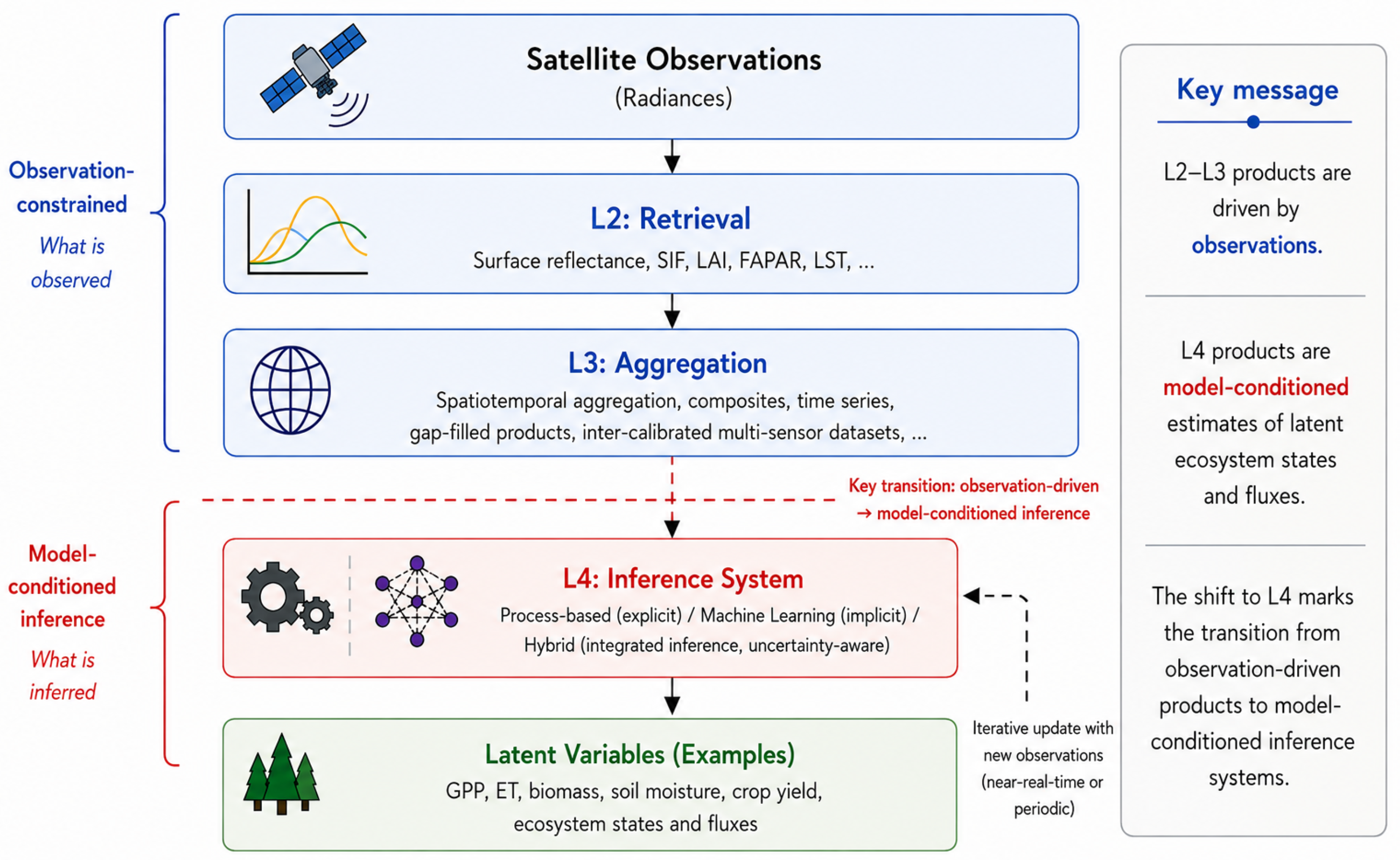
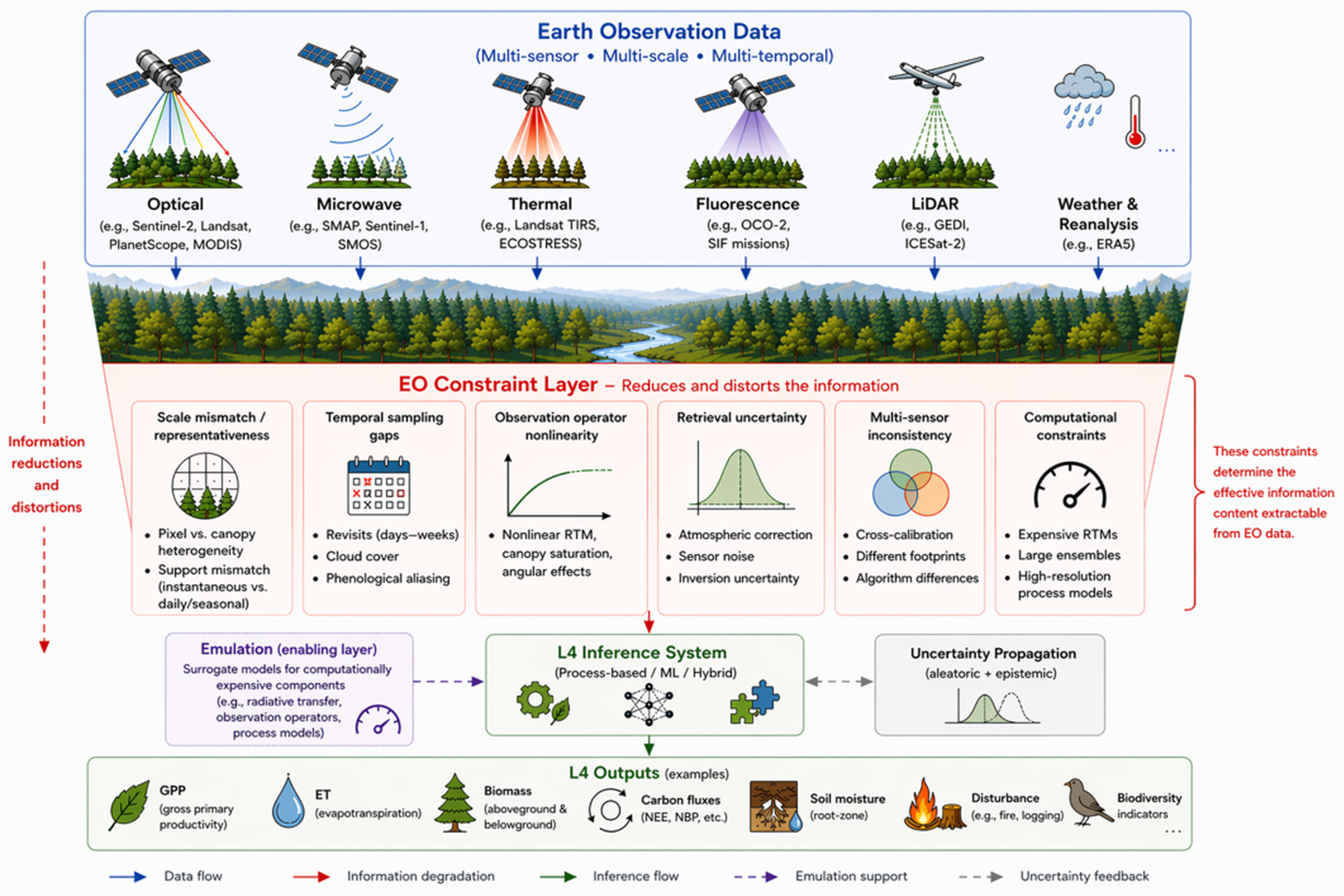
The distinction between L4 and lower-level EO products is not simply one of processing complexity, but of epistemic status. L2 and L3 products remain closely tied to the observational chain: they are derived from measured radiances through atmospheric correction, inversion, compositing, or aggregation, and thus retain a predominantly observation-driven character (see reviews [1,43]). In contrast, L4 products are model-derived variables that require temporal propagation, process representation, or both, and are therefore inherently model-conditioned [15,24]. To clarify this distinction, Figure 1 illustrates the transition from observation-driven EO products (L2–L3) to L4 inference systems, highlighting how latent ecosystem states and fluxes are estimated through integrated observation–retrieval–model inference systems.

More fundamentally, many target variables are only partially observable from EO data. Even when variables such as LAI or SIF provide strong observational constraints [5], or when spectral proxies are used (e.g., [8,44]), key quantities such as fluxes, biomass, or yield must be reconstructed from models linking current observations to past states and system dynamics (e.g., [9,12,13,14]). As a result, L4 products should be interpreted as model-conditioned estimates that depend not only on observations, but also on model structure, parameterization, scale, and uncertainty assumptions (e.g., [15,16,17,24,38]). This dependency arises because EO data provide only indirect and incomplete constraints on the underlying system, requiring models to bridge spatial, temporal, and process-level gaps in the information.

While this inverse-problem formulation is explicit in process-based assimilation frameworks, it also underlies ML and hybrid frameworks in implicit or partially explicit form, where the relationship between EO data and target variables is not prescribed by mechanistic process formulations, but emerges from data-driven inference conditioned by training data, model structure, and prior assumptions. Consequently, agreement with EO inputs alone is not a sufficient indicator of validity. Distinct modelling frameworks may reproduce the same observed variables while diverging substantially in latent states, parameters, or fluxes. Observational consistency is therefore necessary, but not sufficient, for L4 reliability.

Classes of L4 Products and Their Estimation Requirements

L4 products can be broadly categorized into three classes according to the nature of the variables they represent:

• State variables, such as biomass or soil carbon pools, which describe the condition of the ecosystem at a given time.
• Flux variables, such as GPP, ET, or net carbon exchange, which describe rates of exchange between vegetation, soil, and the atmosphere.
• Trajectory variables, such as phenological development or seasonal productivity patterns, which describe temporal evolution.

These categories differ in their dependence on temporal propagation and model structure. State variables can sometimes be approximated from single-date EO observations, but their estimation remains model-dependent, relying on retrieval assumptions, prior information, and scale representations [1,38,45]. Fluxes and trajectories are likewise model-dependent, but depend more strongly on temporal integration and dynamical process representation, as they emerge from time-evolving interactions, interacting controls, and system memory [12,13,14,15]. In practice, this implies that the inference framework is an integral part of the product definition.

Table 2. Representative L4 vegetation products, their classification, main EO and ancillary inputs, common inference strategies, typical challenges, and key references. EO and ancillary inputs include direct measurements (e.g., surface reflectance, LST, microwave signals), retrieved variables (e.g., LAI, FAPAR), derived features (e.g., vegetation indices), and non-EO drivers (e.g., meteorological forcing), reflecting their role across different inference approaches.

L4 Variable	L4 Class	Typical EO and Ancillary Inputs	Inference Strategies	Typical Challenges	Representative References
Gross primary productivity (GPP)	Flux	SIF; FAPAR; LAI; VIs; surface reflectance; meteorology	Light-use efficiency (LUE) models (semi-empirical); LSM/DGVM data assimilation (process-based); ML upscaling (data-driven); hybrid SIF-constrained inference (process–ML)	Uncertainty in absorbed radiation and light-use efficiency; nonlinear SIF–GPP coupling; temporal consistency; scale mismatch; uncertainty propagation across the observation–model chain	Running et al. [8], Jung et al. [12], Nelson et al. [14], Reyes-Muñoz et al. [46]
Evapotranspiration (ET)	Flux	LST; surface reflectance; VIs; LAI/FAPAR; soil moisture; meteorology	Energy-balance models (process-based); LSM data assimilation; ML upscaling/regression (data-driven)	Land–atmosphere coupling; partitioning between soil evaporation and transpiration; heterogeneity; representativeness error; cross-scale consistency	Mu et al. [32], Miralles et al. [33], Jung et al. [47]
Aboveground biomass	State	SAR backscatter; LiDAR-derived canopy height/structure where available; surface reflectance; VIs; land cover	Empirical/allometric scaling models; DGVM simulations (process-based); ML regression (data-driven); multi-sensor data fusion (hybrid)	Signal saturation; structural heterogeneity; limited calibration data; disturbance history; scale transferability	Santoro et al. [34], Saatchi et al. [48], Baccini et al. [49], Tian et al. [50]
Crop yield	State	LAI; VIs; surface reflectance; crop type/area; meteorology	Crop growth model assimilation (process-based); statistical or ML regression (data-driven); hybrid process–ML models	Management effects; cultivar and harvest-index variability; parameter uncertainty; regional transferability; sensitivity to extreme events	Lobell et al. [51], Jeong et al. [52], van Klompenburg et al. [53], Meghraoui et al. [54]
Root-zone soil moisture	State	Microwave soil moisture/brightness temperature; LST; meteorological forcing (including precipitation); vegetation optical depth or land cover	Land surface data assimilation (process-based); hydrological modelling; ML estimation (data-driven)	Depth representativeness; vegetation and roughness effects on microwave observations; observation-operator uncertainty; mismatch between surface and root-zone dynamics	Reichle et al. [16,55,56]
Carbon stocks (soil and vegetation)	State	Biomass maps; SAR/LiDAR structural information; land cover; climate and soil covariates	DGVM simulations (process-based); carbon-cycle modelling; inventory-constrained mapping; ML upscaling (data-driven)	Structural model uncertainty; long-term consistency; sparse reference constraints; disturbance and land-use history; separation of vegetation and soil carbon pools	Sitch et al. [19], Santoro et al. [34], Sitch et al. [57]
Net ecosystem exchange (NEE) and component fluxes (GPP, ecosystem respiration)	Flux	Atmospheric CO2; meteorology; vegetation-state constraints such as LAI/FAPAR for biosphere priors	Atmospheric inversion and carbon-cycle data assimilation (process-based); flux-tower-based ML upscaling (data-driven)	Atmospheric transport uncertainty; attribution ambiguity in partitioning NEE into GPP and respiration; scale mismatch; model dependence of flux separation	Nelson et al. [14], Rayner et al. [58], Byrne et al. [59]
Phenology/productivity trajectories	Trajectory	Time series of VIs; LAI/FAPAR; surface reflectance	Time-series analysis (e.g., TIMESAT); process-based simulations (CGM/LSM); sequence ML models (data-driven)	Temporal gaps; noise; scale-dependent definitions; sensitivity to compositing and smoothing; distinction between greenness and physiological activity	Jönsson and Eklundh [60], Verbesselt et al. 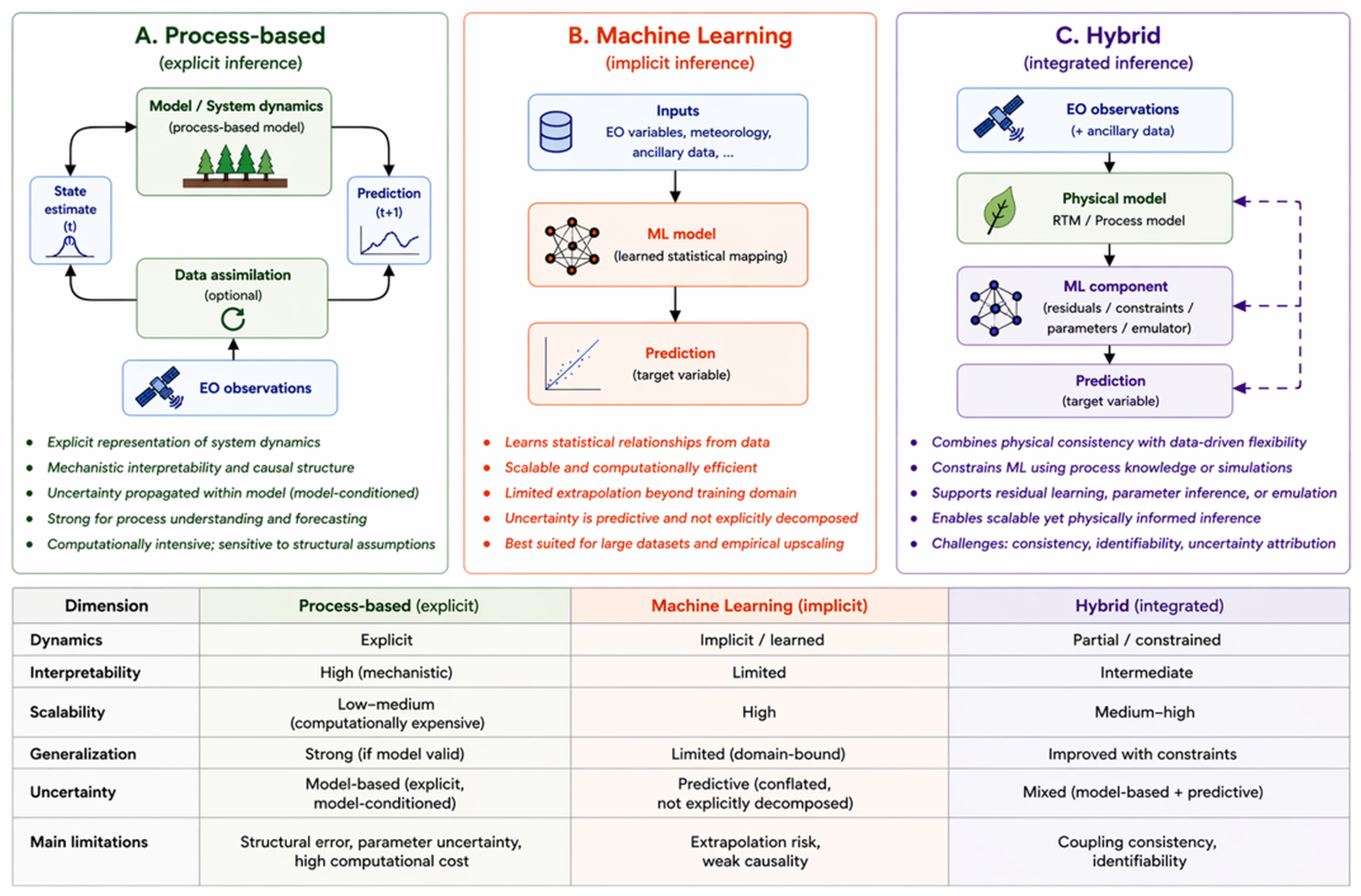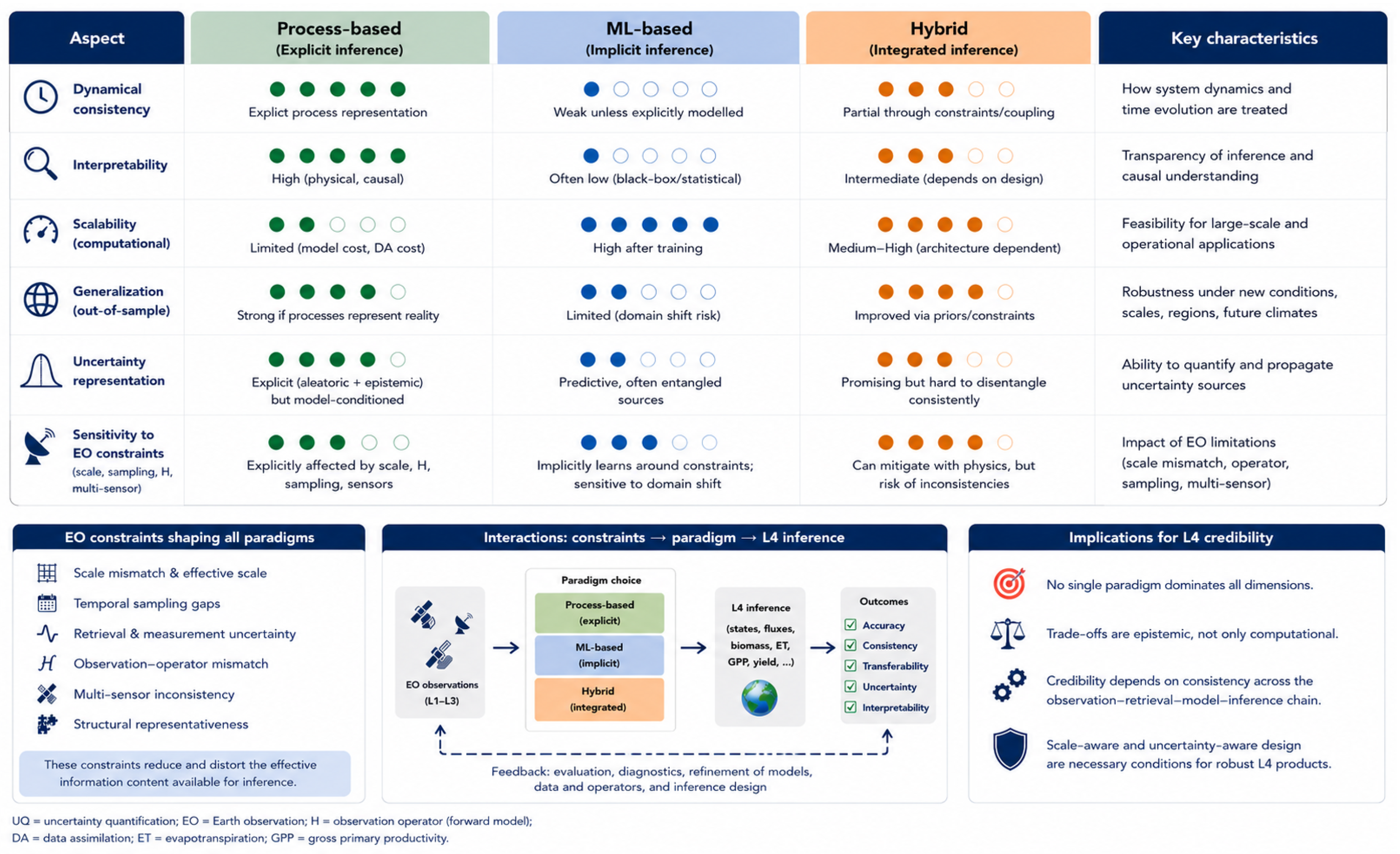[61], Belda et al. [62]

summarizes representative L4 variables, their classification into state, flux, and trajectory types, their main EO inputs, common inference strategies, and typical challenges. The table illustrates that most L4 products are constrained by multiple EO data streams and rely critically on how observational information is linked to model structure through the inference design. Across all classes, L4 products do not constitute a simple extension of retrieval workflows but arise from coupled observation–model inference in which observational information, model dynamics, scale, and uncertainty assumptions jointly determine the estimates. Differences between L4 products therefore reflect variations in modelling assumptions, observation operators, and scale treatment as much as differences in input data. These dependencies reinforce that L4 products are model-conditioned estimates rather than direct observations, and that their reliability is governed by the coherence of the full observation–model–inference chain. Against this background, Figure 2 summarizes the three main approaches for L4 inference—process-based, ML, and hybrid frameworks—and highlights their fundamental differences in dynamics representation, interpretability, scalability, generalization, and uncertainty treatment.

The following sections examine how distinct modelling approaches address this estimation problem and how their assumptions interact with EO-specific constraints, which ultimately define the effective information content available for L4 inference.

3. Process-Based Modelling: Conceptual Foundations and Data Assimilation

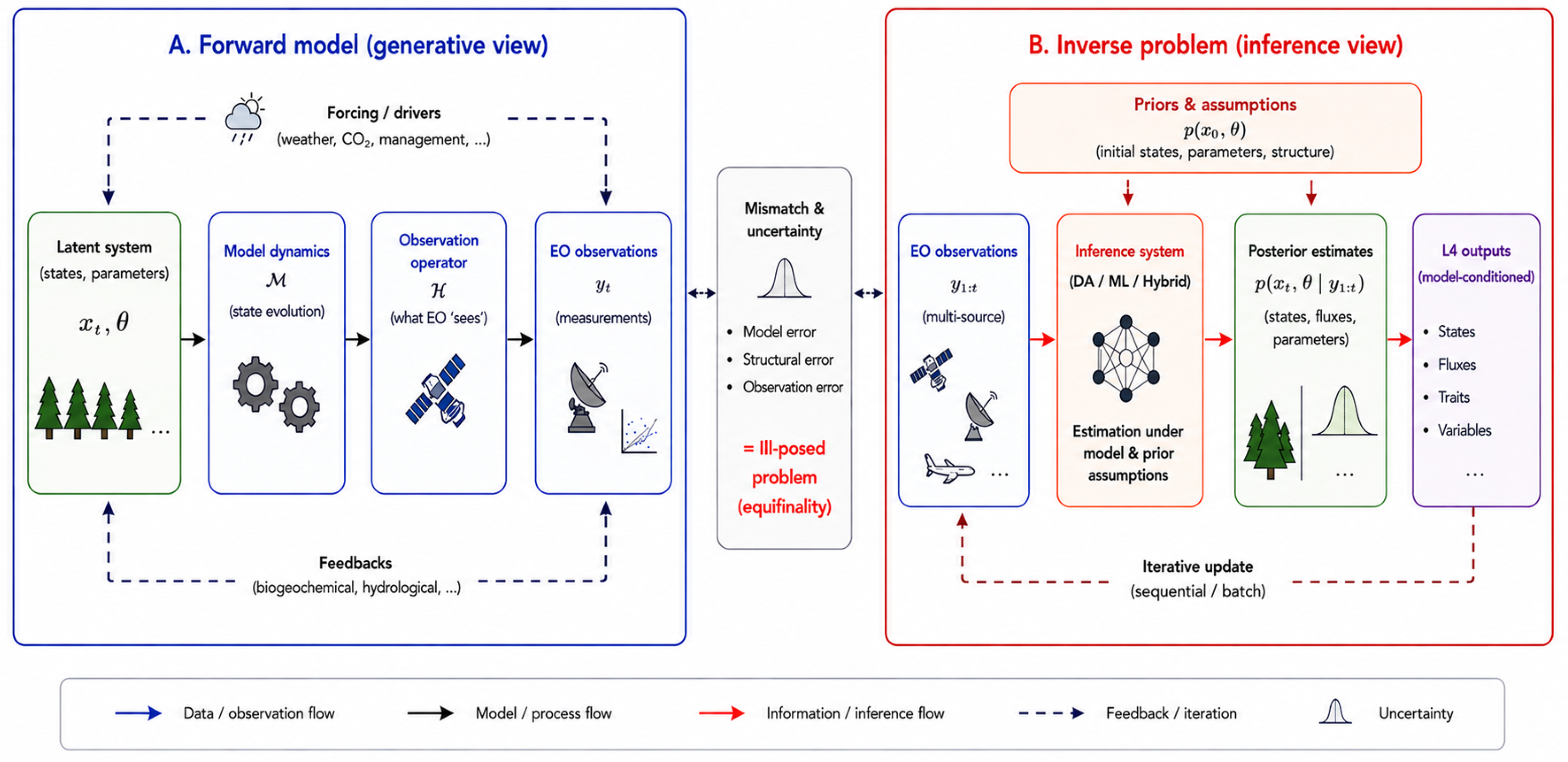
Process-based modelling provides the primary framework for representing ecosystem dynamics in L4 inference, typically through LSMs, CGMs, or DGVMs. Data assimilation offers the most explicit framework for combining EO observations with process-based model dynamics under quantified uncertainty (e.g., [15,16,17,24,63]). In this context, assimilation can be interpreted as Bayesian updating in a state–space system, consistent with Bayesian inverse formulations, in which EO data provide partial and indirect constraints on latent ecosystem states and parameters evolving through time (e.g., [25,64]). To make this formulation explicit, Figure 3 contrasts the forward (generative) and inverse (inference) views of EO-based L4 inference, illustrating how observational constraints are mediated through model dynamics, observation operators, and prior assumptions, and why L4 inference must be interpreted as an ill-posed inverse problem.

The inverse formulation highlights that the information available for L4 inference is fundamentally constrained by the characteristics of EO data and their interaction with model structure. In this sense, the limits of L4 inference arise not from data availability alone, but from the effective information content of EO data, which depends on observation characteristics, scale, and their coupling with the model. These constraints are examined explicitly in Section 6.

Assimilation systems combine three core components: (i) model dynamics driven by external forcing, (ii) observation operators linking model states to EO data, and (iii) analysis updates that integrate prior estimates with observations under explicit uncertainty assumptions. The interaction between these components determines how observational information enters the system and how model structure regularizes the estimation problem (see reviews [28,65]).

In terrestrial EO, data assimilation builds on a long tradition in geophysical sciences, particularly in meteorology and oceanography, where observations are integrated with dynamical models for state estimation and forecasting (e.g., [15,24]). These concepts have been extended to land-surface and biosphere systems, where EO observations—often in the form of L2 products or directly as radiances, such as soil moisture, LST, vegetation traits, and atmospheric CO₂—are assimilated to constrain surface fluxes and ecosystem states (e.g., [16,17,63]). Their implementation in EO-based applications is, however, strongly conditioned by observation uncertainty, measurement–model mismatch, and structural assumptions in the underlying model (e.g., [66]).

Within this broader context, carbon cycle data assimilation systems (CCDAS) represent a prominent class of approaches within the broader family of land–surface data assimilation frameworks [58,67,68,69]. Related developments include implementations within major land surface models such as ORCHIDEE [70], JULES [71], and CLM [72], as well as atmospheric inversion systems that constrain surface fluxes using CO₂ observations [73]. Together, these approaches establish a central perspective adopted throughout this review: L4 products are best understood not as directly retrieved quantities, but as model-conditioned estimates emerging from coupled observation–model inference.

More recent developments extend these concepts toward multi-stream data assimilation frameworks that jointly integrate heterogeneous EO constraints within unified land-surface modelling systems [17,63]. Examples include next-generation coupled vegetation models explicitly designed for multi-stream assimilation, such as the D&B framework, which combines DALEC [74] and BETHY [75] components to jointly assimilate carbon, water, and energy-related observations [21]. Similar developments are emerging in crop growth modelling, where EO-driven data assimilation frameworks integrate vegetation, soil moisture, and meteorological observations to constrain crop states and yield predictions (see reviews [76,77]). In parallel, operational systems such as SMAP L4 demonstrate the integration of microwave soil moisture observations within land surface models to estimate root-zone states and fluxes [16,55]. These developments reflect a transition from single-variable assimilation toward integrated inference architectures that explicitly address cross-variable coupling, observation coupling, and uncertainty propagation.

A defining challenge in terrestrial EO assimilation lies in the indirect and scale-dependent nature of the observations. EO measurements typically reflect radiative processes rather than the target ecosystem states or fluxes, and their information content is strongly modulated by viewing geometry, atmospheric effects, and sub-pixel heterogeneity. As a result, the relationship between observations and model variables is highly nonlinear, scale-dependent, and often weakly constrained. This requires the explicit representation of observation physics through observation operators, such as radiative transfer and energy balance models, and careful treatment of scale mismatches between observations and model states. Consequently, the resulting estimation problem is therefore intrinsically ill-posed, with multiple plausible solutions consistent with the available observations (e.g., [38,64,78,79,80,81]).

This structure can be formalized by distinguishing two key components of the inference problem. The observation operator $\mathcal{H}$ links EO data to model variables, while the model operator $\mathcal{M}$ defines the underlying system dynamics that constrain the estimation. In this framework, $\mathcal{H}$ governs how observational information enters the system, whereas $\mathcal{M}$ determines how this information is propagated and regularized through dynamical and structural assumptions. In terrestrial applications, $\mathcal{M}$ is typically implemented through process-based models that encode prior knowledge of ecosystem functioning and temporal evolution. While these models provide essential constraints, they also introduce structural assumptions that strongly condition posterior estimates.

These considerations highlight the central role of process-based models in defining the dynamical structure of L4 inference.

Table 3. Representative process-based models used in EO-based L4 inference, including their main characteristics, roles in inference, and typical EO constraints assimilated through observation operators.

Model Class	Examples	Key Characteristics	Typical EO Constraints (via Observation Operators)	Representative References
Land surface/terrestrial biosphere models	CLM, JULES, ORCHIDEE, BESS	Simulate coupled carbon, water, and energy fluxes driven by meteorological forcing; represent land–atmosphere interactions; provide dynamic state propagation for L4 inference	LAI, FAPAR, soil moisture, LST	Krinner et al. [70], Clark et al. [71], Lawrence et al. [72], Li et al. [82]
Dynamic global vegetation models (DGVMs)	LPJ, LPJ-GUESS	Represent vegetation dynamics, biogeography, and long-term carbon cycling using plant functional types, disturbance, and succession processes	FAPAR, biomass proxies, atmospheric CO2	Sitch et al. [19], Smith et al. [83], Sitch et al. [84]
Carbon cycle data assimilation systems (CCDAS)	BETHY, CCDAS frameworks	Variational or Bayesian assimilation of EO and atmospheric observations into carbon cycle models; joint state–parameter estimation with explicit uncertainty propagation	FAPAR, atmospheric CO2, SIF	Rayner et al. [58], Kaminski et al. [68], Scholze et al. [69]
Crop growth models	DSSAT, APSIM, WOFOST, AquaCrop	Simulate crop phenology, growth, and yield based on physiological processes, environmental forcing, and management practices; often coupled with assimilation or calibration	LAI, VIs, SIF, soil moisture	Jones et al. [85], Keating et al. [86], van Diepen et al. [87], Steduto et al. [88], de Wit et al. [89]
Hydrological models	VIC, PCR-GLOBWB	Simulate terrestrial water balance, runoff generation, and soil moisture dynamics; support L4 inference of water-related states and fluxes	Soil moisture, ET, precipitation proxies	Liang et al. [90], Van Beek et al. [91], Bierkens [92]
Surface energy balance models	SEBAL, TSEB	Estimate surface energy fluxes using radiative and thermal constraints; typically applied diagnostically or as components in ET inference frameworks	LST, reflectance	Bastiaanssen et al. [93], Norman et al. [94]
Canopy RTM–process models	SCOPE; DART; LESS	Couple radiative transfer, photosynthesis, and energy balance (SCOPE), or explicitly represent 3D canopy structure and radiative processes (DART, LESS), providing physically consistent links between optical/thermal signals and vegetation functioning; used as observation operators or to generate synthetic training data	SIF, reflectance, thermal signals	van der Tol et al. [79], Yang et al. [80], Gastellu-Etchegorry et al. [95], Qi et al. [96]

summarizes representative model classes commonly used in EO-based L4 estimation, illustrating how distinct modelling frameworks encode system dynamics and interact with EO-derived constraints through observation operators, ranging from land-surface and vegetation models to crop, hydrological, and canopy RTM–process models [19].

3.1. State–Space Formulation and the Role of Observation Operators

Assimilation problems are commonly expressed as:

$${\mathbf{x}}_t=\mathcal{M}({\mathbf{x}}_{t-1},{\mathbf{u}}_t,\mathit{\theta })+{\eta }_t,$$

(1)

$${\mathbf{y}}_t=\mathcal{H}({\mathbf{x}}_t,\mathit{\theta })+{ϵ}_t,$$

(2)

where ${\mathbf{x}}_t$ is the system state, $\mathcal{M}$ is the model operator, ${\mathbf{u}}_t$ denotes external forcing, $\mathit{\theta }$ represents parameters, and $\mathcal{H}$ is the observation operator that maps latent states to EO-observable quantities. In EO-based applications, the observation operator $\mathcal{H}$ is a central source of complexity and uncertainty because satellite sensors do not observe state variables directly, but radiometric or thermal signals emerging from the interaction of canopy structure, soil background, atmospheric effects, viewing geometry, and radiative transfer processes (e.g., [1,64,78,79]). As a result, $\mathcal{H}$ is nonlinear, partially non-invertible, and strongly scale-dependent, linking EO data to model variables only indirectly.

This has direct implications for L4 inference. Observational constraints derived from variables such as LAI, FAPAR, SIF, LST, or soil moisture are inherently incomplete and provide only partial and indirect information on the target variables. Consequently, L4 inference constitutes an ill-posed inverse problem, in which the available EO data are insufficient to uniquely and robustly constrain the underlying states and fluxes. As a result, identifiability is limited, and equifinality arises, whereby multiple combinations of states, parameters, and model structures can reproduce the same observations, preventing a unique and physically consistent solution [21,64,68]. Posterior estimates therefore remain strongly conditioned by modelling assumptions.

The interaction between $\mathcal{H}$ and $\mathcal{M}$ therefore defines the effective information transfer from EO data to latent system states. While $\mathcal{H}$ determines how observational information enters the system, $\mathcal{M}$ constrains its propagation through dynamical and structural assumptions. From an L4 perspective, assimilation does not resolve the ill-posed nature of the inverse problem, but redistributes it across observation operators, model structure, and prior assumptions, making compatibility between these components a primary determinant of product reliability, rather than eliminating ambiguity in the inference itself.

3.2. Uncertainty Sources and Methodological Implications

Uncertainty plays a central role in L4 inference, reflecting the ill-posed nature of the estimation problem and the limited and indirect constraints provided by EO data. In EO-based L4 systems, uncertainty arises from multiple sources, including measurement noise, atmospheric correction, retrieval errors, forcing uncertainty, parameter uncertainty, representativeness effects, and structural model error (e.g., [17,63,97]). These sources can be broadly grouped into two categories: (i) aleatoric uncertainty, associated with irreducible uncertainty in observations and forcing data, and (ii) epistemic uncertainty, arising from incomplete knowledge of model structure, parameterization, and retrieval models. Representativeness effects caused by mismatches between the scale and definition of observations and model states modify both uncertainty components and become increasingly important towards L3 and L4 inference (e.g., [97,98]).

In terrestrial EO applications, uncertainty associated with model structure and representativeness often exceeds that arising from measurement noise. Sub-pixel heterogeneity, inconsistencies between observation and model resolution, and simplifications in observation operators introduce systematic discrepancies that cannot be resolved by increasing sensor precision alone. Consequently, uncertainty in L4 estimates is primarily conditioned by model assumptions and observation–model compatibility rather than by instrument noise (e.g., [15,97]). The dominance of model-related epistemic uncertainty, together with representativeness uncertainty, has direct implications for the formulation of data assimilation systems. Assimilation algorithms differ not only in their computational properties, but also in how uncertainty is represented and updated within the inference process. Variational approaches (e.g., 3D-Var, 4D-Var) rely on prescribed error covariance structures and often assume Gaussian error statistics, placing strong emphasis on prior specification and internally consistent model dynamics (e.g., [24,28]). Ensemble-based methods (e.g., Ensemble Kalman Filter (EnKF), particle filters) estimate uncertainty from the evolving ensemble and can better accommodate nonlinear and non-Gaussian behaviour, at the cost of sampling limitations and increased computational demand (e.g., [24,99]).

A range of assimilation algorithms has been developed within EO-based L4 inference frameworks (

Table 4. Representative data assimilation methods used in EO-based L4 inference, highlighting their formulation, strengths, limitations, and their role in representing and updating uncertainty within EO-constrained inference.

Method	Key Characteristics	Main Strengths	Main Limitations	Key References
3D-Var	Variational assimilation at a single time step; minimizes a cost function combining observations and prior state using prescribed (static) error covariances; limited representation of temporal evolution	Efficient; robust; relatively simple implementation	Static covariances limit representation of flow-dependent and scale-dependent errors; no explicit temporal propagation of information	Reichle [15], Lorenc [100]
4D-Var	Variational assimilation over a time window; optimizes the initial state such that the model trajectory fits observations using model dynamics and observation operators; requires adjoint model for gradient computation	Dynamical consistency; efficient use of temporal information; physically constrained trajectories	High computational cost; requires adjoint model; sensitivity to model structural and observation-operator errors	Evensen [24], Lewis et al. [64]
EnKF	Sequential ensemble-based filtering; propagates an ensemble of model states forward in time and updates using observations; error covariances estimated from the ensemble (flow-dependent)	Scalable; naturally uncertainty-aware; no adjoint required; suitable for nonlinear and high-dimensional systems	Sampling error due to limited ensemble size; requires localization and inflation; challenges with strongly nonlinear observation operators	Reichle [15], Evensen [101]
Particle filter	Fully nonlinear Bayesian filtering; represents posterior distribution with weighted particles; no Gaussian assumptions; suitable for strongly nonlinear and non-Gaussian systems	Flexible posterior representation; theoretically exact Bayesian inference	Computationally prohibitive in high-dimensional systems; weight degeneracy; limited scalability for EO applications	van Leeuwen [102]
Hybrid EnKF–Var	Combines ensemble-derived flow-dependent covariances with static variational covariances; integrates ensemble information within variational frameworks	Improved covariance representation; balances robustness of variational methods with adaptability of ensembles	Complex implementation; tuning of hybrid weights; increased computational demand; potential inconsistencies between components	Hamill and Snyder [103], Wang et al. [104]
Ensemble smoother	Ensemble-based assimilation over temporal windows; updates states and/or parameters using observations across multiple time steps (smoothing rather than filtering)	Efficient parameter estimation; reduced computational cost compared to full 4D-Var; suitable for offline or retrospective analysis	Limited real-time applicability; assumes temporal consistency over the window; may smooth out rapid dynamics and extremes	Evensen [24], Emerick and Reynolds [105]

). These methods differ primarily in how they represent and update uncertainty within the inference process. For L4 inference, however, the choice of algorithm is secondary to the compatibility between model dynamics, observation operators, and uncertainty representation. From a methodological perspective, uncertainty is therefore not an auxiliary output of L4 inference, but a defining element of the estimation framework itself. Its representation governs how observational information is weighted against model dynamics and prior assumptions, and thus directly conditions the resulting state and flux estimates. This view is consistent with classical inverse theory, in which state and parameter estimation are formulated as Bayesian inference problems under prior and observational constraints [25].

4. Machine Learning Approaches

ML frameworks provide an alternative pathway to L4 inference, in which latent ecosystem variables are inferred from data through statistical relationships between EO data, ancillary predictors, and target variables. Unlike process-based assimilation, these approaches do not explicitly represent system dynamics or state–space evolution, but instead learn such relationships directly from data (e.g., [12,13,14,106,107,108]). As a result, L4 inference shifts from physically constrained state estimation toward training-domain-dependent prediction, in which system dynamics are not explicitly represented but only indirectly reflected through correlations present in the training data [109].

Building on this perspective, L4 products represent the outcome of implicit inference systems, in which information from EO observations, meteorological forcing, and reference datasets (e.g., eddy covariance measurements) is integrated through training (e.g., [13,14,35,108]). The resulting models encode statistical relationships that approximate the observation–process–response chain, but without explicitly representing the underlying mechanisms or enforcing dynamical consistency (e.g., [31,106]). Prominent examples include global upscaling frameworks such as FLUXCOM, UFLUX as well as EO-based models for crop yield, ET, and soil moisture, which demonstrate the capability of ML methods to capture large-scale ecosystem variability from EO and climate predictors (e.g., [12,14,110]).

A central difference from process-based approaches is that ML-based products are governed primarily by the joint distribution represented in the training data rather than on explicit process knowledge. This enables high predictive flexibility, but also makes the resulting inference strongly dependent on data coverage, sampling design, and the stability of learned relationships under changing conditions. Table 5 summarizes representative ML methods used for EO-based L4 estimation, together with their typical applications, strengths, and limitations.

4.1. Strengths: Flexibility, Nonlinear Representation, and Scalability

A major strength of ML lies in its ability to represent complex nonlinear relationships among heterogeneous predictors without requiring explicit process formulations (see reviews [1,26]). In the L4 context, this enables the integration of EO variables, meteorological forcing, soil properties, and land-cover information within data-driven estimation frameworks [13,14]. Such approaches have demonstrated strong predictive performance across large spatial domains in applications including global flux estimation, crop yield prediction, and hydrological variable mapping (e.g., [9,12,111]), with recent developments further extending these capabilities toward more consistent and scalable inference systems (e.g., [14,108,110]). Once trained, ML models provide fast prediction, making them particularly well suited for large-scale and cloud-based EO processing pipelines. This computational efficiency supports operational production of L4 products at global scale, often with high temporal frequency.

Probabilistic ML methods can also provide predictive uncertainty estimates. ML methods such as Gaussian process regression (GPR), ensemble learning, and Bayesian neural networks offer quantification of predictive spread, which is valuable for large-scale mapping (e.g., [108,112,113]). Such uncertainty estimates primarily characterize epistemic uncertainty associated with the statistical model and training data, rather than explicitly representing uncertainty arising from ecosystem processes or process–model dynamics. Such methods are increasingly used to provide uncertainty-aware L4 products, although this uncertainty typically reflects predictive variability rather than a physically interpretable decomposition of uncertainty sources (e.g., [97,112]).

Table 5. Representative ML methods for EO-based L4 inference, focusing on latent ecosystem variables (e.g., fluxes, biomass, yield), their strengths, and limitations under EO constraints.

Method	Typical L4 Applications	Strengths	Limitations	Representative References
Ensemble-based methods (e.g., Random Forest, Gradient Boosting, model stacking)	GPP, ET, energy fluxes (e.g., FLUXCOM and RF-based upscaling)	Robust; captures nonlinear relationships; scalable to large EO datasets; handles heterogeneous predictors; improved predictive performance through aggregation of multiple models or learners	Limited extrapolation beyond training domain; weak physical interpretability; predictive uncertainty is generally not attributable to distinct physical uncertainty sources	Jung et al. [12], Tramontana et al. [13], Nelson et al. [14], Zeng et al. [114]
Gaussian Process Regression (GPR; kernel-based probabilistic methods)	GPP, carbon fluxes, SIF-based productivity	Probabilistic predictions; explicit uncertainty quantification; effective with limited training data	Computational scaling with dataset size; dependence on training domain; kernel design sensitivity	Reyes-Muñoz et al. [46,108], De Clerck et al. [115]
Artificial Neural Networks (ANN; shallow feedforward networks)	Crop yield, biomass, GPP	Flexible nonlinear function approximation; computationally efficient; widely used in early EO-based upscaling and yield modelling	Limited interpretability; risk of overfitting; uncertainty not inherently represented; limited extrapolation under domain shift	Beer et al. [9], van Klompenburg et al. [53], Kaul et al. [116], Jung et al. [117]
Deep Learning (CNN, RNN, Transformers, foundation models)	Global fluxes (GPP, ET), crop yield, and spatiotemporal ecosystem dynamics	Captures spatial and temporal dependencies; high predictive performance; suitable for large EO data streams and data cubes	Data-intensive; limited extrapolation under domain shift; opaque uncertainty representation	Reichstein et al. [29], Rolnick et al. [107], Jabed and Murad [111], Muruganantham et al. [118]

Table 5. Representative ML methods for EO-based L4 inference, focusing on latent ecosystem variables (e.g., fluxes, biomass, yield), their strengths, and limitations under EO constraints.

Method	Typical L4 Applications	Strengths	Limitations	Representative References
Ensemble-based methods (e.g., Random Forest, Gradient Boosting, model stacking)	GPP, ET, energy fluxes (e.g., FLUXCOM and RF-based upscaling)	Robust; captures nonlinear relationships; scalable to large EO datasets; handles heterogeneous predictors; improved predictive performance through aggregation of multiple models or learners	Limited extrapolation beyond training domain; weak physical interpretability; predictive uncertainty is generally not attributable to distinct physical uncertainty sources	Jung et al. [12], Tramontana et al. [13], Nelson et al. [14], Zeng et al. [114]
Gaussian Process Regression (GPR; kernel-based probabilistic methods)	GPP, carbon fluxes, SIF-based productivity	Probabilistic predictions; explicit uncertainty quantification; effective with limited training data	Computational scaling with dataset size; dependence on training domain; kernel design sensitivity	Reyes-Muñoz et al. [46,108], De Clerck et al. [115]
Artificial Neural Networks (ANN; shallow feedforward networks)	Crop yield, biomass, GPP	Flexible nonlinear function approximation; computationally efficient; widely used in early EO-based upscaling and yield modelling	Limited interpretability; risk of overfitting; uncertainty not inherently represented; limited extrapolation under domain shift	Beer et al. [9], van Klompenburg et al. [53], Kaul et al. [116], Jung et al. [117]
Deep Learning (CNN, RNN, Transformers, foundation models)	Global fluxes (GPP, ET), crop yield, and spatiotemporal ecosystem dynamics	Captures spatial and temporal dependencies; high predictive performance; suitable for large EO data streams and data cubes	Data-intensive; limited extrapolation under domain shift; opaque uncertainty representation	Reichstein et al. [29], Rolnick et al. [107], Jabed and Murad [111], Muruganantham et al. [118]

The comparison in Table 5 shows that ML-based L4 inference is primarily applied to fluxes and integrative ecosystem variables such as GPP, ET, biomass, and crop yield. Across methods, a key strength is the ability to learn nonlinear relationships from heterogeneous EO and ancillary data, enabling accurate mapping across large spatial domains. A principal limitation is the dependence on training data representativeness, which constrains extrapolation under changing environmental conditions. Moreover, probabilistic ML methods can quantify epistemic uncertainty associated with the learned model, although this uncertainty is generally not attributable to specific physical sources such as process, parameter, or observation uncertainty.

4.2. Limitations: Domain Dependence, Weak Physical Consistency, and Ambiguous Uncertainty

The limitations of ML-based L4 inference arise directly from its data-driven nature. ML models learn statistical relationships rather than transferable process representations, and therefore provide no guarantee of physical consistency or causal validity outside the training domain (e.g., [12,13,29,30,31,107]). In EO-based flux estimation, these learned relationships approximate observation–response behaviour without explicitly representing underlying ecosystem processes [13,14]. Their validity is consequently constrained by the representativeness of the training data, including the coverage of environmental conditions and observation space [12,14]. Extrapolation to unseen conditions (e.g., climate extremes or land-cover change) can therefore lead to unreliable predictions, reflecting sensitivity to domain shift in data-driven L4 systems [14].

Second, ML methods generally lack explicit representation of system dynamics. While temporal models can capture sequential dependencies, they generally do not enforce conservation laws, process-level coupling, or coherence between instantaneous predictions and evolving system states. This means that predictions may be locally accurate while remaining inconsistent across time or related variables [30,31].

Third, ML-derived predictive uncertainty is often difficult to interpret in physical terms. These estimates typically conflate epistemic (model) and aleatoric (data) components without clear separation. In EO applications, predictive uncertainty is therefore often dominated by epistemic contributions associated with model structure, training-data limitations, and domain shift, particularly outside the training domain (see review [97]). Consequently, predictive uncertainty primarily reflects the learned statistical model and its training domain, limiting its direct physical interpretation and comparability with the structured uncertainty propagation provided by assimilation frameworks.

Finally, ML methods inherit scale and representativeness issues from both EO inputs and training datasets. Sampling biases (e.g., flux tower distribution), aggregation effects, and cross-sensor inconsistencies can propagate directly into learned relationships [12,38], with limited mechanisms for diagnosis or correction once embedded. In contrast to process-based approaches, ML methods trade mechanistic consistency for flexibility and scalability. They are particularly effective for large-scale mapping under relatively stable conditions, but are generally less suited for causal interpretation, scenario analysis, and uncertainty-aware dynamical prediction. These limitations motivate the development of hybrid frameworks that combine data-driven flexibility with physically based constraints.

5. Hybrid Process–ML Frameworks

Hybrid modelling approaches aim to reconcile the complementary strengths and limitations of process-based and ML methods to L4 inference [30,31]. In EO-based L4 inference, hybridization is not merely a methodological extension, but a response to an inherent tension: process-based models provide mechanistic consistency and explicit system dynamics, but are often computationally demanding and structurally restrictive, whereas ML methods offer flexibility and scalability, but typically lack physical constraints, causal interpretability, and robust extrapolation capacity.

Hybrid frameworks address this tension by combining learned components with physically informed representations at different stages of the modelling chain (see reviews [1,26,27,31]). This shifts the emphasis from selecting a single paradigm to designing coherent interactions among process knowledge, EO data, and statistical learning. The central challenge is therefore not hybridization itself, but preserving compatibility among learned components, process representations, observation operators, and uncertainty assumptions.

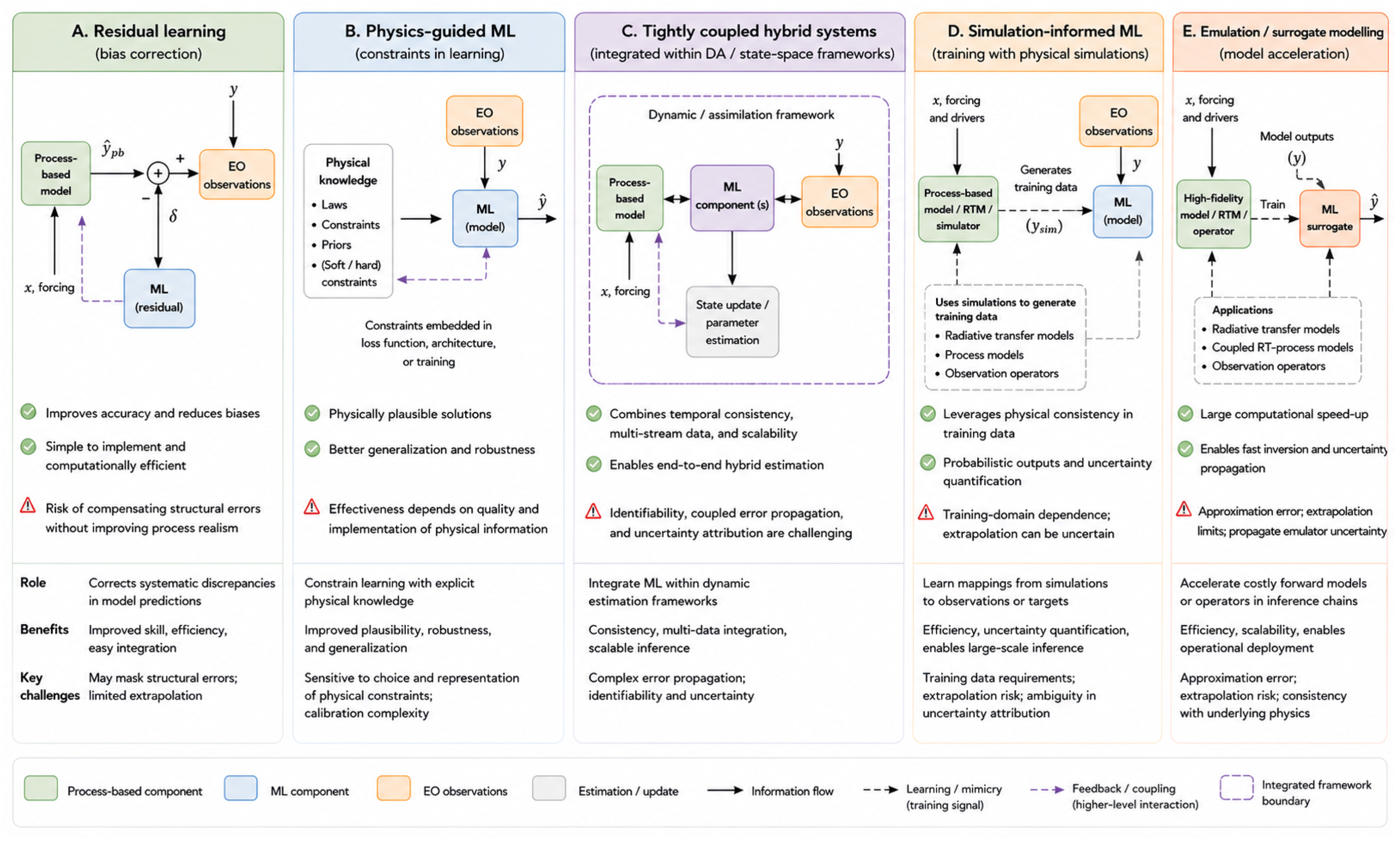
Hybridization can occur at multiple levels of the modelling chain, depending on how physical knowledge and statistical learning are integrated within the inference process. Figure 4 summarizes five representative classes of hybridization in L4 inference, illustrating how these components interact across the modelling workflow. The placement of the ML component is critical, because it determines whether the hybrid system acts primarily as a bias-correction layer, a learning system constrained by physical knowledge, a simulation-informed statistical model, or an integrated estimation framework. Hybridization can also act as a means of accelerating inference, when ML components replace expensive forward models or observation operators. Hybrid approaches therefore form a spectrum of design choices rather than a single modelling framework.

Following the conceptual classification illustrated in Figure 4, hybrid frameworks can be systematically distinguished by where the learned component enters the inference chain and how physical knowledge is incorporated. Residual-learning strategies operate at the output level, correcting systematic discrepancies in process-based predictions (e.g., [39]). Physics-guided approaches impose constraints directly on the learning system, for example through loss functions or architectural design. Simulation-informed strategies instead embed physical knowledge implicitly through training data generated by process-based or radiative transfer models (RTMs). More tightly coupled hybrid systems integrate learned components within dynamic or assimilation frameworks, enabling joint state–parameter inference under multi-stream observational constraints. Finally, emulation or surrogate approaches approximate computationally expensive forward models or observation operators, enabling efficient simulation and inversion within inference workflows. While primarily introduced to improve computational efficiency, emulation can also influence uncertainty propagation and the practical feasibility of large-scale or iterative inference systems (see further Section 8).

These classes differ primarily in where physical knowledge enters the inference chain—within the model formulation, training data, post-processing stage, state-space dynamics, or the computational representation of forward operators—and how it constrains learning and inference. This leads to distinct trade-offs between flexibility and physical consistency. Approaches operating at the output level (e.g., residual learning) may improve predictive performance but risk masking structural model deficiencies through statistical compensation. In contrast, physics-guided and tightly coupled systems seek to enforce alignment within the inference process itself, but introduce additional challenges related to identifiability, coupled error propagation, and the attribution of uncertainty across interacting components.

Recent developments in vegetation EO illustrate the potential of simulation-informed Hybrid frameworks, particularly within the class of simulation-informed ML approaches. For example, hybrid GPR frameworks trained on physically consistent simulations have been used to infer vegetation productivity variables from synergistic combinations of SIF, structural EO variables, and meteorological drivers [46,115]. Such approaches exploit training data derived from coupled radiative transfer and photosynthesis models such as SCOPE [79,80], thereby embedding biophysical consistency within probabilistic statistical estimation. In these frameworks, the physical model is not evaluated during inference, but instead defines the training domain of the statistical model. As a result, physical consistency is incorporated implicitly through the structure of the training data rather than enforced explicitly during prediction.

Despite their potential, hybrid frameworks do not automatically resolve the limitations of either mechanistic or data-driven modelling. They often inherit scale mismatch, representativeness limitations, and structural assumptions from both components. Synthetic training data may fail to span real observational variability, and learned corrections may compensate for process-model deficiencies without resolving them (e.g., [35,38]). Uncertainty may become more difficult to interpret once multiple coupled components interact [97]. Hybridization therefore redistributes, rather than eliminates, uncertainty and identifiability challenges across the modelling chain. In particular, it does not resolve the fundamental identifiability problem of L4 inference, but shifts it across learned and mechanistic components, where ambiguities may become more difficult to diagnose.

Table 6. Representative categories of hybrid modelling for EO-based L4 inference, highlighting how data-driven and process-based components are combined within the inference chain.

Category	Description	Typical EO Applications	Main Challenges	Representative References
Physics-guided ML	Physical constraints are explicitly embedded within the learning process (e.g., loss functions or architectures), enforcing consistency during training and/or inference	Constrained flux estimation; SIF–GPP inference; phenology and productivity modelling	Constraint design; trade-off between flexibility and realism; calibration complexity; sensitivity to constraint formulation	Karpatne et al. [30], Willard et al. [31]
Simulation-informed ML	Statistical models trained on synthetic data generated by physically based models (e.g., RTMs or process models), where physical consistency is implicitly encoded through the training distribution rather than enforced during inference	GPR-based GPP retrieval; uncertainty-aware EO upscaling; SIF–structure–climate inference	Training-domain dependence; limited extrapolation; ambiguity in uncertainty attribution; sensitivity to prior assumptions	Reyes-Muñoz et al. [46], De Clerck et al. [115], Verrelst et al. [119]
Residual learning	ML corrects systematic discrepancies between process-based model outputs and observations as a post-processing or bias-correction layer	Bias correction of GPP/ET; downscaling; post-processing of model-based products	Overfitting; limited transferability; risk of non-physical compensation; lack of interpretability	Willard et al. [31], Zhu et al. [39]
Tightly coupled hybrid systems	Data-driven components embedded within dynamic or assimilation frameworks, enabling joint state–parameter inference under physical constraints	Hybrid state–space models; joint state–parameter estimation; forecasting; multi-stream EO integration	Identifiability; coupled error propagation; computational complexity; consistency across model components	Kumar et al. [17], Li et al. [63]
Emulation/surrogate modelling	ML approximates computationally expensive forward models or observation operators, enabling efficient simulation and inversion within inference workflows	RTM emulation; fast inversion; scalable forward modelling; uncertainty propagation	Approximation error; extrapolation limits; consistency with underlying physics; propagation of emulator uncertainty	Verrelst et al. [119], Rivera et al. [120], Vicent et al. [121]

summarizes representative categories of hybrid modelling for L4 inference and highlights their distinct trade-offs in physical consistency, scalability, interpretability, and uncertainty representation. From this perspective, process-based, ML, and hybrid frameworks are best viewed not as isolated alternatives, but as complementary positions along a continuum between physically constrained and data-driven inference.

From an L4 perspective, the promise of hybrid frameworks lies in their ability to combine physical consistency, observational linkage, and computational scalability within a single modelling architecture. However, this promise depends on the coherence of the hybrid design. Inconsistencies between learned and mechanistic components can lead to error compensation rather than genuine improvement, while poorly aligned scales, priors, or training domains can introduce hidden biases. Rather than eliminating the challenges of L4 inference, hybrid systems redistribute them across interacting model components, where inconsistencies may become more difficult to identify and interpret. Their reliability therefore depends on whether physical constraints, statistical learning, EO observation characteristics, and uncertainty representation are integrated consistently and transparently across the modelling chain. These challenges become particularly pronounced under EO-specific conditions such as scale mismatch, nonlinear observation operators, and limited temporal sampling, which are examined in detail in Section 6.

6. EO Constraints on L4 Inference

EO data provide essential constraints for L4 inference, but also impose fundamental limitations arising from scale, observation physics, and uncertainty. These limitations do not merely affect inference; they define the effective information content of EO data and thus the fundamental limits of what can be inferred. This perspective is consistent with findings from global flux estimation frameworks, where discrepancies across products often reflect differences in modelling assumptions and inference design rather than EO inputs alone [14,19,35]. Importantly, these constraints act across the full EO processing chain—from observation and retrieval (L2), through aggregation and compositing (L3), to model-based inference (L4). Limitations introduced at earlier stages cannot be corrected downstream, but instead shape the entire inference process. To synthesize these effects, Figure 5 conceptualizes how information is progressively transformed from observation (L1–L3) to model-conditioned L4 inference, operationalizing the concept of effective information content introduced earlier.

A fundamental challenge across the L2–L4 processing chain is scale mismatch. Satellite observations integrate signals over heterogeneous areas, while models operate at their own spatial resolution and internal representation. Because radiative transfer and vegetation processes are nonlinear, retrieval and aggregation are not commutative (e.g., [38,81,122]). Consequently, variables retrieved at a given resolution do not necessarily correspond to the aggregated behaviour of the system at finer scales, leading to representativeness errors that propagate through both assimilation and ML-based estimation (e.g., [12,38,81,122,123]). More generally, EO data constrain the system at an effective scale, defined as the scale at which the EO measurement becomes informative about the target variable, emerging from the interaction between sensor characteristics, canopy structure, and nonlinear radiative transfer processes [38]. This effective scale may differ substantially from the nominal pixel resolution and from the support of model variables, leading to inconsistencies across observation, retrieval, and estimation levels that cannot be corrected through post-processing alone. As a result, L4 inference is directly affected, as scale mismatch introduces representativeness errors, limits identifiability, and propagates structural uncertainty into inferred states and fluxes. This limitation is explicitly represented in process-based and many hybrid frameworks through the observation operator $\mathcal{H}$, whereas ML methods typically absorb it implicitly into learned statistical relationships.

Temporal sampling introduces additional constraints. EO data are discrete, irregular, and often affected by cloud contamination, whereas vegetation processes evolve continuously. Estimation systems must therefore rely on model dynamics or learned temporal relationships to bridge these gaps, which can introduce aliasing, temporal smoothing, or delayed responses, particularly for rapidly varying processes such as stress dynamics or phenological transitions (e.g., [60,61,124]). These effects can be partially mitigated in assimilation-based approaches through dynamical propagation, but tend to affect ML frameworks more strongly because of their dependence on temporally representative training data.

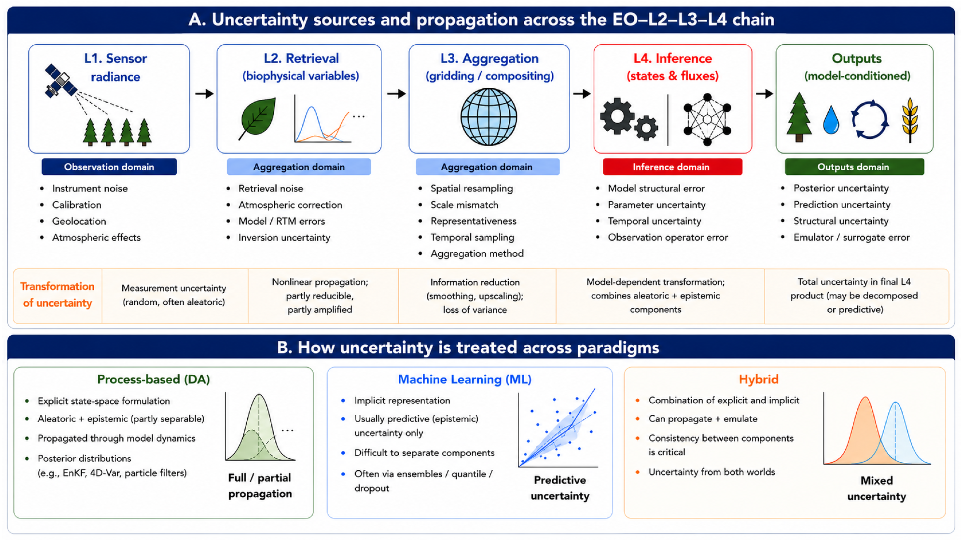
Across the EO processing chain, uncertainty determines how information is transformed and constrained. Building on the uncertainty sources and methodological considerations outlined in Section 3.2, its role is considered across the observation–retrieval–model–inference chain. Rather than acting as an additive error term, uncertainty is continuously reshaped as EO data are retrieved, aggregated, and integrated within model-based inference frameworks. These transformations are generally nonlinear and state-dependent. Both aleatoric and epistemic uncertainty evolve along this chain, although through different mechanisms. Aleatoric uncertainty associated with observations and measurements is propagated and transformed through retrieval, aggregation, and representativeness effects, whereas epistemic uncertainty reflects imperfect model structure, parameterization, and retrieval assumptions, and may either decrease as observations constrain the inference or increase when models operate beyond their domain of validity. Uncertainty introduced at earlier stages (e.g., measurement noise or retrieval uncertainty) interacts with aggregation, observation operators, and model dynamics, producing effects that cannot be captured by simple error propagation schemes [63,97]. In particular, aggregation and scale mismatch modify not only the magnitude but also the interpretation of uncertainty through smoothing, loss of variability, and changes in representativeness. Consequently, uncertainty in L4 products reflects the cumulative effect of these transformations and is not solely a property of observations or models, but of the combined observation–retrieval–aggregation–inference chain. The relative contributions of aleatoric and epistemic uncertainty therefore become increasingly intertwined, making their separation progressively more challenging towards higher-level products. Uncertainty therefore governs the effective information content available for L4 inference, rather than merely quantifying confidence in a given estimate. The inference approaches interact with this transformed uncertainty in distinct ways: process-based assimilation typically represents and propagates both aleatoric and epistemic uncertainty explicitly through probabilistic state–space formulations, whereas ML methods often encode their combined effects implicitly within model structure and predictions, unless dedicated uncertainty-aware architectures are employed. Hybrid systems combine these representations, introducing additional complexity in how uncertainty is partitioned and interpreted across components. Figure 6 synthesizes these processes, showing how uncertainty sources enter, evolve, and are transformed from L1 to L4. It highlights that uncertainty is not preserved across the chain, but continuously reshaped by retrieval, aggregation, and inference, leading to paradigm-dependent representations in final L4 products.

Multi-sensor integration further complicates estimation. Differences in spectral response functions, calibration, viewing geometry, atmospheric correction, and preprocessing introduce inconsistencies across EO data streams. Without careful harmonization, these inconsistencies propagate into L4 products as artificial temporal variability or biased estimates, particularly in multi-sensor fusion frameworks [36,37,125]. These effects are particularly problematic for ML methods, which may absorb sensor-specific artefacts into learned relationships, but they also affect process-based and hybrid systems through biased observational constraints.

These constraints interact differently across modelling approaches. Process-based and Hybrid frameworks explicitly represent scale effects and observation physics through the observation operator $\mathcal{H}$, making them sensitive to model structural assumptions but also enabling diagnostic analysis of inconsistencies. In contrast, ML methods generally absorb these effects into learned statistical relationships, which can improve predictive performance within the training domain but increase sensitivity to domain shifts and reduce interpretability.

Table 7. Key EO constraints affecting L4 inference, their underlying mechanisms, impacts on inferred variables, and potential mitigation strategies.

EO Constraint	Underlying Mechanism	Impact on L4 Products	Potential Mitigation Strategies	Representative References
Spatial scale mismatch	Sub-pixel heterogeneity; nonlinear radiative transfer; mismatch between observation spatial resolution and model or retrieval support	Representativeness errors; biased state and flux estimates; cross-resolution inconsistency; reduced identifiability	Scale-aware retrieval; aggregation-consistent inference; resolution-stratified validation; multi-scale modelling	Verrelst et al. [38], Woodcock and Strahler [122]
Temporal sampling limitations	Irregular revisit cycles; cloud contamination; compositing altering effective temporal resolution	Missed short-term dynamics; lagged responses; distorted temporal trajectories and phenology; uncertainty in flux timing	Data fusion; temporally explicit models; uncertainty-aware gap-filling and smoothing	Jönsson and Eklundh [60], Belda et al. [62], De Clerck et al. [115]
Retrieval uncertainty	Sensor noise; atmospheric correction errors; ill-posed inversion; dependence on prior assumptions	State-dependent uncertainty propagation through inference chain; increased uncertainty in flux and state estimates	Probabilistic retrievals; joint inversion; explicit uncertainty propagation; ensemble approaches	Li et al. [63], Verrelst et al. [97]
Observation-operator mismatch	Simplified, inconsistent, or incomplete forward models linking states to observations; missing physics or scale effects	Systematic bias in inferred states or parameters; compensating errors across model components; reduced physical consistency	Improved observation operators; tighter coupling with RT and energy-balance models; joint state–observation modelling	Jacquemoud et al. [78], van der Tol et al. [79], Yang et al. [80]
Multi-sensor inconsistency	Differences in spectral response, calibration, geolocation, preprocessing, and BRDF effects across sensors	Artificial discontinuities; spurious variability; bias in multi-sensor fusion and long-term trends	Harmonization; cross-calibration; ARD/QA4EO-compliant processing; sensor-aware modelling	Ju et al. [37], Claverie et al. [125], Schramm et al. [126]
Representativeness and structural mismatch	Mismatch between model state variables, EO observables, and reference measurements; inconsistencies in scale and variable definition	Apparent agreement with observations without improved realism of target variables; biased inference; ambiguity in validation	Independent validation; multi-variable diagnostics; scale-consistent evaluation; multi-model comparison	Jung et al. [12], Nelson et al. [14], Sitch et al. [19]

synthesizes EO-specific constraints in terms of their mechanisms, impacts, and mitigation strategies. Taken together, the most challenging aspects of L4 estimation arise not from individual sources of uncertainty, but from their interaction across scales, observation operators, and modelling assumptions. From an L4 perspective, this implies that EO-based estimation is not limited by data availability alone, but by the consistency with which observation characteristics, model structure, scale, and uncertainty are treated within the modelling system. Scale-aware and uncertainty-aware modelling are therefore not optional refinements, but necessary conditions for producing reliable, interpretable, and transferable L4 products. These considerations provide the context within which the comparative performance of modelling approaches must be interpreted.

7. Comparative Synthesis Across Modelling Approaches

The three L4 paradigms reviewed here—(1) process-based assimilation, (2) ML, and (3) Hybrid frameworks—should not be interpreted as mutually exclusive alternatives, but as distinct responses to a common inference problem: how to infer unobservable ecosystem variables from partial, indirect, and scale-dependent EO data (e.g., [15,24]). They correspond, respectively, to explicit, implicit, and integrated inference systems. This perspective is supported by intercomparison studies of global flux products, which show that discrepancies among L4 estimates are often driven more by modelling assumptions and inference design than by EO inputs alone [12,14,23].

Their relative strengths and limitations can be understood across six interacting dimensions: (1) dynamical consistency, (2) interpretability, (3) scalability, (4) generalization, (5) uncertainty representation, and (6) sensitivity to EO constraints. These dimensions are not independent, but reflect how information from EO observations is combined with prior knowledge under constraints imposed by observation operators, scale mismatch, temporal sampling, and data availability. The following subsections examine each of these dimensions in turn, providing a structured comparison of process-based, ML, and hybrid frameworks and highlighting the principal trade-offs that govern L4 inference.

Process-based approaches are strongest in terms of dynamical consistency and interpretability. By explicitly representing ecosystem processes and propagating states through time, they provide a causal and internally coherent framework for L4 inference, supporting forecasting and scenario analysis [15,17]. Uncertainty can be formally propagated within state–space formulations [24]. However, scalability is often limited by computational cost, and performance remains limited by structural model inadequacy, parameter uncertainty, and representativeness errors arising from scale mismatch and simplified observation operators [19]. Assimilation can reduce observation–model mismatch but cannot compensate for incorrect process representations, leaving L4 inference fundamentally model-conditioned. Sensitivity to EO constraints is explicit, as scale mismatch, observation-operator assumptions, and retrieval uncertainty are directly represented within the inference framework, enabling diagnosis but not full resolution of these effects.

ML methods are strongest in terms of scalability and predictive performance. They can exploit large EO archives and heterogeneous predictor sets, enabling efficient generation of spatially explicit products and upscaling across broad domains, including carbon fluxes, hydrological variables, vegetation structure, and agricultural systems [12,13,14]. However, dynamical consistency is generally weak unless explicitly imposed, and interpretability remains limited. Generalization is statistical rather than mechanistic, making ML models sensitive to domain shifts induced by temporal sampling gaps, multi-sensor inconsistencies, and changing environmental conditions. Uncertainty estimates are typically predictive and difficult to relate to underlying processes, reflecting the implicit nature of the estimation [97]. Sensitivity to EO constraints is therefore largely implicit, as effects of scale mismatch, temporal sampling, and multi-sensor inconsistencies are absorbed into learned statistical relationships without explicit control.

Hybrid frameworks offer a pathway to balance these trade-offs by combining physically based structure with data-driven flexibility. They can improve generalization and uncertainty representation by embedding physical constraints or using process-based simulations to guide learning [30,31]. At the same time, assimilation systems themselves are evolving toward integrated, multi-stream estimation frameworks capable of jointly assimilating diverse EO data [17,63]. The effectiveness of hybrid systems depends critically on the compatibility between their components. Poorly coupled approaches may inherit the limitations of both approaches, including structural inconsistencies, training-domain dependence, and compounded uncertainty propagation. Their sensitivity to EO constraints depends on the consistency between components: when physically informed, hybrid systems can mitigate scale mismatch and observation inconsistencies, but poorly coupled designs may amplify these effects.

Across these three paradigms, EO-specific constraints shape performance in distinct ways. Scale mismatch and nonlinear observation operators are explicitly represented in process-based and Hybrid frameworks through the observation operator [38,81,122], whereas ML methods generally absorb these effects into learned relationships. Temporal sampling limitations and multi-sensor inconsistencies introduce domain shifts that disproportionately affect ML models, while assimilation-based approaches can partially mitigate these effects through dynamical constraints. Retrieval uncertainty is explicitly represented in assimilation frameworks, implicitly encoded in ML models, and variably handled in hybrid systems depending on their design [97].

Overall,

Table 8. Comparison of modelling paradigms for EO-based L4 inference across key dimensions, highlighting trade-offs between physical consistency, scalability, and uncertainty representation.

Aspect	Process-Based Frameworks	ML Methods	Hybrid Frameworks	Representative References
Dynamical consistency	Explicit, mechanistic representation of system dynamics; states evolve according to process equations and conservation principles	Generally absent; temporal dependencies learned statistically without enforced physical consistency	Partially explicit; dynamical structure enforced through embedded models or physical constraints	Evensen [24], Willard et al. [31], Li et al. [63]
Interpretability	High; physically grounded, causal, and traceable to model structure and parameters	Limited; statistical relationships without explicit causal interpretation	Intermediate; depends on degree of physical constraint and transparency of coupling	Reichstein et al. [29], Karpatne et al. [30], Willard et al. [31]
Scalability	Limited by model complexity, parameter dimensionality, and computational cost of assimilation	High after training; efficient large-scale inference across EO archives and cloud platforms	Medium to high; depends on architecture, training requirements, and coupling complexity	Nelson et al. [14], Verrelst et al. [27]
Generalization	Strong if governing processes are adequately represented; robust under changing environmental conditions	Limited by training-domain coverage; sensitive to domain shift, extremes, and sampling bias	Improved through physical priors, constraints, or simulation-based training, but still dependent on design choices	Karpatne et al. [30], Willard et al. [31]
Uncertainty representation	Explicit via state–space formulations; separates observation, model, and parameter uncertainty, but remains model-conditioned	Typically predictive; uncertainty often conflates data noise, model error, and domain shift, with limited interpretability	Promising but challenging; requires consistent propagation and interpretation across model and data-driven components	Evensen [24], Verrelst et al. [97]
Sensitivity to EO constraints	Explicitly affected by scale mismatch, observation-operator assumptions, and retrieval uncertainty; can diagnose but not fully resolve these effects	Implicitly learns EO constraints; sensitive to temporal gaps, multi-sensor inconsistencies, and representativeness bias	Can mitigate EO constraints when physically informed, but sensitive to inconsistencies between components	Verrelst et al. [38], Lewis et al. [64], Yang et al. [80]
Main limitations	Structural model error; parameter uncertainty; computational cost; representativeness limitations	Extrapolation risk; weak physical realism; ambiguous uncertainty attribution; sensitivity to training data biases	Identifiability issues; coupling inconsistency; compounded uncertainty propagation; increased system complexity	Willard et al. [31], Verrelst et al. [97]
Best-suited applications	Process attribution; forecasting; scenario analysis; physically consistent inference	Large-scale mapping; upscaling; operational prediction under stable conditions	Scalable yet physically informed inference; integrated multi-source EO systems; uncertainty-aware applications	Nelson et al. [14], Reyes-Muñoz et al. [46], Li et al. [63]

synthesizes the differences between the main L4 inference paradigms across key dimensions. The comparison highlights that the dominant trade-offs are not only computational, but conceptual, concerning how each paradigm represents system dynamics, extrapolates beyond observed conditions, and characterizes uncertainty under EO constraints. To integrate these perspectives, Figure 7 provides a comparative synthesis of the three principal paradigms to L4 inference, illustrating how their contrasting assumptions and capabilities give rise to fundamental trade-offs in dynamical consistency, scalability, generalization, uncertainty representation, and sensitivity to EO constraints, ultimately shaping the reliability of L4 inference systems.

A key insight emerging from this comparison is that the reliability of L4 products is not determined by the modelling paradigm itself, but by how effectively the chosen framework reconciles EO constraints with estimation requirements. In particular, scale mismatch, observation-operator complexity, and uncertainty representation impose fundamental limits that cannot be overcome by methodological choice alone, but must be explicitly addressed within the estimation design.

Accordingly, the central criterion for L4 reliability is whether an estimation system provides a coherent answer to four fundamental questions: What is being observed? What is being estimated? At what effective scale? And how is uncertainty represented and propagated across the observation–model chain?

These questions define the conditions under which EO-based estimation can be considered physically consistent, interpretable, and robust across scales and applications. They emphasize that L4 products are not intrinsic properties of EO data, but model-conditioned estimates generated by coupled observation–model systems whose reliability depends on the consistency of their observation constraints, model representations, scale assumptions, and uncertainty treatment.

8. Outlook: Toward Operational L4 Systems

Operational L4 products derived from EO are now routinely produced, including global estimates of carbon fluxes (e.g., GPP), water and energy fluxes (e.g., ET and soil moisture), vegetation structure (e.g., biomass), and agricultural variables such as crop growth, yield, and phenology. These products are generated using process-based, ML, and hybrid approaches, with representative examples including MODIS GPP, FLUXCOM-based flux products, SMAP L4 soil moisture, and EO-integrated crop and hydrological modelling frameworks [14,56]. As summarized in

Table 9. Examples of operational EO-based L4 products and their underlying modelling approaches, highlighting differences in inference design, domain of application (carbon, water, hydrology), and uncertainty treatment.

Product	Paradigm	Primary Variables	Notes	Reference
MODIS GPP (MOD17)	Process-based (LUE)	GPP, NPP	Widely used global benchmark product (current operational Version 6.1); relies on simplified process parameterizations and prescribed meteorological forcing; uncertainty is largely implicit and not routinely propagated to end users	Running et al. [8]
MODIS Evapotranspiration (MOD16)	Process-based (Penman–Monteith/LUE hybrid)	ET, latent heat flux	Operational global ET product derived from EO and meteorological inputs; widely used in hydrology and water resource applications; uncertainty only partially characterized	Mu et al. [32], Miralles et al. [33]
FLUXCOM	ML (ensemble)	GPP, ET, energy fluxes	Global upscaling of eddy-covariance observations using EO and meteorological predictors; predictive uncertainty represented through ensemble spread and product intercomparison; sensitive to training data distribution	Jung et al. [12], Tramontana et al. [13], Nelson et al. [14]
SMAP L4	Data assimilation (ensemble-based)	Soil moisture, hydrological states, carbon fluxes	Sequential assimilation of microwave observations into land surface models; provides posterior uncertainty estimates; strongly model-conditioned	Reichle et al. [16,55]
Hybrid GPP (e.g., SCOPE-GPR)	Hybrid (RTM + ML)	GPP	Physically informed ML trained on RTM simulations; enables scalable inference with predictive uncertainty; dependent on training domain and RTM assumptions	Reyes-Muñoz et al. [46], De Clerck et al. [115]
TRENDY/DGVM ensemble outputs	Process-based (multi-model ensemble)	GPP, NPP, carbon stocks	Multi-model ensemble simulations used for benchmarking and attribution; spread reflects structural model differences rather than observational constraints	Anav et al. [18], Sitch et al. [19]
Crop growth monitoring systems (e.g., CGMS/ WOFOST-based systems)	Process-based with data assimilation	Crop yield, biomass, phenology	Operational regional systems integrating EO, meteorology, and management data; strong dependence on crop-specific parameters and external inputs; limited global standardization and uncertainty characterization	de Wit et al. [89], van der Velde et al. [127]

, this diversity reflects both the maturity of L4 inference and its current fragmentation. Existing products span distinct modelling approaches, but are typically developed within separate methodological frameworks, with limited consistency in scale treatment, uncertainty representation, and observation–model integration. Future progress therefore depends less on developing additional individual L4 products than on establishing coherent inference systems that consistently integrate observations, models, scale, and uncertainty across the entire EO processing chain.

8.1. From Standalone Products to Coherent Estimation Systems

From an operational perspective, advancing L4 inference requires moving beyond standalone products toward integrated systems in which observations, models, and uncertainty are treated consistently across the full inference chain. Cloud-native EO infrastructures and data-cube environments have enabled unprecedented scalability in the processing of multi-sensor archives, making it increasingly feasible to implement global L4 pipelines that integrate EO data, meteorological forcing, and inference models in a reproducible and scalable manner (see review [128]). However, computational scalability alone is insufficient. Existing operational L4 products often exhibit inconsistencies across sensors, spatial resolutions, temporal updates, and modelling frameworks. Differences in preprocessing, harmonization, observation operators, training datasets, and model assumptions often lead to discontinuities and limited comparability across products (e.g., [12,14,19,35]). Consequently, the primary challenge shifts from improving individual algorithms to designing coherent, transparent, and interoperable inference systems.

Next-generation L4 systems must therefore explicitly coordinate observation operators, preprocessing chains, harmonization procedures, uncertainty layers, update strategies, and evaluation protocols. These components jointly determine how observational information is propagated, transformed, and interpreted within the inference chain. Provenance tracking, versioning, and reproducibility are not ancillary technical requirements, but central conditions for interpretability and comparability across time and processing environments. Importantly, scalable infrastructures do not resolve the fundamental challenges of L4 inference; rather, they amplify the need for scale consistency, traceability, and explicit uncertainty representation at system level (see review [128]).

Operationally, the treatment and representation of uncertainty varies substantially across L4 products. Uncertainty in EO-based vegetation monitoring arises from multiple sources (see Section 3.2), including measurement noise, atmospheric correction and retrieval errors, forcing uncertainty, parameter uncertainty, and structural model limitations. These contributions can be broadly separated into aleatoric uncertainty, associated with observation noise and variability, and epistemic uncertainty, associated with incomplete knowledge of model structure and parameters (see review [97]). Process-based assimilation frameworks provide a principled mechanism to propagate uncertainty through state–space formulations, explicitly representing process and observation errors [15,24]. However, resulting uncertainty estimates remain conditioned on model structure and prior assumptions. By contrast, many ML-based L4 products provide only predictive uncertainty, if any, which is often difficult to interpret in physical terms or to decompose into meaningful components [97,113]. L4 products can therefore be broadly grouped into: (i) products that explicitly provide uncertainty estimates alongside state or flux predictions, and (ii) products that rely on uncertainty internally but do not expose it in the final output. This distinction has important consequences for downstream applications, including model benchmarking, risk-aware decision support, and the assimilation of L4 products into higher-level modelling systems [36]. Recent intercomparison studies confirm that uncertainty characteristics differ substantially across modelling approaches. For example, global evaluations of terrestrial flux products reveal large differences in both magnitude and spatial patterns of uncertainty across process-based, LUE, and ML methods [12,14,23]. Similarly, multi-model ensemble studies of the carbon cycle show that structural differences among process-based models remain a dominant source of variability [19,129].

Table 10. Examples of EO-based L4 products and their treatment of uncertainty, highlighting differences in representation, interpretability, and propagation within the inference chain across carbon, water, hydrological, and agricultural applications.

Product/Framework	Paradigm	Uncertainty Provided	Uncertainty Characterization	Notes	Representative References
CCDAS	Process-based DA	Yes (posterior distributions)	Combined aleatoric and epistemic components; partially separable but strongly model-conditioned	Probabilistic state–space inference; uncertainty propagated through model dynamics and observation operators; structural uncertainty typically only partially represented	Rayner et al. [58], Kaminski et al. [68], Scholze et al. [69]
FLUXCOM	ML ensemble	Yes (ensemble spread)	Predictive uncertainty combining contributions from training data, model structure, and sampling; not explicitly decomposed into aleatoric and epistemic components	Ensemble variability reflects spread across methods and training data; uncertainty lacks direct physical interpretation and is sensitive to training-domain biases	Jung et al. [12], Tramontana et al. [13], Nelson et al. [14]
GPR-based GPP	Hybrid (kernel-based ML)	Yes (predictive mean and variance)	Primarily epistemic (model uncertainty) with an explicit noise term representing observational variability; both components remain training-domain dependent	Probabilistic ML with physically informed training; uncertainty is explicit but reflects model assumptions and prior structure rather than full process uncertainty	Reyes-Muñoz et al. [46,108], De Clerck et al. [115]
MODIS GPP (MOD17)	Process-based (LUE)	No (not explicitly provided)	Uncertainty not formally represented; sensitivity arises from parameterization and input forcing but is not quantified in standard products	No formal uncertainty propagation	Running et al. [8], Endsley et al. [130]
MODIS Evapotranspiration (MOD16)	Process-based (Penman-Monteith/LUE hybrid)	No (not explicitly provided)	Uncertainty not formally represented; reflects sensitivity to meteorological forcing and parameter assumptions	No operational uncertainty product provided	Mu et al. [32]
SMAP L4	Data assimilation (EnKF)	Yes (ensemble-based posterior uncertainty)	Combined aleatoric and epistemic components; flow-dependent and dynamically propagated within the assimilation system; remains model-conditioned	Ensemble Kalman filtering propagates uncertainty through time; limited representation of structural model error and observation-operator mismatch	Reichle et al. [16,55]
Crop growth monitoring systems (e.g., MCYFS/ WOFOST-based systems)	Process-based with data assimilation	Limited/indirect	Uncertainty not systematically quantified; reflects variability in meteorological forcing, model parameters, and management assumptions	Operational regional systems; uncertainty typically assessed through historical forecast performance, scenario analysis, or expert interpretation rather than formal probabilistic outputs	de Wit et al. [89], van der Velde et al. [127]

summarizes representative examples. Overall, uncertainty is frequently treated internally within operational systems but not consistently exposed to end users. Advancing operational L4 systems therefore requires uncertainty to become a standard, transparent, and interoperable component of operational products rather than an implicit property of the underlying modelling framework.

A closely related requirement concerns the evaluation of L4 products. Within model-conditioned inference systems, agreement with EO inputs or reference datasets alone is not a sufficient indicator of validity, as different estimation frameworks may reproduce similar observations while diverging in latent states, fluxes, or underlying processes (e.g., [12,13,19]). Evaluation must therefore be treated as an integral component of the inference system itself, rather than as an external validation step. This implies the need for scale-consistent, uncertainty-aware, and multi-variable evaluation frameworks that explicitly account for representativeness, cross-scale consistency, and the internal coherence of the observation–retrieval–model–estimation chain. Accordingly, robust evaluation should combine independent observations, cross-resolution diagnostics, uncertainty diagnostics, and consistency checks across variables and temporal dynamics, rather than relying on agreement with a single reference dataset alone.

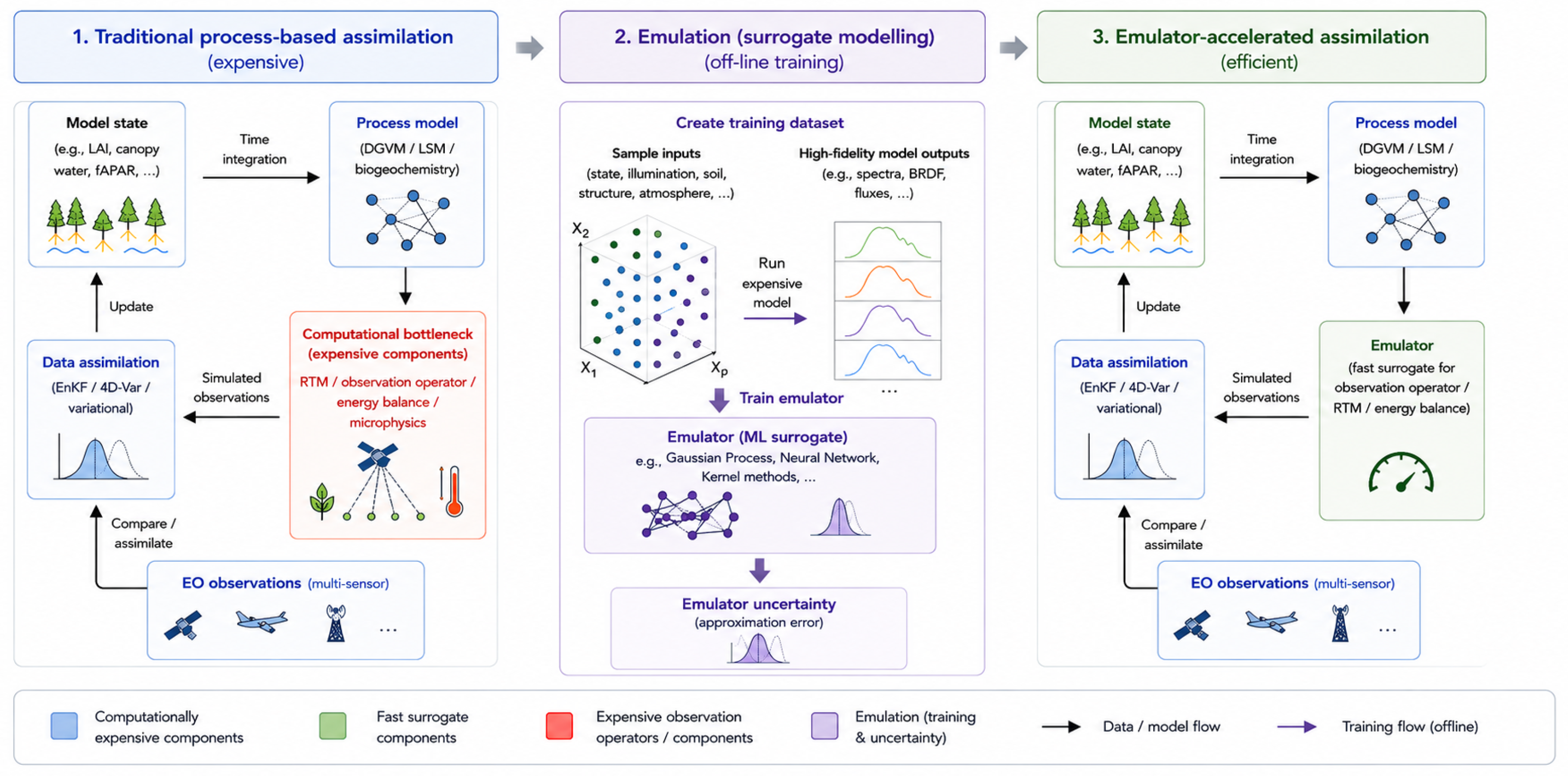
From a system perspective, emulation and surrogate modelling provide a principled pathway to address these challenges in scaling and integrating L4 inference systems. As briefly introduced within the hybrid modelling paradigm (see Section 5), emulation enables computationally expensive components of the estimation chain—such as radiative transfer models, observation operators, or full process-based simulators—to be approximated by data-driven models (e.g., [120,121,131]). Once trained, such emulators can deliver orders-of-magnitude speedups while retaining sufficient accuracy for estimation purposes (see review [119]). In this context, emulation can be interpreted as a concrete mechanism of hybridization, in which data-driven components replace or augment computational bottlenecks within physically based models. This enables tighter coupling between EO data and dynamic models, facilitating iterative estimation, ensemble-based inference, and large-scale deployment while preserving physical interpretability [30]. Figure 8 illustrates this transition from traditional process-based assimilation to emulator-accelerated workflows.

At the same time, emulation introduces additional sources of uncertainty and potential bias. Approximation errors, limited extrapolation capacity, and dependence on the training domain can affect estimation quality. Emulator uncertainty must therefore be explicitly represented and propagated alongside process and observation uncertainty [119,131]. When appropriately validated, emulation enables physically informed L4 inference systems to achieve operational scalability without fundamentally changing the underlying estimation framework, making it a key enabling technology for next-generation EO-based L4 products.

8.2. Three Priorities for Next-Generation Operational L4 Systems

Taken together, these developments shift the focus from standalone products to coherent inference systems. In this context, three key priorities emerge for advancing toward coherent operational L4 systems:

• Operational systems are most effective when they are explicitly scale-aware. This goes beyond handling multi-resolution inputs: observation resolution, retrieval resolution, and model resolution may differ systematically, and effective-scale considerations should therefore be embedded throughout the estimation chain.
• Operational systems are most effective when they are explicitly uncertainty-aware. Point estimates alone are insufficient. Uncertainty should be treated as a first-class output, with traceability to observation errors, model structure, and estimation design.
• Operational systems are most effective when they are hybrid, modular, and emulator-enabled. Purely process-based systems remain difficult to scale globally at high temporal resolution, while purely data-driven systems remain vulnerable to domain shift and limited physical interpretability. Modular hybridization provides a pathway to combine mechanistic consistency with scalability, provided that component interactions remain physically and statistically coherent.

Ultimately, operational L4 systems should be understood as integrated estimation architectures rather than collections of products. Their reliability depends on the consistent integration of observation characteristics, model representations, effective scale, and uncertainty across the complete observation–model inference chain.

8.3. Imaging Spectroscopy and Next-Generation L4 Estimation

Looking ahead, upcoming spaceborne imaging spectroscopy missions, such as the FLuorescence EXplorer (FLEX) [132] and the Copernicus Hyperspectral Imaging Mission (CHIME) [133], are expected to strengthen the observational basis for L4 inference by providing spectrally resolved measurements of vegetation biochemistry, structure, and photosynthetic activity [2,133,134]. In particular, SIF provides a more direct constraint on photosynthetic activity and its variability across ecosystems [2]. These developments create new opportunities for constraining L4 variables, including GPP, ET, and biochemical traits, through improved sensitivity to canopy composition and function. At the same time, they increase the demands placed on inference systems by expanding data volume, spectral dimensionality, and observation-operator complexity.

From an L4 modelling perspective, imaging spectroscopy reinforces the need for physically consistent observation operators. RTMs capable of representing coupled reflectance and SIF signals, such as SCOPE, provide a critical link between observations and ecosystem processes [79,80]. Advanced radiative transfer frameworks extend this capability to heterogeneous and structurally complex canopies. Three-dimensional models such as DART [95] and LESS [96] explicitly represent canopy architecture, illumination geometry, and multiple scattering processes, enabling the simulation of coupled reflectance and SIF signals under realistic scene conditions. These developments highlight that observation operators are not merely forward models, but integral components of the inference system, linking radiative processes, canopy structure, and ecosystem function across scales.

More broadly, imaging spectroscopy strengthens the case for scale-aware, uncertainty-aware, and hybrid estimation architectures in which spectral richness is translated into physically interpretable constraints on latent ecosystem variables. Rather than simply increasing the volume and dimensionality of EO observations, upcoming missions such as FLEX and CHIME reinforce the need for coherent L2–L4 inference systems that jointly address observation physics, scale mismatch, uncertainty propagation, and model consistency across the complete observation–model chain.

9. Conclusions

L4 products derived from EO are inherently model-conditioned estimates of latent ecosystem states, fluxes, and trajectories. Their credibility is not determined by EO data quality alone, but by how the full observation–retrieval–model–estimation chain represents scale, observation physics, and uncertainty.

This review has examined three complementary approaches for L4 estimation: process-based assimilation, ML, and hybrid frameworks, which can be interpreted as explicit, implicit, and integrated inference systems. These approaches provide distinct yet complementary responses to a common inference challenge. Process-based approaches ensure dynamical and physical consistency, but remain computationally demanding and sensitive to structural inadequacy. ML methods offer flexibility and scalability, but are constrained by training-domain dependence, limited extrapolation capacity, and ambiguity in uncertainty interpretation. Hybrid frameworks provide a pathway to balance these trade-offs, provided that interactions between mechanistic and data-driven components remain well controlled. Across all approaches, EO-specific constraints are intrinsic to the inference problem. Scale mismatch, nonlinear observation operators, temporal sampling limitations, and multi-sensor inconsistencies determine the effective information content of EO data and impose fundamental limits on L4 credibility.

Operational L4 products are already established, yet remain fragmented across modelling frameworks, datasets, and processing chains. Progress therefore depends not only on improved algorithms, but on the design of integrated inference frameworks that jointly combine observations, models, and uncertainty, moving beyond isolated products. In such integrated frameworks, scale-awareness and uncertainty-awareness must be embedded throughout the processing chain, from observation and retrieval to estimation and validation. This requires explicit representation of observation operators, consistent treatment of multi-scale information, and transparent propagation of uncertainty across components.

Looking ahead, next-generation L4 systems will likely rely on hybrid, modular, and cloud-native architectures capable of maintaining traceability across sensors, scales, and time. In this context, emulation and surrogate modelling will play an increasingly important role by alleviating computational bottlenecks and enabling scalable, uncertainty-aware inference. Ultimately, a fundamental challenge of L4 estimation lies not only in data availability, but in the design of inference systems consistent with the information content and limitations of EO data. Realizing the full potential of EO for robust, interpretable, and decision-relevant characterization of terrestrial ecosystem functioning requires that observation characteristics, model structure, and uncertainty representation are jointly considered within a coherent inference framework. Addressing this challenge is essential for exploiting next-generation EO missions and advancing a quantitative, uncertainty-aware understanding of the Earth system.

References

1. Verrelst, J.; Camps-Valls, G.; Muñoz-Marí, J.; Rivera, J.P.; Veroustraete, F.; Clevers, J.G.; Moreno, J. Optical remote sensing and the retrieval of terrestrial vegetation bio-geophysical properties—A review. ISPRS J. Photogramm. Remote Sens. 2015, 108, 273–290. [Google Scholar] [CrossRef]
2. Mohammed, G.H.; Colombo, R.; Middleton, E.M.; Rascher, U.; van der Tol, C.; Nedbal, L.; Goulas, Y.; Pérez-Priego, Ó.; Damm, A.; Meroni, M.; et al. Remote sensing of solar-induced chlorophyll fluorescence (SIF) in vegetation: 50 years of progress. Remote Sens. Environ. 2019, 231, 111177. [Google Scholar] [CrossRef] [PubMed]
3. Frankenberg, C.; Butz, A.; Toon, G.C. Disentangling chlorophyll fluorescence from atmospheric scattering effects in O2 A-band spectra of reflected sunlight. Geophys. Res. Lett. 2011, 38, L03801. [Google Scholar] [CrossRef]
4. Sun, Y.; Frankenberg, C.; Jung, M.; Joiner, J.; Guanter, L.; Köhler, P.; Magney, T. Overview of solar-induced chlorophyll fluorescence (SIF) from the Orbiting Carbon Observatory-2: Retrieval, cross-mission comparison, and global monitoring for GPP. Remote Sens. Environ. 2018, 209, 808–823. [Google Scholar] [CrossRef]
5. Zhang, Y.; Joiner, J.; Alemohammad, S.H.; Zhou, S.; Gentine, P. A global spatially contiguous solar-induced fluorescence (CSIF) dataset using neural networks. Biogeosciences 2018, 15, 5779–5800. [Google Scholar] [CrossRef]
6. Joiner, J.; Yoshida, Y.; Vasilkov, A.P.; Middleton, E.M.; Campbell, P.K.E.; Yoshida, Y. The seasonal cycle of satellite chlorophyll fluorescence observations and its relationship to vegetation phenology and ecosystem atmosphere carbon exchange. Remote Sens. Environ. 2014, 152, 375–391. [Google Scholar] [CrossRef]
7. Porcar-Castell, A.; Tyystjärvi, E.; Atherton, J.; Van der Tol, C.; Flexas, J.; Pfündel, E.; Moreno, J.; Frankenberg, C.; Berry, J. Linking chlorophyll a fluorescence to photosynthesis for remote sensing applications: Mechanisms and challenges. J. Exp. Bot. 2014, 65, 4065–4095. [Google Scholar] [CrossRef] [PubMed]
8. Running, S.W.; Nemani, R.R.; Heinsch, F.A.; Zhao, M.; Reeves, M.; Hashimoto, H. A Continuous Satellite-Derived Measure of Global Terrestrial Primary Production. BioScience 2004, 54, 547–560. [Google Scholar] [CrossRef]
9. Beer, C.; Reichstein, M.; Tomelleri, E.; Ciais, P.; Jung, M.; Carvalhais, N.; Rödenbeck, C.; Arain, M.A.; Baldocchi, D.; Bonan, G.B.; et al. Terrestrial Gross Carbon Dioxide Uptake: Global Distribution and Covariation with Climate. Science 2010, 329, 834–838. [Google Scholar] [CrossRef] [PubMed]
10. Yuan, W.; Zheng, Y.; Piao, S.; Ciais, P.; Lombardozzi, D.; Wang, Y.; Ryu, Y.; Chen, G.; Dong, W.; Hu, Z.; et al. Increased atmospheric vapor pressure deficit reduces global vegetation growth. Sci. Adv. 2019, 5, eaax1396. [Google Scholar] [CrossRef] [PubMed]
11. Zhang, L.X.; Zhou, D.C.; Fan, J.W.; Hu, Z.M. Comparison of four light use efficiency models for estimating terrestrial gross primary production. Ecol. Model. 2015, 300, 30–39. [Google Scholar] [CrossRef]
12. Jung, M.; Schwalm, C.; Migliavacca, M.; Walther, S.; Camps-Valls, G.; Koirala, S.; Anthoni, P.; Besnard, S.; Bodesheim, P.; Carvalhais, N.; et al. Scaling carbon fluxes from eddy covariance sites to globe: Synthesis and evaluation of the FLUXCOM approach. Biogeosciences 2020, 17, 1343–1365. [Google Scholar] [CrossRef]
13. Tramontana, G.; Jung, M.; Schwalm, C.R.; Ichii, K.; Camps-Valls, G.; Raduly, B.; Reichstein, M.; Arain, M.A.; Cescatti, A.; Kiely, G.; et al. Predicting carbon dioxide and energy fluxes across global FLUXNET sites with regression algorithms. Biogeosciences 2016, 13, 4291–4313. [Google Scholar] [CrossRef]
14. Nelson, J.A.; Walther, S.; Gans, F.; Kraft, B.; Weber, U.; Novick, K.; Buchmann, N.; Migliavacca, M.; Wohlfahrt, G.; Šigut, L.; et al. X-BASE: The first terrestrial carbon and water flux products from an extended data-driven scaling framework, FLUXCOM-X. Biogeosciences 2024, 21, 5079–5115. [Google Scholar] [CrossRef]
15. Reichle, R.H. Data assimilation methods in the Earth sciences. Adv. Water Resour. 2008, 31, 1411–1418. [Google Scholar] [CrossRef]
16. Reichle, R.H.; Liu, Q.; Koster, R.D.; Crow, W.T.; De Lannoy, G.J.M.; Kimball, J.S.; Ardizzone, J.V.; Bosch, D.; Colliander, A.; Cosh, M.; et al. Version 4 of the SMAP Level-4 Soil Moisture Algorithm and Data Product. J. Adv. Model. Earth Syst. 2019, 11, 3106–3130. [Google Scholar] [CrossRef]
17. Kumar, S.V.; Kolassa, J.; Reichle, R.; Crow, W.; de Lannoy, G.; de Rosnay, P.; MacBean, N.; Girotto, M.; Fox, A.; Quaife, T.; et al. An Agenda for Land Data Assimilation Priorities: Realizing the Promise of Terrestrial Water, Energy, and Vegetation Observations From Space. J. Adv. Model. Earth Syst. 2022, 14, e2022MS003259. [Google Scholar] [CrossRef]
18. Anav, A.; Friedlingstein, P.; Beer, C.; Ciais, P.; Harper, A.; Jones, C.; Murray-Tortarolo, G.; Papale, D.; Parazoo, N.C.; Peylin, P.; et al. Spatiotemporal patterns of terrestrial gross primary production: A review. Rev. Geophys. 2015, 53, 785–818. [Google Scholar] [CrossRef]
19. Sitch, S.; O’Sullivan, M.; Robertson, E.; Friedlingstein, P.; Albergel, C.; Anthoni, P.; Arneth, A.; Arora, V.K.; Bastos, A.; Bastrikov, V.; et al. Trends and Drivers of Terrestrial Sources and Sinks of Carbon Dioxide: An Overview of the TRENDY Project. Glob. Biogeochem. Cycles 2024, 38, e2024GB008102. [Google Scholar] [CrossRef]
20. Piao, S.; Sitch, S.; Ciais, P.; Friedlingstein, P.; Peylin, P.; Wang, X.; Ahlström, A.; Anav, A.; Canadell, J.G.; Cong, N.; et al. Evaluation of terrestrial carbon cycle models for their response to climate variability and to. Glob. Change Biol. 2013, 19, 2117–2132. [Google Scholar] [CrossRef] [PubMed]
21. Knorr, W.; Williams, M.; Thum, T.; Kaminski, T.; Voßbeck, M.; Scholze, M.; Quaife, T.; Smallman, T.L.; Steele-Dunne, S.C.; Vreugdenhil, M.; et al. A comprehensive land-surface vegetation model for multi-stream data assimilation, D&B v1.0. Geosci. Model Dev. 2025, 18, 2137–2159. [Google Scholar] [CrossRef]
22. Wang, Z.; Peñuelas, J.; Tagesson, T.; Smith, W.K.; Wu, M.; He, W.; Sitch, S.; Wang, S. Evolution of Global Terrestrial Gross Primary Productivity Trend. Ecosyst. Health Sustain. 2024, 10, 0278. [Google Scholar] [CrossRef]
23. Zhang, Y.; Ye, A. Uncertainty analysis of multiple terrestrial gross primary productivity products. Glob. Ecol. Biogeogr. 2022, 31, 2204–2218. [Google Scholar] [CrossRef]
24. Evensen, G. Data Assimilation: The Ensemble Kalman Filter; Springer: Berlin/Heidelberg, Germany, 2009. [Google Scholar] [CrossRef]
25. Tarantola, A. Inverse Problem Theory and Methods for Model Parameter Estimation; SIAM: Philadelphia, PA, USA, 2005. [Google Scholar] [CrossRef]
26. Verrelst, J.; Malenovský, Z.; van der Tol, C.; Camps-Valls, G.; Gastellu-Etchegorry, J.P.; Lewis, P.; North, P.; Moreno, J. Quantifying vegetation biophysical variables from imaging spectroscopy data: A review on retrieval methods. Surv. Geophys. 2019, 40, 589–629. [Google Scholar] [CrossRef] [PubMed]
27. Verrelst, J.; Kovács, D.D.; Rivera-Caicedo, J.P. Vegetation Trait Mapping With Optical Remote Sensing: Recent Advances in Methods and Applications. In Comprehensive Remote Sensing; Elsevier: Amsterdam, The Netherlands, 2026. [Google Scholar] [CrossRef]
28. Carrassi, A.; Bocquet, M.; Bertino, L.; Evensen, G. Data assimilation in the geosciences: An overview of methods, issues, and perspectives. WIREs Clim. Change 2018, 9, e535. [Google Scholar] [CrossRef]
29. Reichstein, M.; Camps-Valls, G.; Stevens, B.; Jung, M.; Denzler, J.; Carvalhais, N.; Prabhat, F. Deep learning and process understanding for data-driven Earth system science. Nature 2019, 566, 195–204. [Google Scholar] [CrossRef] [PubMed]
30. Karpatne, A.; Atluri, G.; Faghmous, J.H.; Steinbach, M.; Banerjee, A.; Ganguly, A.R.; Shekhar, S.; Samatova, N.; Kumar, V. Theory-guided data science: A new paradigm for scientific discovery. IEEE Trans. Knowl. Data Eng. 2017, 29, 2318–2331. [Google Scholar] [CrossRef]
31. Willard, J.; Jia, X.; Xu, S.; Steinbach, M.; Kumar, V. Integrating physics-based modeling with machine learning: A survey. ACM Comput. Surv. 2022, 55, 66. [Google Scholar] [CrossRef]
32. Mu, Q.; Zhao, M.; Running, S.W. Improvements to a MODIS global terrestrial evapotranspiration algorithm. Remote Sens. Environ. 2011, 115, 1781–1800. [Google Scholar] [CrossRef]
33. Miralles, D.G.; Bonte, O.; Koppa, A.; Baez-Villanueva, O.M.; Tronquo, E.; Zhong, F.; Beck, H.E.; Hulsman, P.; Dorigo, W.A.; Verhoest, N.E.C.; et al. GLEAM4: Global land evaporation and soil moisture dataset at 0.1° resolution from 1980 to near present. Sci. Data 2025, 12, 416. [Google Scholar] [CrossRef] [PubMed]
34. Santoro, M.; Cartus, O.; Carvalhais, N.; Rozendaal, D.M.A.; Avitabile, V.; Araza, A.; de Bruin, S.; Herold, M.; Quegan, S.; Rodríguez-Veiga, P.; et al. The global forest above-ground biomass pool for 2010 estimated from high-resolution satellite observations. Earth Syst. Sci. Data 2021, 13, 3927–3950. [Google Scholar] [CrossRef]
35. Jung, M.; Reichstein, M.; Schwalm, C.R.; Huntingford, C.; Sitch, S.; Ahlström, A.; Arneth, A.; Camps-Valls, G.; Ciais, P.; Friedlingstein, P. Compensatory water effects link yearly global land CO2 sink changes to temperature. Nature 2017, 541, 516–520. [Google Scholar] [CrossRef] [PubMed]
36. Dwyer, J.L.; Roy, D.P.; Sauer, B.; Jenkerson, C.B.; Zhang, H.K.; Lymburner, L. Analysis ready data: Enabling analysis of the Landsat archive. Remote Sens. 2018, 10, 1363. [Google Scholar] [CrossRef]
37. Ju, J.; Zhou, Q.; Freitag, B.; Roy, D.P.; Zhang, H.K.; Sridhar, M.; Mandel, J.; Arab, S.; Schmidt, G.; Crawford, C.J.; et al. The Harmonized Landsat and Sentinel-2 version 2.0 surface reflectance dataset. Remote Sens. Environ. 2025, 324, 114723. [Google Scholar] [CrossRef]
38. Verrelst, J.; Reyes-Muñoz, A.; Moreno, J.; Camps-Valls, G. Scale-Aware Interpretation of Earth Observation Vegetation Products: Concepts, Challenges, and Future Perspectives. Remote Sens. 2026, 18, 1951. [Google Scholar] [CrossRef]
39. Zhu, S.; Dong, W.; Myrgiotis, V.; Xu, J.; Reyes-Muñoz, P.; Gharun, M.; Ma, R.; Chen, M.; Dash, J. First global carbon dynamics from an observational and process-informed hybrid perspective: Oversimplified respiration representation likely drives divergence in terrestrial carbon sequestration across models. Agric. For. Meteorol. 2026, 385, 111197. [Google Scholar] [CrossRef]
40. Berger, K.; Hostert, P.; Schlerf, M.; Immitzer, M.; Szantoi, Z.; Okujeni, A.; Foerster, S.; Colditz, R.; Giardino, C.; Machwitz, M.; et al. Advancing optical earth observation for EU policies: Needs, opportunities, recommendations. Environ. Sci. Eur. 2026, 38, 52. [Google Scholar] [CrossRef]
41. Wharton, S.W.; Myers, M.F. (Eds.) MTPE/EOS Data Products Handbook, Volume 1: TRMM and AM-1; NASA Goddard Space Flight Center: Greenbelt, MD, USA, 1997.
42. Global Climate Observing System (GCOS). The Global Observing System for Climate: Implementation Plan; GCOS Implementation Plan GCOS-244; World Meteorological Organization (WMO): Geneva, Switzerland, 2022. [Google Scholar]
43. Kandasamy, S.; Baret, F.; Verger, A.; Neveux, P.; Weiss, M. A comparison of methods for smoothing and gap filling time series of remote sensing observations–application to MODIS LAI products. Biogeosciences 2013, 10, 4055–4071. [Google Scholar] [CrossRef]
44. Badgley, G.; Field, C.B.; Berry, J.A. Canopy near-infrared reflectance and terrestrial photosynthesis. Sci. Adv. 2017, 3, e1602244. [Google Scholar] [CrossRef] [PubMed]
45. Fang, H.; Baret, F.; Plummer, S.; Schaepman-Strub, G. An Overview of Global Leaf Area Index (LAI): Methods, Products, Validation, and Applications. Rev. Geophys. 2019, 57, 739–799. [Google Scholar] [CrossRef]
46. Reyes-Muñoz, P.; Kovács, D.D.; Berger, K.; Pipia, L.; Belda, S.; Rivera-Caicedo, J.P.; Verrelst, J. Inferring global terrestrial carbon fluxes from the synergy of Sentinel 3 & 5P with Gaussian process hybrid models. Remote Sens. Environ. 2024, 305, 114072. [Google Scholar] [CrossRef]
47. Jung, M.; Koirala, S.; Weber, U.; Ichii, K.; Gans, F.; Camps-Valls, G.; Papale, D.; Schwalm, C.; Tramontana, G.; Reichstein, M. The FLUXCOM ensemble of global land-atmosphere energy fluxes. Sci. Data 2019, 6, 74. [Google Scholar] [CrossRef] [PubMed]
48. Saatchi, S.S.; Harris, N.L.; Brown, S.; Lefsky, M.; Mitchard, E.T.A.; Salas, W.; Zutta, B.R.; Buermann, W.; Lewis, S.L.; Hagen, S.; et al. Benchmark map of forest carbon stocks in tropical regions across three continents. Proc. Natl. Acad. Sci. USA 2011, 108, 9899–9904. [Google Scholar] [CrossRef] [PubMed]
49. Baccini, A.; Goetz, S.J.; Walker, W.S.; Laporte, N.T.; Sun, M.; Sulla-Menashe, D.; Hackler, J.; Beck, P.S.A.; Dubayah, R.; Friedl, M.A.; et al. Estimated carbon dioxide emissions from tropical deforestation improved by carbon-density maps. Nat. Clim. Change 2012, 2, 182–185. [Google Scholar] [CrossRef]
50. Tian, L.; Wang, X.; Tang, Y.; Qian, C.; Liu, L.; Fu, W.; Liu, M. Review of Remote Sensing-Based Methods for Forest Aboveground Biomass Estimation: Progress, Challenges, and Prospects. Forests 2023, 14, 1086. [Google Scholar] [CrossRef]
51. Lobell, D.B.; Thau, D.; Seifert, C.; Engle, E.; Little, B. A scalable satellite-based crop yield mapper. Remote Sens. Environ. 2015, 164, 324–333. [Google Scholar] [CrossRef]
52. Jeong, J.H.; Resop, J.P.; Mueller, N.D.; Fleisher, D.H.; Yun, K.S.; Butler, E.E.; Timlin, D.J.; Shim, K.M.; Gerber, J.S.; Reddy, V.R. Random forests for global and regional crop yield predictions. PLoS ONE 2016, 11, e0156571. [Google Scholar] [CrossRef] [PubMed]
53. van Klompenburg, T.; Kassahun, A.; Catal, C. Crop yield prediction using machine learning: A systematic literature review. Comput. Electron. Agric. 2020, 177, 105709. [Google Scholar] [CrossRef]
54. Meghraoui, K.; Sebari, I.; Pilz, J.; Ait El Kadi, K.; Bensiali, S. Applied Deep Learning-Based Crop Yield Prediction. Technologies 2024, 12, 43. [Google Scholar] [CrossRef]
55. Reichle, R.H.; De Lannoy, G.J.M.; Koster, R.D.; Crow, W.T.; Kimball, J.S. Assessment of the SMAP Level-4 Surface and Root-Zone Soil Moisture Product Using In Situ Measurements. J. Hydrometeorol. 2017, 18, 2621–2645. [Google Scholar] [CrossRef]
56. Reichle, R.H.; Liu, Q.; Ardizzone, J.V.; Crow, W.T.; De Lannoy, G.J.M.; Kimball, J.S.; Koster, R.D. IMERG Precipitation Improves the SMAP Level-4 Soil Moisture Product. J. Hydrometeorol. 2023, 24, 1699–1723. [Google Scholar] [CrossRef]
57. Sitch, S.; Friedlingstein, P.; Gruber, N.; Jones, S.D.; Murray-Tortarolo, G.; Ahlström, A.; Doney, S.C.; Graven, H.; Heinze, C.; Huntingford, C.; et al. Recent trends and drivers of regional sources and sinks of carbon dioxide. Biogeosciences 2015, 12, 653–679. [Google Scholar] [CrossRef]
58. Rayner, P.J.; Scholze, M.; Knorr, W.; Kaminski, T.; Giering, R.; Widmann, H. Two decades of terrestrial carbon fluxes from a carbon cycle data assimilation system (CCDAS). Glob. Biogeochem. Cycles 2005, 19, GB2026. [Google Scholar] [CrossRef]
59. Byrne, B.; Liu, J.; Bloom, A.A.; Bowman, K.W.; Butterfield, Z.; Chevallier, F.; Crowell, S.M.R.; Eldering, A.; Jacobson, A.R.; Jones, D.B.A.; et al. National CO2 budgets (2015–2020) inferred from atmospheric CO2 observations in support of the global stocktake. Earth Syst. Sci. Data 2023, 15, 963–1004. [Google Scholar] [CrossRef]
60. Jönsson, P.; Eklundh, L. TIMESAT—A program for analyzing time-series of satellite sensor data. Comput. Geosci. 2004, 30, 833–845. [Google Scholar] [CrossRef]
61. Verbesselt, J.; Hyndman, R.; Zeileis, A.; Culvenor, D. Phenological change detection while accounting for abrupt and gradual trends in satellite image time series. Remote Sens. Environ. 2010, 114, 2970–2980. [Google Scholar] [CrossRef]
62. Belda, S.; Pipia, L.; Morcillo-Pallarés, P.; Rivera-Caicedo, J.P.; Amin, E.; De Grave, C.; Verrelst, J. DATimeS: A machine learning time series GUI toolbox for gap-filling and vegetation phenology trends detection. Environ. Model. Softw. 2020, 127, 104666. [Google Scholar] [CrossRef] [PubMed]
63. Li, X.; Liu, F.; Ma, C.; Hou, J.; Zheng, D.; Ma, H.; Bai, Y.; Han, X.; Vereecken, H.; Yang, K.; et al. Land Data Assimilation: Harmonizing Theory and Data in Land Surface Process Studies. Rev. Geophys. 2024, 62, e2022RG000801. [Google Scholar] [CrossRef]
64. Lewis, P.; Gómez-Dans, J.; Kaminski, T.; Settle, J.; Quaife, T.; Gobron, N.; Styles, J.; Berger, M. An earth observation land data assimilation system (EO-LDAS). Remote Sens. Environ. 2012, 120, 219–235. [Google Scholar] [CrossRef]
65. Bannister, R.N. A review of operational methods of variational and ensemble-variational data assimilation. Q. J. R. Meteorol. Soc. 2017, 143, 607–633. [Google Scholar] [CrossRef]
66. De Lannoy, G.J.M.; Reichle, R.H.; Liu, Q. Assimilation of SMOS brightness temperatures or soil moisture retrievals into a land surface model. Remote Sens. Environ. 2016, 180, 292–304. [Google Scholar] [CrossRef]
67. Knorr, W.; Kaminski, T.; Scholze, M.; Gobron, N.; Pinty, B.; Giering, R.; Mathieu, P.P. Carbon cycle data assimilation with a generic phenology model. J. Geophys. Res. Biogeosci. 2010, 115, G04017. [Google Scholar] [CrossRef]
68. Kaminski, T.; Knorr, W.; Scholze, M.; Gobron, N.; Pinty, B.; Giering, R.; Mathieu, P.P. Consistent assimilation of MERIS FAPAR and atmospheric CO2 into a terrestrial vegetation model and interactive mission benefit analysis. Biogeosciences 2012, 9, 3173–3184. [Google Scholar] [CrossRef]
69. Scholze, M.; Buchwitz, M.; Dorigo, W.A.; Guanter, L.; Quegan, S. Reviews and syntheses: Systematic Earth observations for use in terrestrial carbon cycle data assimilation systems. Biogeosciences 2017, 14, 3401–3429. [Google Scholar] [CrossRef]
70. Krinner, G.; Viovy, N.; de Noblet-Ducoudré, N.; Ogée, J.; Polcher, J.; Friedlingstein, P.; Ciais, P.; Sitch, S.; Prentice, I.C. A dynamic global vegetation model for studies of the coupled atmosphere-biosphere system. Glob. Biogeochem. Cycles 2005, 19, GB1015. [Google Scholar] [CrossRef]
71. Clark, D.; Mercado, L.; Sitch, S.; Jones, C.; Gedney, N.; Best, M.; Pryor, M.; Rooney, G.; Essery, R.; Blyth, E.; et al. The Joint UK Land Environment Simulator (JULES), model description–Part 2: Carbon fluxes and vegetation dynamics. Geosci. Model Dev. 2011, 4, 701–722. [Google Scholar] [CrossRef]
72. Lawrence, D.M.; Fisher, R.A.; Koven, C.D.; Oleson, K.W.; Swenson, S.C.; Bonan, G.; Collier, N.; Ghimire, B.; Van Kampenhout, L.; Kennedy, D.; et al. The Community Land Model version 5: Description of new features, benchmarking, and impact of forcing uncertainty. J. Adv. Model. Earth Syst. 2019, 11, 4245–4287. [Google Scholar] [CrossRef]
73. Peylin, P.; Bacour, C.; MacBean, N.; Leonard, S.; Rayner, P.J.; Koffi, E.N.; Scholze, M.; Kaminski, T.; Kato, T.; Chevallier, F. Global atmospheric carbon budget: Results from an ensemble of atmospheric. Biogeosciences 2013, 10, 6699–6720. [Google Scholar] [CrossRef]
74. Williams, M.; Schwarz, P.A.; Law, B.E.; Irvine, J.; Kurpius, M.R. An improved analysis of forest carbon dynamics using data assimilation. Glob. Change Biol. 2005, 11, 89–105. [Google Scholar] [CrossRef]
75. Knorr, W.; Heimann, M. Uncertainties in global terrestrial biosphere modeling: 1. A comprehensive sensitivity analysis with a new photosynthesis and energy balance scheme. Glob. Biogeochem. Cycles 2001, 15, 207–225. [Google Scholar] [CrossRef]
76. Huang, J.; Gómez-Dans, J.L.; Huang, H.; Ma, H.; Wu, Q.; Lewis, P.E.; Liang, S.; Chen, Z.; Xue, J.H.; Wu, Y.; et al. Assimilation of remote sensing into crop growth models: Current status and perspectives. Agric. For. Meteorol. 2019, 276, 107609. [Google Scholar] [CrossRef]
77. Wang, J.; Wang, Y.; Qi, Z. Remote sensing data assimilation in crop growth modeling from an agricultural perspective: New insights on challenges and prospects. Agronomy 2024, 14, 1920. [Google Scholar] [CrossRef]
78. Jacquemoud, S.; Verhoef, W.; Baret, F.; Bacour, C.; Zarco-Tejada, P.J.; Asner, G.P.; François, C.; Ustin, S.L. PROSPECT + SAIL models: A review of use for vegetation characterization. Remote Sens. Environ. 2009, 113, S56–S66. [Google Scholar] [CrossRef]
79. van der Tol, C.; Verhoef, W.; Timmermans, J.; Verhoef, A.; Su, Z. An integrated model of soil-canopy spectral radiances, photosynthesis, fluorescence, temperature and energy balance. Biogeosciences 2009, 6, 3109–3129. [Google Scholar] [CrossRef]
80. Yang, P.; Prikaziuk, E.; Verhoef, W.; van der Tol, C. SCOPE 2.0: A model to simulate vegetated land surface fluxes and satellite signals. Geosci. Model Dev. 2021, 14, 4697–4712. [Google Scholar] [CrossRef]
81. Pinty, B.; Lavergne, T.; Dickinson, R.E.; Widlowski, J.; Gobron, N.; Verstraete, M.M. Simplifying the interaction of land surfaces with radiation for relating remote sensing products to climate models. J. Geophys. Res. Atmos. 2006, 111, D02116. [Google Scholar] [CrossRef]
82. Li, B.; Ryu, Y.; Jiang, C.; Dechant, B.; Liu, J.; Yan, Y.; Li, X. BESSv2.0: A satellite-based and coupled-process model for quantifying long-term global land–atmosphere fluxes. Remote Sens. Environ. 2023, 295, 113696. [Google Scholar] [CrossRef]
83. Smith, B.; Prentice, I.C.; Sykes, M.T. Representation of vegetation dynamics in the modelling of terrestrial ecosystems: Comparing two contrasting approaches within European climate space. Glob. Ecol. Biogeogr. 2001, 10, 621–637. [Google Scholar] [CrossRef]
84. Sitch, S.; Smith, B.; Prentice, I.C.; Arneth, A.; Bondeau, A.; Cramer, W.; Kaplan, J.O.; Levis, S.; Lucht, W.; Sykes, M.T.; et al. Evaluation of ecosystem dynamics, plant geography and terrestrial carbon cycling in the LPJ dynamic global vegetation model. Glob. Change Biol. 2003, 9, 161–185. [Google Scholar] [CrossRef]
85. Jones, J.W.; Hoogenboom, G.; Porter, C.H.; Boote, K.J.; Batchelor, W.D.; Hunt, L.A.; Wilkens, P.W.; Singh, U.; Gijsman, A.J.; Ritchie, J.T. The DSSAT cropping system model. Eur. J. Agron. 2003, 18, 235–265. [Google Scholar] [CrossRef]
86. Keating, B.A.; Carberry, P.S.; Hammer, G.L.; Probert, M.E.; Robertson, M.J.; Holzworth, D.; Huth, N.I.; Hargreaves, J.N.G.; Meinke, H.; Hochman, Z.; et al. An overview of APSIM, a model designed for farming systems simulation. Eur. J. Agron. 2003, 18, 267–288. [Google Scholar] [CrossRef]
87. van Diepen, C.A.; Wolf, J.; van Keulen, H.; Rappoldt, C. WOFOST: A simulation model of crop production. Soil Use Manag. 1989, 5, 16–24. [Google Scholar] [CrossRef]
88. Steduto, P.; Hsiao, T.C.; Fereres, E.; Raes, D. AquaCrop—The FAO crop model to simulate yield response to water: I. Concepts and underlying principles. Agron. J. 2009, 101, 426–437. [Google Scholar] [CrossRef]
89. de Wit, A.; Boogaard, H.; Fumagalli, D.; Janssen, S.; Knapen, R.; van Kraalingen, D.; Supit, I.; van der Wijngaart, R.; van Diepen, K. 25 years of the WOFOST cropping systems model. Agric. Syst. 2019, 168, 154–167. [Google Scholar] [CrossRef]
90. Liang, X.; Lettenmaier, D.P.; Wood, E.F.; Burges, S.J. A simple hydrologically based model of land surface water and energy fluxes for general circulation models. J. Geophys. Res. Atmos. 1994, 99, 14415–14428. [Google Scholar] [CrossRef]
91. Van Beek, L.; Wada, Y.; Bierkens, M.F. Global monthly water stress: 1. Water balance and water availability. Water Resour. Res. 2011, 47, W07517. [Google Scholar] [CrossRef]
92. Bierkens, M.F.P. Global hydrology 2015: State, trends, and directions. Water Resour. Res. 2015, 51, 4923–4947. [Google Scholar] [CrossRef]
93. Bastiaanssen, W.G.M.; Menenti, M.; Feddes, R.A.; Holtslag, A.A.M. A remote sensing surface energy balance algorithm for land (SEBAL): 1. Formulation. J. Hydrol. 1998, 212–213, 198–212. [Google Scholar] [CrossRef]
94. Norman, J.M.; Kustas, W.P.; Humes, K.S. Source approach for estimating soil and vegetation energy fluxes in observations of directional radiometric surface temperature. Agric. For. Meteorol. 1995, 77, 263–293. [Google Scholar] [CrossRef]
95. Gastellu-Etchegorry, J.P.; Martin, E.; Gascon, F. DART: A 3D model for simulating satellite images and studying surface radiation budget. Int. J. Remote Sens. 2004, 25, 73–96. [Google Scholar] [CrossRef]
96. Qi, J.; Xie, D.; Yin, T.; Yan, G.; Gastellu-Etchegorry, J.P.; Li, L.; Zhang, W.; Mu, X.; Norford, L.K. LESS: LargE-Scale remote sensing data and image simulation framework over heterogeneous 3D scenes. Remote Sens. Environ. 2019, 221, 695–706. [Google Scholar] [CrossRef]
97. Verrelst, J.; García-Soria, J.L.; Reyes-Muñoz, P.; De Clerck, E.; Morata, M.; Rivera-Caicedo, J.P. Epistemic and aleatoric uncertainty in optical vegetation trait retrieval: Concepts, Methods, and Outlook. ISPRS J. Photogramm. Remote Sens. 2026, 234, 20–45. [Google Scholar] [CrossRef]
98. Bojinski, S.; Verstraete, M.; Peterson, T.C.; Richter, C.; Simmons, A.; Zemp, M. The concept of Essential Climate Variables in support of climate research, applications, and policy. Bull. Am. Meteorol. Soc. 2014, 95, 1431–1443. [Google Scholar] [CrossRef]
99. Cheng, S.; Quilodrán-Casas, C.; Ouala, S.; Farchi, A.; Liu, C.; Tandeo, P.; Fablet, R.; Lucor, D.; Iooss, B.; Brajard, J.; et al. Machine Learning with Data Assimilation and Uncertainty Quantification for Dynamical Systems: A Review. IEEE/CAA J. Autom. Sin. 2023, 10, 1361–1387. [Google Scholar] [CrossRef]
100. Lorenc, A.C. Analysis methods for numerical weather prediction. Q. J. R. Meteorol. Soc. 1986, 112, 1177–1194. [Google Scholar] [CrossRef]
101. Evensen, G. The Ensemble Kalman Filter: Theoretical formulation and practical implementation. Ocean Dyn. 2003, 53, 343–367. [Google Scholar] [CrossRef]
102. van Leeuwen, P.J. Particle Filtering in Geophysical Systems. Mon. Weather Rev. 2009, 137, 4089–4114. [Google Scholar] [CrossRef]
103. Hamill, T.M.; Snyder, C. A Hybrid Ensemble Kalman Filter–3D Variational Analysis Scheme. Mon. Weather Rev. 2000, 128, 2905–2919. [Google Scholar]
104. Wang, X.; Snyder, C.; Hamill, T.M. On the Theoretical Equivalence of Differently Proposed Ensemble–3DVAR Hybrid Analysis Schemes. Mon. Weather Rev. 2007, 135, 222–227. [Google Scholar] [CrossRef]
105. Emerick, A.A.; Reynolds, A.C. Ensemble smoother with multiple data assimilation. Comput. Geosci. 2013, 55, 3–15. [Google Scholar] [CrossRef]
106. Camps-Valls, G.; Tuia, D.; Zhu, X.X.; Reichstein, M. Deep Learning for the Earth Sciences: A Comprehensive Approach to Remote Sensing, Climate Science and Geosciences; John Wiley & Sons: Hoboken, NJ, USA, 2021. [Google Scholar]
107. Rolnick, D.; Donti, P.L.; Kaack, L.H.; Kochanski, K.; Lacoste, A.; Ross, A.S.; Milojevic-Dupont, N.; Jaques, N.; Waldman-Brown, A.; Luccioni, A.S.; et al. Tackling Climate Change with Machine Learning. ACM Comput. Surv. 2022, 55, 42:1–42:96. [Google Scholar] [CrossRef]
108. Reyes-Muñoz, P.; DKovács, D.; Verrelst, J. Tower-to-global upscaling of terrestrial carbon fluxes driven by MODIS-LAI, Sentinel-3-LAI and ERA5-Land data. Ecol. Indic. 2025, 177, 113597. [Google Scholar] [CrossRef] [PubMed]
109. Zhu, S.; Quaife, T.; Hill, T. Uniform upscaling techniques for eddy covariance FLUXes (UFLUX). Int. J. Remote Sens. 2024, 45, 1450–1476. [Google Scholar] [CrossRef]
110. Zhu, S.; Xu, J.; Zeng, J.; Bao, S.; Chen, Y.; Shi, S.; Zheng, Z.; Dong, W.; Wang, Y.; Shi, J. The UFLUX ensemble of multiple-scale carbon, water, and energy fluxes. Sci. Data 2025, 13, 90. [Google Scholar] [CrossRef] [PubMed]
111. Jabed, M.A.; Murad, M.A.A. Crop yield prediction in agriculture: A comprehensive review of machine learning and deep learning approaches, with insights for future research and sustainability. Heliyon 2024, 10, e40836. [Google Scholar] [CrossRef] [PubMed]
112. Lakshminarayanan, B.; Pritzel, A.; Blundell, C. Simple and scalable predictive uncertainty estimation using deep ensembles. In Proceedings of the Advances in Neural Information Processing Systems, Long Beach, CA, USA, 4–9 December 2017; Volume 30. [Google Scholar]
113. García-Soria, J.L.; Morata, M.; Berger, K.; Pascual-Venteo, A.B.; Rivera-Caicedo, J.P.; Verrelst, J. Evaluating epistemic uncertainty estimation strategies in vegetation trait retrieval using hybrid models and imaging spectroscopy data. Remote Sens. Environ. 2024, 310, 114228. [Google Scholar] [CrossRef]
114. Zeng, J.; Matsunaga, T.; Tan, Z.H.; Saigusa, N.; Shirai, T.; Tang, Y.; Peng, S. Global terrestrial carbon fluxes of 1999–2019 estimated by upscaling eddy covariance data with a random forest. Sci. Data 2020, 7, 313. [Google Scholar] [CrossRef] [PubMed]
115. De Clerck, E.; Reyes-Muñoz, P.; Prikaziuk, E.; Kovács, D.D.; Verrelst, J. High-spatial-resolution gross primary production estimation from Sentinel-2 reflectance using hybrid Gaussian processes modeling. ISPRS J. Photogramm. Remote Sens. 2026, 232, 172–195. [Google Scholar] [CrossRef]
116. Kaul, M.; Hill, R.L.; Walthall, C. Artificial neural networks for corn and soybean yield prediction. Agric. Syst. 2005, 85, 1–18. [Google Scholar] [CrossRef]
117. Jung, M.; Reichstein, M.; Margolis, H.A.; Cescatti, A.; Richardson, A.D.; Arain, A.; Arneth, A.; Bernhofer, C.; Bonal, D.; Chen, J.; et al. Towards global empirical upscaling of FLUXNET eddy covariance observations: Validation of a model tree ensemble approach using a biosphere model. Biogeosciences 2009, 6, 2001–2013. [Google Scholar] [CrossRef]
118. Muruganantham, P.; Wibowo, S.; Grandhi, S.; Samrat, N.H.; Islam, N. A Systematic Literature Review on Crop Yield Prediction with Deep Learning and Remote Sensing. Remote Sens. 2022, 14, 1990. [Google Scholar] [CrossRef]
119. Verrelst, J.; Morata, M.; García-Soria, J.L.; Sun, Y.; Qi, J.; Rivera-Caicedo, J.P. RTM Surrogate Modeling in Optical Remote Sensing: A Review of Emulation for Vegetation and Atmosphere Applications. Remote Sens. 2025, 17, 3618. [Google Scholar] [CrossRef]
120. Rivera, J.P.; Verrelst, J.; Gómez-Dans, J.; Muñoz-Marí, J.; Moreno, J.; Camps-Valls, G. An emulator toolbox to approximate radiative transfer models. Remote Sens. 2015, 7, 9347–9370. [Google Scholar] [CrossRef]
121. Vicent, J.; Verrelst, J.; Rivera-Caicedo, J.P.; Sabater, N.; Munoz-Mari, J.; Camps-Valls, G.; Moreno, J. Emulation as an accurate alternative to interpolation in sampling radiative transfer codes. IEEE J. Sel. Top. Appl. Earth Obs. Remote Sens. 2018, 11, 4918–4931. [Google Scholar] [CrossRef] [PubMed]
122. Woodcock, C.E.; Strahler, A.H. The factor of scale in remote sensing. Remote Sens. Environ. 1987, 21, 311–332. [Google Scholar] [CrossRef]
123. Wu, H.; Li, Z. Scale Issues in Remote Sensing: A Review on Analysis, Processing and Modeling. Sensors 2009, 9, 1768–1793. [Google Scholar] [CrossRef] [PubMed]
124. Belda, S.; Pipia, L.; Verrelst, J. Trends in Satellite Time Series Processing for Vegetation Phenology Monitoring. In Multitemporal Earth Observation Image Analysis; John Wiley & Sons, Ltd.: Hoboken, NJ, USA, 2024; pp. 151–183. [Google Scholar] [CrossRef]
125. Claverie, M.; Ju, J.; Masek, J.G.; Dungan, J.L.; Vermote, E.F.; Roger, J.; Skakun, S.V.; Justice, C. The Harmonized Landsat and Sentinel-2 surface reflectance data set. Remote Sens. Environ. 2018, 219, 145–161. [Google Scholar] [CrossRef]
126. Schramm, M.; Pebesma, E.; Milenković, M.; Foresta, L.; Dries, J.; Jacob, A.; Wagner, W.; Mohr, M.; Neteler, M.; Kadunc, M.; et al. The openeo api–harmonising the use of earth observation cloud services using virtual data cube functionalities. Remote Sens. 2021, 13, 1125. [Google Scholar] [CrossRef]
127. van der Velde, M.; Van Diepen, C.; Baruth, B. The European crop monitoring and yield forecasting system: Celebrating 25 years of JRC MARS Bulletins. Agric. Syst. 2019, 168, 56–57. [Google Scholar] [CrossRef]
128. Verrelst, J.; De Clerck, E.; Verma, B.; Mishra, K.; Caballero, G. Cloud-Native Earth Observation for Quantitative Vegetation Science: Architectures, Workflows, and Scientific Implications. Remote Sens. 2026, 18, 1154. [Google Scholar] [CrossRef]
129. Friedlingstein, P.; O’Sullivan, M.; Jones, M.W.; Andrew, R.M.; Bakker, D.C.E.; Hauck, J.; Landschützer, P.; Le Quéré, C.; Luijkx, I.T.; Peters, G.P.; et al. Global Carbon Budget 2023. Earth Syst. Sci. Data 2023, 15, 5301–5369. [Google Scholar] [CrossRef]
130. Endsley, K.A.; Zhao, M.; Kimball, J.S.; Devadiga, S. Continuity of Global MODIS Terrestrial Primary Productivity Estimates in the VIIRS Era Using Model-Data Fusion. J. Geophys. Res. Biogeosci. 2023, 128, e2023JG007457. [Google Scholar] [CrossRef]
131. Razavi, S.; Tolson, B.A.; Burn, D.H. Review of surrogate modeling in water resources. Water Resour. Res. 2012, 48, W07401. [Google Scholar] [CrossRef]
132. Coppo, P.; Taiti, A.; Pettinato, L.; Francois, M.; Taccola, M.; Drusch, M. Fluorescence imaging spectrometer (FLORIS) for ESA FLEX mission. Remote Sens. 2017, 9, 649. [Google Scholar] [CrossRef]
133. Nieke, J.; Despoisse, L.; Gabriele, A.; Weber, H.; Strese, H.; Ghasemi, N.; Gascon, F.; Alonso, K.; Boccia, V.; Tsonevska, B.; et al. The Copernicus Hyperspectral Imaging Mission for the Environment (CHIME): An Overview of Its Mission, System and Planning Status. In Proceedings of the Sensors, Systems, and Next-Generation Satellites XXVII, Proceedings of SPIE, Amsterdam, The Netherlands, 3–5 September 2023. [Google Scholar] [CrossRef]
134. Drusch, M.; Moreno, J.; Del Bello, U.; Franco, R.; Goulas, Y.; Huth, A.; Kraft, S.; Middleton, E.M.; Miglietta, F.; Mohammed, G.; et al. The fluorescence explorer mission concept—ESA’s earth explorer 8. IEEE Trans. Geosci. Remote Sens. 2016, 55, 1273–1284. [Google Scholar] [CrossRef]
Figure 1. Conceptual framework linking EO data streams to L4 inference. The relationship between the four EO product levels is summarized in Table 1. Satellite radiances are transformed into geophysical variables through retrieval (L2) and subsequently aggregated into consistent spatiotemporal products (L3), both of which remain observation-driven. L4 products are obtained through model-conditioned inference, in which latent ecosystem states and fluxes are estimated using process-based (explicit), ML (implicit), or hybrid (integrated) approaches. The figure highlights the transition from observation-driven EO products to model-conditioned inference systems.
Remotesensing 18 02371 g001
Figure 2. Conceptual comparison of the three main approaches for EO-based L4 inference. Process-based approaches represent ecosystem dynamics explicitly through mechanistic models, often combined with data assimilation. ML methods infer target variables from statistical relationships learned from EO and ancillary data, whereas hybrid frameworks combine process-based and data-driven components within a common inference framework.
Remotesensing 18 02371 g002
Figure 3. Forward and inverse formulations of EO-based L4 inference. In the forward (generative) view, latent ecosystem states and parameters evolve through model dynamics and are mapped to EO data via the observation operator. In the inverse (inference) view, EO data are combined with prior assumptions to estimate posterior states, fluxes, or parameters using process-based, ML, or hybrid inference systems.
Remotesensing 18 02371 g003
Figure 4. Conceptual overview of hybrid modelling strategies for EO-based L4 inference. Representative hybrid modelling strategies include: (A) residual learning, where ML corrects process-model outputs; (B) physics-guided ML, where physical constraints are explicitly embedded within the learning process; (C) tightly coupled hybrid systems, where data-driven components are integrated within dynamic or data assimilation frameworks; (D) simulation-informed ML, where statistical models are trained on synthetic data generated by radiative transfer and/or process-based models; and (E) emulation (surrogate modelling), where ML approximates computationally expensive forward models or observation operators.
Remotesensing 18 02371 g004
Figure 5. Conceptual illustration of how EO constraints shape L4 inference in vegetation monitoring. Multi-sensor EO data provide complementary but heterogeneous information across spatial, temporal, and spectral domains. This information is reduced and distorted by a series of constraints, including scale mismatch, temporal sampling gaps, nonlinear observation operators, retrieval uncertainty, and multi-sensor inconsistencies. These constraints determine the effective information available for inference. The L4 inference system integrates EO data with process-based models, ML, or Hybrid frameworks, optionally supported by emulation. Uncertainty propagation reflects both observation-driven and model-driven sources. The resulting L4 outputs represent model-conditioned estimates of latent ecosystem states and fluxes.
Remotesensing 18 02371 g005
Figure 6. Uncertainty sources and propagation across the EO processing chain from L1 to L4 inference. (A) illustrates how uncertainty originates at the sensor level (L1), propagates through retrieval (L2) and aggregation (L3), and is transformed within L4 inference systems into model-dependent uncertainty components. (B) compares how uncertainty is represented within process-based, ML, and hybrid inference approaches. Together, the figure emphasizes that L4 uncertainty reflects both observation-driven and model-driven contributions.
Remotesensing 18 02371 g006
Figure 7. Comparative synthesis of modelling paradigms for EO-based L4 inference. Process-based (explicit), ML (implicit), and hybrid (integrated) approaches are compared across key dimensions, including dynamical consistency, interpretability, scalability, generalization, uncertainty representation, and sensitivity to EO constraints. The figure summarizes the principal trade-offs among the three approaches and the influence of EO constraints, including scale mismatch, temporal sampling, and observation-operator limitations, on L4 inference.
Remotesensing 18 02371 g007
Figure 8. Conceptual workflow illustrating the use of emulation for scalable L4 EO inference systems. Traditional process-based data assimilation relies on computationally expensive model components that must be evaluated repeatedly. Emulation replaces selected components with surrogate models trained on high-fidelity simulations, enabling computationally efficient inference. The figure depicts the transition from conventional assimilation to emulator-accelerated workflows, while highlighting that emulator uncertainty should be propagated alongside process and observation uncertainties.
Remotesensing 18 02371 g008