A Remote Sensing-Based Groundwater Level Monitoring System Using Machine Learning

Highlights

What are the main findings?

• A remote sensing-based groundwater level monitoring system was proposed and evaluated against in situ observations across the CONUS.
• The Ensemble model adopted by the system significantly outperforms the individual machine learning algorithms (KNN, RF, XGBoost) in reconstructing groundwater levels.

What are the implications of the main findings?

• The proposed GWL monitoring system offers an alternative remote sensing-based approach for groundwater monitoring when in situ measurements are unavailable.
• The Ensemble strategy further enhances model robustness and can thus provide a more reliable and consistent solution for large-scale groundwater monitoring.

Abstract

Groundwater is an essential natural resource for human societies and ecosystems. Traditional groundwater monitoring relies on in situ wells, which are susceptible to discontinuity, influencing water resource management. To overcome this deficiency, this study proposes a remote sensing-based groundwater level (GWL) monitoring system that uses machine learning (ML) algorithms and remotely sensed hydrological parameters to reconstruct well-specific GWL time series. Four machine learning algorithms, including K-Nearest Neighbor (KNN), Random Forest (RF), Extreme Gradient Boosting (XGBoost), and a weight-mean Ensemble strategy, were adopted to construct the models at each well individually for monitoring GWL. Specifically, the GWL data for ~770 wells across the conterminous United States (CONUS) were modeled using remotely sensed precipitation (P), evapotranspiration (ET), terrestrial water storage anomaly (TWSA), and soil moisture (SM) datasets during the period from 2004 to 2019. Afterwards, the performances of models were evaluated during an independent period from 2020 to 2023. The results show that the Ensemble model outperforms the individual baseline models evaluated in this study (i.e., KNN, RF, and XGBoost), achieving a mean coefficient of determination (R²) of 0.81, root mean square error (RMSE) of 0.34 m, normalized RMSE (NRMSE) of 11.8%, and Nash–Sutcliffe efficiency (NSE) of 0.78. The results demonstrate that the proposed system can effectively reconstruct GWL dynamics for most wells. This can be a compensation for missing records for hydrologically significant wells, which are those with historical groundwater observations.

1. Introduction

Groundwater represents the largest distributed store of liquid freshwater on Earth and plays a fundamental role in sustaining human societies and ecosystems [1]. It not only provides essential drinking water for billions of people [2] but also supports a significant part of the world’s irrigated agriculture [3]. Moreover, it sustains the base flows in rivers and wetlands, especially in arid and semi-arid regions where it is often the only perennial water source [4]. However, this vital resource is suffering from widespread overextraction [5] and increasing loss due to climate variability [6], which drives aquifer depletion and quality degradation. Therefore, achieving accurate and continuous monitoring of groundwater is indispensable for sustainable governance [7].

The conventional technique for acquiring accurate groundwater monitoring data remains the use of monitoring wells [8]. These in situ measurements from piezometers are considered the anchor for groundwater assessment and provide direct, high-fidelity records at specific locations. However, monitoring networks face multiple structural challenges. The distribution of monitoring wells is often spatially sparse and uneven [9]. More critically, well records frequently exhibit temporal discontinuities due to instrument failure, maintenance gaps, or the finite operational lifespan of monitoring networks [10]. Although technological innovations such as low-cost MEMS-based sensors and IoT-enabled systems [11] and citizen science initiatives [12] have been produced to enhance data acquisition, the operational continuity of long-term monitoring networks remains vulnerable. Interruptions in well records can compromise long-term trend detection, drought assessment, and groundwater sustainability evaluation. Therefore, maintaining the temporal continuity of groundwater observations has become a practical and pressing challenge in hydrological monitoring systems.

With the development of satellite-based remote sensing techniques, new opportunities for the continuous monitoring of waterbodies have emerged. Recently, multiple satellite observations have been applied for reconstructing water level or streamflow for lakes (e.g., [13,14]), rivers (e.g., [15,16]), and oceans (e.g., [17,18]). Satellite gravimetry data from the Gravity Recovery and Climate Experiment (GRACE) and its successor (i.e., GRACE Follow-On (GRACE-FO)) are the most widely utilized to estimate terrestrial water storage anomalies (TWSA) in groundwater monitoring around the globe [19], reflecting integrated water storage changes including groundwater components [20]. Based on this, Arshad et al. proposed high-resolution GRACE-based groundwater storage (GWS) data collection through integration with the Soil and Water Assessment Tool (SWAT) model. The resulting dataset improves the ability to detect hotspots of groundwater storage variation in the Irrigated Indus Basin [21]. Solovey et al. constructed a novel hydrodynamic-zone-based method to estimate GWS in Poland from GRACE/GRACE-FO data, which can reveal accurate variation in discharge zones [22]. In addition, data assimilation results using GRACE as input also exhibited positive contributions for groundwater monitoring [23]. These studies generally prove the feasibility of satellite gravimetry for large-scale groundwater monitoring.

Reliance on gravity data alone may not fully allow for detailed information on groundwater changes. To enhance groundwater estimation, additional data including observations of other parameters should be included [24]. Machine Learning (ML) algorithms are increasingly being applied due to their advantage of exploring complex relationships among different parameters [25]. Previous studies have applied ML methods to detect groundwater anomalies [26] and optimize well configurations [27]. While for GWL monitoring, Vu et al. utilized the Long Short-Term Memory (LSTM) network to reconstruct the missing record of site-wise GWL time series [28]. Wu et al. employed several ML algorithms to predict GWL time series at 6 stations in Hebei Plain, China [29]. Tran et al. simultaneously reconstructed and predicted groundwater time series with several different algorithms [30]. In addition, several studies using ML approaches for reconstructing groundwater storage estimation for some specific regions have been conducted. These have been successfully applied in Brazil [31], northern France [32], and the North China Plain [33]. Furthermore, ML architectures integrated with remote sensing techniques can yield exceptionally high accuracy in specific localized contexts, such as the normalized difference water index [34] or meteorological parameters [35].

Despite these advances, most existing studies have focused on groundwater storage estimation, anomaly detection, or predictive modeling. However, relatively few studies have focused on developing an operational monitoring system that can preserve the temporal continuity of existing monitoring wells when in situ records become incomplete or interrupted. In practice, monitoring wells are strategically installed at hydrologically significant locations. The loss of continuous records from such wells can create substantial information gaps for groundwater management, particularly for long-term trend analysis and drought assessment. A remote sensing-driven reconstruction mechanism capable of reproducing groundwater-level dynamics at specific well locations would therefore provide valuable continuity support for monitoring networks.

From a hydrological perspective, groundwater level variations are physically linked to multiple components of the terrestrial water balance. In addition to TWSA, precipitation (P) serves as the primary input driving recharge processes [36,37]. Evapotranspiration (ET) represents the dominant water loss pathway from the land surface to the atmosphere [38,39], influencing net recharge conditions. Soil moisture (SM) regulates the partitioning between surface runoff and percolation and exhibits a critical coupling relationship with groundwater dynamics [40]. The combined use of these hydrological parameters offers a physically interpretable basis for modeling groundwater level variations using multi-source satellite observations. Nevertheless, it should be noted that groundwater level dynamics are highly complex and can also be affected by anthropogenic activities, particularly intensive groundwater pumping and agricultural irrigation. Furthermore, local hydrogeological conditions, such as specific aquifer properties and individual well characteristics, can also fundamentally control the localized response of the aquifer to both natural recharge and human abstraction. While these crucial anthropogenic and hydrogeological factors are extremely challenging to quantify at a continental scale and are not directly represented as physical inputs in the current system, the well-specific machine learning models can be designed to implicitly capture these localized behaviors by learning from the long-term historical in situ groundwater level time series.

In this regard, this study proposes a remote sensing-based groundwater level monitoring system to reconstruct well-specific groundwater level time series based on ML algorithms and remotely sensed hydrological parameters. This system leverages long-term monitoring records and multi-source hydrological signals. The potential of this system lies in enhancing the temporal continuity of groundwater observations and providing an alternative for sustaining monitoring capability when historically sufficient in situ records are missing. To optimize the performance of the system, the lagged-feature analysis through the cross-correlation analysis is included. The actual performance of the proposed system is evaluated with in situ observations, and the reconstruction results are assessed using independent testing periods to examine robustness and applicability.

The remainder of this paper is organized as follows: Section 2 introduces the study area and data utilization for system construction, Section 3 describes the system architecture and algorithm details, Section 4 presents monitoring results and discussions, and conclusions are drawn in Section 5.

2. Data and Materials

2.1. Study Area

To assess the performance of the proposed GWL monitoring system, a case study was conducted in the conterminous United States (CONUS). It encompassed diverse characteristics of hydrogeological settings, climate conditions, and anthropogenic water demands, making it an ideal large-scale undertaking to evaluate the potential of remote sensing-based groundwater monitoring systems through real data validation. The CONUS spans approximately 8 million km², and is host to some of the most intensively exploited aquifer systems in the world. For example, the High Plains (Ogallala) Aquifer, the Central Valley Aquifer, the Mississippi Embayment and some other sources collectively sustain a significant portion of the agricultural irrigation and municipal water supply for the CONUS. Simultaneously influenced by climate change and anthropogenic activities, these aquifers are experiencing significant long-term overdraft, prolonged drought cycles, and competing water demands [41]. This has led to widespread groundwater depletion, land subsidence, and baseflow reduction. Therefore, the continuous and accurate monitoring of the groundwater of the CONUS is of hydrological significance.

Despite the CONUS benefitting from one of the most extensive groundwater monitoring networks around the globe, a great number of long-term records suffer from temporal discontinuities. Therefore, a system independent of in situ observations is required. The CONUS is characterized by obvious east-to-west gradients in precipitation, evapotranspiration, and soil moisture [42]. These factors mutually drive groundwater patterns, making it possible to monitor GWL variation with remotely sensed parameters. Therefore, the CONUS was selected as the study area to investigate the potential of multi-source satellite data and machine learning algorithms in enhancing GWL monitoring.

2.2. Groundwater Data

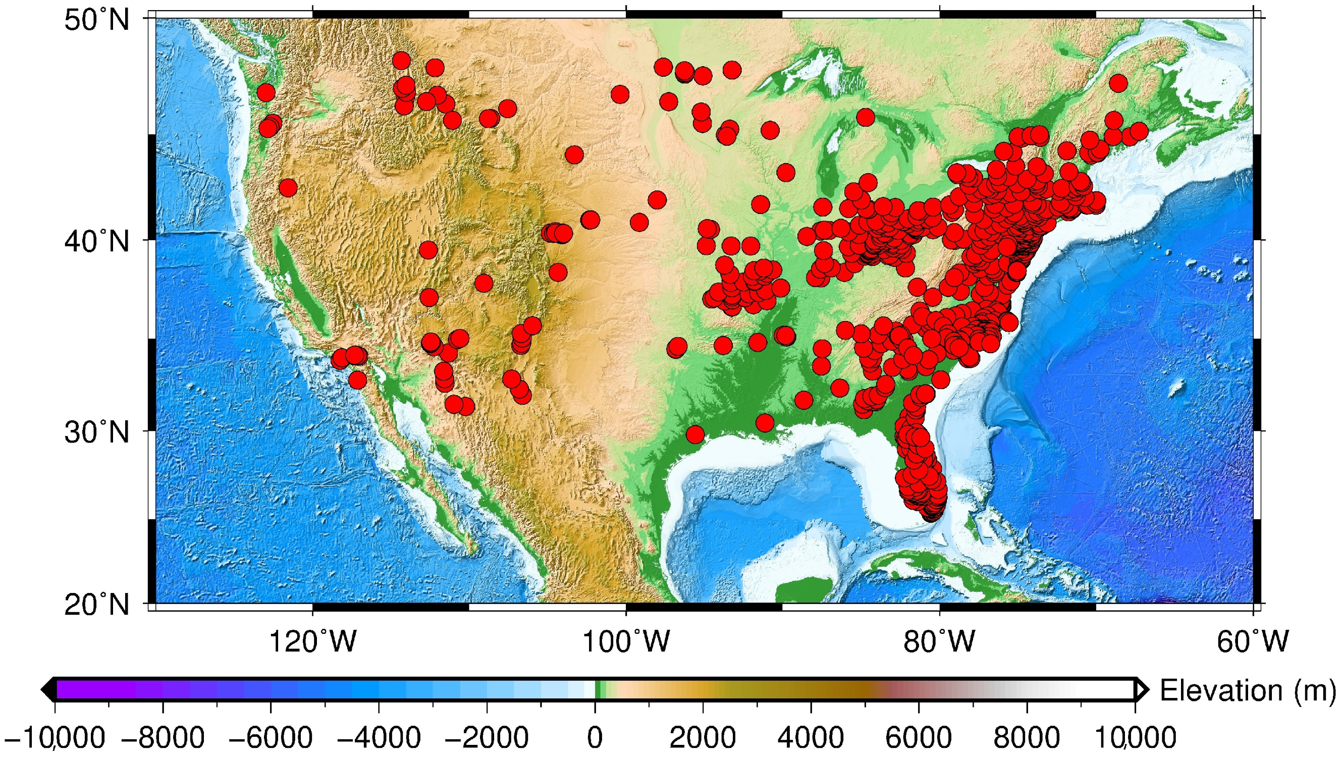
The United States Geological Survey (USGS) maintains more than 10,000 groundwater wells to monitor groundwater levels (GWLs), water quality parameters, and other relevant data for the CONUS. In this study, GWL is explicitly defined as the depth to the water table below the land surface, meaning that a lower GWL value indicates a shallower water table. The GWL data records can date back to the 1950s, and provide reliable and comprehensive data for studies aimed at understanding groundwater resources. However, some records are missing or have been discontinued due to multiple factors, bringing about the need for alternative monitoring using remote sensing techniques. In this study, in situ observations of GWL data were freely accessed through the Global Groundwater Monitoring Network (GGMN) dataset via https://ggmn.un-igrac.org/ (accessed on 10 March 2026) [43]. The entire research time span of this dataset contains GWL records spanning from 2004 to 2023 at monthly temporal resolutions, which is consistent with the remote sensing data below. The selection criteria required a monitoring period from 2004 to 2023 with a minimum data validity rate of 80%, among which over 600 wells exceeded 90% data completeness. Prior to modeling, monthly GWL values were aggregated by averaging available daily measurements, and standard quality control was applied to remove anomalies. The distribution of all wells in the CONUS is presented in Figure 1.

2.3. Remote Sensing Data

To alternatively monitor the GWL through the remote sensing technique, this study applied several satellite-based products relating to hydrological parameters, including precipitation (P), evapotranspiration (ET), and soil moisture (SM), as well as TWSA. All remote sensing data share a period from 2004 to 2023 with a temporal resolution of 1 month. A summary of these remote sensing products is presented in

Table 1. Summary of remote sensing products for hydrological parameters.

Hydrological Parameters	Remote Sensing Products	Spatial Resolution	Provider
P	GPM	0.1° × 0.1°	GES DISC
ET	MODIS	500 m × 500 m	LAADS DAAC
TWSA	GRACE	0.25° × 0.25° (~300 km)	CSR
SM	ESA CCI	0.25° × 0.25°	EODC

.

2.3.1. Precipitation (P) from GPM

As the primary input of groundwater, precipitation is a significant driver of groundwater recharge [36]. In this study, the precipitation data was obtained from NASA’s Global Precipitation Measurement (GPM) mission. The GPM IMERG product combines data from a constellation of passive microwave sensors and infrared observations, offering improved accuracy and temporal consistency compared to its predecessor, the Tropical Rainfall Measuring Mission (TRMM) [44]. The comparatively better spatial homogeneity makes it well-suited for capturing the spatiotemporal variability of precipitation across regions with diverse hydroclimatic characteristics, such as the CONUS. Specifically, the Integrated Multi-satellitE Retrievals for GPM (IMERG) L3 product version 07B was adopted, which provides quasi-global monthly precipitation estimates at a spatial resolution of 0.1° × 0.1° [45]. These data can be freely downloaded from the GES DISC at https://disc.gsfc.nasa.gov/datasets/GPM_3IMERGM_07/summary?keywords=GPM (accessed on 10 March 2026).

2.3.2. Evapotranspiration (ET) from MODIS

Evapotranspiration represents the primary avenue of water loss from the land surface to the atmosphere [38]. It is a critical component of the terrestrial water balance and impacts the variation in groundwater. ET data were acquired from the Moderate Resolution Imaging Spectroradiometer (MODIS) onboard NASA’s Terra satellites (i.e., MOD16) [46]. This product is derived using a refined Penman–Monteith equation that leverages daily meteorological reanalysis data and MODIS-derived vegetation property dynamics (e.g., land cover, leaf area index, albedo). To obtain optimal data quality, the global gap-filled version of MOD16 products (MOD16A2GF) was selected to provide ET data at a 500 m spatial resolution and an 8-day temporal resolution. It can be accessed at https://ladsweb.modaps.eosdis.nasa.gov/archive/allData/61/MOD16A2GF (accessed on 10 March 2026). Notably, the original ET data from MODIS comprises the sum of ET during these 8-day time periods (5- or 6-day for the last several days in a year). Therefore, the ET was firstly calculated at a monthly resolution based on original 8-day products as indicated by Mu et al. [47].

2.3.3. Terrestrial Water Storage Anomalies (TWSA) from GRACE

The development of satellite-based gravity measurements for hydrology has advanced the observation of terrestrial water storage (TWS). The GRACE mission and its successor (GRACE-FO), jointly developed by NASA and Deutsches Zentrumfür Luft und Raumfahrt (DLR), can capture the integrated response of TWS from space. Technically, GRACE (or GRACE-FO) measures spatiotemporal variations in the Earth’s gravity field, which are directly related to changes in terrestrial water storage. After removing a prior background model (e.g., non-tidal atmospheric and oceanic loading) and correcting for Glacial Isostatic Adjustment (GIA) and potential leakage effects along coastal areas, it provides time-varying gravity fields primarily representing TWSA on land. To maintain the optimum consistency between the GRACE and GRACE-FO measurements, the reprocessed GRACE/GRACE-FO RL06.3 Mascon Solutions provided by the CSR (RL0603) was adopted [48]. The spatial resolution of this product is 0.25° × 0.25°, which is denser than the Spherical Harmonic (SH) solutions [49]. The GRACE RL0603 product can be downloaded from the website at https://www2.csr.utexas.edu/grace/RL06_mascons.html (accessed on 10 March 2026). It is important to note that while the CSR Mascon product provides data on a nominal 0.25° × 0.25° grid, its effective spatial resolution is inherently coarser (approximately 300 km). Therefore, in the context of this well-specific monitoring system, the GRACE TWSA data is not intended to represent a physically downscaled point measurement. Instead, it serves to capture the regional-scale terrestrial water storage variation, acting as a macro-scale hydrological background forcing that, when combined with finer-scale remote sensing inputs, helps model the localized groundwater dynamics. In addition, several months of TWSA measurements were missing from the GRACE and GRACE-FO data due to equipment aging and the transition period (i.e., 2017–2018) between these two phases. This data gap was compensated based on the algorithm proposed by Gauer et al. through the Multichannel Singular Spectrum Analysis (MSSA) [50]. To strictly prevent data leakage and the introduction of future information into the model evaluation, the MSSA gap-filling was performed using only the TWSA records from the modeling period (2004 to 2019). Data from the independent testing period (2020 to 2023) were entirely excluded from this reconstruction process.

2.3.4. Soil Moisture (SM) from ESA CCI

Soil moisture is another critical linkage for land surface processes and groundwater recharge. Soil moisture represents the partitioning between water that is retained in the root zone, which further percolates downward to recharge the groundwater storage. Therefore, soil moisture is also an important hydrological parameter to be considered in monitoring GWL using the remote sensing technique. This study utilizes the European Space Agency Climate Change Initiative (ESA CCI) SM combined product v09.1 [51]. The ESA CCI combined product is not an SM dataset from one sole satellite mission, but rather integrates observations from multiple active and passive microwave sensors onboard several platforms to achieve better coverage and performance [52]. It is available at the website https://data.ceda.ac.uk/neodc/esacci/soil_moisture/ (accessed on 10 March 2026). The resolution of this product is 0.25° × 0.25° on a spatial scale and 1 day on a temporal scale in the unit of m³/m³. In contrast to evapotranspiration, the daily records within a month were averaged to obtain the monthly SM data to coincide with other hydrological parameters.

3. System Architecture and Methodology

3.1. System Architecture

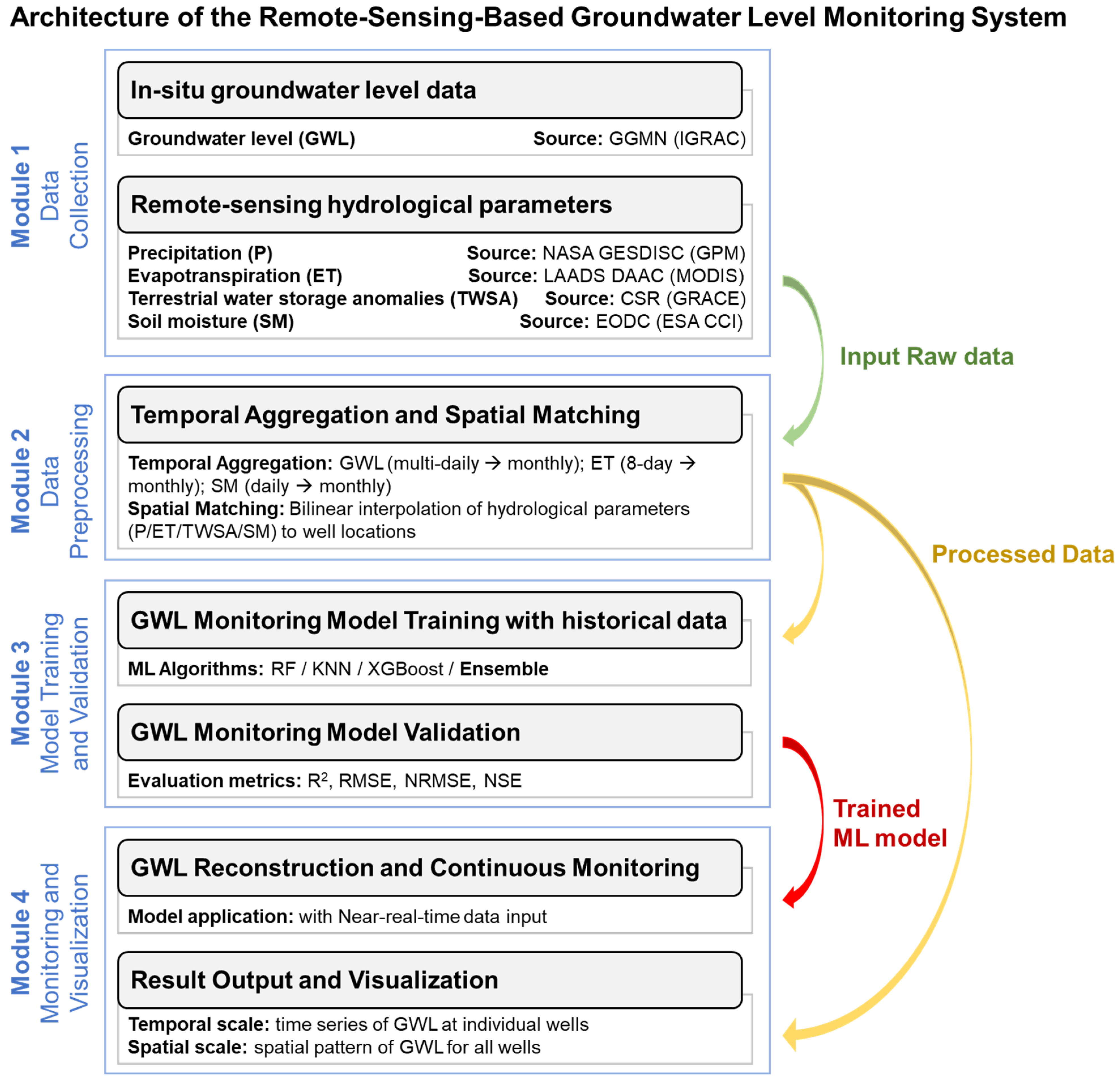
To reconstruct groundwater level time series using multi-source remotely sensed hydrological parameters, a structured monitoring system was designed. The overall architecture of the proposed remote sensing-based groundwater level monitoring system is illustrated in Figure 2. The system consists of four interconnected modules: data collection, data preprocessing, model training and validation, and monitoring and visualization. The details of each module are presented in the following subsections.

3.1.1. Module 1: Data Collection

Module 1 involves the acquisition of both in situ groundwater observations and remotely sensed hydrological parameters, which together constitute the input data of the monitoring system. These datasets can be categorized into two groups.

• In situ GWL data are obtained from monitoring wells provided by the GGMN. These observations serve as the reference data for model training and validation.
• Multi-source remote sensing hydrological parameters (i.e., P, ET, TWSA, and SM) are collected to represent the primary components of the terrestrial water balance. These parameters provide spatially continuous hydrological information that can be associated with groundwater dynamics at well locations.

The datasets obtained in this module form the raw input data for subsequent preprocessing and model development.

3.1.2. Module 2: Data Preprocessing

Module 2 performs temporal aggregation and spatial matching to ensure consistency among datasets with different temporal and spatial resolutions. This module transforms the raw input datasets into well-specific hydrological feature time series for subsequent model development.

• Temporal aggregation: To ensure temporal consistency, all datasets are unified to a monthly time scale. Different aggregation strategies are applied according to the physical characteristics of each variable. For state variables such as GWL and SM, monthly averages are calculated from daily or multi-daily records. For flux variables like ET, monthly cumulative values are derived. Variables originally provided at monthly resolution (i.e., P and TWSA) are used directly without additional temporal aggregation.
• Spatial matching: Remote-sensing hydrological parameters are spatially interpolated to individual well locations using bilinear interpolation from their original gridded format, as commonly adopted in previous studies (e.g., [53,54]). For a specific well located at coordinates $\left(x,y\right)$, surrounded by four adjacent grid centers $Q_{11}(x_1,y_1)$, $Q_{12}(x_1,y_2)$, $Q_{21}(x_2,y_1)$, and $Q_{22}(x_2,y_2)$. In this case, the interpolated parameter value $V\left(x,y\right)$ is calculated through linear interpolations in both the $x$ and $y$ directions as follows

$$V\left(x,y_1\right)={\displaystyle \frac{x_2-x}{x_2-x_1}}V\left(Q_{11}\right)+{\displaystyle \frac{x-x_1}{x_2-x_1}}V\left(Q_{21}\right)$$

(1)

$$V\left(x,y_2\right)={\displaystyle \frac{x_2-x}{x_2-x_1}}V\left(Q_{12}\right)+{\displaystyle \frac{x-x_1}{x_2-x_1}}V\left(Q_{22}\right)$$

(2)

$$V\left(x,y\right)={\displaystyle \frac{y_2-y}{y_2-y_1}}V\left(x,y_1\right)+{\displaystyle \frac{y-y_1}{y_2-y_1}}V\left(x,y_2\right)$$

(3)

This mathematical process ensures the extraction of continuous, well-specific time series for P, ET, TWSA, and SM that align precisely with the geographic location of each monitoring well.

A consistent and spatially aligned dataset is constructed through temporal aggregation and spatial matching, forming the processed input features for the machine learning models.

3.1.3. Module 3: Model Training and Validation

Module 3 involves the construction of the GWL monitoring model based on the processed hydrological parameters generated in Module 2. This module integrates machine learning algorithms to characterize the relationship between remotely sensed hydrological parameters and in situ GWL observations.

The module consists of two main components: model training and model validation. It is important to explicitly clarify the model training strategy adopted in this system: the machine learning models were trained independently for each individual well, rather than jointly for all wells or by regional groups. Consequently, for each algorithm (KNN, RF, XGBoost), approximately 770 separate and independent models were constructed. During the training stage, these ML algorithms were employed to establish the specific nonlinear relationships between the input variables (P, ET, TWSA, SM, and time parameter) and the target GWL exclusively using the historical time series of that specific well. This well-specific training strategy is highly advantageous, as it ensures that each model inherently learns and adapts to the unique, localized hydrogeological properties specific to its corresponding monitoring well.

In the validation stage, the trained models are evaluated using independent datasets to assess their modeling performance. Evaluation metrics are applied to quantify the agreement between simulated and observed GWL values. The output of this module is a set of trained machine learning models that can be applied for GWL reconstruction and continuous monitoring.

3.1.4. Module 4: Monitoring and Visualization

Module 4 represents the operational component of the proposed monitoring system. In this stage, the trained ML models generated in Module 3 are applied to remotely sensed hydrological parameters to reconstruct GWL at individual well locations.

With the continuous input of monthly remote sensing data, the trained models generate reconstructed GWL time series for each monitoring well. This process enables sustained groundwater monitoring even when in situ observations are incomplete or temporarily unavailable. The monitoring outputs are presented at both temporal and spatial scales, enabling time-series analysis at individual wells and visualization of regional groundwater dynamics.

3.2. Experimental Design for System Validation

To evaluate the effectiveness of the proposed remote sensing-based GWL monitoring system, a validation experiment was designed based on real data from 20 years (2004 to 2023) across the CONUS. The historical in situ observations of GWL were used to train ML-based models, and the model performance was assessed using an independent test dataset.

First, all data including remotely sensed hydrological parameters (P, ET, TWSA, and SM) and in situ GWL records were extracted and matched on both spatial and temporal scales to construct the dataset. Each sample of the dataset consists of four input variables (i.e., hydrological parameters) and the target variable GWL at a specific monitoring well and time epoch. Since GWL observations occasionally contain missing records, samples with unavailable GWL values were excluded from model training and evaluation.

The dataset was then divided chronologically, and four subsets were defined to support hyperparameter optimization, model construction and model validation. The detailed time periods for the four subsets are:

• Hyperparameter training: 2004–2016;
• Hyperparameter validation: 2017–2019;
• Model training: 2004–2019;
• Model testing: 2020–2023.

Data from 2004 to 2016 were used as the training subset for model hyperparameter optimization. Data from 2017 to 2019 served as a validation subset for evaluating candidate hyperparameter configurations. The hyperparameters of the machine learning models were automatically optimized using the Optuna framework [55]. Unlike traditional grid or random search, Optuna implements an advanced Bayesian optimization strategy, specifically utilizing the Tree-structured Parzen Estimator (TPE) algorithm. This approach probabilistically models the relationship between hyperparameters and model performance, dynamically focusing the search on the most promising hyperparameter regions while efficiently pruning unpromising trials. This automated and highly efficient tuning process is particularly essential for our proposed system, as it requires optimizing approximately 770 independent, well-specific models for each machine learning algorithm. The specific hyperparameter search ranges defined for each ML algorithm (RF, KNN, XGBoost) are detailed in

Table A1. Hyperparameter search ranges for the machine learning models optimized via Optuna.

Algorithms	Hyperparameters	Search Ranges
RF	n_estimators	[100, 150, 200, 250]
	max_depth	[1, 2, 3, 4, 5, 6, 7, 8, 9, 10]
	min_samples_split	2, 15
	min_samples_leaf	1, 19, step = 1
	random_state	42
	verbose	0
KNN	n_neighbors	[1, 2, 3, 4, 5, 6]
	leaf_size	[1, 5, 10, 15, 20, 25, 30]
	p	[1, 2]
	weights	distance
XGBoost	n_estimators	[50, 100, 150, 200, 250, 300, 350, 400, 450, 500]
	max_depth	[1, 2, 3, 4, 5, 6]
	learning_rate	0.01, 0.05, step = 0.005
	random_state	42

in Appendix A.

After the optimal hyperparameters had been obtained, the models were retrained using the complete training dataset from 2004 to 2019 to fully exploit the available historical observations. Finally, an independent testing period from 2020 to 2023 was used to evaluate model performance. During this stage, the trained models were applied to reconstruct GWL using only remotely sensed hydrological parameters, and the reconstructed results were compared with in situ observations to assess the monitoring capability of the proposed system.

3.3. Machine Learning Algorithms

To reconstruct GWL from remotely sensed hydrological parameters, three widely used machine learning algorithms were employed in this study, including Random Forest (RF), K-Nearest Neighbor (KNN), and Extreme Gradient Boosting (XGBoost). These algorithms represent different modeling paradigms and have demonstrated strong capability in capturing nonlinear relationships in hydrological systems. They have therefore been widely applied in hydrological and water resources studies (e.g., [56,57,58]). Additionally, an ensemble model was constructed by averaging the reconstructed GWL values from RF, KNN, and XGBoost. By comparing their performance, the robustness and reliability of the proposed monitoring system can be evaluated.

3.3.1. Random Forest (RF)

RF is an ensemble learning algorithm based on multiple decision trees [59]. It constructs a collection of decision trees using bootstrap sampling of the training data, while a random subset of input variables is selected at each node for tree splitting. This strategy introduces randomness into the model construction process, which effectively reduces overfitting and improves model robustness.

To reconstruct the GWL, the RF output is obtained by averaging the outputs of all decision trees in the forest:

$${\widehat{y}}_{RF}={\displaystyle \frac{1}{N}}{\displaystyle \sum _{i=1}^N}{f}_i(P,ET,TWSA,SM,Y,M_{sin},M_{cos})$$

(4)

where ${\widehat{y}}_{RF}$ denotes GWL output using RF, N represents the number of decision trees, $f_i$ denotes the prediction of the i-th tree, and P, ET, TWSA, SM, Y (Year), $M_{sin}$, and $M_{cos}$ represent the input feature vectors. The cyclical month features $M_{sin}$ and $M_{cos}$ are defined as

$$M_{sin}=\sin \left(2\pi \cdot {\displaystyle \frac{M}{12}}\right)$$

(5)

$$M_{cos}=\cos \left(2\pi \cdot {\displaystyle \frac{M}{12}}\right)$$

(6)

where M represents the month from 1 to 12. It should be noted that the inclusion of the temporal feature Y (Year) serves a specific modeling purpose. Since direct, high-resolution data on progressive anthropogenic activities (e.g., continuous groundwater pumping and land-use changes) are difficult to obtain. In this case, time parameters (including Y) can act as an alternative to capture localized, long-term unobserved anthropogenic trends. Although introducing a temporal feature carries a potential risk of overfitting a time trend instead of learning hydrological mechanisms, this risk is mitigated by the inherent mechanism of tree-based models (such as RF and XGBoost). Since tree-based models cannot extrapolate numerical values beyond the maximum range seen during training, the influence of the Y feature saturates during the independent testing period (2020 to 2023). Consequently, the accurate predictions achieved in the testing phase demonstrate that the models successfully capture the physically meaningful hydrological responses driven by P, ET, TWSA, and SM, rather than merely continuing a statistical timeline.

3.3.2. K-Nearest Neighbor (KNN)

KNN is a non-parametric machine learning algorithm that predicts the target variable based on the similarity between samples in the feature space [60]. Instead of constructing an explicit model during training, KNN stores the training data and performs predictions by identifying the k-nearest samples to a query point according to a distance metric. In this study, the Euclidean distance was used to measure the similarity between feature vectors. The Euclidean distance between two feature vectors (${\mathrm{x}}_{\mathrm{i}},{\mathrm{x}}_{\mathrm{j}}$) is defined as

$$d(x_i,x_j)=\sqrt{{\displaystyle \sum _{m=1}^p}{(x_{i,m}-x_{j,m})}^2}$$

(7)

where p denotes the number of input features and $x_{i,m}$ represents the m-th feature of the sample. Prior to distance calculation, all input features were standardized to eliminate the influence of different variable scales.

After identifying the k nearest neighbors based on the distance d, the reconstructed GWL is obtained by averaging the GWL values of these neighboring samples:

$${\widehat{y}}_{KNN}={\displaystyle \frac{1}{k}}{\displaystyle \sum _{i=1}^k}{\widehat{y}}_i$$

(8)

where ${\widehat{y}}_{KNN}$ denotes the reconstructed GWL using the KNN model, k represents the number of nearest neighbors, and ${\widehat{y}}_i$ denotes the observed GWL of the i-th nearest neighbor in the training dataset.

3.3.3. Extreme Gradient Boosting (XGBoost)

XGBoost is an efficient implementation of gradient boosting decision trees designed for scalable machine learning tasks [61]. It constructs an ensemble of decision trees sequentially, where each new tree is trained to minimize the residual errors of the previous model. By iteratively improving the model, XGBoost is able to capture complex nonlinear relationships between input variables and the target variable.

The objective function of XGBoost consists of a loss function and a regularization term, which can be expressed as

$$L={\displaystyle \sum _{i=1}^p}l(y_i,{\widehat{y}}_i)+{\displaystyle \sum _{j=1}^q}\mathsf{\Omega }(f_j)$$

(9)

where l denotes the loss function measuring the difference between the observed ($y_i$) and estimated GWL (${\widehat{y}}_i$), q represents the number of decision trees, and $\mathsf{\Omega }\left(f_j\right)$ is the regularization term that controls model complexity to prevent overfitting.

3.3.4. Ensemble Model

To further improve the robustness of the GWL monitoring system, an ensemble model was constructed by combining the outputs of three ML models (i.e., RF, KNN, and XGBoost). This strategy can reduce the influence of individual model biases and improve overall performance. In this study, the ensemble output was obtained using a weight-mean ensemble strategy:

$$w_i={\displaystyle \frac{\frac{1}{{\epsilon }_i}}{\frac{1}{{\epsilon }_{RF}}+\frac{1}{{\epsilon }_{KNN}}+\frac{1}{{\epsilon }_{XGB}}}}$$

(10)

$${\widehat{y}}_{ENS}=w_{RF}\times {\widehat{y}}_{RF}+w_{KNN}\times {\widehat{y}}_{KNN}+w_{XGB}\times {\widehat{y}}_{XGB}$$

(11)

where $w_i$ is the weight for each method. ${\widehat{y}}_{ENS}$ denotes the reconstructed GWL from the ensemble model, and ${\widehat{y}}_{RF}$, ${\widehat{y}}_{KNN}$, and ${\widehat{y}}_{XGB}$ represent the reconstructed GWL obtained from the RF, KNN, and XGBoost models, respectively. ${\epsilon }_{RF}$, ${\epsilon }_{KNN}$, and ${\epsilon }_{XGB}$ are the errors (indicated by RMSE) between the reconstructed and observed GWL for the training period. ${\epsilon }_i$ is the error for a specific method. By combining multiple models with different learning mechanisms, the ensemble approach can improve the stability and reliability of GWL reconstruction.

3.4. Evaluation Metrics

To quantitatively evaluate the performance of the proposed GWL monitoring system, four commonly utilized statistical metrics were adopted, including the coefficient of determination (R²), root mean square error (RMSE), normalized root mean square error (NRMSE), and Nash–Sutcliffe efficiency (NSE). These metrics are widely used in hydrological modeling studies [37,62] to assess the agreement between reconstructed and observed GWL.

The coefficient of determination R² quantifies the strength of the linear relationship between observed and reconstructed GWL and is calculated as the square of the Pearson correlation coefficient as follows:

$$R^2={\displaystyle \frac{{\left[{\sum }_{i=1}^n\left(y_i-\overline{y}\right)\left({\widehat{y}}_i-\overline{\widehat{y}}\right)\right]}^2}{{\sum }_{i=1}^n{(y_i-\overline{y})}^2{\sum }_{i=1}^n{({\widehat{y}}_i-\overline{\widehat{y}})}^2}}$$

(12)

where $\overline{y}$ and $\overline{\widehat{y}}$ are the average of $y_i$ and ${\widehat{y}}_i$, respectively; n is the number of samples.

The RMSE quantifies the average magnitude of reconstruction errors, which can be expressed as:

$$RMSE=\sqrt{{\displaystyle \frac{1}{n}}{\displaystyle \sum _{i=1}^n}{({\widehat{y}}_i-y_i)}^2}$$

(13)

The NRMSE accounts for the differences in the observed GWL ranges; it is calculated by dividing the RMSE by the range of observed GWL values:

$$NRMSE={\displaystyle \frac{RMSE}{\max \left(y\right)-\mathrm{m}\mathrm{i}\mathrm{n}\left(y\right)}}={\displaystyle \frac{\sqrt{\frac{1}{n}{\displaystyle {\sum }_{i=1}^n}{\left({\widehat{y}}_i-y_i\right)}^2}}{\max \left(y\right)-\min \left(y\right)}}$$

(14)

The NSE is an efficiency coefficient for hydrological models [63] and evaluates the performance of the model output relative to the mean of the observations:

$$NSE=1-{\displaystyle \frac{{\sum }_{i=1}^n{({\widehat{y}}_i-y_i)}^2}{{\sum }_{i=1}^n{(y_i-\overline{y})}^2}}$$

(15)

The NSE ranges from −∞ to 1, with higher values indicating better model performance. In general, higher values of R² and NSE and lower values of RMSE and NRMSE indicate better model performance.

4. Results

This section presents the results of the proposed GWL monitoring system and the corresponding discussions. First, cross-correlation analysis is conducted to investigate the relationships and time lags between GWL and four hydrological parameters. Then, the performance of different machine learning models for GWL reconstruction and monitoring is evaluated. Finally, the spatiotemporal characteristics of the monitoring results are analyzed across all monitoring wells.

4.1. Cross-Correlation Analysis Between Hydrological Parameters and GWL

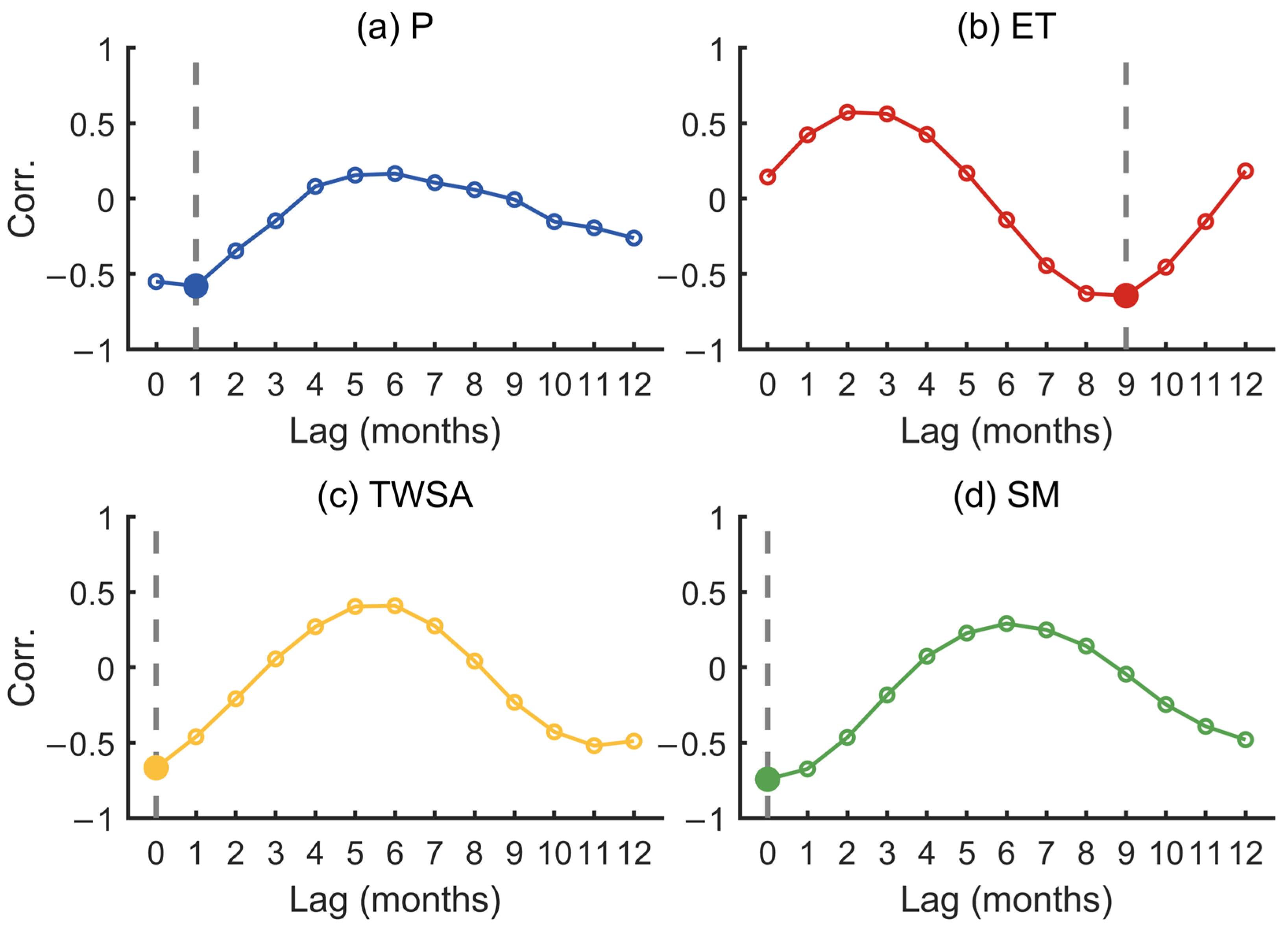
To investigate the temporal relationships between GWL and four remotely sensed hydrological parameters, cross-correlation analysis was conducted. To strictly avoid any data leakage from the future, this analysis was performed exclusively using data from the model training period (2004 to 2019) to determine the highest correlations and the corresponding optimal time lags [64]. Once determined, these optimal lags were fixed and applied unchanged to shift the input features during the independent testing period (2020 to 2023). Note that lag values ranging from 0 to 12 months were considered, where the remote sensing time series were shifted forward relative to GWL to identify the delayed groundwater response to hydrological forcing. Prior to calculating the cross-correlations, the long-term linear trends were removed from all time series to eliminate spurious correlations caused by multi-year long-term drifts. Furthermore, considering that the relationships between GWL and the four hydrological parameters may not be perfectly linearly correlated, the cross-correlation was calculated using the Spearman rank correlation coefficient. To visually illustrate the cross-correlation calculation procedure, a representative monitoring well was first selected (Figure 3). This specific well was chosen because it possesses a highly complete and continuous observational record without missing data, and its temporal dynamics closely represent the median statistical behavior of the entire dataset, making it an ideal typical example.

It can be observed that all four parameters exhibit negative correlations with GWL. This behavior is perfectly consistent with the definition of GWL in this manuscript, where GWL represents the depth to the water table below the land surface. Physically, an increase in groundwater storage, for example due to higher precipitation, soil moisture, or terrestrial water storage, elevates the water table. thereby decreasing the GWL (depth) value. Precipitation reaches its strongest correlation (−0.58) at a lag of 1 month, indicating that groundwater responds relatively rapidly to rainfall recharge. In contrast, evapotranspiration shows the longest delay, with the strongest correlation (−0.64) occurring at a lag of 9 months, suggesting that the influence of ET on groundwater mainly reflects longer-term water balance processes. For TWSA and SM, the strongest correlations are observed at lag 0, with correlation coefficients of approximately −0.67 and −0.74, respectively, revealing relatively synchronous variations between groundwater level and these hydrological storage indicators at this location.

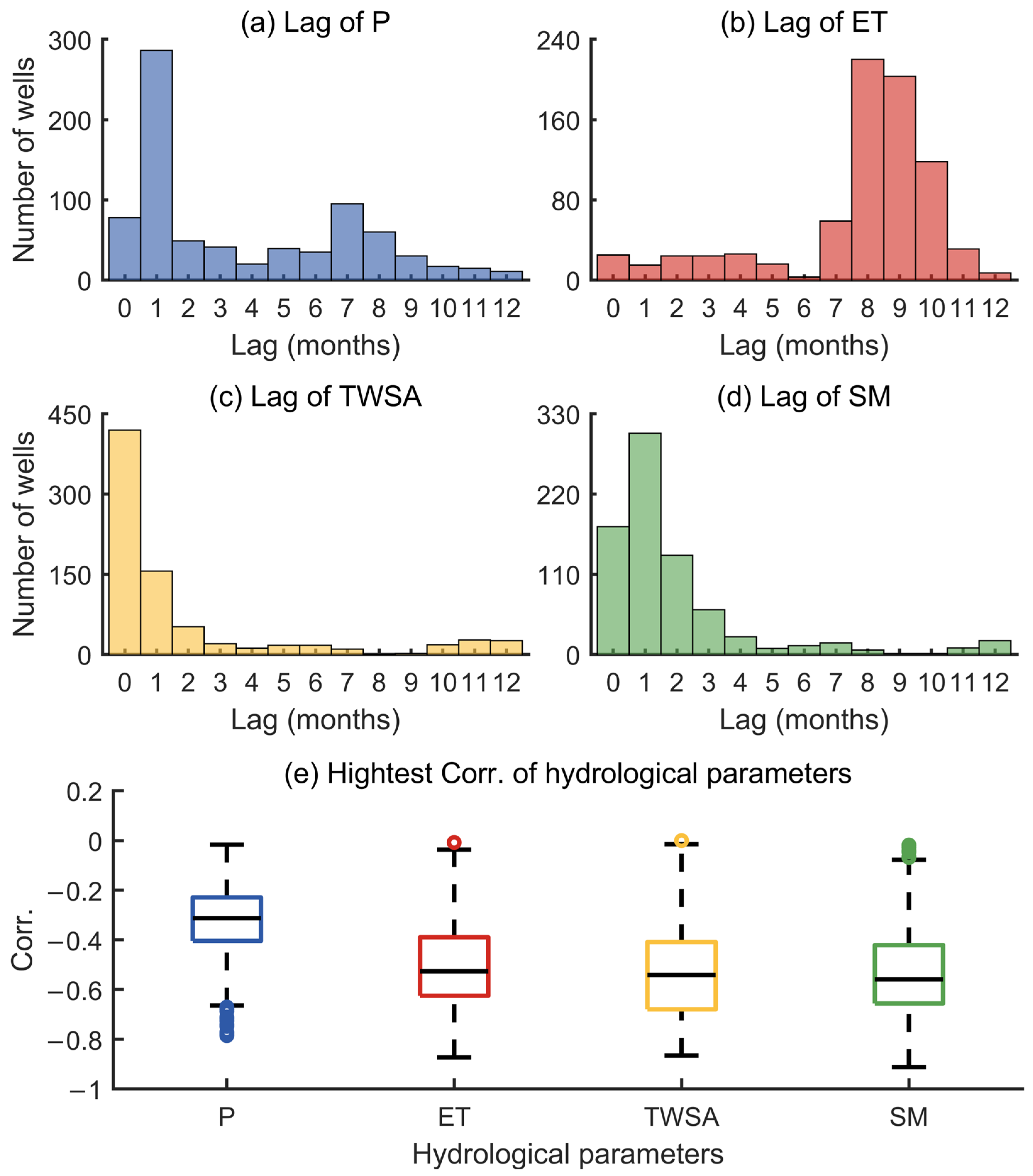
Following this individual demonstration, the same procedure was systematically applied to all ~770 monitoring wells individually and then summarized for all wells to derive regional summary statistics. To further examine the correlation characteristics for all monitoring wells, the histograms of the distributions of optimal time lags for each hydrological variable are summarized in Figure 4a–d. The results show that the optimal lag for precipitation is concentrated between 0 and 1 month, with most wells showing a lag of 1 month. This suggests that rainfall typically influences groundwater levels within a short time period. Similarly, soil moisture also had lag values distributed between 0 and 2 months, and a dominant lag of 1 month. For the TWSA, the strongest responses occurred at lag 0, indicating that groundwater variations are closely associated with large-scale terrestrial water storage changes. In contrast, evapotranspiration exhibits longer lag periods, mainly distributed between 8 and 10 months, with peaks at 8 and 9 months. This delayed response is most likely due to the cumulative influence of evapotranspiration on groundwater through the long-term depletion of subsurface water storage.

For the maximum correlation, the correlating relationships for all hydrological parameters are summarized as a boxplot in Figure 4e. The median correlations are −0.31, −0.53, −0.54, and −0.56 for P, ET, TWSA, and SM, respectively. Compared with precipitation, ET, TWSA, and SM all exhibit stronger correlations with GWL variations. This result suggests that groundwater dynamics are more strongly linked to integrated hydrological storage and long-term water balance processes than to precipitation inputs. After determining the optimal time lags, the time series of four remotely sensed hydrological parameters were shifted accordingly for each well. The shifted time series can be used as model inputs to improve the performance of the subsequent GWL reconstruction step.

While the cross-correlation analysis successfully identifies the optimal time lags to maximize the predictive performance of the machine learning algorithms, it is crucial to emphasize that “correlation does not necessarily imply causation.” The statistically derived lag times shown in Figure 4 represent “apparent lags” that lump together natural hydrogeological processes, deep aquifer dynamics, and unquantified human interventions, rather than purely vertical physical travel times.

First, the widespread human-induced groundwater fluctuations in heavily managed areas significantly alter natural correlations. For instance, an observed strong correlation between GWL decline and high Evapotranspiration (ET) does not imply that ET directly evaporates deep groundwater. Instead, ET acts as a climatic proxy for human behavior. Specifically, high ET and low Precipitation (P) trigger intensive agricultural pumping, which causes immediate GWL drawdown. Consequently, the statistical models exploit these meteorological variables to implicitly capture human-induced extraction patterns.

Second, the physical interpretation of longer lag times (e.g., 8~12 months) requires caution. An extended lag does not strictly dictate that a single rainfall event requires 12 months to vertically percolate to the water table. In unconfined aquifers with thick vadose zones, deep percolation can indeed take months to years. However, in other contexts, these long lags often reflect the horizontal propagation of pressure pulses along extensive regional flow paths, or the inter-annual “memory effect” of the aquifer, where current GWL variations are driven by the accumulated water balance of previous multi-season climatic cycles.

Finally, the degree of physical coupling depends heavily on the aquifer type. For unconfined aquifers, local precipitation and soil moisture exhibit direct, causal relationships with aquifer recharge. Conversely, for confined aquifers, the water table is separated by impermeable layers and is largely decoupled from local surface infiltration. In such cases, the correlations identified with local P or SM may be spurious, or they may simply reflect broader regional climate synchrony rather than localized vertical recharge. Therefore, the optimal lags utilized in this study function primarily as optimized, data-driven parameters for feature engineering, designed to capture complex, site-specific hydro-climatic signatures rather than universal physical constants.

4.2. Evaluation of System Monitoring Performance

To evaluate the feasibility of the proposed GWL monitoring system, the performance of the reconstructed GWL using remotely sensed hydrological variables with four machine learning algorithms was tested during the independent period from 2020 to 2023. The performance was quantitatively assessed using four statistical metrics: R², RMSE, NRMSE, and NSE.

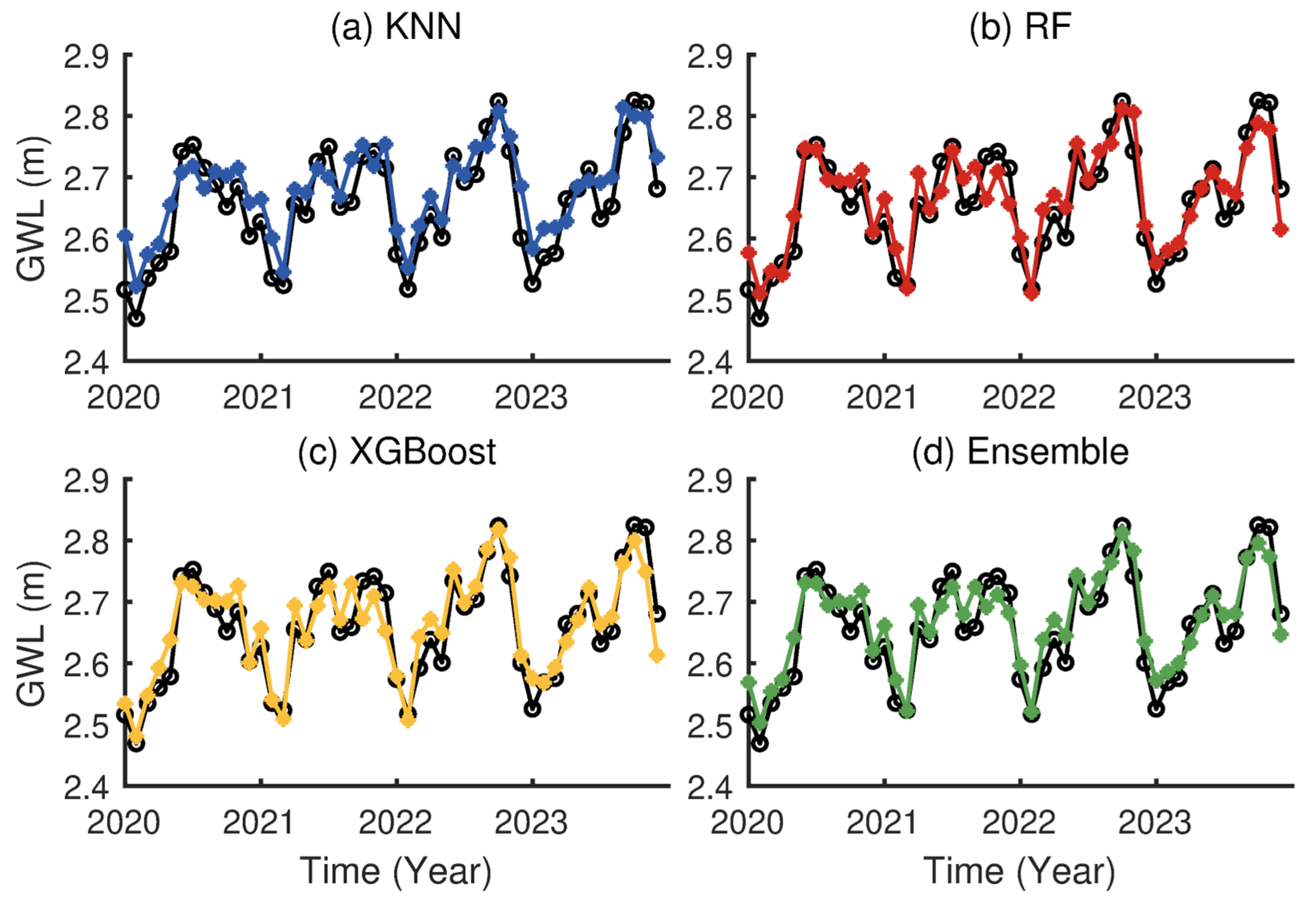
To illustrate the performance of GWL monitored through the system, the time series of the observed and reconstructed GWL at the median-performance well (at 31.5924°N, 84.3421°E) during the independent period from 2020 to 2023 was selected and presented, as shown in Figure 5. The four subplots of Figure 5 contain the in situ measured and reconstructed GWL using different algorithms. Note that the y-axis in Figure 5 represents the depth to the water table below the land surface. A good performance for GWL in all four algorithms can be observed at this well. Among different algorithms, the results show that the Ensemble model provides the best performance, with the highest R² (0.898), lowest RMSE (0.032 m), lowest NRMSE (9.03%), and highest NSE (0.868). This indicates that the Ensemble model most accurately tracks the observed groundwater dynamics. In contrast, the KNN model exhibits the weakest performance, with an R² of 0.864, RMSE of 0.041 m, NRMSE of 11.77%, and the lowest NSE of 0.776. This suggests that KNN struggles to capture the variability in GWL using remotely sensed hydrological variables. The RF and XGBoost models perform generally well, but they both show slightly higher RMSE and NRMSE values compared to the Ensemble model.

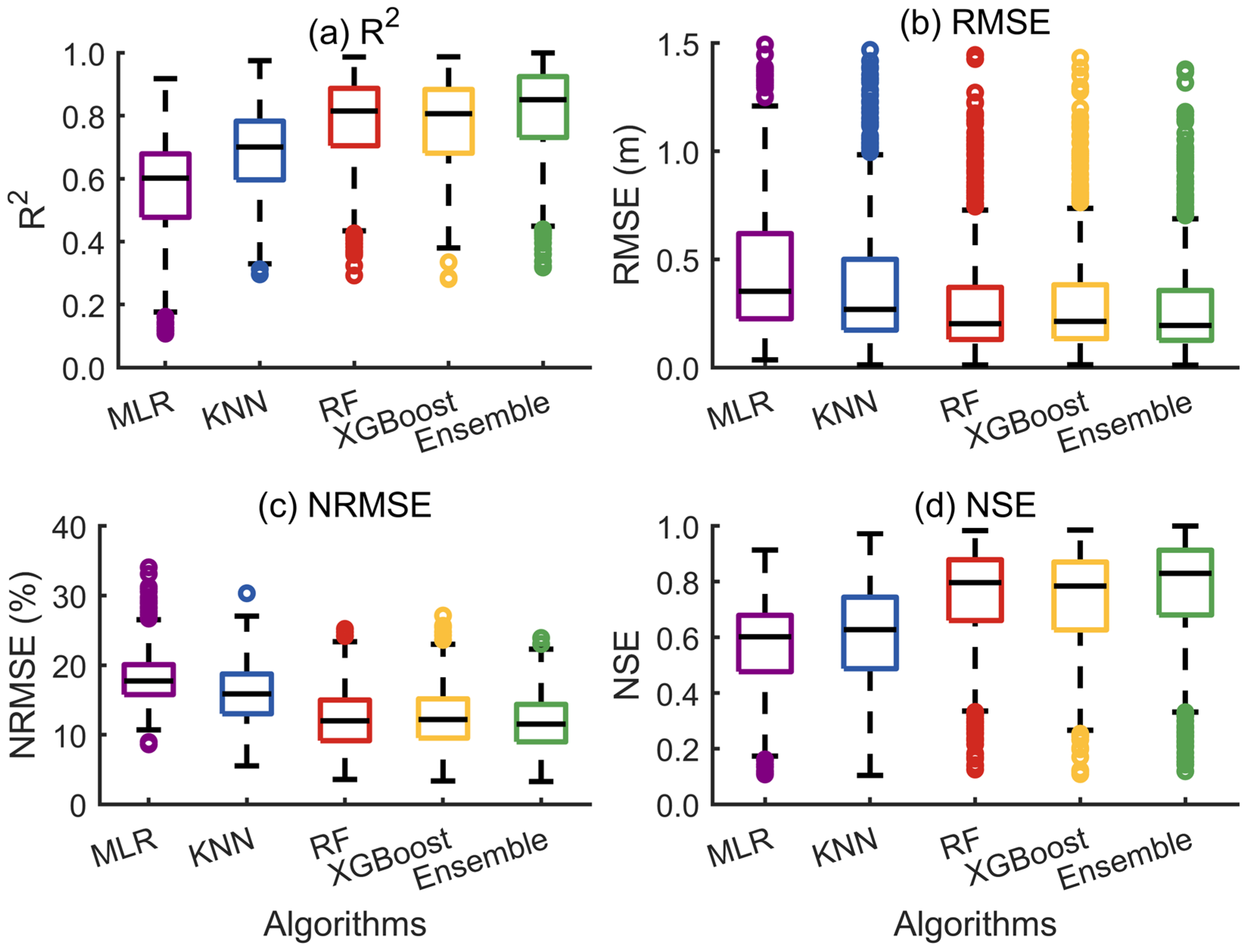
Afterwards, the performance of the four ML models across all wells was evaluated. To rigorously evaluate the superiority of the ML algorithms, a traditional model based on Multiple Linear Regression (MLR) was introduced as a baseline comparison in this study. The MLR model was trained using the consistent feature and dataset as the ML algorithms, where the inclusion of temporal variables effectively served as a harmonic regression to capture linear trends and seasonal climatology. The comparative statistical results across all wells for the individual ML models, the Ensemble model, and the baseline of MLR are summarized in

Table 2. Summarization of evaluation metrics (including mean, median, STD, and IQR) for GWL monitored with different algorithms during the test period.

Models	Evaluation Metrics
	R2		RMSE (m)		NRMSE (%)		NSE
	Mean & STD	Median & IQR	Mean & STD	Median & IQR	Mean & STD	Median & IQR	Mean & STD	Median & IQR
MLR	0.57 ± 0.15	0.60 ± 0.20	0.65 ± 1.16	0.35 ± 0.39	14.0 ± 2.84	13.6 ± 3.31	0.57 ± 0.16	0.60 ± 0.20
KNN	0.69 ± 0.13	0.70 ± 0.19	0.47 ± 0.75	0.27 ± 0.33	15.9 ± 4.10	15.9 ± 5.71	0.60 ± 0.19	0.63 ± 0.26
RF	0.78 ± 0.14	0.82 ± 0.18	0.35 ± 0.53	0.20 ± 0.24	12.2 ± 4.19	12.0 ± 5.84	0.74 ± 0.18	0.80 ± 0.22
XGBoost	0.77 ± 0.14	0.81 ± 0.20	0.36 ± 0.55	0.21 ± 0.25	12.5 ± 4.23	12.2 ± 5.63	0.73 ± 0.18	0.78 ± 0.24
Ensemble	0.81 ± 0.15	0.85 ± 0.19	0.34 ± 0.53	0.19 ± 0.23	11.8 ± 3.88	11.5 ± 5.39	0.78 ± 0.19	0.83 ± 0.23

. Note that the mean, median, standard deviation (STD), and interquartile range (IQR) of four evaluation metrics for all algorithms were presented in Table 2. In addition, Figure 6 gives the boxplots of four evaluation metrics for all in situ wells through different ML algorithms and the MLR baseline for a clearer illustration.

As presented in Figure 6 and Table 2, the proposed ML models significantly outperform the simple MLR baseline. The MLR model achieved moderate overall performance, yielding a median R² of 0.60, a median NSE of 0.60, a median RMSE of 0.35, and a median NRMSE of 13.6%. While the linear baseline successfully captures the general seasonal variability due to the harmonic temporal features, it inherently assumes that hydrological responses are purely linear and additive.

In contrast, the substantial performance gain achieved by the ML algorithms for they were able to capture the more complicated relationships between GWL and hydrological parameters, which the simple MLR fundamentally fails to resolve. Among three separate algorithms, the KNN model shows the weakest performance, with the lowest mean R² (0.69) and NSE (0.60), and the highest RMSE (0.47 m) and NRMSE (15.9%). The RF and XGBoost models perform similarly to and slightly better than the KNN. The best performance was obtained through the Ensemble model. Results exhibit that it attains the highest mean R² (0.81) and NSE (0.78), and the lowest mean RMSE (0.34 m) and NRMSE (11.8%). The best performance from the weight-mean Ensemble model explicitly demonstrates the critical advantage of ML algorithms. It is capable of capturing complex, non-linear hydrogeological interactions and threshold effects, such as the non-linear transformation of precipitation and soil moisture into groundwater recharge.

In addition, it can be observed from Figure 6 that the Ensemble model also has the smallest variability in performance across wells. This higher consistency with the observed GWL indicates that weighting combinations through results from the KNN, RF, and XGBoost algorithms can further mitigate gross error brought about by any individual ML method. In general, the results demonstrate that the proposed GWL monitoring system can effectively reconstruct groundwater level dynamics for most wells using the remotely sensed observations and ML algorithms. The ensemble strategy further improves model robustness by integrating the strengths of multiple ML algorithms. This system can serve as an alternative for monitoring groundwater variations when one specific monitoring well is no longer available.

5. Discussions

The results presented in the previous sections demonstrate the potential of the proposed monitoring system, which integrates remote sensing observations with ML for large-scale GWL reconstruction. The weight-mean ensemble model successfully captured the temporal dynamics of GWL across diverse hydrological characteristics. However, a comprehensive and objective evaluation of such a continental-scale system requires a deeper examination beyond the overall accuracy. In this subsection, we discuss the relative contribution of each feature and physical context necessary for correctly interpreting the statistical metrics across vastly different aquifers. Afterwards, the primary uncertainties and limitations inherent in the proposed system were acknowledged.

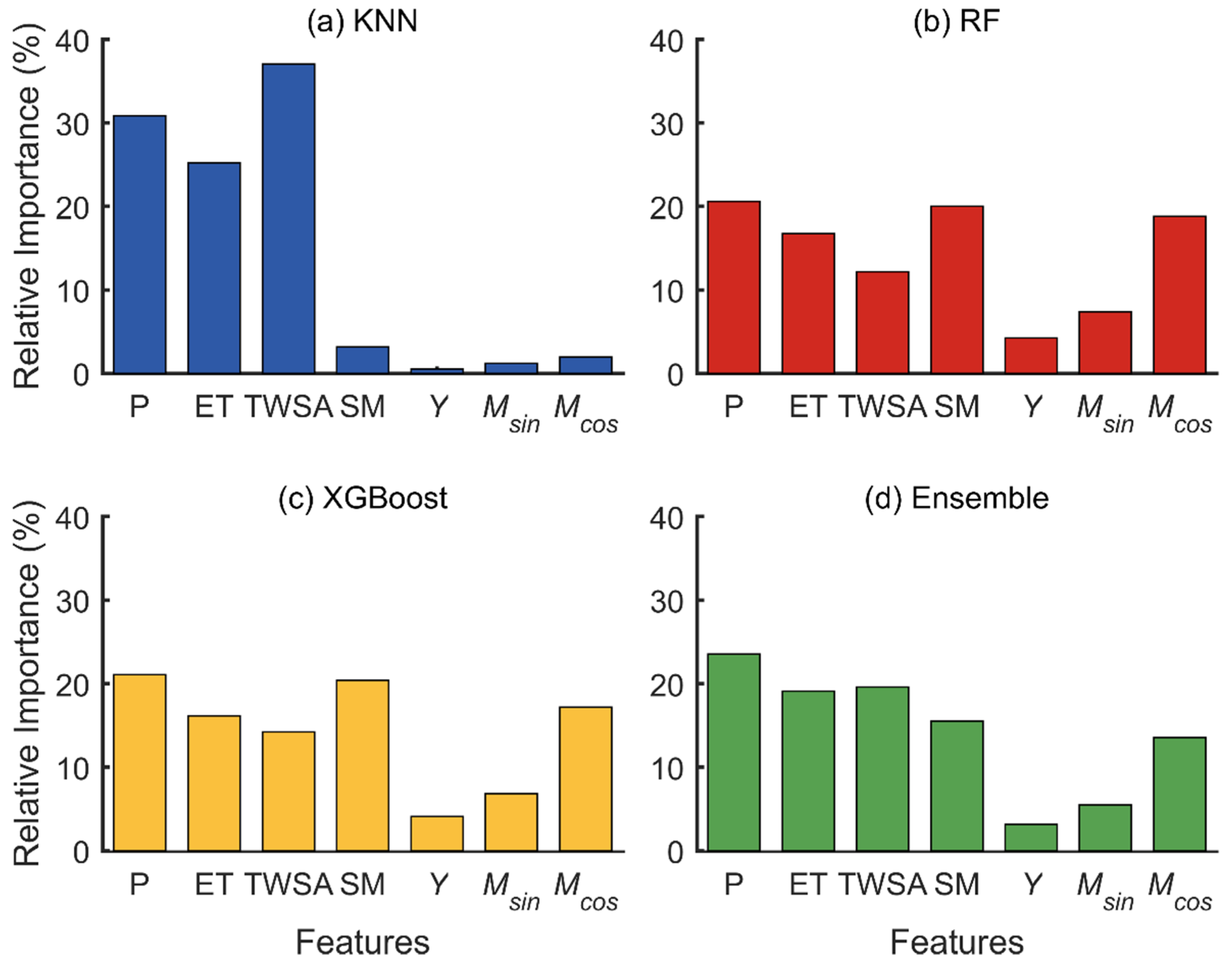
To objectively quantify the relative contributions of the hydrological and time parameters to GWL reconstruction, a feature-importance analysis using the SHapley Additive exPlanations (SHAP) framework was conducted. It should be noted that to eliminate the scale-dependency caused by the highly variable natural GWL fluctuation amplitudes across the ~770 monitoring wells, we calculated the Normalized SHAP-based Relative Contribution (RC) by normalizing the absolute SHAP impacts within each well before deriving the global regional average. The relative contributions (RC) of each feature for different algorithms are illustrated in Figure 7. As depicted in Figure 7a–c, three base models (KNN, RF, and XGBoost) exhibited distinct preferences governed by their underlying mathematical structures. The distance-based KNN model was heavily dominated by macro-scale variables such as TWSA (37.0%) and precipitation (30.8%), while tree-based models (RF and XGBoost) demonstrated a robust capacity to capture seasonal temporal patterns $M_{cos}$ (17–18%). By integrating these complementary algorithmic behaviors, the Ensemble model (Figure 7d) yielded a comprehensive and physically interpretable hierarchy of hydrological drivers. Precipitation emerged as the dominant controlling factor (23.5%), serving as the primary recharge source. This was closely followed by TWSA (19.6%) and Evapotranspiration (19.1%), representing the regional background water storage and the main discharge component, respectively. Soil Moisture (15.5%) acted as a critical intermediate buffer regulating the infiltration process. Furthermore, the limited contribution of the inter-annual Y (Year) feature (3.1%) compared to the harmonic seasonal terms (~19%) confirms that the GWL dynamics in the study area are primarily driven by intra-annual seasonal hydro-climatic cycles.

Furthermore, it is worth discussing the capacity of the selected conventional machine learning algorithms to capture temporal dependencies. While conventional models (like RF, XGBoost, and KNN) lack the internal recurrent memory states inherent in sequence-based deep learning models (such as LSTM or TCN), our framework effectively resolved this limitation through rigorous physical feature engineering. First, the cross-correlation lag analysis explicitly embedded the historical “memory” and delayed response of the aquifers into the input feature space. Second, the inclusion of explicitly engineered temporal parameters, the harmonic seasonal terms ($M_{sin}$, $M_{cos}$) and the inter-annual proxy (Y), allowed the algorithms to directly learn cyclic climatology and long-term unobserved trends. As validated by the SHAP results, the significant importance assigned to these temporal and lagged features proves that the proposed models successfully captured the dynamic time-series nature of groundwater variations while maintaining strong physical interpretability.

When evaluating the system’s performance across a large scale (~770 wells), it is essential to interpret the evaluation metrics within their physical contexts. For instance, it can also be observed that the RMSE for this representative well in Figure 5 appears numerically lower than the global median. This is primarily because RMSE is a scale-dependent metric, and the absolute magnitude as well as the natural fluctuation variance of the GWL at this specific site are inherently small. Therefore, the relative metric NRMSE, alongside NSE and R², provides a more objective confirmation of the model’s high predictive accuracy for this well.

While the numerical metrics demonstrate the strong predictive capabilities of the machine learning models, interpreting the model performance requires a deep understanding of the underlying hydrological mechanisms. The accurate reconstruction of GWL is fundamentally driven by the physical relationships between the remote sensing inputs (P, ET, SM, TWSA) and groundwater dynamics through the water balance equation. However, the strength of these relationships is also heavily governed by the role of the aquifers. The proposed system performs most optimally in unconfined aquifers, where local surface variables (P, ET, SM) are directly physically coupled with the aquifer, leading to clear mechanisms where infiltration replenishes the water table. Conversely, applying this framework to confined aquifers presents distinct physical complexities. Because confined aquifers are separated from the surface by impermeable layers, their recharge is often completely decoupled from local surface recharge and precipitation. In these confined settings, the model must rely more heavily on macro-scale TWSA (which captures deep mass changes) and the temporal feature (acting as a proxy for long-term pumping or pressure changes) rather than immediate meteorological inputs. Furthermore, this hydrological heterogeneity implies that lag times cannot be generalized across a continental scale. The temporal lag between precipitation events and the GWL response is highly variable and depends strictly on local aquifer characteristics, specific recharge conditions, runoff processes, regional geology, and the well’s specific location. Therefore, the optimal lag times identified in our study should be interpreted as well-specific, data-driven parameters optimized for local feature engineering, rather than universal hydrological constants.

Despite the overall robustness of the ensemble system, several major sources of uncertainty must be explicitly acknowledged. First of all, a fundamental uncertainty arises from the extreme spatial scale mismatch between remote sensing products and in situ observations. While bilinear interpolation extracts continuous signals, GRACE TWSA provides a macro-scale, vertically integrated mass change signal (effective resolution ~300 km). In contrast, well observations represent highly localized hydrodynamics, meaning localized GWL anomalies cannot always be perfectly resolved by coarse-resolution gravity data. Second, the potential influence of unquantified human activities is a critical source of error. Although the models implicitly capture long-term historical trends, abrupt shifts in groundwater pumping, dynamic irrigation scheduling, and historical land use changes are not reflected in purely climate-driven predictors, leading to inevitable prediction deviations. In addition, the specific physical configuration of the monitoring infrastructure, notably the well depth, may also directly affect model accuracy. Deep wells tapping into complex flow systems may exhibit delayed or muffled responses to surface climatic variations that the models struggle to capture without explicit 3D hydrogeological metadata. These factors need to be carefully and comprehensively treated in the future to further improve the system for better performance. This can be better for providing a data-driven alternative to missing records for hydrologically significant wells those are with historical groundwater observations.

6. Conclusions

While previous studies have successfully employed machine learning for groundwater storage estimation or regional anomaly detection, they often rely on single algorithms, overlook the delayed responses of aquifers, or lack physical interpretability. This study proposes a remote sensing-based groundwater level monitoring system that integrates machine learning algorithms and remotely sensed hydrological parameters to reconstruct well-specific GWL time series. The system utilizes long-term monitoring records and multi-source hydrological signals to provide a data-driven alternative to missing records for hydrologically significant wells those are with historical groundwater observations.

The results demonstrated the significant superiority of the proposed Ensemble model over individual baseline algorithms (KNN, RF, XGBoost). Specifically, the Ensemble model achieved the highest predictive performance, yielding a mean R² of 0.81, an NSE of 0.78, an RMSE of 0.34 m, and an NRMSE of 11.8% across the conterminous United States (CONUS). Furthermore, a key finding of this study is the critical role of lagged hydrological variables in capturing the inherent memory effect of groundwater systems. The SHAP analysis revealed that the Ensemble model successfully internalized real-world hydrological mechanisms, objectively identifying Precipitation (23.5%) and TWSA (19.6%) as the primary drivers of GWL variations, while effectively leveraging Soil Moisture (15.5%) and seasonal terms to capture infiltration buffering and delayed recharge processes. In summary, by integrating multiple ML algorithms through the ensemble strategy, the proposed GWL monitoring system provides an effective and reliable method for groundwater level reconstruction. This system can be a compensation for missing records for hydrologically significant wells, which are those with historical groundwater observations, and promise promising applications in large-scale groundwater monitoring networks.

Despite its robust performance, it is crucial to recognize the specific boundary conditions under which the proposed method is most reliable. The system achieves optimal performance in regions characterized by clear seasonal climatic patterns and unconfined aquifers, where local surface variables are directly and physically coupled with groundwater dynamics. However, a notable limitation of the present study lies in its potential sensitivity to different hydro-meteorological conditions and generalizability to other regions. In heavily managed agricultural zones or confined aquifers, where irregular human interventions dominate the GWL dynamics but remain uncaptured by natural remote sensing variables, the model’s predictive accuracy may relatively decrease.

To address these limitations and improve the model’s generalizability across diverse hydrogeological environments, future research will focus on two main directions. First, to better address the complex temporal dependencies of groundwater dynamics, future iterations of the system will explore advanced sequence-based deep learning architectures, such as LSTM networks and Temporal Convolutional Networks (TCN), which can automatically extract long-term historical features without explicit manual lagging. Second, key future improvements will necessitate the incorporation of human–water interaction proxies, including pumping data, aquifer properties, well characteristics, irrigation information, and land-use variables. Integrating these advanced algorithms and anthropogenic factors will further enhance the system’s robustness, providing a more comprehensive and accurate tool for large-scale groundwater monitoring networks.

References

1. Gleeson, T.; Befus, K.M.; Jasechko, S.; Luijendijk, E.; Cardenas, M.B. The global volume and distribution of modern groundwater. Nat. Geosci. 2016, 9, 161. [Google Scholar]
2. Bexfield, L.M.; Toccalino, P.L.; Belitz, K.; Foreman, W.T.; Furlong, E.T. Hormones and Pharmaceuticals in Groundwater Used As a Source of Drinking Water Across the United States. Environ. Sci. Technol. 2019, 53, 2950–2960. [Google Scholar] [CrossRef] [PubMed]
3. Siebert, S.; Burke, J.; Faures, J.M.; Frenken, K.; Hoogeveen, J.; Döll, P.; Portmann, F.T. Groundwater use for irrigation—A global inventory. Hydrol. Earth Syst. Sci. 2010, 14, 1863–1880. [Google Scholar] [CrossRef]
4. Jolly, I.D.; McEwan, K.L.; Holland, K.L. A review of groundwater-surface water interactions in arid/semi-arid wetlands and the consequences of salinity for wetland ecology. Ecohydrology 2008, 1, 43–58. [Google Scholar] [CrossRef]
5. Li, F.W.; Yan, W.H.; Zhao, Y.; Jiang, R.G. The regulation and management of water resources in groundwater over-extraction area based on ET. Theor. Appl. Climatol. 2021, 146, 57–69. [Google Scholar] [CrossRef]
6. Richardson, C.M.; Davis, K.L.; Ruiz-González, C.; Guimond, J.A.; Michael, H.A.; Paldor, A.; Moosdorf, N.; Paytan, A. The impacts of climate change on coastal groundwater. Nat. Rev. Earth Environ. 2024, 5, 100–119. [Google Scholar] [CrossRef]
7. Thakur, B.; Kaur, S.; Verma, V.K.; Biswas, A. Geostatistical evaluation and network optimization for precision groundwater resource mapping and management in Punjab State, India. Hydrogeol. J. 2025, 33, 591–609. [Google Scholar] [CrossRef]
8. Masood, A.; Tariq, M.; Hashmi, M.; Waseem, M.; Sarwar, M.K.; Ali, W.; Farooq, R.; Almazroui, M.; Ng, A.W.M. An Overview of Groundwater Monitoring through Point-to Satellite-Based Techniques. Water 2022, 14, 565. [Google Scholar] [CrossRef]
9. Ohmer, M.; Liesch, T.; Wunsch, A. Spatiotemporal optimization of groundwater monitoring networks using data-driven sparse sensing methods. Hydrol. Earth Syst. Sci. 2022, 26, 4033–4053. [Google Scholar] [CrossRef]
10. Jackson, C.R.; Wang, L.; Pachocka, M.; Mackay, J.D.; Bloomfield, J.P. Reconstruction of multi-decadal groundwater level time-series using a lumped conceptual model. Hydrol. Process. 2016, 30, 3107–3125. [Google Scholar] [CrossRef]
11. Barzegar, M.; Blanks, S.; Gharehdash, S.; Timms, W. Development of IOT-based low-cost MEMS pressure sensor for groundwater level monitoring. Meas. Sci. Technol. 2023, 34, 115103. [Google Scholar] [CrossRef]
12. Nath, S.; Kirschke, S. Groundwater Monitoring through Citizen Science: A Review of Project Designs and Results. Groundwater 2023, 61, 481–493. [Google Scholar] [CrossRef]
13. Zhang, C.H.; Lv, A.F.; Zhu, W.B.; Yao, G.B.; Qi, S.S. Using Multisource Satellite Data to Investigate Lake Area, Water Level, and Water Storage Changes of Terminal Lakes in Ungauged Regions. Remote Sens. 2021, 13, 3221. [Google Scholar] [CrossRef]
14. Yao, F.F.; Livneh, B.; Rajagopalan, B.; Wang, J.D.; Yang, K.H.; Cretaux, J.F.; Wang, C.; Minear, J.T. Leveraging ICESat, ICESat-2, and Landsat for Global-Scale, Multi-Decadal Reconstruction of Lake Water Levels. Water Resour. Res. 2024, 60, e2023WR035721. [Google Scholar] [CrossRef]
15. He, Q.; Fok, H.S.; Chen, Q.; Chun, K.P. Water Level Reconstruction and Prediction Based on Space-Borne Sensors: A Case Study in the Mekong and Yangtze River Basins. Sensors 2018, 18, 3076. [Google Scholar] [CrossRef] [PubMed]
16. Zhou, L.H.; Fok, H.S.; Ma, Z.T.; Chen, Q. Upstream Remotely-Sensed Hydrological Variables and Their Standardization for Surface Runoff Reconstruction and Estimation of the Entire Mekong River Basin. Remote Sens. 2019, 11, 1064. [Google Scholar] [CrossRef]
17. Fok, H.S.; Ma, Z.T. Characterization of far-field Mekong freshwater mass transport in the southern South China Sea using satellite gravimetry. Glob. Planet. Change 2021, 207, 103686. [Google Scholar] [CrossRef]
18. Ma, Z.T.; Fok, H.S.; Tenzer, R.; Chen, J.L. Seasonal Geostrophic Velocity Anomalies and Eddy Kinetic Energy in the South China Sea: Perspectives from Steric and Manometric Observations. J. Phys. Oceanogr. 2026, 56, 313–334. [Google Scholar] [CrossRef]
19. Springer, A.; Lopez, T.; Owor, M.; Frappart, F.; Stieglitz, T. The Role of Space-Based Observations for Groundwater Resource Monitoring over Africa. Surv. Geophys. 2023, 44, 123–172. [Google Scholar] [CrossRef]
20. Ding, K.Y.; Zhao, X.W.; Cheng, J.M.; Yu, Y.; Luo, Y.M.; Couchot, J.; Zheng, K.; Lin, Y.H.; Wang, Y.X. GRACE/ML-based analysis of the spatiotemporal variations of groundwater storage in Africa. J. Hydrol. 2025, 647, 132336. [Google Scholar] [CrossRef]
21. Arshad, A.; Mirchi, A.; Samimi, M.; Ahmad, B. Combining downscaled-GRACE data with SWAT to improve the estimation of groundwater storage and depletion variations in the Irrigated Indus Basin (IIB). Sci. Total Environ. 2022, 838, 156044. [Google Scholar] [CrossRef] [PubMed]
22. Solovey, T.; Sliwinska-Bronowicz, J.; Janica, R.; Brzezinska, A. Assessment of the Effectiveness of GRACE Observations in Monitoring Groundwater Storage in Poland. Water Resour. Res. 2025, 61, e2024WR038888. [Google Scholar] [CrossRef]
23. Li, B.L.; Rodell, M.; Kumar, S.; Beaudoing, H.K.; Getirana, A.; Zaitchik, B.F.; de Goncalves, L.G.; Cossetin, C.; Bhanja, S.; Mukherjee, A.; et al. Global GRACE Data Assimilation for Groundwater and Drought Monitoring: Advances and Challenges. Water Resour. Res. 2019, 55, 7564–7586. [Google Scholar] [CrossRef]
24. Ibrahim, A.; Wayayok, A.; Shafri, H.Z.M.; Toridi, N.M. Remote Sensing Technologies for Unlocking New Groundwater Insights: A Comprehensive Review. J. Hydrol. X 2024, 23, 100175. [Google Scholar] [CrossRef]
25. Arshad, A.; Mirchi, A.; Vilcaez, J.; Akbar, M.U.; Madani, K. Reconstructing high-resolution groundwater level data using a hybrid random forest model to quantify distributed groundwater changes in the Indus Basin. J. Hydrol. 2024, 628, 130535. [Google Scholar] [CrossRef]
26. Prabu, R.T.; Sarkar, M.; Chaudhary, D.; Al Obaid, S.; Al-ateeq, T.K.; Kalam, M.A. IoT-enabled groundwater monitoring with k-NN-SVM algorithm for sustainable water management. Acta Geophys. 2024, 72, 2715–2728. [Google Scholar] [CrossRef]
27. Teimoori, S.; Olya, M.H.; Miller, C.J. Groundwater level monitoring network design with machine learning methods. J. Hydrol. 2023, 625, 130145. [Google Scholar] [CrossRef]
28. Vu, M.T.; Jardani, A.; Massei, N.; Fournier, M. Reconstruction of missing groundwater level data by using Long Short-Term Memory (LSTM) deep neural network. J. Hydrol. 2021, 597, 125776. [Google Scholar] [CrossRef]
29. Wu, Z.J.; Lu, C.Y.; Sun, Q.Y.; Lu, W.; He, X.; Qin, T.; Yan, L.J.; Wu, C. Predicting Groundwater Level Based on Machine Learning: A Case Study of the Hebei Plain. Water 2023, 15, 823. [Google Scholar] [CrossRef]
30. Tran, T.V.; Peche, A.; Kringel, R.; Brömme, K.; Altfelder, S. Machine Learning-Based Reconstruction and Prediction of Groundwater Time Series in the Allertal, Germany. Water 2025, 17, 433. [Google Scholar] [CrossRef]
31. Camacho, C.R.; Getirana, A.; Rotunno, O.C.; Mourao, M.A.A. Large-Scale Groundwater Monitoring in Brazil Assisted With Satellite-Based Artificial Intelligence Techniques. Water Resour. Res. 2023, 59, e2022WR033588. [Google Scholar] [CrossRef]
32. Chidepudi, S.K.R.; Massei, N.; Jardani, A.; Henriot, A. Groundwater level reconstruction using long-term climate reanalysis data and deep neural networks. J. Hydrol.-Reg. Stud. 2024, 51, 101632. [Google Scholar] [CrossRef]
33. Jing, H.; Tian, Y.; Lancia, M.; Zheng, C.M. Multi-task deep learning for spatiotemporal reconstruction of groundwater dynamics in the North China Plain. J. Hydrol. 2026, 667, 134829. [Google Scholar] [CrossRef]
34. Nagkoulis, N.; Shamsudduha, M.; Anagnostou, E. Modeling groundwater levels using satellite images and machine learning. Hydrogeol. J. 2025, 33, 1789–1802. [Google Scholar] [CrossRef]
35. Ehteram, M.; Ghanbari-Adivi, E. Self-attention (SA) temporal convolutional network (SATCN)-long short-term memory neural network (SATCN-LSTM):an advanced python code for predicting groundwater level. Environ. Sci. Pollut. Res. 2023, 30, 92903–92921. [Google Scholar] [CrossRef]
36. Fu, G.B.; Crosbie, R.S.; Barron, O.; Charles, S.P.; Dawes, W.; Shi, X.G.; Niel, T.V.; Li, C. Attributing variations of temporal and spatial groundwater recharge: A statistical analysis of climatic and non-climatic factors. J. Hydrol. 2019, 568, 816–834. [Google Scholar] [CrossRef]
37. Fok, H.S.; Zhou, L.H.; Liu, Y.X.; Tenzer, R.O.E.; Ma, Z.T.; Zou, F. Water Balance Standardization Approach for Reconstructing Runoff Using GPS at the Basin Upstream. Remote Sens. 2020, 12, 1767. [Google Scholar] [CrossRef]
38. Pan, S.F.; Pan, N.Q.; Tian, H.Q.; Friedlingstein, P.; Sitch, S.; Shi, H.; Arora, V.K.; Haverd, V.; Jain, A.K.; Kato, E.; et al. Evaluation of global terrestrial evapotranspiration using state-of-the-art approaches in remote sensing, machine learning and land surface modeling. Hydrol. Earth Syst. Sci. 2020, 24, 1485–1509. [Google Scholar] [CrossRef]
39. Chaiyana, A.; Kumari, A.; Jagadish, S.V.K. Crop field segmentation and irrigation water source attribution for groundwater monitoring and projection toward conservation in the Texas High Plains. Sci. Total Environ. 2025, 994, 180031. [Google Scholar] [CrossRef] [PubMed]
40. Meng, F.H.; Luo, M.; Sa, C.L.; Wang, M.L.; Bao, Y.H. Quantitative assessment of the effects of climate, vegetation, soil and groundwater on soil moisture spatiotemporal variability in the Mongolian Plateau. Sci. Total Environ. 2022, 809, 152198. [Google Scholar] [CrossRef] [PubMed]
41. Rosenzweig, C.; Neofotis, P. Detection and attribution of anthropogenic climate change impacts. WIREs Clim. Change 2013, 4, 121–150. [Google Scholar] [CrossRef]
42. McCabe, G.J.; Wolock, D.M.; Lombard, M.; Dudley, R.W.; Hammond, J.C.; Hecht, J.S.; Hodgkins, G.A.; Olson, C.; Sando, R.; Simeone, C.; et al. A hydrologic perspective of major US droughts. Int. J. Climatol. 2023, 43, 1234–1250. [Google Scholar]
43. IGRAC. The Global Groundwater Monitoring Network (GGMN). 2026. Available online: https://ggmn.un-igrac.org/ (accessed on 20 March 2026).
44. Shen, Z.H.; Yong, B.; Yi, L.; Wu, H.; Xu, H. From TRMM to GPM, how do improvements of post/near-real-time satellite precipitation estimates manifest? Atmos. Res. 2022, 268, 106029. [Google Scholar] [CrossRef]
45. Skofronick-Jackson, G.; Petersen, W.A.; Berg, W.; Kidd, C.; Stocker, E.F.; Kirschbaum, D.B.; Kakar, R.; Braun, S.A.; Huffman, G.J.; Iguchi, T.; et al. The Global Precipitation Measurement (GPM) Mission For Science And Society. Bull. Am. Meteorol. Soc. 2017, 98, 1679–1695. [Google Scholar] [CrossRef] [PubMed]
46. Mu, Q.Z.; Zhao, M.S.; Running, S.W. Improvements to a MODIS global terrestrial evapotranspiration algorithm. Remote Sens. Environ. 2011, 115, 1781–1800. [Google Scholar] [CrossRef]
47. Mu, Q.Z.; Zhao, M.S.; Kimball, J.S.; McDowell, N.G.; Running, S.W. A Remotely Sensed Global Terrestrial Drought Severity Index. Bull. Am. Meteorol. Soc. 2013, 94, 83–98. [Google Scholar] [CrossRef]
48. Save, H.; Bettadpur, S.; Tapley, B.D. High-resolution CSR GRACE RL05 mascons. J. Geophys. Res. Solid Earth 2016, 121, 7547–7569. [Google Scholar] [CrossRef]
49. Ma, Z.T.; Fok, H.S.; Tenzer, R.; Chen, J.L. A novel Slepian approach for determining mass-term sea level from GRACE over the South China Sea. Int. J. Appl. Earth Obs. Geoinf. 2024, 132, 104065. [Google Scholar] [CrossRef]
50. Gauer, L.M.; Chanard, K.; Fleitout, L. Data-Driven Gap Filling and Spatio-Temporal Filtering of the GRACE and GRACE-FO Records. J. Geophys. Res. Solid Earth 2023, 128, e2022JB025561. [Google Scholar] [CrossRef]
51. Gruber, A.; Scanlon, T.; van der Schalie, R.; Wagner, W.; Dorigo, W. Evolution of the ESA CCI Soil Moisture climate data records and their underlying merging methodology. Earth Syst. Sci. Data 2019, 11, 717–739. [Google Scholar] [CrossRef]
52. Dorigo, W.; Wagner, W.; Albergel, C.; Albrecht, F.; Balsamo, G.; Brocca, L.; Chung, D.; Ertl, M.; Forkel, M.; Gruber, A.; et al. ESA CCI Soil Moisture for improved Earth system understanding: State-of-the art and future directions. Remote Sens. Environ. 2017, 203, 185–215. [Google Scholar] [CrossRef]
53. Fok, H.S.; Zhou, L.H.; Liu, Y.X.; Ma, Z.T.; Chen, Y.T. Upstream GPS Vertical Displacement and its Standardization for Mekong River Basin Surface Runoff Reconstruction and Estimation. Remote Sens. 2020, 12, 18. [Google Scholar] [CrossRef]
54. Fok, H.S.; Zhou, L.H.; Ji, H. Mekong Delta Runoff Prediction Using Standardized Remotely-Sensed Water Balance Variables. Water 2020, 12, 2025. [Google Scholar] [CrossRef]
55. Akiba, T.; Sano, S.; Yanase, T.; Ohta, T.; Koyama, M.; Assoc Comp, M. Optuna: A Next-generation Hyperparameter Optimization Framework. In Proceedings of the 25th ACM SIGKDD International Conference on Knowledge Discovery & Data Mining (KDD), Anchorage, AK, USA, 4–8 August 2019; pp. 2623–2631. [Google Scholar]
56. Mosavi, A.; Hosseini, F.S.; Choubin, B.; Abdolshahnejad, M.; Gharechaee, H.; Lahijanzadeh, A.; Dineva, A.A. Susceptibility Prediction of Groundwater Hardness Using Ensemble Machine Learning Models. Water 2020, 12, 2770. [Google Scholar] [CrossRef]
57. Tyralis, H.; Papacharalampous, G.; Langousis, A. A Brief Review of Random Forests for Water Scientists and Practitioners and Their Recent History in Water Resources. Water 2019, 11, 910. [Google Scholar] [CrossRef]
58. Nourani, V.; Paknezhad, N.J.; Ng, A.; Wen, Z.; Dabrowska, D.; Üzelaltinbulat, S. Application of the machine learning methods for GRACE data based groundwater modeling, a systematic review. Groundw. Sustain. Dev. 2024, 25, 101113. [Google Scholar] [CrossRef]
59. Breiman, L. Random forests. Mach. Learn. 2001, 45, 5–32. [Google Scholar] [CrossRef]
60. Cover, T.; Hart, P. Nearest neighbor pattern classification. IEEE Trans. Inf. Theory 1967, 13, 21–27. [Google Scholar] [CrossRef]
61. Chen, T.Q.; Guestrin, C.; Assoc Comp, M. XGBoost: A Scalable Tree Boosting System. In Proceedings of the 22nd ACM SIGKDD International Conference on Knowledge Discovery and Data Mining (KDD), San Francisco, CA, USA, 13–17 August 2016; pp. 785–794. [Google Scholar]
62. Fok, H.S.; Chen, Y.T.; Zhou, L.H. Prospects for Reconstructing Daily Runoff from Individual Upstream Remotely-Sensed Climatic Variables. Remote Sens. 2022, 14, 999. [Google Scholar] [CrossRef]
63. Nash, J.E.; Sutcliffe, J.V. River flow forecasting through conceptual models part I—A discussion of principles. J. Hydrol. 1970, 10, 282–290. [Google Scholar] [CrossRef]
64. Zhou, L.H.; Fan, L.; Zhang, W.X.; Shi, C. Long-term correlation analysis between monthly precipitable water vapor and precipitation using GPS data over China. Adv. Space Res. 2022, 70, 56–69. [Google Scholar] [CrossRef]
Figure 1. Well distribution (red dots) and topography in the CONUS.
Remotesensing 18 02372 g001
Figure 2. Architecture of the remote sensing-based groundwater level monitoring system.
Remotesensing 18 02372 g002
Figure 3. Cross-correlation between GWL and precipitation (a), evapotranspiration (b), TWSA (c), and soil moisture (d) for a representative monitoring well under lag conditions ranging from 0 to 12 months.
Remotesensing 18 02372 g003
Figure 4. Statistical characteristics of optimal time lags (ad) and maximum correlation coefficients (e) between GWL and the four hydrological parameters across all monitoring wells.
Remotesensing 18 02372 g004
Figure 5. GWL time series monitored with the system through the KNN (a), RF (b), XGBoost (c), and Ensemble (d) algorithms (colored lines) with respect to in situ observation (black lines) during the test period from 2020 to 2023 at the median-performance well.
Remotesensing 18 02372 g005
Figure 6. Boxplots of the evaluation metrics for different ML algorithms and the baseline result from MLR during the test period from 2020 to 2023 at all monitoring wells.
Remotesensing 18 02372 g006
Figure 7. Normalized SHAP-based Relative Contribution (RC) of each feature for different algorithms during the test period: KNN (a), RF (b), XGBoost (c), and Ensemble (d).
Remotesensing 18 02372 g007