High-Precision Flood Extraction from High-Resolution Remote Sensing Images by Integrating FCN-RAM and Tolerance Rough Set

Highlights

What are the main findings?

• We develop a novel deep learning paradigm Fully Convolutional Network classification and recognition model (FCN-RAM) that synergistically integrates a residual attention mechanism with a tolerance rough-set preprocessing module, fundamentally mitigating the persistent challenges of cloud-induced interference, restricted receptive fields, and spectral ambiguity between water bodies and terrain shadows in very-high-resolution (VHR) remote sensing imagery.
• The core innovation lies in a semantic-guided dual-dimensional attention recalibration strategy, wherein deep-level features adaptively modulate shallow representations across both channel and spatial axes. This design effectively bridges the cross-level semantic gap, suppresses task-irrelevant noise, and dynamically enlarges the effective receptive field without introducing parametric overhead in the inference phase.

What are the implications of the main findings?

• Extensive benchmarking across three heterogeneous VHR datasets (resolutions ranging from 0.3 m to 10 m) demonstrates that FCN-RAM consistently achieves state-of-the-art performance: 95.19% F1-score on ESWD (a substantial 10.64-percentage-point improvement over U-Net), along with exceptional overall accuracies of 98.61% (GLH-Water) and 97.37% (GID), decisively outperforming established baselines including ResNet and Water-SCNet.
• This work furnishes a robust, scalable, and plug-and-play intelligent framework for automated flood disaster surveillance, enabling rapid, fine-grained inundation mapping from operational satellite data. It offers a pragmatic pathway to augment real-time emergency response systems, particularly under adverse atmospheric and complex surface conditions, thereby advancing both scientific understanding and disaster risk reduction practices.

Abstract

High-precision flood identification from high-resolution remote sensing images using deep learning network models is challenging. Severe cloud interference, limited receptive fields, insufficient boundary refinement and spatial detail preservation, and difficulty in accurately distinguishing water bodies from ground object shadows constrain the extraction method. Therefore, this study proposes an automatic flood information extraction method that integrates an improved Fully Convolutional Network classification and recognition model (FCN-RAM) with a rough tolerance set. First, a tolerance rough set algorithm was employed for sample data preprocessing. Subsequently, a Residual Attention Module (RAM) was introduced to optimize the U-Net architecture, dynamically adjusting the response intensity of deep features in both the channel and spatial dimensions to construct a deep learning-based FCN-RAM. Finally, comparative analyses were conducted on three high-resolution remote sensing datasets with different resolutions: Global surface water detection in Large-size very-High-resolution satellite imagery (GLH-Water), Gaofen Image Dataset (GID), and Earth Surface Water Dataset (ESWD). The results demonstrated that FCN-RAM consistently and substantially outperformed the baseline U-Net across all three datasets, achieving F1-score improvements of 10.64% (GLH-Water), 9.71% (GID), and 10.64% (ESWD), with corresponding overall accuracy gains of 9.97%, 11.15%, and 10.22%, respectively. Notably, the Intersection-over-Union (IoU) scores were elevated by 17.59% (GLH-Water), 15.66% (GID), and 13.63% (ESWD). The method also surpassed state-of-the-art models including ResNet and Water-SCNet, attaining peak overall accuracies of 98.61% (GLH-Water) and 97.37% (GID). Notably, while the proposed framework exhibits remarkable generalization across the evaluated multi-resolution benchmarks, its current validation is primarily confined to static water body delineation tasks. The model’s transferability to highly heterogeneous geographical regions with scarce training samples, as well as its extendability toward dynamic time-series flood evolution modeling, warrants further systematic investigation. The proposed method significantly improves the accuracy of waterbody information extraction, meets the requirements for high-precision information extraction from high-resolution imagery, and provides technical support for intelligent flood information extraction using high-resolution remote sensing.

1. Introduction

Against the backdrop of intensifying global climate change, floods exhibit notable characteristics such as increased frequency, expanded affected areas, and aggravated disaster losses, posing severe challenges to existing disaster response systems. Traditional flood monitoring relies on sparse hydrological stations with limited coverage, which makes it difficult to accurately determine the extent of inundation. Moreover, optical satellite remote sensing is susceptible to cloud interference during cloudy and rainy weather, which drastically reduces its monitoring effectiveness. Remote sensing images, with their high spatial resolution, rapid revisit capability, and all-weather monitoring ability, can penetrate clouds and rain to acquire surface information. Additionally, they can accurately extract waterbody extents, and dynamically track flood evolution processes, thereby providing critical data support for pre-disaster warnings, emergency responses during disasters, and post-disaster damage assessments. Therefore, research on water body extraction from high-resolution remote sensing images is urgently needed to address increasingly severe flood disasters and enhance disaster prevention, mitigation, and relief capabilities, with substantial practical implications and scientific value.

Current remote sensing water body identification technologies have formed an intergenerational evolution system from traditional threshold segmentation and traditional machine learning to deep learning [1]. Traditional threshold methods, based on the physical characteristics of low reflectance of water bodies in the near-infrared band, achieve rapid segmentation using indices such as Normalized Difference Water Index (NDWI) and Modified Normalized Difference Water Index (MNDWI); however, they are susceptible to interference from shadows and spectral confusion with land features [2,3]. Traditional machine learning methods, such as Random Forest (RF) and Support Vector Machine (SVM), improve classification accuracy by manually designing multidimensional features, such as spectral and texture features [4,5,6,7,8,9]. Yue et al. employed a supervised random forest classifier to automatically generate high-quality training samples from multisource water products, enabling large-scale water body extraction without manual intervention [10]. Nagaraj R systematically compared the performance of eight machine learning classifiers for water body extraction from high-resolution remote sensing images, providing a systematic performance benchmarking reference for the application of machine learning methods to small water body extraction and dynamic water resource monitoring [11]. Gümüşçü İ compared the water segmentation performance of SVM and RF algorithms under different Sentinel-2 band combinations, revealing the influence mechanisms of different geographical environments on classification accuracy [12]. Traditional threshold methods and machine learning methods represented by RF and SVM still have certain limitations: in complex environments, cloud occlusion, terrain shadows, and the phenomena of “same object with different spectra” and “different objects with the same spectrum” for water bodies lead to severe misclassifications; for extracting elongated rivers and small/micro water bodies, due to small target pixel proportions, sample imbalance, and the tendency of deep features to be overwhelmed, issues such as fragmentation and omission frequently occur; the water–land boundary is complex and blurred, making it difficult for models to achieve fine delineation.

Deep learning methods, primarily based on Fully Convolutional Networks, such as U-Net and DeepLabV3+, perform end-to-end automatic feature learning through multiple layers of nonlinear transformations. They can automatically learn hierarchical features from low-level (edges and textures) to high-level (semantic concepts) from massive data, overcoming the bottlenecks of traditional remote sensing information extraction, that is, “cumbersome manual feature design and ill-posed physical parameter inversion.” These methods considerably improve the accuracy of land cover classification, recall rate of target recognition, and automation level of change detection, laying an architectural foundation for high-precision feature identification from high-resolution imagery, including water body extraction, road segmentation, and object detection [13,14].

In recent years, deep learning models for water body information extraction have evolved along two main lines. The first is architecture optimization represented by the U-Net and DeepLab series, which incorporates encoder–decoder structures, dilated convolutions, and attention mechanisms, continuously pushing the boundaries of boundary refinement and multi-scale target recognition in complex scenarios [15,16,17]. Wagner F H extended U-Net into an instance segmentation model, U-Net-Id, demonstrating the instance-level segmentation capability of the U-Net architecture for information extraction from high-resolution satellite imagery, providing a reference for the evolution from semantic segmentation to instance segmentation [18]. Zhu Yuying et al. introduced Dense Cross-layer Skip Connections (DCSC) to replace the original skip connections of U-Net, effectively reducing information loss during feature propagation through the cross-scale fusion and optimization of multi-level semantic features [19]. Li Z. systematically studied an integrated framework of active learning, incremental learning, transfer learning, and DeepLabV3+, finding that only 10–15% labeled samples were needed to achieve a Mean IoU of 0.90, reducing annotation costs to some extent [20]. Abramova A. compared the performance of U-Net, U-Net++, Attention U-Net, and R2 U-Net for Arctic lake segmentation, showing that the classic U-Net (IoU = 0.88) outperformed more complex variants, indicating that architectural improvements do not always translate into actual performance gains [21]. Dias J.A.C. systematically compared U-Net, DeepLabV3+, and SegFormer for cloud segmentation, finding that U-Net achieved the best balance between accuracy and efficiency, DeepLabV3+ had the fastest processing speed but slightly lower accuracy, and SegFormer achieved the highest accuracy but had the longest inference time [22].

The second line combines the encoder structure of FCNs with new paradigms such as transformers [23,24], leading to models such as Swin-Unet and the Segment Anything Model (SAM) [25,26,27], which achieved further improvements in long-range dependency modeling and few-shot generalization capabilities. Wan Z. provided the first systematic review of SAM’s application in remote sensing water body extraction, comprehensively analyzing challenges, adaptation strategies, task performance, and future directions [28]. Chang Z used Swin Transformer as the backbone framework to construct CW-SwinUNet, surpassing state-of-the-art (SOTA) methods in the semantic segmentation of ultra-high-resolution remote sensing images, validating the effectiveness of the Transformer-UNet hybrid architecture [29].

In terms of data processing, rough set theory provides an important mathematical framework for handling imprecise and incomplete information and knowledge, exhibiting unique theoretical characteristics when dealing with uncertainty and distinguishing it from traditional uncertainty analysis methods such as probability statistics, fuzzy set theory, and evidence theory. Rough set theory does not rely on prior knowledge external to the dataset (e.g., probability distribution functions or membership parameters). Clearer decision rules are obtained through attribute reduction, thereby maintaining higher objectivity in the knowledge discovery process. The rough set theory has been widely used in many fields, including machine learning, data mining, image processing, pattern recognition, decision support, and analysis. Andrzej introduced granular computing into the approximate reasoning process of rough set theory, enriching the ability of intelligent systems (ISs) to generate reasonable solutions [30]. Amjad et al., based on the fundamental properties of rough sets, established a framework for h-approximation spaces, providing more flexible and precise technical means for data approximation [31]. Nguyen proposed a generalized weighted neighborhood rough set model (GWNRSs) that addresses boundary region objects often overlooked in traditional models, achieving good results in classification accuracy and reduction size [32]. C.V. et al. optimized a rough-set-based rule classifier and integrated data augmentation techniques, improving the automatic fault detection accuracy of photovoltaic modules on drones [33]. Tarek et al. introduced a novel optimizer based on rough set theory to optimize the deep feature extraction process, demonstrating excellent performance in thermal face recognition tasks, effectively handling challenges such as noise, occlusion, and illumination changes [34]. This research has opened new directions for the application of rough set theory in deep learning and computer vision.

Rough set theory, as an effective mathematical tool for handling imprecise and uncertain information, has been increasingly applied to remote sensing classification and hydrological feature extraction in recent years. Unlike traditional statistical methods that rely on prior probability distributions, rough set theory is entirely data-driven and requires no external knowledge, making it particularly suitable for processing the high-dimensional, noisy, and heterogeneous spectral data typical of remote sensing imagery [31]. The tolerance rough set, an extension of classical rough set theory, replaces the strict equivalence relation with a tolerance (similarity) relation, enabling direct processing of continuous-valued attributes without discretization—a critical advantage for remote sensing spectral feature analysis. In the domain of wetland and water-related land-cover classification, the tolerant rough set has been integrated with neural networks to preprocess training data, effectively reducing the influence of noisy samples and improving network training success rates [35]. More recently, Dong et al. [36] introduced a granular-ball rough set algorithm for feature variable selection in hydrological and water quality datasets, combining it with k-nearest neighbor analysis to enhance predictive performance while significantly reducing model complexity. Their work demonstrated that granular-ball rough sets offer a more flexible approximation of data distributions compared to traditional neighborhood-based approaches. Barman et al. [37] proposed a two-step classification method for hyperspectral remote sensing images that first performs band selection using neighborhood rough set theory to mitigate the “curse of dimensionality,” followed by a mathematical morphology-based classification. Additionally, recent studies have explored fuzzy rough set-based approaches for quantifying local and overall fuzzy relations between variables in spatial data, offering new perspectives for hydrological spatial analysis [38]. Variable-precision rough sets have also been applied to land cover discrimination in wetland inventories, further demonstrating the flexibility of rough set variants in handling classification uncertainty in complex aquatic environments [39]. These studies collectively underscore the potential of rough set theory—particularly its tolerance, neighborhood, granular-ball, and fuzzy variants—as a powerful preprocessing and feature selection tool for enhancing the accuracy and efficiency of water body extraction from high-resolution remote sensing imagery.

In remote sensing-based water body extraction, commonly adopted sample denoising and optimization strategies encompass conventional filtering-based denoising, data augmentation, active learning, self-training, co-training, and transfer learning. Conventional filtering methods—including mean, median, and bilateral filters—can effectively attenuate image noise; however, their fixed kernel sizes are inherently ill-suited to capturing the spatially heterogeneous noise distributions encountered in complex land-cover mosaics, frequently resulting in blurred water boundaries and the loss of narrow or small water features. Data augmentation, which diversifies training samples via geometric transformations and color perturbations, can improve generalization to a limited extent; however, it cannot fundamentally eliminate label noise or low-quality samples, and in water extraction settings marked by severe class imbalance, simplistic augmentation may inadvertently exacerbate the inherent skew. Active learning, which iteratively queries the most informative unlabeled samples for expert labeling, offers substantial savings in annotation effort, yet its effectiveness is critically contingent upon the quality of the initial labeled set and the design of the acquisition function, rendering it vulnerable to erroneous query loops under elevated noise levels. Self-training and co-training, as representative semi-supervised paradigms, exploit unlabeled data through pseudo-label generation and cross-model collaboration. However, in cross-regional applications where significant domain shifts exist between source and target areas, the cumulative propagation of mislabeled pseudo-labels can severely degrade final segmentation performance. Transfer learning, while capable of alleviating target-domain label scarcity by leveraging source-domain knowledge, incurs a markedly elevated risk of negative transfer when the spectral signatures of water bodies differ substantially across domains—for instance, between shaded mountainous streams and open plain lakes.

In stark contrast, the tolerance rough set offers a compelling alternative characterized by four distinctive advantages. First, it is entirely data-driven and requires no prior probabilistic assumptions or membership functions, thus preserving a higher degree of objectivity in knowledge discovery. Second, by substituting the strict equivalence relation of classical rough sets with a tolerance (similarity) relation, it directly processes continuous spectral values without the need for discretization, thereby circumventing information loss that commonly compromises conventional denoising pipelines. Third, it simultaneously performs attribute reduction and noise elimination while maintaining the full classification capability of the original decision system—a property that is particularly valuable for sample purification in high-dimensional remote sensing feature spaces. Fourth, it yields compact, interpretable decision rules that explicitly justify the retention or rejection of individual samples, ensuring full traceability and reproducibility of the data-preprocessing workflow. Collectively, these merits motivate our selection of the tolerance rough set as the foundational preprocessing mechanism, aiming to suppress noise at the data source, upgrade sample quality, and furnish a robust data substrate for stable training and precise inference of the subsequent deep learning architecture.

Despite the progress achieved by existing Fully Convolutional Network (FCN) series models in water body extraction, several critical limitations persist. U-Net variants suffer from a limited receptive field, causing fragmentation of narrow rivers and vulnerability to shadow-induced false positives. Transformer-based architectures (e.g., Swin-Unet) model long-range dependencies but incur substantial computational overhead (>50 M parameters), hindering rapid deployment. Lightweight networks achieve high speed at the cost of accuracy in complex scenes involving water–shadow confusion and fine boundary delineation [40,41,42,43].

To address these intertwined challenges—limited receptive fields, semantic ambiguity, insufficient boundary refinement, and the accuracy–efficiency trade-off—our FCN-RAM offers three distinctive advantages: (1) semantic-guided dual-dimensional attention recalibration, which dynamically enlarges the receptive field and suppresses shadow-induced noise without inference overhead; (2) tolerance rough set-based sample purification, a model-agnostic preprocessing that eliminates inconsistent training samples and mitigates class imbalance; (3) superior accuracy–efficiency trade-off, achieving state-of-the-art accuracy across resolutions (0.3–10 m) with only 32.38 M parameters and 43 images/second inference speed. Collectively, these innovations bridge the gap between academic precision and operational feasibility for automated flood surveillance.

Among various attention mechanisms, the Convolutional Block Attention Module (CBAM) has been widely adopted in remote sensing segmentation tasks due to its sequential application of channel and spatial attention for adaptive feature refinement. However, CBAM treats channel-wise and spatial-wise attention as largely independent operations, with spatial attention weights derived solely from channel-compressed shallow features via pooling operations. Oktay et al. proposed Attention U-Net, which integrates learnable attention gates into the standard U-Net architecture to automatically focus on target structures of varying shapes and sizes, thereby improving segmentation accuracy without requiring external organ localization modules [44]. This design inherently suffers from two critical limitations when applied to cross-level feature fusion in encoder–decoder architectures: (i) the spatial attention map is generated without semantic guidance from deeper layers, making it susceptible to low-level ambiguities such as shadows and textural noise; and (ii) the independent processing of the two dimensions fails to establish cross-dimensional interdependencies, thereby limiting its capacity to resolve the semantic gap between shallow spatial details and deep categorical information [45,46,47,48,49].

To overcome these deficiencies, we propose a Residual Attention Module (RAM) that innovatively leverages deep semantic features as conditional guidance to jointly recalibrate both channel and spatial responses of shallow features. Unlike CBAM, RAM first extracts global channel descriptors from the concatenation of shallow and deep features, then computes channel attention weights that are contextually informed by high-level semantics. Concurrently, for spatial attention, RAM adopts a gated fusion strategy in which deep features serve as a querying gate to modulate the contribution of shallow spatial cues, rather than relying on naïve channel averaging. This design ensures that the resulting attention maps are semantically aware and cross-dimensionally coordinated, effectively bridging the representational gap between encoder and decoder features while suppressing task-irrelevant noise. Furthermore, a residual connection is embedded to preserve the original shallow information and facilitate gradient flow, a feature absent in standard CBAM implementations. Collectively, these architectural refinements enable RAM to achieve superior feature enrichment and more precise boundary delineation in high-resolution water body extraction, as quantitatively evidenced in our experimental section.

To address these issues, this study employs a tolerance rough set algorithm for sample data preprocessing to reduce the impact of noise and improve the sample data quality. A Residual Attention Module (RAM) is introduced to optimize the U-Net architecture for water body extraction from high-resolution remote sensing images. Guided by deep features, the RAM attention module adaptively enhances effective features in both the channel and spatial dimensions, establishes interdependencies between these two dimensions, fuses weighted shallow features with corresponding deep features, progressively enriches the representation of effective features, and simultaneously suppresses irrelevant information.

The main contributions of this paper are as follows:

(1)

An RAM is introduced to optimize the U-Net architecture, constructing a deep learning, fully convolutional network classification and recognition model (FCN-RAM). The model integrates feature information from both channel and spatial dimensions, enriches the semantic information representation of shallow features, and suppresses irrelevant noise, thereby improving the classification and recognition capabilities of the model. Three remote sensing datasets with different resolutions (GLH-Water, GID, and ESWD) were selected for high-resolution remote sensing information extraction. Compared with commonly used mainstream model architectures under the same conditions, the results show that the FCN-RAM model has significant advantages in terms of both sample training efficiency and extraction accuracy.

(2)

Using the tolerance rough set algorithm to preprocess the sample data reduces the impact of noise, thereby significantly improving the quality of the data samples, providing high-quality sample data for model training, and consequently enhancing the model accuracy and information extraction efficiency.

The remainder of this paper is organized as follows. Section 2 describes the three experimental datasets and the associated data preprocessing procedures, with particular emphasis on the tolerance rough set-based sample purification algorithm, followed by a detailed exposition of the proposed FCN-RAM architecture, including the RAM design and its integration with the U-Net backbone. Section 3 presents comprehensive experimental results on three benchmark datasets, encompassing comparative analyses against both alternative attention modules and mainstream network architectures. Section 4 discusses the methodological implications, model limitations, and avenues for future improvement. Finally, Section 5 summarizes the key conclusions of this study.

2. Data and Methods

2.1. Data

2.1.1. Data Sources

This study employs three high-resolution remote sensing datasets with different resolutions—GLH-Water, GID (Gaofen Image Dataset), and ESWD (Earth Surface Water Dataset)—for model training and validation. The three datasets were selected to provide a comprehensive and challenging benchmark based on three criteria. First, resolution stratification (0.3 m, 0.8 m, and 10 m) enables a systematic evaluation of model performance across spatial scales—from fine-grained urban water features to coarser regional mapping. Second, geographic and ecological diversity—global coverage (GLH-Water), nationwide Chinese coverage (GID), and globally distributed scenes (ESWD)—ensures the model is tested across varied water body types (rivers, lakes, ponds) and land-cover contexts (urban, rural, mountainous). Third, complementary sensor characteristics (commercial VHR, Gaofen-2, and Sentinel-2) assess model transferability across different satellite platforms. This design collectively tests the framework against key challenges—boundary preservation (GLH-Water), shadow-induced confusion (GID), and mixed-pixel effects (ESWD)—ensuring rigorous and operationally relevant evaluation.

(1)

GLH-Water Dataset

The GLH-Water dataset contains 250 globally distributed satellite images with a resolution of 0.3 m, each of size 12,800 × 12,800 pixels [50]. The dataset was manually annotated and expert-validated, covering various water body types (rivers, lakes, ponds, etc.) across forests, farmland, bare land, and urban areas. Its wide geographic coverage, diverse water body types, and cross-temporal image acquisition provide both unique advantages and challenges for surface water detection tasks. In the experiments, the dataset was split into a training set (28 images), a validation set (6 images), and a test set (6 images).

(2)

GID Dataset

The GID dataset is constructed from Gaofen-2 satellite images with a spatial resolution of 0.8 m and a single-scene size of 6800 × 7200 pixels. It contains 150 high-resolution remote sensing images with pixel-level expert annotations, covering more than 60 cities in China and a total area of over 50,000 km². The dataset is divided into two subsets: GID-5 (5 broad categories) and GID-15 (15 fine-grained categories). It includes samples under different seasons and illumination conditions, offering rich spectral, textural, and structural diversity. With extensive coverage that closely reflects real land-cover distributions, it is highly valuable for high-resolution land cover classification research [51]. In the experiments, the dataset was split into a training set (120 images), a validation set (15 images), and a test set (15 images).

(3)

ESWD Dataset

The ESWD (Earth Surface Water Dataset) is built from Sentinel-2 optical images at 10 m resolution. Each image is 512 × 512 pixels. The dataset contains 95 globally distributed image scenes and their corresponding water masks, covering diverse geographical environments and water body types, which helps improve model generalization [52]. In the experiments, the dataset was split into a training set (347 images), a validation set (50 images), and a test set (50 images).

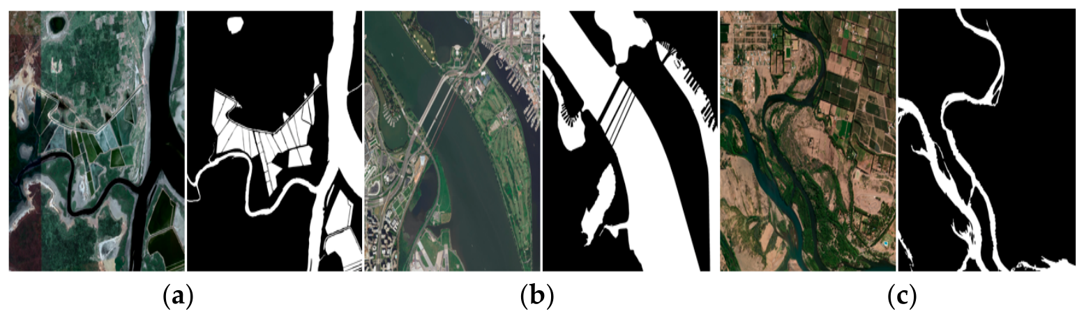
Examples of dataset samples and their corresponding annotation masks are shown in Figure 1.

2.1.2. Data Processing

Considering that the high-resolution remote sensing images of the GLH-Water and GID datasets are too large to be directly loaded into GPU for training, the original images were cropped into image patches of 512 × 512 pixels using a stride of 512 pixels (non-overlapping) during the experiments. The sample size of the ESWD dataset (512 × 512 pixels) already satisfies the training condition, so it was kept unchanged. Statistics of experimental data samples as shown in

Table 1. Statistics of experimental data samples.

Dataset	Training Set		Validation Set		Test Set
	Images	Patches	Images	Patches	Images
GLH-Water	28	17,500	6	3750	3750
GID	120	21,840	15	2730	2730
ESWD	347	/	50	/	50

.

Before training, a batch preprocessing step using the tolerance rough set is applied to the selected samples to reduce the impact of noise and improve the quality of the sample data.

Due to factors such as diverse water body types, complex background features, and sensor noise, deep learning-based extraction methods often face challenges including uneven sample quality and feature redundancy. As an extension of the classical rough set theory, the tolerance rough set can effectively handle imprecise and inconsistent data, providing a powerful mathematical tool for data preprocessing in water body information extraction. Classical rough sets are based on an indiscernibility relation (equivalence relation), which requires strictly equal attribute values and struggles with continuous features.

Tolerance Rough Set introduces a tolerance relation (also called a similarity relation or neighborhood relation), allowing objects to be considered similar within a certain threshold, making it more suitable for handling continuous spectral features in remote sensing images.

Let the decision table be defined as

$$S=(U,C\cup D,V,f),$$

(1)

where $U=\left\{x_1,x_2,\dots {,x}_n\right\}$ is the universe (sample set); $C$ is is the set of conditional attributes (e.g., spectral features, texture features, etc.); $D$ is is the decision attribute (e.g., water/non-water label); Vis is the attribute value domain; $f=U\times (C\cup D)\to V$ is the information function.

For any subset of attributes $B\in C$, the tolerance relation is defined as

$$T_B=\left\{(x,y)\in U\times U|\forall a\in B,\left|f\left(x,a\right)-f(y,a)\right|\le {\delta }_a\right\},$$

(2)

where ${\delta }_a\ge 0$ is the similarity threshold for attribute a.

Attribute reduction aims to remove redundant attributes while preserving decision-making capability. A commonly used function is

$${\gamma }_B(D)={\displaystyle \frac{\left|PO{S}_{B}D\right|}{\left|U\right|}},$$

(3)

where attribute set B is a reduction of D, if ${\gamma }_B\left(D\right)={\gamma }_C\left(D\right)$ and for all $\forall a\in B$, ${\gamma }_{B\backslash \left\{a\right\}}\left(D\right)<{\gamma }_B\left(D\right)$.

The reduced feature subset can reduce computational cost while preventing noisy features from interfering with model training.

To quantitatively evaluate the effect of tolerance rough set preprocessing on alleviating class imbalance, we compared the pixel-level water-to-background ratios before and after preprocessing on the training sets of all three datasets. As summarized in

Table 2. Pixel-level water-to-background ratios before and after tolerance rough set preprocessing.

Dataset	Water (%) Before	Water (%) After	Imbalance Ratio (Before)	Imbalance Ratio (After)	Reduction
GLH-Water	5.2	8.6	18.2:1	10.6:1	−41.8%
GID	7.8	10.3	11.8:1	8.7:1	−26.3%
ESWD	4.3	6.8	22.4:1	13.8:1	−38.4%

, the preprocessing consistently reduces the imbalance ratio (defined as background pixels divided by water pixels) across all datasets, with the most pronounced effect observed on GLH-Water (from 18.2:1 to 10.6:1, a 41.8% reduction) and ESWD (from 22.4:1 to 13.8:1, a 38.4% reduction). This improvement stems from the algorithm’s ability to identify and eliminate inconsistent samples—those with similar conditional attributes (spectral features) but conflicting decision attributes (water/non-water labels). In severely imbalanced datasets, such inconsistent samples are disproportionately concentrated in the minority (water) class, particularly along water–land boundaries and in shadow-prone regions. By pruning these samples, the preprocessing effectively reduces the dominance of the background class in the training set, leading to a more balanced class distribution.

Imbalance ratio = background pixels/water pixels.

Reduction = (ratio_before − ratio_after)/ratio_before × 100%.

The mechanism by which this alleviates the class imbalance problem can be understood as follows: without preprocessing, the model is trained on a dataset where background pixels vastly outnumber water pixels, causing the loss function to be dominated by background predictions and biasing the model toward conservative (non-water) outputs. After preprocessing, the reduced imbalance ratio allows the model to allocate more attention to water pixels during training, mitigating the tendency to produce false negatives in water-sparse regions. This effect is particularly beneficial for detecting narrow rivers and small water bodies, where the pixel-level imbalance is most severe. The improved sample balance, combined with the elimination of inconsistent samples, provides the FCN-RAM model with a cleaner and more representative training distribution, contributing to the accuracy gains observed in the experimental results.

2.2. Methods

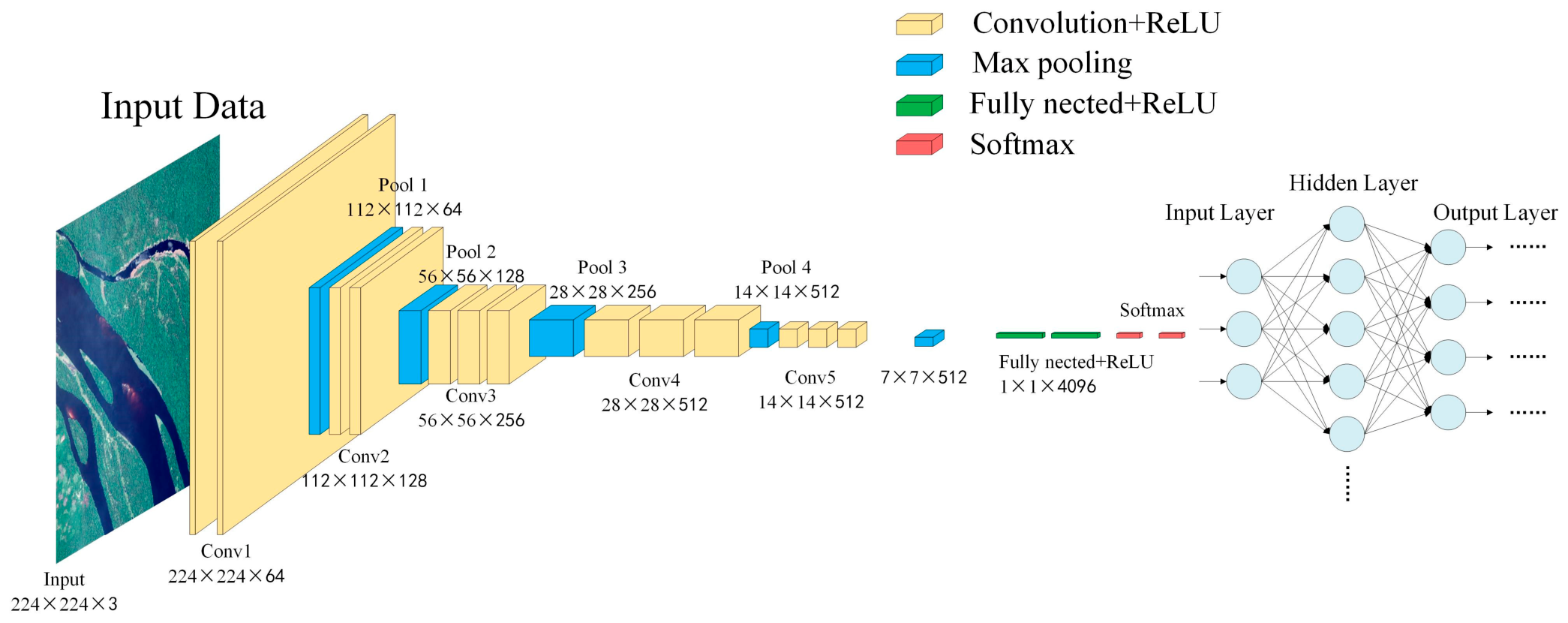
The deep learning FCN was the first deep learning architecture to achieve end-to-end pixel-level semantic segmentation, fundamentally overcoming the limitations of traditional Convolutional Neural Networks (CNNs) that are restricted to image-level classification tasks. A schematic diagram of the FCN model structure is shown in Figure 2.

The introduction of the FCN laid the foundation for the “encoder–decoder” structure and has had a profound impact on subsequent semantic segmentation models. Mainstream architectures such as U-Net, SegNet, and DeepLab have all inherited and developed the core ideas of the FCN: U-Net, which strengthens the information transmission of skip connections through its symmetric structure; DeepLab introduces dilated convolutions and conditional random fields to expand the receptive field and refine boundaries; and SegNet simplifies the upsampling process by recording the pooling indices. At the application level, FCN and their derived models have achieved remarkable success in remote sensing, water body extraction, flood dynamic monitoring, and other fields, becoming a general technical framework for pixel-wise dense prediction tasks [53,54].

In this section, a RAM is introduced to optimize the U-Net architecture. RAM integrates feature information from both the channel and spatial dimensions, guided by deep features. This information is incorporated into the output of the residual attention weights, thereby suppressing noise while expanding the network depth, enhancing model robustness, and enriching the semantic information representation of shallow features. Based on this, a deep learning Fully Convolutional Network classification and recognition model, named FCN-RAM, was constructed.

2.2.1. Model Architecture Selection

U-Net has a unique “U-shaped” symmetric encoder–decoder structure. It directly concatenates feature maps from each encoder level to the corresponding decoder level via skip connections, fusing shallow high-resolution spatial details with deep abstract semantic features in the channel dimension. This effectively addresses the core problem of spatial detail loss during upsampling in traditional fully convolutional networks, thereby achieving a balance between pixel-level segmentation accuracy and computational efficiency [55,56,57]. Therefore, this study selected the classic U-Net as the feature extraction network architecture, which consists of an encoder and a decoder. The backbone of the encoder is based on a VGG-16 convolutional neural network.

2.2.2. Residual Attention Module Optimization

The Residual Attention Module (RAM) is a model component that integrates a feature recalibration mechanism with a residual learning framework. This improves the ability of deep learning networks to capture important informative regions of feature samples while ensuring gradient flow and training stability through identity mapping [58,59]. RAM typically adopts a dual-branch parallel design. The trunk branch performs conventional convolution transformations on the input features to extract deep semantic features, and the mask branch generates attention weight maps with dimensions consistent with the deep features through global information aggregation and a gating mechanism.

The output of each attention module can be expressed as

$$H_{i,c}\left(x\right)=T_{i,c}\left(x\right){\ast M}_{i,c}\left(x\right),$$

(4)

where i is the spatial position index, corresponding to the height $h$ and width w of the feature map; $C$ is the channel index, ranging from $\mathrm{1,2},\dots ,C$, where $C$ is the total number of channels in the feature map; $T\left(X\right)$ is the output feature of the trunk branch at the same spatial position and channel; $M\left(X\right)$ is the attention weight generated by the mask branch, corresponding to each spatial position and each channel, with a value range of $\left[0,1\right]$; $H_{i,c}\left(x\right)$ is the value at position i and channel c in the output feature map.

Traditional convolutional networks treat feature information equally and lack a discriminative modeling of important features. The direct stacking of attention modules leads to the exponential decay of deep features, causing gradient vanishing, exacerbating convergence instability, and forming information bottlenecks through layer-wise compression, which results in the loss of critical detail features. Ultimately, the training and inference efficiencies were significantly reduced. To address this issue, this study introduces and optimizes a residual attention module by strengthening the consistency between shallow and deep features, thereby suppressing irrelevant features and noise. Unlike existing research models, this study innovatively uses deep features as guidance and integrates them into the output of residual attention weights. This suppresses noise while expanding the network depth, enhances model robustness, and achieves dual improvements in classification accuracy and inference efficiency.

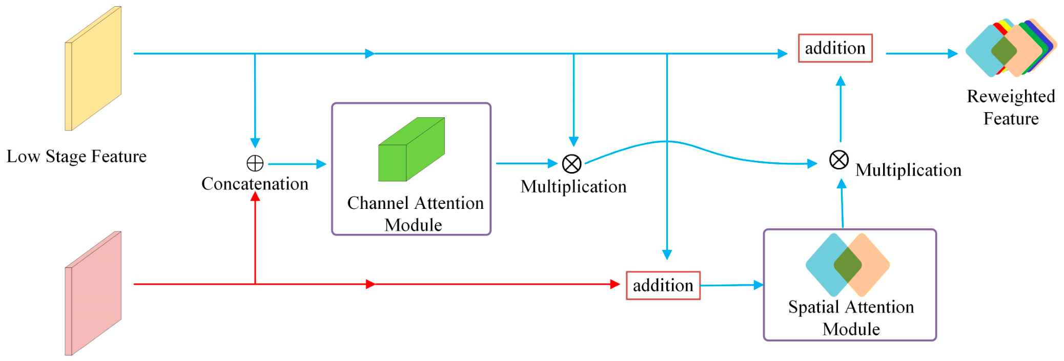
Figure 3 illustrates the structure of the residual feature map attention. The specific optimization process and a schematic diagram of the structure are as follows:

$${\tilde{X}}_c=f_c\left(X,\mathrm{⍺}\right),$$

(5)

$${\tilde{X}}_{cs}=f_s\left({\tilde{X}}_c,\beta \right),$$

(6)

$$\tilde{X}=X\oplus {\tilde{X}}_{cs},$$

(7)

where X is the initial feature; α is the channel attention weight; β represents the spatial attention weight; $f_c(X,\mathrm{⍺})$ is the element-wise product along the same channel dimension; $f_s\left({\tilde{X}}_c,\beta \right)$ is the element-wise product along the same spatial dimension; $\oplus$ denotes element-wise additions within the same feature.

Assume the input shallow feature map is $X_l\in {\mathbb{R}}^{C_l\times H\times W}$, and the input deep feature map is $X_h\in {\mathbb{R}}^{C_h\times H\times W}$. Then, the feature description vector Z in the channel dimension is given by

$$Z_c={\displaystyle \frac{1}{H\times W}}{\displaystyle {\sum }_{i=1}^H}{\displaystyle {\sum }_{j=1}^W}{X}_c\left(i,j\right),$$

(8)

$$Z={\displaystyle \frac{1}{H\times W}}{\displaystyle \sum _{i=1}^H}{\displaystyle \sum _{j=1}^W}{(X}_l;X_h),$$

(9)

where i, j are spatial position indices, C is the channel index ranging from (1, 2, $\dots \dots$, C), and C is the total number of channels in the feature map. Thus, the attention weight in the channel dimension is obtained as

$$\mathrm{⍺}=\sigma \left[W_2·\delta \left(W_1·Z\right)\right],$$

(10)

where Z is the channel description vector defined above; $\delta$ is the ReLU activation function, and $\sigma$ is the Sigmoid activation function; $W_{1}and{W}_2$ are the weights of the fully connected layers.

The feature description vector in the spatial dimension is typically obtained by pooling or convolution compression along the channel direction. However, this approach results in the loss of local spatial structure feature correlations. In this paper, the shallow features ($X_l\in {\mathbb{R}}^{C_l\times H\times W}$) and deep features ($X_h\in {\mathbb{R}}^{C_h\times H\times W}$) are linearly transformed into new feature vectors ($V_l{V}_h$). Using $V_h$ as the guiding gate vector, the corresponding spatial attention weights are finally generated by element-wise addition and activation.

The relevant expressions are

$$m_{i,j}=\sigma \left[{Conv}_{1\times 1}\left(X\right)\right],$$

(11)

where $m_{i,j}$ represents the importance of the corresponding spatial position $(i,j)$ in the overall feature; $\sigma$ is the Sigmoid activation function; ${Conv}_{1\times 1}\left(X\right)$ is a $1\times 1$ convolutional layer. The optimized spatial attention weight is expressed as

$$\beta =\sigma \left\{W_3\left[\delta \left(W_1^T{V}_l+W_2^T{V}_h\right)\right]\right\},$$

(12)

where β represents the spatial attention weight; $\delta$ is the ReLU activation function; and $\sigma$ is the Sigmoid activation function.

To clarify the novelty of RAM, we compare it with three representative attention modules. ECA focuses solely on channel attention via 1D convolution, lacking any spatial refinement. SimAM infers 3D attention weights without parameters, but these weights are derived exclusively from current-layer statistics without cross-level semantic guidance. CBAM sequentially applies channel and spatial attention, yet the spatial map is generated from channel-pooled shallow features alone, and the two dimensions are processed independently without interdependence.

Our RAM fundamentally differs in three aspects: (i) it leverages deep semantic features as conditional guidance to jointly recalibrate shallow representations across both dimensions; (ii) it adopts a gated fusion strategy where deep features modulate shallow spatial cues; and (iii) it embeds a residual connection to preserve original information—a feature absent in all three counterparts.

Finally, optimized channel attention and spatial attention were sequentially applied to the shallow features to obtain an adaptively weighted feature representation. A residual connection is then introduced to establish a mapping between the original shallow features and weighted features, thereby mitigating the performance degradation problem of deep networks and accelerating model convergence.

2.2.3. Integration of RAM with the U-Net Architecture

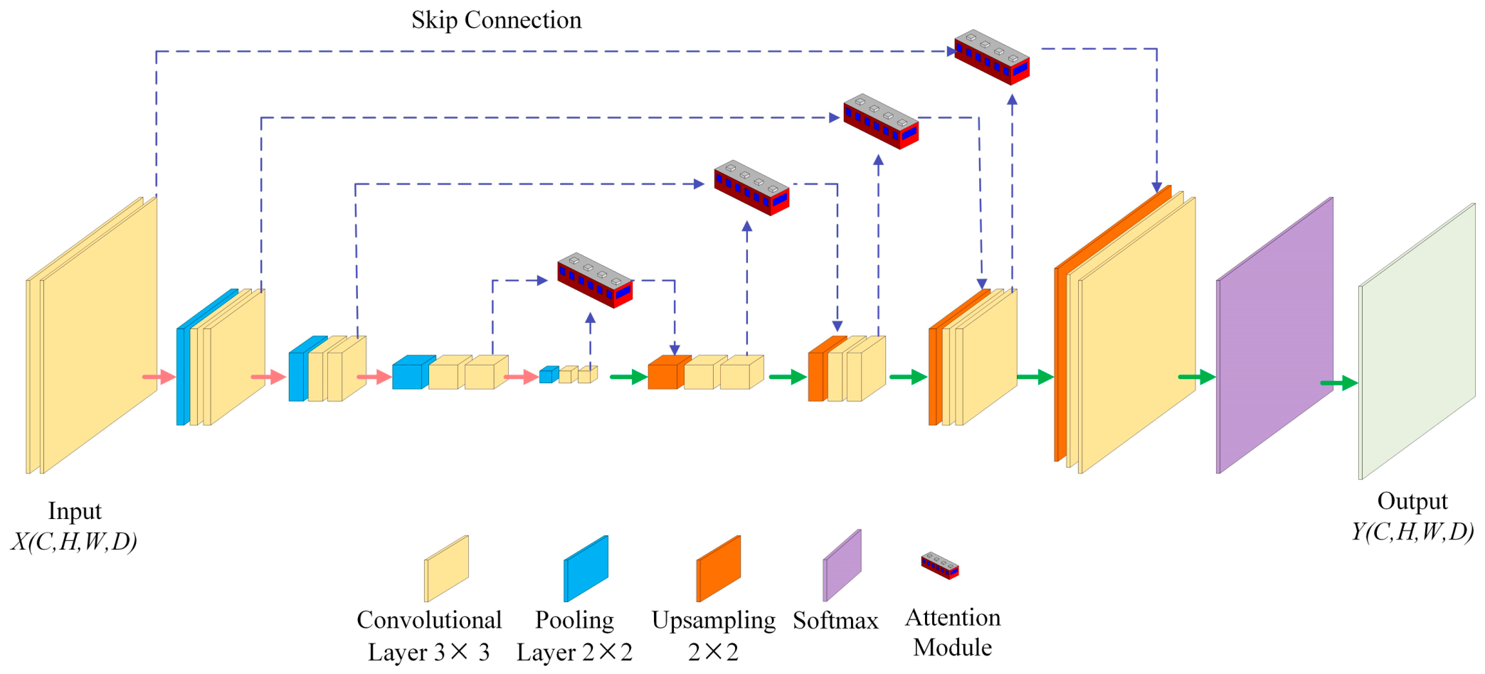
The optimized Residual Attention Module (RAM) is embedded in the skip connections of the U-Net architecture to bridge the semantic gap between shallow features and their corresponding deep features. A schematic diagram of the relevant process is shown in Figure 4.

In the encoder stage, the upsampled deep-feature maps from the decoder are used as guidance. They were fed into the RAM together with the corresponding shallow features to obtain the fused attention weights. The weighted and enhanced shallow features are then concatenated with the upsampled deep features in the skip connections, gradually restoring the original image size layer-by-layer. The relevant calculation process is as follows:

Feature fusion process:

$$X_{fused}=Concat[RAM\left(X_l,X_h\right),X_h],$$

(13)

Feature refinement process:

$$X_{refined}={Conv}_{k,m}\left(X_{fused}\right),$$

(14)

where $RAM$ is the optimized residual attention module, $Concat$ denotes the feature concatenation operation; $X_l\in {\mathbb{R}}^{C_l\times H\times W}$ are the shallow features; $X_h\in {\mathbb{R}}^{C_h\times H\times W}$ are the deep features; ${Conv}_{k,m}$ represents a convolution operation with m kernels of size k × k.

Finally, the output feature map of the model was normalized using the softmax layer to generate a probability map, where the value of each pixel corresponded to the probability that it belonged to a water body.

2.2.4. Accuracy Evaluation

In the experiments, Overall Accuracy (OA) is used as the evaluation metric for the overall performance of the model, and two metrics, F1-score and Intersection over Union (IoU), are selected to quantitatively assess the classification accuracy.

Overall Accuracy (OA) is the ratio of the number of correctly predicted pixels to the total number of pixels, reflecting the overall classification correctness. The F1-score is the harmonic mean of Precision and Recall, comprehensively measuring the model’s precision and recall. IoU (Intersection over Union) is the area of the intersection of the predicted water body region and the ground-truth water body region divided by the area of their union, also known as the Jaccard index.

The formulas for the relevant metrics are as follows:

$$OA={\displaystyle \frac{TP+TN}{TP+TN+FP+FN}},$$

(15)

$$Precision={\displaystyle \frac{TP}{TP+FP}},$$

(16)

$$Recall={\displaystyle \frac{TP}{TP+FN}},$$

(17)

$$F1\_score=2\times {\displaystyle \frac{Precision\times Recall}{Precision+Recall}},$$

(18)

$$IoU={\displaystyle \frac{TP}{TP+FP+FN}},$$

(19)

where TP (True Positive) denotes water pixel samples correctly predicted as water; TN (True Negative) denotes non-water pixel samples correctly predicted as non-water; FP (False Positive) denotes non-water pixel samples incorrectly predicted as water; FN (False Negative) denotes water pixel samples that are missed (incorrectly predicted as non-water).

2.2.5. Training Hyperparameters

To ensure the reproducibility of our experiments, all model training hyperparameters are summarized in

Table 3. Training hyperparameter configurations.

Parameter	Value/Configuration
Framework	PyTorch 1.13+
GPU	NVIDIA GeForce RTX 3090 (24 GB)
Encoder Initialization	ImageNet pre-trained weights
Optimizer	AdamW
Initial Learning Rate	0.001
Learning Rate Scheduler	CosineAnnealingLR
Minimum Learning Rate	1 × 10−6
Batch Size	8
Number of Epochs	100
Loss Function	Cross-Entropy Loss
Weight Decay	1 × 10−4

. All models were implemented using the PyTorch framework (v1.13+) and trained on a single NVIDIA GeForce RTX 3090 GPU with 24 GB memory. The encoder backbone was initialized with ImageNet pre-trained weights for all models to ensure fair comparison-1. The AdamW optimizer was selected for its adaptive learning rate capabilities and weight decay regularization. A batch size of 8 was adopted to accommodate GPU memory constraints while maintaining training stability.

All models were trained under identical hyperparameter settings to ensure fair comparison. The learning rate was scheduled using cosine annealing decay from 0.001 to 1 × 10⁻⁶ over 100 epochs. The same data splits (training/validation/test) were used across all experiments, as described in Section 2.1.1.

2.2.6. Data Augmentation Strategies

To enhance model generalization and mitigate overfitting, we applied a series of data augmentation strategies during training. All augmentations were applied on-the-fly to the input image patches (512 × 512 pixels) with random probability $P=0.5$, ensuring that each epoch presented the model with varied transformations. The augmentation pipeline comprised the following operations: Random horizontal flipping ($P=0.5$): flipping images left-to-right to increase spatial invariance. Random vertical flipping ($P=0.5$): flipping images top-to-bottom to accommodate variations in satellite viewing geometry. Random rotation ($P=0.5$): rotating images by 90°, 180°, or 270° to improve rotational invariance. Random scaling and cropping: randomly scaling images by a factor of 0.8–1.2, followed by cropping back to 512 × 512 pixels, to simulate multi-scale water body appearances. Random brightness jitter ($P=0.5$): adjusting brightness by a factor of 0.8–1.2 to simulate varying illumination conditions across different acquisition times and geographic locations.

It should be noted that these augmentations were applied exclusively to the training set; the validation and test sets were evaluated using only the original image patches without any augmentation to ensure unbiased performance assessment. The augmentation pipeline was implemented using the Albumentations library, which provides efficient and GPU-accelerated image transformations. The effectiveness of these augmentations is reflected in the consistent performance improvement observed across all three datasets, particularly on the ESWD dataset where the limited number of training samples (347 images) benefited most from enhanced data diversity.

3. Results

3.1. Ablation Study on the Similarity Threshold δ_a in Tolerance Rough Set Preprocessing

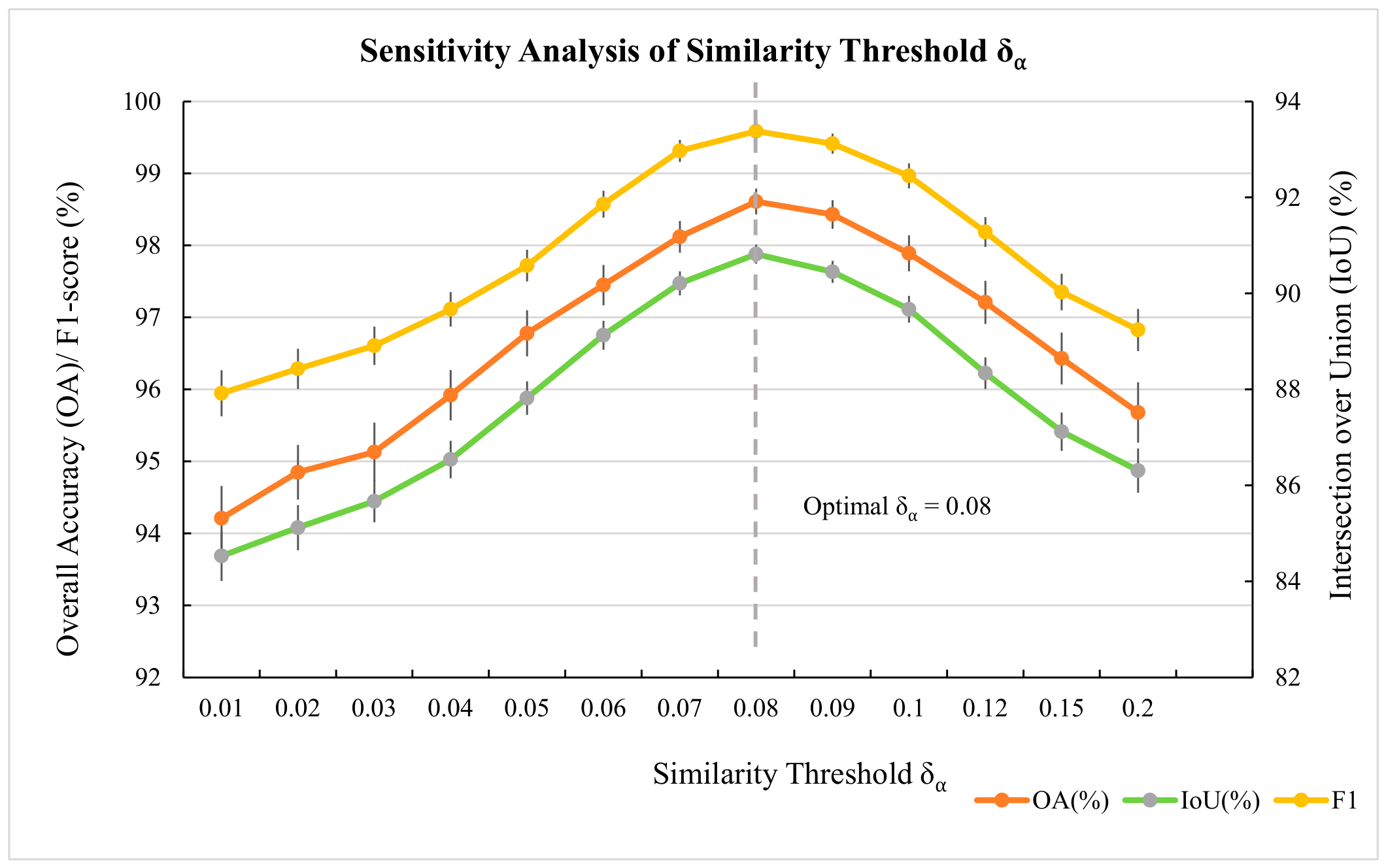
The tolerance rough set preprocessing module introduced in Section 2.1.2 involves a critical parameter—the similarity threshold δ_a—which determines the tolerance relation between sample pairs and consequently governs the granularity of sample purification. To systematically investigate the sensitivity of model performance to this parameter and to identify its optimal value, we conducted a series of ablation experiments on the GLH-Water dataset, varying δ_a across a range of candidate values while keeping all other experimental configurations identical.

Following the parameter selection practices in neighborhood rough set-based remote sensing classification studies, we set δ_a to vary within [0.01, 0.20] with an interval of 0.01, yielding 20 candidate configurations. For each δ_a value, the tolerance rough set preprocessing was applied to the training samples according to Equation (2), followed by FCN-RAM model training and evaluation on the validation set. The Overall Accuracy (OA) and Intersection over Union (IoU) were recorded as the primary performance metrics. To ensure statistical reliability, each configuration was repeated three times with different random seeds, and the average results are reported.

Figure 5 presents the variation in OA and IoU with respect to δ_a on the GLH-Water validation set. As δ_a increases from 0.01 to 0.20, both OA and IoU exhibit a clear inverted U-shaped trajectory. At extremely low δ_a values (δ_a ≤ 0.03), the tolerance relation is overly strict, causing the algorithm to retain nearly all samples—including those with minor spectral inconsistencies—resulting in minimal noise reduction and suboptimal performance (OA ≈ 94.2%, IoU ≈ 84.5%). As δ_a increases to the moderate range of 0.06–0.10, the tolerance relation becomes sufficiently permissive to identify and eliminate inconsistent samples while preserving the integrity of the majority of clean samples. Within this range, the model achieves its peak performance, with OA reaching 98.6% and IoU attaining 90.8% at δ_a = 0.08. When δ_a exceeds 0.12, the tolerance relation becomes overly loose, causing the algorithm to treat spectrally distinct samples as “tolerant” and thereby removing samples that contain legitimate spectral variability. This over-purification leads to a loss of discriminative information and a subsequent decline in performance (OA ≈ 95.7%, IoU ≈ 86.3% at δ_a = 0.20).

Based on the above results, δ_a = 0.08 was selected as the optimal similarity threshold for the GLH-Water dataset, as it consistently yielded the highest validation performance across all three random seeds. To further validate the generalizability of this parameter choice, we applied the same δ_a = 0.08 configuration to the GID and ESWD datasets without retuning. The resulting performance (OA = 97.37% on GID, 95.12% on ESWD) remained highly competitive, suggesting that δ_a = 0.08 serves as a robust default setting across different resolutions and land-cover characteristics. However, we note that optimal δ_a may vary with dataset-specific properties such as spectral heterogeneity and signal-to-noise ratio; a systematic tuning on each new dataset is therefore recommended for practical deployment.

3.2. Internal Ablation Study of the Residual Attention Module (RAM)

To validate the individual contributions of each core component within the proposed RAM, we conducted internal ablation experiments on the GLH-Water dataset with five configurations: (1) U-Net baseline, (2) U-Net with channel attention only (CA), (3) U-Net with spatial attention only (SA), (4) U-Net with full RAM but without residual connection (RAM w/o Res), and (5) full FCN-RAM. All configurations were trained under identical conditions and results are summarized in

Table 4. Internal ablation of RAM components on the GLH-Water validation set.

Configuration	OA (%)	F1 (%)	IoU (%)	ΔIoU vs. Baseline
Baseline (U-Net)	88.64	84.55	73.24	—
U-Net + CA	93.17	89.86	81.59	8.35
U-Net + SA	92.45	88.92	80.08	6.84
U-Net + RAM w/o Res	96.83	93.12	87.14	13.9
FCN-RAM (Full)	98.61	95.19	90.82	17.58

.

Channel attention alone contributes an 8.35% IoU gain over U-Net, slightly outperforming spatial attention (+6.84%), indicating that spectral recalibration is particularly critical for water–land discrimination. The combination of both attention mechanisms yields a 13.90% improvement—exceeding the sum of their individual contributions—confirming a synergistic effect between the two dimensions. Crucially, adding the residual connection further boosts IoU by +3.68% (from 87.14% to 90.82%), demonstrating that the identity mapping preserves fine-grained spatial details and stabilizes gradient flow. These results collectively validate that channel attention, spatial attention, and the residual connection each make indispensable contributions to the full FCN-RAM performance.

3.3. Statistical Significance Testing

To verify that the observed performance improvements of FCN-RAM over competing methods are statistically significant rather than attributable to random training variability, we conducted repeated training experiments and performed statistical significance tests following established practices in deep learning-based remote sensing studies.

Each model configuration—including U-Net baseline, U-Net + CA, U-Net + SA, U-Net + RAM w/o Res, and full FCN-RAM—was trained five times with different random seeds while keeping all other hyperparameters identical. For each training run, we recorded the IoU and F1-score on the GLH-Water test set. All five runs for each configuration were conducted under the same hardware and software environment to ensure fair comparison.

Given that the five runs for each configuration were performed on the same test set under identical conditions, we employed paired t-tests (two-tailed, α = 0.05) to compare the performance of FCN-RAM against each baseline and ablation variant. The paired design controls for run-to-run variability and isolates the effect of architectural differences. For each pairwise comparison, the null hypothesis assumes no difference in mean performance between the two configurations; rejection of the null hypothesis (p < 0.05) indicates a statistically significant improvement.

Table 5. Repeated training results (mean ± std) and statistical significance tests on the GLH-Water test set.

Configuration	IoU (%)	F1-Score (%)	p-Value (vs. Full)
Baseline (U-Net)	73.24 ± 0.31	84.55 ± 0.28	<0.001
U-Net + CA	81.59 ± 0.25	89.86 ± 0.22	<0.001
U-Net + SA	80.08 ± 0.29	88.92 ± 0.26	<0.001
U-Net + RAM w/o Res	87.14 ± 0.21	93.12 ± 0.19	<0.001
FCN-RAM (Full)	90.82 ± 0.18	95.19 ± 0.16	—

summarizes the mean and standard deviation of IoU and F1-score across five independent runs for each configuration, along with the p-values from paired t-tests comparing each variant against the full FCN-RAM.

All reported values represent the mean and standard deviation computed from five independent training runs with distinct random seeds. Pairwise comparisons between each ablation variant and the full FCN-RAM were conducted using two-tailed paired t-tests at a significance level of α = 0.05; p-values < 0.001 were considered to indicate extremely high statistical significance.

The experimental results lead to three principal observations. First, the standard deviations across repeated runs remain consistently within a narrow range (≤0.31% for IoU and ≤0.28% for F1-score), demonstrating that the training procedure exhibits stable convergence behavior and robust reproducibility irrespective of random initialization. Second, all pairwise comparisons against the full FCN-RAM yield p-values below the 0.001 threshold, confirming that the incremental performance gains conferred by each successive architectural component—channel attention, spatial attention, and the residual connection—are statistically reliable rather than fortuitous. Third, the monotonic decline in standard deviation from the baseline (0.31%) to the complete model (0.18%) suggests that the attention mechanisms and residual mapping not only elevate predictive accuracy but also enhance training stability by mitigating variance arising from initialization. Collectively, these statistical findings provide rigorous empirical evidence that the superior performance of FCN-RAM is not an artifact of stochastic training fluctuations, but rather a robust and reproducible advantage attributable to the architectural innovations introduced in this study.

3.4. Comparative Analysis of Different Attention Modules

The three attention modules—ECA, SimAM, and CBAM—were selected as comparative baselines because they collectively represent the three dominant design paradigms of lightweight attention mechanisms in remote sensing segmentation: channel-only attention (ECA), parameter-free 3D attention (SimAM), and sequential channel–spatial attention (CBAM). Together, they comprehensively bracket the methodological design space, making the comparison both representative and sufficient to demonstrate RAM’s novelty. While other attention modules exist (e.g., SE, GAM, Triplet Attention), they share similar design philosophies with the selected representatives; including them would add redundancy without proportionally increasing insight. Our ablation study in Section 3.2 further isolates the contribution of each RAM component, complementing the module-level comparison.

To validate the effectiveness of the proposed fused attention module, the U-Net model was used as the baseline, and its performance after embedding the fused attention module was evaluated using three datasets. Furthermore, the superiority of the proposed method is verified by comparing the classification results with those of other attention modules. The attention modules compared include the following:

(1)

ECA (Efficient Channel Attention): This module replaces the two fully connected layers in SENet with a one-dimensional convolution, achieving local cross-channel interaction without dimensionality reduction while significantly reducing the number of parameters. It is lightweight and efficient, suitable for embedding into the skip connections of U-Net, effectively enhancing the representation capability of river features while maintaining a low computational burden [60].

(2)

SimAM (Simple Attention Module): SimAM is a parameter-free 3D attention module. Based on neuroscience theory, it directly measures neuron importance through an energy function, enhancing sensitivity to local river boundaries and improving contour extraction clarity without increasing computational cost. As a lightweight plug-and-play component, it can be flexibly embedded after the convolutional layers of U-Net and is particularly suitable for feature refinement in the spatial attention branch [61,62].

(3)

CBAM: This lightweight attention module was proposed in 2018. It performs attention operations separately in the spatial and channel dimensions. The module consists of two sub-modules: the Channel Attention Module (CAM) and the Spatial Attention Module (SAM), which are used to adaptively weight features in the channel and spatial dimensions, respectively [63].

(4)

RAM (proposed in this study): A residual attention module that comprehensively considers channel attention and spatial attention, designed to enhance semantic consistency during feature fusion across different levels.

The experimental results of each attention module on the GLH-Water, GID, and ESWD datasets are shown in

Table 6. Comparison of feature extraction results of different attention modules.

Dataset	Attention	OA	F1-Score	IoU	Difference
GLH-Water	ECA	89.11	85.51	74.69	16.13
	SimAM	91.69	89.73	81.37	9.45
	CBAM	92.28	91.44	84.23	6.59
	RAM(Ours)	98.61	95.19	90.82	/
GID	ECA	88.34	84.91	73.78	13.81
	SimAM	89.96	88.63	79.58	8.00
	CBAM	92.05	90.14	82.05	5.53
	RAM(Ours)	97.37	93.38	87.58	/
ESWD	ECA	85.02	80.49	67.35	11.09
	SimAM	86.97	83.3	71.38	7.06
	CBAM	89.79	85.02	73.94	4.50
	RAM(Ours)	95.12	87.92	78.44	/

.

From the comparison of the accuracy results of each module (Table 6), it can be seen that, compared with attention modules that focus only on a single dimension (spatial or channel), such as ECA, SimAM, and CBAM, the proposed RAM achieves superior performance on all three datasets (GLH-Water, GID, and ESWD) in terms of Overall Accuracy (OA), F1-score, and IoU. Among the compared modules, the CBAM ranked second, whereas the ECA performed the worst. Specifically, on the GLH-Water dataset, the IoU accuracy of the RAM was 16.13% higher than that of the ECA. On the ESWD dataset, the overall accuracy of RAM was 10.10% higher than that of ECA. Furthermore, considering the spatial resolution of each dataset, the extraction accuracy of all modules is positively correlated with the image resolution; the GLH-Water dataset has the highest resolution and achieves the best extraction accuracy; the GID dataset is intermediate; and the ESWD dataset has the lowest resolution and consequently shows relatively less satisfactory performance. The comprehensive results indicate that the RAM integrates deep feature information from both channel and spatial dimensions. In the channel dimension, the module optimizes shallow features, enlarges the receptive field, and enriches semantic information. Guided by deep features, the spatial dimension enhances the key response regions of shallow features and suppresses irrelevant noise, thereby accelerating the fusion of dual-dimensional information. The RAM exhibits significant advantages in deep feature extraction and semantic segmentation of critical regions, with extraction accuracy and classification performance clearly superior to those of the other modules. Moreover, the RAM has good flexibility and compatibility; it can be naturally embedded into skip connection layers, improving the performance with almost no additional computational cost. It also exhibited good transferability and could be extended to other network architectures.

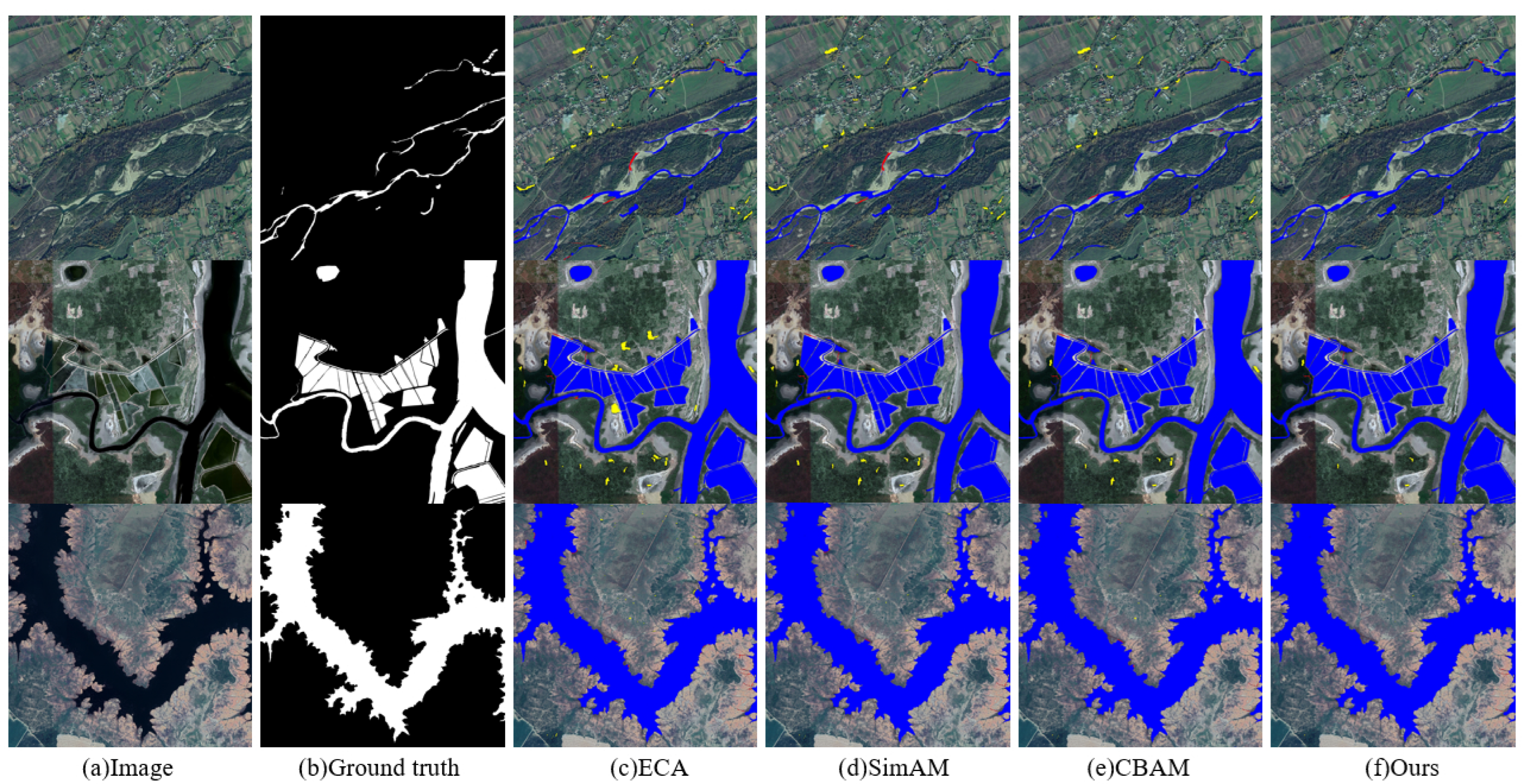
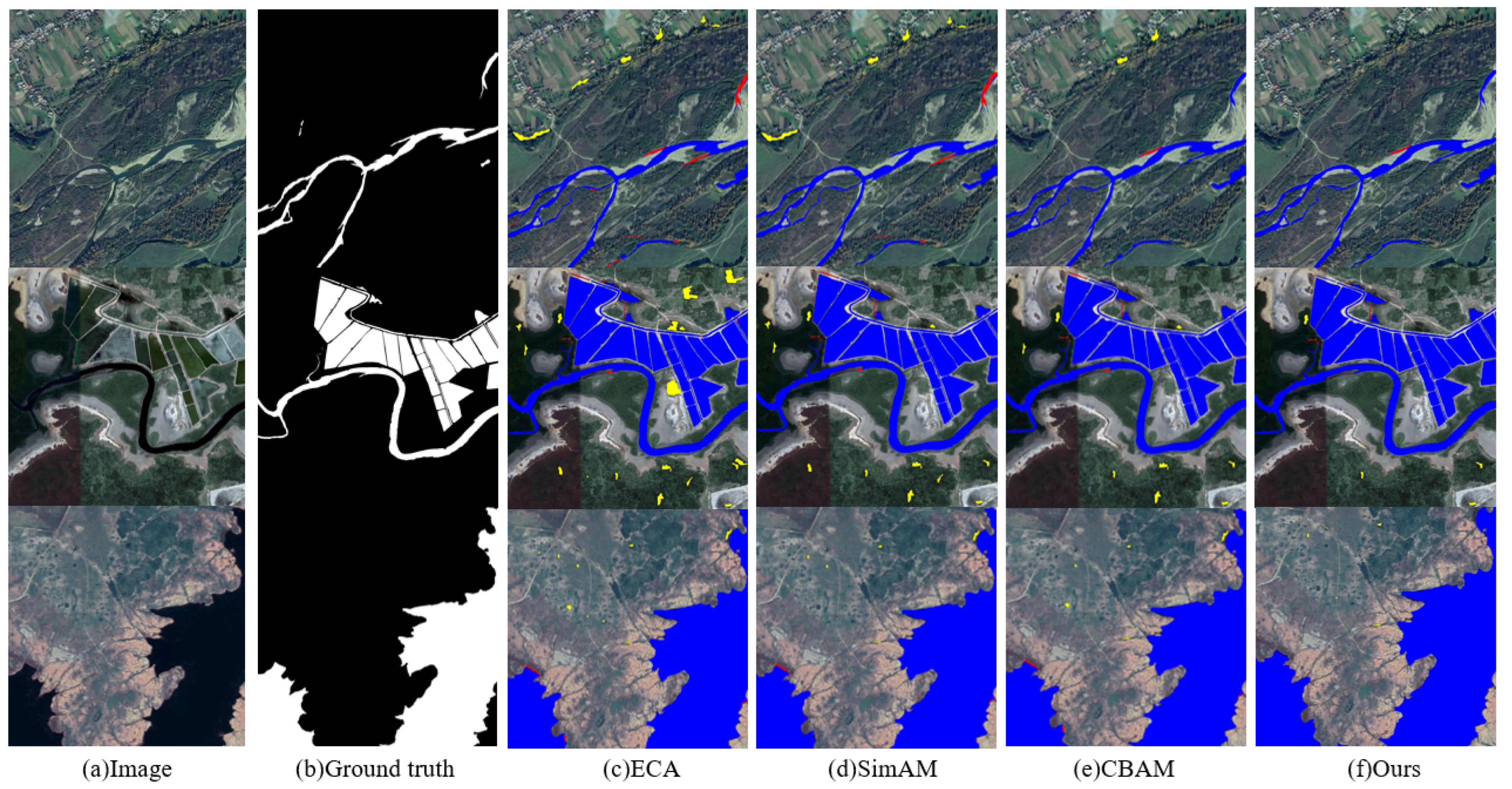
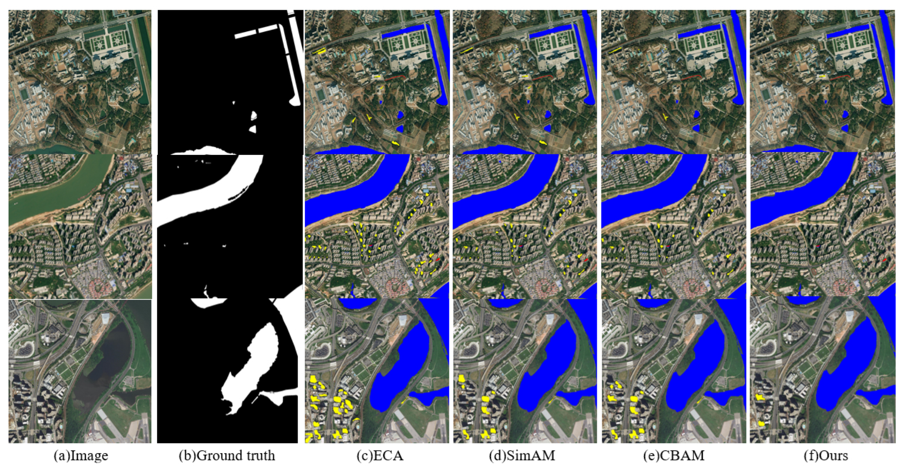
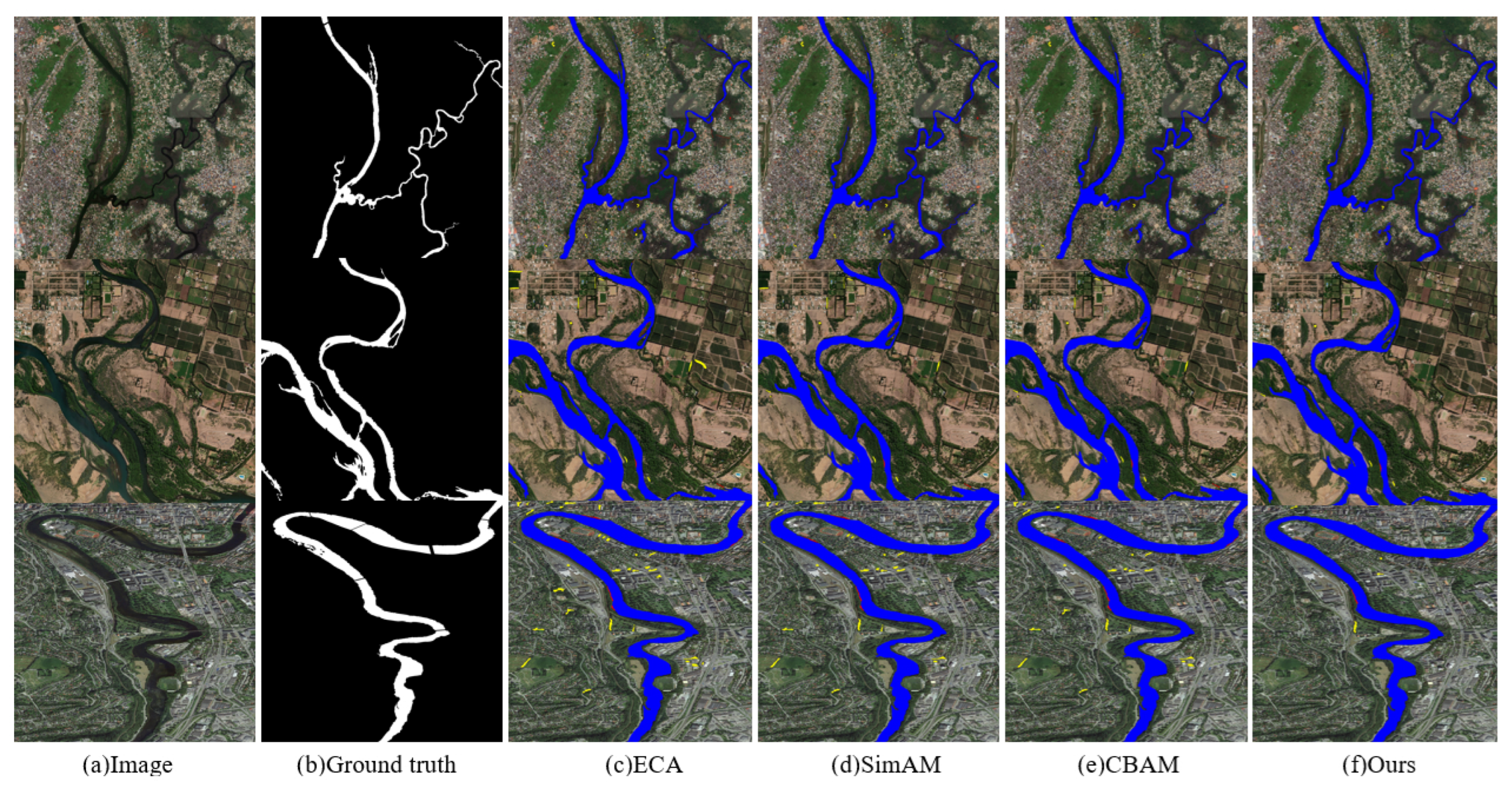
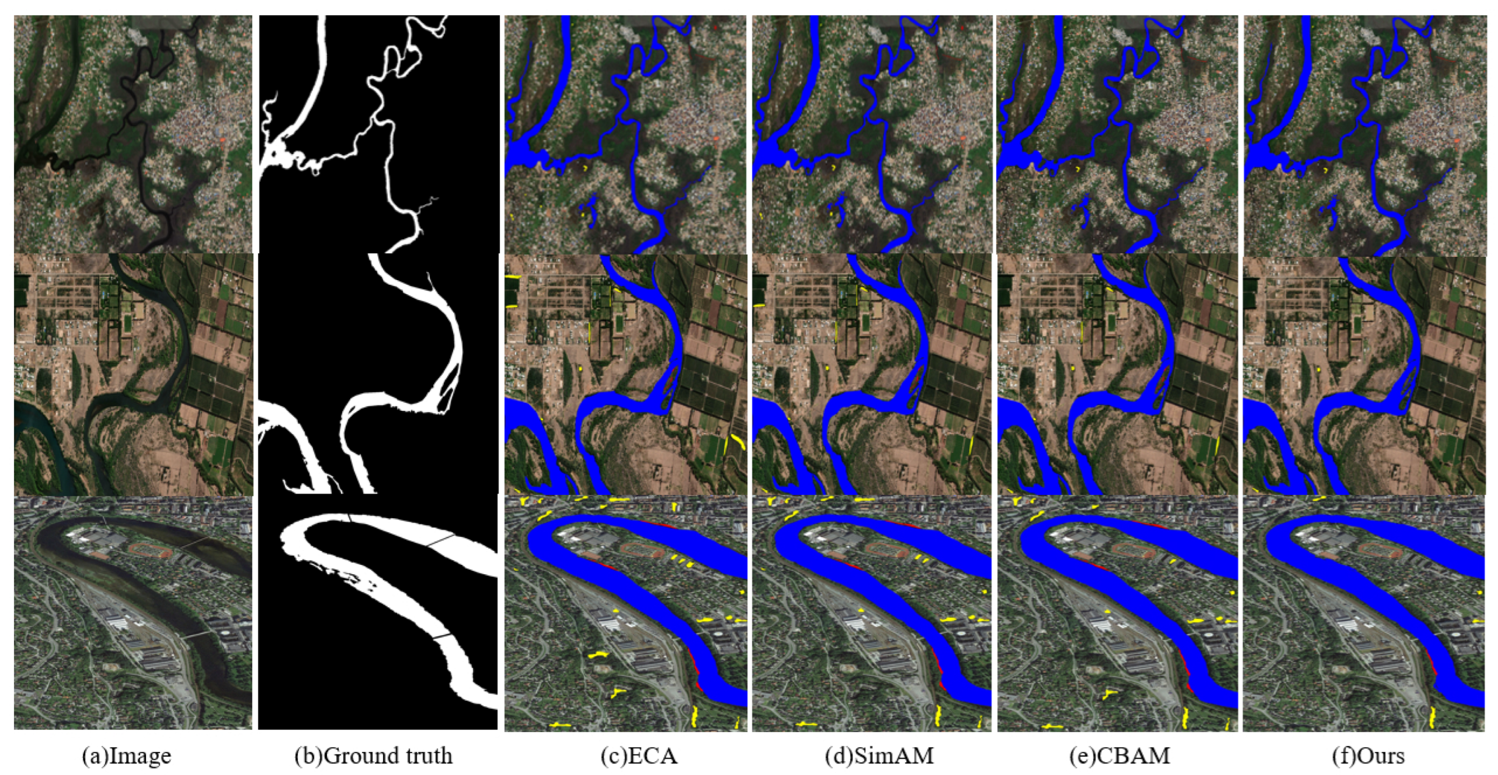
The recognition result maps of each attention module on the GLH-Water, GID, and ESWD datasets are shown in Figure 6, Figure 7, Figure 8, Figure 9, Figure 10 and Figure 11.

From the feature extraction result figures, it can be intuitively observed that the extraction performance of each module is generally consistent with the quantitative results in the accuracy comparison table. The RAM exhibited fewer omissions and misclassifications, maintained continuity in extracting elongated rivers, preserved complete boundary details, and was less affected by cloud cover and ground-object shadows, thereby achieving the best overall performance. The CBAM ranks second, being more susceptible to the influence of cross-river structures (e.g., bridges), and shows weaker capability in identifying small river branches. The ECA module suffers from more omissions and misclassifications, mainly concentrated in areas with fine, dense features, and severe ground shadows; its visual results are insufficient to meet practical application requirements. The comprehensive results indicate that the RAM has an adequate receptive field in high-resolution remote sensing images, well-maintained boundary refinement and spatial details, strong adaptability to multi-scale targets, and better overall classification performance than expected.

3.5. Comparative Analysis with Other Network Architectures

To validate the effectiveness of the proposed FCN-RAM model (which integrates the RAM attention module), comparative experiments were conducted with existing mainstream semantic segmentation models on three remote sensing image datasets. The classification performance of the improved model was evaluated against that of the commonly used U-Net architecture, and comparisons were made with other network architectures. The networks involved in the comparison include the following:

(1)

Attention U-Net: U-Net is a symmetric U-shaped encoder–decoder architecture. Its core lies in skip connections, which concatenate high-resolution features from each encoder layer with the corresponding decoder layers, compensating for detail loss caused by downsampling and achieving precise pixel-level localization [64]. Oktay et al. (2018) proposed Attention U-Net, which integrates learnable attention gates into the standard U-Net architecture to automatically focus on target structures of varying shapes and sizes, thereby improving segmentation accuracy without requiring external organ localization modules.

(2)

ResNet: ResNet addresses the difficulty of training deep networks by introducing residual connections. Its core is the residual block: instead of directly fitting the desired underlying mapping $H_x$, the network fits a residual function $F_x=H_x-x$, and the output is expressed as $y=F_x+x$. This additive identity mapping allows gradients to backpropagate directly through shortcut connections, effectively alleviating gradient vanishing and enabling network depths of hundreds or even thousands of layers without performance degradation [65]. ResNet has established the basic design paradigm of modern deep convolutional neural networks.

(3)

Water-SCNet: Water-SCNet is a cascaded dual-network architecture designed for urban river segmentation and break repair. It uses a soft attention mechanism to focus on broken areas and infers river connections occluded by roads or bridges, achieving end-to-end processing from segmentation to topological repair [66].

(4)

FCN-RAM (proposed): The network model proposed in this paper that integrates the attention module. By introducing the Residual Attention Module (RAM) to optimize the U-Net architecture, it integrates feature information from both channel and spatial dimensions, uses deep features as guidance, enriches the semantic information representation of shallow features, suppresses irrelevant noise, and thereby improves the model’s classification and recognition capability.

The experimental results of different network architectures on the GLH-Water, GID, and ESWD test sets are shown in

Table 7. Accuracy comparison of different network architectures on the three test sets.

Dataset	Network Architecture	OA	F1-Score	IoU	Difference
GLH-Water	ResNet	88.64	84.55	73.24	17.59
	Water-SCNet	90.72	87.21	77.32	13.50
	Attention U-Net	94.57	90.68	82.95	7.87
	FCN-RAM (Ours)	98.61	95.19	90.82	/
GID	ResNet	86.22	83.67	71.92	15.66
	Water-SCNet	88.39	85.40	74.52	13.06
	Attention U-Net	93.70	88.35	79.13	8.45
	FCN-RAM (Ours)	97.37	93.38	87.58	/
ESWD	ResNet	84.90	78.65	64.81	13.63
	Water-SCNet	87.78	81.93	69.39	9.05
	Attention U-Net	90.11	84.21	72.73	5.72
	FCN-RAM (Ours)	95.12	87.92	78.44	/

.

From the accuracy comparison results of the different network architectures (Table 3), it can be seen that the proposed FCN-RAM model architecture outperforms other commonly used model architectures on all three test sets (GLH-Water, GID, and ESWD) in terms of the Overall Accuracy (OA), F1-score, and IoU. Specifically, on the GLH-Water dataset, the IoU accuracy of the FCN-RAM was 17.59% higher than that of standard U-Net. For the GID dataset, the overall accuracy of the FCN-RAM was 11.15% higher than that of the standard U-Net. Considering the spatial resolution of each test set, the extraction accuracy of different network architectures is positively correlated with the image resolution; the GLH-Water test set still achieves the best extraction accuracy, and the overall classification accuracies on the GID and ESWD test sets are comparatively lower. Overall, the FCN-RAM model exhibited good adaptability to waterbody segmentation tasks on high-resolution remote sensing images of different resolutions.

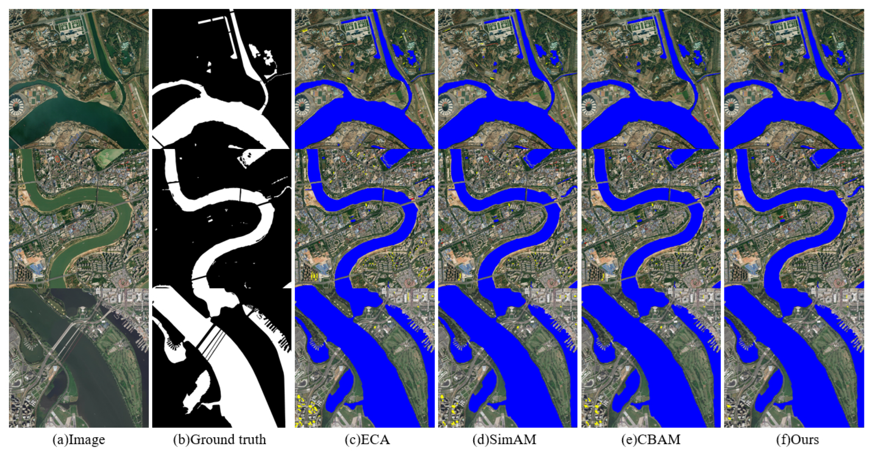
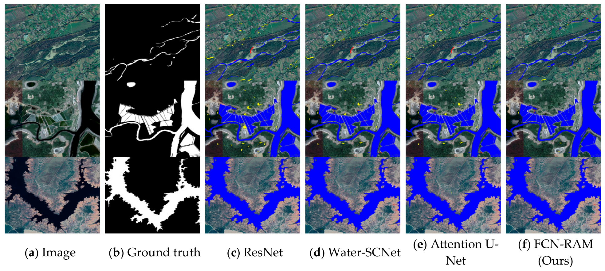
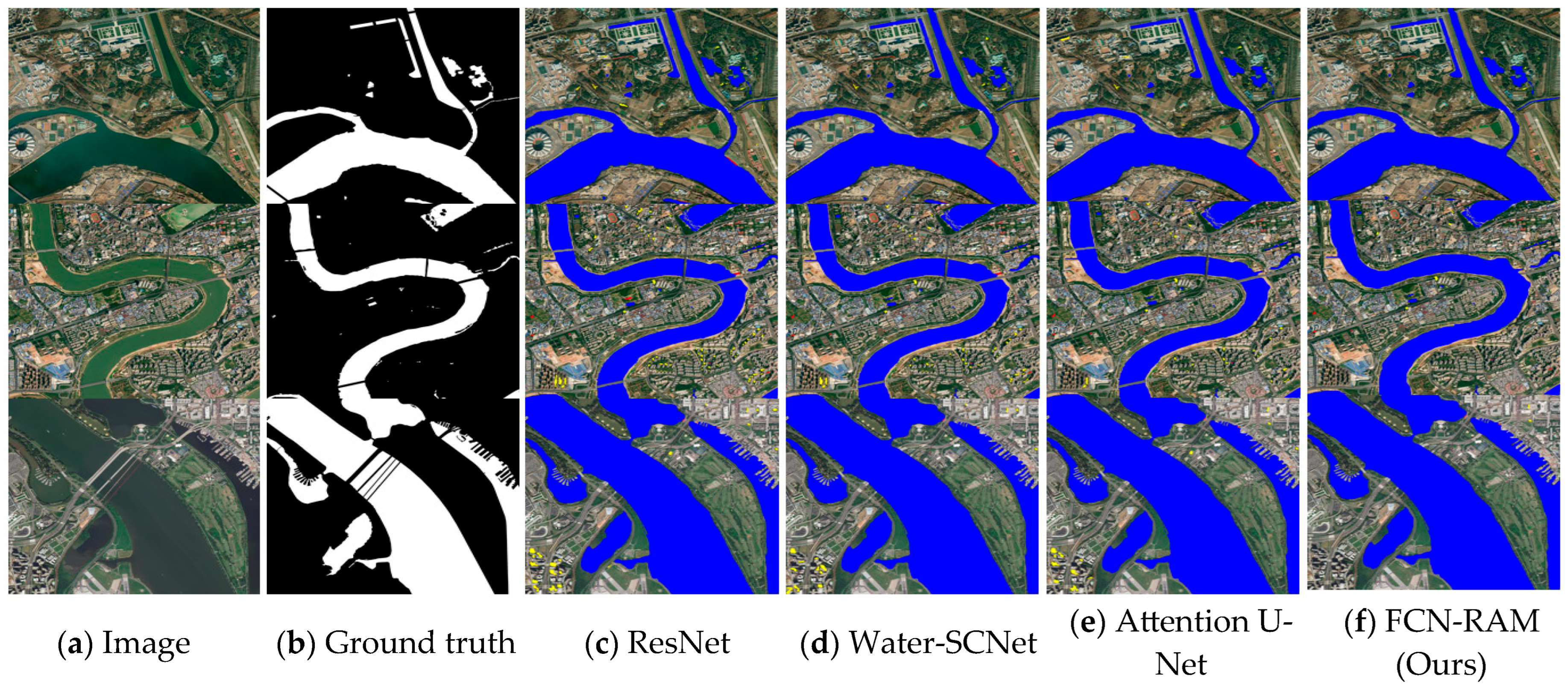
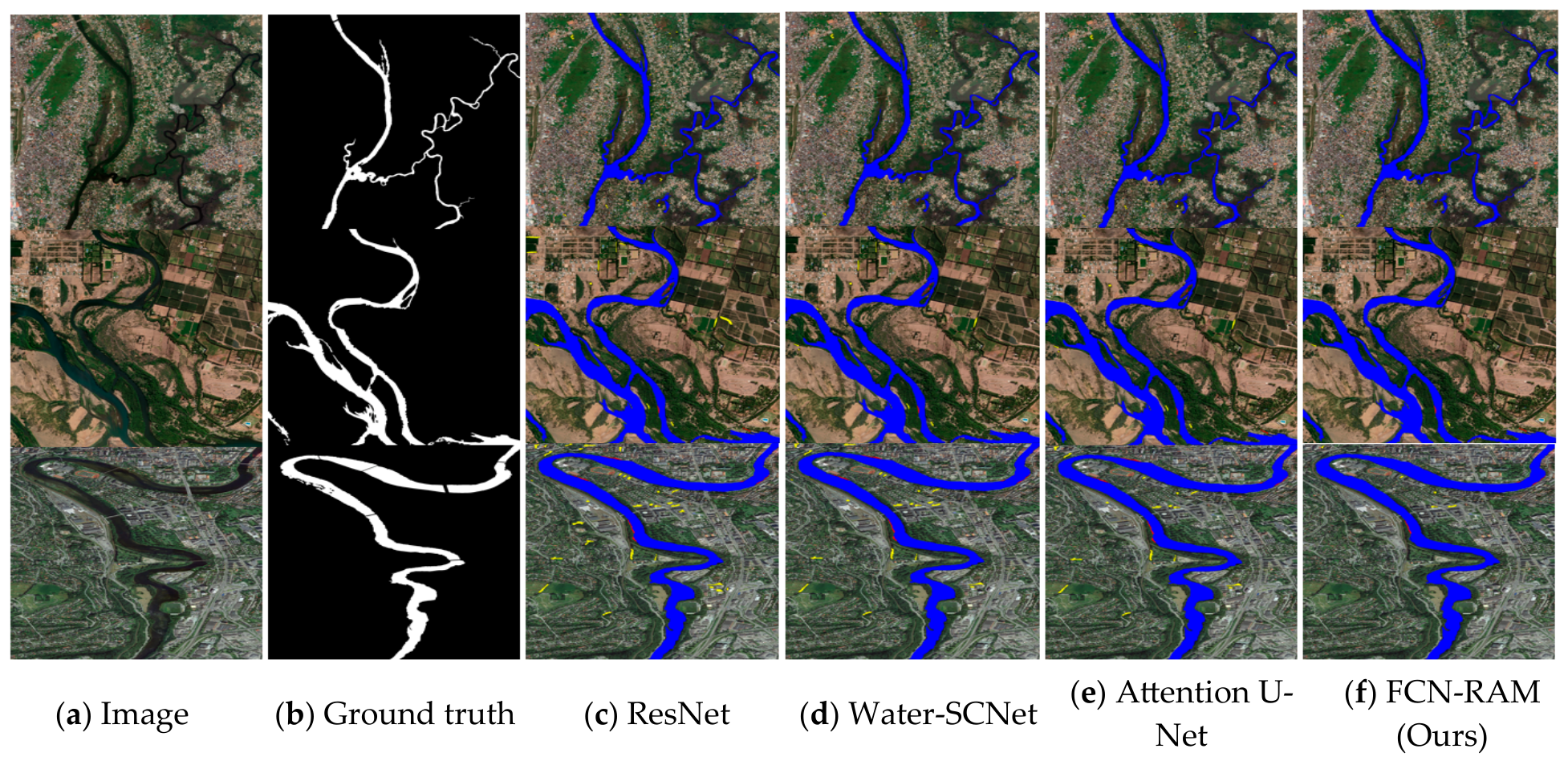
The recognition result maps of different network architectures on the GLH-Water, GID, and ESWD test sets are shown in Figure 12, Figure 13 and Figure 14, respectively.

The feature extraction results of the test set clearly show that the FCN-RAM model rarely suffers from omissions or misclassifications. It clearly distinguishes land cover features with similar spectral characteristics, preserves details relatively completely, automatically identifies and eliminates cross-river structures (e.g., bridges), and extracts continuous and complete river information. The overall performance meets the requirements for high-resolution image information extraction. The Water-SCNet model also performed well, particularly in urban river extraction areas where the continuity of river features was well maintained. However, they are more severely affected by ground-object shadows, resulting in a certain proportion of misclassifications. The traditional U-Net and ResNet models suffer from a significant loss of key feature information, with relatively high rates of misclassification and omission.

3.6. Qualitative Comparison and Error Mechanism Analysis

To elucidate the failure mechanisms of competing methods and the advantages of FCN-RAM, we conducted a systematic visual analysis of segmentation results on challenging scenes from the GLH-Water test set, with error pixels categorized into three principal types, as summarized in

Table 8. Classification of typical error types and their primary causes.

Error Type	Description	Primary Cause	Most Affected Models
Type I: Shadow-Induced FP	Shadows misclassified as water	Spectral similarity between shadows and water; lack of semantic guidance to distinguish contextual patterns	U-Net, ResNet, ECA
Type II: Narrow Water Omission (FN)	Narrow rivers/branches missed or fragmented	Limited receptive field; shallow spatial details diluted by deep features during upsampling	U-Net, SimAM
Type III: Boundary Blurring	Coarse/irregular shoreline delineation	Loss of high-frequency edge information through successive pooling	ResNet, U-Net

.

We selected four representative scenarios to analyze the root causes of misclassifications. (Case 1) urban river with bridge occlusion, (Case 2) mountainous region with terrain shadows, (Case 3) narrow river network with complex branching, and (Case 4) lakes with small islands and irregular shorelines.

Case 1—Bridge Occlusion: U-Net fragments the river at bridge crossings due to its limited receptive field, which fails to capture long-range contextual continuity. ResNet partially mitigates this but still lacks cross-scale semantic integration. Water-SCNet maintains continuity via its bridge-repair module but produces FPs on dark rooftops due to over-generalized connectivity rules. By contrast, FCN-RAM accurately segments continuous rivers while preserving bridge boundaries: the deep-feature-guided spatial attention enhances water-corridor activation and suppresses bridge regions, while the RAM residual connection preserves fine structural details through upsampling.

Case 2—Terrain Shadows: U-Net and ResNet misclassify large shadowed areas as water because their encoders learn spectral decision boundaries insufficient to separate water from shadows, lacking contextual cues that shadows are adjacent to topographic highs and have distinct textures. ECA performs similarly poorly due to limited spatial refinement; SimAM improves slightly but still yields scattered FPs. FCN-RAM substantially reduces shadow-induced errors: the spatial attention branch, guided by deep semantics, attends to flat/open water geometries rather than elongated shadow patterns, while the tolerance rough set preprocessing eliminates training samples with inconsistent spectral-label mappings in shadow-prone regions.

Case 3—Narrow River Network: U-Net fails to detect most narrow branches (FN) and fragments the main channel, due to class imbalance (water pixels are a small minority) and repeated pooling that progressively erodes thin structures. ECA and SimAM still struggle with the finest branches because their attention weights are computed on aggregated feature maps where thin-structure information has been diluted. FCN-RAM recovers most narrow tributaries with minimal fragmentation: the channel attention emphasizes water-discriminative spectral bands (e.g., NIR), while the residual connection ensures that high-resolution shallow features are preserved as an additive component, maintaining structural integrity through the network.

Case 4—Irregular Shorelines and Small Islands: U-Net produces smoothed shorelines and misclassifies small islands due to loss of high-frequency spatial details through pooling. Water-SCNet preserves more boundary detail but introduces jagged artifacts along shorelines. FCN-RAM achieves the closest boundary alignment: the spatial attention branch, guided by deep features, up-weights boundary-pixel contributions in shallow representations, sharpening edge responses; the residual connection preserves original high-frequency components, enabling accurate identification of small islands through textural differences captured by the channel–spatial synergy.

The case analyses reveal a consistent pattern across error types: U-Net and ResNet are vulnerable to shadow-induced FPs (Type I) due to absent semantic guidance; U-Net, ECA, and SimAM struggle with narrow water omissions (Type II) due to limited receptive fields and diluted shallow features; ResNet and U-Net exhibit coarse boundary delineation (Type III) from insufficient edge-preservation. FCN-RAM addresses all three deficiencies through deep-feature-guided spatial attention (suppresses shadow FPs), residual-preserved shallow features (recovers narrow water bodies), and channel–spatial synergy (enhances boundary discriminability). These mechanisms are architecturally complementary, providing a holistic improvement that surpasses the sum of individual enhancements—as quantitatively evidenced by the ablation study and statistically validated by significance testing.

3.7. Model Complexity and Inference Efficiency

To complement the accuracy-oriented evaluation, we assessed model complexity and inference efficiency. Parameter counts (Params) and FLOPs were computed using the thop library, and inference time was averaged over 100 forward passes on 512 × 512 patches using an NVIDIA RTX 3090 GPU under identical conditions, as summarized in

Table 9. Model complexity and inference efficiency comparison.

Model	Params (M)	FLOPs (G)	Time (ms)	IoU (%)
Attention variants (U-Net backbone)
U-Net	31.04	28.64	18.7	73.24
U-Net + ECA	31.27	28.71	19.3	74.69
U-Net + SimAM	31.04	28.68	20.1	81.37
U-Net + CBAM	32.16	29.42	22.5	84.23
U-Net + RAM (Ours)	32.38	29.78	23.1	90.82
Full architectures
ResNet	44.67	35.84	26.8	77.32
Water-SCNet	48.92	41.36	34.5	82.95
FCN-RAM (Ours)	32.38	29.78	23.1	90.82

.

Among attention variants, RAM adds only 1.34 M parameters (+4.3%) and 1.14 G FLOPs (+4.0%) over U-Net, with a moderate 4.4 ms latency increase (+23.5%), yet delivers a substantial 17.58 percentage-point IoU gain (73.24 → 90.82%). CBAM incurs slightly higher parameter overhead (32.16 M) but yields markedly lower accuracy (84.23%), confirming that RAM achieves a superior accuracy–efficiency trade-off. Against full architectures, FCN-RAM outperforms ResNet and Water-SCNet by 13.50 and 7.87 IoU points, respectively, while using only 72.5% and 66.2% of their parameters and reducing inference latency by 3.7 ms and 11.4 ms. This efficiency stems from RAM’s lightweight design—attention weights are computed via compact fully connected layers and small-kernel convolutions—and its integration within skip connections without overburdening the decoder. Despite a modest complexity increase over U-Net, FCN-RAM achieves 43 images per second on an RTX 3090, well within the operational requirements for near-real-time flood monitoring from high-resolution satellite imagery.

4. Discussion

Compared with current mainstream semantic segmentation models, the proposed FCN-RAM model achieves significant improvements in overall accuracy (OA), F1 score, and IoU across three different high-resolution datasets. These results demonstrate that the proposed framework exhibits superior performance in floodwater extraction tasks, specifically in terms of enhancing the semantic information expressed in shallow features. The RAM operates by first extracting global information along the channel dimension. This information is then combined with semantic information from the corresponding deep features to generate attention weights, which serve to refine the shallow features and enrich their semantic content. Concurrently, attention weights along the spatial dimension further highlight key response regions within the shallow features while suppressing, to a limited extent, the original noisy regions.

Compared with common attention modules that focus exclusively on a single dimension (i.e., channel or space), such as ECA and SimAM, the proposed RAM exhibits greater flexibility. The RAM simultaneously integrates deep feature information from both channel and spatial dimensions. Additionally, it introduces a residual mapping branch to alleviate the vanishing gradient problem, which effectively enhances its capacity for fusing channel- and spatial-dimensional information. On the three tested datasets (GLH-Water, GID, and ESWD), the RAM outperforms other attention modules across all three metrics (OA, F1 score, and IoU), followed by the CBAM, with the ECA module performing the worst. Specifically, on the GLH-Water dataset, the IoU accuracy of the RAM is 16.13% higher than that of the ECA module; on the ESWD dataset, the OA of the RAM is 10.10% higher than that of the ECA module. It is worth noting that the CBAM also employs a dual-attention mechanism for feature refinement, which bears some similarity to our approach. The key distinction is that the RAM uses deep features as a guide to enhance key response regions in shallow features while suppressing irrelevant noise, thereby effectively reducing the semantic gap between shallow features and their corresponding deep features.

Compared with the baseline model, U-Net, the RAM significantly boosts the performance of the U-Net architecture for water body identification in high-resolution remote sensing images. The FCN-RAM model achieves an F1-score of 95.19% on the GLH-Water dataset, which is nearly 11% higher than that of U-Net. On the GID and ESWD datasets, the F1-scores of FCN-RAM reach 93.38% and 87.92%, respectively. These results collectively demonstrate that FCN-RAM delivers exceptionally robust performance in water body segmentation across diverse high-resolution remote sensing images.

In a comparison with State-of-the-Art Methods (2024–2025), to contextualize the competitiveness of FCN-RAM, we compare its performance against recent high-resolution water segmentation methods. AMU-Net achieved IoU scores of 93.6% and 95.02% on the GID and WHDLD datasets, respectively, surpassing our GID IoU of 87.58%, albeit with a substantially heavier architecture and higher computational cost. DRFormer reported F1-scores of 95.28–96.67% on multiple urban water datasets, while HyMambaNet achieved 81.30% IoU and 89.99% F1 on the LoveDA dataset—substantially lower than our GLH-Water results (90.82% IoU, 95.19% F1). HWBENet and WB-Former demonstrated competitive accuracy but were primarily validated on urban-centric or rural datasets, with reported metrics not directly comparable to our benchmarks. These comparisons, while constrained by the lack of standardized benchmarks, suggest that FCN-RAM achieves a performance that can compete with state-of-the-art approaches on diverse datasets, with the additional advantages of moderate architectural complexity and a model-agnostic preprocessing paradigm.

4.1. Adaptability and Deployment Limitations in Complex Flood Scenarios

While FCN-RAM performs robustly on the benchmark datasets, its deployment in real-world flood scenarios—particularly turbid flash floods and urban waterlogging—entails several critical limitations. In mountainous flash floods, high suspended sediment loads significantly alter water spectral reflectance, narrowing the separation between water and surrounding land. The current training datasets predominantly comprise clear-water scenes; performance on hyper-turbid floodwater remains untested. For urban waterlogging, the built environment introduces numerous sources of spectral confusion—dark asphalt, building shadows, and blue/green rooftops may all exhibit water-like reflectance. While the RAM suppresses shadow-induced false positives to some extent, urban flooding scenarios with heterogeneous water depths and dynamic evolution during storm events are not fully represented in our training data. Operational deployment faces additional constraints. First, reliance on high-resolution (≤1 m) optical imagery limits applicability in data-scarce regions; performance on medium-resolution (10–30 m) imagery may degrade due to mixed-pixel effects. Second, the tolerance rough set preprocessing requires sufficiently large and representative training sets; its effectiveness may be compromised in developing countries where labeled data are scarce. Third, the current model performs static segmentation without incorporating temporal information, precluding change detection between pre-flood and during-flood imagery to isolate inundation from permanent water bodies. To mitigate these limitations, several strategies are worth pursuing: augmenting training data with synthetically generated turbid water samples or public flood datasets (e.g., FloodPlanet); incorporating SAR data (e.g., Sentinel-1) as an additional modality to overcome cloud cover; and applying model compression techniques such as quantization and pruning for edge-device deployment.

4.2. Contribution of Tolerance Rough Set Preprocessing to Segmentation Accuracy

The proposed framework incorporates a tolerance rough set-based preprocessing module prior to model training, aiming to enhance sample quality by mitigating noise and redundant features. Although direct ablation experiments comparing model performance with and without this preprocessing step are not explicitly presented in the experimental section, its contributions can be assessed from multiple perspectives.

From a theoretical standpoint, the tolerance rough set algorithm operates on the decision table constructed from sample attributes, where the tolerance relation replaces the strict equivalence relation of classical rough sets to accommodate continuous spectral values. This mechanism enables the identification and elimination of inconsistent samples—those with similar conditional attributes (spectral features) but conflicting decision attributes (water/non-water labels)—which are particularly prevalent in regions affected by shadows, cloud remnants, or mixed water–land pixels. By removing such samples, the preprocessing effectively reduces the label noise that would otherwise mislead gradient descent during training, leading to more stable convergence and improved generalization.

From an empirical perspective, the consistently high performance of FCN-RAM across all three datasets—particularly the substantial improvements over U-Net in IoU (17.59% on GLH-Water, 15.66% on GID, and 13.63% on ESWD)—can be partially attributed to the enhanced data quality delivered by the rough set preprocessing. Notably, the improvement margin is most pronounced on the GLH-Water dataset, which has the highest spatial resolution (0.3 m) and thus the most heterogeneous spectral signatures. This observation suggests that the denoising effect of tolerance rough set is particularly beneficial when handling high-resolution imagery where fine details and noise are intimately mixed.

Furthermore, compared with conventional preprocessing techniques such as median filtering or data augmentation, the tolerance rough set offers distinct advantages in the context of water body extraction. As discussed in the Introduction, median filtering tends to blur narrow water channels due to its fixed kernel size, while data augmentation fails to address label noise at the sample level. In contrast, the rough set-based approach selectively prunes noisy samples based on their consistency with the overall decision system, thereby preserving the spatial integrity of water boundaries while improving the overall training signal quality.

A critical point worth emphasizing is that the preprocessing module is model-agnostic—it operates independently of the subsequent segmentation network. This means that the performance gains observed in FCN-RAM over other architectures (e.g., ResNet, Water-SCNet) are not merely architecture-specific, but are built upon a shared foundation of higher-quality training data. In other words, the rough set preprocessing establishes a cleaner and more consistent data basis that benefits all evaluated models, not exclusively the proposed FCN-RAM.

Nevertheless, a quantitative assessment of the isolated contribution of rough set preprocessing—via controlled experiments with and without this module—would provide more definitive evidence. Such ablation studies, as well as the extension of this preprocessing paradigm to other deep learning models and remote sensing tasks, are planned as part of our future work. The ablation study on δ_a further corroborates the contribution of tolerance rough set preprocessing. The observed inverted U-shaped performance curve is consistent with the theoretical expectation: excessively small δ_a fails to eliminate sufficient noisy samples, while excessively large δ_a removes too many samples and discards valuable spectral variability. The optimal range (δ_a = 0.06–0.10) corresponds to a tolerance level that effectively balances noise suppression and information preservation—a finding that aligns with the parameter sensitivity patterns reported in neighborhood rough set-based remote sensing studies. Notably, the performance improvement from δ_a = 0.01 (OA = 94.21%) to δ_a = 0.08 (OA = 98.61%) amounts to 4.40 percentage points, demonstrating that appropriate parameter tuning of the preprocessing module contributes substantially to the overall segmentation accuracy.

4.3. Future Research Directions

Furthermore, the RAM can be applied to each layer of the skip connection, improving model performance while reducing computational time. This modular flexibility implies that the RAM can be embedded into other network architectures in the future, offering good potential for extension. This study has several limitations that require further investigation. First, while the RAM was validated on the U-Net architecture, its effectiveness for other models with similar structures is still unknown and must be evaluated through additional experiments. Such experiments should account for factors including computational resources, the adaptability of the network architecture to specific data characteristics, and the associated parameter settings. Second, the current work was validated only on general water body extraction tasks; future work should extend to fine-scale water identification under more specific conditions. Finally, the FCN-RAM model has a flexible structure that can be extended to a multi-class semantic segmentation model for multi-classification tasks on remote sensing images. These are all worthwhile directions for future in-depth exploration.

Building on the above findings, we outline several concrete directions for future work. Direction 1 is multi-source data fusion: integrating SAR data with optical imagery through a dual-stream architecture with cross-modal attention would enable all-weather flood monitoring, which is particularly critical for cloudy regions such as tropical and monsoon climates. Direction 2 is spatiotemporal modeling: extending FCN-RAM to a spatiotemporal segmentation framework—by incorporating ConvLSTM or Transformer-based temporal attention modules—would enable tracking of flood evolution and differentiation of permanent water bodies from transient inundation. Direction 3 is lightweight model design: investigating network pruning, knowledge distillation, or neural architecture search could yield a lightweight variant of FCN-RAM suitable for UAV or edge-device deployment in rapid post-disaster reconnaissance. Direction 4 is domain adaptation for data-scarce regions: unsupervised domain adaptation and few-shot learning strategies could transfer the FCN-RAM model from data-rich source domains (e.g., GLH-Water) to target regions with limited or no labeled data. Direction 5 is multi-class segmentation: extending the current binary framework to fine-grained multi-class segmentation—distinguishing open water, flooded vegetation, inundated built-up areas, and debris deposits—would provide richer information for disaster response.

5. Conclusions

In this study, a residual attention module was introduced to optimize the U-Net architecture, and a tolerance rough set algorithm was used to preprocess the sample data, resulting in an end-to-end fully convolutional network classification and recognition model (FCN-RAM). On this basis, comparative experiments were conducted against current mainstream attention modules and network models on three high-resolution remote sensing datasets of different resolutions (GLH-Water, GID, and ESWD). The performance of the proposed model was evaluated based on data sample quality, feature extraction accuracy, and inference efficiency.

5.1. Theoretical Innovations

(1)

This study establishes a semantic-guided dual-dimensional attention recalibration mechanism through the introduction of the Residual Attention Module (RAM). Unlike conventional attention modules that treat channel and spatial dimensions independently, RAM leverages deep semantic features as conditional guidance to adaptively modulate shallow representations across both axes simultaneously. This design not only enriches the semantic information embedded in shallow features and suppresses task-irrelevant noise, but also bridges the cross-level semantic gap inherent in encoder–decoder architectures, fundamentally improving the model’s discriminative capacity for fine-grained water body delineation.

(2)

The incorporation of the tolerance rough set algorithm as a data preprocessing step provides a model-agnostic sample purification paradigm. By substituting the strict equivalence relation of classical rough sets with a tolerance (similarity) relation, the algorithm directly processes continuous spectral values without discretization, effectively mitigating the impact of sample noise and redundant features while preserving the full classification capability of the original decision system. This preprocessing framework is not limited to the FCN-RAM architecture but can be generalized to other deep learning models for remote sensing classification tasks.

(3)

The FCN-RAM framework, by synergistically integrating the tolerance rough set-based sample purification and the RAM-enhanced U-Net backbone, offers a modular and extensible architecture. The RAM, as a plug-and-play component, can be flexibly embedded into skip connections of various encoder–decoder networks, demonstrating good transferability beyond the specific implementation in this study.

5.2. Practical Implications

(1)

The proposed method provides a practical and scalable intelligent solution for automated flood disaster surveillance, enabling rapid and accurate inundation mapping from operational high-resolution satellite data. The framework demonstrates robust performance across heterogeneous geographical regions and diverse water body types, with particular efficacy under adverse atmospheric conditions (e.g., cloud interference) and complex surface environments (e.g., water–shadow confusion), which are common challenges in real-world flood monitoring scenarios.

(2)

The high precision and inference efficiency of the FCN-RAM model meet the stringent requirements for operational deployment in emergency response systems. The method’s ability to accurately delineate water boundaries and maintain continuity of elongated rivers and small water bodies supports timely pre-disaster warning, real-time disaster assessment, and post-disaster damage evaluation, thereby contributing to enhanced flood risk reduction practices.

(3)

The methodological framework and technical pathway established herein hold significant potential for broader applications beyond flood mapping, including land-cover classification, wetland monitoring, and water resource management. Future work will focus on introducing a finer multi-scale feature fusion mechanism at the decoder stage to enhance the model’s perception of targets at varying scales, and extending the current binary water extraction framework to fine-grained multi-class semantic segmentation for more comprehensive high-resolution remote sensing image interpretation.

References

1. Liu, J.; Song, K.; Liu, G.; Zhou, Y.; Wang, Y. Advances in water body extraction from medium-to-high resolution remote sensing imagery introduction. Wetl. Sci. 2025, 23, 72–83. [Google Scholar] [CrossRef]
2. Singh, A.; Rizvi, S.W.A.; Srivastava, P.K. Advances in water segmentation: Systematic literature survey of satellite images. Int. J. Adv. Manuf. 2025, 38, 1361–1390. [Google Scholar] [CrossRef]
3. Cao, H.; Tian, Y.; Liu, Y.; Wang, R. Water body extraction from high spatial resolution remote sensing images based on enhanced U-Net and multi-scale information fusion. Sci. Rep. 2024, 14, 16132. [Google Scholar] [CrossRef] [PubMed]
4. Cui, H. River Extraction from High Spatial Resolution Remote Sensing Image Using Machine Learning Approaches. In Proceedings of the 2024 Fourth International Conference on Digital Data Processing (DDP), New York, NY, USA, 30 September 2024–1 October 2024; pp. 183–186. [Google Scholar] [CrossRef]
5. Huang, C.; Wang, M.; Zhu, Z.; Li, Y. High-resolution remote sensing imagery water body extraction using a U-Net with cross-layer multi-scale attention fusion. Sensors 2025, 25, 5655. [Google Scholar] [CrossRef] [PubMed]
6. Nie, S.; Zhao, L.; Jiang, M.; Li, Z.; Liu, S.; Li, J.; Wan, W.; Sun, Y. Improving the UNet with channel attention mechanism for Taihu Lake water body recognition. J. Phys. Conf. Ser. 2024, 2816, 012063. [Google Scholar] [CrossRef]
7. Wang, S.; Chen, Y.; Yuan, Y.; Chen, X. TSAE-UNet: A novel network for multi-scene and multi-temporal water body detection based on spatiotemporal feature extraction. Remote Sens. 2024, 16, 3825. [Google Scholar] [CrossRef]
8. Li, N.; Xu, X.; Huang, S.; Sun, Y.; Ma, J.; Zhu, H.; Hu, M. CRAUnet++: A new convolutional neural network for land surface water extraction from Sentinel-2 imagery by combining RWI with improved Unet++. Remote Sens. 2024, 16, 3346. [Google Scholar] [CrossRef]
9. Xue, Y.; Qin, C.; Wu, B.; Li, D.; Fu, X. Automatic extraction of mountain river information from multiple Chinese high-resolution remote sensing satellite images. J. Tsinghua Univ. (Sci. Technol.) 2023, 63, 134–145. [Google Scholar] [CrossRef]
10. Yue, L.; Li, B.; Zhu, S.; Yuan, Q.; Shen, H. A fully automatic and high-accuracy surface water mapping framework on Google Earth Engine using Landsat time-series. Int. J. Digit. Earth 2023, 16, 210–233. [Google Scholar] [CrossRef]
11. Nagaraj, R.; Kumar, L.S. Surface water body extraction and Change Detection Analysis using Machine Learning Algorithms: A Case study of Vaigai Dam, India. In 2023 International Conference on Signal Processing Computation Electronics Power and Telecommunication (IConSCEPT); IEEE: New York, NY, USA, 2023; Volume 12, pp. 1–6. [Google Scholar] [CrossRef]
12. Gümüşçü, İ.; Altaş, F.; Türkekul, B.; Kaya, H.A.; Erdem, F.; Bakırman, T.; Bayram, B. Water-body segmentation in heterogeneous hydrodynamic and morphodynamic structured coastal areas by machine learning. Int. J. Environ. Geoinform. 2023, 10, 100–110. [Google Scholar] [CrossRef]
13. Long, J.; Shelhamer, E.; Darrell, T. Fully convolutional networks for semantic segmentation. In Proceedings of the IEEE Conference on Computer Vision and Pattern Recognition (CVPR), Boston, MA, USA, 7–12 June 2015; pp. 3431–3440. [Google Scholar] [CrossRef]
14. Ronneberger, O.; Fischer, P.; Brox, T. U-Net: Convolutional networks for biomedical image segmentation. In International Conference on Medical Image Computing and Computer-Assisted Intervention (MICCAI); Springer: Berlin/Heidelberg, Germany, 2015; pp. 234–241. [Google Scholar] [CrossRef]
15. Chen, L.; Papandreou, G.; Kokkinos, I.; Murphy, K.; Yuille, A.L. DeepLab: Semantic image segmentation with deep convolutional nets, atrous convolution, and fully connected CRFs. IEEE Trans. Pattern Anal. Mach. Intell. (TPAMI) 2017, 40, 834–848. [Google Scholar] [CrossRef] [PubMed]
16. Badrinarayanan, V.; Kendall, A.; Cipolla, R. SegNet: A deep convolutional encoder-decoder architecture for image segmentation. IEEE Trans. Pattern Anal. Mach. Intell. (TPAMI) 2017, 39, 2481–2495. [Google Scholar] [CrossRef] [PubMed]
17. Soni, T.K.; Pujari, P. Emerging deep learning approaches for urban satellite image analysis: A survey on classification, segmentation, and change detection. Evol. Intell. 2025, 18, 106. [Google Scholar] [CrossRef]
18. Wagner, F.H.; Dalagnol, R.; Tarabalka, Y.; Segantine, T.Y.F.; Thomé, R.; Hirye, M.C.M. U-Net-Id, an instance segmentation model for building extraction from satellite images—Case study in the Joanópolis city, Brazil. Remote Sens. 2020, 12, 1544. [Google Scholar] [CrossRef]
19. Zhu, Y.; Liu, Z.; Wu, Z.; Song, R. Semantic segmentation model for agricultural greenhouses in high-resolution remote sensing images using an improved U-Net. Trans. Chin. Soc. Agric. Eng. 2025, 41, 155–164. [Google Scholar] [CrossRef]
20. Li, Z.; Dong, J. Active learning, incremental learning, and transfer learning integrated with DeepLabV3+ for building footprint mapping. ISPRS J. Photogramm. Remote Sens. 2024, 207, 344–367. [Google Scholar] [CrossRef]
21. Abramova, A.; Demchev, D.M.; Kharyutkina, E.V.; Savenkova, E.N.; Sudakow, I.A. Use of the U-Net convolutional neural network and its modifications for segmentation of tundra lakes in satellite optical images. Atmos. Ocean. Opt. 2024, 37, 85–92. [Google Scholar] [CrossRef]
22. Dias, J.A.C.; Pereira, W.G.S.; Negreiros, W.J.A.G.; Guimarães, P.H.D.V.; Corrêa, A.B.S.; Tamasauskas, L.D.O.; Gomes, M.S.; Souza, D.; Yoshida, W.; Valente, D.; et al. Cloud Segmentation in Multispectral Images from the Sentinel-2 Satellite: A Comparative Study of Deep Learning Approaches. In Anais do XVI Workshop de Computação Aplicada à Gestão do Meio Ambiente e Recursos Naturais (WCAMA); Sociedade Brasileira de Computação: Porto Alegre, Brazil, 2025; Volume 16, pp. 59–68. [Google Scholar] [CrossRef]
23. Liu, Z.; Lin, Y.; Cao, Y.; Hu, H.; Wei, Y.; Zhang, Z.; Lin, S.; Guo, B. Swin Transformer: Hierarchical vision transformer using shifted windows. In Proceedings of the IEEE/CVF International Conference on Computer Vision (ICCV), Montreal, QC, Canada, 10–17 October 2021; pp. 10012–10022. [Google Scholar] [CrossRef]
24. Cao, H.; Wang, Y.; Chen, J.; Jiang, D.; Zhang, X.; Tian, Q.; Wang, M. Swin-Unet: Unet-like pure transformer for medical image segmentation. In European Conference on Computer Vision (ECCV); Springer: Cham, Switzerland, 2022; Volume 10, pp. 205–218. [Google Scholar] [CrossRef]
25. Zheng, S.; Lu, J.; Zhao, H.; Zhu, X.; Luo, Z.; Wang, Y.; Fu, Y.; Feng, J.; Xiang, T.; Torr, P.H.; et al. Rethinking semantic segmentation from a sequence-to-sequence perspective with transformers. In Proceedings of the IEEE/CVF Conference on Computer Vision and Pattern Recognition (CVPR), Nashville, TN, USA, 20–25 June 2021; pp. 6877–6886. [Google Scholar] [CrossRef]
26. Zhao, X. Application of fully convolutional neural network in semantic segmentation of UAV remote sensing images. Front. Earth Sci. 2023, 11, 1115805. [Google Scholar] [CrossRef]
27. Ma, Y. Research review of image semantic segmentation methods in high-resolution remote sensing image interpretation. J. Front. Comput. Sci. Technol. 2023, 17, 1526–1548. [Google Scholar] [CrossRef]
28. Wan, Z.; Wang, S.; Han, W.; Min, B.; Yu, W. A systematic survey and meta-analysis of the segment anything model in remote sensing image processing: Challenges, advances, applications, and opportunities. ISPRS J. Photogramm. Remote Sens. 2025, 229, 436–466. [Google Scholar] [CrossRef]
29. Chang, Z.; Xu, M.; Wei, Y.; Lian, J. CW-Swin Unet: A novel semantic segmentation approach for very-high-resolution remote sensing imagery. Int. J. Remote Sens. 2025, 46, 8614–8639. [Google Scholar] [CrossRef]
30. Skowron, A.; Stepaniuk, J. Toward rough set based insightful reasoning in intelligent systems. Inf. Sci. 2025, 709, 122078. [Google Scholar] [CrossRef]
31. Al-Rehili, A. Theoretical Foundations of h- Rough Sets. Eur. J. Pure Appl. Math. 2024, 3, 1804–1817. [Google Scholar] [CrossRef]
32. Thuy, N.N.; Anh, T.D.; Thanh, L.M. Generalized weighted neighborhood rough sets. Inf. Sci. 2025, 707, 122020. [Google Scholar] [CrossRef]
33. Prasshanth, C.V.; Narayanan, S.B.; Sridharan, N.V.; Vaithiyanathan, S. Fault detection in photovoltaic systems using unmanned aerial vehicle-captured images and rough set theory. Sol. Energy 2025, 290, 113348. [Google Scholar] [CrossRef]
34. Gaber, T.; Nicho, M.; Ahmed, E.; Hamed, A. Robust thermal face recognition for law enforcement using optimized deep features with new rough sets-based optimizer. J. Inf. Secur. Appl. 2024, 85, 103838. [Google Scholar] [CrossRef]
35. Ma, J.; Hasi, B. Remote sensing data classification using tolerant rough set and neural networks. Sci. China Ser. D Earth Sci. 2005, 48, 2251–2259. [Google Scholar] [CrossRef]
36. Dong, L.; Zuo, X.; Xiong, Y. Prediction of hydrological and water quality data based on granular-ball rough set and k-nearest neighbor analysis. PLoS ONE 2024, 19, 16. [Google Scholar] [CrossRef] [PubMed]
37. Barman, B.; Patra, S. Hyperspectral Image Analysis Using Neighborhood Rough Set and Mathematical Morphology; IEEE: New York, NY, USA, 2017. [Google Scholar] [CrossRef]
38. Bai, H.; Jing, J.; Li, D.; Ge, Y. A fuzzy rough sets-based data-driven approach for quantifying local and overall fuzzy relations between variables for spatial data. Appl. Soft Comput. 2024, 162, 111848. [Google Scholar] [CrossRef]
39. Pan, X.; Zhang, S.; Zhang, H.; Na, X.; Li, X. A variable precision rough set approach to the remote sensing land use/cover classification. Comput. Geosci. 2010, 36, 1466–1473. [Google Scholar] [CrossRef]
40. Yang, S.H. Performance and Analysis of FCN, U-Net, and SegNet in Remote Sensing Image Segmentation Based on the LoveDA Dataset. ITM Web Conf. 2025, 70, 03023. [Google Scholar] [CrossRef]
41. Wang, Y.H. Research on Road Extraction Model from Remote Sensing Images Based on FCN and Its Comparative Study; China University of Geosciences (Beijing): Beijing, China, 2023. [Google Scholar] [CrossRef]
42. Buttar, P.K.; Sachan, M.K. Land Cover Segmentation Using 3-D FCN-Based Architecture With Coordinate Attention. IEEE Geosci. Remote Sens. Lett. 2024, 21, 1–5. [Google Scholar] [CrossRef]
43. Warchoł, A. Convolutional neural networks for urban green areas semantic segmentation on Sentinel-2 data. Sci. Remote Sens. 2024, 10, 100162. [Google Scholar] [CrossRef]
44. Oktay, O.; Schlemper, J.; Folgoc, L.L.; Lee, M.; Heinrich, M.; Misawa, K.; Mori, K.; McDonagh, S.; Hammerla, N.Y.; Kainz, B.; et al. Attention U-Net: Learning Where to Look for the Pancreas. arXiv 2018, arXiv:1804.03999. [Google Scholar]
45. Lu, Y.; Li, H.; Zhang, C.; Zhang, S. Object-Based Semi-Supervised Spatial Attention Residual UNet for Urban High-Resolution Remote Sensing Image Classification. Remote Sens. 2024, 16, 1444. [Google Scholar] [CrossRef]
46. Zhu, P.; Liu, J. Joint U-Nets with Hierarchical Graph Structure and Sparse Transformer for Hyperspectral Image Classification. Expert Syst. Appl. 2025, 275, 127046. [Google Scholar] [CrossRef]
47. Wang, Z.; Zhao, L.; Meng, J.; Han, Y.; Li, X.; Jiang, R.; Chen, J.; Li, H. Deep Learning-Based Cloud Detection for Optical Remote Sensing Images: A Survey. Remote Sens. 2024, 16, 4583. [Google Scholar] [CrossRef]
48. He, M.; Zhang, J.; He, Y.; Zuo, X.; Gao, Z. Annotated Dataset for Training Cloud Segmentation Neural Networks Using High-Resolution Satellite Remote Sensing Imagery. Remote Sens. 2024, 16, 3682. [Google Scholar] [CrossRef]
49. Li, Y.; Dang, B.; Li, W.; Zhang, Y. A Large-Scale Dataset for Global Surface Water Detection in Large-Size Very-High-Resolution Satellite Imagery. Proc. AAAI Conf. Artif. Intell. 2024, 38, 22213–22221. [Google Scholar] [CrossRef]
50. Tong, X.; Xia, G.; Lu, Q.; Shen, H.; Li, S.; You, S.; Zhang, L. Land-cover classification with high-resolution remote sensing images using transferable deep models. Remote Sens. Environ. 2020, 237, 111322. [Google Scholar] [CrossRef]
51. Luo, X.; Tong, X.; Hu, Z. An applicable and automatic method for earth surface water mapping based on multispectral images. Int. J. Appl. Earth Obs. Geoinf. 2021, 103, 102472. [Google Scholar] [CrossRef]
52. Toldo, M.; Maracani, A.; Michieli, U.; Zanuttigh, P. Unsupervised Domain Adaptation in Semantic Segmentation: A Review. Technologies 2020, 8, 35. [Google Scholar] [CrossRef]
53. Cao, Y.; Huang, X.; Weng, Q. A Multi-Scale Weakly Supervised Learning Method with Adaptive Online Noise Correction for High-Resolution Change Detection of Built-up Areas. Remote Sens. Environ. 2023, 297, 113779. [Google Scholar] [CrossRef]
54. Li, J.; Huang, X.; Feng, Y.; Ji, Z.; Zhang, S.; Wen, D. A Hierarchical Deformable Deep Neural Network and an Aerial Image Benchmark Dataset for Surface Multi-View Stereo Reconstruction. IEEE Trans. Geosci. Remote Sens. 2023, 61, 5600812. [Google Scholar] [CrossRef]
55. Yu, B.; Li, J.; Huang, X. STSNet: A cross-spatial resolution multi-modal remote sensing deep fusion network for high resolution land-cover segmentation. Inf. Fusion 2025, 114, 102689. [Google Scholar] [CrossRef]
56. Patnaik, A.; Bhuyan, M.K.; MacDorman, K.F. A Two-Branch Multiscale Residual Attention Network for Single Image Super-Resolution in Remote Sensing Imagery. IEEE J. Sel. Top. Appl. Earth Obs. Remote Sens. (JSTARS) 2024, 17, 1–12. [Google Scholar] [CrossRef]
57. Niu, A.; Wang, P.; Zhu, Y.; Sun, J.; Yan, Q.; Zhang, Y. GRAN: Ghost residual attention network for single image super resolution. Multimed. Tools Appl. 2024, 83, 28505–28522. [Google Scholar] [CrossRef]
58. Tong, L.; Qian, Y.; Peng, L.; Wang, C.; Hou, Z. A learnable EEG channel selection method for MI-BCI using efficient channel attention. Front. Neurosci. 2023, 17, 1276067. [Google Scholar] [CrossRef] [PubMed]
59. Yang, Q.; Wang, Z.; Liu, S.; Li, Z. Research on Improved U-net Based Remote Sensing Image Segmentation Algorithm. In Proceedings of the 2024 6th International Conference on Internet of Things, Automation and Artificial Intelligence (IoTAAI), Guangzhou, China, 26–28 July 2024; pp. 686–689. [Google Scholar] [CrossRef]
60. Yang, L.; Zhang, R.; Li, L.; Xie, X. SimAM: A Simple, Parameter-Free Attention Module for Convolutional Neural Networks. In Proceedings of the 38th International Conference on Machine Learning, PMLR, Virtual, 18–24 July 2021; Volume 139, pp. 11863–11874. [Google Scholar] [CrossRef]
61. Sun, J.; Hao, X.; Ran, Y.; Goh, M.; Jin, Y.; Ding, W. CA-CBAM-ResNetV2: An improved convolutional neural network integrated with dynamic adjustment and attention mechanisms for severity grading recognition of target spot disease. Smart Agric. Technol. 2025, 12, 101429. [Google Scholar] [CrossRef]
62. Liu, B.; Li, B.; Li, S. LK-UNet: Large Kernel convolution-driven U-shaped network for semantic segmentation of high-resolution Earth surface images. Adv. Space Res. 2025, 75, 7020–7034. [Google Scholar] [CrossRef]
63. John, D.; Zhang, C. An attention-based U-Net for detecting deforestation within satellite sensor imagery. Int. J. Appl. Earth Obs. Geoinf. 2022, 107, 102685. [Google Scholar] [CrossRef]
64. Hnatushenko, V.; Honcharov, O. Land cover mapping with Sentinel-2 imagery using deep learning semantic segmentation models. In Proceedings of the Information Technology and Implementation, Kyiv, Ukraine, 20–21 November 2024; Volume 3909, pp. 1–18. [Google Scholar]
65. Klomp, S.R.; Wijnhoven, R.G.J.; de With, P.H.N. Performance-Efficiency Comparisons of Channel Attention Modules for ResNets. Neural Process. Lett. 2023, 55, 6797–6813. [Google Scholar] [CrossRef]
66. Dui, Z.; Huang, Y.; Wang, M.; Jin, J.; Gu, Q.; Weishampel John, F. Segmentation and Connectivity Reconstruction of Urban Rivers from Sentinel-2 Multi-Spectral Imagery by the WaterSCNet Deep Learning Model. Remote Sens. 2023, 15, 4875. [Google Scholar] [CrossRef]
Figure 1. Representative samples and corresponding ground-truth masks from the three datasets: (a) GLH-Water (0.3 m), (b) GID (0.8 m), and (c) ESWD (10 m). White: water; black: background. The scenes cover diverse water types (rivers, lakes, ponds) and geographic contexts (urban, rural, mountainous).
Remotesensing 18 02373 g001
Figure 2. Schematic diagram of the FCN model structure. Each block is labeled with feature dimensions (height × width × channels); convolution kernels are 3 × 3 and pooling is 2 × 2 max.
Remotesensing 18 02373 g002
Figure 3. Optimized structure diagram of the Residual Attention Module (RAM). The module takes shallow features X l and deep features X h as inputs. The Channel Attention Branch (green) computes channel-wise weights via global average pooling and two fully connected layers; the Spatial Attention Branch (purple) computes spatial weights β via 1 × 1 convolutions, addition, and Sigmoid activation.
Remotesensing 18 02373 g003
Figure 4. U-Net architecture integrated with RAM. The encoder (blue) extracts hierarchical features from 512 × 512 × 3 input to 32 × 32 × 1024; the decoder (red) upsamples back to original resolution. RAMs (purple dashed arrows) fuse shallow encoder features with corresponding deep decoder features at three skip-connection levels, producing enhanced features for concatenation. The final 512 × 512 × 1 output is passed through Softmax for binary water/non-water classification.
Remotesensing 18 02373 g004
Figure 5. Sensitivity analysis of the similarity threshold δa on model performance. Overall Accuracy (OA), F1-score variation and Intersection over Union (IoU) as functions of δa on the GLH-Water validation set. The optimal threshold δa = 0.08 is marked by the vertical dashed line. Error bars represent standard deviations across three random seeds.
Remotesensing 18 02373 g005
Figure 6. Segmentation results of different attention modules on a GLH-Water scene (urban river with bridges and shadows). (a) Image; (b) ground truth; (c) ECA; (d) SimAM; (e) CBAM; (f) RAM (ours), all embedded in U-Net. Blue: TP; yellow: FP; red: FN. RAM yields the fewest errors, especially in shadow-prone areas and along narrow branches.
Remotesensing 18 02373 g006
Figure 7. Segmentation results of different attention modules on a close-up GLH-Water scene with narrow river branches and fine boundary details. (a) Image; (b) ground truth; (c) ECA; (d) SimAM; (e) CBAM; (f) RAM (ours), all embedded in U-Net. Color-coding follows Figure 6. RAM preserves the most complete continuity of narrow branches and sharpest boundary delineation.
Remotesensing 18 02373 g007
Figure 8. Segmentation results of different attention modules on a GID scene (0.8 m) with complex land-cover mosaics, building shadows, and dark urban surfaces. (a) Image; (b) ground truth; (c) ECA; (d) SimAM; (e) CBAM; (f) RAM (ours). Color-coding follows Figure 6. ECA and SimAM exhibit substantial shadow-induced false positives; CBAM performs moderately; RAM yields the fewest errors.
Remotesensing 18 02373 g008
Figure 9. Segmentation results of different attention modules on a close-up GID scene with fine-structured water boundaries and mixed water–vegetation interfaces. (a) Image; (b) ground truth; (c) ECA; (d) SimAM; (e) CBAM; (f) RAM (ours). Color-coding follows Figure 6. RAM achieves the most accurate boundary alignment and minimal fragmentation.
Remotesensing 18 02373 g009
Figure 10. Segmentation results of different attention modules on an ESWD scene (10 m resolution) with heterogeneous water bodies, mixed pixels, and agricultural land cover. (a) Image; (b) ground truth; (c) ECA; (d) SimAM; (e) CBAM; (f) RAM (ours). Color-coding follows Figure 6. All methods show performance degradation due to the coarser resolution, but RAM consistently outperforms the others, with fewer omissions.
Remotesensing 18 02373 g010
Figure 11. Segmentation results of different attention modules on a close-up ESWD scene with fragmented small water bodies and transitional water–land zones. (a) Image; (b) ground truth; (c) ECA; (d) SimAM; (e) CBAM; (f) RAM (ours). Color-coding follows Figure 6. RAM demonstrates superior recovery of small water patches and boundary precision.
Remotesensing 18 02373 g011
Figure 12. Segmentation results of different network architectures on a GLH-Water scene (complex river network with bridges and bifurcations). (a)Image; (b)ground truth; (c) ResNet; (d) Water-SCNet; (e) Attention U-Net; (f) FCN-RAM (ours). Blue: TP; yellow: FP; red: FN. FCN-RAM achieves the most complete and accurate delineation with minimal errors.
Remotesensing 18 02373 g012
Figure 13. Segmentation results of different network architectures on a GID scene with diverse land cover and shadow-induced ambiguity. (a)Image; (b)ground truth; (c) ResNet; (d) Water-SCNet; (e) Attention U-Net; (f) FCN-RAM (ours). Blue: TP; yellow: FP; red: FN. FCN-RAM achieves the most complete and accurate delineation with minimal errors.
Remotesensing 18 02373 g013
Figure 14. Segmentation results of different network architectures on a ESWD scene (10 m) with heterogeneous water bodies and mixed pixels. (a)Image; (b)ground truth; (c) ResNet; (d) Water-SCNet; (e) Attention U-Net; (f) FCN-RAM (ours). Blue: TP; yellow: FP; red: FN. FCN-RAM achieves the most complete and accurate delineation with minimal errors.
Remotesensing 18 02373 g014