Article

Monitoring and Prediction of Ground Deformation Using InSAR and Machine Learning Approaches in Tianjin City, China

1
Tianjin Center, China Geological Survey (North China Center of Geoscience Innovation), Tianjin 300170, China
2
Xiongan Urban Geological Research Center, China Geological Survey, Tianjin 300170, China
3
Tianjin Key Laboratory of Coast Geological Processes and Environmental Safety, Tianjin 300170, China
4
Institute of Natural Resource Survey, China University of Geosciences, Wuhan 430074, China
5
Tianjin Institute of Geological Environment Monitoring, Tianjin 300191, China
*
Author to whom correspondence should be addressed.
Remote Sens. 2026, 18(14), 2294; https://doi.org/10.3390/rs18142294
Submission received: 21 April 2026 / Revised: 9 June 2026 / Accepted: 3 July 2026 / Published: 9 July 2026

Highlights

What are the main findings?
  • Applied small baseline subset (SBAS) processing to interferometric synthetic aperture radar (InSAR) imagery, utilizing a coherence baseline to optimize data quality.
  • Developed a convolutional neural network (CNN) framework to model and predict ground deformation trends.
What are the implications of the main findings?
  • Enhanced ground deformation monitoring by leveraging coherence baselines to minimize temporal and spatial decorrelation in InSAR imagery.
  • Projected ground deformation trajectories through 2028 for the Dongli District of Tianjin, providing critical data for urban stability assessment.

Abstract

Ground deformation is a hazardous geological phenomenon. In this study, the small baseline subset (SBAS) with the coherence baseline interferometric technique was employed to derive historical ground deformation in Tianjin City, Northern China, between 2019 and 2024. Using InSAR-derived datasets for training and validation, three machine learning architectures, namely two-dimensional convolutional long short-term memory (ConvLSTM2D), hybrid convolutional neural network–long short-term memory (hybrid CNN-LSTM), and hybrid convolutional neural network–bidirectional long short-term memory (hybrid CNN-BiLSTM), were developed to further analyze ground deformation and make future predictions. It was found that from SBAS-InSAR, the deformation rates for the whole Dongli District, Tianjin, ranged from −40.98 to 27.18 mm/year, with a mean of −2.41 mm/year from 2019 to 2024. Model performance was evaluated using held-out validation samples derived from the InSAR deformation dataset. The ConvLSTM2D model achieved the best performance, with an R2 value of 0.99 and root mean squared error (RMSE) of 1.37 mm, compared with the hybrid CNN-LSTM (R2 = 0.99, RMSE = 2.16 mm) and hybrid CNN-BiLSTM (R2 = 0.99, RMSE = 2.19 mm). This optimized ConvLSTM2D model was applied to estimate the predictions of the ground deformation rate with −43.71 mm/year in the high-deformation zone between 2025 and 2028. These findings predict a continuing trend of land instability, highlighting the necessity for urgent geohazard mitigation and urban planning strategies in the affected regions.

1. Introduction

The gradual and steady deformation of the Earth’s surface, which can be described by the term land deformation, has also become a severe environmental issue, particularly in regions with rapid urbanization [1,2]. This kind of hazard, brought by natural processes and human behavior, has caused irrevocable damage to the environment and natural resources [3,4]. Land deformation can be caused by natural phenomena, such as tectonic activity and soil compaction. In addition, owing to the expansion of urban areas and an increased focus on developing infrastructural projects, ground deformation has emerged as a pressing concern for urban structures and safety [1]. For example, groundwater overextraction is a primary cause of ground deformation [5,6,7]. Therefore, accurate and timely prediction of deformation is crucial for the sustainable development of urban areas.
Geodetic techniques such as leveling measurements, triangulation elevation measurements, digital photogrammetry techniques, and global navigation satellite system (GNSS) observations are generally used for ground deformation measurements. Each technique, ranging from current satellite remote sensing to leveling measurement techniques, has distinct advantages and disadvantages. Large-scale leveling surveys may be impractical due to their cost, time, and labor requirements [8,9]. GNSS employs positioning receivers to calculate the coordinates of ground control points [10]. This enables accurate deformation measurements of the Earth’s surface on a wide spatial scale and at a specific location with precise and long-term accuracy [11,12]. However, the environmental conditions of the air and obstacles between satellites and Earth’s receivers affect the GNSS with higher precision [8]. Therefore, synthetic aperture radar (SAR) and remote sensors are highly efficient techniques for measuring Earth deformation [13]. This innovative Earth observation system, known as interferometric synthetic aperture radar (InSAR), which encompasses differential interferometric InSAR (DInSAR), small baseline subset InSAR (SBAS-InSAR), and persistent scatterer InSAR (PS InSAR), enables accurate measurements at a higher density for Earth’s deformation with a wide spatial resolution, despite the high cost of satellite development and data acquisition [3,14]. In the specific context of Tianjin, InSAR has been successfully used to reconstruct and analyze ground deformation spanning more than three decades. Early studies utilized ERS-1/2 (1992–2000) and continued through the Envisat ASAR (2003–2010) and Sentinel-1 datasets to identify the relationship between groundwater overexploitation and large-scale deformation [1,15,16,17,18,19]. More recent research has used Sentinel-1 and integrated multi-platform data, including ALOS PALSAR and TerraSAR-X, to refine the spatial boundaries of these subsiding regions [20,21].
Although InSAR methods can precisely identify present and past ground deformations, forecasting future land deformations remains difficult. Future land deformation is difficult to predict because the interaction of time-varying groundwater extraction, anthropogenic activities, and delayed hydrogeological responses under the influence of heterogeneous geological conditions is nonlinear and introduces a significant degree of uncertainty into long-term predictions. Recent developments between 2022 and 2025 have shifted the focus to integrating machine learning. By utilizing these historical InSAR datasets, machine learning provides a superior framework for urban planning by capturing nonlinear deformation trends that are missed by traditional models, such as statistical regression methods, time-series approaches (e.g., ARIMA), and physics-based geomechanical models [3,22,23,24]. Several time-series models have been used to forecast land deformation [25]. For example, convolutional neural networks (CNNs) have shown encouraging results in various applications for extracting spatial features, and LSTMs and BiLSTMs have been shown to be effective for extracting long-term temporal features [1,6,26,27,28]. ConvLSTM2D integrates spatial and temporal learnability into one, which allows ConvLSTM2D, CNN-LSTM, and CNN-BiLSTM to model and predict complex land subsidence patterns [29,30].
SBAS-InSAR and their derived methods offer higher processing efficiency and are more suitable for wide-area deformation monitoring; however, they have limitations in addressing phase decorrelation [31,32]. Generally, surface deformation is minimal over short time intervals, consequently reducing the incidence of decorrelation. Therefore, these methods typically employ a short temporal baseline threshold to filter interferometric pairs for subsequent surface deformation inversion, thereby enhancing the coherence of the interferometric pairs to avoid issues with spatially discontinuous coherent targets. However, in wide-area scenarios, some short temporal–interval interferometric pairs may still exhibit poor coherence, whereas pairs excluded by the short temporal baseline threshold may have good coherence. Specifically, the coherence baseline is defined as a selection criterion in which the average coherence (γ_avg) of an interferometric pair is used as the primary constraint index instead of a fixed temporal interval. This approach ensures that pairs with high signal-to-noise ratios are preserved in the SBAS network, even if they exceed traditional temporal limits, thereby enhancing the stability of the deformation inversion [33]. To address these issues, in this study, SBAS-InSAR was used to get more stable, continuous, and long time-series results of deformation. The coherence-based selection criterion was applied by using the average coherence of interferogram pairs to filter and retain high-quality interferograms for subsequent SBAS processing.
The Dongli District was chosen as the study area because it is one of the rapidly developed urban regions in Tianjin where long-term groundwater extraction, urban expansion, and infrastructure development have caused land subsidence [34]. The district includes urban areas with high population densities, industry, transportation systems, and agriculture that are very susceptible to ground deformation. Ongoing subsidence in this area can pose a risk to the stability of buildings, public infrastructure, and sustainable urban development [18]. Thus, it is essential to closely monitor and predict the surface deformation in Dongli District to mitigate hazards, maintain infrastructure, and support long-term urban planning. This study aimed to investigate the current status of ground deformation and surface deformation characteristics in Tianjin City, specifically in the Dongli District. It also analyzes ground deformation, vertical deformation rate, cumulative vertical deformation, vertical deformation time series, and vertical deformation forecasts.

2. Materials and Methods

2.1. Research Location

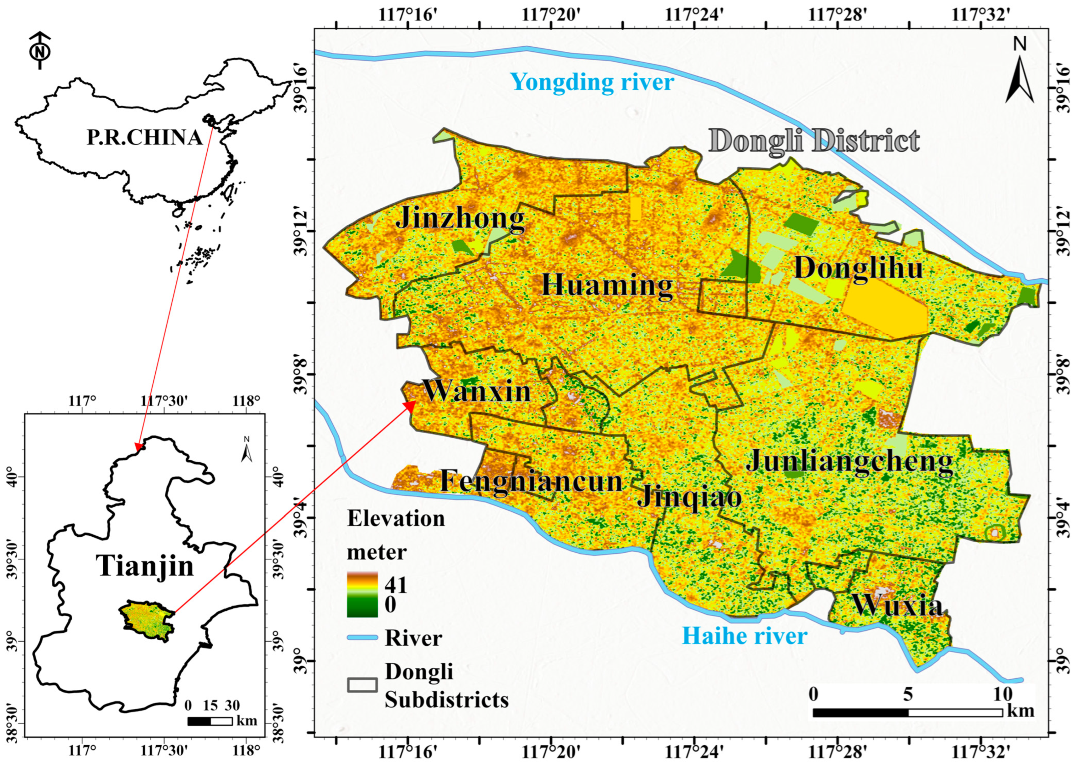
Tianjin is located on the coast of the Bohai Sea in northern China, with the Yanshan Mountains to the north [35,36]. Tianjin’s territorial boundary is approximately 1290 km, including 153 km of coastline and 1137 km of land boundary. The total area is 11,916.90 km2, with a sea area of over 3000 km2 [37]. It includes 16 districts, and the Dongli District is mainly discussed. It is located in the central-eastern part of Tianjin on the northern bank of the Haihe River (Figure 1). It spans 30 km east–west and 25 km north–south, covering a total area of 477.34 km2.

2.2. Geological Structure and Hydrostratigraphy

Tianjin’s geology is a coastal plain sequence of late Pliocene to Quaternary sediments over a structurally controlled bedrock, with a multi-layered aquifer–aquitard hydrostratigraphy that governs deformation behavior [38]. The aquifer system beneath Tianjin is commonly described as four principal aquifer groups (two shallow, two deeper confined aquifers as described in Table 1), with the deeper aquifers (often referred to as Aquifers III–IV as described in Table 1) hosting the long-term pumped groundwater system [34].
Groundwater in Tianjin comprises a multi-layered system whose long-term overextraction has produced deep drawdown cones and extensive compaction. Since the implementation of large surface water transfer and groundwater management (post-2014/2018), many deep aquifers have shown measurable rebound and reduced deformation [18,39,40]. Therefore, groundwater-level behavior shifted from continuous declines of 0.13–1.82 m (before remediation periods) to gradual rises of 0.45–1.87 m in the eastern plain after water-transfer interventions, as observed in multi-source monitoring datasets [18].
The upper two aquifers respond rapidly to recharge and seawater influence, while the lower two aquifers (deep confined units) experienced steady long-term declines over decades prior to remediation efforts [34]. Moreover, statistical and regression studies have identified drawdown in the second and third confined aquifers as the dominant drivers of strong and medium land deformation areas, informing critical water-level thresholds for management [41].

2.3. SAR Data Selection and InSAR Images Processing

This study primarily used Sentinel-1A satellite data, which are part of the European Space Agency’s (ESA) Copernicus program. A total of 149 Sentinel-1 C-band acquisitions acquired between June 2019 and June 2024 were used in this study. The data were collected in the ascending orbit direction along path 69, VV polarization. All SAR images were downloaded from the ESA Copernicus Open Access Hub. In addition, a 12.5 m resolution ALOS digital elevation model (DEM) was used for topographic phase removal during InSAR processing.
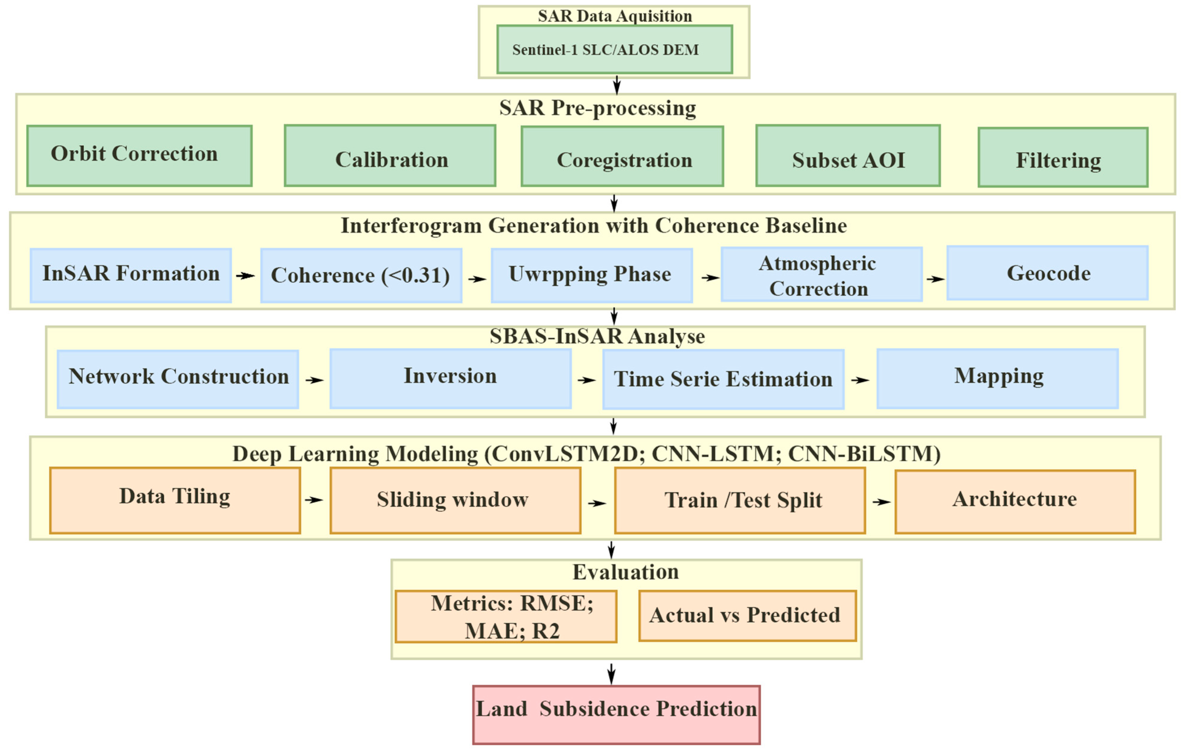
This study presents a useful approach for monitoring and predicting land deformation (Figure 2). It integrates an InSAR time-series analysis based on a coherence baseline for interferogram pair selection and advanced deep learning techniques for land deformation forecasting. The process begins with SAR data preprocessing and interferogram generation, followed by the derivation of time-series deformation maps using the SBAS-InSAR method. This deformation data served as the input to train and evaluate three distinct hybrid deep learning architectures (CNN–bidirectional long short-term memory (CNN-BiLSTM), CNN-LSTM, and 2D convolutional LSTM (ConvLSTM2D)) to identify the most effective model for accurate land deformation prediction.

2.3.1. Differential Interferometry

A temporal baseline threshold or spatial baseline threshold is set to filter the interferometric pairs, resulting in a small baseline interferometric pair set containing M pairs, where
N + 1 2 < M < N N + 1 2
Based on one reference image (the main image), all other images were co-registered, and interferometric processing was performed on M interferometric pairs. Subsequently, the flat-Earth phase was simulated and removed based on the baseline information, and the topographic phase was simulated and removed using the 12.5 m resolution ALOS DEM data, yielding M differential interferograms.
δ φ j x , γ = φ t B , x , r φ t A , x , r φ d i s p + φ t o p o + φ o r b + φ a t m + φ n o i s e
Equation (2) describes the composition of the interferometric phase in pixel (x, r) for interferogram j (generated from two images at t A and t B ), where x and r represent the azimuth and range coordinates, respectively. The phase φ d i s p arose from range variations along the line-of-sight (LOS) between the target and the radar. Furthermore, the phases φ t o p o , φ o r b , φ a t m , and φ n o i s e originated from residual topography, satellite orbit errors, atmospheric effects (particularly tropospheric delay), and other noise sources.

2.3.2. Coherence Baseline-Based Interferometric Pair Selection Method for Surface Deformation Monitoring

To overcome the disadvantages of conventional baseline selection methods, a technique that employs a coherence baseline instead of a temporal baseline was used for interferogram evaluation. This approach is based on the principle that temporal baselines are an indirect proxy for quality, whereas the average coherence provides a direct measure of the phase signal-to-noise ratio (SNR) [32]. Following the selection strategy proposed in the recent literature, we prioritized interferograms that maintained high phase stability over time, ensuring a more redundant and reliable network for inversion. This technique assesses the quality of interferometric images by referring to a quantitative measure of the interferometric pairs using an average coherence value. This value of average coherence, γ a v g , can be computed by using the formula expressed by Equation (3) [33].
γ a v g = i = 1 w j = 1 l γ ( i , j ) w l
where w is the image width, l is the image height (both in pixel units), and γ ( i , j ) is the coherence value at pixel i , j [33].

2.4. Hybrid Spatiotemporal Architectures for Deformation Forecasting

This study employed a deep learning approach based on ConvLSTM2D, hybrid CNN-LSTM, and hybrid CNN-BiLSTM networks to model and forecast the spatiotemporal patterns of land deformation. These three specific architectures were selected to evaluate different strategies for handling InSAR-derived time-series data. ConvLSTM2D integrates convolutions directly into the recurrent cells for unified spatiotemporal learning, whereas CNN-LSTM/BiLSTM hybrids utilize a modular approach to separate spatial feature extraction from temporal sequence modeling. This comparative framework allows for the identification of the optimal balance between spatial local feature capture and long-term temporal dependency tracking, which is theoretically essential for the nonlinear nature of land deformation. The processing was structured into five main phases: data preprocessing, model architecture design, training and validation, model comparison, and predictive forecasting.

2.4.1. ConvLSTM2D

The ConvLSTM2D layer is a recurrent layer that combines the convolutional and LSTM capabilities. It is used to capture spatiotemporal features, thereby improving the forecasting accuracy and computational efficiency of models [29,30]. Therefore, convolutional LSTM (ConvLSTM) and LSTM are essentially the same in terms of their working mechanisms [29].
The mathematical formulation of the ConvLSTM2D layer is as follows:
i t = σ X t W x i + H t 1 W h i + b i
f t = σ X t W x f + H t 1 W h f + b f
g t = σ X t W x g + H t 1 W h g + b g
O t = σ X t W x o + H t 1 W h o + b o
C t = f t C t 1 + i t g t
H t = O t tanh C t
where X t denotes the input at time t, H t represents the hidden state, C t indicates the cell state, W is the weight matrices, b is the bias vector, ∗ denotes the convolution operation, ⊙ represents element-wise multiplication, and σ denotes the sigmoid function. Equations (4) and (5) calculate the activation of the input gate i t and forget gate f t , respectively. The calculation of i t and f t involves the evaluation of X t , the previous hidden state H t 1 , and respective bias terms b i and b f using the convolution operation. It determines the specific information that needs to be updated within the cell state.
In this study, the initial layer used 64 filters and a (5, 5) kernel, followed by a second layer using 64 filters and a (3, 3) kernel. The final encoder layer uses 64 filters with a (1, 1) kernel. The decoder contains one Conv2D layer that transforms the spatiotemporal features of the encoder into the final prediction of the output. The layer uses one filter and a (3, 3) kernel with a sigmoid activation function to restrict the output values to the interval [0, 1].

2.4.2. Hybrid CNN-LSTM Model

A CNN encoder was first constructed to learn spatially relevant features from each image in the input sequence. The CNN subnetwork consists of three convolutional layers with rectified linear unit (ReLU) activation. The first layer uses 32 filters, and the second and third layers use 64 and 128 filters, respectively. Each convolutional layer was followed by a MaxPooling2D layer with a pool size of (2, 2).
The final output of the LSTM layer was passed through a dense decoder network to reconstruct the image. The decoder begins with a dense layer, the number of neurons of which is the total number of pixels in the target image (height × width × channels). A sigmoid function is applied as an activation function for this layer to generate output values in the range [0, 1]. The final step involved reshaping this one-dimensional output vector back into a two-dimensional image with the original target dimensions.

2.4.3. Hybrid CNN-BiLSTM

CNN-BiLSTM is a deep learning technique that integrates CNN and BiLSTM. This technique was primarily developed to handle sequential datasets with spatiotemporal information [23]. The main concept of this method revolves around the extraction of local spatial information using a CNN and the analysis of long-term dependencies of the temporal series using BiLSTM [42].
In this study, the Bi-LSTM architecture was the same as the hybrid CNN-LSTM architecture. The only difference is in place of the LSTM, we used the BiLSTM network.

2.4.4. Hybrid Spatiotemporal Architectures: Data Preprocessing, Sequence Generation, and Partitioning Strategy

A predictive framework was developed using 126 multi-temporal deformation maps, resampled to 124 × 124 pixels and normalized to [0, 1]. To suit the ConvLSTM2D, CNN-LSTM, and CNN-BiLSTM architectures, a sliding window (look-back of 10 steps) generated 116 supervised learning sequences. The dataset was partitioned into training (80%, n = 92) and validation (20%, n = 24) subsets using a fixed seed (n = 42) to ensure reproducibility of the results.

2.4.5. Performance Metrics

In this study, the model performance was assessed using several metrics, such as the mean squared error (MSE), root mean squared error (RMSE), mean absolute error (MAE), and coefficient of correlation (R2).
M A E = 1 m i = 1 m y i y ^ i
M S E = 1 m i = 1 m y i y ^ i 2
R M S E = M S E
R 2 = 1 i = 1 m y i y ^ i 2 y i y ¯ i 2
where m is the total number of data points, y i is the actual observed value, y ^ i is the predicted value, and y ¯ i is the mean of the actual observed value.
The overall methodology of this study is based on a combined framework that combines small baseline subset InSAR (SBAS-InSAR) with advanced deep learning architectures to monitor and predict land deformation with high precision. The workflow begins with the acquisition of Sentinel-1 SLC and ALOS DEM data, as illustrated in Figure 2, and continues with rigorous SAR preprocessing and the creation of interferograms that are limited by a threshold of 0.31 as the coherence baseline threshold, to ensure that the interferograms remain stable. The coherence threshold of 0.31 was determined by analyzing the coherence distribution of all interferogram pairs and testing different values to balance interferogram quality and network connectivity. Lower thresholds increase the number of interferograms but introduce more decorrelation, while higher thresholds improve quality and reduce decorrelation. Moreover, by using SBAS-InSAR analysis, such as network building and least-squares inversion, a high-resolution time-series deformation dataset was generated. The SBAS-InSAR processing in this study was carried out using the GAMMA remote sensing software package version 20240701. Furthermore, these spatial deformation maps were then fed through a sliding window and data tiling method to provide input into a series of hybrid neural networks, namely ConvLSTM2D, CNN-LSTM, and CNN-BiLSTM, which were trained to learn intricate spatiotemporal interactions. The models are finally tested against actual InSAR data with RMSE, MAE, and R2 techniques in order to provide a robust, predictive evaluation of land deformation patterns in the study region.

3. Results

3.1. InSAR Data Processing and Accuracy Evaluation

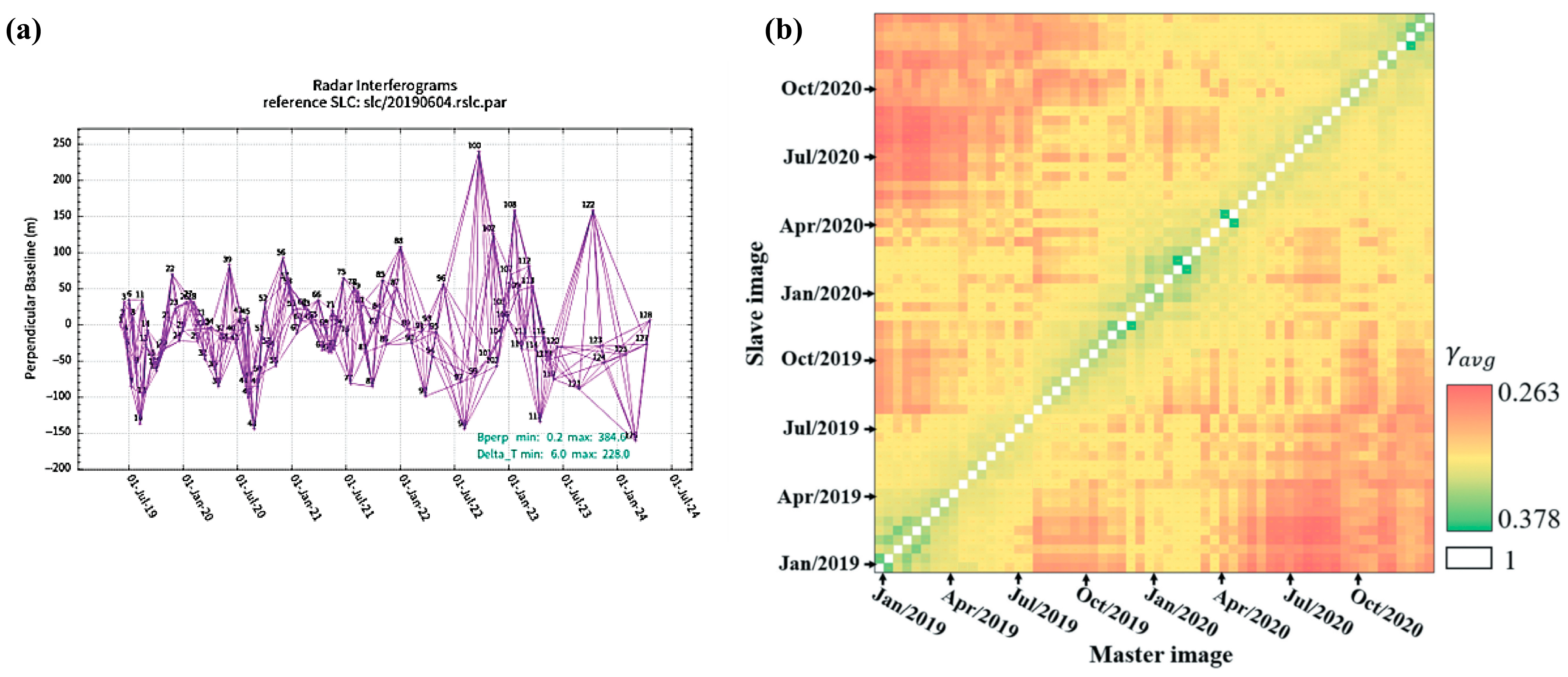
In this study, interferogram networks were first generated using a temporal baseline constraint to ensure network stability, followed by a coherence-based filtering step to retain high-quality interferograms for SBAS time-series analysis. The criteria for identifying the best SAR images for mapping with interferometric images were carefully considered. A maximum spatial baseline of 50 m and a temporal baseline of 60 days were applied to the Sentinel-1A images to meet the study requirements. This rigorous selection process ultimately yielded a final interferometric set of 625 pairs (Figure 3a). The number of usable interferograms is limited primarily because of the presence of strong temporal and spatial decorrelation, due to the presence of land cover that is mostly heterogeneous (urban/agricultural) and active groundwater-induced deformation, which results in poor phase stability for multi-temporal InSAR analysis.
Based on the coherence coefficient calculation formula (Equation (3)), a selected window size was applied to compute the coherence coefficient pixel by pixel for the filtered differential interferometric phase of the master and slave images, and a coherence map was generated (Figure 3b). Each small square represents an interferogram pair, and its color indicates the average coherence. The coherence of an image with itself is 1, corresponding to the diagonal line in the figure. However, because interferometry requires two images from different periods, the diagonal lines in the graph can be ignored. Therefore, based on the average coherence above 0.31, a total of 126 interferograms with good coherence were selected in this study.
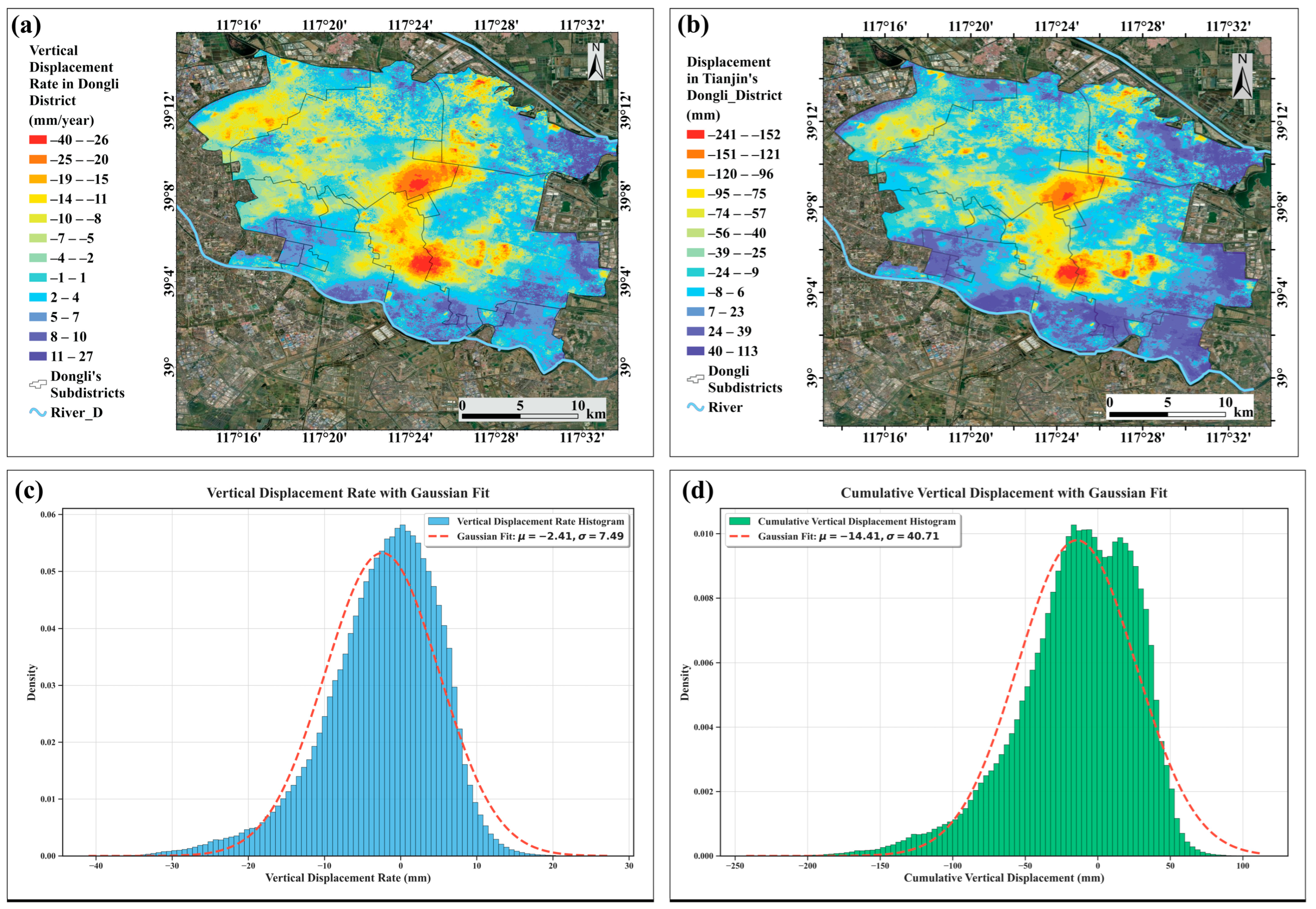
In total, 126 interferograms with a good coherence baseline were processed using the SBAS-InSAR technique. The InSAR measurements were initially obtained in the satellite line-of-sight (LOS) direction and subsequently converted to vertical deformation using the radar incidence angle through cosine projection, assuming negligible horizontal displacement relative to vertical subsidence. Thus, the final InSAR monitoring results for the Dongli District of Tianjin are shown in Figure 4. The Dongli District exhibited significant, widely dispersed, and large-magnitude deformation phenomena (Figure 4). Localized maximum deformation rates exceeded −40.00 mm/year, although the deformation rates typically ranged between 0 and −30.00 mm/year. Ground uplift was observed at certain locations. The spatial distribution of cumulative deformation in the Dongli District is consistent with that of the distribution of deformation rates during the monitoring period. The maximum cumulative deformation was −242.42 mm from 2019 to 2024, and the average maximum deformation rate was −40.98 mm/year (Figure 4a,b). The mean value ( μ = −2.41 mm/year) indicates that, on average, the district is experiencing a slight downward movement (Figure 4c). In addition, the mean cumulative deformation is μ = −14.41 mm (Figure 4d), suggesting that the “average” point in the district has sunk by nearly 1.44 cm from 2019 to 2024.

3.2. Accuracy Evaluation of InSAR Results

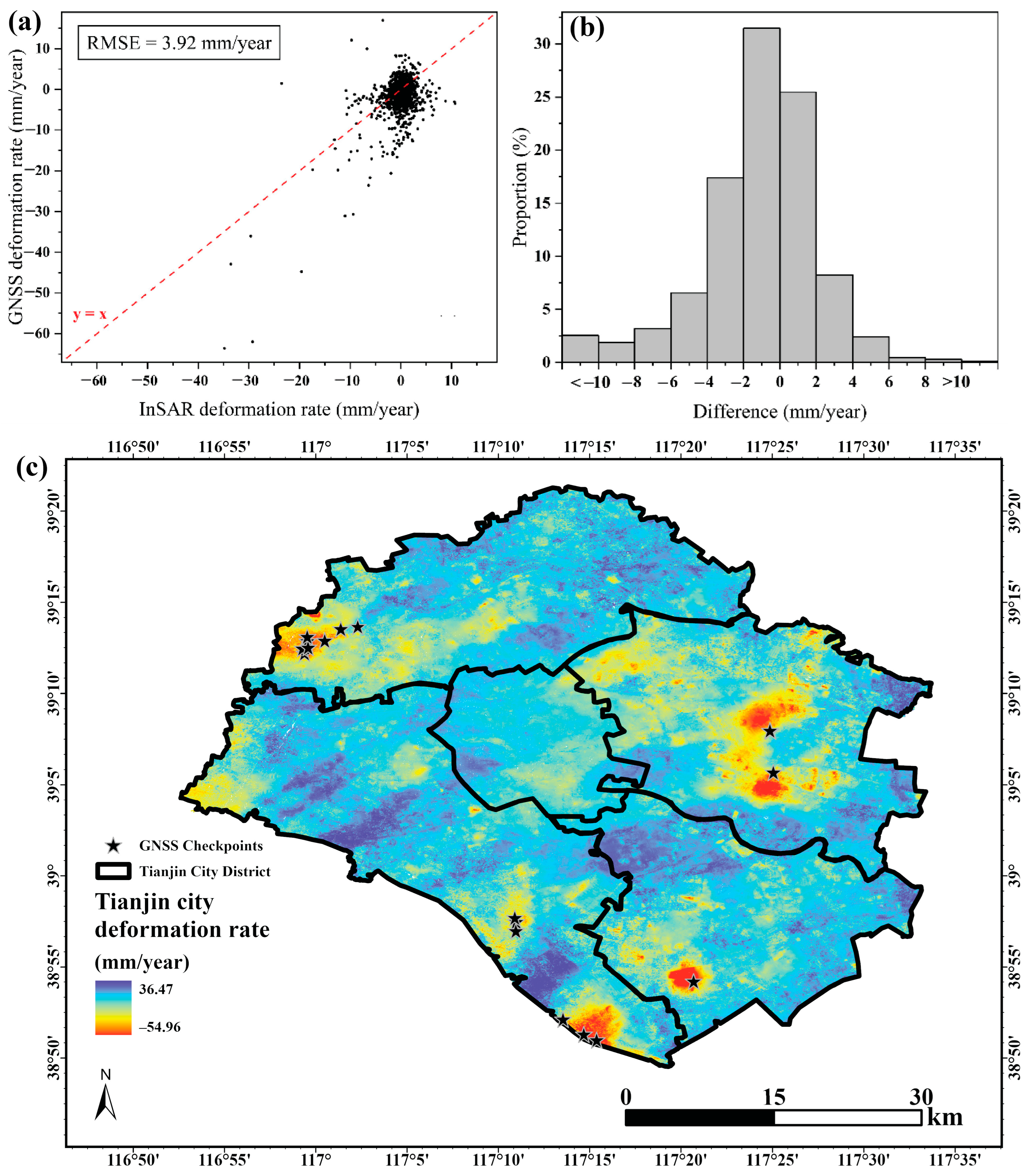
Beidou ground-based augmentation system (GBAS) network stations spread across the country’s land area were used as stations to verify the accuracy of the InSAR surface deformation monitoring results (Figure 5). There were 18 stations in the study (Figure 5c). These stations offer 24 h, continuous coordinate time series with a level of precision of millimeters.
To make a regular comparison, the daily GNSS coordinates were analyzed by linear regression to estimate the rate of deformation per year during the period of June 2019 to April 2024, which aligned with the InSAR observation period. A comparison of annual average deformation rates measured by the two datasets from June 2019 to April 2024 (Figure 5a) revealed that the errors generally followed a normal distribution with a root mean square error (RMSE) of 3.92 mm/year. This trend is also supported by the residual histogram in Figure 5b, which indicates that there is no systematic spatial or temporal bias in the InSAR measurements. As a result, the validated data show that it has adequate statistical reliability for application to engineering risk assessment.

3.3. Land Deformation Time Series in Dongli District from 2019 to 2024

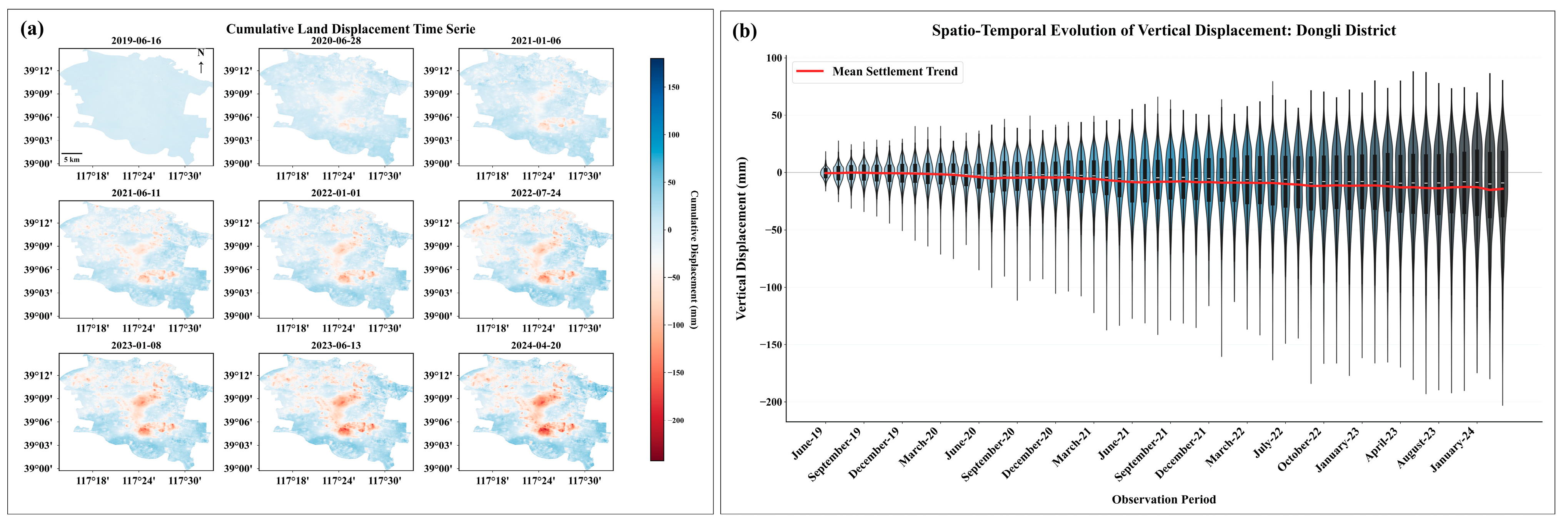
Ground deformation was inspected in the form of a time series in the Dongli District of Tianjin by contrasting the deformation values with the original image obtained on 10 June 2019 (Figure 6a,b). A complete analysis utilized 126 images to ensure high temporal density for model training. Figure 6a shows nine representative snapshots that visually capture the spatial progression of deformation from 2019 to 2024.
Figure 6b provides a statistical overview of this progression using 60 representative violin plots selected from the 126-image dataset. These plots demonstrate a widening distribution and a consistent shift in the median values toward negative deformation. The increase in the interquartile range over time indicates a diversification of deformation rates across the district, highlighting areas of accelerating deformation compared to more stable regions.

3.4. Spatial Distribution and Temporal Evolution of Land Deformation

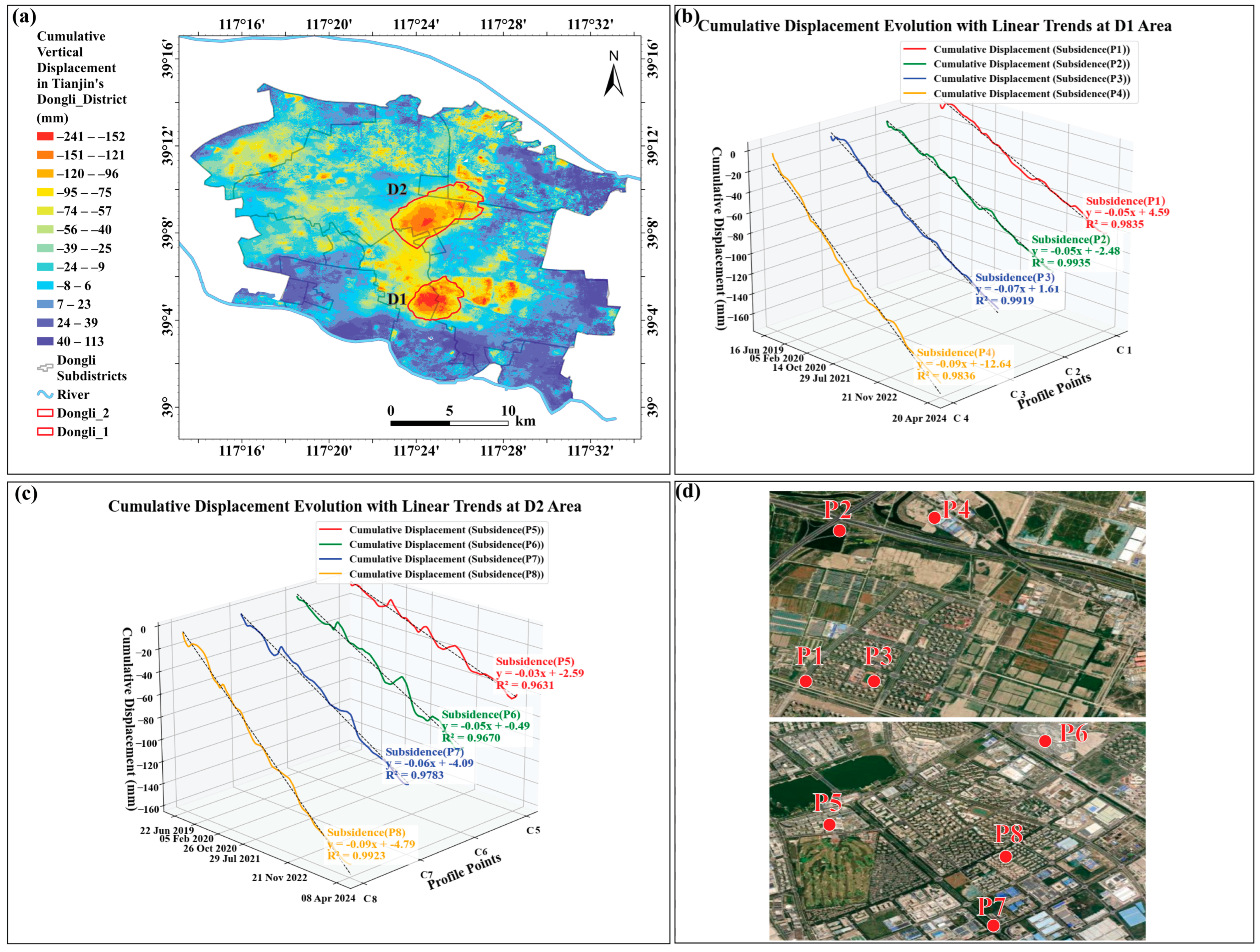
This study identified two zones in the Dongli District: Dongli 1 (D1) and Dongli 2 (D2). These zones were chosen to examine the typical areas of ground deformation, as shown in the InSAR land deformation map (Figure 7a). Detailed records were obtained for each investigation to assist in the subsequent analysis of the deformation results. This indicates diverse land deformation in the two zones, with D1 and D2 representing the highest levels of land deformation.
Figure 7 shows that the area marked as D2 experienced active deformation. This deformation was quite apparent and exceeded 200 mm, and the rates of deformation at this point fluctuated with a marked escalation before 2024. This information is of paramount importance for the surveillance of geological hazards and development planning for water resources and groundwater management.
The D1 plot provides unequivocal evidence of massive land deformation, with a cumulative sum of approximately 241 mm over five years. Sinking rates fluctuate, but net downward movement is unequivocally present. Land deformation at D1 and D2 was demonstrated by the data to be a fundamental problem, but of different magnitudes and in different modes that may be induced by variations in local geology, water management practices, or other environmental problems.
Both zones (D1 and D2) exhibited a steady, downward progression of cumulative vertical deformation with very high degrees of linearity. The high R2 values (all > 0.94) serve as mathematical validation that the “signal” is dominated by a strong linear trend rather than stochastic noise in these two zones. This suggests that the primary drivers, likely groundwater extraction or geological consolidation, are constant and have not been significantly offset by seasonal recharge during this interval. This signal stability was facilitated by implementing a refined average coherence baseline threshold (γ_arv > 0.31).

3.5. Spatiotemporal Deep Learning Model Performance Evaluation and Comparative Analysis

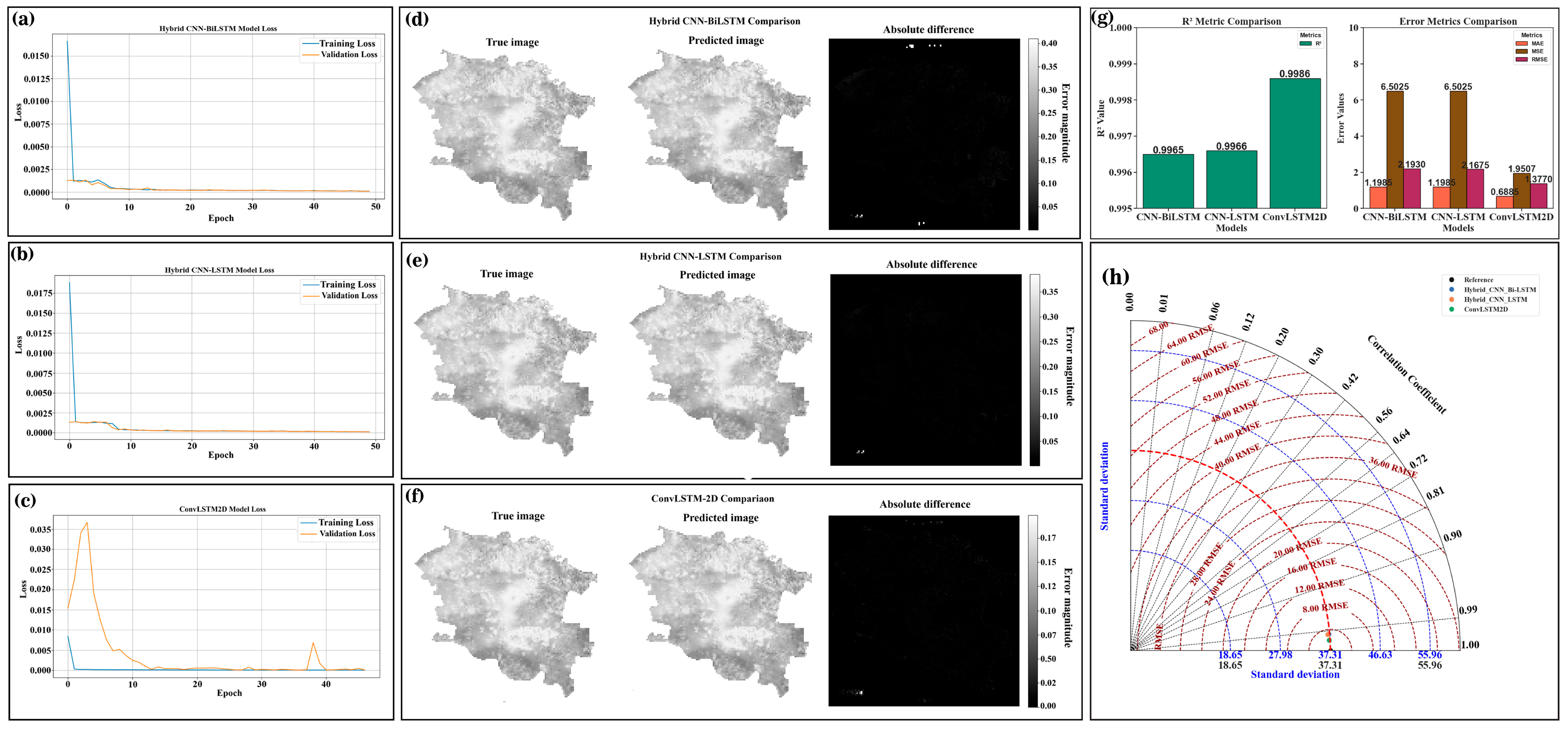
Figure 8 shows that the ConvLSTM2D model outperforms CNN-BiLSTM and CNN-LSTM in terms of training behavior, spatial reconstruction accuracy, and quantitative metrics (R2, MAE, RMSE, and Taylor diagram analysis) in all aspects, with the highest accuracy of convergence, lowest errors, and best agreement with the SBAS-InSAR deformation data.
The ConvLSTM2D model significantly outperformed both the hybrid CNN-LSTM and CNN-BiLSTM models across all key performance metrics, while it was computationally expensive in terms of training time (Table 2).
The ConvLSTM2D model represents the head and shoulders above its hybrid counterparts in terms of accuracy. Its mean absolute error (MAE) of 0.68 is substantially lower than the 1.19 and 1.19 of the hybrid CNN-LSTM and hybrid CNN-BiLSTM models, respectively. This indicates a significantly higher predictive accuracy. The same can be said for the mean squared error (MSE), with the ConvLSTM2D of 1.95 being one order of magnitude better than the 6.50 achieved by the other two models (Figure 8d–f).

3.6. Model Metrics Performance and Model Comparison

The ConvLSTM2D model had an R2 value of 0.99, which was practically a perfect fit for the data, explaining almost 99.90% of the variance. This makes the hybrid models’ performance redundant, with their respective R2 values of 0.99 and 0.99, which are much lower than the level of predictiveness.
The root mean squared error (RMSE) of the ConvLSTM2D model, at 1.37, was closest to half of the hybrid models (2.16 and 2.19). This large difference proves that the forecasts by the ConvLSTM2D model were always closer to the actual values. The standard deviation of the error also favors this, with a significantly narrower spread of prediction errors for the ConvLSTM2D model.
Although the hybrid versions significantly reduced training times (30–57 min), their execution time was at the cost of accuracy. The ConvLSTM2D architecture, even with its prohibitively long training period of more than 5 h, achieves a performance that is quite beyond the reach of the others. This suggests that, in high-precision operations, the computational expense of the ConvLSTM2D architecture is justified considering its output.
The ConvLSTM2D model was clearly the best performing among the three models (Figure 8). It exhibited the highest correlation, standard deviation that closely matched the reference data, and lowest RMSE. The diagram provides a compelling visual argument that, although all three models performed well, the ConvLSTM2D architecture was the most accurate and reliable for this prediction task.

3.7. Spatiotemporal Modeling and Prediction of Land Deformation

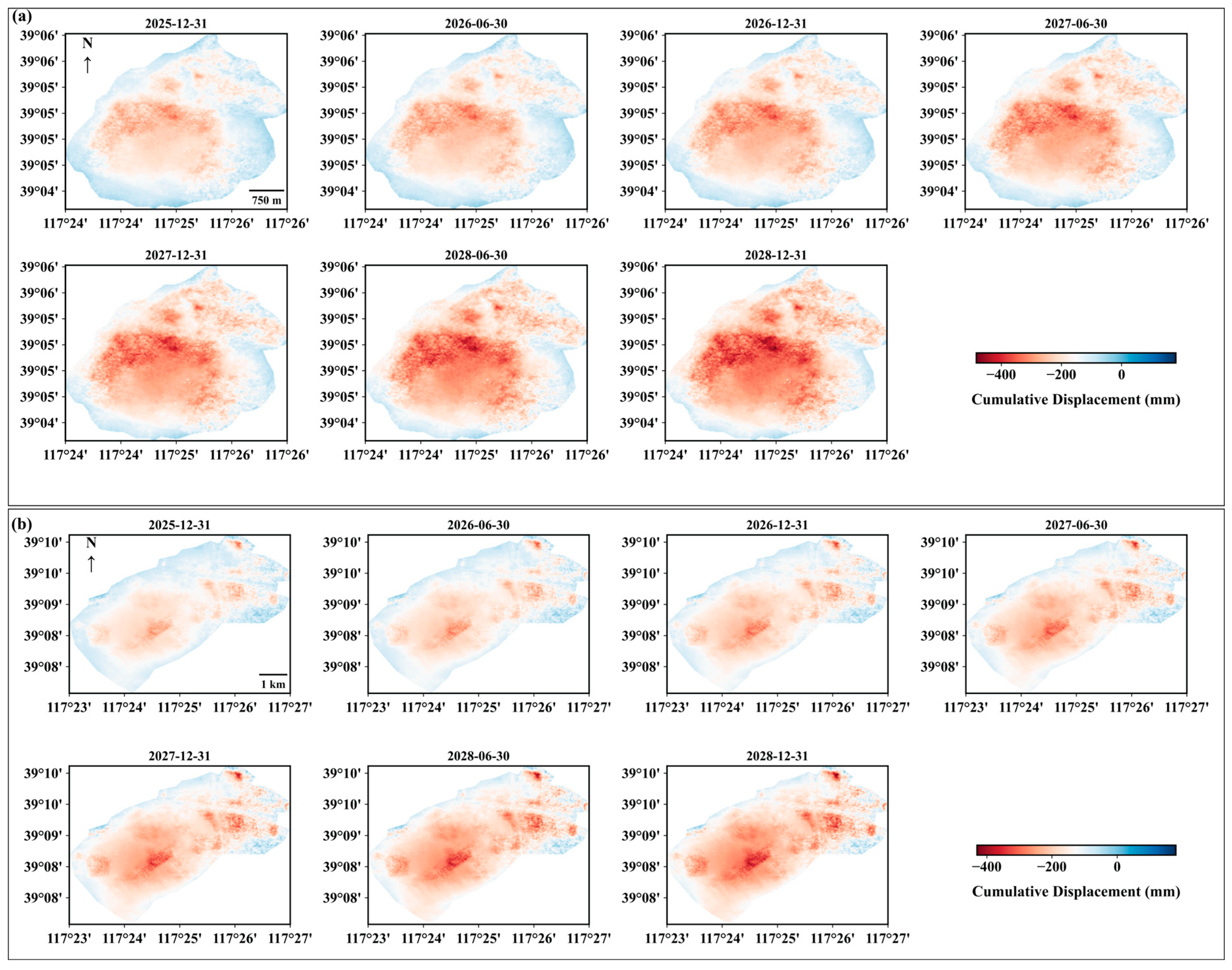
Land deformation in the Dongli District was predicted using ConvLSTM2D in the D1 and D2 zones from 2025 to 2028, as illustrated in Figure 9. The three-year prediction (2025–2028) was generated using a recursive feedback approach, where the predicted deformation map at step k served as a component of the input feature map for step k + 1. This allows the model to maintain the continuity of the deformation velocity field over the 36-month horizon. Projections of land deformation in the Dongli District, Tianjin, indicate significant differential movement by December 2028.
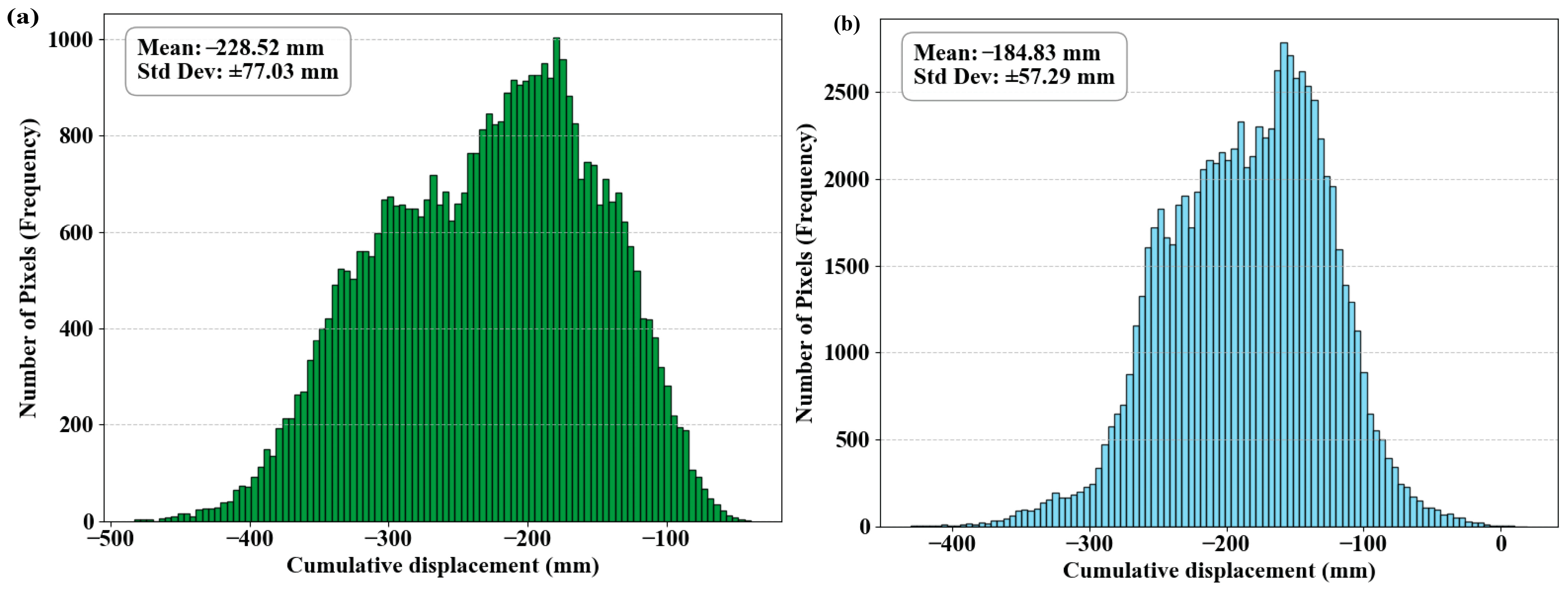
Figure 9. The land deformation prediction in the two chosen areas (D1 and D2) until 31 December 2028 was performed using ConvLSTM2D; (a) land deformation prediction at D1 area; (b) land deformation prediction at D2 area. Overall, there is a high degree of deformation in both regions based on the negative value of the mean. Nevertheless, their deformation properties can be distinguished. To begin with, the magnitude of deformation is greater in area D1, with the mean deformation being −228.52 mm, than in area D2, where it is −184.83 mm (Figure 10). Second, D1 (±77.03 mm) standard deviation is very large compared to that of D2 (±57.29 mm) from 2025 to 2028. It means that the deformation in area D1 is more spatially heterogeneous; i.e., there is a greater variety of deformation values in different pixels, but area D2 experiences a more homogenous process of deformation. Overall, it is expected that area D1 will be the worst-impacted and spatially complex zone of deformation at the end of 2028.
Remotesensing 18 02294 g009
Figure 10. The statistical distribution of predicted cumulative deformation from 2025 to 2028. (a) Histogram for area D1 (mean: −228.52 mm, std dev: ±77.03 mm); (b) histogram for area D2 (mean: −184.83 mm, std dev: ±57.29 mm).
Remotesensing 18 02294 g010
The analysis forecasts that the maximum land deformation will reach 450 mm with an annual deformation rate of 43.71 mm/year at monitoring point D1 and 426 mm with an annual deformation rate of 39.64 mm/year at monitoring point D2. These outcomes indicate a large spatial difference in vertical land movement, which needs to be investigated and treated.
These projections are mathematically grounded extensions of the robust linear trends established within the historical InSAR archive. These results underscore a critical requirement for integrated urban planning strategies that incorporate InSAR-based forecasting into long-term water resource management and geological hazard surveillance frameworks in the Dongli District.

4. Discussion

Groundwater extraction has been found to be the key factor causing land subsidence in previous studies conducted in Tianjin, especially in areas covered by thick compressible Quaternary sediments in districts [15,34]. Although groundwater regulation policies have been in place since the South-to-North Water Diversion Project [38] was launched, the findings of this study show that localized subsidence is still ongoing in several areas, which may be due to delayed hydrogeological recovery and compaction of low-permeability clay layers. In contrast, the observed uplift in the study area (Figure 4) may be associated with the hydrological impacts of this project.
Moreover, the good linearity of the deformation time series (R2 > 0.94) supports the hypothesis that the processes of subsidence in the investigated zones are mainly long-term persistent processes, rather than short-term episodic ones. In previous studies that used InSAR to investigate groundwater-induced subsidence, long-term deformation trends were nearly linear, caused by continuous compaction of the aquifer over multiple years [16,34,40]. The consistent deformation signal in D1 and D2 could suggest that the groundwater withdrawal rates were also fairly constant over the monitoring period, allowing for relatively continuous consolidation of compressible sediments.
Additionally, the performance of the ConvLSTM2D model is consistent with recent reports that spatiotemporal deep learning architectures can effectively predict spatiotemporal deformation, especially in geospatial applications [6,23]. This is the reason for the lower RMSE (1.37 mm) as well as prediction stability found in this study.
Furthermore, the proposed ConvLSTM2D framework has achieved high predictive accuracy compared to withheld SBAS-InSAR deformation observations, but the model is still data-driven and learns spatiotemporal patterns from historical deformation records only. Hence, the forecasting results are based on the assumption that the main deformation mechanisms and environment are relatively stable over the forecasting period. Variations in groundwater extraction rates, groundwater management policies, infrastructure developments, and external factors such as climatic conditions can lead to changes in future deformation behavior and uncertainties that cannot be captured explicitly in the present framework. Therefore, the forecasted deformation maps for 2025–2028 should be considered an indication of future deformation patterns from past observations, not as a physically predetermined set of projections. Groundwater-level observations, hydrogeological parameters, and land-use information, as well as other variables driving deformation, could be included in physics-informed deep learning hybrid models or in multi-source deep learning models in future studies, improving model generalization and physical interpretability.

5. Conclusions

This study successfully implemented a synergistic framework integrating high-resolution SBAS-InSAR monitoring with advanced deep learning architectures to characterize and forecast vertical deformation in the Dongli District, Tianjin. A critical methodological contribution was the application of a refined coherence baseline threshold (γ_arv > 0.31), which effectively mitigated temporal decorrelation and phase noise, thereby ensuring a high-fidelity geodetic dataset for subsequent predictive modeling.
The spatiotemporal analysis identified two prominent deformation hotspots, designated as D1 and D2, which exhibited persistent linear kinematic behavior. Between 2019 and 2024, these zones reached cumulative vertical deformations of 242 mm and 200 mm, respectively. The high degree of statistical linearity documented across these sites (R2 > 0.94) confirms that the deformation is governed by long-term anthropogenic or geological drivers, providing a robust empirical justification for the use of spatiotemporal deep learning in long-term projections.
Comparative model evaluation revealed that the ConvLSTM2D architecture significantly outperformed hybrid CNN-LSTM and CNN-BiLSTM counterparts, achieving a mean absolute error (MAE) of 0.68 and an R2 of 0.99. These metrics represent a substantial enhancement in predictive precision, despite the higher computational costs associated with the ConvLSTM2D training phase. Extended forecasts through December 2028 indicate that the deformation rate may escalate to maximum values of −43.71 mm/year at D1 and −39.64 mm/year at D2 from 2025 to 2028 in Dongli District, Tianjin.
Ultimately, these findings provide valuable information about the deformation patterns predicted by the model that may help decision-makers pinpoint areas that need more monitoring and mitigation efforts for urban planning in Dongli District, or for assessing the risk of land subsidence, and future studies that include additional deformation-driving factors, such as hydrogeological factors, will further help to interpret and predict the observed deformation trends physically. Moreover, the integration of InSAR-derived time series with ConvLSTM2D modeling offers a scalable and powerful framework for proactive geological hazard mitigation and sustainable water resource management in rapidly expanding urban environments.

Author Contributions

Conceptualization, J.M., H.L., Y.B. and W.L.; methodology, J.M., R.K.T., H.L. and W.L.; software, W.L.; validation, W.L.; formal analysis, W.L.; investigation, J.M., M.W., Y.Z., D.D., Y.G. and Y.B.; resources, J.M., Y.Z., D.D., H.L. and Y.G.; data curation, J.M., R.K.T., M.W., Y.Z., D.D., Y.G., Y.B. and W.L.; writing—original draft, R.K.T. and W.L.; writing—review & editing, J.M., H.L., Y.B. and W.L.; visualization, R.K.T.; supervision, J.M., H.L. and W.L.; project administration, J.M.; funding acquisition, J.M. All authors have read and agreed to the published version of the manuscript.

Funding

This research was supported by the Talent Cultivation Fund from the North China Center for the Geoscience Innovation of China Geological Survey (Grant no. 2024HBPJ-Q04); China Geological Survey Projects (Grant no. DD202606201403, DD20243452, DD20221727).

Data Availability Statement

The data presented in this study are available on request from the corresponding author.

Conflicts of Interest

The authors declare no conflicts of interest.

References

  1. Zhang, J.; Kou, P.; Tao, Y.; Jin, Z.; Huang, Y.; Cui, J.; Liang, W.; Liu, R. Urban ground subsidence monitoring and prediction using time-series InSAR and machine learning approaches: A case study of Tianjin, China. Environ. Earth Sci. 2024, 83, 473. [Google Scholar] [CrossRef]
  2. Zhou, H.; Dai, K.; Tang, X.; Xiang, J.; Li, R.; Wu, M.; Peng, Y.; Li, Z. Time-Series InSAR with Deep-Learning-Based Topography-Dependent Atmospheric Delay Correction for Potential Landslide Detection. Remote Sens. 2023, 15, 5287. [Google Scholar] [CrossRef]
  3. Ma, F.; Zhang, Q.; Sui, L. Prediction of old goaf residual subsidence integrating EDS-InSAR with EsLSTM in the Loess Plateau, China. Front. Earth Sci. 2025, 12, 1511785. [Google Scholar] [CrossRef]
  4. Zhang, Z.; Hu, C.; Wu, Z.; Zhang, Z.; Yang, S.; Yang, W. Monitoring and analysis of ground subsidence in Shanghai based on PS-InSAR and SBAS-InSAR technologies. Sci. Rep. 2023, 13, 8031. [Google Scholar] [CrossRef] [PubMed]
  5. Zheng, L.; Wang, Q.; Cao, C.; Shan, B.; Jin, T.; Zhu, K.; Li, Z. Development and Comparison of InSAR-Based Land Subsidence Prediction Models. Remote Sens. 2024, 16, 3345. [Google Scholar] [CrossRef]
  6. Wen, Y.; Wan, X.; Yuan, D.; Zhang, L.; Ge, D.; Zhang, L. C-LSTM for MT-InSAR Ground Deformation Prediction. In IGARSS 2024—2024 IEEE International Geoscience and Remote Sensing Symposium; IEEE: New York, NY, USA, 2024; pp. 11016–11019. [Google Scholar] [CrossRef]
  7. Zhang, X.; Cheng, Z.; Xu, B.; Gui, R.; Hu, J.; Yang, C.; Yang, Q.; Xiong, T. Coupling the Relationship between Land Subsidence and Groundwater Level, Ground Fissures in Xi’an City Using Multi-Orbit and Multi-Temporal InSAR. Remote Sens. 2023, 15, 3567. [Google Scholar] [CrossRef]
  8. Huang, L.; Zhu, P.; Zhang, T.; He, L.; Wu, W.; Ge, Z.; Ai, H. Investigation of land subsidence in Guangdong Province, China, using PS-InSAR technique. Adv. Space Res. 2025, 75, 3507–3520. [Google Scholar] [CrossRef]
  9. Zhao, D.; Yao, H.; Gu, X. Highway Deformation Monitoring by Multiple InSAR Technology. Sensors 2024, 24, 2988. [Google Scholar] [CrossRef] [PubMed]
  10. Weng, D.; Chen, W.; Lu, Y.; Ji, S.; Luo, H.; Cai, M. Global DGNSS service for mobile positioning through public corrections. Adv. Space Res. 2023, 72, 4402–4412. [Google Scholar] [CrossRef]
  11. Tao, Q.; Liu, R.; Li, X.; Gao, T.; Chen, Y.; Xiao, Y.; He, H.; Wei, Y. A method for monitoring three dimensional surface deformation in mining areas combining SBAS-InSAR, GNSS and probability integral method. Sci. Rep. 2025, 15, 2853. [Google Scholar] [CrossRef] [PubMed]
  12. Chen, S.; Ma, M.; Ma, Y.; Feng, X.; Xu, G.; Li, H.; He, Y. Three-dimensional deformation monitoring of San Francisco Bay based on GNSS-InSAR data. Adv. Space Res. 2025, 75, 451–464. [Google Scholar] [CrossRef]
  13. Usha, S.; Eatedal, A.; Nuha, A.; Wafa Sulaiman, A. Monitoring land subsidence using Sentinel-1A, persistent scatterer InSAR, and machine learning techniques. J. S. Am. Earth Sci. 2025, 155, 105433. [Google Scholar] [CrossRef]
  14. Xiao, Y.; Tao, Q.; Hu, L.; Liu, R.; Li, X. A deep learning-based combination method of spatio-temporal prediction for regional mining surface subsidence. Sci. Rep. 2024, 14, 19139. [Google Scholar] [CrossRef] [PubMed]
  15. Liu, P.; Li, Q.; Li, Z.; Hoey, T.; Liu, G.; Wang, C.; Hu, Z.; Zhou, Z.; Singleton, A. Anatomy of Subsidence in Tianjin from Time Series InSAR. Remote Sens. 2016, 8, 266. [Google Scholar] [CrossRef]
  16. Zhang, Y.; Wu, H.A.; Kang, Y.; Zhu, C. Ground Subsidence in the Beijing-Tianjin-Hebei Region from 1992 to 2014 Revealed by Multiple SAR Stacks. Remote Sens. 2016, 8, 675. [Google Scholar] [CrossRef]
  17. Yi, L.; Fang, Z.; He, X.; Chen, S.; Wei, W.; Qiang, Y. Land subsidence in Tianjin, China. Environ. Earth Sci. 2011, 62, 1151–1161. [Google Scholar] [CrossRef]
  18. Wang, K.; Wang, G.; Bao, Y.; Su, G.; Wang, Y.; Shen, Q.; Zhang, Y.; Wang, H. Preventing subsidence reoccurrence in Tianjin: New preconsolidation head and safe pumping buffer. Groundwater 2024, 62, 778–794. [Google Scholar] [CrossRef]
  19. Shang, J.; Wang, M.; Wang, X.; Yang, M.; Wu, Y.; Du, W. Three-dimensional surface deformation field monitoring and influencing factors analysis in mountainous areas based on SBAS-INSAR technology (Tianjin, China). Sci. Rep. 2025, 15, 25702. [Google Scholar] [CrossRef] [PubMed]
  20. Luo, Q.; Perissin, D.; Zhang, Y.; Jia, Y. L- and X-Band Multi-Temporal InSAR Analysis of Tianjin Subsidence. Remote Sens. 2014, 6, 7933–7951. [Google Scholar] [CrossRef]
  21. Liu, H.-H.; Zhang, Y.-Q.; Wang, R.; Gong, H.-L.; Gu, Z.-Q.; Kan, J.-L.; Luo, Y.; Jia, S.-M. Monitoring and analysis of land subsidence along the Beijing-Tianjin high-speed railway (Beijing section). Chin. J. Geophys. 2016, 59, 2424–2432. [Google Scholar] [CrossRef]
  22. Qiu, P.; Liu, F.; Zhang, J. Land Subsidence Prediction Model Based on the Long Short-Term Memory Neural Network Optimized Using the Sparrow Search Algorithm. Appl. Sci. 2023, 13, 11156. [Google Scholar] [CrossRef]
  23. Zhang, X.; Chen, Q.; Yang, M.; Zhao, Z.; Zheng, Y.; Dai, Q.; He, Y.; Cai, D.; Xu, T. Surface Deformation Monitoring and Prediction of Longtantian Open-Pit Mine Based on SBAS-InSAR and CNN-BiLSTM Techniques. IEEE J. Sel. Top. Appl. Earth Obs. Remote Sens. 2025, 18, 17706–17727. [Google Scholar] [CrossRef]
  24. Soni, R.; Alam, M.S.; Vishwakarma, G.K. Prediction of InSAR deformation time-series using improved LSTM deep learning model. Sci. Rep. 2025, 15, 5333. [Google Scholar] [CrossRef] [PubMed]
  25. Chen, T.; Ning, D.; Liu, Y. Land Subsidence Predictions Based on a Multi-Component Temporal Convolutional Gated Recurrent Unit Model in Kunming City. Appl. Sci. 2024, 14, 10021. [Google Scholar] [CrossRef]
  26. Azarm, Z.; Mehrabi, H.; Nadi, S. Enhanced Land Subsidence Interpolation through a Hybrid Deep Convolutional Neural Network and InSAR Time Series. Geosci. Model Dev. Discuss. 2024, 2024, 6903–6919. [Google Scholar] [CrossRef]
  27. Zhu, M.; Yu, X.; Tan, H.; Yuan, J.; Chen, K.; Xie, S.; Han, Y.; Long, W. High-precision monitoring and prediction of mining area surface subsidence using SBAS-InSAR and CNN-BiGRU-attention model. Sci. Rep. 2024, 14, 28968. [Google Scholar] [CrossRef] [PubMed]
  28. Kariminejad, N.; Mohammadifar, A.; Sepehr, A.; Garajeh, M.K.; Rezaei, M.; Desir, G.; Quesada-Román, A.; Gholami, H. Detection of land subsidence using hybrid and ensemble deep learning models. Appl. Geomat. 2024, 16, 593–610. [Google Scholar] [CrossRef]
  29. Feng, H.-Z.; Yu, H.-Y.; Wang, W.-Y.; Wang, W.-X.; Du, M.-Q. Recognition of mortar pumpability via computer vision and deep learning. J. Electron. Sci. Technol. 2023, 21, 100215. [Google Scholar] [CrossRef]
  30. Naz, F.; She, L.; Sinan, M.; Shao, J. Enhancing Radar Echo Extrapolation by ConvLSTM2D for Precipitation Nowcasting. Sensors 2024, 24, 459. [Google Scholar] [CrossRef] [PubMed]
  31. Xu, H.; Chen, F.; Zhou, W. A comparative case study of MTInSAR approaches for deformation monitoring of the cultural landscape of the Shanhaiguan section of the Great Wall. Herit. Sci. 2021, 9, 71. [Google Scholar] [CrossRef]
  32. Li, S.; Xu, W.; Li, Z. Review of the SBAS InSAR Time-series algorithms, applications, and challenges. Geod. Geodyn. 2022, 13, 114–126. [Google Scholar] [CrossRef]
  33. Wang, S.; Zhang, G.; Chen, Z.; Cui, H.; Zheng, Y.; Xu, Z.; Li, Q. Surface deformation extraction from small baseline subset synthetic aperture radar interferometry (SBAS-InSAR) using coherence-optimized baseline combinations. GISci. Remote Sens. 2022, 59, 295–309. [Google Scholar] [CrossRef]
  34. Su, G.; Xiong, C.; Zhang, G.; Wang, Y.; Shen, Q.; Chen, X.; An, H.; Qin, L. Coupled processes of groundwater dynamics and land subsidence in the context of active human intervention, a case in Tianjin, China. Sci. Total Environ. 2023, 903, 166803. [Google Scholar] [CrossRef] [PubMed]
  35. Huang, C.; Liu, K.; Ma, T.; Xue, H.; Wang, P.; Li, L. Analysis of the impact mechanisms and driving factors of urban spatial morphology on urban heat islands. Sci. Rep. 2025, 15, 18589. [Google Scholar] [CrossRef] [PubMed]
  36. He, Y.; Chen, T.; Zheng, Z.; Mi, F. Does urban green space justly improve public health and well-being? A case study of Tianjin, a megacity in China. J. Clean. Prod. 2022, 380, 134920. [Google Scholar] [CrossRef]
  37. Wang, G.; Duan, Z.; Yu, T.; Shen, Z.; Zhang, Y. Analysis of coastline changes under the impact of human activities during 1985–2020 in Tianjin, China. PLoS ONE 2023, 18, e0289969. [Google Scholar] [CrossRef] [PubMed]
  38. Liu, S.; Bai, M. Land subsidence along the Beijing-Tianjin high-speed railway before and after the South-to-North water diversion project with multi-source monitoring datasets. Front. Earth Sci. 2024, 12, 1372105. [Google Scholar] [CrossRef]
  39. Yu, H.; Gong, H.; Chen, B. Analysis of the Superposition Effect of Land Subsidence and Sea-Level Rise in the Tianjin Coastal Area and Its Emerging Risks. Remote Sens. 2023, 15, 3341. [Google Scholar] [CrossRef]
  40. Jiang, Z.; Zhu, J.; Guo, H.; Qiu, K.; Tang, M.; Yang, X.; Liu, J. South-to-North Water Diversion Halting Long-Lived Subsidence in Tianjin, North China Plain. Remote Sens. 2024, 16, 3213. [Google Scholar] [CrossRef]
  41. Qu, H.; Guo, Z. Study of Land Subsidence in Tianjin. In Geosciences and Human Survival, Environment, Natural Hazards, Global Change; CRC Press: Boca Raton, FL, USA, 2023; pp. 215–223. [Google Scholar]
  42. Alzubaidi, L.; Zhang, J.; Humaidi, A.J.; Al-Dujaili, A.; Duan, Y.; Al-Shamma, O.; Santamaría, J.; Fadhel, M.A.; Al-Amidie, M.; Farhan, L. Review of deep learning: Concepts, CNN architectures, challenges, applications, future directions. J. Big Data 2021, 8, 53. [Google Scholar] [CrossRef] [PubMed]
Figure 1. Overview map of the geographic location of the Dongli District, Tianjin.
Remotesensing 18 02294 g001
Figure 2. Flowchart of the integrated approach, which involves SBAS-InSAR time-series analysis with hybrid deep learning models for spatiotemporal prediction of land deformation. The green boxes represent the InSAR pre-processing stage, the blue boxes represent the InSAR processing stage, the orange boxes represent the hybrid deep learning stage, and the red boxes represent the final results.
Remotesensing 18 02294 g002
Figure 3. Spatial and temporal baseline distribution of Sentinel-1. (a) Interferometric pairs in the work area; (b) coherence map of interferogram selection.
Remotesensing 18 02294 g003
Figure 4. Vertical deformation rate and cumulative deformation in the Dongli District, Tianjin, from 2019 to 2024. (a) Deformation rate map; (b) cumulative deformation map (negative values indicate subsidence; positive values indicate uplift); (c) statistical overview of the vertical deformation rate in the Dongli District, Tianjin, as derived from the SBAS-InSAR analysis; (d) statistical overview of the cumulative deformation in the Dongli District, Tianjin.
Remotesensing 18 02294 g004
Figure 5. InSAR accuracy statistics. (a) Correlation between GNSS data and InSAR deformation results; (b) residuals distribution; (c) the 18 GNSS stations in Tianjin City.
Remotesensing 18 02294 g005
Figure 6. Vertical deformation time series in the Dongli District, Tianjin, from June 2019 to April 2024. (a) Vertical deformation time series of 9 different dates in the Dongli District, Tianjin, 2019–2024; (b) violin plots for land deformation in the Dongli District, Tianjin, from 2019 to 2024, with “Month abbreviation-YY” representing the month and year.
Remotesensing 18 02294 g006
Figure 7. Vertical land deformation evolution over time in the Dongli District, Tianjin, from June 2019 to April 2024. (a) Cumulative vertical deformation map highlighting two primary deformation zones (D1 and D2); (b) cumulative vertical deformation evolution at the D1 zone, where C1–C4 represent the temporal deformation curves for specific, representative points selected within deformation zone D1; (c) cumulative vertical deformation evolution at the D2 zone, with C5–C8 representing the temporal deformation curves for specific selected points in D2; (d) the detailed satellite imaging of each monitoring point at the D1 and D2 areas.
Remotesensing 18 02294 g007
Figure 8. Model evaluation and comparison. (a) Performance loss evaluation for hybrid CNN-BiLSTM model; (b) performance loss evaluation for hybrid CNN-LSTM model; (c) performance loss evaluation for ConvLSTM2D model; (d) true image, predicted and image difference in gray comparison for hybrid CNN-BiLSTM model; (e) true image, predicted and image difference in gray comparison for hybrid CNN-LSTM model; (f) true image, predicted, and image difference in gray comparison for ConvLSTM2D model; (g) models performance metrics comparison; (h) Taylor diagram for model comparison.
Remotesensing 18 02294 g008
Table 1. Principal aquifer groups beneath Tianjin.
Aquifer GroupApproximate Depth FocusPrimary Role and Behavior
Aquifer I (shallow)near surface to tens of metersResponds rapidly to precipitation and tidal/seawater influence and has limited long-term pumping [34].
Aquifer II (middle)tens to 100–200 mIt is commonly exploited for local use and contributes to intermediate responses [34].
Aquifer III (deep confined)100–300 m (monitoring and compressive layers around 94–182 m in some sites)It is a major historical exploitation layer and the principal source of inelastic compaction in many areas [34,39].
Aquifer IV (deepest confined)200–450 mDeep storage is subject to long-term drawdown and inelastic compaction in high-extraction zones [18].
Table 2. Performance metrics of different models.
ParametersConvLSTM2DHybrid CNN-LSTMHybrid CNN-BiLSTM
MAE0.681.191.19
MSE1.956.506.50
R20.990.990.99
RMSE1.372.162.19
Standard deviation of error1.352.162.16
Training time5.86 h0.51 h0.95 h
Disclaimer/Publisher’s Note: The statements, opinions and data contained in all publications are solely those of the individual author(s) and contributor(s) and not of MDPI and/or the editor(s). MDPI and/or the editor(s) disclaim responsibility for any injury to people or property resulting from any ideas, methods, instructions or products referred to in the content.