Article

Development of PXB-BVC Framework for Multivariate Flood-Risk Assessment Under Climate Change
1
School of Environmental Science and Engineering, Xiamen University of Technology, Xiamen 361024, China
2
Water Science and Environmental Research Centre, College of Chemistry and Environmental Engineering, Shenzhen University, Shenzhen 518060, China
3
Department of Civil and Environmental Engineering, Brunel University London, London UB8 3PH, UK
4
School of Climate Change and Adaptation, University of Prince Edward Island, Charlottetown, PE C1A 4P3, Canada
*
Author to whom correspondence should be addressed.
Remote Sens. 2026, 18(14), 2275; https://doi.org/10.3390/rs18142275
Submission received: 19 May 2026 / Revised: 13 June 2026 / Accepted: 29 June 2026 / Published: 8 July 2026

Highlights

What are the main findings?
  • The PXB-BVC model outperforms conventional hydrological models, with outstanding runoff simulation accuracy.
  • Climate change will drive a notable rise in watershed runoff, most prominently under the high-emission scenario; flood variable correlation strengthens and compound flood risks grow sharply.
  • Future extreme flood events will become far more frequent, and flood design values need to be greatly raised.
What are the implications of the main findings?
  • There is an urgent need to upgrade flood control facilities and build efficient early-warning systems to cope with intensified flood hazards.
  • Decision-makers can apply this model’s assessment results to formulate scientific flood prevention and climate adaptation strategies.
  • Future research should consider climate and land-use changes to further optimize hydrological prediction and risk evaluation.

Abstract

Flood risks are escalating under climate change, necessitating advanced methods to improve runoff prediction and multivariate flood-risk assessment. In this study, a physics–XGBoost-based Bayesian model averaging with bivariate copulas (PXB-BVC) framework was developed by integrating the Soil and Water Assessment Tool (SWAT), the Hydrologiska Byråns Vattenbalansavdelning (HBV) model, Extreme Gradient Boosting (XGBoost), Bayesian model averaging (BMA), and bivariate copulas. Spatially detailed underlying surface parameters including 30 m land-use data derived from the 2000 China land-use remote sensing monitoring data were pre-processed and reclassified using ArcGIS to support spatially explicit hydrological simulation. The framework was applied to the Xiangxi River Basin (XXRB), China, under four general circulation models and three shared socioeconomic pathways. PXB-BVC improved daily runoff simulation by combining process-based hydrological information with nonlinear machine learning correction, achieving Nash–Sutcliffe efficiency (NSE) values of 0.95 during calibration and 0.89 during validation. Future runoff generally increased from the near-term to the late-century period, with stronger changes under SSP585 and Sen slopes reaching up to 0.46 m3 s−1 yr−1, although the magnitude and significance of trends varied among GCMs. The dependence structures among flood peak, flood volume, and flood duration showed non-stationary behavior under future climate forcing, with Kendall’s tau for peak–volume pairs mostly ranging from 0.6 to 0.8. The revised bivariate return-period analysis further indicates that inferred flood-risk changes depend on the joint risk definition. Under SSP245 and ACCESS-ESM1–5, OR-type joint return periods show that representative near-future 50-year events may become more frequent in 2061–2100, whereas AND-type return periods show weaker and less uniform changes among flood-characteristic pairs. Conditional probability analysis also indicates enhanced compound risk under high-emission conditions: given an extreme peak flow, the probability of accompanying high flood volume increases from 0.23 to 0.56, while the probability of prolonged duration increases from 0.18 to 0.45. These results demonstrate that the PXB-BVC framework can support non-stationary multivariate flood-risk assessment and provide useful information for climate-resilient water-resource management and infrastructure planning.

1. Introduction

Floods are among the most devastating natural hazards, adversely affecting human safety, social development, and economic growth. This threat is being intensified by global climate change, as the Intergovernmental Panel on Climate Change (IPCC) projects the Earth to warm by more than 1.5 °C by 2040 [1]. Rising temperature can alter the spatio-temporal distribution of water resources by changing hydrological processes dominated by precipitation and evapotranspiration [2,3,4]. These changes introduce additional uncertainty into flood occurrence, magnitude, and frequency [5,6]. Recent CMIP6-based studies further indicate that high-emission scenarios may increase the likelihood and severity of extreme flooding, although the magnitude of change varies among regions and climate models [7,8,9]. Therefore, assessing future flood risk under climate change is crucial for water-resource management, flood-control planning, and infrastructure design.
Flood events are characterized by multiple attributes and their hazard level is jointly controlled by peak flow, flood volume, and flood duration [10]. Traditional univariate frequency analysis may be insufficient because it ignores the dependence among these flood characteristics. Multivariate joint-distribution methods, especially copula functions, have been widely used to characterize flood risk based on historical observations [11,12]. Recent studies have also developed multivariate frameworks for compound hydrological extremes and climate change-affected flood-frequency analysis [13,14]. However, many copula-based flood-risk studies still focus mainly on the statistical dependence structure of extracted flood events, whereas the upstream runoff-simulation chain used to generate future flood series is often simplified or treated separately. Under non-stationary climate conditions, future runoff generation and the dependence among flood variables may both change. It is therefore necessary to connect climate-driven runoff projection with multivariate flood-risk assessment in a unified framework.
Accurate runoff simulation and prediction are prerequisites for reliable flood-risk assessment, especially under the influence of climate change [15]. Hydrological models are important tools for runoff prediction [16,17] and can generally be categorized into process-based models (PBMs) and statistical-based models (SBMs). PBMs describe watershed hydrological processes using physically meaningful equations and parameters [18,19]. Among them, the Soil and Water Assessment Tool (SWAT) and the Hydrologiska Byråns Vattenbalansavdelning (HBV) model are widely used because of their physical interpretability and ability to simulate precipitation–runoff processes [20,21,22]. However, PBMs are affected by model-structure assumptions, parameter uncertainty, and input-data uncertainty. Their calibration can also be time-consuming because many parameters interact nonlinearly [23,24]. In contrast, SBMs can capture complex nonlinear relationships between environmental variables and runoff, but they are often criticized as “black-box” models with limited hydrological interpretability [25,26,27,28,29,30,31,32,33].
Coupling PBMs with machine learning models has therefore become an effective strategy for improving runoff simulation while retaining hydrological process information. Recent studies have shown that XGBoost, LSTM, Random Forest, and other machine learning models can improve streamflow or flood prediction by learning nonlinear rainfall–runoff relationships and correcting residual errors in process-based simulations [34,35,36,37,38,39]. These studies demonstrate the value of integrating physically based information with data-driven learning. However, most existing hybrid studies couple a single PBM with a machine learning algorithm. Because different PBMs represent runoff generation, storage, evapotranspiration, and routing processes differently, relying on only one PBM may not fully capture the hydrological behavior of a watershed. Multi-model fusion provides a potential way to reduce single-model uncertainty and use complementary hydrological information. Different PBMs may produce different runoff responses because of their distinct model structures and parameterizations [40]. Bayesian model averaging (BMA) is a useful method for combining multiple model outputs because it assigns weights according to model performance and posterior model probabilities, thereby reducing the risk of relying on a single model [41,42,43]. Recent studies have further shown that combining multiple hydrological models with machine learning methods can improve streamflow prediction and that Bayesian or copula-embedded averaging approaches can enhance hydrological ensemble prediction [37,44]. Nevertheless, calibration-only Bayesian weighting has not been sufficiently emphasized in many hybrid runoff-projection workflows. If validation-period observations are used during weight estimation, model performance may be overestimated because of information leakage. Therefore, a runoff-prediction framework that combines multiple PBMs, machine learning correction, and calibration-period BMA weighting is needed.
Based on the above review, three research gaps remain in previous multi-model fusion and copula-based flood-risk studies: (1) many existing hybrid hydrological models focus on the coupling of a single PBM and a single machine learning model, while the integration of multiple PBMs with machine learning correction remains limited; (2) although BMA has been widely applied to combine hydrological model outputs, few studies have used it to fuse multiple physics–machine learning coupled models, such as SWAT-XGBoost and HBV-XGBoost, and then linked the BMA-integrated runoff series with future bivariate copula-based compound flood-risk assessment; (3) previous studies have rarely connected future climate-driven runoff simulation with bivariate copula-based compound flood-risk assessment in a unified workflow. As a result, the link between improved runoff simulation and future multivariate flood-risk estimation remains insufficiently developed. To address these gaps, this study proposes a physics–XGBoost-based Bayesian model averaging with bivariate copulas framework, termed PXB-BVC, for runoff prediction and future flood-risk assessment in the Xiangxi River Basin. The framework first uses SWAT and HBV to represent complementary hydrological processes, then develops SWAT-XGBoost and HBV-XGBoost coupled models to correct nonlinear runoff-simulation errors, and finally combines the coupled-model outputs using calibration-period BMA weights. The resulting runoff series are used to extract flood peak, volume, and duration, and bivariate copula functions are applied to quantify joint return periods and conditional flood probabilities under CMIP6 climate scenarios. The novelty of this study lies in integrating these components into a coherent workflow for climate-driven runoff simulation and compound flood-risk assessment.
The central hypothesis is that a multi-physics, machine learning-assisted BMA framework can provide more reliable runoff simulations than single process-based or single machine learning benchmark models and that the resulting future runoff series can reveal non-stationary changes in multivariate flood risk under climate change. Accordingly, this study addresses three research questions: (1) Can the PXB-BVC framework improve daily runoff simulation relative to SWAT, HBV, MPM, and RF-based benchmark models? (2) How do future runoff and flood characteristics respond to different GCMs and SSP scenarios? (3) How do the dependence structures and joint return periods of flood peak, volume, and duration evolve under future climate forcing?
The remainder of this paper is organized as follows. Section 2 introduces the study area, datasets, PXB-BVC framework, model evaluation metrics, and multivariate flood-risk methods. Section 3 presents the runoff simulation, future runoff response, dependence structures, joint return periods, and conditional probability results. Section 4 discusses model performance, hydrological mechanisms, uncertainty, limitations, and transferability. Section 5 summarizes the main conclusions.

2. Materials and Methods

2.1. Case Study and Data

The upper reach of the XXRB is located in the western Hubei Province, China (110°17′–111°07′E, 31°03′–31°39′N). The XXRB is an important part of the Three Gorges Reservoir Region. As shown in Figure 1, the XXRB encompasses a catchment area of 3099 km2. The XXRB experiences a subtropical monsoon climate, with an average annual temperature of approximately 17.1 °C. Precipitation decreases from northwest to southeast, with an average annual rainfall between 900 and 1200 mm. The rainy season occurs mainly from June to September, exhibiting significant temporal and spatial variability. The river network in the XXRB is well-developed, making it susceptible to flood events triggered by localized heavy rainfall. Flooding can directly impact the basin’s economy, transportation, and social stability, creating an urgent need for precise flood-risk assessment and early-warning systems. This study forecasts future runoff in the XXRB and conducts flood-risk analysis to provide scientific support for flood prevention and disaster mitigation decisions by local governments.
The geographical spatial data include a Digital Elevation Model (DEM), land-use type, and soil type. The 30 m × 30 m resolution DEM data is provided by the Geographic Spatial Data Cloud website of the Computer Network Information Center, Chinese Academy of Sciences (http://www.gscloud.cn, accessed on 14 January 2025). The land-use dataset is derived from the 2000 China land-use remote sensing monitoring data of the Institute of Geographic Sciences and Natural Resources Research, Chinese Academy of Sciences, with a resolution of 30 m (http://www.resdc.cn, accessed on 23 January 2025), and the land-use data was reclassified using ArcGIS 10.8 software. The year-2000 land-use dataset was selected because it is close to the middle of the historical modeling period and provides complete high-resolution spatial coverage for the study area. Land use was kept static in both historical and future simulations; the implications of this assumption are discussed as a limitation in Section 4.3. Soil type data is sourced from the Harmonized World Soil Database (HWSD) with a spatial resolution of 1000 m × 1000 m. After identifying the soil types in the study area, SPAW 6.02 software was employed to calculate soil moisture characteristics for each soil type, such as hydraulic conductivity and available water content [45]. The daily obtained climate data from 1991 to 2008 are from the Xingshan meteorological Station in Hubei Province, China, including precipitation, temperature, evapotranspiration, and humidity. The hydrological model is calibrated and validated using daily runoff data from the Xingshan Hydrological Station for the period 1991 to 2008. Data pre-processing is shown in Table 1. The hydrological model developed in this study adopts a 12-year calibration period (1993–2004) and a 4-year validation period (2005–2008), as well as a 2-year warm-up period (1991–1992).
For the future period of 2025–2100, daily meteorological data were obtained from CMIP6. The Statistical Downscaling Model (SDSM) was employed to downscale precipitation and temperature data [46]. After calibrating the SDSM, validation was performed using observed meteorological data from 2005 to 2008, with rainfall data achieving a correlation of 0.53 and temperature data achieving a correlation of 0.91. This provides higher-precision input data for subsequent runoff forecasts. Detailed CMIP6 data information is available in Table 2.

2.2. PXB-BVC Framework

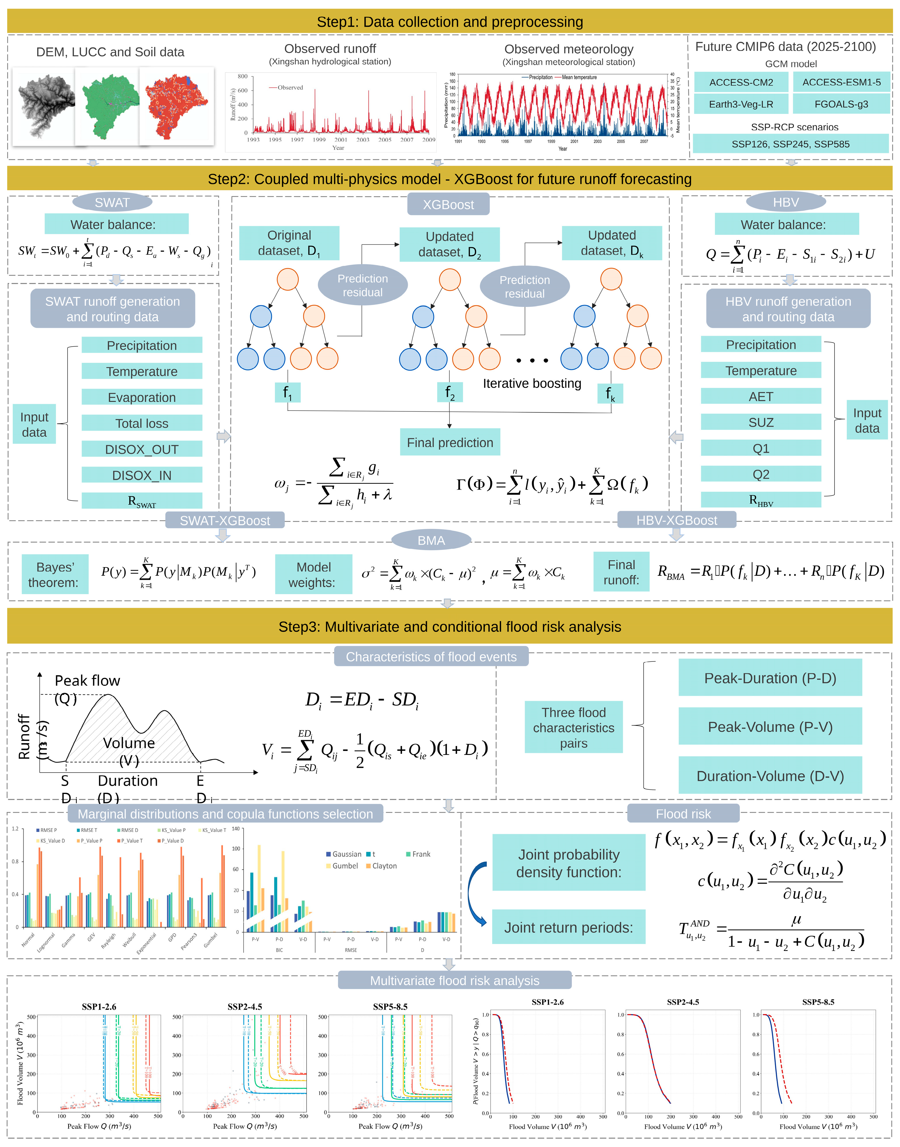
Figure 2 illustrates the framework of the PXB-BVC, which consists of four main steps: (i) data collection and pre-processing, (ii) development of a physics–XGBoost-based Bayesian model averaging with bivariate copulas (PXB-BVC) model, (iii) identifying the multiple variables of flood events based on flood peak, volume and duration, and (iv) multivariate and conditional flood-risk analysis. In fact, PXB-BVC leverages the synergistic advantages of PBMs and SBMs to enhance the robustness and physical interpretability of simulation outputs.

2.2.1. Multi-Physics Model

We used two PBMs, including SWAT and HBV models. The SWAT model is a process-driven, semi-distributed hydrological model widely used for simulating soil infiltration, runoff, and ecological interactions across large watersheds [17]. SWAT divides the watershed into sub-basins and further delineates Hydrological Response Units (HRUs) based on land use, soil type, and slope, enabling detailed simulation of spatially heterogeneous hydrological processes [37]. Model calibration and validation are performed using the SWAT-CUP tool with Sequential Uncertainty Fitting Version 2 (SUFI-2).
The HBV model is a simpler, semi-distributed, conceptual hydrological model designed for small watersheds and real-time forecasting. Its structure emphasizes low data requirements, making it effective for rapid response to precipitation events [16]. The XRBB is divided into five elevation zones and three vegetation zones based on DEM and land-use data. Parameter calibration and validation are performed using the HBV-light 2.0 software, employing the Monte Carlo method for parameter optimization. A total of 5000 iterations are conducted to identify the optimal parameter set. The descriptions, initial ranges, and optimal ranges of the selected parameters are presented in Tables S1 and S2 in the Supplementary Materials.

2.2.2. XGBoost

XGBoost, a machine learning algorithm based on gradient boosting, builds an ensemble of decision trees to iteratively optimize predictions. The advantages of the XGBoost model include high computational efficiency and the ability to capture complex nonlinear relationships. XGBoost minimizes a regularized objective function comprising a loss term and a regularization term, defined as:
Γ Φ = i = 1 n l y i , y ^ i + k = 1 K Ω f k
Ω f k = Υ T + 1 2 λ ω 2
where l y i , y ^ i represents the training loss function, which quantifies the deviation between the predicted y ^ i value and the actual observation y i . The term Ω f k serves as a regularization component designed to penalize the complexity of each individual tree fk, thereby mitigating the risk of overfitting. According to the definition of the regularization term in Equation (2), the model’s complexity is further refined by the total number of leaf nodes T and the L2 norm of the leaf weights ω , which are controlled by the complexity penalty coefficient γ and the regularization parameter λ respectively. During the optimization process, the algorithm iteratively constructs trees using gradient descent to minimize the overall loss. Furthermore, key hyperparameters including the learning rate, maximum tree depth, and the number of trees are typically optimized through a grid search to ensure the model achieves superior generalization performance.
In this study, XGBoost was used to develop two coupled models, namely SWAT-XGBoost and HBV-XGBoost. For each coupled model, XGBoost uses the outputs and selected process-related variables from the corresponding process-based hydrological model, together with meteorological variables, to predict observed daily runoff. For the SWAT-XGBoost model, the selected input variables include SWAT-simulated runoff (Qs), precipitation, temperature, evaporation, dissolved oxygen inflow and outflow, and nutrient-related outputs. The dissolved oxygen and nutrient-related variables are not interpreted as direct flood-driving factors; rather, they are SWAT-simulated internal transport-related outputs retained after correlation screening with observed runoff. For the HBV-XGBoost model, the selected input variables include HBV-simulated runoff and hydrological state or flux variables such as precipitation, actual evapotranspiration, potential evapotranspiration, upper-zone storage, and fast and slow runoff components. For both coupled models, the prediction target is the observed daily runoff at the Xingshan hydrological station.
The XGBoost hyperparameters were optimized using the Newton–Raphson-based optimizer (NRBO) with 5-fold cross-validation within the calibration period [47]. The cross-validation RMSE was used as the objective function, while R2, NSE, RMSE, and PBIAS were used for final model evaluation. The search ranges were 100–800 for the number of trees, 3–10 for maximum tree depth, and 0.0001–0.1 for the learning rate eta. The optimized parameters were num_trees = 112, max_depth = 3, and eta = 0.058708 for HBV-XGBoost and num_trees = 169, max_depth = 10, and eta = 0.071073 for SWAT-XGBoost. The regularization parameters gamma and lambda were not independently optimized and were kept at the default XGBoost settings.

2.2.3. BMA

BMA is used to synthesize the predictive outputs of multiple models through weights derived from posterior model probabilities. To avoid information leakage, the BMA weights in this study were estimated using only calibration-period model predictions and observed runoff. The obtained weights were then fixed and applied to the validation period and future projections [36,38]. This calibration-only weighting strategy was used consistently for MPM, PXB-BVC, and the RF-based benchmark ensemble. Detailed computational procedures are provided in the Supplementary Materials.

2.2.4. Model Performance Evaluation

The performance of SWAT, HBV, MPM and PXB-BVC is typically assessed based on the comparison of observed and simulated runoff. In this study, the statistical metrics of R-squared (R2), Nash–Sutcliffe efficiency (NSE), Root Mean Square Error (RMSE), Percent Bias (PBIAS) are employed to quantify the model’s performance [11,14].

2.3. Flood-Risk Analysis

2.3.1. Characteristics of Flood Events

Flood events during all study periods were extracted using the peak-over-threshold (POT) method, with a threshold value of the 90th runoff percentile. The typical characteristics of a flood event consist of flood peak flow (P), duration (D), and volume (V) [39]. In this study, the flood peak flow (Qi) is defined as the annual maximum value of daily runoff in the ith year; flood duration (Di) is defined as follows [7]:
D i = E D i S D i
where SDi and EDi are the start date and end date of a flood event for the ith year, respectively. The flood volume Vi can be calculated by the following [7]:
V i = V i t o t a l V i b a s e = j = S D i E D i Q i j 1 2 Q i s + Q i e 1 + D i
where Qij is the observed runoff in the jth day for the ith year; Qis and Qie are the observed runoffs on the start date and end date for the ith year, respectively. The term Di denotes the duration of the ith flood event. The three flood-characteristic pairs can be obtained through the above method (P-D, P-V, and D-V), and their dependence structure is modeled using a bivariate copula function.

2.3.2. Bivariate Copulas

The flood characteristics are not independent but exhibit complex interdependencies. For instance, a higher flood peak often corresponds to a longer flood duration or larger flood volume, and these relationships are typically nonlinear and asymmetric. Traditional methods relying on linear correlation measures are insufficient to accurately capture these dependencies. To address this, the copula method provides a powerful framework for modeling the dependence structure among flood characteristics. By separating the marginal distributions of individual variables from their joint dependency structure, copula functions enable flexible and precise modeling of multivariate relationships. This study employs bivariate copula functions to explore the dependence among the three flood characteristics, providing a robust basis for flood-risk assessment.
Copula functions join multivariate distribution functions with standard uniform margins, which represent the dependence structure of a vector of time-independent variables [40]. Based on Sklar’s theorem, a multivariate probability distribution F can be expressed as [5]
F x 1 , x 2 , , x n = C u 1 , u 2 , , u n
where u1 = FX1 (x1), u2 = FX2 (x2), …, un = FXn (xn) are continuous marginal distributions of random variables (x1, x2, …, xn). A copula function (C) can be written as [5]
C u 1 , u 2 , , u n = F F X 1 1 u 1 , F X 2 1 u 2 , , F X n 1 u n
For any given copula function, the conditional distribution for each xi can be achieved. Taking a bivariate copula as an example, the conditional distribution function of U1 with U2 = u2 and U2u2 can be achieved as follows:
C U 1 U 2 = u 2 u 1 = P U 1 u 1 U 2 = u 2 = C u 1 , u 2 u 2
C U 1 U 2 = u 2 u 1 = P U 1 u 1 U 2 u 2 = C u 1 , u 2 u 2
The probability density function (PDF) of a copula can be expressed as
c u 1 , u 2 = 2 C u 1 , u 2 u 1 u 2
Various copula families that represent different dependence structures have been developed, including elliptical, archimedean and extreme-value families [5]. In this study, 5 copula functions (i.e., Gaussian, Student t, Clayton, Frank and Gumbel copula) are used for screening out the appropriate copula functions for modeling the dependence structure of multiple flood characteristics [5,41,42]. The RMSE, Bayesian information criterion (BIC) and Squared Euclidean Distance (SED) are used for goodness-of-fit tests of copula functions [11,14].

2.3.3. Multivariate Hydrological Risk Analysis

The return period of a flood event is a basic criterion for design of hydrological infrastructure and provides a simple means of flood-risk analysis [43]. In multivariate flood-risk analysis, the joint return periods (i.e., “AND”) can be calculated as [44]:
T u 1 , u 2 A N D = μ 1 u 1 u 2 + C u 1 , u 2
T u 1 , u 2 O R = μ 1 C ( u 1 , u 2 )
The joint return periods for the AND and OR scenarios are defined by Equation (10) and Equation (11), respectively, where μ is the average inter-arrival time of events, u1 and u2 are the marginal probabilities, and C(u1, u2) denotes the copula function. The denominator represents the joint exceedance probability of both variables.

3. Results

3.1. Runoff Simulation Performance of the Coupled Models

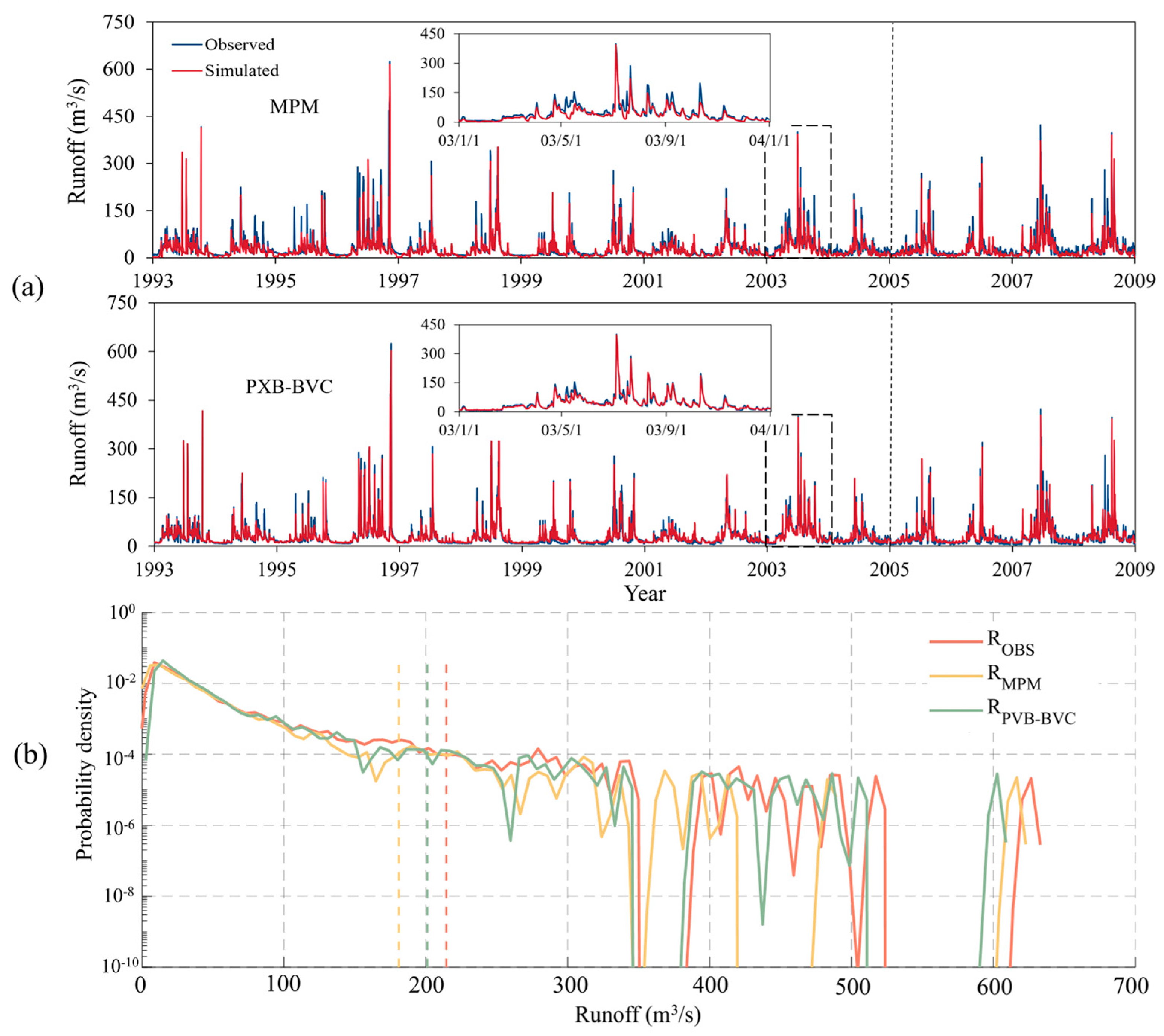
SWAT and HBV were combined into the multi-physics model (MPM) with weights of 0.613 and 0.387, respectively. SWAT-XGBoost and HBV-XGBoost were further combined into the PXB-BVC model with weights of 0.710 and 0.290, respectively. Figure 3a and Table 3 compare the daily runoff simulation performance of MPM and PXB-BVC during the calibration and validation periods. During calibration, MPM achieved R2 = 0.82, NSE = 0.79, PBIAS = −15.67%, and RMSE = 18.73 m3/s, whereas PXB-BVC achieved R2 = 0.95, NSE = 0.95, PBIAS = 0.91%, and RMSE = 9.43 m3/s. During validation, MPM achieved R2 = 0.78, NSE = 0.76, PBIAS = −16.58%, and RMSE = 15.37 m3/s, whereas PXB-BVC achieved R2 = 0.89, NSE = 0.89, PBIAS = 1.79%, and RMSE = 11.03 m3/s.
The near-zero PBIAS values of PXB-BVC indicate that the proposed framework substantially reduced the systematic underestimation observed in the process-based models. In the calibration period, SWAT, HBV, and MPM showed negative PBIAS values of −9.73%, −12.35%, and −15.67%, respectively, whereas PXB-BVC reduced the PBIAS to 0.91%. In the validation period, the corresponding PBIAS values of SWAT, HBV, and MPM were −9.45%, −16.30%, and −16.58%, while PXB-BVC achieved a much smaller PBIAS of 1.79%. Relative to MPM, the absolute PBIAS was reduced by 94.2% during calibration and 89.2% during validation.
To further examine the source of this bias reduction, the intermediate coupled-model outputs were compared. SWAT-XGBoost achieved PBIAS values of 1.02% during calibration and 2.81% during validation, while HBV-XGBoost achieved 0.97% during calibration and −2.31% during validation. These results indicate that XGBoost correction is the main step that reduces the systematic negative bias of the process-based models. The BMA step further balances the remaining branch-specific biases: during validation, SWAT-XGBoost shows a small positive bias, whereas HBV-XGBoost shows a small negative bias. Their BMA-weighted combination therefore produces a final PXB-BVC prediction with near-zero bias.
Figure 3b further shows that PXB-BVC reproduces high-flow events more closely than MPM, especially for runoff peaks above the 95th percentile. These results indicate that the coupled XGBoost-BMA framework improves both overall daily runoff simulation and peak-flow representation, providing a more reliable runoff series for subsequent future flood-risk analysis.

3.2. Future Runoff and Flood-Characteristic Responses Under Climate Change

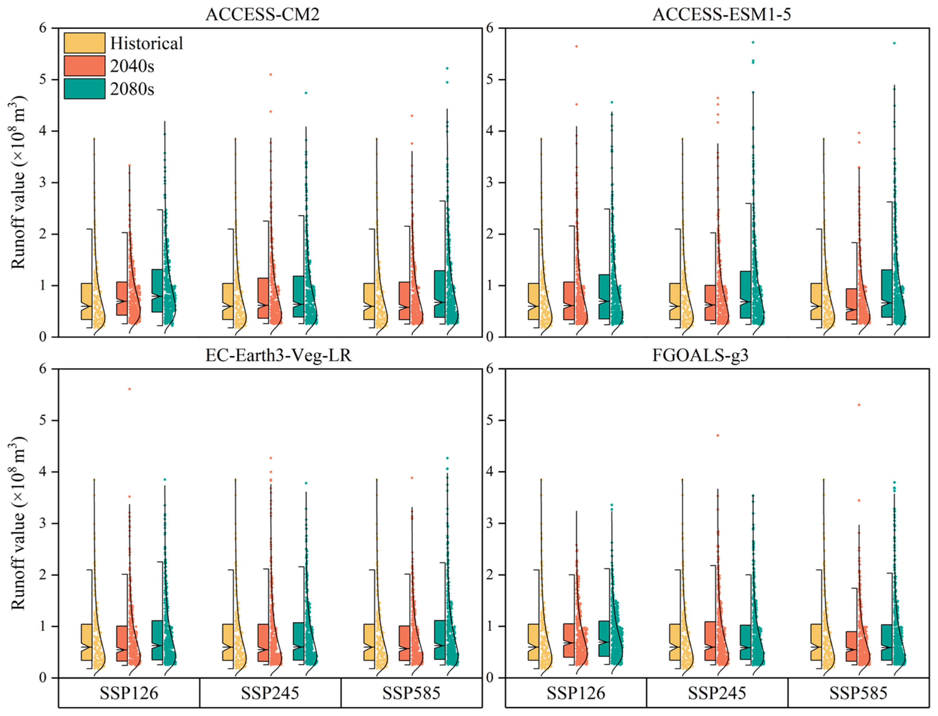
As shown in Figure 4 and Table 4, projected runoff differs among GCMs and SSP scenarios, reflecting differences in climate forcing and inter-model spread. Overall, runoff tends to increase from the near-term period to the long-term period, with stronger increases generally occurring under SSP585. For example, under SSP585, M1 shows a significant increasing trend, with a Sen slope of 0.43 m3 s−1 yr−1 and a Z-value of 3.00. In contrast, runoff changes under SSP126 are generally smaller, indicating a weaker climate change signal under the low-emission pathway.
Weak and statistically insignificant Sen slope values, including slight negative slopes in some GCM–scenario combinations, should not be interpreted as robust decreasing runoff trends. Instead, they indicate that the projected change signal is weak relative to interannual variability. Differences in Sen slope among GCMs under the same SSP mainly reflect uncertainty in climate-model projections, which is further propagated through downscaling and runoff simulation.
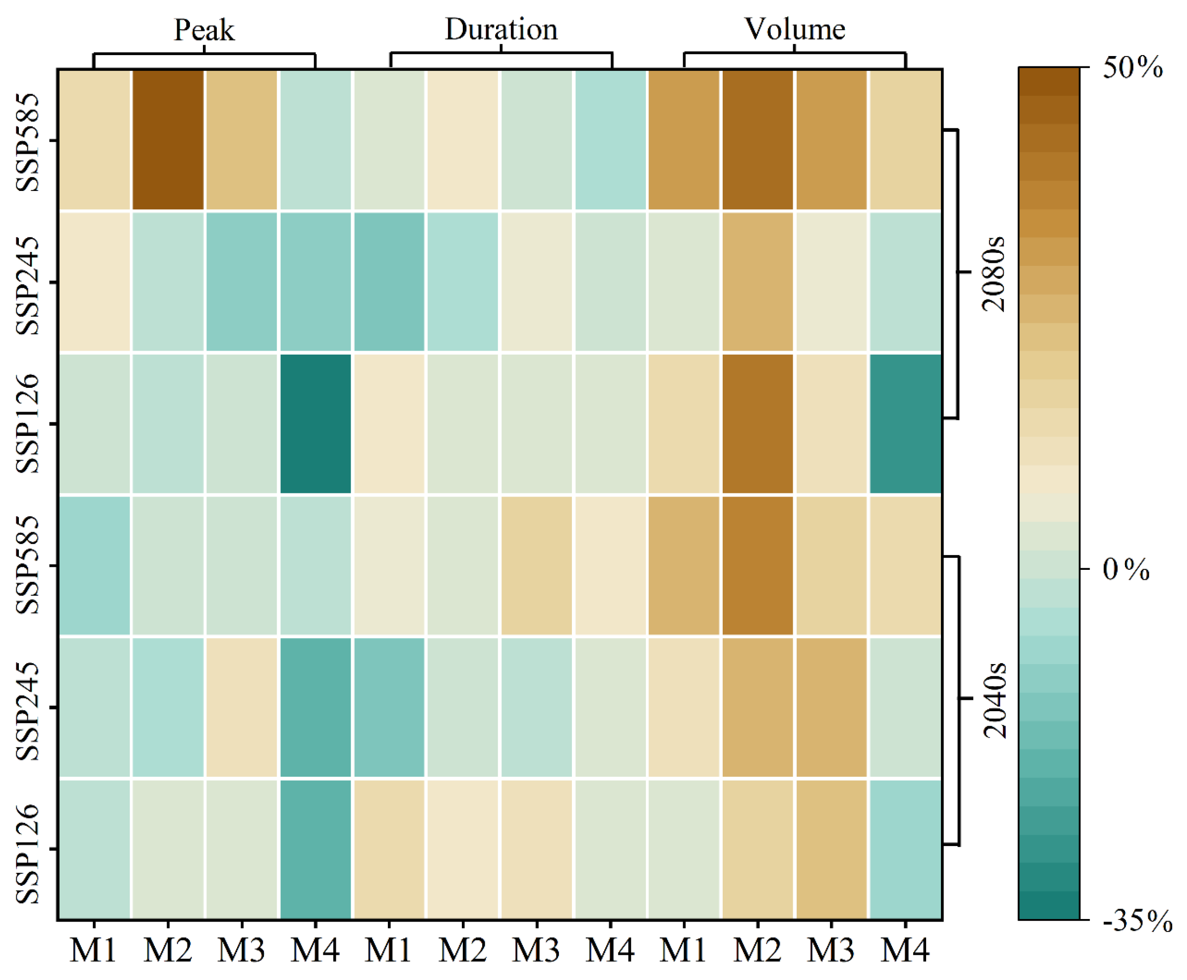
Figure 5 shows the median changes in flood peak, flood volume, and flood duration relative to the historical reference period (1993–2008). The most pronounced changes occur under SSP585 in the long-term period, especially for flood peak and flood volume. These results indicate that future climate forcing may increase not only mean runoff but also the magnitude of flood-related characteristics, thereby providing the basis for multivariate flood-risk assessment.
Overall, this study confirms that climate change has significantly influenced the trend of runoff changes in the basin. The continuous increase in runoff elevates the risk of flood events, while the increased frequency of extreme precipitation under SSP585 scenarios leads to higher hydrological uncertainty. These multidimensional characteristics of flood events necessitate the use of advanced techniques for joint risk assessment and underscore the growing challenges to environmental safety and water-resource management in the basin.

3.3. Multivariate Flood-Risk Changes Based on Bivariate Copulas

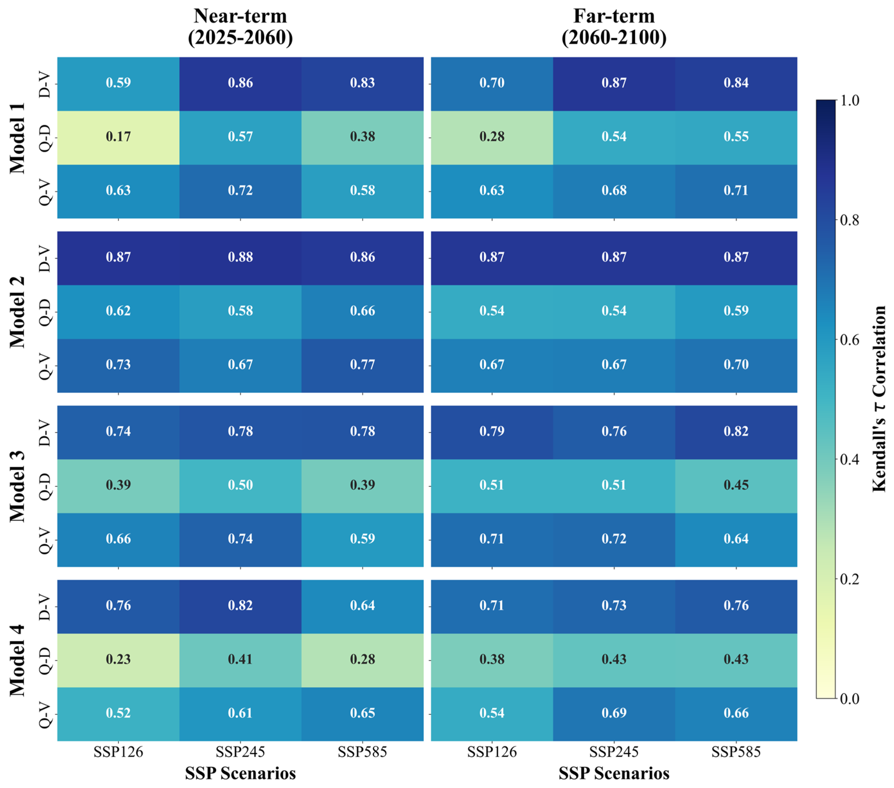
The dependence structures among flood peak (Q), volume (V), and duration (D) provide the statistical basis for multivariate flood-frequency analysis. Table 5 presents the selected copula functions, and Figure 6 shows Kendall’s rank correlation coefficients for flood-characteristic pairs under different GCMs, time periods, and SSP scenarios. Significant positive correlations were observed for most variable pairs, supporting the use of bivariate copulas to characterize joint flood-risk behavior. The strongest dependence generally occurs between Q and V, with Kendall’s tau mostly ranging from 0.6 to 0.8.
The dependence structures also show non-stationary features under future climate forcing. Although all variable pairs generally maintain positive dependence, the strength of dependence varies among SSP scenarios and GCMs. Under SSP585, the long-term dependence between flood magnitude and duration tends to strengthen relative to lower-emission scenarios, suggesting that future floods may be more likely to combine high peak flow, large volume, and longer duration.
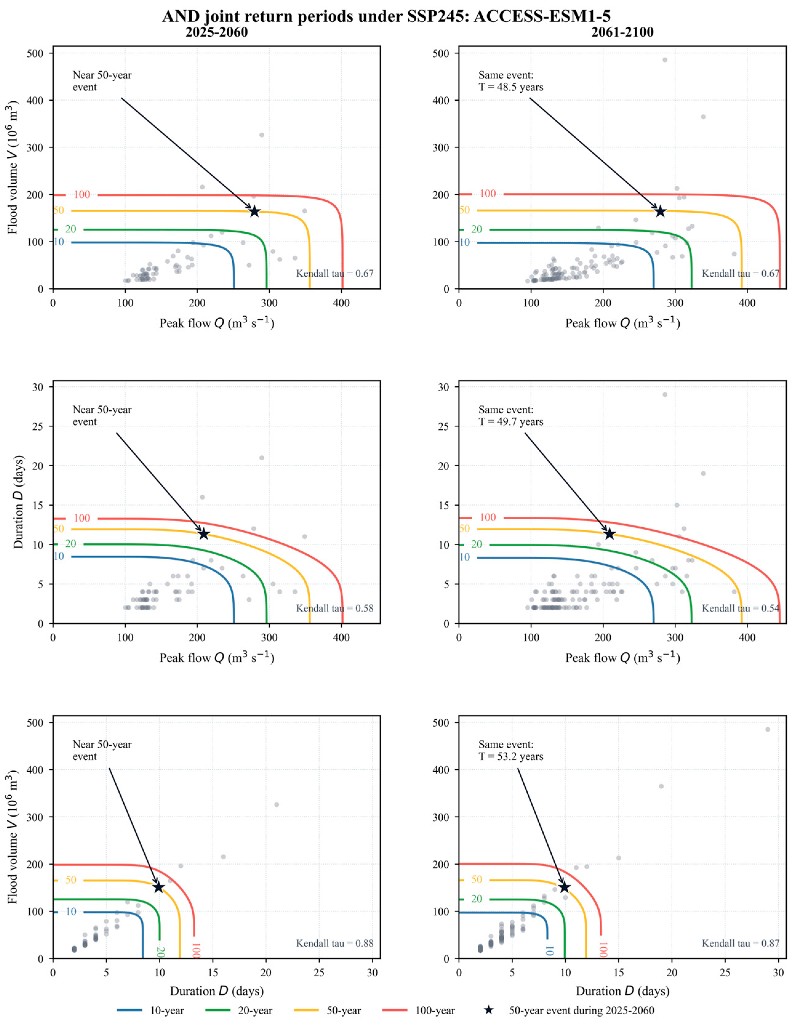
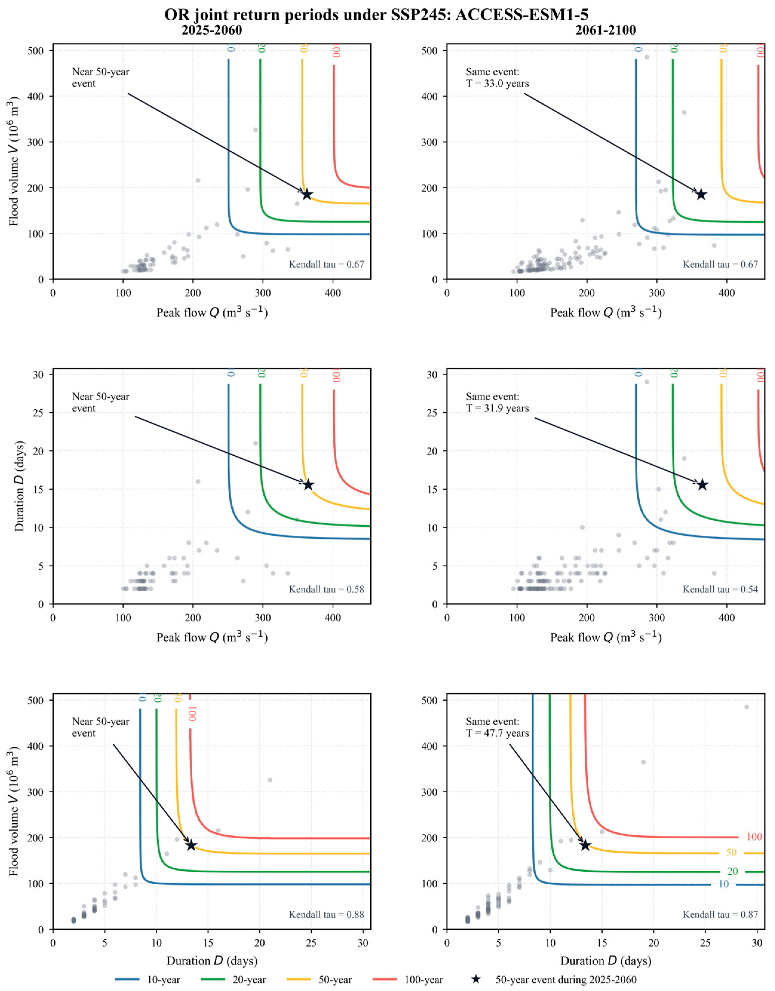
Figure 7 and Figure 8 were revised to improve the interpretability of the bivariate flood-risk results. Instead of presenting all SSPs in a single dense layout, the revised figures focus on SSP245 and compare the near-future period (2025–2060) with the late-century period (2061–2100). ACCESS-ESM1–5 was selected as the representative GCM because it provides a clear comparison between the two periods without producing excessively extrapolated return-period values. The star in each panel denotes a representative near-future 50-year event, and the corresponding late-century return period of the same event is annotated in the right column.
Under the AND joint return-period definition (Figure 7), the changes are relatively weak and depend on the selected flood-characteristic pair. For the peak flow–flood volume pair, a near-future 50-year event corresponds to a late-century return period of approximately 48.5 years. For the peak flow–duration pair, the same near-future 50-year event corresponds to approximately 49.7 years in 2061–2100. These two pairs therefore show a slight increase in event frequency. In contrast, the duration–flood volume pair changes from approximately 50.0 years to 53.2 years, indicating a slight decrease in frequency. Thus, the AND-type results suggest that simultaneous-exceedance risk does not change uniformly across all flood-characteristic combinations.
The OR joint return-period results show a more evident shift toward more frequent exceedance events (Figure 8). A near-future 50-year event becomes approximately a 33.0-year event for the peak flow–flood volume pair, a 31.9-year event for the peak flow–duration pair, and a 47.7-year event for the duration–flood volume pair in 2061–2100. This indicates that, when the exceedance of either flood characteristic is considered, late-century flood events under SSP245 may occur more frequently. The contrast between Figure 7 and Figure 8 demonstrates that inferred flood-risk changes depend strongly on the joint risk definition: OR-type return periods are more sensitive to changes in individual flood characteristics, whereas AND-type return periods emphasize simultaneous exceedance and therefore provide a more conservative estimate of compound flood risk.
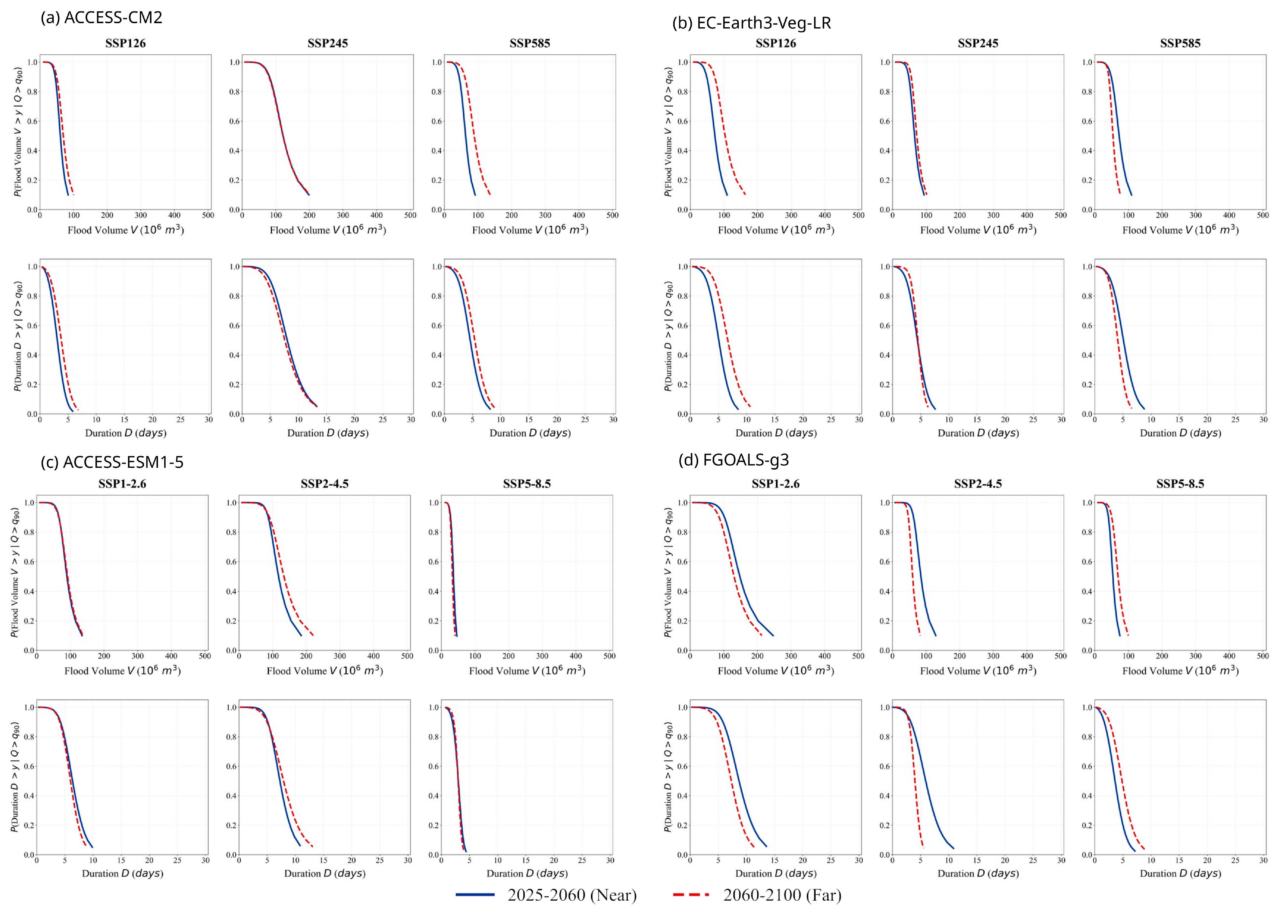
Figure 9 illustrates the conditional probability responses under extreme peak-flow conditions. Given that peak flow exceeds the 90th-percentile threshold, the probability of simultaneously high flood volume or long duration increases under high-emission scenarios. Under SSP585, the conditional probability of high flood volume increases from 0.23 under SSP126 to 0.56, while the probability of long flood duration increases from 0.18 to 0.45. These results indicate that climate change may enhance tail dependence among flood variables, highlighting the need to consider multivariate joint probability rather than only univariate peak-flow frequency.

4. Discussion

4.1. Model Performance

The results show that PXB-BVC improves runoff simulation compared with SWAT, HBV, and MPM. This improvement can be attributed to the integration of complementary process information from SWAT and HBV, nonlinear error correction by XGBoost, and calibration-period BMA weighting. SWAT, HBV, and MPM preserve hydrological process information but tend to underestimate some high-flow magnitudes. XGBoost can learn nonlinear residual patterns from calibration data, while BMA balances the two coupled branches according to their calibration-period posterior weights. This explains the reduced PBIAS values of 0.91% during calibration and 1.79% during validation.
This finding is consistent with recent hybrid hydrological modeling studies showing that machine learning models can improve streamflow simulation when they are combined with process-based hydrological information. For example, Jin et al. coupled a remote sensing-enhanced SWAT model with BiLSTM and showed improved daily streamflow simulations [48]. Solanki et al. further demonstrated that post-processing multiple hydrological models with machine learning methods can improve streamflow prediction [49]. Similarly, Bhasme and Bhatia emphasized that combining hydrological model structure with data-driven learning can improve both interpretability and predictive performance [50]. Compared with these studies, the present framework does not rely on a single process-based model as the physical information source. Instead, SWAT and HBV are used to provide complementary process representations before XGBoost correction and BMA weighting [48].
To further assess whether the improvement is attributable only to the use of machine learning, an RF-based benchmark was developed using the same calibration–validation periods and an NRBO-based hyperparameter optimization strategy. During validation, the BMA-RF ensemble achieved NSE = 0.871 and RMSE = 14.72 m3/s, whereas PXB-BVC achieved NSE = 0.89 and RMSE = 11.03 m3/s. This comparison suggests that the improvement is not solely due to adding a machine learning algorithm, but is also related to the specific PXB-BVC architecture and calibration-period BMA weighting strategy. This is also consistent with Sattari et al., who showed that Bayesian and copula-embedded model averaging can improve streamflow prediction by reducing single-model dependence [19]. Nevertheless, the margin between PXB-BVC and BMA-RF is moderate, and the comparison should be interpreted as basin-specific evidence rather than universal superiority over all hybrid hydrological models.

4.2. Hydrological Mechanisms of Future Runoff and Flood-Risk Changes

The projected increase in runoff and compound flood risk under higher-emission scenarios can be interpreted through the hydrological response of the XXRB to intensified precipitation and altered evapotranspiration. Stronger greenhouse gas forcing can increase precipitation extremes and enhance runoff generation, thereby raising the probability that high peak flow, large flood volume, and long flood duration occur together. Similar mechanisms have been reported in recent climate-impact studies. Kim and Villarini found that higher-emission scenarios can lead to more extreme flooding, although regional differences remain substantial [51]. O’Shea et al. also showed that changes in rainfall intensity and catchment wetness are key drivers of future flood-risk changes [52]. Ionno et al. emphasized that flood volume is an important but often underrepresented metric in climate change flood assessment [53]. These studies support the interpretation that future flood risk should be evaluated not only by peak flow but also by flood volume and duration.
The revised bivariate return-period figures further clarify that future flood-risk interpretation depends on the joint-probability definition. For ACCESS-ESM1–5 under SSP245, OR-type return periods indicate a clearer increase in event frequency, with near-future 50-year events becoming approximately 31.9–47.7-year events in the late-century period. This suggests that flood events defined by the exceedance of at least one critical characteristic, such as peak flow, flood volume, or duration, may become more frequent by the late twenty-first century. By contrast, AND-type return periods show weaker and less consistent changes because they require simultaneous exceedance of both variables. This distinction is hydrologically meaningful: peak flow, flood volume, and duration do not necessarily increase at the same rate, and changes in their dependence structure can alter compound-risk estimates even when marginal flood characteristics change only moderately.
These results are consistent with recent compound-extreme and copula-based studies emphasizing the importance of dependence structures in multivariate flood-risk assessment. Subhadarsini et al. highlighted the need to account for dependence among correlated hydrological time series when analyzing compound extremes, while Khajehali et al. showed that copula-based multivariate flood-frequency analysis can capture climate change effects more effectively than univariate analysis [54,55]. However, the projected increase in runoff and flood risk is not strictly linear across all GCMs, SSPs, or joint risk definitions. The magnitude and statistical significance of runoff trends vary among climate models, and the revised Figure 7 and Figure 8 show that even the same 50-year reference event can lead to different late-century interpretations under AND and OR definitions. Therefore, future flood-risk assessment should account for climate-projection uncertainty, dependence-structure uncertainty, and the practical meaning of the selected joint return-period definition.

4.3. Uncertainty, Limitations, and Transferability

Several sources of uncertainty remain. First, the use of four GCMs captures only part of the inter-model spread. A larger CMIP6 ensemble could more comprehensively quantify projection uncertainty. Second, SDSM downscaling may introduce uncertainty, especially when local precipitation extremes are not fully represented by large-scale predictors. Third, hydrological model structures, calibrated parameters, machine learning inputs, and BMA weights can affect the simulated runoff series. Although PXB-BVC improves runoff simulation in this basin, the model has not yet been tested across a large sample of catchments. Therefore, its generality should be evaluated further. Fourth, the observed record is relatively short for estimating tail dependence and long return periods. Kendall’s tau and 100-year return-period estimates should therefore be interpreted as scenario-based results with sampling uncertainty. Fifth, land use was kept static using the year-2000 dataset, whereas future land-use change may alter infiltration, evapotranspiration, and runoff generation. This assumption may affect future runoff and flood-risk estimates, especially in basins experiencing rapid urbanization or vegetation change.
The PXB-BVC framework can be extended to other basins and future flood cases through site-specific recalibration. Local DEM, land-use, soil, meteorological, and observed runoff data are required to establish and calibrate the process-based models. SWAT and HBV should be recalibrated for the target basin, XGBoost correction models should be retrained using local model outputs and observations, and BMA weights should be re-estimated using calibration-period predictions and observations only. For future applications, locally downscaled climate projections can then be used to drive the recalibrated hydrological and XGBoost models, after which flood events can be extracted and bivariate copulas can be refitted. Therefore, the framework is transferable as a modeling workflow, but its parameters, machine learning relationships, BMA weights, and copula dependence structures should be recalibrated before application to other basins.
Overall, the revised discussion shows that the main contribution of this study is not the independent use of SWAT, HBV, XGBoost, BMA, or copula analysis, but the integration of these components into a workflow that links runoff prediction with future compound flood-risk assessment. The comparison with recent studies supports the value of hybrid hydrological modeling and multivariate flood-risk analysis, while the uncertainty analysis clarifies the limitations that should guide future applications.

5. Conclusions

This study developed a physics–XGBoost-based Bayesian model averaging with bivariate copulas (PXB-BVC) framework for runoff prediction and multivariate flood-risk assessment under climate change. The framework integrates SWAT, HBV, XGBoost, BMA, SDSM, and bivariate copulas to link climate-driven runoff simulation with compound flood-risk estimation in the Xiangxi River Basin.
The main findings are as follows. First, PXB-BVC improved daily runoff simulation compared with SWAT, HBV, MPM, and the RF-based benchmark, achieving NSE values of 0.95 during calibration and 0.89 during validation. Second, future runoff and flood characteristics generally increase from the near-term to the late-century period, especially under SSP585, although the magnitude and statistical significance of these changes vary among GCMs. Third, the dependence among flood peak, flood volume, and flood duration remains positive but exhibits non-stationary changes under future climate forcing, indicating that flood-risk assessment should consider multivariate joint probability rather than relying only on univariate peak-flow analysis.
Overall, the PXB-BVC framework provides a useful workflow for improving runoff simulation and assessing non-stationary compound flood risk under future climate scenarios. However, the results should be interpreted in light of uncertainties related to GCM selection, SDSM downscaling, hydrological model structure, limited observed records, and static land-use assumptions. Future studies should test the framework in additional basins and incorporate larger climate-model ensembles and dynamic land-use scenarios.

Supplementary Materials

The following supporting information can be downloaded at https://www.mdpi.com/article/10.3390/rs18142275/s1.

Author Contributions

A.Y.: Conceptualization, Methodology, Data curation, Writing—review and editing, Visualization, Funding acquisition; W.L.: Conceptualization, Methodology, Data curation, Writing—original draft, Visualization, Software; P.G.: Resources, Data curation, Formal analysis, Writing—review and editing, Visualization; Y.F. and X.W.: Formal analysis, Validation. All authors have read and agreed to the published version of the manuscript.

Funding

This research was supported by the Science and Technology Planning Projects of Fujian Province (2025I0052) and the projects of Fujian Provincial Department of Finance (2025119-03).

Data Availability Statement

The raw data supporting the conclusions of this article will be made available by the authors on request.

Conflicts of Interest

The authors declare no conflicts of interest.

Abbreviation

AETActual Evapotranspiration
BMABayesian Model Averaging
CMIP6Coupled Model Intercomparison Project Phase 6
DEMDigital Elevation Model
GCMGlobal Climate Model
HBVHydrologiska Byrans Vattenbalansavdelning
HRUHydrological Response Unit
MPMMulti-Physics Model
NSENash–Sutcliffe Efficiency
NRBONewton–Raphson-Based Optimizer
PBMProcess-Based Model
PBIASPercent Bias
POTPeak-Over-Threshold
PXB-BVCPhysics–XGBoost-Based Bayesian Model Averaging with Bivariate Copulas
RFRandom Forest
RMSERoot Mean Square Error
SBMStatistical-Based Model
SDSMStatistical Downscaling Model
SSPShared Socioeconomic Pathway
SWATSoil and Water Assessment Tool
XXRBXiangxi River Basin

References

  1. Calvin, K.; Dasgupta, D.; Krinner, G.; Mukherji, A.; Thorne, P.W.; Trisos, C.H.; Romero, J.; Aldunce, P.; Barrett, K.; Blanco, G.D.; et al. IPCC, 2023: Climate Change 2023: Synthesis Report. Contribution of Working Groups I, II and III to the Sixth Assessment Report of the Intergovernmental Panel on Climate Change; Core Writing Team, Lee, H., Romero, J., Eds.; IPCC: Geneva, Switzerland, 2023. [Google Scholar]
  2. Vieira, M.J.F.; Stadnyk, T.A. Leveraging global climate models to assess multi-year hydrologic drought. npj Clim. Atmos. Sci. 2023, 6, 179. [Google Scholar] [CrossRef]
  3. He, J.; Lu, K.; Fosu, B.; Fueglistaler, S.A. Diverging hydrological sensitivity among tropical basins. Nat. Clim. Change 2024, 14, 623–628. [Google Scholar] [CrossRef]
  4. Tian, L.; Guo, S.; Feng, J.; He, C. Quantifying the altitudinal response of water yield capacity to climate change in an alpine basin on the Tibetan Plateau through integrating the WRF-Hydro and Budyko framework. Catena 2024, 242, 108087. [Google Scholar] [CrossRef]
  5. Naseri, K.; Hummel, M. A Bayesian Copula-Based Nonstationary Framework for Compound Flood Risk Assessment along US Coastlines. J. Hydrol. 2022, 610, 128005. [Google Scholar] [CrossRef]
  6. Liu, W.; Wu, J.; Xu, F.; Mu, D.; Zhang, P. Modeling the effects of land use/land cover changes on river runoff using SWAT models: A case study of the Danjiang River source area, China. Environ. Res. 2023, 242, 117810. [Google Scholar] [CrossRef] [PubMed]
  7. Liu, Y.R.; Li, Y.; Ma, Y.C.; Jia, Q.; Su, Y.Y. Development of a Bayesian-copula-based frequency analysis method for hydrological risk assessment—The Naryn River in Central Asia. J. Hydrol. 2020, 580, 124349. [Google Scholar]
  8. Kiran, K.S.G.; Srinivas, V.V. Multivariate Regional Frequency Analysis Using Conditional Extreme Values Approach. Water Resour. Res. 2022, 58, e2021WR031095. [Google Scholar] [CrossRef]
  9. Huang, X.; Yin, J.; Slater, L.J.; Kang, S.; He, S.; Liu, P. Global Projection of Flood Risk With a Bivariate Framework Under 1.5–3.0 °C Warming Levels. Earth’s Future 2024, 12, e2023EF004312. [Google Scholar] [CrossRef]
  10. Deng, C.; Sun, P.; Yin, X.; Zou, J.; Wang, W. Assessment of monthly runoff simulations based on a physics-informed machine learning framework: The effect of intermediate variables in its construction. J. Environ. Manag. 2024, 362, 14. [Google Scholar] [CrossRef]
  11. Nguyen, H.H.; Peters, K.; Kiesel, J.; Welti, E.A.R.; Gillmann, S.M.; Lorenz, A.W.; Jähnig, S.C.; Haase, P. Stream macroinvertebrate communities in restored and impacted catchments respond differently to climate, land-use, and runoff over a decade. Sci. Total Environ. 2024, 929, 172659. [Google Scholar] [CrossRef] [PubMed]
  12. Wei, Q.; Chen, P.; Jia, Z.; Chen, Y.; Yuan, Z.; Zhang, H.; Yang, J.; Niu, B.; Xu, Z. Exploring the influence of hydrological indicators on flow regimes through a data-driven modeling approach in the Huai River Basin, China. Environ. Res. 2025, 285, 122605. [Google Scholar] [CrossRef] [PubMed]
  13. Saxton, K.E.; Rawls, W.J. Soil Water Characteristic Estimates by Texture and Organic Matter for Hydrologic Solutions. Soil Sci. Soc. Am. J. 2006, 70, 1569–1578. [Google Scholar] [CrossRef]
  14. Giglou, A.N.; Nazari, R.; Karimi, M.; Museru, M.L.; Opare, K.N.; Nikoo, M.R. Future eco-hydrological dynamics: Urbanization and climate change effects in a changing landscape: A case study of Birmingham’s river basin. J. Clean. Prod. 2024, 447, 21. [Google Scholar]
  15. Cai, Y.; Zhang, F.; Wang, J.S.C.J.A.W. Enhancing SWAT model with modified method to improve Eco-hydrological simulation in arid region. J. Clean. Prod. 2023, 403, 136891. [Google Scholar] [CrossRef]
  16. Sadayappan, K.; Keen, R.; Jarecke, K.M.; Moreno, V.; Nippert, J.B.; Kirk, M.F.; Sullivan, P.L.; Li, L. Drier streams despite a wetter climate in woody-encroached grasslands. J. Hydrol. 2023, 627, 130388. [Google Scholar] [CrossRef]
  17. Jin, X.; Jin, Y.; Du, K.; Mao, X.; Zheng, L.; Fu, D.; Qin, Y. Irrigation impacts on grassland hydrological regimes in an arid endorheic river basin. J. Hydrol. 2024, 631, 130843. [Google Scholar] [CrossRef]
  18. Ma, M.; Zhao, G.; He, B.; Li, Q.; Wang, Z. XGBoost-based method for flash flood risk assessment. J. Hydrol. 2021, 598, 126382. [Google Scholar] [CrossRef]
  19. Sattari, A.; Jafarzadegan, K.; Moradkhani, H. Enhancing streamflow predictions with machine learning and Copula-Embedded Bayesian model averaging. J. Hydrol. 2024, 643, 131986. [Google Scholar] [CrossRef]
  20. Fei, K.; Du, H.; Gao, L. Accurate water level predictions in a tidal reach: Integration of Physics-based and Machine learning approaches. J. Hydrol. 2023, 622, 12. [Google Scholar] [CrossRef]
  21. Akbarian, M.; Saghafian, B.; Golian, S. Monthly streamflow forecasting by machine learning methods using dynamic weather prediction model outputs over Iran. J. Hydrol. 2023, 620, 129480. [Google Scholar] [CrossRef]
  22. Wu, H.; Zhang, J.; Bao, Z.; Wang, G.; Wang, W.; Yang, Y.; Wang, J. Runoff modeling in ungauged catchments using machine learning algorithm-based model parameters regionalization methodology. Engineering 2022, 28, 93–104. [Google Scholar] [CrossRef]
  23. Tang, Z.; Zhang, J.; Hu, M.; Ning, Z.; Shi, J.; Zhai, R.; Liu, C.; Zhang, J.; Wang, G. Improving streamflow forecasting in Semi-Arid basins by combining data segmentation and Attention-Based deep learning. J. Hydrol. 2024, 643, 131923. [Google Scholar]
  24. Wu, J.; Wang, Z.; Dong, J.; Cui, X.; Tao, S.; Chen, X. Robust Runoff Prediction With Explainable Artificial Intelligence and Meteorological Variables From Deep Learning Ensemble Model. Water Resour. Res. 2023, 59, e2023WR035676. [Google Scholar] [CrossRef]
  25. Szczepanek, R. Daily Streamflow Forecasting in Mountainous Catchment Using XGBoost, LightGBM and CatBoost. Hydrology 2022, 9, 226. [Google Scholar] [CrossRef]
  26. Wang, S.; Peng, H. Multiple spatio-temporal scale runoff forecasting and driving mechanism exploration by K-means optimized XGBoost and SHAP. J. Hydrol. 2024, 630, 130650. [Google Scholar]
  27. Kanani-Sadat, Y.; Safari, A.; Nasseri, M.; Homayouni, S. A novel explainable PSO-XGBoost model for regional flood frequency analysis at a national scale: Exploring spatial heterogeneity in flood drivers. J. Hydrol. 2024, 638, 131493. [Google Scholar] [CrossRef]
  28. Sezen, C.; Šraj, M. Improving the simulations of the hydrological model in the karst catchment by integrating the conceptual model with machine learning models. Sci. Total Environ. 2024, 926, 171684. [Google Scholar] [CrossRef] [PubMed]
  29. Yang, H.; Zhang, Z.; Liu, X.; Jing, P. Monthly-scale hydro-climatic forecasting and climate change impact evaluation based on a novel DCNN-Transformer network. Environ. Res. 2023, 236, 116821. [Google Scholar] [PubMed]
  30. Wang, S.; Liu, Y.; Wang, W.; Zhao, G.; Liang, H. Interpretable machine learning guided by physical mechanisms reveals drivers of runoff under dynamic land use changes. J. Environ. Manag. 2024, 367, 121978. [Google Scholar] [CrossRef]
  31. Xu, C.; Zhong, P.-a.; Zhu, F.; Xu, B.; Wang, Y.; Yang, L.; Wang, S.; Xu, S. A hybrid model coupling process-driven and data-driven models for improved real-time flood forecasting. J. Hydrol. 2024, 638, 131494. [Google Scholar]
  32. Jeong, H.; Lee, B.; Kim, D.; Qi, J.; Lim, K.J.; Lee, S. Improving estimation capacity of a hybrid model of LSTM and SWAT by reducing parameter uncertainty. J. Hydrol. 2024, 633, 15. [Google Scholar] [CrossRef]
  33. Guo, J.; Liu, Y.; Zou, Q.; Ye, L.-P.; Zhu, S.; Zhang, H. Study on optimization and combination strategy of multiple daily runoff prediction models coupled with physical mechanism and LSTM. J. Hydrol. 2023, 624, 129969. [Google Scholar] [CrossRef]
  34. Li, G.; Liu, Z.; Zhang, J.; Han, H.; Shu, Z. Bayesian model averaging by combining deep learning models to improve lake water level prediction. Sci. Total Environ. 2023, 906, 167718. [Google Scholar] [CrossRef] [PubMed]
  35. Moknatian, M.; Mukundan, R. Uncertainty Analysis of Streamflow Simulations Using Multiple Objective Functions and Bayesian Model Averaging. J. Hydrol. 2022, 617, 128961. [Google Scholar] [CrossRef]
  36. Wei, L.; Jiang, S.; Dong, J.; Ren, L.; Liu, Y.; Zhang, L.; Wang, M.; Duan, Z. Fusion of gauge-based reanalysis, and satellite precipitation products using Bayesian model averaging approach: Determination of the influence of different input sources. J. Hydrol. 2023, 618, 129234. [Google Scholar]
  37. Zhang, Q.; Li, Y.P.; Huang, G.H.; Wang, H.; Shen, Z. Bayesian analysis of variance for quantifying multi-factor effects on drought propagation. J. Hydrol. 2024, 632, 130911. [Google Scholar] [CrossRef]
  38. Yu, Q.; Jiang, L.; Wang, Y.; Liu, J. Enhancing streamflow simulation using hybridized machine learning models in a semi-arid basin of the Chinese Loess Plateau. J. Hydrol. 2023, 617, 129115. [Google Scholar] [CrossRef]
  39. Yue, S.; Ouarda, T.B.M.J.; Bobée, B.; Legendre, P.; Bruneau, P. The Gumbel mixed model for flood frequency analysis. J. Hydrol. 1999, 226, 88–100. [Google Scholar] [CrossRef]
  40. Ghorbel, A.; Trabelsi, A. Energy portfolio risk management using time-varying extreme value copula methods. Econ. Model. 2014, 38, 470–485. [Google Scholar] [CrossRef]
  41. Plackett, R.L. A Class of Bivariate Distributions. Publ. Am. Stat. Assoc. 1965, 60, 516–522. [Google Scholar] [CrossRef]
  42. Li, Y.; Tao, H.; Su, B.; Kundzewicz, Z.W.; Jiang, T. Impacts of 1.5 °C and 2 °C global warming on winter snow depth in Central Asia. Sci. Total Environ. 2019, 651, 2866–2873. [Google Scholar] [CrossRef] [PubMed]
  43. Salvadori, G.; Michele, C.D. Multivariate multiparameter extreme value models and return periods: A copula approach. Water Resour. Res. 2010, 46, 219–233. [Google Scholar] [CrossRef]
  44. Suo, N.; Xu, C.; Cao, L.; Song, L.; Lei, X. A copula-based parametric composite drought index for drought monitoring and applicability in arid Central Asia. Catena 2024, 235, 107624. [Google Scholar]
  45. Herath, H.M.V.V.; Chadalawada, J.; Babovic, V. Hydrologically Informed Machine Learning for Rainfall-Runoff Modelling: Towards Distributed Modelling. Hydrol. Earth Syst. Sci. 2020, 25, 4373–4401. [Google Scholar]
  46. Eingrüber, N.; Korres, W. Climate change simulation and trend analysis of extreme precipitation and floods in the mesoscale Rur catchment in western Germany until 2099 using Statistical Downscaling Model (SDSM) and the Soil & Water Assessment Tool (SWAT model). Sci. Total Environ. 2022, 838, 155775. [Google Scholar] [CrossRef] [PubMed]
  47. Yang, Z.Q.; Yang, A.L.; Zhou, X. Attributing terrestrial water storage changes on the Tibetan Plateau to climate and human drivers using a hybrid deep learning approach. J. Hydrol. 2026, 675, 135599. [Google Scholar] [CrossRef]
  48. Jin, L.; Xue, H.; Dong, G.; Han, Y.; Li, Z.; Lian, Y. Coupling the remote sensing data-enhanced SWAT model with the bidirectional long short-term memory model to improve daily streamflow simulations. J. Hydrol. 2024, 634, 131117. [Google Scholar]
  49. Solanki, H.; Vegad, U.; Kushwaha, A.; Mishra, V. Improving streamflow prediction using multiple hydrological models and machine learning methods. Water Resour. Res. 2025, 61, e2024WR038192. [Google Scholar] [CrossRef]
  50. Bhasme, P.; Bhatia, U. Improving the interpretability and predictive power of hydrological models: Applications for daily streamflow in managed and unmanaged catchments. J. Hydrol. 2024, 628, 130421. [Google Scholar]
  51. Kim, H.; Villarini, G. Higher emissions scenarios lead to more extreme flooding in the United States. Nat. Commun. 2024, 15, 237. [Google Scholar] [CrossRef] [PubMed]
  52. O’Shea, D.; Nathan, R.; Wasko, C.; Ho, M.; Sharma, A. Evaluation of key flood risk drivers under climate change using a bottom-up approach. J. Hydrol. 2024, 640, 131694. [Google Scholar] [CrossRef]
  53. Ionno, A.; Arsenault, R.; Troin, M.; Martel, J.-L.; Brissette, F. Impacts of climate change on flood volumes over North American catchments. J. Hydrol. 2024, 630, 130688. [Google Scholar] [CrossRef]
  54. Subhadarsini, S.; Kumar, D.N.; Govindaraju, R.S. A framework for multivariate analysis of compound extremes based on correlated hydrologic time series. J. Hydrol. 2024, 637, 131294. [Google Scholar] [CrossRef]
  55. Khajehali, M.; Safavi, H.R.; Nikoo, M.R.; Najafi, M.R.; Alizadeh-Sh, R. A copula-based multivariate flood frequency analysis under climate change effects. Sci. Rep. 2025, 15, 146. [Google Scholar] [CrossRef] [PubMed]
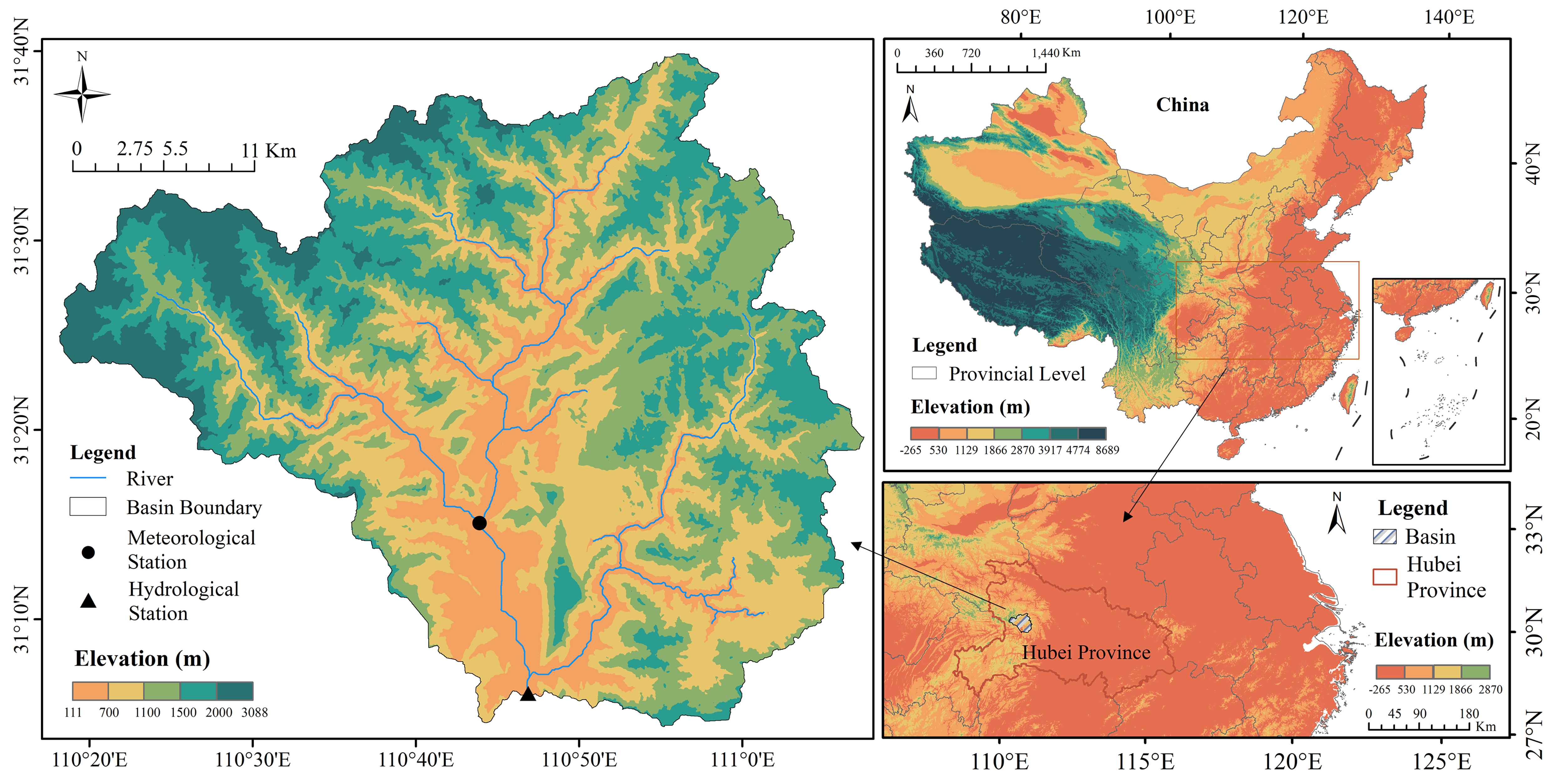
Figure 1. Location of the study area (Xiangxi River Basin) and distribution of hydrological and meteorological stations.
Remotesensing 18 02275 g001
Figure 2. Framework of the PXB-BVC model.
Remotesensing 18 02275 g002
Figure 3. Model performance evaluation: (a) daily simulated and observed runoff, (b) probability density distribution of daily runoff (dashed line represents the 99% quantile).
Remotesensing 18 02275 g003
Figure 4. Predicted monthly runoff under different climate scenarios.
Remotesensing 18 02275 g004
Figure 5. Median changes in flood peak, duration, and volume relative to the reference period (1993–2008) under different climate scenarios.
Remotesensing 18 02275 g005
Figure 6. Heatmaps of Kendall’s rank correlation coefficients for flood-characteristic pairs.
Remotesensing 18 02275 g006
Figure 7. Comparison of AND joint return periods for bivariate flood characteristics under SSP245 based on ACCESS-ESM1–5.
Remotesensing 18 02275 g007
Figure 8. Comparison of OR joint return periods for bivariate flood characteristics under SSP245 based on ACCESS-ESM1–5.
Remotesensing 18 02275 g008
Figure 9. Illustrates the evolution of conditional probabilities across different SSP scenarios.
Remotesensing 18 02275 g009
Table 1. Data sources and corresponding processing.
DataData SourcesResolutionsProcessing
2000 China land-use remote sensing monitoring data (LUCC)Institute of geographic sciences and natural resources research—CAS (http://www.resdc.cn, accessed on 23 January 2025)30 m × 30 mReclassify
DEM (digital elevation model) dataGeographical spatial data cloud website—CAS (http://www.gscloud.cn, accessed on 14 January 2025)30 m × 30 mHydrological model analysis
Spatial soil dataHarmonized world soil database
(https://www.fao.org, accessed on 26 January 2025)
1000 m × 1000 mHydrological model analysis
Meteorological data
(1991–2008)
Xingshan meteorological stationDaily-
Runoff data
(1993–2008)
Xingshan hydrological stationDaily-
Note: CAS represents Chinese Academy of Sciences; “-“ represents that no processing is required.
Table 2. The selected global climate models (GCMs) of CMIP6.
ModelCountryAbbreviationResolution
(Longitude × Latitude)
Time Periods
ACCESS-CM2AustralianM11.875° × 1.25°2025–2100
ACCESS-ESM1–5AustralianM21.875° × 1.25°2025–2100
EC-Earth3-Veg-LREuropean UnionM31.60° × 3.20°2025–2100
FGOALS-g3ChinaM42.00°  ×  2.25°2025–2100
Table 3. Model performance results for daily runoff.
ModelPeriodR2NSERMSEPBIAS
SWATcalibrated0.770.7414.24−9.73%
validated0.730.7213.71−9.45%
HBVcalibrated0.740.7214.71−12.35%
validated0.710.7116.24−16.30%
MPMcalibrated0.820.7918.73−15.67%
validated0.780.7615.37−16.58%
PXB-BVCcalibrated0.950.959.430.91%
validated0.890.8911.031.79%
Table 4. Results of Sen slope and M-K trend test for predicted runoff.
PeriodGCMClimate ScenariosSen Slope (m3·s−1·yr−1)Z-Valuep-ValueTrend Features
2025–2100ACCESS-CM2SSP1260.312.720.01Significant increase
SSP2450.161.420.16Non-significant increase
SSP5850.433.000.002Significant increase
ACCESS-ESM1–5SSP1260.131.370.17Non-significant increase
SSP2450.162.240.02Significant increase
SSP5850.465.080.01Significant increase
EC-Earth3-Veg-LRSSP1260.110.940.35Non-significant increase
SSP2450.450.390.69Non-significant increase
SSP5850.282.750.01Significant increase
FGOALS-g3SSP126−0.03−0.290.77Non-significant decrease
SSP2450.020.190.85Non-significant increase
SSP5850.282.830.004Significant increase
Table 5. Performance evaluation results of the copula functions.
Flood PairsGaussian CopulaStudent t CopulaFrank CopulaGumbel CopulaClayton Copula
BICRMSESEDBICRMSESEDBICRMSESEDBICRMSESEDBICRMSESED
P-V87.700.2912.97190.780.2922.98288.300.2912.96091.260.2963.05987.170.2762.668
P-D96.170.3153.47497.970.3183.54295.910.3173.52297.720.3223.63495.230.3013.161
V-D85.810.4045.70388.510.4045.70888.040.4045.71487.170.4055.74285.030.3845.164
Disclaimer/Publisher’s Note: The statements, opinions and data contained in all publications are solely those of the individual author(s) and contributor(s) and not of MDPI and/or the editor(s). MDPI and/or the editor(s) disclaim responsibility for any injury to people or property resulting from any ideas, methods, instructions or products referred to in the content.