Water Anomaly Type Identification Based on Deep Multisphere Decision Boundaries Using Remote Sensing Data

Highlights

What are the main findings?

• A deep multisphere decision boundaries (DMSDB) method is proposed to achieve unified and fine-grained identification of multiple water anomaly types.
• The model achieves high accuracy (F1 = 0.8789, mIoU = 0.7932), enabling classification of large-scale scenes (10,000 km²) within 33 s.

What are the implications of the main findings?

• The proposed method provides a practical solution for effective water anomaly monitoring under resource-constrained conditions.
• The multisphere decision boundary mechanism offers a generalizable paradigm for multiclass anomaly identification in remote sensing applications.

Abstract

The increasing frequency of water anomalies poses severe threats to aquatic ecosystem stability, water resource security, and socioeconomic sustainability. Rapid and accurate identification of these events is critical for early warning and informed environmental decision-making. However, existing type identification methods often fail to balance high precision with rapid inference since many depend on hand-crafted feature engineering or computationally intensive post-classification procedures that slow processing and increase confusion among anomalies with similar spectral characteristics. Therefore, in this study, a deep multisphere decision boundaries (DMSDB) method for unified, fine-grained identification of diverse water anomalies is developed. The method first involves constructing a compact 5-dimensional feature space by deriving physically interpretable indices from Sentinel-2 imagery. Then, a modified VM-UNet-v2 network is employed to extract water anomaly response features (WARFs) that capture the spatial–spectral characteristics of each anomaly. Finally, a multi-sphere-contrast loss function optimizes class-specific decision boundaries, compacting intraclass features while increasing the separation between spectrally similar anomaly categories. The validation results demonstrate that DMSDB achieves an average F1 score of 0.8789 and an mIoU of 0.7932, enabling efficient large-scale inference, and completing classification over a 10,000 km² scene within 33 s. These results highlight the method’s potential for effective or ground-based rapid environmental monitoring, supporting timely and category-specific responses to aquatic disturbances.

1. Introduction

The increasing frequency and diversity of water anomalies (e.g., floods, algal blooms, black-odor water, and offshore oil spills) pose significant threats to aquatic ecosystems, water security, and socioeconomic stability [1,2]. Rapid and accurate identification of these distinct anomaly types is therefore critical for enabling early warning and facilitating timely management responses, which rely on the intelligent detection of multicategory anomalies. However, achieving fast and reliable multi-type identification via satellite remote sensing remains challenging. Although these anomalies arise from distinct hydrological, biological, and chemical processes and are generally distinguishable in their spectral responses [3], similarities in spectral and radiometric characteristics may occur among different anomaly types as well as between anomalous and normal surface conditions under complex observation scenarios (e.g., mixed pixels, illumination variation, and background interference), thereby increasing the difficulty of accurate multi-class discrimination. Among various water anomalies, floods, algal blooms, black-odor water, and offshore oil spills are particularly representative due to their high occurrence frequency and significant environmental and socioeconomic impacts. The lack of a unified method that can maintain high discriminatory power therefore remains a key barrier to reliable, anomaly type identification.

Early research in this field focused primarily on water-quality parameter inversion and the retrieval of chlorophyll-a (Chl-a), total suspended matter (TSM), and colored dissolved organic matter (CDOM) from multispectral or hyperspectral imagery [4,5,6,7]. These parameters have proven valuable for assessing long-term ecosystem trends and evaluating water restoration policies. For instance, coastal transparency improved following the Bohai Sea Management Initiative [8]. Although parameter inversion methods have advanced substantially, they are designed primarily for continuous environmental assessment rather than the rapid detection of abrupt anomalies. The retrieval process typically requires atmospheric correction, bio-optical modeling, and empirical calibration, which increases the computational cost and hinders real-time application. Moreover, while these parameters reflect changes in water quality, they lack the categorical specificity required to discriminate among multiple surface anomaly types.

To improve responsiveness, spectral index-based methods have been developed for the fast empirical identification of specific anomaly types. These methods design algebraic combinations of spectral bands to amplify specific physical signals, such as water extent, vegetation, or turbidity, and have proven effective for single-type anomaly identification. For example, the normalized difference water index (NDWI) and the normalized difference built-up index (NDBI) are typically used to delineate flooded areas and urban inundation zones, respectively, whereas the normalized difference vegetation index (NDVI) and normalized difference chlorophyll index (NDCI) increase bloom identification by exploiting chlorophyll-related spectral peaks [9,10]. Black-odor water, characterized by high organic loading and low oxygen levels, has been studied using both field-derived and remote-sensing indices, such as the black and odds water quality index (BOWQI) and the remotely derived normalized difference black-odorous water index (NDBWI), which have achieved accuracies exceeding 80% across major Chinese cities [11,12]. To address the insufficient accuracy of existing remote sensing classification methods for surface water in complex backgrounds, a study proposes a novel water index (SSWI) [13] that integrates spectral and solar elevation angle dynamic variation characteristics based on GF-4 geostationary orbit satellite dense time-series imagery. Nevertheless, index-based approaches require substantial spectral prior knowledge and depend heavily on expert-driven index design. A single index typically corresponds to a single anomaly type, and multi-index combinations often lead to incompatibility among decision rules, degraded robustness, or conflicting anomaly indications. As a result, these methods are difficult to extend to consistent and accurate multitype identification in complex real-world environments.

Beyond empirical index approaches, recent advances in data-driven methods have improved the capacity for automated water anomaly type identification. Convolutional neural networks (CNNs), particularly U-Net architectures, have been widely adopted to integrate multisource inputs and learn spatial–spectral patterns directly from imagery. For instance, deep learning models such as U-Net have demonstrated superior performance in flood mapping from Sentinel-1 SAR imagery compared to traditional threshold-based methods and conventional machine learning approaches [14]. Furthermore, the integration of topographic variables, including slope, digital elevation models (DEM), and height above nearest drainage (HAND), has been shown to further improve classification accuracy in complex terrain conditions. Similar deep architectures have been extended to identify oil spills and flood susceptibility [15,16], often by coupling CNNs or recurrent models with optimization algorithms to increase generalizability and efficiency. Collectively, these studies demonstrate the growing potential of deep learning for multisource fusion and high-accuracy anomaly mapping. These models underscore the potential of deep architectures to automate water anomaly type identification and integrate multisource inputs. However, due to the potential for confusion between different types of water anomalies and between these anomalies and normal Earth’s surface spectral response characteristics, the class distributions of the model in the feature space may overlap, thus placing higher demands on the characterization of feature separability.

The emergence of decision boundary–based methods provide a potential direction for improving multiclass discrimination. A decision boundary defines regions in the feature space that correspond to different classes, and its structure directly influences the separability of feature distributions. By introducing explicit geometric constraints, such as hypersphere-based boundary modeling or margin-based separation, existing studies have shown that feature representations can be better organized, leading to improved intra-class compactness and inter-class separation [17,18]. These approaches suggest that explicitly structuring the feature space can help reduce ambiguity among classes and improve discrimination performance under complex data distributions. However, such strategies have not been specifically tailored to the task of multiclass water anomaly detection, where multiple anomaly types and normal Earth’s surface conditions coexist with varying degrees of spectral similarity.

Motivated by this perspective, this study proposes a deep multisphere decision boundary (DMSDB) method to enhance feature separability for multiclass water anomaly identification. The proposed method is inspired by Deep Multi-sphere Support Vector Data Description [19] and is adapted as a feature-space structuring strategy rather than a standalone classification method. By constructing water anomaly response features (WARFs) from five complementary indices (NDCI, NDTI, BOI, MNDWI, and NIR-SWIR), the method learns independent spherical decision regions for each anomaly category through a multisphere contrast loss. This design enables the feature space to be organized into relatively compact and separable regions corresponding to different anomaly types, thereby improving the model’s ability to distinguish among floods, algal blooms, black-odor water, and offshore oil spills. Nevertheless, the proposed method has certain limitations. First, its performance depends on the quality and representativeness of the selected spectral indices, which may affect its generalization across different sensors and environmental conditions. Second, the use of spherical decision boundaries assumes relatively compact feature distributions in the learned space, which may not fully capture highly complex or irregular structures. In addition, the current study is conducted on a limited number of annotated scenes, which may not fully capture the variability of water conditions across different regions and acquisition settings. However, the use of complementary feature representations partially alleviates the dependency on large-scale training data. These limitations will be further addressed in future work.

2. Data and Methodology

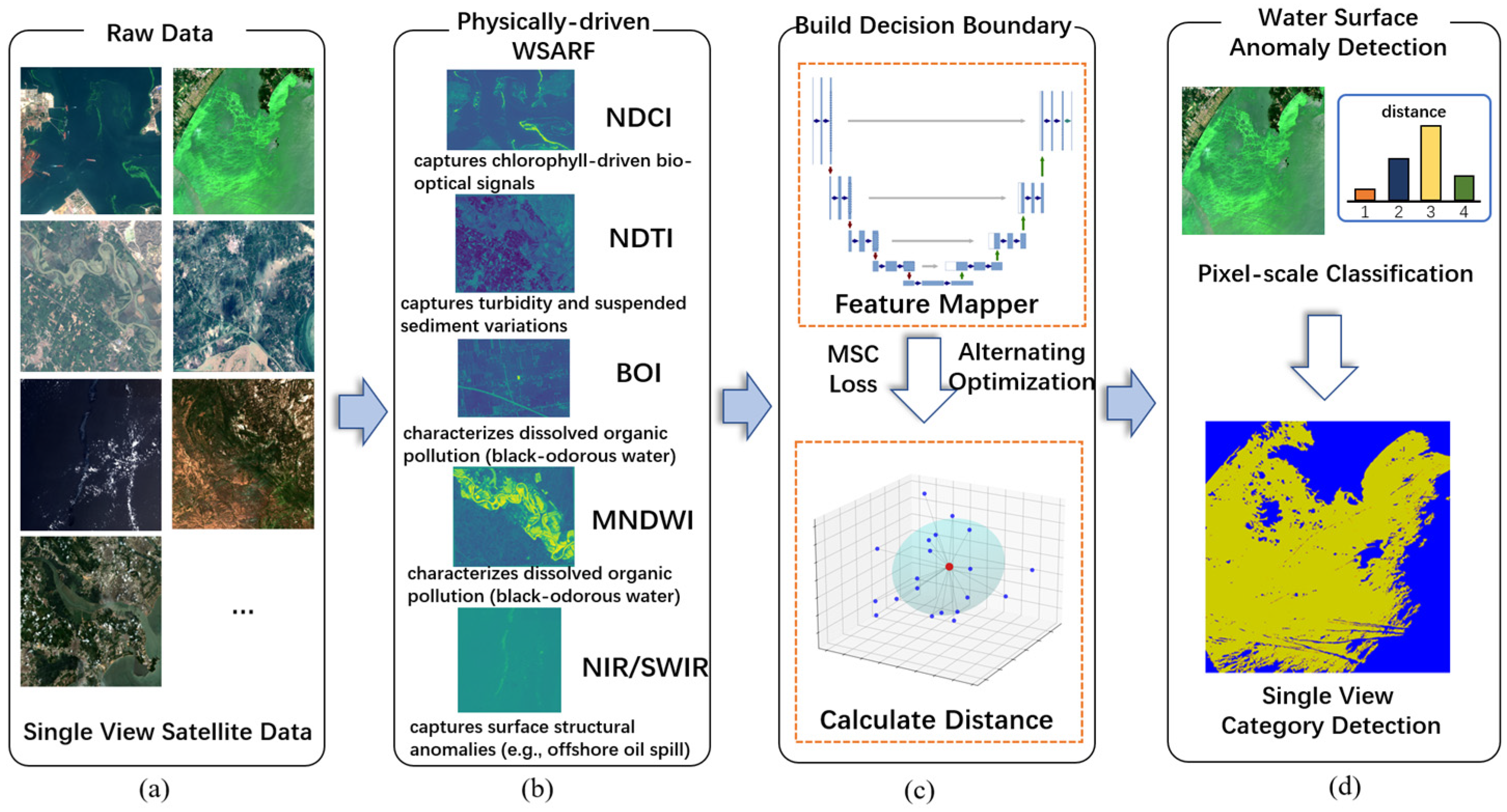
The methodology flowchart (Figure 1) provided here illustrates the DMSDB for water anomalies, a novel method designed for anomaly type identification utilizing multidimensional feature spaces. The process commences with dual inputs: label data serving as the ground truth for model training and Sentinel-2 L2A all-band data acting as the initial water surface anomaly response feature (WARF) data. The WARF Mapper then embeds the input data into manageable patches, followed by a series of VSS blocks applied sequentially to extract and integrate features at various levels. Each VSS block is followed by a patch merging step to consolidate the extracted features. The semantics and detail infusion (SDI) module then synthesizes these features into a unified representation. Subsequent fusion blocks and ConvTranspose layers refine and upscale the feature maps, culminating in the generation of WARF data. The refined data are then utilized to determine the decision boundary, which is visualized through a distance heat map that delineates potential anomalies. The final prediction result is a map indicating detected anomalies, demonstrating the model’s ability to perform efficient anomaly type identification. This architecture successfully addresses the computational complexity issues of existing methods, making it highly suitable for environments with limited computational resources and stringent response time requirements.

2.1. Data and Preprocessing

2.1.1. Data

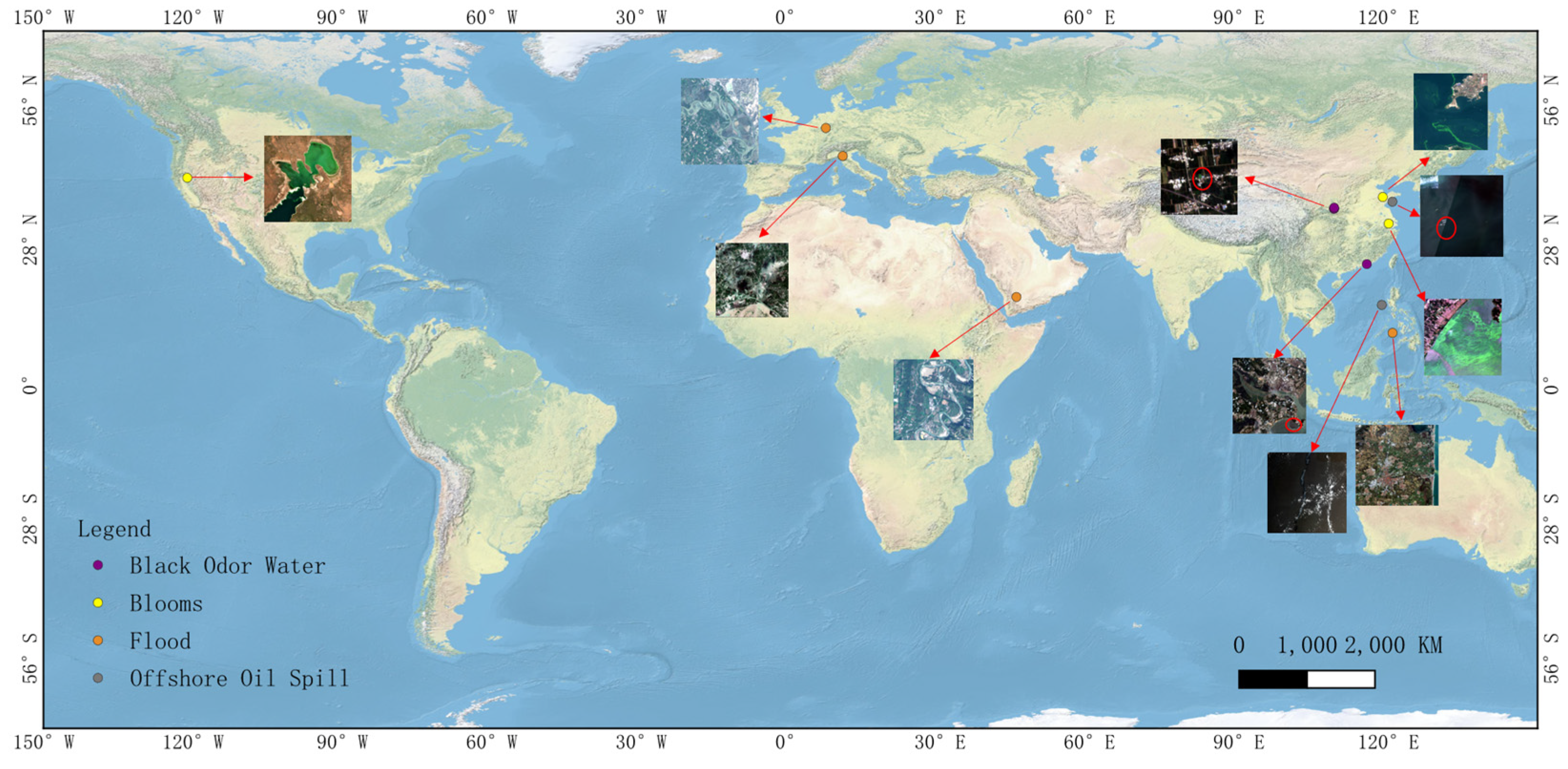
An evaluation was conducted on a curated Sentinel-2 dataset designed to assess the proposed method’s ability to identify multiclass water anomaly types. Figure 2 illustrates the geographic distribution of all selected study areas. Red circles are added to highlight the approximate locations of the anomalies for visualization, as the affected areas are relatively small at this map scale. 18 L2A scenes were selected, covering two independently verified cases for each of the four representative anomaly types—flood, algal bloom, black-odor water, and offshore oil spill—and 4 additional scenes were sampled from the surface of normal earth, which correspond to hydrological, biological, chemical, and petrochemical surface disturbances. To provide a spectral baseline, additional normal earth surface samples were randomly drawn across multiple regions rather than from fixed sites, ensuring broad coverage of non-anomalous conditions. These samples included forests, natural water bodies, grasslands, built-up areas, and bare soils, representing the dominant land-cover categories in the Sentinel-2 imagery. The combined dataset spans multiple continents (Asia and Europe) and diverse inland and coastal environments between 2019 and 2025. All scenes were cloud-free and preprocessed to Level-2A surface reflectance to ensure radiometric consistency.

Table 1. Sentinel-2 data acquiring time and location information of the selected data.

Anomaly Type	Acquiring Time	Location	Position
Flood	30 January 2022	Germany	7.121°E and 50.553°N
Flood	12 February 2020	Viadana, Lombardy	10.521°E and 44.927°N
Flood	8 April 2021	Indonesia	120.9°E and 9.4°S
Flood	25 November 2019	Madagascar	45.4°E and 16.6°S
Algal Bloom	10 July 2019	Shandong, China	118.951°E and 36.692°N
Algal Bloom	27 July 2022	Jiangsu, China	120.146°E and 31.357°N
Algal Bloom	2 August 2020	Califonia, USA	121.120°W and 40.558°N
Algal Bloom	3 May 2020	Jiangsu, China	120.092°E and 31.202°N
Black-odor Water	20 August 2020	Guangdong, China	115.757°E and 23.224°N
Black-odor Water	1 July 2024	Shannxi, China	109.201°E and 34.549°N
Black-odor Water	1 July 2024	Shannxi, China	109.139°E and 34.346°N
Black-odor Water	1 July 2024	Shannxi, China	109.200°E and 34.548°N
Offshore Oil Spill	19 April 2025	West Philippine Sea	118.766°E and 15.028°N
Offshore Oil Spill	27 April 2021	Shandong, China	120.889°E and 35.756°N
Normal Earth’s Surface	14 February 2024	Siberia, Russia	99.836°E and 55.347°N
Normal Earth’s Surface	20 May 2024	Papua, Indonesia	141.611°E and 0.437°N
Normal Earth’s Surface	3 August 2024	Qinghai, China	95.183°E and 37.247°N
Normal Earth’s Surface	18 October 2024	Hanoi, Vietnam	105.834°E and 21.027°N

summarizes the acquisition details, including the time, location, and central geographic coordinates of each water surface anomaly.

A patch-based learning strategy is adopted to provide spatially consistent local representations and to facilitate effective convolutional feature learning. Each full-resolution scene is subdivided into non-overlapping 128 × 128 pixel patches, which provide sufficient local spatial context for distinguishing water anomaly types while maintaining computational efficiency. The choice of patch size is motivated by the localized nature of water anomaly spectral responses, where discriminative information is primarily determined by nearby hydrological and surface conditions, and distant spatial context contributes limited additional discriminative value. This process not only increased the number of training samples but also provided spatially coherent contexts ideal for convolutional feature learning. It is worth noting that the diversity of the dataset is primarily ensured by the inclusion of scenes from different regions, acquisition times, and environmental conditions, rather than by the number of patches alone. The resulting patches were rigorously partitioned into training, validation, and test sets at a ratio of 7:2:1. Crucially, to prevent data leakage and ensure a reliable evaluation of generalization ability, all patches derived from the same original Sentinel-2 scene were assigned exclusively to one of the three splits.

2.1.2. Data Preprocessing

A preprocessing pipeline was applied to transform the extracted patches into a format suitable for model training. All preprocessing and data augmentation procedures were implemented using Python-3.8.19 based image processing libraries. The pipeline included data normalization, targeted data augmentation, and efficient tensor conversion to ensure stable training and reproducibility.

To improve model robustness under limited scene availability, a set of spatial and spectral augmentation strategies was applied exclusively to the training data. Geometric transformations, including random horizontal and vertical flipping, 90-degree rotations, and slight spatial shifts, were used to enhance invariance to satellite observation geometry and spatial orientation. These augmentations increase sample diversity at the patch level but do not replace the diversity provided by independent scenes.

In addition, spectral and radiometric perturbations were introduced to simulate realistic environmental and sensor-related variations. These included brightness and contrast adjustments to account for illumination variability, as well as additive spectral noise to mimic fluctuations in reflectance measurements. Furthermore, several remote sensing–oriented noise patterns were incorporated, including stripe noise to simulate sensor-induced artifacts, localized occlusions to represent partial observation interference, and Gaussian noise to approximate sensor noise. These augmentations were designed to improve the model’s generalization ability while preserving the physical consistency of spectral features.

For validation and testing, only minimal preprocessing was applied without augmentation to ensure an unbiased evaluation. This strategy ensures that performance metrics reflect the true generalization capability of the model rather than the effects of augmented data.

2.2. The Proposed Method

To improve the discriminability of different water anomaly types, this study employs a neural network–based feature mapper to transform the original response features into a structured feature space with enhanced separability. This mapping process explicitly reorganizes the feature distribution by increasing intra-class compactness and enlarging inter-class margins, thereby improving the distinction among multiple anomaly types as well as between anomalous and normal Earth’s surface conditions.

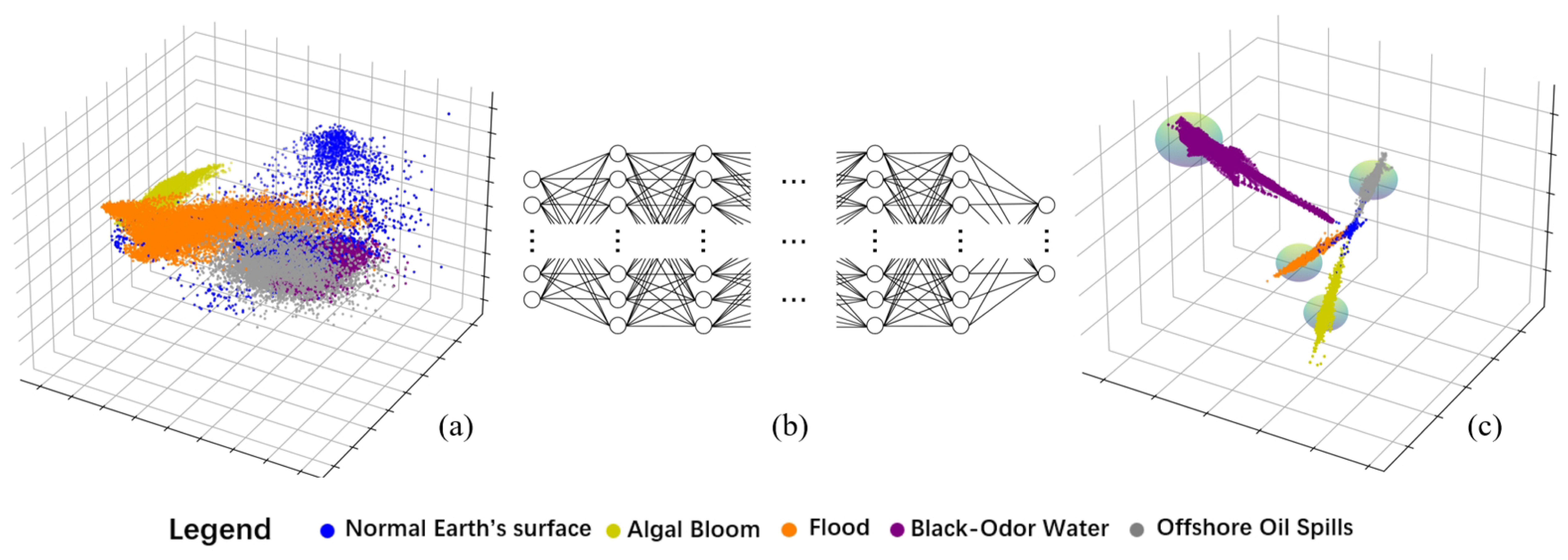
As illustrated in Figure 3, Figure 3a presents the initial response feature space, where samples from different categories exhibit relatively mixed distributions with unclear boundaries. Figure 3b shows the learned feature mapper, which performs a nonlinear transformation to reorganize the feature distribution. After this mapping, Figure 3c depicts the resulting feature space, where intra-class samples become more compact and inter-class distances are enlarged, leading to clearer class boundaries and improved separability among multiple anomaly types. In Figure 3, different colors are used to represent normal surface conditions and various water anomaly types. Since the input features are five-dimensional, principal component analysis (PCA) is applied to project the feature space into a lower-dimensional space for visualization.

2.2.1. Multi-Index Feature Space Construction

To characterize the spectral response features of different types of water body anomalies, this study, based on the principles of water color remote sensing, selects various remote sensing indices derived from the spectral characteristics of water body anomalies to construct a multidimensional feature set. Given that different water body anomalies typically correspond to distinct dominant physical or biological processes, their spectral responses exhibit targeted variation characteristics in specific bands. This study selects relevant indices commonly used in the field of remote sensing to detect various types of water body anomalies for feature construction. Therefore, by selecting remote sensing indices with different functionalities, this approach achieves a combined characterization of multiple types of water body anomalies, enabling the feature space to cover the primary response characteristics of different anomaly types.

Each index corresponds to a different type of water body anomaly. For algal bloom anomalies, the Normalized Difference Chlorophyll Index (NDCI) is derived from the difference in reflectance between the red and near-infrared bands. By leveraging the absorption characteristics of chlorophyll-a in the red band and the enhanced reflectance in the near-infrared region, it is capable of responding to changes in chlorophyll concentration in water bodies. Studies have shown that the NDCI can be used to estimate chlorophyll-a concentrations in turbid, productive water bodies and can, to some extent, reflect changes in algal biomass; therefore, this index is primarily used for algal bloom identification [20]. For the detection of floods and changes in water body extent, the Normalized Turbidity Index (NDTI) and the Modified Normalized Difference Water Index (MNDWI) are commonly used remote sensing indices. NDTI is primarily used to characterize optical changes in water bodies caused by suspended particles. Studies indicate that water turbidity is mainly determined by suspended sediments and related particles; these substances alter the reflectance characteristics of water bodies by enhancing backscattering, thereby affecting remote sensing observations [21]. Therefore, NDTI can, to a certain extent, reflect the degree of water turbidity dominated by suspended particles. In scenarios such as floods and sediment disturbance, where there is a significant increase in suspended particles, the NDTI typically serves as a good indicator; however, for clear-water floods with low sediment content, its response may be relatively limited. By incorporating the shortwave infrared band, MNDWI effectively enhances water body information while suppressing background interference from structures, vegetation, and soil. Studies indicate that, compared to the traditional NDWI, MNDWI reduces interference from non-water targets under complex background conditions, thereby facilitating the extraction of water body boundaries. It is primarily used to characterize water body extent and its spatial variations [22]. For the identification of black and odorous water bodies, the Black and Odorous Water Body Index (BOI) can be used to distinguish them from normal land surfaces. Studies indicate that the reflectance of black and odorous water bodies varies relatively gradually across the green-to-red spectral bands, and their spectral profiles differ from those of normal land surfaces; this characteristic is closely related to the presence of dissolved organic matter and pollutants [23]. Therefore, the BOI primarily reflects the spectral response characteristics of water bodies after contamination and is suitable for detecting black and odorous water bodies. For the detection of oil spills on the sea surface, the Normalized Difference Index (NIR-SWIR Index), constructed based on reflectance differences in the near-infrared and short-wave infrared bands, can effectively characterize the differences in reflectance and absorption between oil films and water bodies in the infrared bands. Previous studies have shown that the spectral response of oil films in the near-infrared and short-wave infrared regions differs significantly from that of water bodies; this combination of bands has been widely used to construct indices for oil spill detection and to identify oil pollution on the sea surface [24]. The aforementioned indices are complementary in their response mechanisms and can collectively characterize the spectral anomalies of different types of water. The indices are calculated as follows:

$$NDCI = (REDEDG{E}_1 - RED)/(REDEDG{E}_1 + RED)$$

(1)

$$NDTI=(RED-GREEN)/(RED+GREEN)$$

(2)

$$BOI=(GREEN-RED)/(RED+BLUE+GREEN)$$

(3)

$$MNDWI=(GREEN-SWI{R}_1)/(GREEN+SWI{R}_1)$$

(4)

$$NIR-SWIR Index=(NIR-SWI{R}_2)/(NIR+SWI{R}_2)$$

(5)

where $BLUE$ is the B2 band of Sentinel-2; $GREEN$ is the B3 band of green light; $RED$ is the B4 band; $REDEDG{E}_1$ is the B5 band; $NIR$ is the B8 band; $SWI{R}_1$ is the B11 band; and $SWI{R}_2$ is the B12 band.

2.2.2. Deep Multisphere Decision Boundaries Method

Conventional water analysis methods typically rely on a single decision boundary or unified detection rule, which is insufficient for distinguishing among multiple anomaly categories. Such approaches are not designed to resolve the spectral and spatial differences among floods, algal blooms, black-odor water, and oil spills or to provide the category-level discrimination required in operational settings.

To overcome this limitation, a deep multisphere decision boundaries (DMSDB) method is proposed. The core idea is to allocate an independent, minimal sphere for each specific anomaly class within the learned feature space. This transforms the task from a binary anomaly detection problem into a fine-grained, multiclass recognition problem. As illustrated in Figure 3c, our goal is to map the features of each anomaly subtype into a compact cluster around its own sphere center while simultaneously maximizing the margin between different spheres. This structured feature space enables explicit discrimination among the four target anomaly types, moving beyond mere detection to precise identification.

The foundation of this discriminative feature space is constructed by a dedicated neural network mapper, whose architecture is inspired by the VM-UNetV2 model [25]. The mapper comprises two distinct stages: the WARF Extract Stage and the Universal Indices Extract Stage. Given an input image $I$, where $I$ is a matrix of dimensions $H\times W\times 5$, the RS Indices Extractor generates a set of features $F$, which is also a matrix of dimensions $H\times W\times 5$. Subsequently, the universal indices extractor produces multi-level feature representations based on $F$, where the features at the $i_{th}$ level are denoted as $f_i^o$. The accumulated features, represented as {$f_1^o,f_2^o,\dots ,f_M^o$}, are subsequently forwarded to the SDI [26] module for further enhancement. The channel of $\mathrm{f}$ is $2^i\times C$. The set {$f_1^o,f_2^o,\dots ,f_M^o$} is collectively entered into the SDI module for feature fusion. In this context, $f_i$ corresponds to $f_i^{\prime }$, whose dimensions are ${\displaystyle \frac{H}{2^{i+1}}}\times {\displaystyle \frac{W}{2^{i+1}}}\times 2^{i}C$. This study employs [$N_1,N_2,N_3{,N}_4$] VSS blocks across the four stages of the extractor, with the channel counts for each stage being $[C, 2C, 4C, 8C]$, respectively.

The VSS block is derived from VMamba and represents the fundamental component of the encoder. The input is initially processed through a linear embedding layer, after which it is divided into two separate information streams. One stream is directed through a 3 × 3 depthwise convolution layer [27] and subsequently a Silu activation function before it enters the main 2D-Selective-Scan (SS2D) module. The SS2D output is subsequently subjected to a layer normalization layer and combined with the output from the other information stream, which has also undergone a Silu activation. This merged output represents the final result of the VSS block.

In the SDI module, with the hierarchical feature maps $f_i^0={\displaystyle \frac{H}{2^{i+1}}}\times {\displaystyle \frac{W}{2^{i+1}}}\times 2^{i}C$, $1\le i\le 4$ is generated by the encoder, where i represents the $i_{th}$ level. Following UNetV2 [26], the CBAM [28] is employed to implement spatial and temporal attention. The calculation formula is as follows, where ${\Phi }_i^{attention}$ represents the $i_{th}$ attention:

$$f_i^1={\Phi }_i^{attention}\left(f_i^0\right)$$

(6)

A 1 × 1 convolution is then applied to align the channel of $f_i^1$ to c, and the resulting feature map is represented as $f_i^2\in R^{H_i\times W_i\times c}$.

Next, at each decoder level $i$, $f_i^2$ is used as the target reference. The feature maps at every $j_{th}$ level are resized to match the same resolution as $f_i^2$, formulated as follows:

$$f_{ij}^3=\left\{\begin{array}{c}D\left(f_j^2, \left(H_i, W_i\right)\right) if j<i,\\ I\left(f_j^2\right) if j=i,\\ U\left(f_j^2, \left(H_i, W_i\right)\right) if j>i,\end{array}\right.$$

(7)

where $D, I$, and $U$ represent adaptive average pooling, identity mapping, and bilinearly interpolating $f_j^2$ to the resolution of $H_i$ × $W_i$, respectively, with $1\le i, j\le M$.

$$f_{ij}^4={\theta }_{ij}\left(f_{ij}^3\right)$$

(8)

$$f_i^5=H\left(\left[f_{i1}^4,f_{i2}^4,f_{i3}^4,f_{i4}^4\right]\right)$$

(9)

In this context, ${\theta }_{ij}$ represents the parameters of the smooth convolution, whereas $f_{ij}^4$ denotes the $j_{th}$ smoothed feature map at the $i_{th}$ level. Here, $H\left(\right)$ represents the Hadamard product. Subsequently, the value of $f_i^5$ is transmitted to the decoder at the $i_{th}$ level, where it is used to reconstruct the image in greater detail and to perform further segmentation.

2.2.3. Multisphere Contrast Loss

Learning the multisphere decision boundary requires a specialized objective function. A MultiSphere Contrast Loss (MSC loss) is proposed, which simultaneously learns the parameters of the feature mapping network as well as the optimal centers and radii of multiple spheres. The MSC loss function is as follows:

$${\mathcal{L}}_{\mathrm{total}}={\mathcal{L}}_{\mathrm{attract}}+\lambda {\mathcal{L}}_{\mathrm{repel}}$$

(10)

$${\mathcal{L}}_{\mathrm{attract}}={\displaystyle \frac{1}{N}}{\displaystyle \sum _{i=1}^N}{w}_{y_i}\cdot A\left(\right|f(x_i)-c_{y_i}{|}^2)$$

(11)

$${\mathcal{L}}_{\mathrm{repel}}=-{\displaystyle \frac{1}{\left|\mathcal{K}\right|}}\sum _{k\in \mathcal{K}}{\displaystyle \frac{1}{\left|S_k\right|}}\sum _{x_i\in S_k}\mathrm{l}\mathrm{o}\mathrm{g}(1-e^{-A(\underset{j\ne k}{min}|f(x_i)-c_j{|}^2)}+ϵ)$$

(12)

where $f\left(x\right)$ is our feature mapper and $A\left(x\right)$ is the pseudo-huber loss [29]. The total loss ${\mathcal{L}}_{\mathrm{total}}$ consists of two key components: an attraction loss ${\mathcal{L}}_{\mathrm{attract}}$ and a repulsion loss ${\mathcal{L}}_{\mathrm{repel}}$, balanced by a weighting factor $\lambda$. The attraction loss ${\mathcal{L}}_{\mathrm{attract}}$ pulls samples toward their corresponding class centers $c_{y_i}$. It is computed as the weighted average of the Pseudo-Huber loss applied to the squared distance between each sample’s feature representation and its class center. Class-specific weights $w_{y_i}$ are incorporated to handle potential class imbalance. The repulsion loss ${\mathcal{L}}_{\mathrm{repel}}$ pushes samples away from the centers of other classes. It uses a negative log transformation over a smoothed minimum distance from sample features to all other class centers, also measured via the pseudo-Huber function. This encourages large interclass margins and reduces ambiguity near decision boundaries. The pseudo-Huber function is central to both terms. It provides quadratic behavior for small distances—ensuring stable gradient-based learning—and linear scaling for large distances, enhancing robustness to outliers. By jointly optimizing attraction and repulsion, this loss effectively shapes the feature space into well-separated yet compact spheres, enabling fine-grained multiclass anomaly type identification. The overall formulation is end-to-end differentiable and suitable for training deep feature mapping networks.

2.2.4. Multisphere Learning via Alternating Optimization

The algorithm for deep multisphere decision boundaries training embodies a novel approach designed to overcome the inherent limitations of conventional anomaly detection, particularly in achieving fine-grained discrimination among multiple subtypes within a broad anomaly category. Its operational logic is founded upon an alternating optimization strategy that iteratively refines two interrelated components: the structural boundaries defining each class in the feature space and the parameters of the deep feature extraction network. During the sphere parameter update phase, the network parameters remain fixed while the algorithm recalibrates the centroid and radius of each class-specific sphere on the basis of the distribution of real samples, ensuring that each sphere tightly encapsulates its designated anomaly subtype. This geometric structuring is counterbalanced by the network parameter update phase, where the sphere parameters are frozen and the feature extraction network is trained to optimize a multi-objective loss function. This composite loss function synergistically combines an attraction term, which draws samples toward their corresponding class centroids to enhance intraclass compactness, with a repulsion term that actively separates samples from all foreign class centers to maximize interclass separation. The repeated alternation between these two optimization stages allows the feature representation and the multisphere parameters to be progressively refined in a mutually reinforcing manner, enabling the learned embedding space to better capture the intrinsic distribution characteristics of each anomaly category. As training proceeds, samples belonging to the same class become increasingly concentrated around their corresponding sphere centers, while the feature distances between different categories are continuously enlarged. Meanwhile, the updated sphere parameters provide more accurate supervisory signals for subsequent feature learning, and the progressively optimized feature representations further improve the estimation of class centroids and sphere radii, forming a closed-loop optimization process. This iterative refinement mechanism effectively reduces feature ambiguity among confusing categories and enhances the robustness of the learned decision boundaries under complex data distributions. The interplay between these optimization phases facilitates the emergence of a highly discriminative feature space where different anomaly categories occupy distinct and well-separated regions. Consequently, this method transcends traditional binary anomaly detection by enabling precise multiclass recognition, ultimately offering a robust solution for complex surface anomaly detection scenarios requiring subtype differentiation.

The detailed training process of the proposed method is outlined in Algorithm 1, where the iterative optimization of the sphere parameters and network weights is presented in pseudo-code form.

Algorithm 1. Deep Multi-Sphere Decision Boundary Training

Input: Labeled dataset $D$ Number of classes $c$ Feature network $\phi$ Hyperparameter $\nu$ Learning rate $\alpha$ Output: Trained network ${\phi }^{*}$ Hypersphere centers {$C_1,C_2\dots ,C_c$} Radii {$R_1$,…, $R_c$} 1. Initialize the network parameters θ and hypersphere centers {ck}. 2. Initialize radii {$R_1$,…, $R_c$} ← 0.1. 3. For epoch = $1$ to $E$ do: 4.   Update hypersphere parameters periodically. 5.   For each class $k$: 6.     $D_k$ ←$\left\{\right|\left|\phi \right(x_i)-C_k|{|}^2| y_i=k\}$. 7.     $R_k$ ← quantile($D_k$, $1-\nu$). 8.   End For. 9.   For each mini-batch {($x_b,y_b$)} in $D$: 10.     $f_b$ ← $\phi \left(x_b\right)$. 11.     Compute ${\mathcal{L}}_{\mathrm{attract}}$ 12.     Compute ${\mathcal{L}}_{\mathrm{repel}}$. 13.     Compute ${\mathcal{L}}_{\mathrm{total}}$. 14.     Update $\theta$ ← $\theta -\alpha {\nabla }_{\theta }{\mathcal{L}}_{\mathrm{total}}$. 15.   End For. 16. End For. 17. Return ${\phi }^{*}$, {$C_k$}, and {$R_k$}.

3. Results and Analysis

All the experiments were implemented using the deep multisphere decision boundaries method. The model was trained with the VM-UNet-v2 architecture as the backbone feature extractor initialized using Xavier initialization and optimized using the Adam optimizer with an initial learning rate of 0.001 and a weight decay of $1\times {10}^{-5}$. Learning rate milestones were scheduled at epochs 50, 100, and 200 to ensure stable convergence across the 300 training epochs. The batch size was set to 128. To ensure reproducibility, a fixed random seed 42 was used. The method was configured with a feature space dimension of four corresponding to the 5 water anomaly indices ($NDCI$, $NDTI$, $BOI$, $MNDWI$ and $NIR-SWIR Index$) and a five-class classification setup, representing the four water anomaly types and an additional background class. The decision boundary strategy hyperparameter was set to ν = 0.1, balancing the one-class boundary constraint and the interclass repulsion term within the loss function. A block coordinate optimization strategy was adopted to alternately update the network parameters and sphere boundaries, with a warm-up period of 5 epochs and boundary updates performed every 5 epochs.

3.1. Quantitative Performance Evaluation

Table 2. F1 scores for the detection of different water anomalies (bold text indicates the best results).

Anomalies	$\mathit{\nu }$ = 0.1		$\mathit{\nu }$ = 0.05		$\mathit{\nu }$ = 0.01
	$\mathit{\lambda }$ = 0.1	$\mathit{\lambda }$ = 1	$\mathit{\lambda }$ = 0.1	$\mathit{\lambda }$ = 1	$\mathit{\lambda }$ = 0.1	$\mathit{\lambda }$ = 1
Flood	0.9428	0.9317	0.9492	0.9411	0.9447	0.9273
Algal Bloom	0.9467	0.9259	0.9581	0.9043	0.9635	0.9461
Black-Odor Water	0.5612	0.7257	0.8348	0.8536	0.8091	0.8170
Offshore Oil Spill	0.7359	0.7091	0.7735	0.7330	0.7876	0.7316
mIoU	0.7631	0.7676	0.7932	0.7594	0.7527	0.7547
Mean F1	0.7967	0.8231	0.8789	0.8580	0.8762	0.8555

summarizes the F1 scores of the proposed model for detecting four major water anomaly types—flood, algal bloom, black-odor water, and offshore oil spills—under different combinations of hyperparameters ν (0.1, 0.05, and 0.01) and λ (0.1 and 1). The results indicate that model performance is jointly influenced by both ν and λ, with λ = 0.1 generally yielding better detection accuracy across most anomaly categories.

For flood detection, the proposed model maintains consistently high performance across all parameter settings, with F1 scores ranging from 0.9273 to 0.9492. The best performance is achieved at ν = 0.05 and λ = 0.1, while only minor fluctuations are observed under different parameter combinations, demonstrating strong robustness of the model for flood detection. Algal bloom detection also achieves stable and high accuracy under all configurations, with F1 scores ranging from 0.9043 to 0.9635. The highest F1 score is obtained at ν = 0.01 and λ = 0.1. Moreover, under λ = 0.1, the performance gradually improves as ν decreases, indicating that relatively tighter boundary constraints help enhance the separability of algal bloom features in the latent feature space. Compared with floods and algal blooms, black-odor water detection exhibits stronger sensitivity to hyperparameter settings. When ν = 0.1 and λ = 0.1, the F1 score is only 0.5612, indicating insufficient discrimination capability under relatively loose boundary constraints. As ν decreases to 0.05, the performance improves significantly, reaching 0.8348 at λ = 0.1 and 0.8536 at λ = 1. However, when ν is further reduced to 0.01, the performance decreases slightly, suggesting that excessively tight boundary constraints may limit the representation of the complex spectral variability of black-odor water. For offshore oil spill detection, the model achieves relatively stable performance, with F1 scores ranging from 0.7091 to 0.7876. The best performance is achieved at ν = 0.01 and λ = 0.1. In addition, under λ = 0.1, the F1 score gradually increases as ν decreases, indicating that stronger boundary constraints are beneficial for capturing subtle spectral differences between oil spill regions and surrounding seawater. From an overall perspective, the best performance is achieved at ν = 0.05 and λ = 0.1, where the mean F1 score reaches 0.8789 and the mIoU reaches 0.7932, both representing the highest overall performance among all parameter combinations. These results indicate that a moderate boundary constraint combined with a lower interclass repulsion weight provides the most balanced feature representation for diverse water anomaly types. Therefore, the parameter combination ν = 0.05 and λ = 0.1 is selected as the optimal setting in this study due to its superior and consistent performance across multiple evaluation metrics.

3.2. Qualitative Analysis of Detection Results

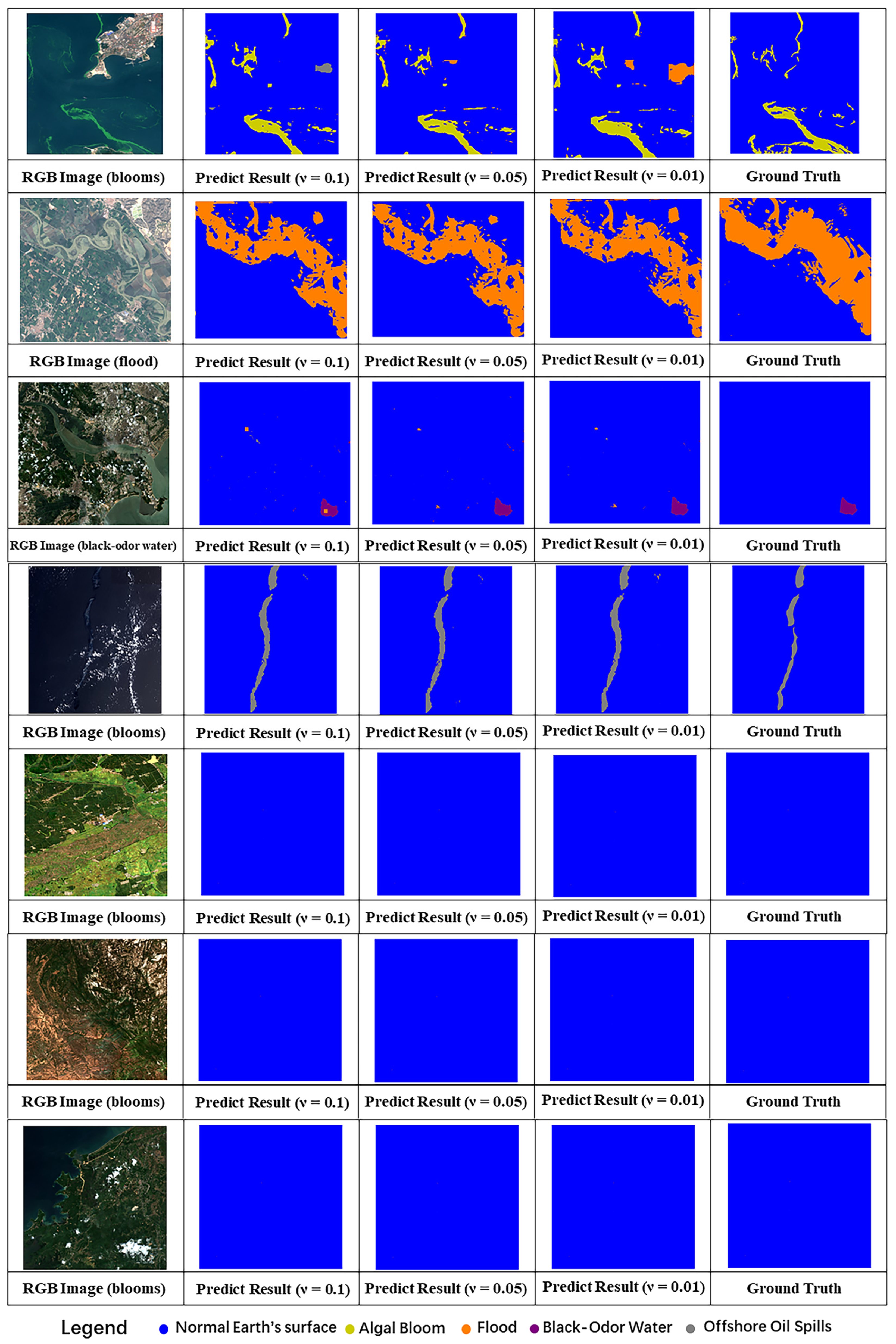
Figure 4 provides qualitative examples of detection outputs under different decision boundary parameter settings. Across all tested values of ν (0.1, 0.05, and 0.01), the predicted anomaly maps exhibit consistent spatial patterns and show strong agreement with the ground truth annotations, indicating that the proposed method maintains stable detection capability over a wide range of decision boundary configurations. Although slight variations can be observed in the predicted boundary details, the overall anomaly regions and category distributions remain highly consistent. These results further demonstrate the robustness of the proposed method and suggest that its detection performance is relatively insensitive to moderate changes in the decision boundary parameter.

Across all anomaly categories, the predicted maps are generally consistent with the reference annotations; however, a limited and acceptable level of cross-class misclassification is still observed, reflecting the robustness of the proposed multisphere decision boundary strategy across different parameter settings. Overall, ν = 0.05 provides the most balanced detection performance by maintaining target integrity while preserving boundary accuracy. In contrast, ν = 0.1 tends to produce under-segmentation due to relatively loose boundary constraints, whereas ν = 0.01 is more susceptible to over-segmentation and boundary diffusion caused by excessively compact feature boundaries. For algal bloom events, all parameter settings successfully identify the primary anomalous regions, indicating that the proposed framework is highly sensitive to chlorophyll-induced spectral anomalies. Nevertheless, ν = 0.01 introduces more pronounced cross-class confusion, with portions of bloom regions being misclassified as flood anomalies. In flood scenarios, the model accurately captures the major inundated areas under all parameter settings, while ν = 0.05 achieves superior spatial continuity and boundary completeness. By comparison, ν = 0.1 fails to detect certain marginal regions, and ν = 0.01 generates additional anomalous responses in localized areas. For black-odorous water, the model exhibits higher sensitivity to decision boundary configurations due to the small spatial extent and complex spectral characteristics of the targets. Specifically, ν = 0.1 results in noticeable false negatives, whereas ν = 0.05 and ν = 0.01 successfully identify the primary anomalous regions but still exhibit minor deviations in boundary delineation. In offshore oil spill cases, all parameter settings effectively capture the major pollution zones, while ν = 0.05 achieves a better trade-off between target completeness and false positive suppression. Furthermore, normal surface samples remain largely free from abnormal responses across all parameter settings, indicating that the proposed method possesses strong false positive suppression capability in non-anomalous regions.

In practical detection scenarios, the proposed algorithm demonstrates processing capabilities that are well aligned with the acquisition characteristics of Sentinel-2 imagery. Considering the satellite’s scene acquisition cycle of approximately 38 s and its spatial resolution of 10 m per pixel, the system employs a tile-based processing architecture that analyzes 128 × 128-pixel units in parallel during the data downlink process. Validation on a dataset comprising 1726 scenes confirms that the model maintains stable throughput, achieving an average inference time of 33.37 s on an NVIDIA V100 GPU (16 GB), indicating strong potential for onboard deployment. This architectural design effectively eliminates the processing bottleneck between the data acquisition and analysis phases.

3.3. Ablation Experiments

To systematically evaluate the contributions of input feature configuration, loss formulation, and decision boundary design, ablation experiments were conducted, as summarized in

Table 3. The detection of different water anomalies for ablation study (bold text indicates the best results).

Method	Input Features	Loss	Boundary	mIoU	mF1
UNet	RGB	Focal Loss	Softmax classfier	0.1356	0.2095
VMUNetV2	RGB	Focal Loss	Softmax classfier	0.1459	0.2376
DeepLabV3+	RGB	Focal Loss	Softmax classfier	0.1391	0.2135
VMUNetV2	NDCI, NDTI, BOI, MNDWI, NIR-SWIR	Focal Loss	Softmax classfier	0.1925	0.1957
One Index Input	MNDWI	MSC Loss	Multisphere	0.5481	0.5791
Attraction-only	NDCI, NDTI, BOI, MNDWI, NIR-SWIR	Attraction Loss	Multisphere	0.0000	0.0000
Ours	NDCI, NDTI, BOI, MNDWI, NIR-SWIR	MSC Loss	Multisphere	0.7920	0.8786

. For a fair comparison, all baseline models were trained under identical experimental settings. UNet and DeepLabV3+ were initialized with ImageNet pre-trained weights, whereas VMUNetV2 was initialized using Xavier initialization because no publicly available ImageNet pre-trained model is available for this architecture. All models were optimized using the Adam optimizer with an initial learning rate of 0.001 and a weight decay of $1\times {10}^{-5}$. The learning rate was decayed at epochs 50, 100, and 200 during a total of 300 training epochs with a batch size of 128. In addition, training and validation losses of all baseline models reached stable convergence before the end of the 300 training epochs. A fixed random seed of 42 was adopted throughout all experiments to ensure reproducibility.

Under identical training settings, all conventional semantic segmentation baselines exhibit limited performance when relying solely on RGB inputs. Specifically, UNet, VMUNetV2, and DeepLabV3+ achieve mIoU values of 0.1356, 0.1459, and 0.1391, respectively, with corresponding mF1 scores of 0.2095, 0.2376, and 0.2135. The relatively low performance of these RGB-based methods suggests that RGB information alone is insufficient to effectively characterize the spectral differences among multiple water anomaly categories, rather than reflecting limitations of the segmentation architectures themselves. Under this challenging multi-class water anomaly detection task, the lack of discriminative spectral information limits the effectiveness of architectural improvements, resulting in comparable performance among different segmentation backbones. Replacing RGB inputs with five remote sensing indices (NDCI, NDTI, BOI, MNDWI, and NIR-SWIR) while retaining the conventional softmax classifier improves the mIoU of VMUNetV2 from 0.1459 to 0.1925. However, the corresponding mF1 score remains relatively limited, indicating that enhanced spectral representations alone cannot fully resolve the complex feature distributions of multiple water anomaly categories when conventional softmax decision boundaries are employed.

Internal ablation experiments further demonstrate the effectiveness of the proposed method. When only a single spectral index (MNDWI) is provided, introducing the multisphere decision boundary together with the MSC loss already yields a substantial improvement, achieving an mIoU of 0.5481 and an mF1 score of 0.5791. This result indicates that the proposed geometric feature constraints can significantly enhance class discrimination even under limited spectral information. In contrast, removing the inter-class repulsion term and retaining only the attraction component causes feature collapse, resulting in mIoU and mF1 values of 0, which demonstrates that intra-class attraction alone cannot establish discriminative feature representations for multi-class water anomaly recognition. Finally, the complete method, integrating five remote sensing indices with the proposed MSC loss and multisphere decision boundary, achieves the best overall performance with an mIoU of 0.7920 and an mF1 score of 0.8786. These results confirm that the superior performance of the proposed method arises from the synergistic combination of enhanced spectral representation, discriminative feature optimization, and multisphere decision boundary construction.

3.4. Robustness Analysis via Random Seed Initialization

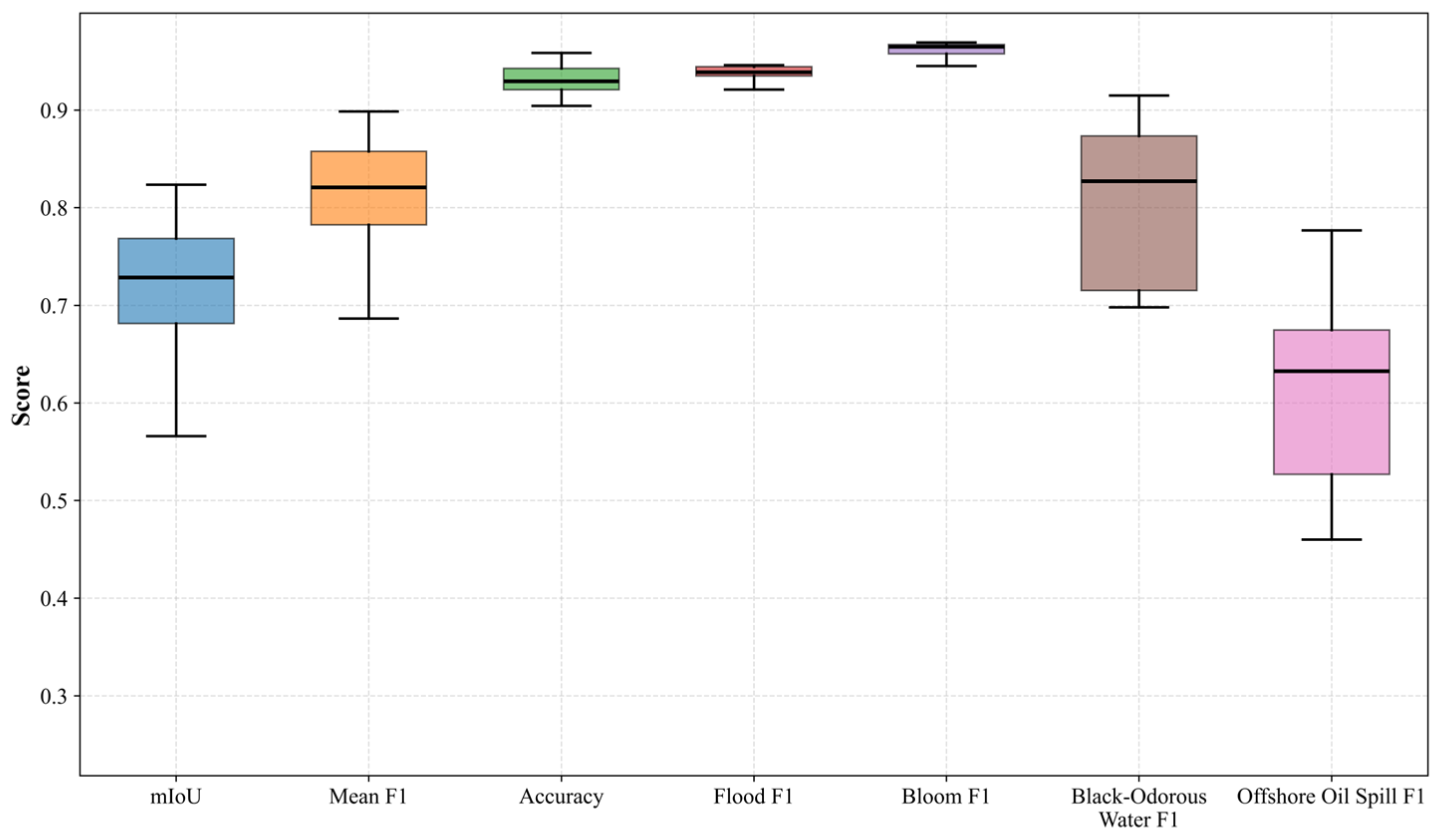
To evaluate the stability and robustness of the proposed model under different random seed initializations, we conducted 20 independent runs using distinct random seeds and performed statistical analyses on the results.

As Figure 5 illustrated, Accuracy, Flood F1, and Bloom F1 demonstrate compact distributions with median values exceeding 0.90, indicating a low sensitivity to random initialization. The comprehensive segmentation metrics, mIoU and Mean F1, achieve stable medians of approximately 0.73 and 0.82, respectively. However, varying degrees of variance are observed among the class-specific metrics. While the F1-scores for the Flood and Bloom classes show narrow interquartile ranges, the Black-Odorous Water F1 and Offshore Oil Spill F1 metrics exhibit higher dispersion. The F1-score for Black-Odorous Water ranges from approximately 0.70 to 0.91 with a median of 0.83. The Offshore Oil Spill F1 displays the highest variability, with values ranging between 0.46 and 0.78 and a median of 0.63. This variance suggests that the optimization process for offshore oil spills and black-odorous water bodies is more sensitive to initial weight configurations, which can be attributed to the spectral complexities and varying environmental conditions inherent to these specific target classes.

Overall, the model demonstrates relatively stable performance for Flood and Algal Bloom detection, while the Black-Odorous Water and Offshore Oil Spill categories exhibit larger performance fluctuations across different random seeds.

4. Discussion

4.1. Advantages of the Proposed Method

The effectiveness of the proposed method mainly arises from the explicit constraints imposed by the multisphere decision boundaries on feature distributions, which promote intra-class compactness and inter-class separation, thereby enhancing the overall discriminability among multiple water anomaly types. Specifically, each class is represented by a hypersphere characterized by a center and a radius, transforming the classification problem into a region-partitioning task. Under this formulation, each category corresponds to a bounded region in the feature space, and the class membership of a sample is determined by its distance to the corresponding class center and whether it falls within the associated region. Compared with conventional approaches that rely on implicit classification functions, this formulation provides a more explicit region-based description of class boundaries in the feature space.

To enforce such a structured feature distribution, a multisphere contrast loss (MSC Loss) is constructed as the optimization objective. The loss operates on Euclidean distances in the feature space, encouraging samples of the same category to move closer to their corresponding class centers while maintaining a certain distance from other class centers. Notably, the repel term is formulated based on the minimum distance between each sample and non-target class centers, such that only the closest competing class contributes to the loss. This mechanism emphasizes the most ambiguous class boundaries, instead of enforcing uniform separation from all non-target classes. Through this mechanism, the relative spatial relationships among samples directly participate in the optimization process, leading to a feature distribution that is more compact within classes and more separable across classes.

The multisphere decision boundaries and the MSC Loss are jointly optimized through an alternating strategy. When the feature mapping network is fixed, class centers and radii are updated based on the current feature representations, thereby defining the corresponding decision regions. Conversely, when the decision boundary parameters are fixed, the network parameters are optimized using the contrast loss to update the feature representations. Through this alternating process, region partitioning based on class centers and distance-based constraints are integrated into the feature learning process, progressively improving the separability of different categories in the feature space.

The impact of this mechanism is primarily reflected in the change in feature distribution rather than solely in classification accuracy. Visualization results based on principal component analysis (PCA) show that (Figure 3), in the original feature space, different anomaly types and normal surface samples exhibit noticeable overlap, particularly in boundary regions. After feature mapping, the distributions become more structured, with reduced overlap between categories and increased clustering around their respective centers. The relative spatial relationships between anomaly classes and normal surfaces become clearer, and the transition regions between categories are more distinct. In addition, the distance distributions indicate that samples tend to have smaller distances to their corresponding class centers and larger distances to the nearest non-target centers, which is consistent with the formulation of the multisphere decision boundaries. These results demonstrate that the proposed feature mapping mechanism effectively enhances class separability and stabilizes the decision boundary structure, thereby improving the robustness of multiclass anomaly discrimination.

Overall, the proposed method improves multiclass water anomaly discrimination by jointly leveraging a high-efficiency feature extraction module and explicitly structured multisphere decision boundaries with distance-based constraints. This design reduces feature overlap and enhances inter-class separability in the feature space, thereby enabling fast and accurate identification of water anomalies in complex remote sensing scenarios.

4.2. Limitations of the Proposed Method and Future Works

Although the proposed method markedly enhances multiclass anomaly recognition in water surface monitoring, several limitations should be noted. The model’s performance still depends on the representativeness and balance of the training data, and it tends to be less effective in identifying small-scale or rare anomaly types. Moreover, its generalizability across diverse environmental conditions and multi-sensor datasets has yet to be thoroughly assessed. In particular, future work will focus on extending the proposed method to integrate emerging Earth observation data sources, such as multi-sensor and multi-modal observations, with the aim of addressing data gaps under complex environmental conditions and improving its transferability across regions, sensors, and application scenarios.

5. Conclusions

This study proposes a deep multisphere decision boundaries (DMSDB) method for multiclass water anomaly detection. The core idea is to explicitly constrain feature distributions in the learned space by representing each anomaly category as a dedicated sphere defined by its center and radius, thereby transforming the classification problem into a structured region-partitioning task. By integrating multisphere decision boundaries with a contrastive optimization mechanism, the proposed method enhances intra-class compactness and inter-class separability, leading to more discriminative feature representations. To implement this method, a compact 5-dimensional feature space is first constructed based on remote sensing indices derived from Sentinel-2 imagery, and a modified VM-UNet-v2 network is employed to extract water anomaly response features (WARFs). Subsequently, a multi-sphere contrast loss function is introduced to optimize class-specific decision boundaries. Experimental results across four representative anomaly types—floods, algal blooms, black-odor water, and offshore oil spills—demonstrate that the proposed method achieves an average F1 score of 0.8789 and an mIoU of 0.7932. In addition, the model exhibits high inference efficiency, completing classification over a 10,000 km² scene within 33 s, indicating its suitability for large-scale rapid monitoring tasks. These results confirm that the performance improvement is closely related to the structured feature distributions guided by multisphere constraints, which effectively enhance the separability of spectrally similar anomaly categories. Nevertheless, several limitations remain. The effectiveness of the model still depends on the representativeness of the selected features and the scale of the training data, and its generalization capability under more diverse environmental and sensor conditions requires further investigation. Future work will focus on expanding the dataset, incorporating additional anomaly types, and validating the method under more complex scenarios. Overall, the proposed approach provides an effective and efficient solution for multiclass water anomaly detection by improving feature separability and applying efficient network architecture, offering a practical pathway for intelligent water environment monitoring.

References

1. Beyer, J.; Trannum, H.C.; Bakke, T.; Hodson, P.V.; Collier, T.K. Environmental Effects of the Deepwater Horizon Oil Spill: A Review. Mar. Pollut. Bull. 2016, 110, 28–51. [Google Scholar] [CrossRef] [PubMed]
2. Dudgeon, D.; Arthington, A.H.; Gessner, M.O.; Kawabata, Z.-I.; Knowler, D.J.; Lévêque, C.; Naiman, R.J.; Prieur-Richard, A.-H.; Soto, D.; Stiassny, M.L.J.; et al. Freshwater Biodiversity: Importance, Threats, Status and Conservation Challenges. Biol. Rev. 2006, 81, 163–182. [Google Scholar] [CrossRef] [PubMed]
3. Ahmed, S.F.; Kumar, P.S.; Kabir, M.; Zuhara, F.T.; Mehjabin, A.; Tasannum, N.; Hoang, A.T.; Kabir, Z.; Mofijur, M. Threats, Challenges and Sustainable Conservation Strategies for Freshwater Biodiversity. Environ. Res. 2022, 214, 113808. [Google Scholar] [CrossRef] [PubMed]
4. He, Y.; Leng, L.; Ji, X.; Wang, M.; Huo, Y.; Li, Z. Inversion and Analysis of Global Ocean Chlorophyll-a Concentration Based on Temperature Zoning. Remote Sens. 2024, 16, 2302. [Google Scholar] [CrossRef]
5. Jin, J.; Chen, F.; Yang, G.; Ye, Z.; Li, J.; Huang, T.; Huang, C. Delineating Bio-Optical Characteristics to Enhance Spatial-Based Quantification of CDOM in Clear to Turbid Waters. Int. J. Appl. Earth Obs. Geoinf. 2024, 132, 104033. [Google Scholar] [CrossRef]
6. Li, Z.; Chen, C.; Cao, N.; Jiang, Z.; Liu, C.; Adeyinka Oke, S.; Jim, C.; Zheng, K.; Zhang, F. High Spatial Resolution Inversion of Chromophoric Dissolved Organic Matter (CDOM) Concentrations in Ebinur Lake of Arid Xinjiang, China: Implications for Surface Water Quality Monitoring. Int. J. Appl. Earth Obs. Geoinf. 2024, 132, 104022. [Google Scholar] [CrossRef]
7. Yamamoto, K.; De Vries, T.; Siegel, D.A.; Nelson, N.B. Quantifying Biogeochemical Controls of Open Ocean CDOM from a Global Mechanistic Model. J. Geophys. Res. Oceans 2024, 129, e2023JC020691. [Google Scholar] [CrossRef]
8. Li, X.; Xiang, J.; Zhu, L.; Yang, Z.; Wei, T.; Mu, B.; Zhang, X.; Cui, T. Satellite-Observed Significant Improvement in Nearshore Transparency of the Bohai Sea during Pollution Control. Acta Oceanol. Sin. 2023, 42, 51–62. [Google Scholar] [CrossRef]
9. Alawadi, W.A.; Raheem, Z.A.H.A.; Yaseen, D.A. Use of Remote Sensing Techniques to Assess Water Storage Variations and Flood-Related Inflows for the Hawizeh Wetland. Environ. Monit. Assess. 2023, 195, 1246. [Google Scholar] [CrossRef] [PubMed]
10. Kislik, C.; Dronova, I.; Grantham, T.E.; Kelly, M. Mapping Algal Bloom Dynamics in Small Reservoirs Using Sentinel-2 Imagery in Google Earth Engine. Ecol. Indic. 2022, 140, 109041. [Google Scholar] [CrossRef]
11. Liu, M.; Li, T.; Liu, Y.; Li, J.; Jiang, H.; Wang, L.; An, S. Grading Identification and Pollution Source Determination of Rural Water Based on the Black-Odorous Water Quality Index Model. J. Water Process Eng. 2025, 75, 108076. [Google Scholar] [CrossRef]
12. Yang, Y.; Fan, X.; Zhou, C.; Wu, S.; Li, D.; Xu, G.; Li, G.; Ge, L. Urban Black and Odorous Water Body Mapping from Gaofen-2 Images. Open Geosci. 2022, 14, 1190–1205. [Google Scholar] [CrossRef]
13. Ren, Y.; Liu, Y. Surface Water Classification from GF-4 Images Using a Time Series Water Index. Int. J. Remote Sens. 2019, 40, 6336–6364. [Google Scholar] [CrossRef]
14. Markert, K.N.; Markert, A.M.; Mayer, T.; Nauman, C.; Haag, A.; Poortinga, A.; Bhandari, B.; Thwal, N.S.; Kunlamai, T.; Chishtie, F.; et al. Comparing Sentinel-1 Surface Water Mapping Algorithms and Radiometric Terrain Correction Processing in Southeast Asia Utilizing Google Earth Engine. Remote Sens. 2020, 12, 2469. [Google Scholar] [CrossRef]
15. Song, J.; Tian, J.; Zhu, L.; Zhou, B.; Qu, X.; Wang, C.; Luo, N.; Zhang, Z.; Guo, L.; Gao, M.; et al. Sub-Metre Surface Water Mapping Using Sentinel-1/2 with Integrated Super-Resolution and Deep Learning. Int. J. Remote Sens. 2025, 46, 9285–9307. [Google Scholar] [CrossRef]
16. Zhan, C.; Bai, K.; Tu, B.; Zhang, W. Offshore Oil Spill Detection Based on CNN, DBSCAN, and Hyperspectral Imaging. Sensors 2024, 24, 411. [Google Scholar] [CrossRef] [PubMed]
17. Hastie, T.; Tibshirani, R.; Friedman, J. The Elements of Statistical Learning; Springer Series in Statistics; Springer: New York, NY, USA, 2009; ISBN 978-0-387-84857-0. [Google Scholar]
18. Elsayed, G.F.; Krishnan, D.; Mobahi, H.; Regan, K.; Bengio, S. Large Margin Deep Networks for Classification 2018. In Proceedings of the 31st Advances in Neural Information Processing Systems (NeurIPS 2018), Montréal, QC, Canada, 2–8 December 2018. [Google Scholar]
19. Ghafoori, Z.; Leckie, C. Deep Multi-Sphere Support Vector Data Description. In Proceedings of the 2020 Siam International Conference on Data Mining (SDM); Demeniconi, C., Chawla, N., Eds.; Siam: Philadelphia, PA, USA, 2020; pp. 109–117. [Google Scholar]
20. Mishra, S.; Mishra, D.R. Normalized Difference Chlorophyll Index: A Novel Model for Remote Estimation of Chlorophyll-a Concentration in Turbid Productive Waters. Remote Sens. Environ. 2012, 117, 394–406. [Google Scholar] [CrossRef]
21. Lacaux, J.P.; Tourre, Y.M.; Vignolles, C.; Ndione, J.A.; Lafaye, M. Classification of Ponds from High-Spatial Resolution Remote Sensing: Application to Rift Valley Fever Epidemics in Senegal. Remote Sens. Environ. 2007, 106, 66–74. [Google Scholar] [CrossRef]
22. Xu, H. Modification of Normalised Difference Water Index (NDWI) to Enhance Open Water Features in Remotely Sensed Imagery. Int. J. Remote Sens. 2006, 27, 3025–3033. [Google Scholar] [CrossRef]
23. Yao, Y.; Shen, Q.; Zhu, L.; Gao, H.J.; Cao, H.Y.; Han, H.; Sun, J.G.; Li, J.S. Remote sensing identification of urban black-odor water bodies in Shenyang city based on GF-2 image. J. Remote Sens. 2019, 23, 230–242. [Google Scholar] [CrossRef]
24. Rajendran, S.; Sadooni, F.N.; Al-Kuwari, H.A.-S.; Oleg, A.; Govil, H.; Nasir, S.; Vethamony, P. Monitoring Oil Spill in Norilsk, Russia Using Satellite Data. Sci. Rep. 2021, 11, 3817. [Google Scholar] [CrossRef] [PubMed]
25. Zhang, M.; Yu, Y.; Gu, L.; Lin, T.; Tao, X. VM-UNET-V2 Rethinking Vision Mamba UNet for Medical Image Segmentation 2024. In Proceedings of the Bioinformatics Research and Applications: 20th International Symposium, ISBRA 2024, Kunming, China, 19–21 July 2024. [Google Scholar]
26. Peng, Y.; Chen, D.Z.; Sonka, M. U-Net V2: Rethinking the Skip Connections of U-Net for Medical Image Segmentation. In Proceedings of the 2025 IEEE 22nd International Symposium on Biomedical Imaging (ISBI), Houston, TX, USA, 14–17 April 2025; pp. 1–5. [Google Scholar]
27. Howard, A.G.; Zhu, M.; Chen, B.; Kalenichenko, D.; Wang, W.; Weyand, T.; Andreetto, M.; Adam, H. MobileNets: Efficient Convolutional Neural Networks for Mobile Vision Applications. arXiv 2017, arXiv:1704.04861. [Google Scholar]
28. Woo, S.; Woo, S.; Park, J.; Park, J.; Lee, J.-Y.; Lee, J.-Y.; Kweon, I.S.; Kweon, I.S. CBAM: Convolutional Block Attention Module. In Proceedings of the Computer Vision—ECCV 2018; Springer: Munich, Germany, 2018; pp. 3–19. [Google Scholar] [CrossRef]
29. Huber, P.J. Robust Estimation of a Location Parameter. In Breakthroughs in Statistics; Springer: New York, NY, USA, 1992; pp. 492–518. [Google Scholar] [CrossRef]
Figure 1. Overview of the DMSDB method: (a) Acquisition of Sentinel-2 remote sensing imagery; (b) Extraction of multidimensional spectral features; (c) Construction of multi-sphere decision boundaries; (d) Intelligent remote sensing detection of water anomalies.
Remotesensing 18 02273 g001
Figure 2. Geographic locations of the selected water surface anomaly cases.
Remotesensing 18 02273 g002
Figure 3. Visualization of feature space transformation for water anomaly discrimination: (a) Original Remote Sensing Feature Space, (b) Neural Network Feature Mapper, (c) Enhanced Feature Space.
Remotesensing 18 02273 g003
Figure 4. Natural-color images of water anomaly events, along with their corresponding detection results and ground truth data. From left to right: the natural-color image of the anomaly event; detection results obtained using three different decision boundary strategies (ν = 0.1, ν = 0.05, ν = 0.01); and the ground truth annotation for each event. The color-coded legend identifies the five thematic categories used in the detection results: normal area (0), flood (1), algal bloom (2), black-odor water (3), and offshore oil spill (4).
Remotesensing 18 02273 g004
Figure 5. Random Seed Overall Distribution.
Remotesensing 18 02273 g005