Estimation of High-Resolution Multi-Layer Soil Moisture Using Land Data Assimilation and the Three-Cornered Hat Method

Highlights

What are the main findings?

• An HRSM dataset was generated by fusing multi-source satellite observations (SMAP, HJ-2, Sentinel-2, and Gaofen-6) using the ESTARFM model.
• Within the EnKF framework, the TCH method effectively characterizes observation errors in HRSM and improves the accuracy of both surface and root-zone SM estimates.

What are the implications of the main findings?

• The DA_HRSM framework provides higher-resolution spatial representations of SM and captures spatial heterogeneity across irrigation districts, offering improved land surface information for regional water resource management.
• The DA_HRSM estimates successfully capture the spring drought event in central Yunnan, China, demonstrating the practical utility of the framework for drought monitoring and agricultural applications.

Abstract

Soil moisture (SM) plays a pivotal role in regulating terrestrial energy-water exchanges and exerts substantial influence on agricultural productivity. In this study, a high-resolution soil moisture (HRSM) dataset (16 m) was generated by integrating multi-source remote sensing data from SMAP, HJ-2, Sentinel-2, and Gaofen-6, together with the Enhanced Spatial and Temporal Adaptive Reflectance Fusion Model. The data assimilation (DA) method was implemented for assimilating HRSM within the Ensemble Kalman Filter (EnKF) framework using the Noah-MP model at a spatial resolution of 1 km. To enhance the spatial detail of SM, HRSM and its relative uncertainties derived from the three-cornered hat (TCH) method were used to update the observation error and Kalman gain in the EnKF framework, thereby improving SM profile estimates at a 16 m resolution. The performance of the DA method was evaluated against in situ measurements during the spring drought period in central Yunnan Province, China. The results show that assimilating HRSM (DA_HRSM) significantly improves surface and root-zone SM estimates in the Noah-MP model. The simulated SM from the DA_HRSM method demonstrates lower relative uncertainty. Compared to the assimilation of SMAP SM, the DA_HRSM method provides higher-resolution spatial features of SM and enhances spatial heterogeneity across 20 irrigation districts. The DA_HRSM method effectively captured the spring drought in central Yunnan, demonstrating good agreement with the Palmer Drought Severity Index (PDSI). The result highlights the advantages of incorporating high-resolution SM data into agricultural and drought monitoring systems.

1. Introduction

Soil moisture (SM) plays an essential role in regulating the terrestrial water cycle across regional and global scales [1]. It influences the hydrological cycle and regulates water distribution and ecosystem accessibility. Surface soil moisture (SSM) serves as a key factor driving environmental variability and influencing terrestrial processes and climate simulations [2]. Root-zone soil moisture (RZSM) controls the absorption of water and nutrients by the plant roots and affects plant growth [3]. Therefore, an accurate representation of SM spatial patterns, especially through high-resolution SSM and RZSM simulations, is crucial for drought monitoring, weather forecasting, and agricultural yield estimation [4,5].

Currently, methods for estimating SM can be categorized into three major types: in situ observations, satellite remote sensing, and physics-based models [6]. Traditionally, ground-based observations have been utilized to obtain accurate estimates of SM profiles. However, due to the sparse spatial distribution of station observations, it is challenging to accurately characterize large-scale SM patterns, particularly in regions with significant spatial heterogeneity [7]. In contrast, satellite remote sensing enables rapid retrieval of SSM (0–5 cm) through measurements of terrestrial microwave emissions and backscatter signals from passive and active sensors [1]. Several satellite missions have been developed for SSM monitoring, including: (1) the Advanced Scatterometer (ASCAT) employing C-band radar technology [8]; (2) the Soil Moisture and Ocean Salinity (SMOS) mission utilizing L-band passive microwave synthetic aperture radiometer (MIRAS) [9]; (3) the Advanced Microwave Scanning Radiometer 2 (AMSR2) with multi-frequency passive microwave sensors [10]; (4) the Soil Moisture Active Passive (SMAP) mission providing L-band passive microwave radiometer observations [11].

Beyond these satellite missions, the Cyclone Global Navigation Satellite System (CYGNSS), which employs GNSS-Reflectometry (GNSS-R) technology, has demonstrated considerable potential for SM retrieval [12]. As a form of opportunistic L-band microwave sensing that exploits reflected GNSS signals, CYGNSS provides high-revisit observations and relatively finer effective spatial sampling, making it a promising complementary data source for SM estimation. Recent studies have successfully employed a variety of machine learning and deep learning approaches, ranging from random forest algorithms to vision Transformer (ViT)-based models, for SM retrieval using CYGNSS observations [13,14]. However, passive microwave remote sensing observations are generally limited to SSM retrieval and suffer from coarse spatial resolutions. Consequently, these data generally cannot meet the requirements for agricultural monitoring at the field scale.

Land surface models (LSMs) are widely applied to simulate key terrestrial processes, such as SM dynamics, vegetation growth, and exchanges between the land and atmosphere [15]. Among various LSMs, the Noah-MP (Noah land surface model with multi-parameterization options) model has been widely used for hydrological modeling and to generate spatio-temporally continuous SM estimates [16]. However, accurately simulating SM remains a significant challenge due to simplified physical structures, insufficient parameterization, and uncertainties in input data [17,18]. LSMs parameterized with irrigation schemes are an effective approach for simulating SM in agricultural regions [19]. However, accurately representing anthropogenic irrigation processes in these models remains challenging, with the uncertainty of SM simulations being particularly pronounced at the regional scale.

Data assimilation (DA) methods are proposed to provide an explicit framework for addressing uncertainties in model inputs, parameters, and structure, as well as for integrating observations with model simulations [11,20,21]. Recent research has aimed to alleviate model uncertainties in LSMs and improve simulation accuracy through assimilation of SM, leaf area index (LAI), and terrestrial water storage [11,22,23]. Zhao et al. [24] found that assimilating AMSR-E brightness temperature into the CLM4 model improves multi-layer SM estimates at the global scale. Seo et al. [11] demonstrated that assimilating SMAP and ASCAT SM into the JULES model improves the simulation accuracy of RZSM. Moreover, Ahmad et al. [25] suggested that SMAP assimilation provides additional improvement compared to SM simulations using Noah-MP. By using the hybrid DA and machine learning methods, He et al. [26,27] demonstrated that integrating remote sensing and ground-based observations into the Noah-MP model improves the estimation of SM in semi-arid regions.

Based on the aforementioned research, DA methods have been widely applied to the assimilation of SM from SMAP, AMSR-E, and ASCAT. However, SM simulations in LSMs are limited by the coarse spatial resolution of microwave observations, which fail to capture the fine-scale SM variations. High-resolution optical and thermal infrared data can effectively capture fine-scale irrigation signals and soil-vegetation heterogeneity in agricultural landscapes. However, this information is not yet fully integrated into current DA frameworks. In addition, the computational cost of DA methods increases exponentially with higher spatial resolution, especially in land surface modeling. Consequently, the direct integration of high-resolution soil moisture (HRSM) observations and their error characteristics into land surface modeling remains a significant challenge.

To overcome these challenges, this study presents a DA framework that integrates the Ensemble Kalman Filter (EnKF) and three-cornered hat (TCH) methods to generate high-resolution, multi-layer SM estimates. The TCH method was used to update observation errors and the Kalman gain in the DA framework. Based on the proposed DA framework, this study aims to: (1) generate HRSM using the SMAP, HJ-2, Sentinel-2, and Gaofen-6 data; (2) assimilate HRSM into the Noah-MP model to improve the multi-layer SM estimates; (3) compare results with open-loop (OL) and SMAP SM assimilation and conduct uncertainty assessment using the TCH method; and (4) evaluate the benefits of high-resolution DA for irrigation district simulations and regional drought monitoring.

2. Study Area and Data

2.1. Study Area

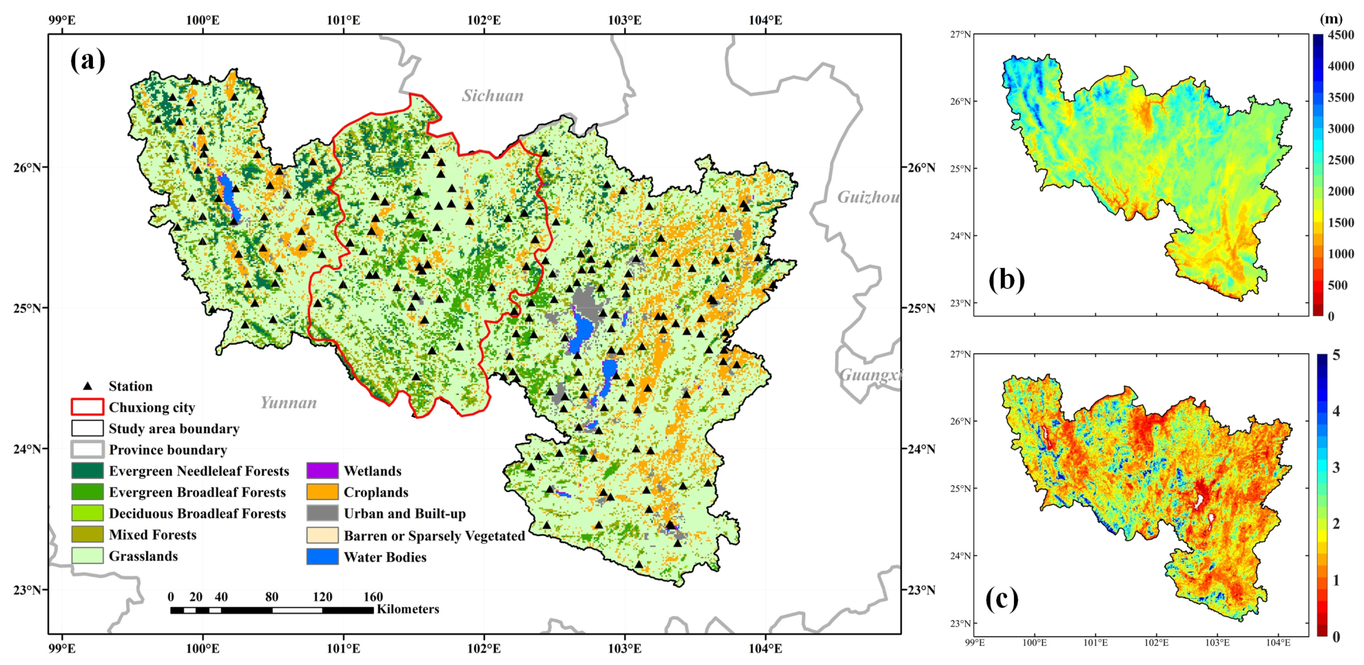
The study region is located in central Yunnan Province, China, covering a total area of approximately 106,144 km² (Figure 1a). The landforms in central Yunnan Province are diverse, including plains, plateaus, and hills (Figure 1b). Influenced by a distinct subtropical monsoon climate, the region experiences an average annual rainfall of 830 mm, with nearly 70% of the total precipitation concentrated in the summer (June to August), while the winter months remain markedly dry (December to February). The vegetation composition in the region is notably diverse, comprising grasslands (64.96%), forests (20.71%), and croplands (11.15%). In recent years, Yunnan Province has experienced increasingly severe drought conditions, with particularly pronounced impacts during the spring season (February–April). The worsening drought has led to substantial social and economic losses across the region [28]. Beyond these immediate impacts, the persistent drought has also disrupted vegetation carbon sequestration processes, making the region a critical hotspot of national and global environmental concern [29]. This study selected the period from January to June 2024 to evaluate the performance of assimilating HRSM during the severe drought period.

2.2. Dataset

2.2.1. Meteorological Data

In this study, the China Meteorological Forcing Dataset (CMFD) was used as the meteorological forcing dataset to drive the Noah-MP land surface model. It integrates multiple data sources, including in situ observations from the China Meteorological Administration, remote sensing products, and reanalysis datasets such as European Centre for Medium-Range Weather Forecasts ERA5, through advanced data fusion and bias-correction techniques [30]. CMFD provides near-surface meteorological variables at a spatial resolution of 0.1° and a temporal resolution of 3 h, covering the period from 1951 to 2024 (https://data.tpdc.ac.cn/zh-hans/data/) (accessed on 6 December 2024).

2.2.2. Remote Sensing Data

In the DA method, the SM data were obtained from the HRSM dataset for central Yunnan. The data sources include daily SMAP SM at 9 km resolution, SMAP/Sentinel-1 SM at 1 km resolution, and multispectral data from HJ-2 (16 m), Sentinel-2 (10 m), and Gaofen-6 (16 m).

The SMAP mission provides global measurements of SM to support hydrological, agricultural, and climate-related studies. The SPL3SMP_E (Level 3 Passive Soil Moisture) product was derived from SMAP passive L-band radiometer data and offers global daily SSM estimates at a 9 km resolution (https://nsidc.org/data/smap/) (accessed on 10 October 2024). The SMAP/Sentinel-1 enhanced SM product is a high-resolution dataset generated by synergistically combining L-band brightness temperatures from the SMAP mission (both ascending and descending) with C-band backscatter data from the Sentinel-1 satellite (https://search.earthdata.nasa.gov/) (accessed on 10 October 2024). This Level 2 product (SPL2SMAP_S) provides SM estimates at a 1 km spatial resolution. The retrievals were derived from downscaled brightness temperature using a linear relationship between microwave brightness temperature and synthetic aperture radar (SAR) backscatter under specified vegetation cover and surface conditions. Due to the orbital configuration and acquisition schedule of Sentinel-1 observations, the SMAP/Sentinel-1 SM product was typically acquired at approximately 11-day intervals over the study area [31].

The HJ-2 (Huanjing-2) satellite constellation, comprising HJ-2A and HJ-2B, is part of an environmental monitoring program in China. Equipped with multispectral sensors covering 16 spectral bands from visible to infrared, it offers spatial resolutions of 16 m to 100 m (http://www.cresda.cn) (accessed on 10 October 2024). With a combined swath of 300 km and a 4-day revisit cycle, HJ-2 enables effective monitoring of ecological changes, environmental quality, and natural disasters. Sentinel-2, operated by the European Space Agency under the Copernicus Programme, is a dual-satellite system composed of Sentinel-2A and Sentinel-2B. Both satellites are equipped with multispectral sensors providing 13-band high-resolution imagery covering the visible to shortwave infrared spectrum. With spatial resolutions of 10, 20, and 60 m and a swath width of 290 km, the mission enables detailed observation of Earth’s surface and offers a 5-day revisit interval (https://dataspace.copernicus.eu/) (accessed on 10 October 2024). Gaofen-6 (GF-6) is part of the High-resolution Earth Observation System in China, launched to provide frequent and high-resolution optical imagery for agricultural and environmental applications. The satellite offers optical imagery at a 2 m resolution in the panchromatic band and 16 m resolution in the multispectral bands, with a revisit cycle of approximately 4 days (https://data.cresda.cn/) (accessed on 13 October 2024).

LAI data were obtained from the MODIS dataset, with a spatial resolution of 500 m and an 8-day temporal frequency (https://search.earthdata.nasa.gov/) (accessed on 10 October 2024). In the Noah-MP model, land cover types were updated using MODIS products (https://lpdaac.usgs.gov/) (accessed on 10 October 2024) to enable more robust characterization of land surface conditions. LAI and land cover type data were resampled to a 1 km resolution to match the Noah-MP model. Additionally, 1 m resolution land cover data from Li et al. [32] were used in the SM fusion algorithm to provide high-resolution land surface features. To further evaluate the assimilation results, the ERA5-Land reanalysis data were used for comparison with the simulated SM. Based on the HTESSEL land surface model, the ERA5-Land dataset provides SM across four layers (0–289 cm), with a spatial resolution of approximately 9 km and an hourly temporal resolution. The Palmer Drought Severity Index (PDSI), an established metric for SM drought, was employed to independently validate the drought characteristics in central Yunnan. The PDSI algorithm models soil water balance based on fundamental climatic parameters. This study used PDSI data from the TerraClimate dataset (https://climatedataguide.ucar.edu/) (accessed on 10 October 2024). More details regarding the multi-source remote sensing data are presented in

Table 1. The multi-source remote sensing datasets employed in this study.

Variables	Sensor/Mission	Spatial Resolution	Temporal Resolution
SM	SMAP	9 km	Daily
SM	SMAP/Sentinel-1	1 km	11 days
Multi-spectral data	HJ-2	16 m	4 days
Multi-spectral data	Sentinel-2	10 m	5 days
Multi-spectral data	Gaofen-6	16 m	4 days
LAI	MODIS	500 m	8 days
Land cover types	MODIS	500 m	-
Land cover types	SinoLC-1	1 m	-
PDSI	TerraClimate	4 km	monthly

.

2.2.3. In Situ SM Measurements

For model development and evaluation, in situ SM measurements provided by the Department of Water Resources of Yunnan Province were employed. The network provides hourly observations at depths of 10, 20, and 40 cm. In this study, the 10 and 40 cm measurements were selected to represent SSM and RZSM, respectively, consistent with the corresponding soil layers in the Noah-MP model. Additionally, we removed data that fell outside the physical range and excluded observations taken during soil freezing. Daily SM was calculated by averaging the hourly data after quality control. A total of 176 observation stations were distributed across central Yunnan, with 40 located in Chuxiong City. These stations cover the dominant land cover types in central Yunnan, including grassland (103 sites), cropland (59 sites), forest (8 sites), and urban/built-up areas (6 sites), thereby providing a representative sampling of SM variability and supporting model development across the study area.

3. Methodology

This study presents a DA framework that assimilates HRSM into the Noah-MP model using the EnKF method. Observation errors were estimated using the TCH method to generate high-resolution SSM and RZSM (16 m) estimates. To start, remote sensing data from SMAP, HJ-2, Sentinel-2, and Gaofen-6 were used to generate HRSM (16 m). Next, HRSM and LAI data were assimilated into the Noah-MP model to improve the accuracy of SM estimates at a 1 km resolution. Within this framework, the TCH method was employed to quantify the relative uncertainties in the HRSM data, which were subsequently utilized to update the observation error and Kalman gain (16 m) in the DA system. Finally, HRSM data were integrated to update the model states and generate high-resolution and temporally continuous SM at a 16 m resolution.

3.1. Noah-MP Model

The Noah-MP model is an advanced version of the original Noah LSM. It incorporates multiple parameterization schemes for key processes such as SM, vegetation dynamics, snow accumulation and melt, and energy fluxes [33,34]. This enables greater flexibility and improved accuracy in simulating land surface processes under various environmental conditions. The Noah-MP model relies on a range of meteorological data to accurately simulate land surface processes. The model also requires detailed land surface characteristics, including land cover types, vegetation parameters, soil properties, and topographical features. Initial conditions for soil moisture, temperature profiles, and snowpack conditions are essential for starting simulations. The estimation of soil temperature and moisture consists of four vertical soil layers with depths of 0.1 m, 0.4 m, 1.0 m, and 2.0 m, respectively [35]. This study employed the Noah-MP model, configured with the modified two-stream radiative transfer scheme, the Noah β-factor scheme, Monin–Obukhov turbulence scheme, and TOPMODEL with groundwater scheme for SM simulation.

3.2. The Estimation of HRSM

To generate 16 m HRSM data, the following steps were implemented:

In the first step, the SMAP 9 km SM was resampled to a 1 km resolution. The overpass dates of the SMAP/Sentinel-1 1 km product were selected and matched with corresponding SMAP 9 km data to construct the input dataset. The Enhanced Spatial and Temporal Adaptive Reflectance Fusion Model (ESTARFM) was employed to establish the relationship between SMAP and SMAP/Sentinel-1 SM. Specifically, ESTARFM utilized paired SMAP (9 km) and SMAP/Sentinel-1 (1 km) observations to establish spatiotemporal relationships, which were then used to generate 1 km SM estimates on dates when only SMAP data were available. In this study, 16 pairs of coarse- and fine-resolution reference images were used in this process.

ESTARFM is a widely used data fusion algorithm designed to generate high spatio-temporal resolution imagery by combining coarse- and fine-resolution remote sensing data. It assumes that temporal changes within homogeneous land cover types are spatially consistent and can be transferred from fine-resolution images to coarse-resolution observations. By leveraging this spatio-temporal relationship, ESTARFM can effectively reconstruct missing fine-resolution information between acquisition dates [36,37]. Compared with regression-based downscaling methods, ESTARFM provides a more physically consistent spatio-temporal fusion framework and does not rely on strong linearity assumptions, making it more suitable for landscapes with strong spatial heterogeneity.

In the second step, the Soil Water Index (SWI) proposed by Wang et al. [35] was applied to capture high-resolution SM characteristics using data from the HJ-2, Sentinel-2, and GF-6 satellites. This study uses the SWI by strategically combining red-edge bands (e.g., REB1 and REB2) with traditional spectral bands such as red and near-infrared (NIR). The SWI was calculated as follows:

$$\mathrm{S}\mathrm{W}\mathrm{I}=({\rho }_{red}+M{\rho }_{REB2}-f_v({\rho }_{vREB1}+M{\rho }_{vREB2}))/((1-f_v)\sqrt{1+M^2})$$

(1)

where M represents the slope of the soil line composed of the corresponding bands. ρ_red and ρ_REB2 denote the reflectance of the red and red-edge 2 bands, respectively. ρ_vREB1 and ρ_vREB2 represent the reflectance of REB1 and REB2 at pixels corresponding to maximum vegetation coverage in each image. f_v denotes fractional vegetation cover and can be expressed as

$$f_v=1-{(({NDVI}_{max}-NDVI)/({NDVI}_{max}-{NDVI}_{min}))}^{0.6175}$$

(2)

NDVI is the Normalized Difference Vegetation Index, which was calculated from red and NIR reflectance.

A linear regression model was constructed between the SWI and in situ SM measurements. In this model, the ordinary least squares method was applied to identify the optimal spectral bands and parameters. Since model performance is closely related to the input samples, this study selected 136 SM stations across central Yunnan (excluding Chuxiong City) for model construction. The constructed regression model (SM = 0.537 × SWI + 0.023) was used to estimate regional 16 m SM. By leveraging the enhanced spectral sensitivity of the red-edge bands in GF-6 and Sentinel-2 to vegetation water content, this method demonstrates significant advantages over traditional vegetation index-based approaches, particularly for precision agriculture in irrigation-intensive areas [38]. The 16 m SM product was generated to align with the spatial resolution of the HJ-2 and Gaofen-6 datasets. This high-resolution objective is intended to maximize the use of fine-scale spatial information from optical remote sensing observations.

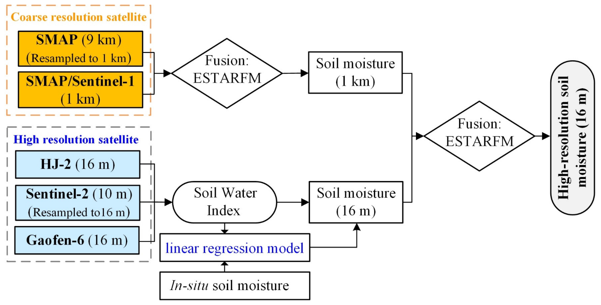
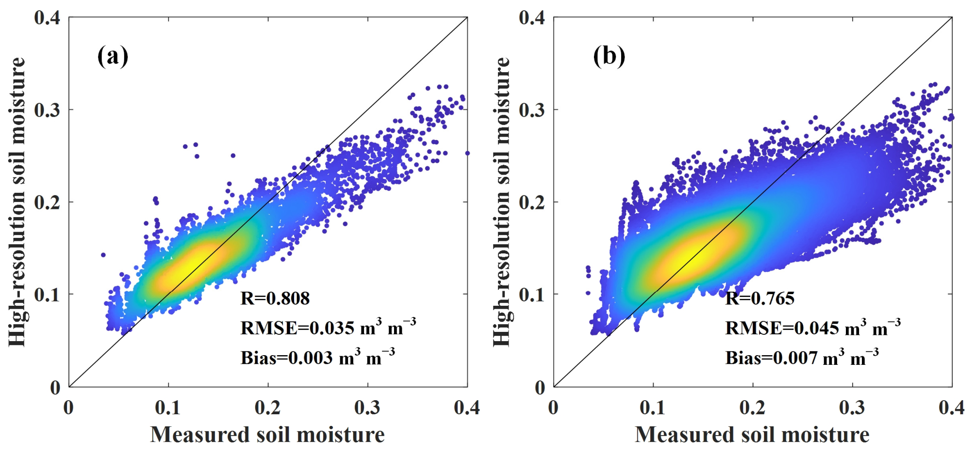
Finally, the generated daily 1 km SM from the first step and the 16 m SM from the second step were uniformly resampled to a 16 m resolution. The 16 m land cover data (resampled from 1 m) were incorporated into the ESTARFM model to constrain the similar-pixel search range within homogeneous land cover types, thereby reducing interference from heterogeneous surfaces. The ESTARFM model was then applied to generate the final 16 m HRSM product. The estimation process for HRSM is illustrated in Figure 2. The scatter plots of in situ validation for the HRSM dataset are shown in Appendix A, Figure A1. The results indicate a high consistency between the HRSM estimates and the in situ observations, with values closely aligned along the 1:1 line. The RMSE values for Chuxiong City and central Yunnan Province are 0.035 and 0.045 m³ m⁻³, respectively.

3.3. Data Assimilation Using EnKF

The EnKF is a sequential DA approach that adjusts model states and parameters by generating ensembles and updating predictions based on the covariance between state variables and observations [39]. In this study, the EnKF method was used to assimilate remotely sensed LAI and HRSM into the Noah-MP model to improve the estimation accuracy of vegetation dynamics and four-layer SM.

In the forecast step, the Noah-MP model was run at 1 km spatial resolution to reduce computational costs. The leaf biomass and four-layer SM were perturbed within the ensemble to generate model forecast error covariance. In the update step, 1 km MODIS LAI were perturbed to represent the observation error covariance. Based on this, the model state variable (leaf biomass) was updated using MODIS LAI and the Kalman gain (Equation (4)), which was calculated from the forecast and observation error covariance. In this study, LAI was assimilated into the Noah-MP model to improve the accuracy of vegetation dynamics.

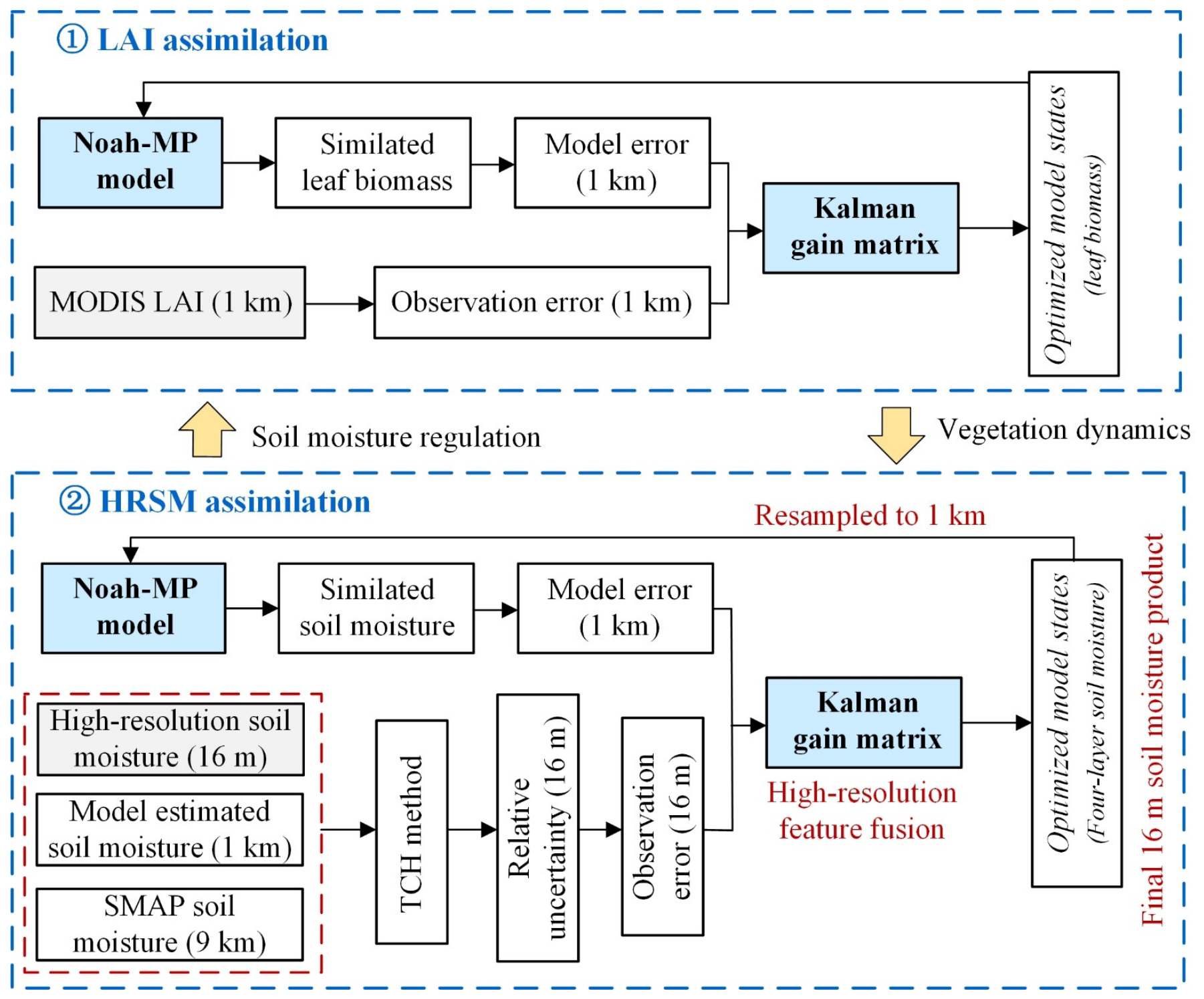
For HRSM assimilation (DA_HRSM), this study employed the cumulative distribution function (CDF) to minimize bias between satellite-retrieved SM and model simulations by matching observational and model data. The TCH method was employed to quantify the high-resolution relative uncertainties of HRSM, capturing the spatial patterns of observational errors. The HRSM (16 m), model-simulated SM (1 km), and SMAP SM (9 km) were used to compute the observation error of HRSM. In addition, the HRSM and its associated observation error were used to compute the Kalman gain, which was then applied to update the model and generate four-layer SM simulations at a 16 m resolution. Finally, the updated 16 m SM simulations were resampled to a 1 km resolution for use in the subsequent assimilation cycle. Overall, the DA system was implemented at a 1 km spatial resolution, while SM updates were performed at a 16 m resolution. This design represents a trade-off between computational feasibility and spatial detail, as running the DA system at the native 16 m resolution would substantially increase computational costs and memory demands, making long-term simulations over the study domain computationally prohibitive. The DA workflow is summarized in Figure 3. During the assimilation process, a white noise of 10 g m⁻² was incorporated into leaf biomass [22]. The standard deviations for the four-layer SM were set to 0.03, 0.03, 0.025, and 0.02 m³ m⁻³, respectively [40]. Additionally, a standard deviation of 0.1 (−) was applied to the remotely sensed LAI [22]. An ensemble size of 30 members was adopted in the DA system to ensure stable assimilation performance while maintaining reasonable computational efficiency [41,42].

The key equation of the EnKF method was given by

$$x_i^a=x_i^f+\mathit{K}(y-H(x_i^f))$$

(3)

where $x_i^a$ and $x_i^f$ are the analyzed and forecasted state vectors (leaf biomass and four-layer SM). y is the observation variable (LAI and HRSM). H is the observation operator that maps the model state to observation space and K is the Kalman gain matrix.

The Kalman gain was calculated as

$$\mathit{K}=P{H}^T{(HP{H}^T+R)}^{-1}$$

(4)

where P and R denote the error covariance matrices associated with the forecast and observations, respectively. The EnKF weights the model predictions and observational data based on the uncertainties captured by the Kalman gain, thereby obtaining optimized leaf biomass and four-layer SM estimates.

The Noah-MP model was spun up for 24 years (2000–2023) to reach equilibrium in SM and other state variables. The simulations of the DA method were conducted for six months (1 January to 30 June, i.e., DOY 1-181), covering parts of winter, spring, and early summer in 2024. Daily LAI and HRSM values were assimilated into the Noah-MP model (hereafter referred to as DA_HRSM) at 00:00 local time to update leaf biomass and initialize SM. For comparison, remotely sensed LAI and SMAP SM were directly assimilated into the Noah-MP model using the EnKF approach (DA_SMAP). In both the DA_HRSM and DA_SMAP methods, remotely sensed LAI data at the same spatial resolution (1 km) were assimilated to compare the effects of SM data at different resolutions on the simulation results.

3.4. Uncertainty Estimation Using the TCH Method

The TCH method is a statistical technique for evaluating the relative uncertainties of different datasets without requiring a priori information [43,44]. In the TCH algorithm, n different datasets are represented by ${\left\{X_i\right\}}_{i=1,2,\dots ,n}$, where X_i denotes the i-th dataset. The TCH represents each dataset as

$$X_i=X_t+{\sigma }_i,\forall i=1,2,\dots ,n$$

(5)

where X_t is defined as the true value among the n different SM datasets and σ_i represents the zero-mean error of the i-th dataset. The difference between the remaining (n − 1) datasets and the true value is expressed as

$$y_i=X_i-X_r={\sigma }_i-{\sigma }_r,i=1,2,\dots ,n-1$$

(6)

In this equation, X_r is arbitrarily selected from the SM datasets and y_i is a matrix containing the n − 1 difference sequences. The difference sequences are stored in the Y matrix as follows:

$$\mathbf{Y}=\left[\begin{array}{cccc}{y}_{11}& y_{12}& \cdots & y_{1(\mathrm{n}-1)}\\ y_{21}& y_{22}& \cdots & y_{2(\mathrm{n}-1)}\\ ⋮& ⋮& ⋮& ⋮\\ y_{\mathrm{m}1}& y_{\mathrm{m}2}& \cdots & y_{\mathrm{m}(\mathrm{n}-1)}\end{array}\right]$$

(7)

where m represents the length of each dataset. The covariance matrix corresponding to these difference sequences is

$$\mathbf{C}=\mathrm{cov}(\mathbf{Y})=\left[\begin{array}{cccc}{c}_{11}& c_{12}& \cdots & c_{1(\mathrm{n}-1)}\\ c_{21}& c_{22}& \cdots & c_{2(\mathrm{n}-1)}\\ ⋮& ⋮& ⋮& ⋮\\ c_{\mathrm{m}1}& c_{\mathrm{m}2}& \cdots & c_{\mathrm{m}(\mathrm{n}-1)}\end{array}\right]$$

(8)

Here, cov (Y) is the covariance calculation equation. When i = j, c_ij represents the uncertainty of different datasets, and when I ≠ j, c_ij represents the covariance estimate. Galindo & Palacio [45] introduced a noise covariance symmetric matrix R, constructing the following relationship:

$$\mathbf{C}=\mathbf{B}\cdot \mathbf{R}\cdot {\mathbf{B}}^{\mathrm{T}}$$

(9)

The matrix B can be expressed as

$${\mathbf{B}}_{n-1,n}=\left[\begin{array}{ccccc}1& 0& \cdots & 0& -1\\ 0& 1& \cdots & 0& -1\\ ⋮& ⋮& ⋮& ⋮& ⋮\\ 0& 0& 0& \cdots & -1\end{array}\right]$$

(10)

The matrix R can be expressed as

$$\mathbf{R}=\left[\begin{array}{cccc}{r}_{11}& r_{12}& \cdots & r_{1\mathrm{n}}\\ r_{21}& r_{22}& \cdots & r_{2\mathrm{n}}\\ ⋮& ⋮& ⋮& ⋮\\ r_{1\mathrm{n}}& r_{2\mathrm{n}}& \cdots & r_{\mathrm{nn}}\end{array}\right]$$

(11)

Finally, the solution for the matrix R can be obtained using the Kuhn–Tucker theory [45]. The final uncertainty of the data can be calculated by taking the square root of the diagonal elements of the R matrix and dividing this by the mean of each SM product.

3.5. Evaluation Metrics

The root mean square error (RMSE) and correlation coefficient (R) were used to evaluate the results of the DA system. To assess the spatial variability of SM in the irrigation districts, the coefficient of variation (CV) was calculated as follows:

$$\mathrm{CV}=\frac{\sigma }{\mu }=\frac{\sqrt{\frac{1}{n}{\displaystyle \sum _{i=1}^n}{(x_i-\overline{x})}^2}}{\overline{x}}$$

(12)

where σ represents the standard deviation of the SM, x is the mean value of the data, and n represents the number of data samples.

This study evaluates the performance of high-resolution DA for drought monitoring based on the Soil Moisture Condition Index (SMCI). The calculation equation is as follows:

$$\mathrm{S}\mathrm{M}\mathrm{C}\mathrm{I}=\frac{\mathrm{S}\mathrm{M}-{\mathrm{S}\mathrm{M}}_{\min }}{{\mathrm{S}\mathrm{M}}_{\max }-{\mathrm{S}\mathrm{M}}_{\min }}$$

(13)

SM represents the weekly average SM, while SM_min and SM_max denote the minimum and maximum SM values, respectively. Here, SM_min and SM_max were calculated from the weekly average results of SMAP SM for each grid from 2015 to 2024. This index was calculated based on weekly averages, allowing it to capture the characteristics of short-term droughts and exclude the effects of seasonal variations. The index ranged from 0 to 1, with lower values indicating more severe drought [46].

4. Results

4.1. Performance of the DA_HRSM Method

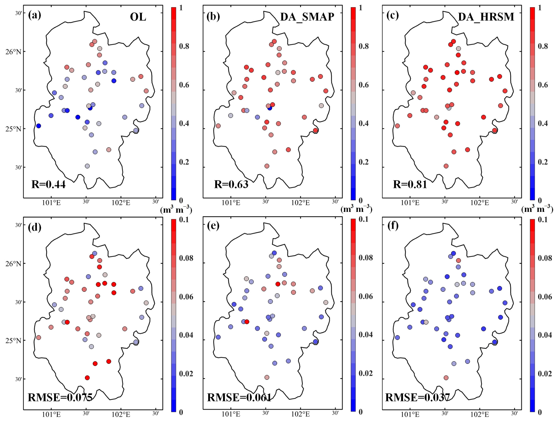
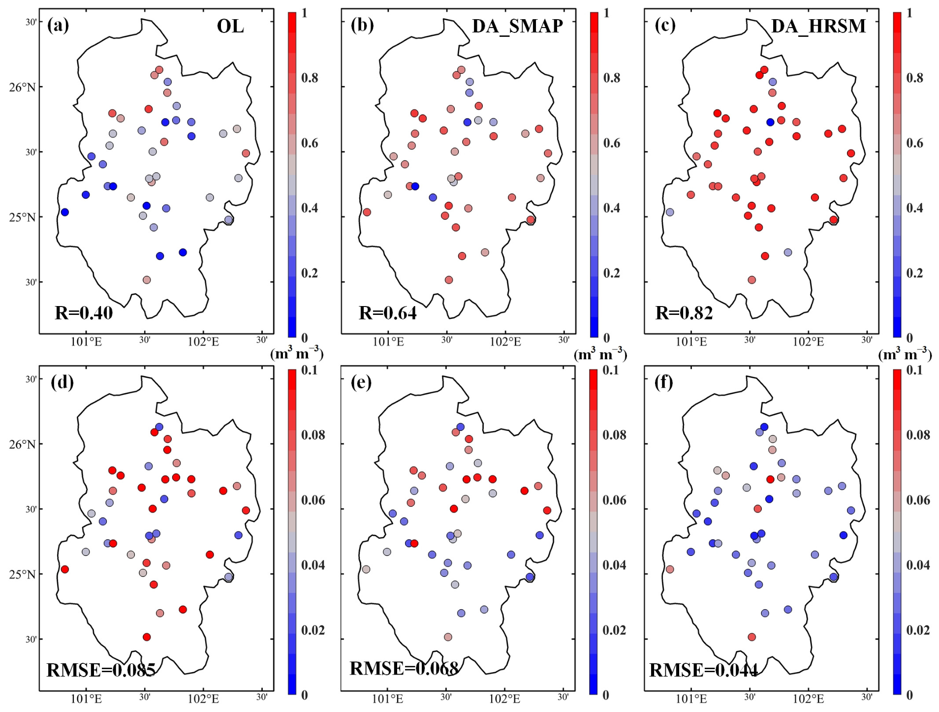
Given the high spatial resolution of the remote sensing data and DA-based SM simulations, the station observations were considered representative of conditions at the pixel scale. This study independently validated the DA results using 40 SM observation stations in Chuxiong City. Figure 4 illustrates the RMSE and R patterns for the OL, DA_SMAP, and DA_HRSM methods compared with in situ measurements in Chuxiong City. This study focuses on the differences in SSM (10 cm) simulations among the OL, DA_SMAP, and DA_HRSM methods. The average R and RMSE values for the OL method are 0.44 and 0.075 m³ m⁻³. These discrepancies are primarily attributed to the default soil hydraulic properties (e.g., sand, clay, silt content, bulk density, and saturated hydraulic conductivity) used in the Noah-MP model, which introduce biases in SSM simulation. Additionally, differences in representativeness between the in situ observations and the model grids add uncertainty to the validation process. The estimation of DA_SMAP is better than that of OL (ΔR ~ 0.19). The results indicate that SMAP retrievals provide additional information for SM estimates through the DA method. Compared to DA_SMAP, the assimilation of HRSM further enhances the performance of the Noah-MP model, with average R and RMSE values reaching 0.81 and 0.037 m³ m⁻³, respectively. Figure 5 further evaluates the simulation accuracy of RZSM (40 cm). The results show that assimilating SSM data has an indirect positive impact on RZSM. The mean RMSE of RZSM retrievals from DA_HRSM is 0.044 m³ m⁻³, which is 35.29% lower than the RMSE of 0.068 m³ m⁻³ from DA_SMAP. Overall, the assimilation of HRSM significantly improves both the simulation capability and the validation accuracy of the Noah-MP model for SSM and RZSM.

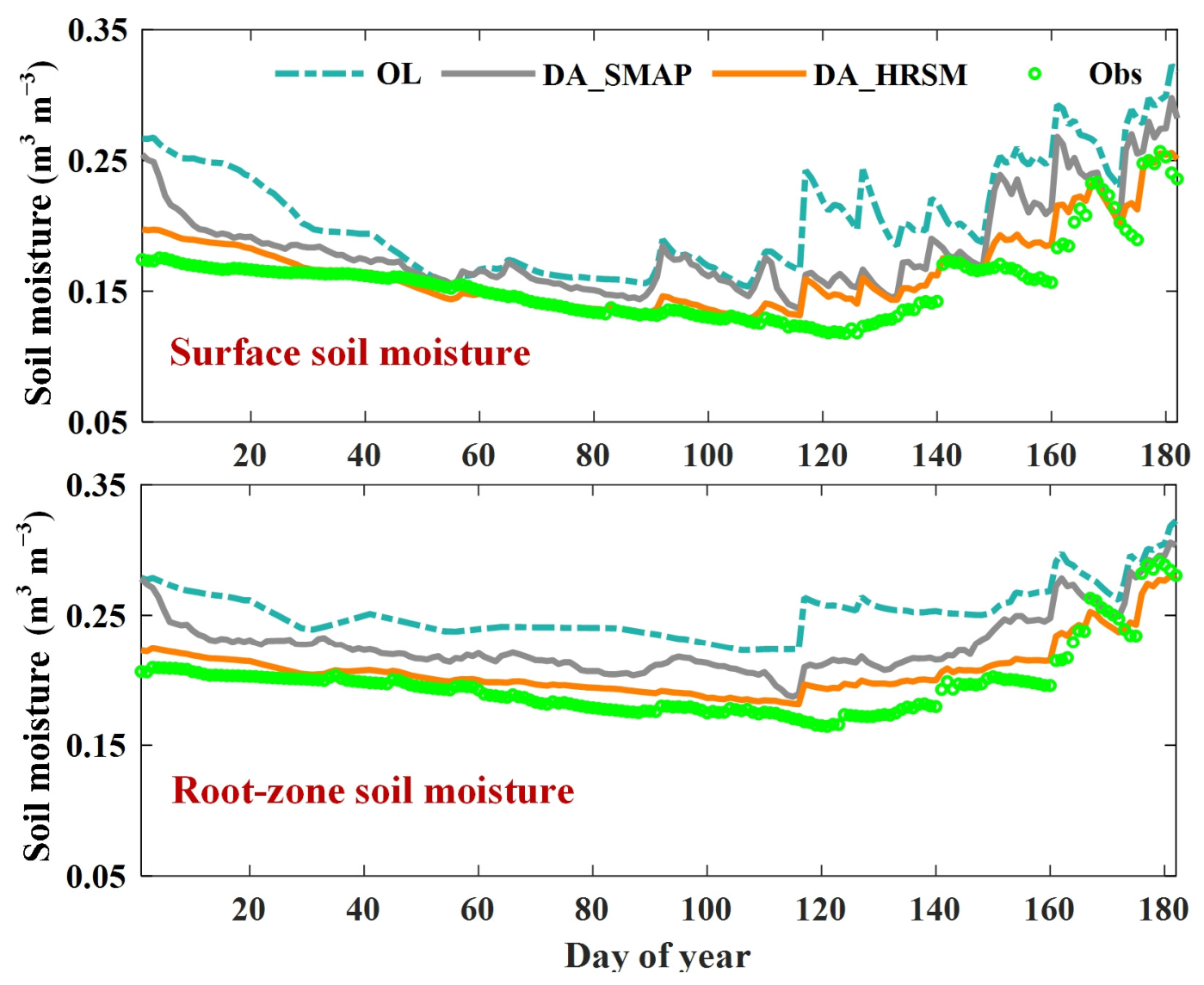
Figure 6 presents the time series of SSM and RZSM generated by the OL, DA_SMAP, and DA_HRSM methods in Chuxiong City. The results indicate that the Noah-MP model tends to overestimate both SSM and RZSM compared to observations, suggesting that the model struggles to capture the dynamic characteristics of SM during dry years. From January to April, SM gradually decreases due to limited precipitation. Although the Noah-MP model captures this temporal trend, the simulated values remain consistently overestimated. Compared to the OL method, assimilating SMAP SM improves the simulation accuracy. However, due to the coarse spatial resolution of SMAP, it fails to capture the fine-scale spatial variability of soil characteristics. As a result, the DA_SMAP method still slightly overestimates RZSM. In contrast, assimilating HRSM data further improves the simulation accuracy of both SSM and RZSM, yielding results more consistent with observations. The DA_HRSM simulations capture a gradual decline in SM from January to April due to drought conditions, followed by an increase beginning in May as precipitation becomes more abundant.

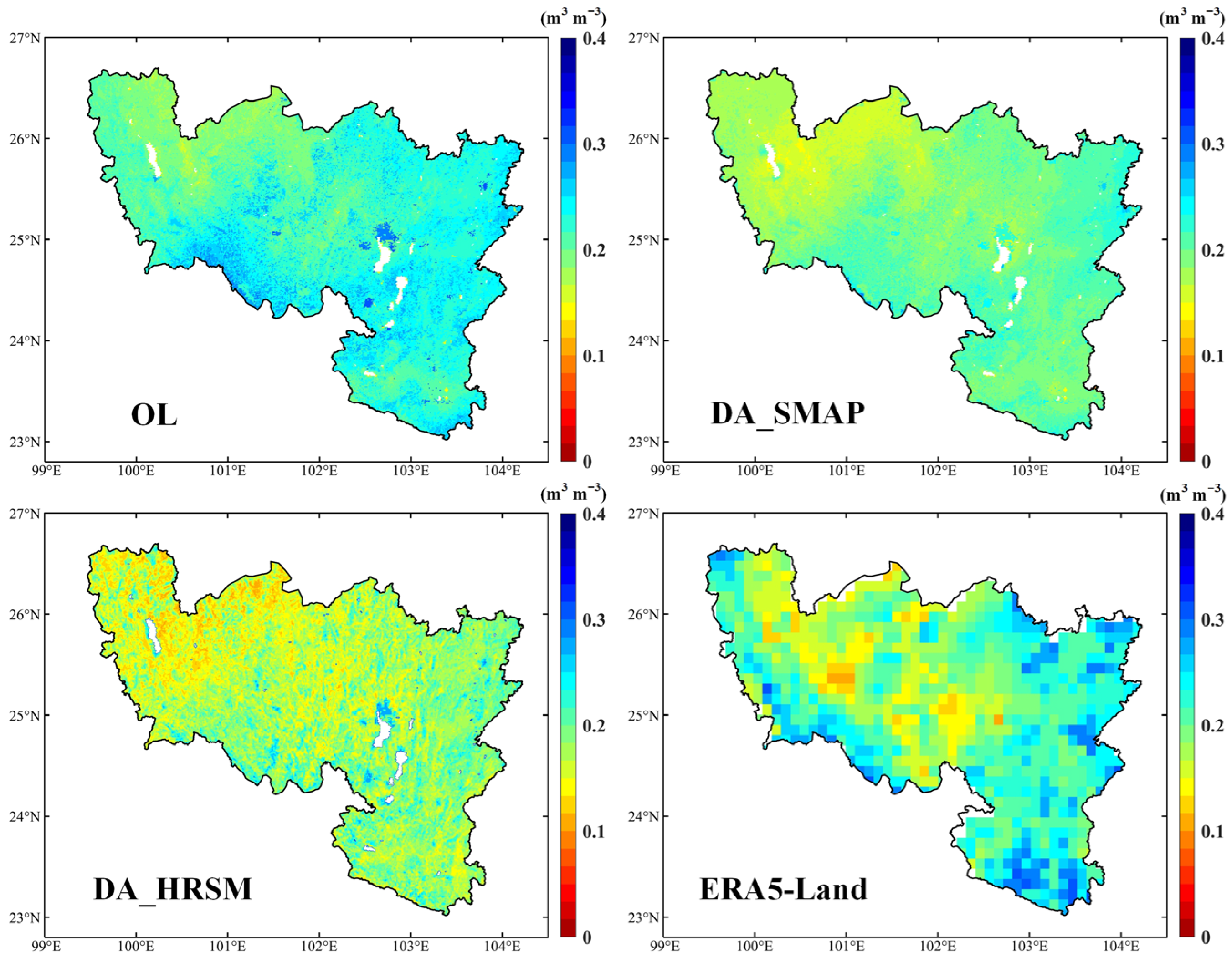
Figure 7 shows the SSM estimated by the OL, DA_SMAP, and DA_HRSM methods, along with ERA5-Land data. Analysis shows that DA_SMAP alters the spatial distribution pattern of SSM. Although DA_SMAP improves SM estimation compared to the OL method, it weakens the spatial detail of the distribution. In contrast, DA_HRSM better preserves the continuity of SM spatial patterns. Its ability to capture high-resolution details in simulated SM outperforms that of the OL, DA_SMAP, and ERA5-Land methods. The spatial distribution of SM simulated by DA_HRSM shows higher consistency with high-resolution driving factors such as precipitation, elevation, land cover type, and LAI, indicating that the results more accurately capture the fine-scale spatial variability of SM.

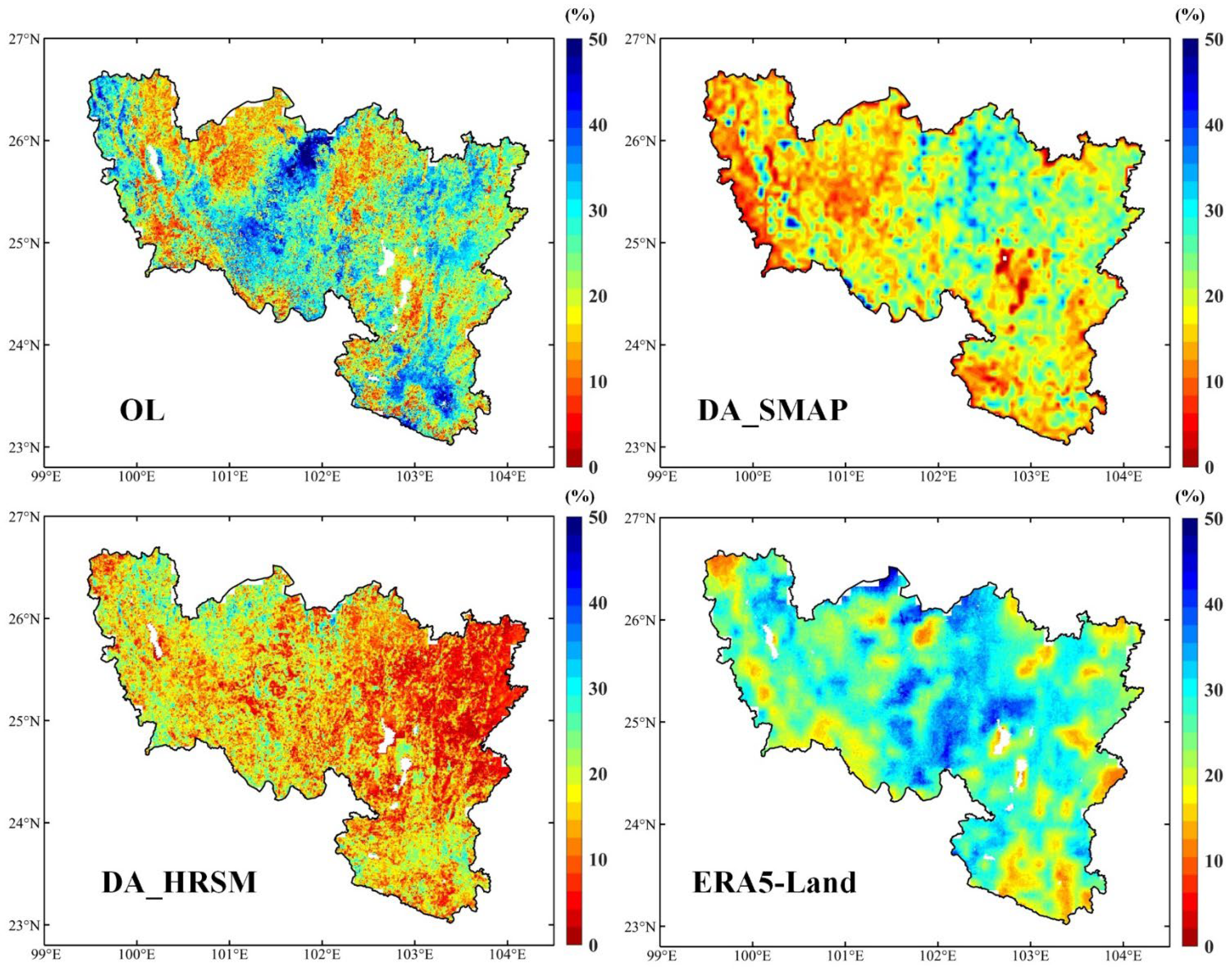
The TCH method was used to evaluate the relative uncertainty of the four datasets. Figure 8 illustrates the spatial distribution of relative uncertainty in SM simulations from the OL, DA_SMAP, and DA_HRSM methods, as well as from ERA5-Land data. Overall, the DA_HRSM method exhibited the lowest relative uncertainty across most areas of central Yunnan, while the ERA5-Land product showed the highest. The high relative uncertainty of the ERA5-Land data is attributed to its coarse spatial resolution (9 km). Additionally, compared to DA_HRSM, ERA5-Land SM tends to be overestimated in the southeastern part of central Yunnan and underestimated in Chuxiong City. In contrast to both OL and DA_SMAP, DA_HRSM significantly reduces the uncertainty in SM estimation, particularly in central Yunnan Province.

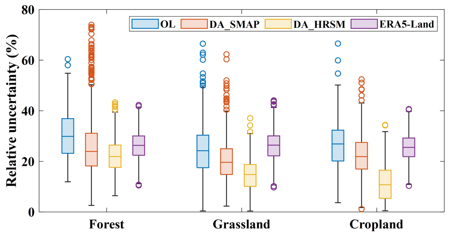
Figure 9 shows box plots of the relative uncertainty in SM simulations for forest, grassland, and cropland. The relative uncertainties of SM estimates from the OL, DA_SMAP, DA_HRSM, and ERA5-Land methods are 25.51%, 20.87%, 16.22%, and 25.86%, respectively. Most of the uncertainties in the OL method range from approximately 8.05% to 38.91%, while those in the DA_SMAP method fall between approximately 10.32% and 32.52%. In addition, the uncertainties in the DA_HRSM and ERA5-Land products mostly range from approximately 7.62% to 25.64% and 16.25% to 35.71%, respectively. Compared to the OL and DA_SMAP methods, the relative uncertainty in SM simulations using the DA_HRSM method is reduced by approximately 7.29% and 4.65%, respectively. The results also indicate that the relative uncertainty in SM simulated by the DA_HRSM method is higher in forest than in grassland and cropland. This is because forests typically have deep and dense canopies, making it difficult for microwave or optical signals to penetrate the thick vegetation layer and reach the soil surface, thereby increasing the uncertainty of SM estimation in the SWI calculation.

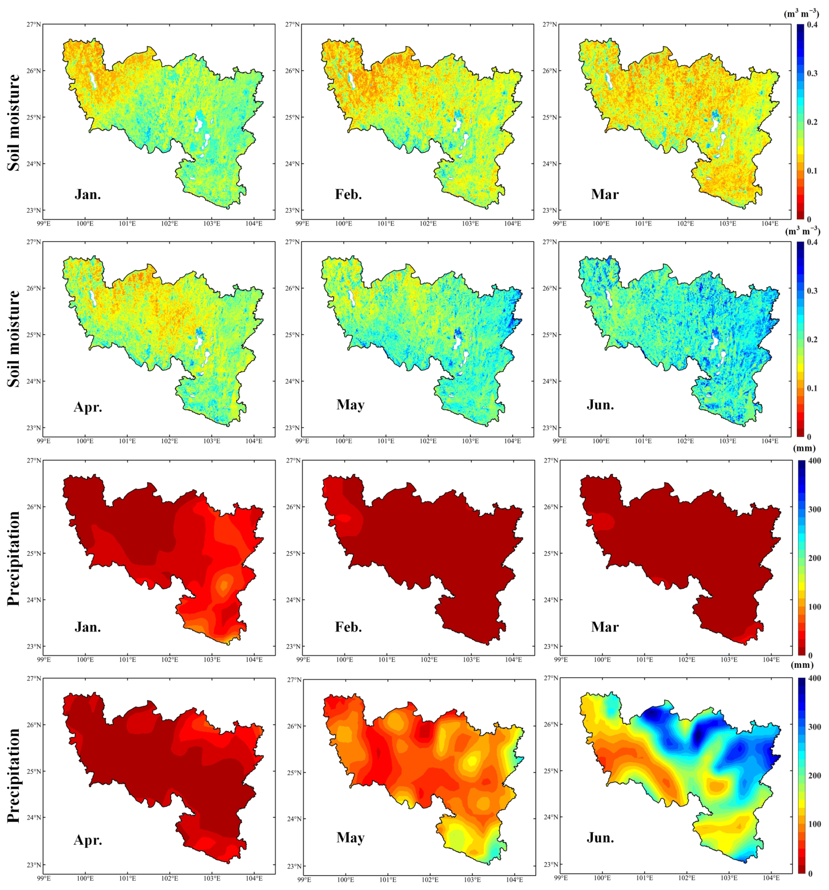
The spatial distribution of SM simulated by the DA_HRSM method and the corresponding precipitation from January to June are shown in Figure 10. The results indicate that simulated SM in central Yunnan gradually decreased from January to March, reaching its lowest level in March due to the lack of precipitation. A gradual increase in SM was observed from April to June, driven by rising precipitation. The spatial distribution of SM closely corresponds to that of precipitation. In the southeastern part of central Yunnan, high SM values align with increased precipitation. Additionally, during March and April, the persistent drought conditions in Chuxiong City (reflected by low SM values) are associated with minimal precipitation. This suggests that assimilating HRSM enables better capture of the spatiotemporal characteristics of SM during drought periods and is consistent with precipitation patterns.

4.2. Agricultural and Drought Monitoring Applications

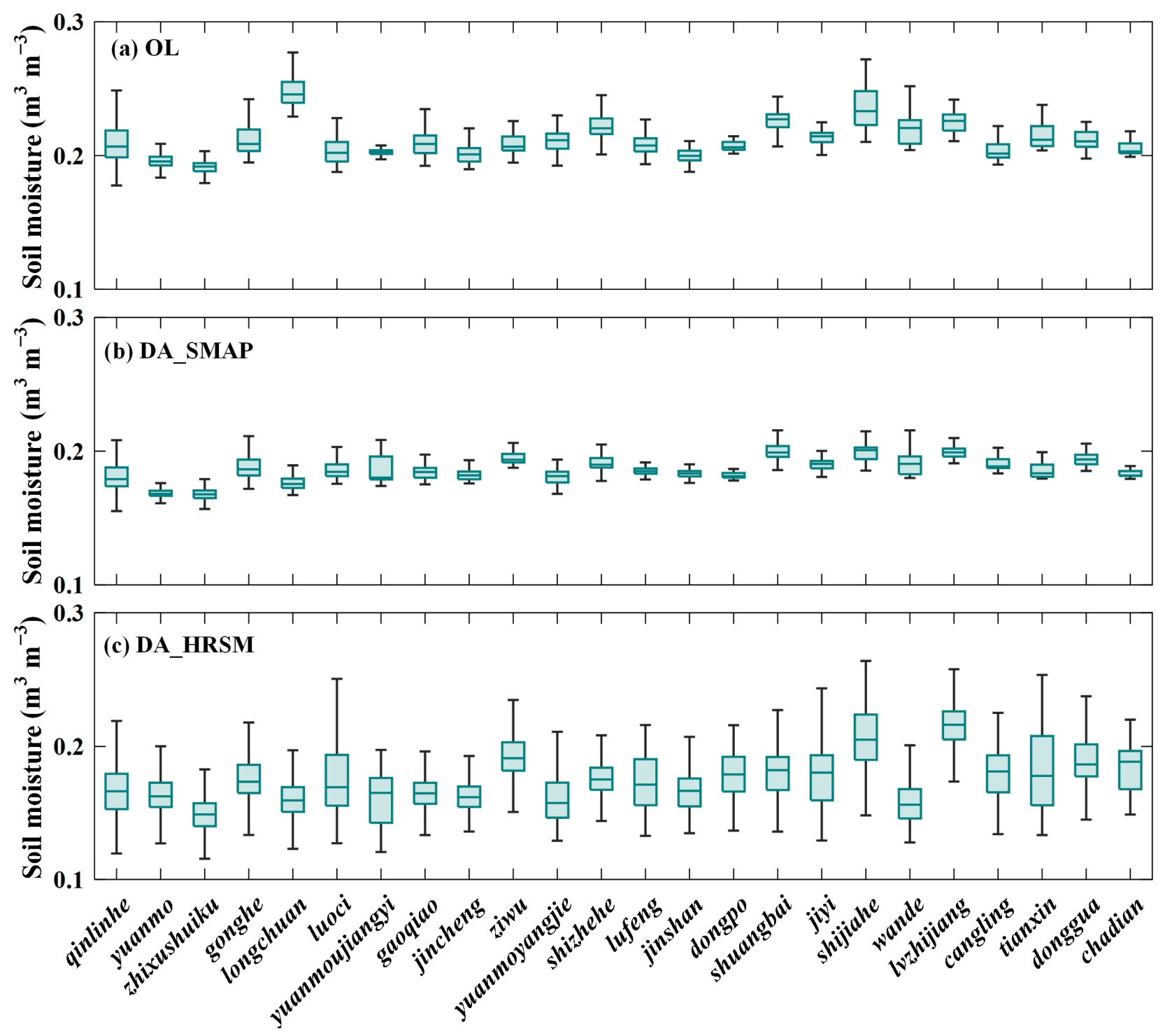
In agricultural applications, SM not only needs high spatial resolution and spatiotemporal continuity but also the ability to capture changes driven by climate variability and human activities, such as irrigation. The SMAP SM products have been demonstrated to capture large-scale irrigation signals in arid and semi-arid regions [47]. However, due to its relatively coarse observational footprint, SMAP still cannot distinguish the SM distribution at the field scale. To further assess the robustness of the DA methods, SM simulations from the OL, DA_SMAP, and DA_HRSM methods across different irrigation districts in Chuxiong City are summarized in Figure 11. Box plots were used to show the mean SM values and their distribution ranges. The largest irrigation district is Qinlinhe, with an area of 941.97 km², while the smallest is Chadian, with an area of 8.13 km². The districts are arranged in descending order by area.

Overall, the OL method exhibits higher SM values in different irrigation districts, especially in the Longchun and Shijiahe irrigation districts. Most of the SM values from the OL method range from approximately 0.18 m³ m⁻³ to 0.26 m³ m⁻³. Assimilating SMAP and HRSM data generally reduces the simulated SM values. Most of the SM values from the DA_SMAP and DA_HRSM methods range from approximately 0.18 m³ m⁻³ to 0.22 m³ m⁻³ and approximately 0.13 m³ m⁻³ to 0.24 m³ m⁻³, respectively. Compared to DA_SMAP, the DA_HRSM method simulates a broader range of SM distributions. This suggests that compared to assimilating SMAP data, the DA_HRSM method provides SM estimates with finer spatial detail at the irrigation district scale. This offers a promising approach for high-resolution agricultural water monitoring.

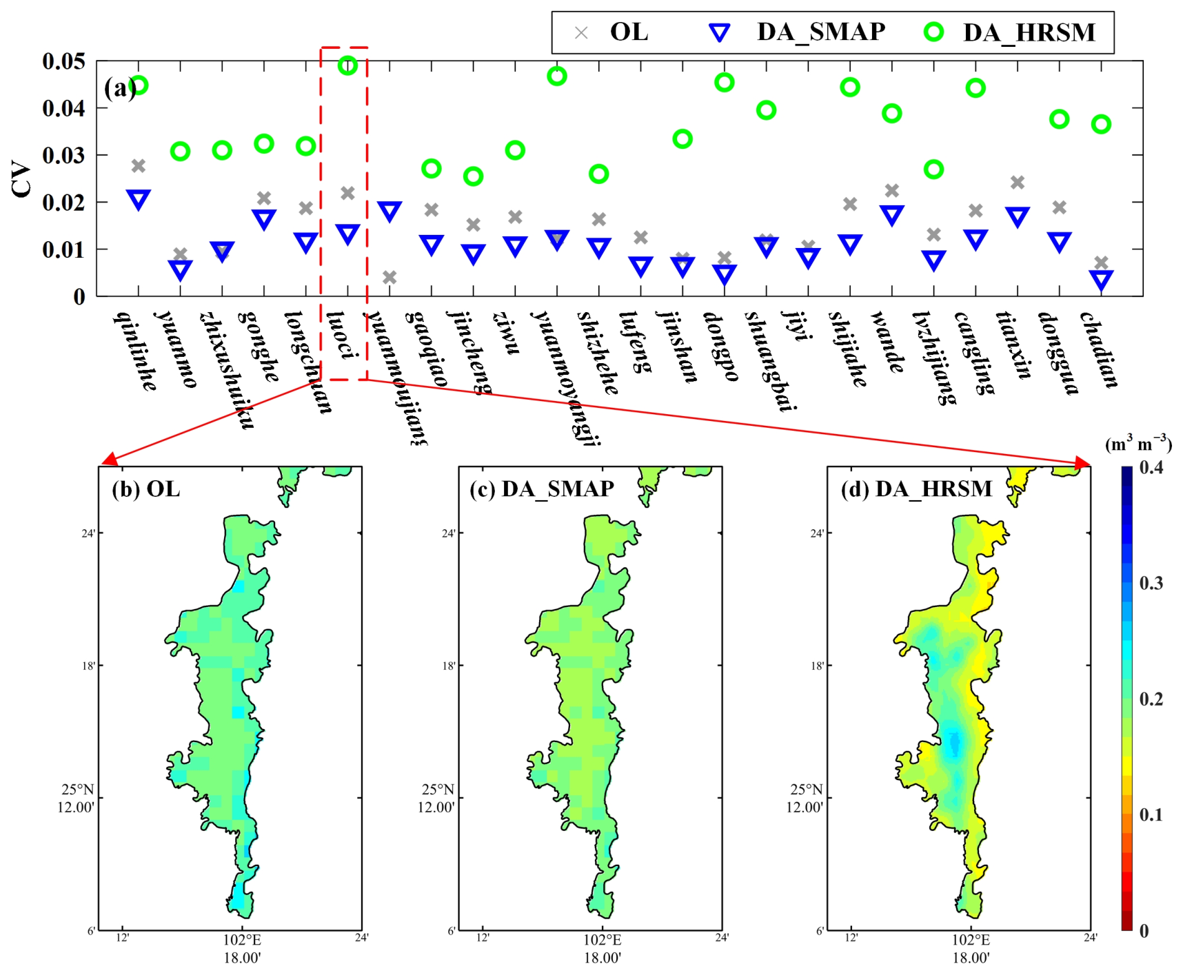
To further assess the spatial heterogeneity of estimated SM, the CV was used to evaluate SM variability across different irrigation districts (Figure 12). The results show that the OL method simulates lower spatial heterogeneity of SM, indicating that the 1 km SM simulation by the Noah-MP model struggles to capture the spatial distribution characteristics of SM at the irrigation district scale. By assimilating SMAP SM, the DA_SMAP method reduces the spatial heterogeneity of simulated SM. This suggests that while the assimilation of 9 km SM improves SSM simulation accuracy, it reduces the ability to capture SM distribution at the irrigation district scale. In contrast, the assimilation of HRSM data increases spatial heterogeneity. The CV values for DA_HRSM in the 20 irrigation districts are nearly twice those of DA_SMAP. Figure 12 further illustrates the distribution characteristics of SM in the Luoci irrigation district. The results show that DA_HRSM better captures the high-resolution distribution of SM, with higher values observed in the central part of the irrigation district. High-resolution SSM simulations through DA methods can effectively support irrigation system development, optimized water resource allocation, and sustainable water use. The results also indicate that the fine-scale spatial characteristics of DA_HRSM estimates are weakened, leading to smoother SM simulations in irrigated areas. This is because during the calculation of the Kalman gain, the model states at a 1 km resolution reduce the representation of fine-scale spatial variability in SM (Figure 3).

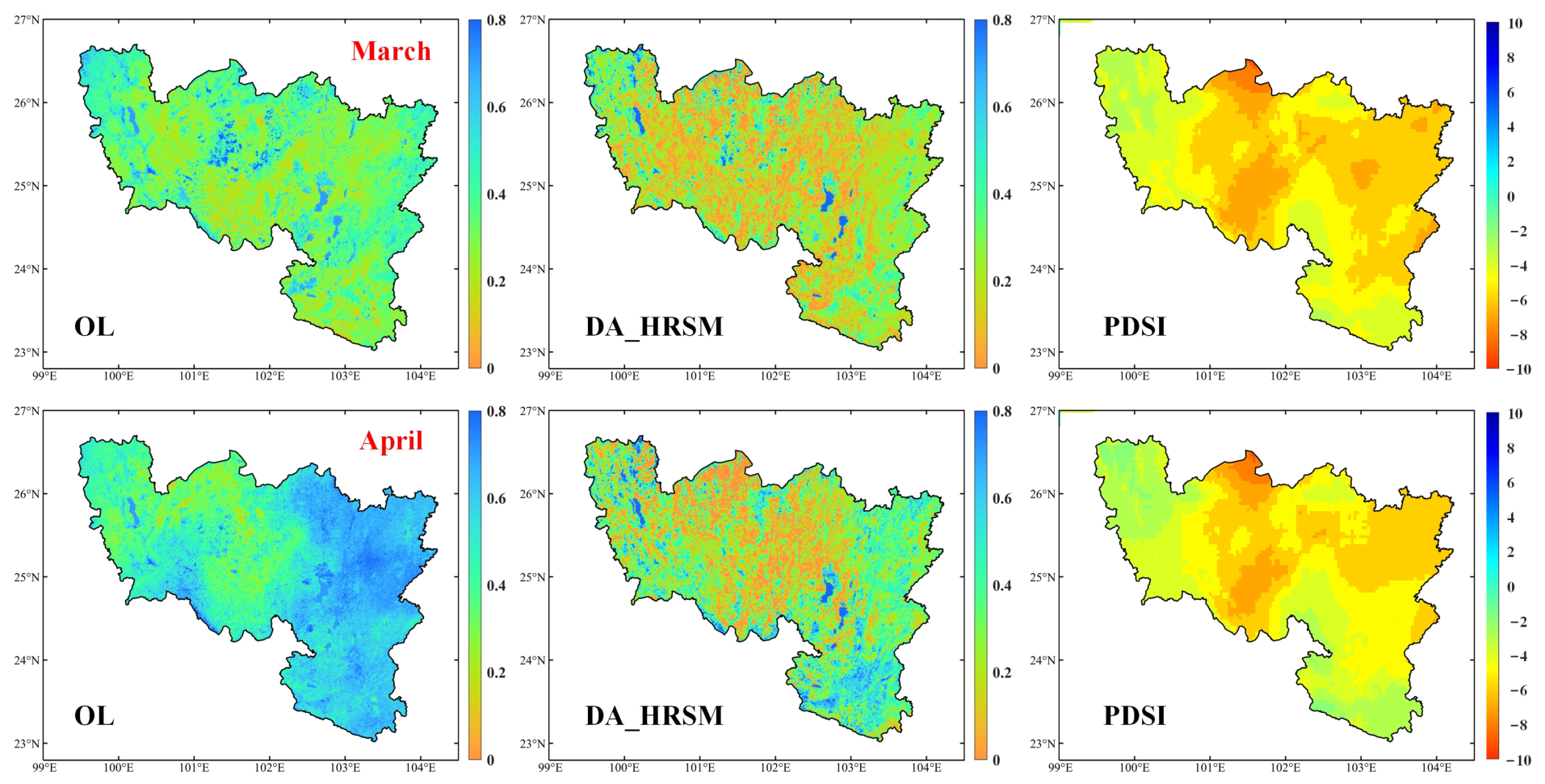
This study further evaluates the impact of HRSM assimilation on extreme climate and hydrological events. The SM simulated by the OL and DA_HRSM methods will be used to calculate the SMCI drought index. Figure 13 shows the spatial patterns of the SMCI index, derived from SSM estimates based on the OL and DA_HRSM methods. A comparison with OL simulations reveals that the DA_HRSM method provides a better representation of drought distribution in central Yunnan, particularly during March 2024. The corresponding spatial distribution of PDSI is also shown in Figure 13. Analysis shows that most areas in central Yunnan experienced moderate drought conditions (PDSI < −2), whereas Chuxiong City and its eastern regions suffered from extreme drought (PDSI < −4). The spatial pattern of drought identified by the DA_HRSM method aligns well with that of the PDSI. The extent of extreme drought in April decreased compared to March, which is consistent with the DA_HRSM simulation results. Overall, the assimilation of HRSM provides more detailed spatial SM information and accurately captures the extreme drought conditions in central Yunnan during the spring of 2024.

5. Discussions

5.1. Uncertainty of the HRSM

In the estimation of HRSM, to ensure spatial consistency, all input datasets were progressively resampled to a target spatial resolution (e.g., 1 km or 16 m). It should be noted that resampling does not generate new spatial information from coarse-resolution products but is used to facilitate multi-source data integration. Coarse-resolution data provide regional-scale SM constraints, whereas high-resolution data capture local spatial heterogeneity. Although the resampling process inevitably introduces uncertainty due to unresolved sub-grid variability, this uncertainty is particularly pronounced over heterogeneous land surfaces, where strong spatial variability cannot be fully represented by coarse-resolution observations. Nevertheless, this approach enables effective reconstruction of fine-scale spatial patterns while maintaining large-scale consistency. ESTARFM was designed for the fusion of optical reflectance data based on assumptions of temporal continuity and spatial homogeneity within land cover types. In this study, we extend its application to SM data fusion, where similar spatiotemporal consistency assumptions are approximately valid at short temporal scales, although additional uncertainties may be introduced due to the nonlinear dynamics of SM.

In the HRSM data, the optical and NIR remote sensing bands used to capture high-resolution features are generally more sensitive to surface soil and vegetation states, while their direct response to SM content is relatively limited. Consequently, the HRSM estimates are derived by fitting a linear regression model to in situ SM observations, which introduces uncertainties in regions where ground-based SM measurements are unavailable. To further evaluate the spatial transferability of the HRSM regression model, a five-fold cross-validation was conducted. The observation sites were randomly partitioned into five subsets. In each iteration, four subsets were used to develop the regression model, while the remaining subset was used for independent validation. This procedure was repeated until each subset had been used once for validation. The resulting R and RMSE values from the five validation folds are presented in

Table 2. Performance of SM simulation based on five-fold cross-validation.

Metrics	Fold 1	Fold 2	Fold 3	Fold 4	Fold 5
RMSE	0.037	0.032	0.042	0.035	0.034
R	0.79	0.83	0.74	0.79	0.81

. The model achieved mean R and RMSE values of 0.79 and 0.036 m³ m⁻³, respectively. Notably, Fold 3 exhibited a relatively lower R and higher RMSE compared to the other folds. Overall, the regression model demonstrates consistent performance across different subsets of SM observations, indicating stable spatial transferability. In future work, machine learning approaches could be employed to train and generalize SM estimates from station observations, thereby potentially reducing uncertainties in SM products.

5.2. Uncertainty of the DA_HRSM Method

Although assimilating HRSM data provides fine-scale SM characteristics, the DA framework proposed in this study still exhibits uncertainties. Firstly, the uncertainties in Noah-MP model simulations mainly stem from the forcing data, model parameters, and model structure. In this study, meteorological variables from the CMFD product were used as high-resolution forcing inputs for the Noah-MP simulations. However, uncertainties in precipitation, particularly over complex mountainous terrain, may introduce biases in SM simulations [48]. In addition, structural and parameter uncertainties inherent in the Noah-MP model may further contribute to simulation errors. The Noah-MP model uses fixed input parameters for vegetation and soil types to simulate vegetation dynamics and SM and does not capture the spatiotemporal variability of vegetation phenology and soil properties in complex mountain terrain. Therefore, the uncertainties in simulating hydrological processes with the Noah-MP model in complex mountainous regions need to be further evaluated.

Secondly, HRSM data and the TCH method were used to estimate observation errors within the DA framework and update the Kalman gain. This approach provided refined spatial features and error information for SM within the DA framework. However, to ensure the computational efficiency of the Noah-MP model, the DA method was conducted at a spatial resolution of 1 km. During this process, the fine-scale spatial characteristics of HRSM were weakened, resulting in smoother SM simulations in irrigated areas and introducing uncertainty into the SM estimates (Figure 12). Although the TCH method assumes that the errors of the input datasets are mutually uncorrelated, HRSM partially inherits information from SMAP, which may introduce correlation and thereby affect the estimation of relative uncertainty. At present, this method is applied only to SM DA. Future work should further evaluate its applicability to additional assimilated variables, such as LAI and land surface temperature, in order to improve its scalability and general applicability. In addition, we will extend the DA_HRSM framework to multi-year simulations and evaluate its performance under both wet and dry conditions to further assess its robustness and generalizability.

Overall, the DA_HRSM framework delivers highly accurate, spatiotemporally continuous multi-layer SM data. This capability is vital for agricultural applications and drought monitoring. In the future, DA methods will be applied across diverse hydroclimatic conditions, including both drought and wet periods, and will focus on coupling with crop models and their applications in yield estimation, drought forecasting, and other related areas.

6. Conclusions

In this study, a daily 16 m SM dataset was developed using multi-source remote sensing data (e.g., SMAP, HJ-2, Sentinel-2, and Gaofen-6) and the ESTARFM. Thereafter, a high-resolution DA system is generated, based on the Noah-MP model, the EnKF framework, and the TCH method. In this system, the relative uncertainties of HRSM derived from the TCH method were used to compute the observation error and Kalman gain in the EnKF method, which subsequently updated SSM and RZSM estimates at a 16 m resolution. The developed DA_HRSM framework was tested during the spring drought period in central Yunnan Province, China.

The results indicate that the assimilation of remotely sensed LAI and HRSM into the Noah-MP model improves SSM and RZSM estimates. The SM estimates from the DA_HRSM method agree well with in situ observations in Chuxiong City. The RMSE of SSM retrievals from DA_HRSM is 0.037 m³ m⁻³, which is a 50.67% reduction of the RMSE of 0.075 m³ m⁻³ from the OL method. The DA_HRSM system improves the SM estimates compared to the OL and DA_SMAP methods and effectively captures fine-scale spatial characteristics of SM. The relative uncertainties of SM retrievals from the DA_HRSM method are also compared with those from the OL, DA_SMAP, and ERA5-Land products. The smallest uncertainties are obtained from DA_HRSM in most areas of central Yunnan, followed by DA_SMAP, OL, and ERA5-Land products.

The estimated HRSM was further analyzed in different irrigation districts of Chuxiong City. The results show that the assimilation of SMAP SM reduces the ability to capture the spatial distribution of SM at the irrigation district scale. Compared to the OL and DA_SMAP methods, the assimilation of HRSM shows higher heterogeneity and better captures the soil characteristics of agricultural fields. Finally, assimilating HRSM data significantly improved the capability to monitor drought conditions and was consistent with PDSI. The assimilation of HRSM more accurately matched the extreme drought conditions during the spring drought in central Yunnan in 2024.

References

1. Abowarda, A.S.; Bai, L.; Zhang, C.; Long, D.; Li, X.; Huang, Q.; Sun, Z. Generating surface soil moisture at 30 m spatial resolution using both data fusion and machine learning toward better water resources management at the field scale. Remote Sens. Environ. 2021, 255, 112301. [Google Scholar] [CrossRef]
2. Zeri, M.; Williams, K.; Cunha, A.P.M.A.; Cunha-Zeri, G.; Vianna, M.S.; Blyth, E.M.; Marthews, T.R.; Hayman, G.D.; Costa, J.M.; Marengo, J.A.; et al. Importance of including soil moisture in drought monitoring over the Brazilian semiarid region: An evaluation using the JULES model, in situ observations, and remote sensing. Clim. Atmos. Sci. 2022, 5, 7. [Google Scholar]
3. Babaeian, E.; Paheding, S.; Siddique, N.; Devabhaktuni, V.K.; Tuller, M. Estimation of root zone soil moisture from ground and remotely sensed soil information with multisensor data fusion and automated machine learning. Remote Sens. Environ. 2021, 260, 112434. [Google Scholar] [CrossRef]
4. Dirmeyer, P.A.; Halder, S. Sensitivity of numerical weather forecasts to initial soil moisture variations in CFSv2. Weather Forecast. 2016, 31, 1973–1983. [Google Scholar] [CrossRef]
5. Kannenberg, S.A.; Anderegg, W.R.L.; Barnes, M.L.; Dannenberg, M.P.; Knapp, A.K. Dominant role of soil moisture in mediating carbon and water fluxes in dryland ecosystems. Nat. Geosci. 2024, 17, 38–43. [Google Scholar] [CrossRef]
6. Li, Q.; Shi, G.; Shangguan, W.; Nourani, V.; Li, J.; Li, L.; Huang, F.; Zhang, Y.; Wang, C.; Wang, D.; et al. A 1 km daily soil moisture dataset over China using in situ measurement and machine learning. Earth Syst. Sci. Data 2022, 14, 5267–5286. [Google Scholar] [CrossRef]
7. Li, S.; Han, Y.; Li, C.; Wang, J. A novel framework for multi-layer soil moisture estimation with high spatio-temporal resolution based on data fusion and automated machine learning. Agric. Water Manag. 2024, 306, 109173. [Google Scholar]
8. Wagner, W.; Hahn, S.; Kidd, R.; Melzer, T.; Bartalis, Z.; Hasenauer, S.; Figa-Saldaña, J.; de Rosnay, P.; Jann, A.; Schneider, S.; et al. The ASCAT soil moisture product: A review of its specifications, validation results, and emerging applications. Meteorol. Z. 2013, 22, 5–33. [Google Scholar] [CrossRef]
9. Kerr, Y.H.; Waldteufel, P.; Richaume, P.; Wigneron, J.P.; Ferrazzoli, P.; Mahmoodi, A.; Al Bitar, A.; Cabot, F.; Gruhier, C.; Juglea, S.E.; et al. The SMOS soil moisture retrieval algorithm. IEEE Trans. Geosci. Remote Sens. 2012, 50, 1384–1403. [Google Scholar] [CrossRef]
10. Njoku, E.G.; Jackson, T.J.; Lakshmi, V.; Chan, T.K.; Nghiem, S.V. Soil moisture retrieval from AMSR-E. IEEE Trans. Geosci. Remote Sens. 2003, 41, 215–229. [Google Scholar] [CrossRef]
11. Seo, E.; Lee, M.I.; Reichle, R.H. Assimilation of SMAP and ASCAT soil moisture retrievals into the JULES land surface model using the Local Ensemble Transform Kalman Filter. Remote Sens. Environ. 2021, 253, 112222. [Google Scholar] [CrossRef]
12. Zhu, Y.; Guo, F.; Yang, W.; Zhang, Z.; Li, Z.; Wu, Z.; Zhang, X. An algorithm for downscaling SMAP soil moisture to 3 km using CYGNSS observations. IEEE Trans. Geosci. Remote Sens. 2025, 63, 4406210. [Google Scholar] [CrossRef]
13. Lei, F.; Senyurek, V.; Kurum, M.; Gurbuz, A.C.; Boyd, D.; Moorhead, R.; Crow, W.T.; Eroglu, O. Quasi-global machine learning-based soil moisture estimates at high spatio-temporal scales using CYGNSS and SMAP observations. Remote Sens. Environ. 2022, 276, 113041. [Google Scholar]
14. Yan, Q.; Chen, Y.; Pan, Y.; Jin, S.; Huang, W. A modified hierarchical vision transformer for soil moisture retrieval from CYGNSS data. Water Resour. Res. 2026, 62, e2024WR039476. [Google Scholar]
15. Pan, X.; Chen, D.; Pan, B.; Huang, X.; Yang, K.; Piao, S.; Zhou, T.; Dai, Y.; Chen, F.; Li, X. Evolution and prospects of Earth system models: Challenges and opportunities. Earth Sci. Rev. 2025, 260, 104986. [Google Scholar]
16. Zeng, Q.; Zhang, M.; Dai, Y.; Zeng, X. Research on Earth system models and numerical simulations. J. Meteorol. Res. 2025, 39, 467–484. [Google Scholar] [CrossRef]
17. Arsenault, K.R.; Nearing, G.S.; Wang, S.; Yatheendradas, S.; Peters-Lidard, C.D. Parameter sensitivity of the Noah-MP land surface model with dynamic vegetation. J. Hydrometeorol. 2018, 19, 815–830. [Google Scholar] [CrossRef]
18. Zheng, H.; Yang, Z.L.; Lin, P.R.; Wei, J.F.; Wu, W.Y.; Li, L.C.; Zhao, L.; Wang, S. On the sensitivity of the precipitation partitioning into evapotranspiration and runoff in land surface parameterizations. Water Resour. Res. 2019, 55, 95–111. [Google Scholar] [CrossRef]
19. Zhang, Z.; Barlage, M.; Chen, F.; Li, Y.; Helgason, W.; Xu, X.; Liu, X.; Li, Z. Joint modeling of crop and irrigation in the central United States using the Noah-MP land surface model. J. Adv. Model. Earth Syst. 2020, 12, e2020MS002159. [Google Scholar]
20. Xia, Y.; Hao, Z.; Shi, C.; Li, Y.; Meng, J.; Xu, T.; Wu, X.; Zhang, B. Regional and global land data assimilation systems: Innovations, challenges, and prospects. J. Meteorol. Res. 2019, 33, 159–189. [Google Scholar] [CrossRef]
21. Li, X.; Liu, F.; Ma, C.; Hou, J.; Zheng, D.; Ma, H.; Bai, Y.; Han, X.; Vereecken, H.; Yang, K.; et al. Land data assimilation: Harmonizing theory and data in land surface process studies. Rev. Geophys. 2024, 62, e2022RG000801. [Google Scholar] [CrossRef]
22. Kumar, S.V.; Mocko, D.M.; Wang, S.; Peters-Lidard, C.D.; Borak, J. Assimilation of remotely sensed leaf area index into the Noah-MP land surface model: Impacts on water and carbon fluxes and states over the continental United States. J. Hydrometeorol. 2019, 20, 1359–1377. [Google Scholar] [CrossRef]
23. Nie, W.; Zaitchik, B.F.; Rodell, M.; Kumar, S.V.; Arsenault, K.R.; Li, B.; Getirana, A. Assimilating GRACE into a land surface model in the presence of an irrigation-induced groundwater trend. Water Resour. Res. 2019, 55, 11274–11294. [Google Scholar]
24. Zhao, L.; Yang, Z.L.; Hoar, T.J. Global soil moisture estimation by assimilating AMSR-E brightness temperatures in a coupled CLM4–RTM–DART system. J. Hydrometeorol. 2016, 17, 2431–2454. [Google Scholar]
25. Ahmad, J.A.; Forman, B.A.; Kumar, S.V. Soil moisture estimation in South Asia via assimilation of SMAP retrievals. Hydrol. Earth Syst. Sci. 2022, 26, 2221–2243. [Google Scholar] [CrossRef]
26. He, X.; Liu, S.; Xu, T.; Yu, K.; Gentine, P.; Zhang, Z.; Xu, Z.; Jiao, D.; Wu, D. Improving predictions of evapotranspiration by integrating multi-source observations and land surface model. Agric. Water Manag. 2022, 272, 107827. [Google Scholar] [CrossRef]
27. He, X.; Liu, S.; Bateni, S.M.; Xu, T.; Jun, C.; Kim, D.; Li, X.; Song, L.; Zhao, L.; Xu, Z.; et al. Innovative approach for estimating evapotranspiration and gross primary productivity by integrating land data assimilation, machine learning, and multi-source observations. Agric. For. Meteorol. 2024, 355, 110136. [Google Scholar] [CrossRef]
28. Lan, T.; Yan, X. Analysis of drought characteristics and causes in Yunnan Province in the last 60 years (1961–2020). J. Hydrometeorol. 2024, 25, 177–190. [Google Scholar] [CrossRef]
29. Zhao, J.; Xu, T.; Xiao, J.; Liu, S.; Mao, K.; Song, L.; Yao, Y.; He, X.; Feng, H. Responses of water use efficiency to drought in Southwest China. Remote Sens. 2020, 12, 199. [Google Scholar] [CrossRef]
30. He, J.; Yang, K.; Tang, W.; Lu, H.; Qin, J.; Chen, Y.Y.; Li, X. The first high-resolution meteorological forcing dataset for land process studies over China. Sci. Data 2020, 7, 25. [Google Scholar] [CrossRef] [PubMed]
31. Das, N.N.; Entekhabi, D.; Dunbar, R.S.; Chaubell, M.J.; Colliander, A.; Yueh, S.; Jagdhuber, T.; Chen, F.; Crow, W.; O’Neill, P.E.; et al. The SMAP and Copernicus Sentinel 1A/B microwave active-passive high resolution surface soil moisture product. Remote Sens. Environ. 2019, 233, 111380. [Google Scholar]
32. Li, Z.; He, W.; Cheng, M.; Hu, J.; Yang, G.; Zhang, H. SinoLC-1: The first 1 m resolution national-scale land-cover map of China created with a deep learning framework and open-access data. Earth Syst. Sci. Data 2023, 15, 4749–4780. [Google Scholar] [CrossRef]
33. Niu, G.-Y.; Yang, Z.-L.; Mitchell, K.E.; Chen, F.; Ek, M.B.; Barlage, M.; Kumar, A.; Manning, K.; Niyogi, D.; Rosero, E.; et al. The community Noah land surface model with multiparameterization options (Noah-MP): 1. Model description and evaluation with local-scale measurements. J. Geophys. Res. Atmos. 2011, 116, D12109. [Google Scholar]
34. Liu, X.; Chen, F.; Barlage, M.; Zhou, G.; Niyogi, D. Noah-MP-Crop: Introducing dynamic crop growth in the Noah-MP land surface model. J. Geophys. Res. Atmos. 2016, 121, 13953–13972. [Google Scholar]
35. He, C.; Valayamkunnath, P.; Barlage, M.; Chen, F.; Gochis, D.; Cabell, R.; Schneider, T.; Rasmussen, R.; Niu, G.-Y.; Yang, Z.-L.; et al. Modernizing the open-source community Noah with multi-parameterization options (Noah-MP) land surface model (version 5.0) with enhanced modularity, interoperability, and applicability. Geosci. Model Dev. 2023, 16, 5131–5151. [Google Scholar]
36. Ma, Y.; Liu, S.M.; Song, L.; Xu, Z.; Liu, Y.; Xu, T.; Zhu, Z. Estimation of daily evapotranspiration and irrigation water efficiency at a Landsat-like scale for an arid irrigation area using multi-source remote sensing data. Remote Sens. Environ. 2018, 216, 715–734. [Google Scholar]
37. Guo, H.; Wang, X.; Ouyang, Z.; Chen, S.; Che, T.; Zheng, Z. Application of the ESTARFM algorithm for fusing Sentinel-2 and MODIS NDSI series in the eastern Qilian Mountains. J. Hydrol. Reg. Stud. 2025, 57, 102103. [Google Scholar]
38. Wang, R.; Zhao, H.; Zhang, C.; Hao, Z.; Chen, A.; Xu, R.; He, J. Development of soil water content retrieving method for irrigation agriculture areas using the red-edge band of Gaofen-6 satellite. Agric. Water Manag. 2024, 303, 109045. [Google Scholar] [CrossRef]
39. Evensen, G. Data Assimilation: The Ensemble Kalman Filter, 2nd ed.; Springer: Berlin/Heidelberg, Germany, 2009. [Google Scholar]
40. Xu, T.; Chen, F.; He, X.; Barlage, M.; Zhang, Z.; Liu, S.; He, X. Improve the performance of the Noah-MP-Crop model by jointly assimilating soil moisture and vegetation phenology data. J. Adv. Model. Earth Syst. 2021, 13, e2020MS002394. [Google Scholar]
41. Yin, J.; Zhan, X.; Zheng, Y.; Hain, C.R.; Liu, J.; Fang, L. Optimal ensemble size of ensemble Kalman filter in sequential soil moisture data assimilation. Geophys. Res. Lett. 2015, 42, 6710–6715. [Google Scholar] [CrossRef]
42. Seo, H.; Kim, Y. Role of remotely sensed leaf area index assimilation in eco-hydrologic processes in different ecosystems over East Asia with Community Land Model version 4.5-Biogeochemistry. J. Hydrol. 2021, 594, 125957. [Google Scholar]
43. Xu, T.; Guo, Z.; Xia, Y.; Ferreira, V.G.; Liu, S.; Wang, K.; Yao, Y.; Zhang, X.; Zhao, C. Evaluation of twelve evapotranspiration products from machine learning, remote sensing and land surface models over conterminous United States. J. Hydrol. 2019, 578, 124105. [Google Scholar] [CrossRef]
44. Duan, S.-B.; Zhou, S.; Li, Z.-L.; Liu, X.; Chang, S.; Liu, M.; Huang, C.; Zhang, X.; Shang, G. Improving monthly mean land surface temperature estimation by merging four products using the generalized three-cornered hat method and maximum likelihood estimation. Remote Sens. Environ. 2024, 302, 113989. [Google Scholar] [CrossRef]
45. Galindo, F.J.; Palacio, J. Estimating the instabilities of N correlated clocks. In Proceedings of the 31st Annual Precise Time and Time Interval (PTTI) Systems and Applications Meeting, Dana Point, CA, USA, 7–9 December 1999; pp. 285–296. [Google Scholar]
46. Zhang, A.; Jia, G. Monitoring meteorological drought in semiarid regions using multi-sensor microwave remote sensing data. Remote Sens. Environ. 2013, 134, 12–23. [Google Scholar] [CrossRef]
47. Lawston, P.M.; Santanello, J.A., Jr.; Kumar, S.V. Irrigation signals detected from SMAP soil moisture retrievals. Geophys. Res. Lett. 2017, 44, 11860–11867. [Google Scholar] [CrossRef]
48. Jiang, Y.; Yang, K.; Yang, H.; Lu, H.; Chen, Y.; Zhou, X.; Sun, J.; Yang, Y.; Wang, Y. Characterizing basin-scale precipitation gradients in the Third Pole region using a high-resolution atmospheric simulation-based dataset. Hydrol. Earth Syst. Sci. 2022, 26, 4587–4601. [Google Scholar]
Figure 1. (a) Land cover types in central Yunnan Province. The red area indicates Chuxiong City and the black triangles represent in situ SM observations. (b) and (c) show the spatial distributions of elevation (DEM) and LAI, respectively.
Remotesensing 18 02248 g001
Figure 2. Flowchart of the HRSM retrieval method.
Remotesensing 18 02248 g002
Figure 3. Flowchart of the DA approach for generating 16 m multi-layer SM. ① and ② denote LAI assimilation and HRSM assimilation, respectively.
Remotesensing 18 02248 g003
Figure 4. RMSE and R values for SSM (10 cm) based on the OL, DA_SMAP, and DA_HRSM methods. Panels (ac) present R, whereas panels (df) present RMSE.
Remotesensing 18 02248 g004
Figure 5. RMSE and R values for RZSM (40 cm) based on the OL, DA_SMAP, and DA_HRSM methods. Panels (ac) present R, whereas panels (df) present RMSE.
Remotesensing 18 02248 g005
Figure 6. Time series of SSM and RZSM simulated by the OL, DA_SMAP, and DA_HRSM methods in Chuxiong City. Green circles represent SM observations.
Remotesensing 18 02248 g006
Figure 7. The spatial distribution of SSM estimated from the OL, DA_SMAP, and DA_HRSM methods, along with ERA5-Land data.
Remotesensing 18 02248 g007
Figure 8. The spatial distribution of relative uncertainty in SM simulations from the OL, DA_SMAP, and DA_HRSM methods, as well as ERA5-Land data.
Remotesensing 18 02248 g008
Figure 9. The box plots of the relative uncertainty in SM simulations from the OL, DA_SMAP, and DA_HRSM methods, as well as from the ERA5-Land data. The center line indicates the median, the box spans the 25th to 75th percentiles, the whiskers indicate the minimum and maximum non-outlier values, and circles indicate outliers.
Remotesensing 18 02248 g009
Figure 10. The spatial distribution of SM simulated by the DA_HRSM method and corresponding precipitation from January to June.
Remotesensing 18 02248 g010
Figure 11. Box plots of SM statistics for the (a) OL, (b) DA_SMAP, and (c) DA_HRSM methods across different irrigation districts in Chuxiong City.
Remotesensing 18 02248 g011
Figure 12. (a) The coefficient of variation of SM across different irrigation districts in Chuxiong City. (bd) illustrate the spatial distribution of SM in the Luoci irrigation district from the OL, DA_SMAP, and DA_HRSM methods, respectively.
Remotesensing 18 02248 g012
Figure 13. The SMCI drought index estimates from the OL (left column) and DA_HRSM methods (middle column) for March and April 2024. The corresponding spatial distribution of PDSI is shown in the right column.
Remotesensing 18 02248 g013