Doppler–Kinematic Spatio-Temporal Graph Learning for Low-Slow-Small Target Recognition Using Multi-Dimensional Radar Observations

Highlights

What are the main findings?

• A dual-stream spatio-temporal graph learning framework (DS-STCAGCN) is proposed for LSS target recognition, jointly encoding Doppler-spectrum and kinematic features and fusing them through bidirectional cross-attention.
• On LSS-DAUR-1.0, DS-STCAGCN achieves 99.73% mean accuracy with only 0.22M parameters, and by operating directly on radar feature tensors, it attains over 3500× higher throughput than image-based baselines that require costly spectrogram rendering.

What are the implications of the main findings?

• Doppler–kinematic fusion with cross-modal attention and graph-based temporal modelling significantly improves the representation of heterogeneous radar observations for robust LSS target recognition.
• The tensor-based design eliminates the image-generation bottleneck, making the framework suitable for real-time radar surveillance deployment.

Abstract

Low-slow-small (LSS) target recognition using multi-dimensional radar remains challenging due to weak signatures, similar kinematics, and overlapping short-term Doppler patterns. Digital-array radar provides continuous, complementary Doppler-spectrum and kinematic measurements; however, their heterogeneity in dimension, distribution, and physical meaning often makes direct fusion under-exploit discriminative complementarity and inadequately model temporal track evolution. To address this, we propose a Doppler-Kinematic Spatio-Temporal Graph Learning framework named Dual-Stream Spatio-Temporal Cross-Attention Graph Convolutional Network (DS-STCAGCN) for LSS target recognition using multi-dimensional radar observations. The method separately encodes Doppler-spectrum and kinematic features to preserve their modality-specific characteristics, fuses them through bidirectional cross-attention, captures long-range temporal dependencies via self-attention, and aggregates local frame-to-frame correlations through graph convolution on a time-ordered observation graph. On the public L-band digital-array dataset LSS-DAUR-1.0, DS-STCAGCN achieves 99.73% mean accuracy and maintains 98.64% at 5 dB signal-to-noise ratio (SNR). On the passive-radar dataset LSS-PR-1.0, it reaches 99.86% mean accuracy, demonstrating strong cross-modal generalization. This work provides an effective spatio-temporal modelling framework for multi-dimensional radar sensing and robust LSS target recognition.

1. Introduction

Radar target classification exploits characteristic information embedded in echo signals to identify aerial, maritime, and ground targets, playing a vital role in defense security, airspace surveillance, and maritime monitoring [1]. Low-slow-small (LSS) targets, such as drones and birds, are challenging because of their weak radar cross-section, complex motion patterns and high susceptibility to environmental noise [2]. Reliable recognition of such targets therefore calls for more discriminative and robust sensing modalities.

Modern multi-dimensional radar systems, such as digital-array ubiquitous radar, can continuously observe a target through multiple physical quantities: spectral response, spatial location, motion state, and their temporal evolution. In this work, LSS target recognition is studied from the perspective of multi-dimensional radar sensing. The primary experimental platform is the publicly available LSS-DAUR-1.0 dataset, collected by an L-band digital array ubiquitous radar.

Each recorded track contains aligned Doppler-spectrum frames and radar-estimated kinematic parameters. The Doppler spectrum captures frequency-domain responses and potential micro-motion signatures, whereas the kinematic parameters (range, azimuth, elevation and radial velocity) describe the spatial and temporal evolution of the target. Together, these heterogeneous observations offer a richer description of LSS target dynamics.

Despite the availability of such multi-dimensional observations, robust LSS target recognition remains non-trivial for three main reasons. First, the Doppler-spectrum and kinematic features are markedly heterogeneous in dimensionality, numerical distribution, and physical interpretation; a naive concatenation risks suppressing modality-specific structures before effective representations are learned. Second, different LSS classes may partially overlap in a single feature space—for instance, certain targets can exhibit similar short-term Doppler patterns or comparable instantaneous kinematic states. Third, continuous radar tracks contain both long-range temporal dependencies and local frame-to-frame correlations. Hence, target identity is revealed not only by individual observation frames, but also by the temporal evolution and local continuity of Doppler–kinematic characteristics.

To address these challenges, this paper proposes a Doppler–Kinematic Spatio-Temporal Graph Learning framework for LSS target recognition from multi-dimensional radar observations. The proposed model, named Dual-Stream Spatio-Temporal Cross-Attention Graph Convolutional Network (DS-STCAGCN), represents each target segment as a time-ordered radar observation graph, where every node corresponds to one observation frame. Doppler-spectrum and kinematic features are first encoded through two separate streams to preserve their modality-specific characteristics. A bidirectional cross-attention module then performs adaptive interaction between the two feature streams. On the fused sequence representation, temporal self-attention captures long-range dependencies, while graph convolution aggregates local neighborhood information along the temporal graph. In this way, heterogeneous feature interaction, global temporal dependency, and local frame-level continuity are jointly modelled within a unified framework.

Evaluation on the LSS-DAUR-1.0 dataset shows that DS-STCAGCN achieves a mean accuracy of 99.73% and maintains 98.64% at 5 dB SNR, with only 0.22 M parameters. On the passive-radar dataset LSS-PR-1.0, it reaches 99.86% mean accuracy across 100 independent runs. Ablation studies confirm that each component—kinematic stream, bidirectional cross-attention, temporal attention and graph convolution—contributes to the overall performance. These results validate the effectiveness of Doppler–kinematic spatio-temporal graph learning for robust LSS target recognition in multi-dimensional radar sensing.

The main contributions are summarized as follows:

• The LSS target recognition task is formulated as a multi-dimensional radar observation modelling problem, jointly exploiting Doppler-spectrum evolution and radar-estimated kinematic parameters to characterize aerial and maritime targets.
• A time-ordered radar observation graph is constructed for LSS target tracks, where each node carries heterogeneous Doppler–kinematic attributes, enabling explicit local temporal neighborhood modelling.
• DS-STCAGCN, a Doppler–kinematic spatio-temporal graph learning framework, is proposed, which combines dual-stream feature encoding, bidirectional cross-attention, temporal self-attention, and graph convolution for sequence-level LSS target recognition.
• Comprehensive validation is conducted on the public LSS-DAUR-1.0 and LSS-PR-1.0 datasets, including comparative experiments, low-SNR robustness evaluation, cross-dataset generalization tests, and ablation analysis.

The remainder of this paper is organized as follows. Section 2 reviews related work. Section 3 describes the radar observation representation and graph construction process. Section 4 presents the proposed DS-STCAGCN framework. Section 5 introduces the datasets and experimental settings. Section 6 reports and discusses the experimental results. Section 7 concludes the paper.

2. Related Work

2.1. Radar Target Classification from Doppler and Temporal Representations

Early radar target classification relied on handcrafted features and physical models [3]. With deep learning, CNN-based methods now learn discriminative patterns from Doppler spectrograms, proving effective for aerial, maritime and other targets [4,5,6,7]. These studies show that spectrogram-like representations provide useful target-dependent information.

Temporal models such as attention-based stacked LSTM [8] and LSTM for sequential multifeature modelling [9] have been introduced to exploit the sequential nature of radar observations. Enhanced time-frequency representations and track-guided spectrogram learning further improve the visibility of target dynamics [10,11]. However, these methods primarily rely on Doppler or spectrogram inputs and often underuse the complementary kinematic information available in continuous radar tracks.

2.2. Multi-Dimensional Feature Fusion for Radar Target Recognition

Multi-feature fusion is a key direction in radar target recognition [12,13,14,15,16]. These works confirm that combining multiple radar features improves discrimination over single-modality approaches. Nevertheless, most existing fusion strategies adopt direct concatenation, branch-level aggregation or image-level combination, which may be insufficient for markedly heterogeneous features such as Doppler spectra and radar-estimated kinematic parameters. Moreover, sequence models describe temporal evolution but do not explicitly encode local frame-to-frame neighborhood relations. A more structured mechanism is therefore required to jointly model heterogeneous feature interaction, long-range temporal dependency and local temporal continuity in multi-dimensional radar observations.

2.3. Graph-Based Representation Learning in Radar Sensing

Graph Neural Networks (GNNs) model non-Euclidean dependencies through message passing [17,18]. In radar, graph-based methods have been applied to maritime target detection using graph convolution and spatial–temporal attention [19,20], multimodal alignment of point cloud and skeleton data [21], and heterogeneous radar network fusion with spatio-temporal-frequency graphs [22,23]. However, these studies typically address target detection, multimodal perception or multi-sensor fusion, with graph nodes representing detection cells, clutter units or sensor stations. They do not directly model a single-radar track where each frame carries both high-dimensional Doppler spectra and low-dimensional kinematic parameters.

General sequence and graph models, such as Transformer-based self-attention [24] and graph classification architectures [25,26,27,28], provide methodological foundations, but they lack explicit designs for Doppler–kinematic interaction and frame-level graph construction in continuous radar observations. Chen et al. [29] demonstrated the value of multidomain feature analysis for passive-radar LSS data, further motivating the joint use of complementary radar observables.

In summary, while Doppler spectrogram learning, temporal modelling, multi-feature fusion and graph-based radar representation have all been explored, continuous single-radar LSS target recognition that jointly leverages Doppler-spectrum and kinematic features remains under-addressed. The proposed DS-STCAGCN fills this gap by constructing a time-ordered observation graph, encoding each modality separately, fusing them through bidirectional cross-attention, and combining temporal self-attention with graph convolution for sequence-level classification.

3. Data Representation and Graph Construction

3.1. Problem Formulation

We address sequence-level classification of low-slow-small (LSS) targets from continuous single-radar observations. For a target instance, the radar provides a time-ordered segment of T frames. The i-th frame comprises a Doppler-spectrum vector ${\mathbf{d}}_i\in {\mathbb{R}}^F$ and a kinematic vector ${\mathbf{p}}_i\in {\mathbb{R}}^Z$, where F and Z denote the respective feature dimensions. Accordingly, a sample is represented as a heterogeneous sequential observation

$$\mathbf{X}={\left\{({\mathbf{d}}_i,{\mathbf{p}}_i)\right\}}_{i=1}^T$$

(1)

with a sequence-level label $y\in \{1,\dots ,C\}$ (C target categories). The goal is to learn a mapping

$$f:\mathbf{X}\to y$$

(2)

that classifies the target from the continuous observation sequence.

Unlike frame-wise classification, this task demands exploiting temporal evolution and the complementarity between heterogeneous feature groups. The Doppler-spectrum vector ${\mathbf{d}}_i$ captures frequency-domain responses, while the kinematic vector ${\mathbf{p}}_i$ encodes radar-estimated motion and geometric states. Because these groups differ substantially in dimension, distribution and physical meaning, treating the sequence as a homogeneous vector series underuses their discriminative potential [30]. We therefore organize each observation sequence as a frame-level graph for subsequent structured modelling [31].

3.2. Doppler–Kinematic Observation Representation

Consider a coherent radar (e.g., digital-array, phased-array or FMCW) observing LSS targets in maritime and aerial environments [32]. Within one coherent processing interval (CPI), M pulses are transmitted. After fast-time sampling and rearrangement, the received echo yields a complex matrix $\mathbf{S}\in {\mathbb{C}}^{M\times R}$, where R is the number of range cells. The element ${\mathbf{S}}_{m,r}$ contains target and clutter components. 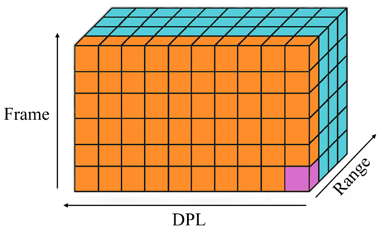Focusing on the range cell where the target resides (denoted $r_0$, as shown in the orange region of Figure 1), we extract M pulses and apply an F-point FFT along the slow-time dimension to obtain a single-frame Doppler-spectrum vector:

$${\mathbf{S}}_{\mathrm{Doppler}}\left(r_0\right)={\left\{{\displaystyle \sum _{m=1}^M}{\mathbf{S}}_{m,r_0}{e}^{-j2\pi {\displaystyle \frac{f-1}{F}}(m-1)}\right\}}_{f=1}^F\in {\mathbb{C}}^F.$$

(3)

The f-th Doppler channel corresponds to radial velocity $v_r$ via $f_d=2v_r/\lambda$, with $\lambda$ the wavelength. This transforms the pulse sequence into a frequency-domain representation of target motion within one CPI.

Stacking range–Doppler matrices from N consecutive CPIs produces a three-dimensional data cube $\mathbf{Q}\in {\mathbb{C}}^{R\times F\times N}$ (Figure 1). A target track segment is formed by extracting T contiguous frames from this cube ($T=N$ for one intercepted segment). Each frame is associated with radar-estimated kinematic parameters (azimuth, elevation, range, velocity).

Since the FFT output is complex-valued, it is converted to a real-valued Doppler representation before feeding into the network. In this work, the magnitude spectrum is adopted:

$${\mathbf{d}}_i=\left|{\mathbf{S}}_{\mathrm{Doppler}}\left(r_0\right)\right|\in {\mathbb{R}}^F.$$

(4)

To handle variable-length observations, a sliding-window strategy generates equal-length segments. After windowing, the Doppler-spectrum and kinematic data are organized as tensors [33]:

$$\mathbf{D}\in {\mathbb{R}}^{B\times T\times F},\mathbf{P}\in {\mathbb{R}}^{B\times T\times Z},$$

(5)

where B is the batch size, T the number of frames, F the Doppler channels and Z the kinematic parameters per frame. Both are normalized to $[0,1]$ via min–max scaling [34]:

$${\mathbf{D}}_{\mathrm{norm}}={\displaystyle \frac{\mathbf{D}-min\left(\mathbf{D}\right)}{max\left(\mathbf{D}\right)-min\left(\mathbf{D}\right)}},{\mathbf{P}}_{\mathrm{norm}}={\displaystyle \frac{\mathbf{P}-min\left(\mathbf{P}\right)}{max\left(\mathbf{P}\right)-min\left(\mathbf{P}\right)}}.$$

(6)

The pair $({\mathbf{D}}_{\mathrm{norm}},{\mathbf{P}}_{\mathrm{norm}})$ constitutes the unified sequence representation, with high-dimensional Doppler responses and low-dimensional kinematic states, and serves as input to graph construction.

3.3. Frame-Level Graph Construction

A radar observation sequence is modelled as a graph $\mathcal{G}=(\mathcal{V},\mathcal{E})$, where each node $v_i\in \mathcal{V}$ corresponds to one observation frame, not a feature dimension or sensor station [31]. This matches the sequence-level classification goal: the target category must be inferred from the evolution of frame-level observations.

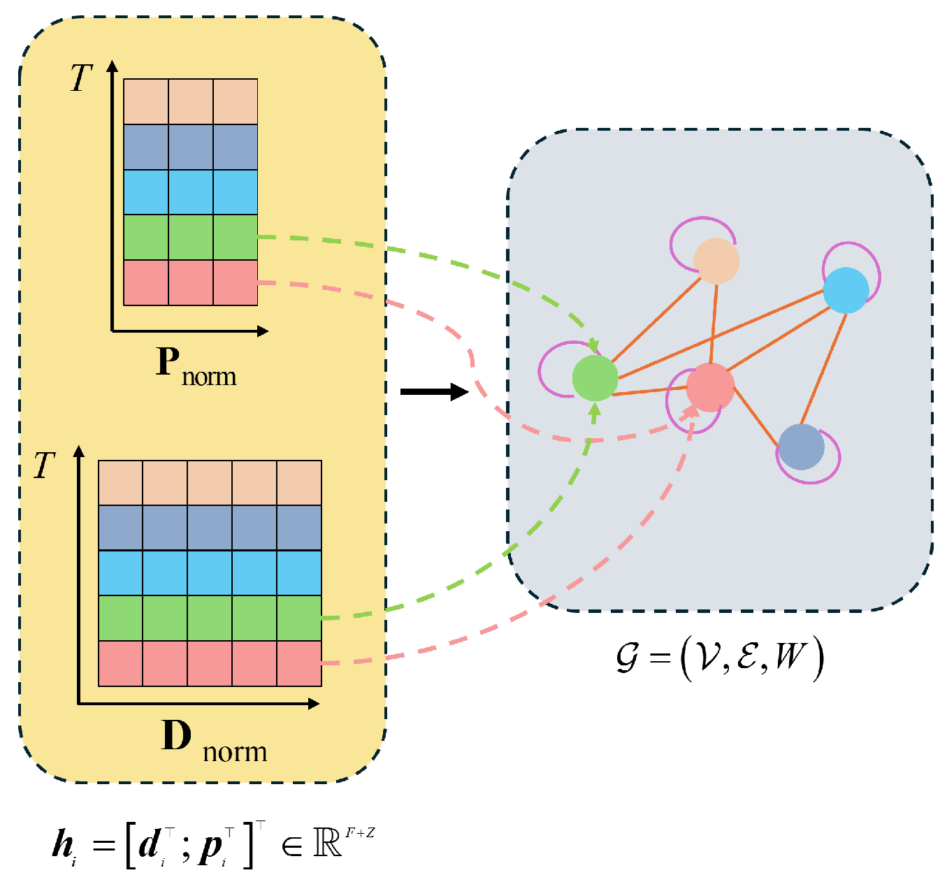
For node i, the feature vector concatenates the Doppler and kinematic vectors observed at the same time step:

$${\mathbf{h}}_i={[{\mathbf{d}}_i^{\top };{\mathbf{p}}_i^{\top }]}^{\top }\in {\mathbb{R}}^{F+Z}.$$

(7)

Although this defines the complete node attribute, the proposed model processes the two feature groups in separate streams before adaptive fusion to preserve heterogeneity.

Edges encode local temporal adjacency. With a temporal window size $\tau$, an edge connects nodes i and j if $0<|i-j|\le \tau$, forming the edge set ${\mathcal{E}}_{\mathrm{time}}$. Self-loops are added to retain each node’s own information. The adjacency matrix $\mathbf{A}\in {\{0,1\}}^{T\times T}$ is binary:

$${\mathbf{A}}_{ij}=\left\{\begin{array}{cc}1,\hfill & \mathrm{if}(i,j)\in {\mathcal{E}}_{\mathrm{time}}\mathrm{or}i=j,\hfill \\ 0,\hfill & \mathrm{otherwise}.\hfill \end{array}\right.$$

(8)

The resulting graph is a frame-level spatio-temporal representation: node attributes capture heterogeneous radar measurements, and edges impose local temporal dependencies. Figure 2 illustrates node composition, and Figure 3 shows the edge construction for $T=7$, $\tau =2$.

This formulation offers two advantages for model design: (i) it explicitly preserves the one-to-one frame–node correspondence, making the temporal topology explicit, and (ii) it provides a natural structure for combining global temporal modelling with local neighborhood aggregation in DS-STCAGCN.

4. Proposed DS-STCAGCN

4.1. Overall Architecture

DS-STCAGCN is a dual-stream spatio-temporal graph learning framework for radar target classification. “Spatio-temporal” refers to graph-topological relationships among temporally ordered nodes, not geographic coordinates. The input is a continuous single-radar observation sequence where each time step contains a Doppler-spectrum vector and a radar-estimated kinematic vector.

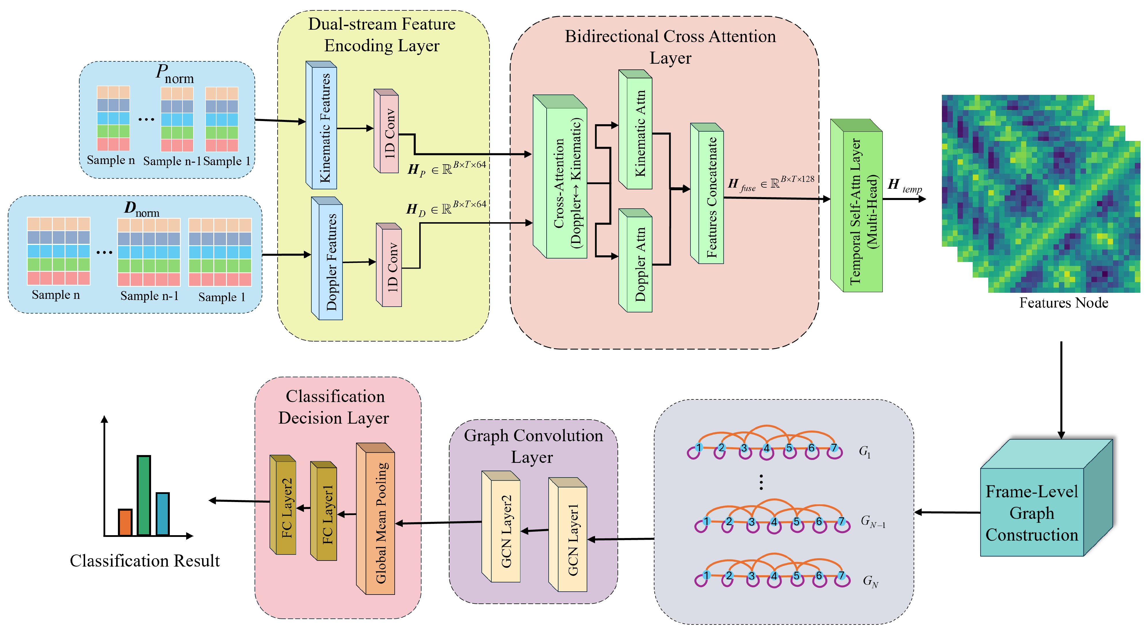
As described in Section 3, each target segment is first represented as a frame-level graph with temporal adjacency edges. On this graph, DS-STCAGCN performs structured sequence modelling through five components (Figure 4): (1) dual-stream heterogeneous feature encoding, (2) bidirectional cross-attention fusion, (3) temporal attention, (4) graph convolution, and (5) a classification head.

Let the normalized inputs be ${\mathbf{D}}_{\mathrm{norm}}\in {\mathbb{R}}^{B\times T\times F}$ and ${\mathbf{P}}_{\mathrm{norm}}\in {\mathbb{R}}^{B\times T\times Z}$ (batch size B, frames T, Doppler dimension F, kinematic dimension Z). The overall pipeline is

$${\mathbf{D}}_{\mathrm{norm}},{\mathbf{P}}_{\mathrm{norm}}\to {\mathbf{H}}_D,{\mathbf{H}}_P\to {\mathbf{H}}_{\mathrm{fuse}}\to {\mathbf{H}}_{\mathrm{temp}}\to {\mathbf{H}}_{\mathrm{GCN}}\to {\mathbf{y}}_{\mathrm{pred}},$$

(9)

where ${\mathbf{H}}_D$ and ${\mathbf{H}}_P$ are latent Doppler and kinematic representations, ${\mathbf{H}}_{\mathrm{fuse}}$ is the cross-attention fusion, ${\mathbf{H}}_{\mathrm{temp}}$ is the temporally enhanced feature, ${\mathbf{H}}_{\mathrm{GCN}}$ denotes graph-convolved node features, and ${\mathbf{y}}_{\mathrm{pred}}$ is the predicted class probability.

Instead of early concatenation, DS-STCAGCN preserves modality heterogeneity via separate encoding, then progressively integrates features through cross-attention, temporal modelling, and local graph aggregation. This aligns with the nature of radar tracks: the two feature groups are complementary but statistically different, and both global evolution and local frame correlations are informative for sequence-level classification.

4.2. Dual-Stream Heterogeneous Feature Encoding

Doppler-spectrum and kinematic features are complementary but heterogeneous: high-dimensional spectral responses vs. low-dimensional motion states. Direct concatenation may suppress modality-specific structures. Therefore, ${\mathbf{D}}_{\mathrm{norm}}$ and ${\mathbf{P}}_{\mathrm{norm}}$ are first encoded in two separate streams, both projecting to a 64-dimensional latent space. We implement each encoder as a one-dimensional convolution (Conv1D), which captures local temporal patterns while preserving the frame-wise correspondence required by the subsequent graph construction [35]:

$${\mathbf{H}}_D=\mathrm{ReLU}\left({\mathrm{Conv}1\mathrm{D}}_{64}\left({\mathbf{D}}_{\mathrm{norm}}\right)\right)\in {\mathbb{R}}^{B\times T\times 64},$$

(10)

$${\mathbf{H}}_P=\mathrm{ReLU}\left({\mathrm{Conv}1\mathrm{D}}_{64}\left({\mathbf{P}}_{\mathrm{norm}}\right)\right)\in {\mathbb{R}}^{B\times T\times 64}.$$

(11)

Separate encoders prevent premature blending of heterogeneous descriptors, while the shared latent dimension facilitates subsequent cross-stream interaction [36].

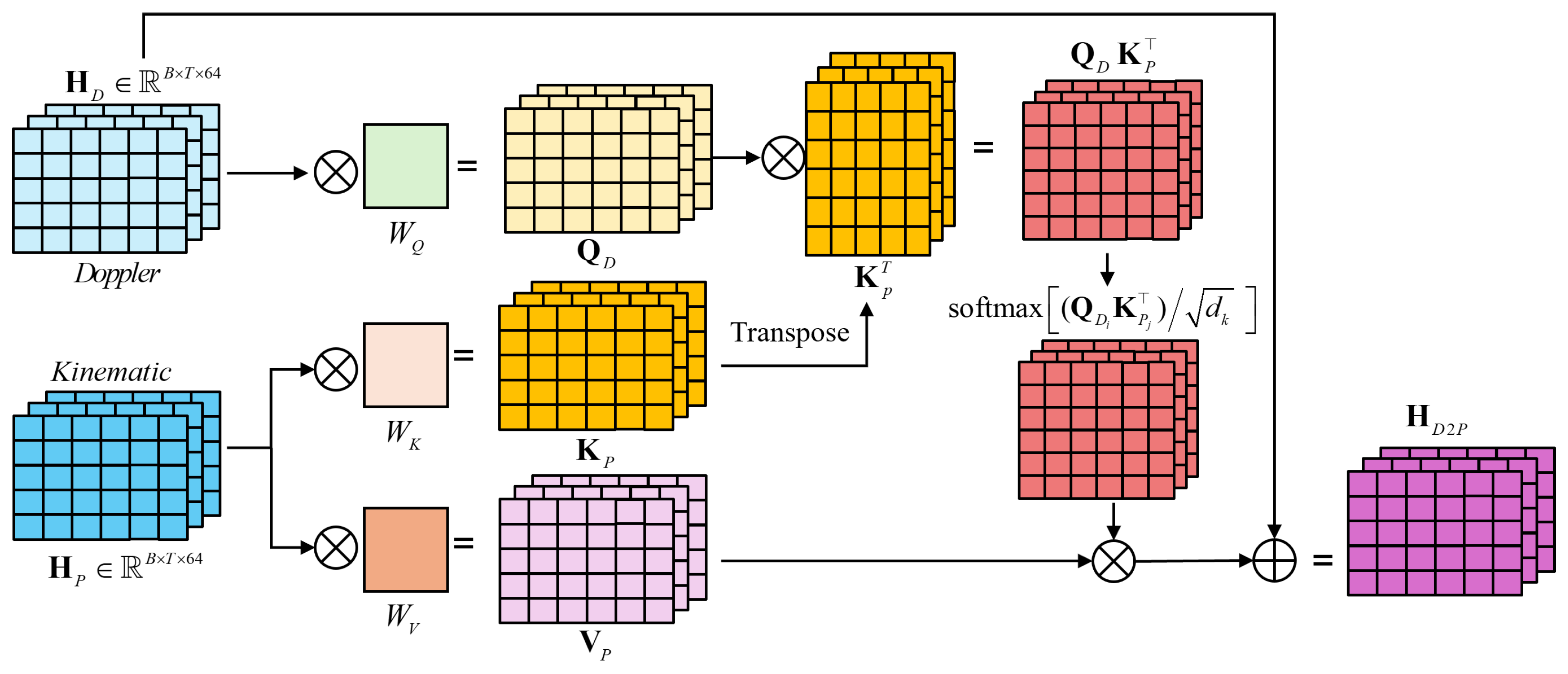
4.3. Bidirectional Cross-Attention Fusion

Cross-attention adaptively exchanges information between the two streams [37]. Let source $src\in \{D,P\}$ and target $tgt\in \{P,D\}$ with $src\ne tgt$. Learnable projection matrices ${\mathbf{W}}_Q^{src},{\mathbf{W}}_K^{tgt},{\mathbf{W}}_V^{tgt}\in {\mathbb{R}}^{64\times d_k}$ (with $d_k=64$) map the respective features to query, key, and value spaces:

$$\begin{array}{cc}\hfill {\mathbf{Q}}^{src}& ={\mathbf{H}}_{src}{\mathbf{W}}_Q^{src},\hfill \end{array}$$

(12)

$$\begin{array}{cc}\hfill {\mathbf{K}}^{tgt}& ={\mathbf{H}}_{tgt}{\mathbf{W}}_K^{tgt},\hfill \end{array}$$

(13)

$$\begin{array}{cc}\hfill {\mathbf{V}}^{tgt}& ={\mathbf{H}}_{tgt}{\mathbf{W}}_V^{tgt}.\hfill \end{array}$$

(14)

The cross-attention weight between source time step i and target time step j is

$${\alpha }_{ij}^{src\to tgt}=\mathrm{softmax}\left({\displaystyle \frac{{\mathbf{Q}}_i^{src}{\left({\mathbf{K}}_j^{tgt}\right)}^{\top }}{\sqrt{d_k}}}\right),$$

(15)

and the output for time step i combines target values with a residual connection:

$${\mathbf{H}}_i^{src\to tgt}=\sum _j{\alpha }_{ij}^{src\to tgt}{\mathbf{V}}_j^{tgt}+{\mathbf{H}}_i^{src}.$$

(16)

Bidirectional attention is performed in two directions:

• $D\to P$: Doppler queries kinematic features, yielding ${\mathbf{H}}_{D2P}={\mathbf{H}}^{D\to P}$.
• $P\to D$: Kinematic queries Doppler features, yielding ${\mathbf{H}}_{P2D}={\mathbf{H}}^{P\to D}$.

Both directions are concatenated channel-wise to form the fused representation

$${\mathbf{H}}_{\mathrm{fuse}}=[{\mathbf{H}}_{D2P}\Vert {\mathbf{H}}_{P2D}]\in {\mathbb{R}}^{B\times T\times 128}.$$

(17)

A schematic illustration of the Doppler-to-kinematic cross-attention is provided in Figure 5. The definitions of all cross-attention variables are listed in

Table 1. Definitions of variables in bidirectional cross-attention.

Variable	Definition
${\mathbf{H}}_{D_i}$, ${\mathbf{H}}_{D_j}$	Doppler-spectrum latent features at time steps i and j.
${\mathbf{H}}_{P_i}$, ${\mathbf{H}}_{P_j}$	Kinematic latent features at time steps i and j.
${\mathbf{W}}_Q^{src},{\mathbf{W}}_K^{tgt},{\mathbf{W}}_V^{tgt}$	Projection matrices for source $src$ and target $tgt$; dimensions $64\times d_k$. For $D\to P$: $(src,tgt)=(D,P)$; for $P\to D$: $(src,tgt)=(P,D)$.
${\mathbf{Q}}^{src},{\mathbf{K}}^{tgt},{\mathbf{V}}^{tgt}$	Query, key, value matrices from linear projections.
${\mathbf{Q}}_i^{src},{\mathbf{K}}_j^{tgt},{\mathbf{V}}_j^{tgt}$	Time-step slices of the above matrices.
$d_k$	Scaling dimension, set to 64.
${\alpha }_{ij}^{src\to tgt}$	Attention weight: dependency of source step i on target step j.
${\mathbf{H}}_{D2P}$, ${\mathbf{H}}_{P2D}$	Outputs of $D\to P$ and $P\to D$ cross-attention, each with residual addition.

. This bidirectional design ensures that each stream can exploit complementary cues from the other before temporal modelling.

4.4. Temporal Attention and Graph Convolution

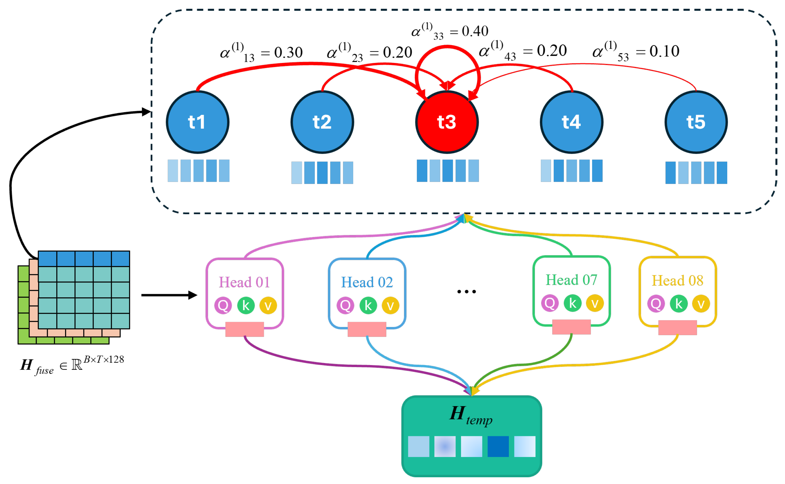
The fused feature ${\mathbf{H}}_{\mathrm{fuse}}$ still lacks explicit long-range temporal dependencies and local neighborhood aggregation. DS-STCAGCN therefore applies multi-head self-attention followed by graph convolution.

Temporal attention. ${\mathbf{H}}_{\mathrm{fuse}}$ is processed by an h = 8 head self-attention. The feature is split into h subspaces of dimension d_head = 16. For head k, projections ${\mathbf{W}}_Q^{\left(k\right)},{\mathbf{W}}_K^{\left(k\right)},{\mathbf{W}}_V^{\left(k\right)}\in {\mathbb{R}}^{16\times 16}$ produce

$$\begin{array}{c}\hfill {\mathbf{Q}}_k={\mathbf{H}}_{\mathrm{head},k}{\mathbf{W}}_Q^{\left(k\right)},{\mathbf{K}}_k={\mathbf{H}}_{\mathrm{head},k}{\mathbf{W}}_K^{\left(k\right)},{\mathbf{V}}_k={\mathbf{H}}_{\mathrm{head},k}{\mathbf{W}}_V^{\left(k\right)}.\end{array}$$

(18)

Attention weights and head outputs are

$${\alpha }_{ij}^{\left(k\right)}=\mathrm{softmax}\left({\displaystyle \frac{{\mathbf{Q}}_{k,i}{\mathbf{K}}_{k,j}^{\top }}{\sqrt{d_{\mathrm{head}}}}}\right),{\mathbf{H}}_{\mathrm{attn},k}={\displaystyle \sum _{j=1}^T}{\alpha }_{ij}^{\left(k\right)}{\mathbf{V}}_{k,j}.$$

(19)

The concatenated heads are projected back to 128 dimensions:

$${\mathbf{H}}_{\mathrm{temp}}=\mathrm{Concat}({\mathbf{H}}_{\mathrm{attn},1},\dots ,{\mathbf{H}}_{\mathrm{attn},8}){\mathbf{W}}_O\in {\mathbb{R}}^{B\times T\times 128}.$$

(20)

Figure 6 depicts the temporal attention mechanism.

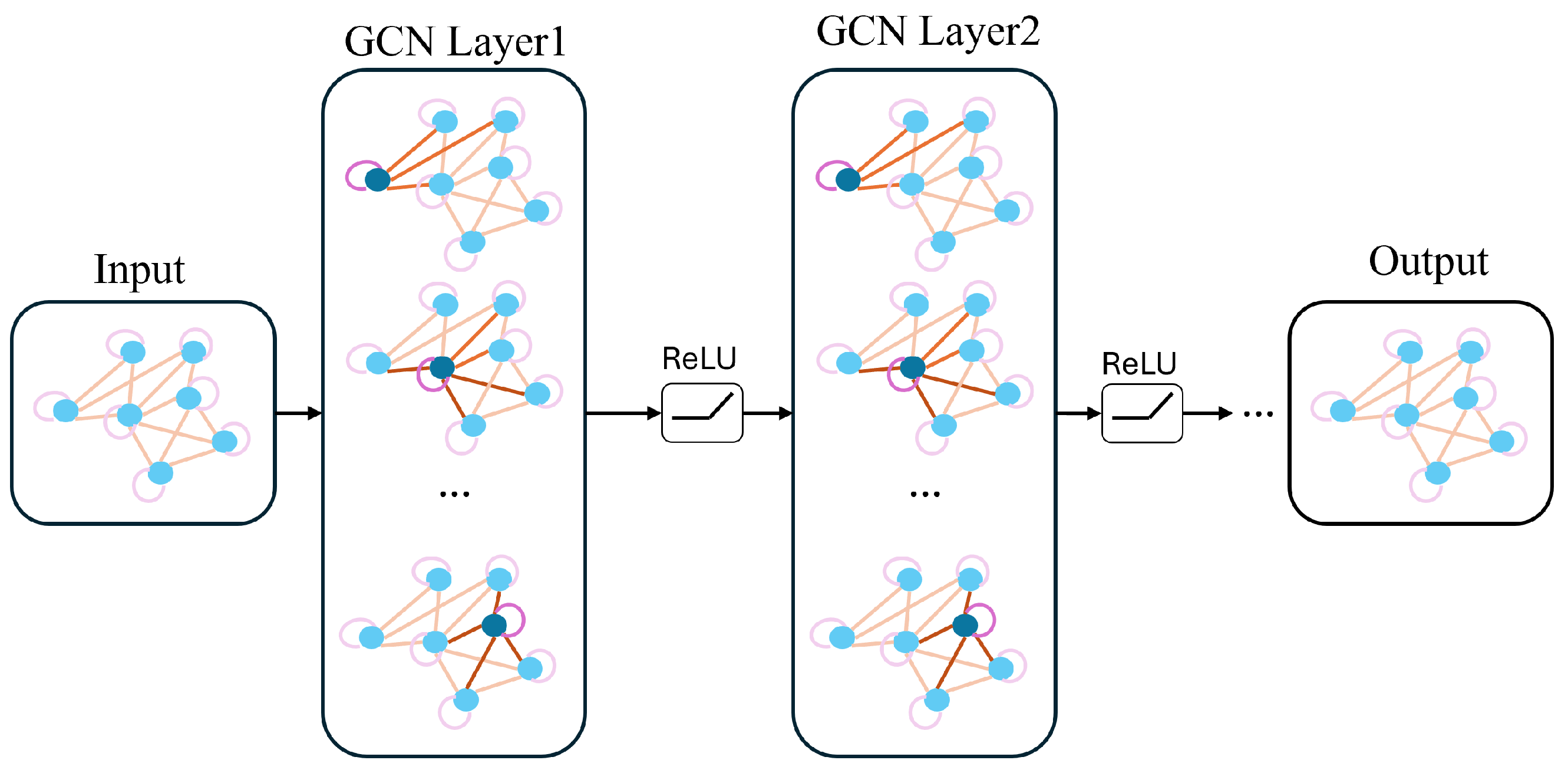
Graph convolution. Temporal self-attention captures global dependencies but not the explicit local topology [38]. The structure of the graph convolution layers is shown in Figure 7. We apply two GCNConv layers (edge weights fixed to 1, using adjacency $\mathbf{A}$ from Equation (8)) to aggregate local neighborhood information [39]:

$$\begin{array}{cc}\hfill {\mathbf{H}}_{\mathrm{GCN}1}& =\mathrm{ReLU}\left({\mathrm{GCNConv}}_{128\to 128}({\mathbf{H}}_{\mathrm{temp}},\mathbf{A})\right)\in {\mathbb{R}}^{B\times T\times 128},\hfill \end{array}$$

(21)

$$\begin{array}{cc}\hfill {\mathbf{H}}_{\mathrm{GCN}2}& =\mathrm{ReLU}\left({\mathrm{GCNConv}}_{128\to 64}({\mathbf{H}}_{\mathrm{GCN}1},\mathbf{A})\right)\in {\mathbb{R}}^{B\times T\times 64}.\hfill \end{array}$$

(22)

Temporal attention and graph convolution are complementary: the former models global contextual dependencies, while the latter enforces local temporal continuity. Together they encode both long-range and neighborhood structures. We adopt GCN instead of more complex models such as GAT because the graph topology constructed in this paper features a deterministic temporal adjacency structure without implicit edge weights. The standard GCN can efficiently aggregate local temporal neighborhood information. In contrast, complex models like GAT require additional parameters to learn edge weights and are suitable for scenarios where the importance of edges is unknown. Employing such models will only unnecessarily increase computational complexity and lead to overfitting.

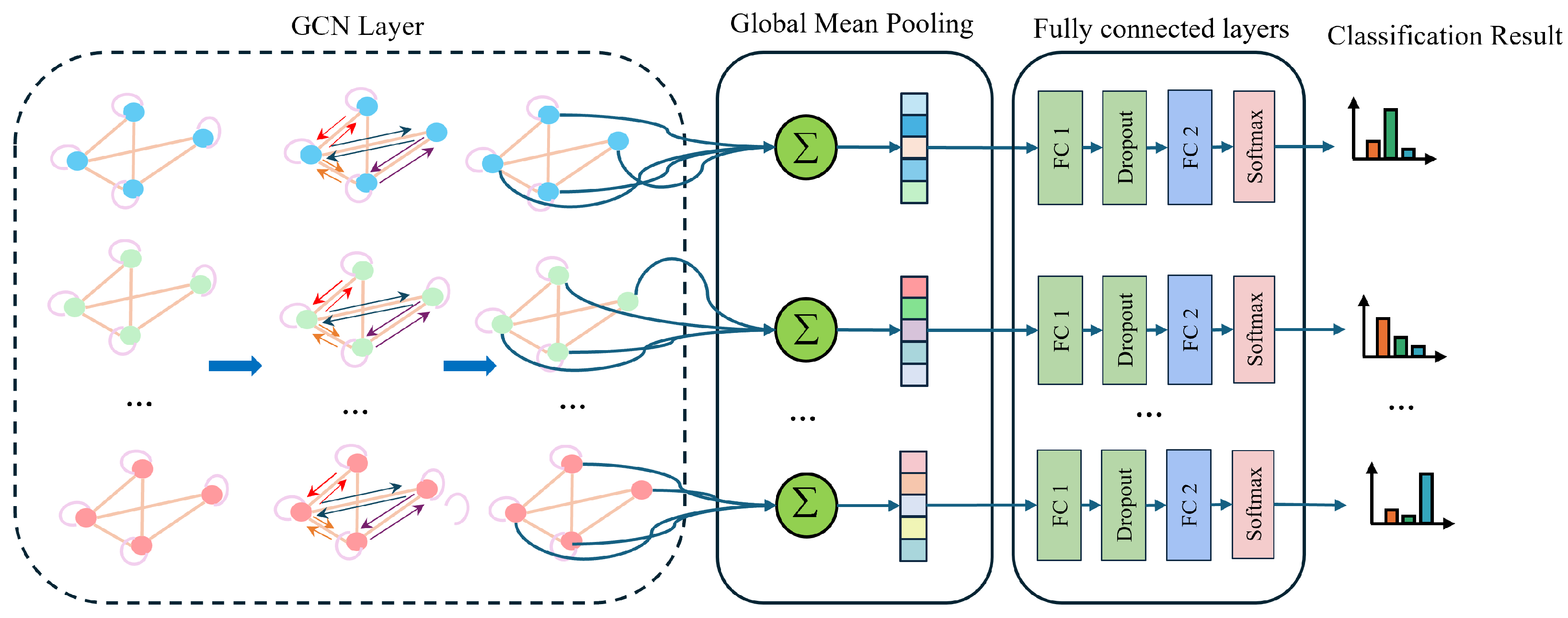
4.5. Classification Head and Training Objective

To obtain a graph-level representation, global average pooling is applied over the time steps of ${\mathbf{H}}_{\mathrm{GCN}2}$ [40]:

$${\mathbf{h}}_{\mathrm{global}}={\displaystyle \frac{1}{T}}{\displaystyle \sum _{t=1}^T}{\mathbf{H}}_{\mathrm{GCN}2}^{\left(t\right)}\in {\mathbb{R}}^{B\times 64}.$$

(23)

A classifier head (two fully connected layers, ReLU, dropout) then produces class probabilities [41]:as illustrated in Figure 8

$${\mathbf{y}}_{\mathrm{pred}}=\mathrm{Softmax}\left({\mathrm{FC}}_{64\to 32\to C}\left({\mathbf{h}}_{\mathrm{global}}\right)\right).$$

(24)

The model is trained end-to-end by minimizing the cross-entropy loss between predicted probabilities ${\mathbf{y}}_{\mathrm{pred}}$ and one-hot labels $\mathbf{y}$ [41]:

$${\mathcal{L}}_{\mathrm{CE}}=-{\displaystyle \frac{1}{B}}{\displaystyle \sum _{b=1}^B}{\displaystyle \sum _{c=1}^C}{y}_{b,c}log\left(y_{\mathrm{pred},b,c}\right).$$

(25)

5. Datasets and Experimental Settings

5.1. LSS-DAUR-1.0 Digital-Array Radar Dataset

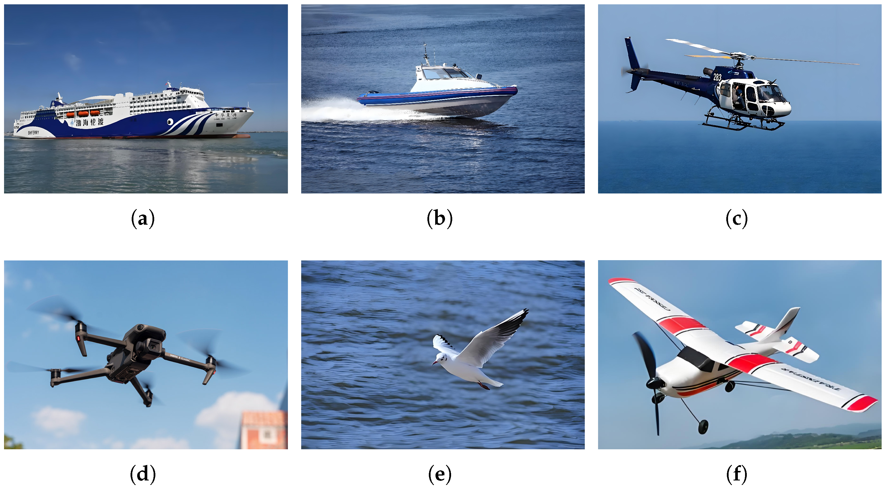
LSS-DAUR-1.0 contains continuous observation sequences of six classes: passenger ship, speedboat, helicopter, rotor drone, bird, and fixed-wing drone, as shown in Figure 9. Each sample provides time-aligned Doppler-spectrum information and four kinematic parameters (azimuth, elevation, range, velocity). Therefore, this dataset is consistent with the problems to be addressed in this study. Targets were confirmed by visual or optoelectronic means.

Table 2. Parameters of the digital array radar.

Radar Parameter	Value
Carrier Frequency (GHz)	1.36
Bandwidth (MHz)	4
Transmit Power (W)	400
Pulse Repetition Frequency (kHz)	5
Pulse Width (µs)	2
Velocity Resolution (m/s)	0.1346
Range Resolution (m)	30
Doppler channel number	512

lists the main radar parameters. Representative feature characteristics are summarized in

Table 3. Summary of multi-dimensional target features.

Target Type	Avg. Doppler Shift (Hz)	Signal Energy (dB)	Trajectory Characteristics
Passenger ship	Low	High	Straight, fixed routes
Speedboat	High	Medium	Long, high-speed
Helicopter	High	High	Small-angle turns, comb-like DWD
Rotor drone	Medium	Low	No pronounced micro-Doppler
Bird	Low	Low	Random, sharp turns
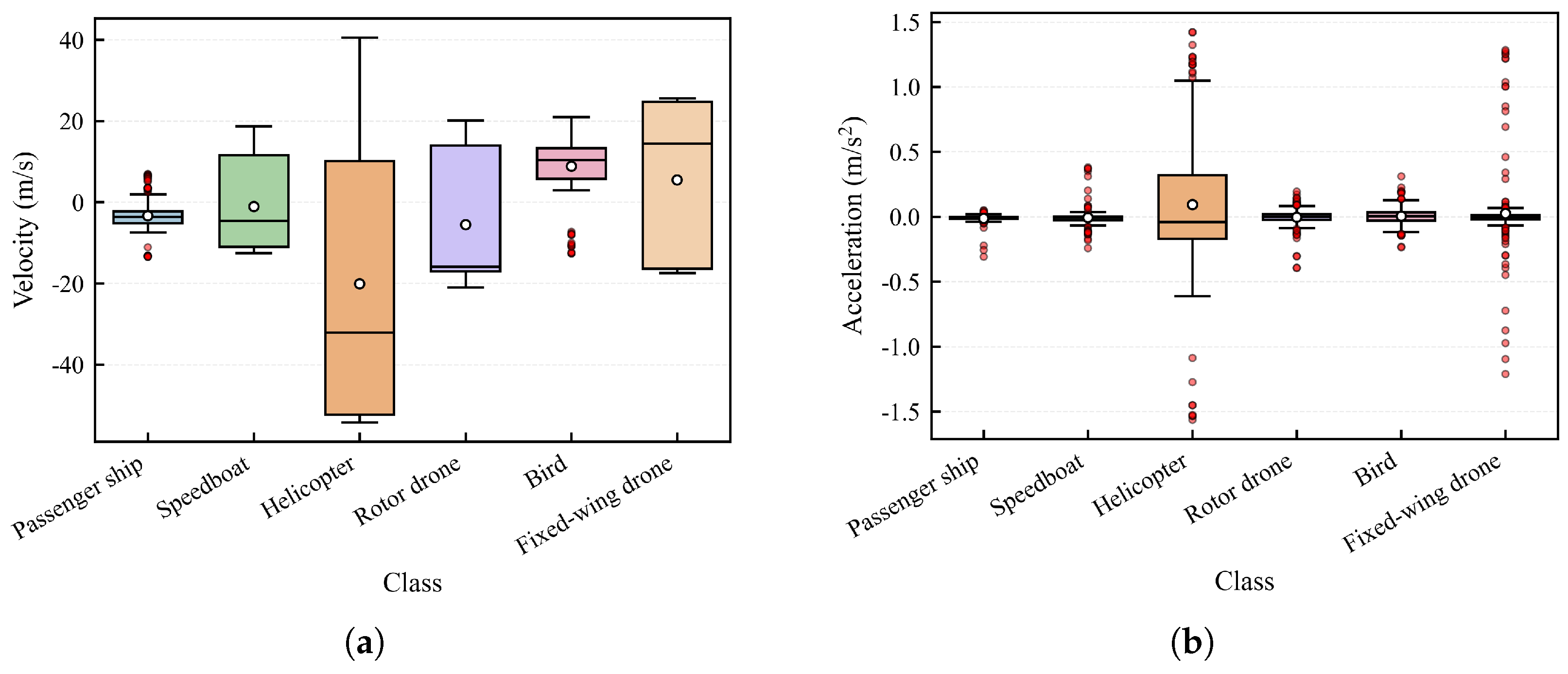
Fixed-wing drone	High	Medium	Diving, altitude changes

, and kinematic distributions are shown in Figure 10.

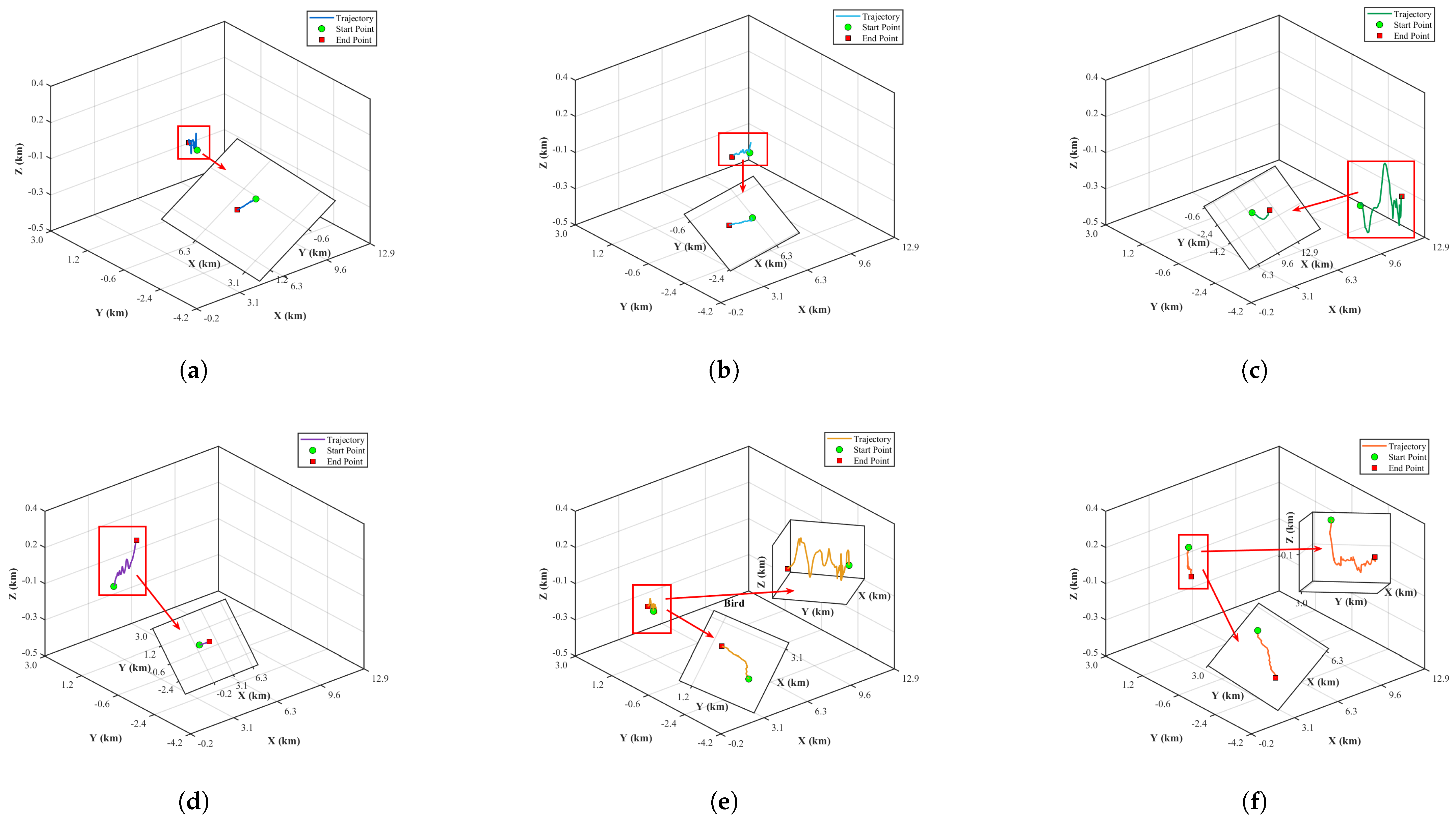
From the DWDs (Figure 11) and 3D tracks (Figure 12), target distinctions align with Table 3: Doppler shift and signal energy vary by target type (e.g., high shifts for speedboats/helicopters, low for ships/birds), while trajectory patterns range from stable routes (ships) to sharp turns (birds) and dives (fixed-wing drones); helicopters additionally exhibit comb-like DWD stripes.

These observations confirm that Doppler signatures and kinematic trajectories provide complementary discriminative information, motivating the dual-stream design of DS-STCAGCN.

To ensure consistent sequence modelling, a sliding window of length $T=30$ frames is applied to raw tracks [42]. To avoid data leakage from highly overlapped windows, a track-level split is adopted: the dataset is divided into training and validation sets at an 8:2 ratio with stratified sampling (seed = 42) at the track level [43]. Sliding-window segmentation is then performed independently within each split. The normalization statistics are computed from the training set only and applied to both splits.

Class-dependent step sizes are used during sliding-window augmentation to mitigate imbalance: passenger ship ($s=10$), speedboat ($s=5$), helicopter ($s=3$), rotor drone ($s=5$), bird ($s=10$), fixed-wing drone ($s=5$). Each graph sample comprises $T=30$ nodes, with Doppler-spectrum dimension $F=512$ and kinematic dimension $Z=4$ (azimuth, elevation, range, velocity). The temporal adjacency graph uses $\tau =3$ (Equation (8)). The sample distribution is given in

Table 4. Dataset partition.

Target Type	Total	Proportion	Training	Validation
Passenger ship	246	16.70%	197	49
Speedboat	231	15.68%	185	46
Helicopter	217	14.73%	174	43
Rotor drone	250	16.97%	200	50
Bird	237	16.09%	189	48
Fixed-wing drone	292	19.82%	233	59
Total	1473	100.00%	1178	295

.

5.2. LSS-PR-1.0 Passive-Radar Dataset

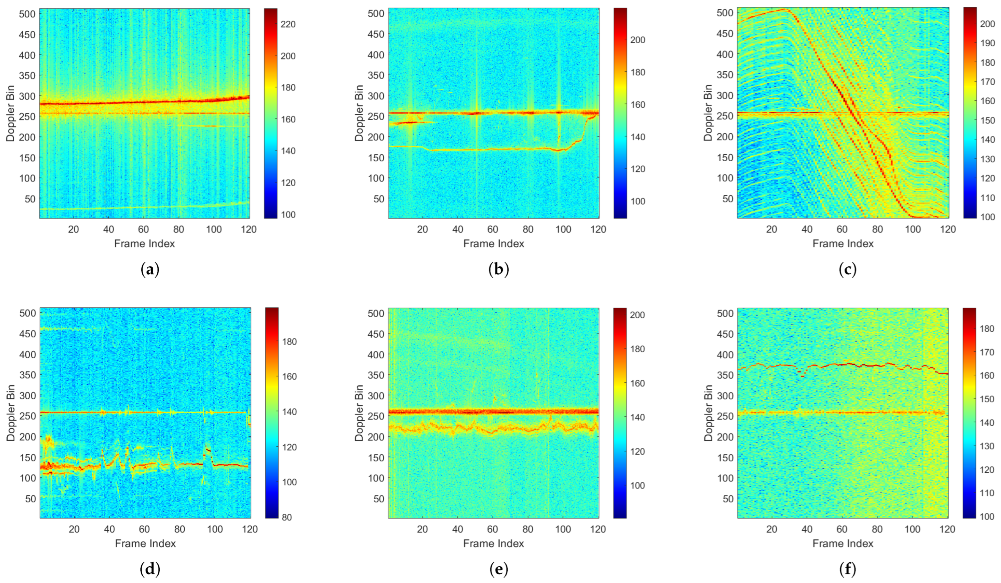
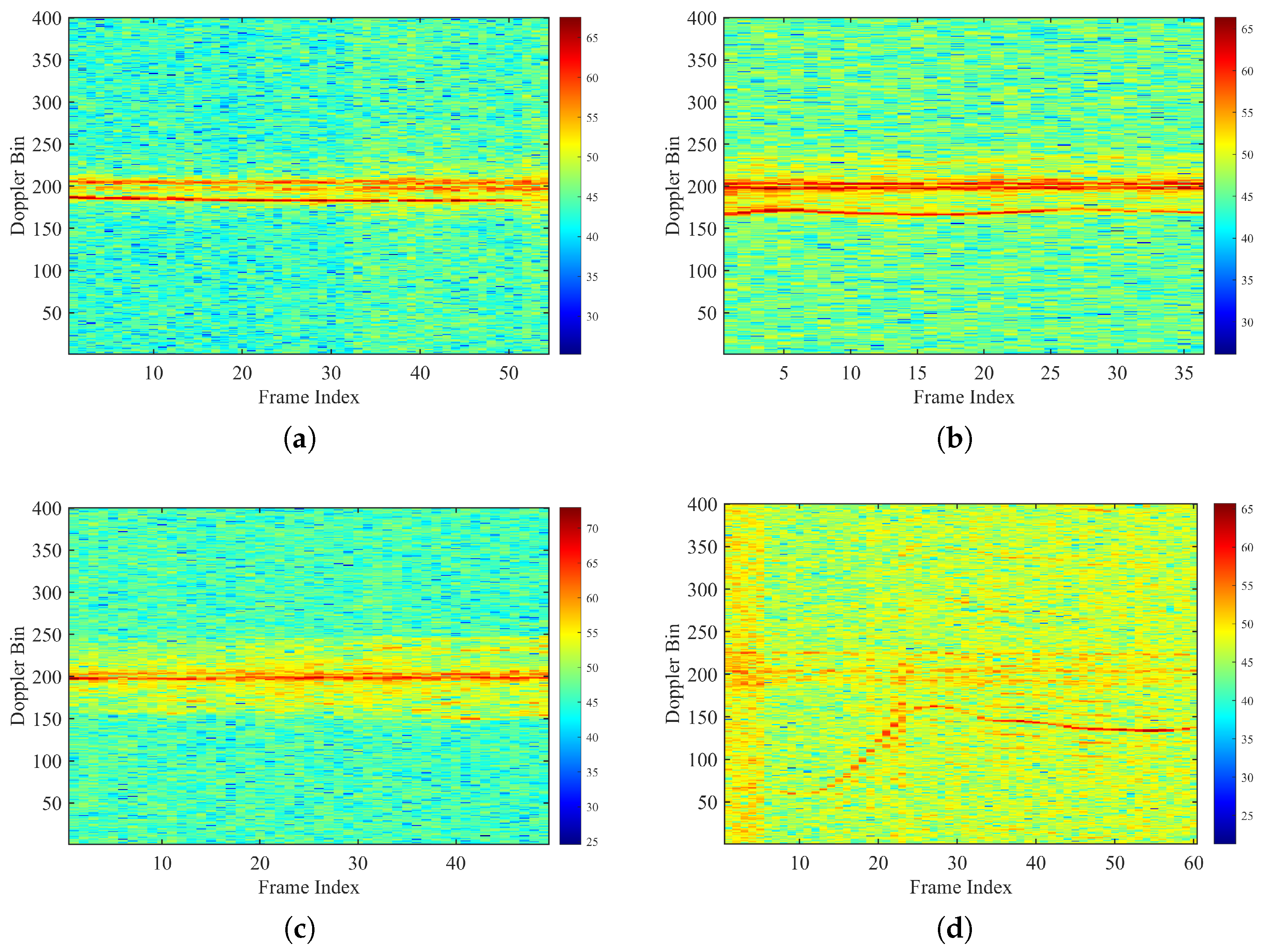
To further assess generalization, experiments are conducted on the public passive-radar dataset LSS-PR-1.0 [29]. This dataset was collected using a passive radar operating at 470–806 MHz with DTMB signals, providing a different modality from the active L-band radar of LSS-DAUR-1.0. It contains four classes: passenger ship, speedboat, rotor drone, and helicopter. Radar parameters are listed in

Table 5. Basic parameters of the passive radar for the LSS-PR-1.0 dataset.

Radar Parameter	Value
Receivable Frequency Range	470 MHz∼806 MHz
DTMB Signal Bandwidth	7.56 MHz
Range Resolution Unit	39.68 m
Azimuth Accuracy	1°
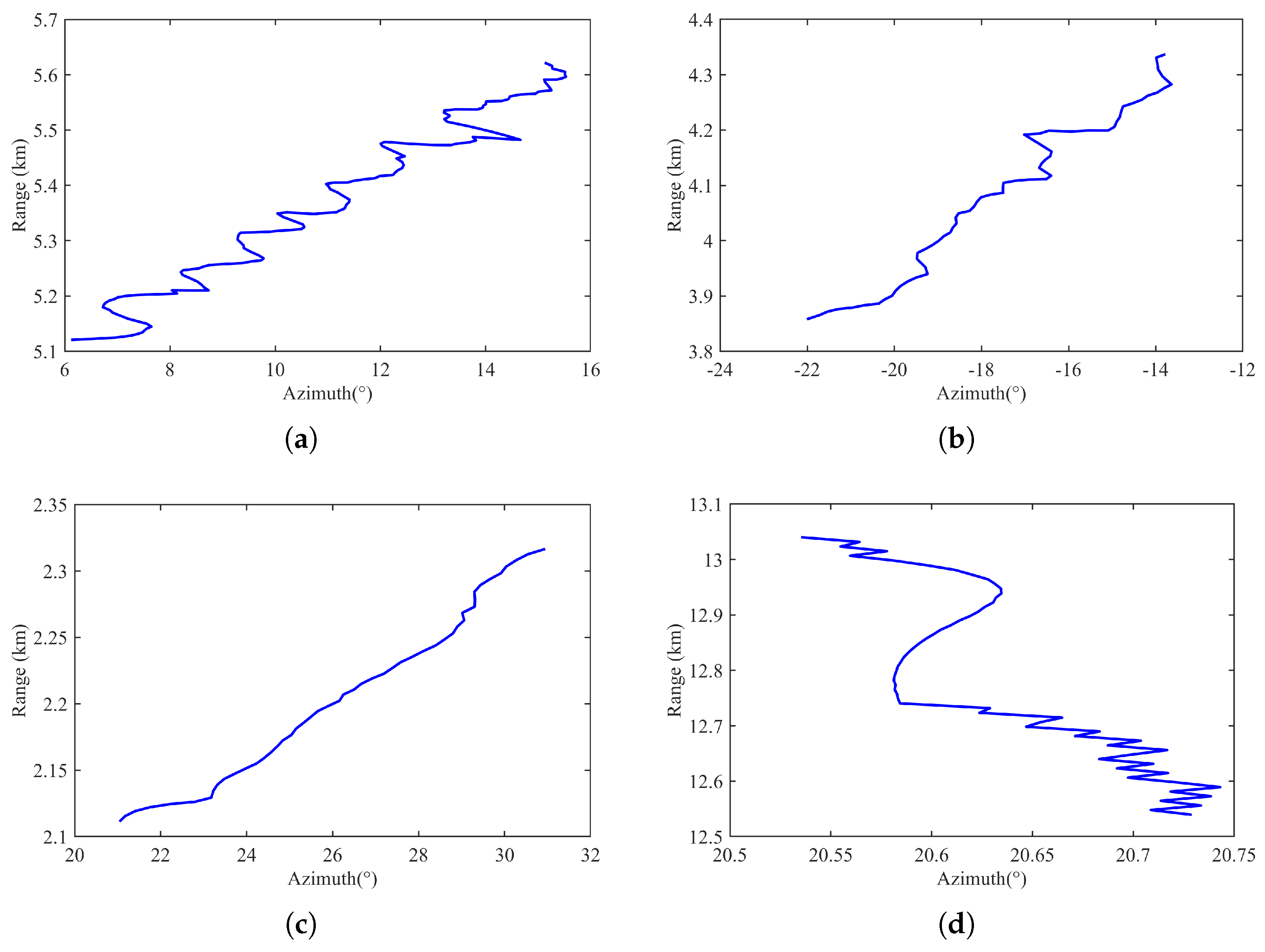
Data Update Cycle	1 s

, and representative DWDs and 2D trajectories are shown in Figure 13 and Figure 14. The same track-level split (8:2, seed 42), sliding-window ($T=30$), normalization, and graph construction ($\tau =3$) are applied. The resulting partition is shown in

Table 6. Dataset division of the LSS-PR-1.0 dataset.

Target Type	Total	Proportion	Training	Validation
Passenger ship	244	39.29%	195	49
Speedboat	121	19.48%	96	25
Rotor drone	78	12.56%	62	16
Helicopter	178	28.66%	142	36
Total	621	–	495	126

. The feature dimensions are $F=400$ and $Z=4$ (range, azimuth, horizontal velocity, vertical velocity), giving node dimension $F+Z=404$.

5.3. Implementation Details

Experiments are run on an NVIDIA RTX 4060 8G GPU with an Intel i7-12650H CPU, CUDA 11.8, PyTorch 2.4.1, and PyTorch Geometric 2.6.1 [44]. All models share the same train–validation split and environment. Training minimizes the cross-entropy loss (Equation (25)) using the AdamW optimizer [45] with dropout [46] and BatchNorm [47]. Common hyperparameters are listed in

Table 7. Training hyperparameter settings common to all models for fair comparison.

Parameter Name	Value
Optimizer	AdamW
Initial learning rate	$3\times {10}^{-4}$
L2 regularization factor	$\lambda =0.0005$
Dropout probability	0.5
Batch size	32
Maximum number of training epochs	100
Label smoothing epsilon	0.1

.

5.4. Evaluation Metrics and Compared Methods

We report accuracy, precision, recall, F1-score, support, macro average, weighted average, parameters (M), inference latency (IL, ms, batch size 1, averaged over 100 runs after warm-up), and throughput (FPS, batch size 32). Classification metrics are computed with scikit-learn [48]. Macro average treats classes equally; weighted average weights by class size.

Compared methods include three image-based models (ConvNeXt-Tiny, EfficientNetV2-S, CBAM-Swin-Transformer [16]) using 30-frame Doppler waterfall images; two sequence-based models (BiLSTM and an early-fusion Transformer Encoder) using Doppler-spectrum and kinematic sequences; and a handcrafted-feature fusion pipeline with XGBoost (v3.2.0) [49]. All deep models are trained and evaluated 10 times; mean accuracy and standard deviation are reported. The XGBoost baseline uses the same split. Noise robustness is evaluated under SNRs from $-10$ to 20 dB. Additive white Gaussian noise is injected into Doppler-spectrum data according to the target SNR, while kinematic parameters receive noise at 10% of the Doppler noise intensity. The SNR definition and noise construction are

$${\mathrm{SNR}}_{dB}=10{log}_{10}\left({\displaystyle \frac{P_{\mathrm{signal}}}{P_{\mathrm{noise}}}}\right)$$

(26)

$$\begin{array}{cc}\hfill P_{\mathrm{signal},\mathrm{Doppler}}& =\overline{{\left(\mathbf{D}\right)}^2},\hfill \\ \hfill {\mathrm{SNR}}_{\mathrm{linear}}& ={10}^{{\mathrm{SNR}}_{dB}/10},\hfill \\ \hfill P_{\mathrm{noise},\mathrm{Doppler}}& =P_{\mathrm{signal},\mathrm{Doppler}}/{\mathrm{SNR}}_{\mathrm{linear}},\hfill \\ \hfill {\mathbf{n}}_{\mathrm{Doppler}}& =\mathcal{N}(0,\sqrt{P_{\mathrm{noise},\mathrm{Doppler}}}),\hfill \\ \hfill {\mathbf{n}}_{\mathrm{kinematic}}& =\mathcal{N}(0,0.1·\sqrt{P_{\mathrm{noise},\mathrm{Doppler}}}).\hfill \end{array}$$

(27)

6. Experimental Results and Analysis

6.1. Overall Performance Comparison

Table 8. Comprehensive comparison of model classification performance and efficiency.

Model	Mean Acc (%)	Std(%)	Min (%)	Max (%)	Params (M)	IL@B1 (ms)	FPS@B32
DS-STCAGCN (Ours)	99.73	0.42	98.64	99.90	0.22	3.21	8810.70
ConvNeXt-Tiny	97.86	0.50	96.95	98.64	9.53	395.86	2.51
EfficientNetV2-S	97.39	0.92	96.27	99.32	6.96	406.98	2.47
CBAM-Swin-Transformer [16]	78.58	3.25	70.51	81.69	49.18	423.72	2.45
BiLSTM	87.32	2.11	84.07	90.51	3.23	2.69	13,550.09
Transformer Encoder	92.31	1.60	89.49	94.58	1.27	1.30	15,950.39
Handcrafted Feature Fusion + XGBoost	77.22	2.18	74.58	81.36	–	0.45	44,992.92

Note: Bold values indicate the best performance in each column. For Mean Acc, Min, Max, and FPS, higher is better. For Std, Params, and IL, lower is better. IL and FPS are measured end-to-end including data loading and all preprocessing steps (e.g., DWD image generation for image-based models via MATLAB (R2024a) plotting, tensor normalization for others). The XGBoost baseline is evaluated on CPU; all deep models are evaluated on an RTX 4060 GPU.

compares DS-STCAGCN with baseline methods on LSS-DAUR-1.0 over 10 independent runs.

DS-STCAGCN achieves the highest mean accuracy (99.73%) and the lowest standard deviation (0.42%). It improves mean accuracy by 1.87% and 2.34% over ConvNeXt-Tiny and EfficientNetV2-S, respectively, and maintains a minimum accuracy of 98.64%, demonstrating stable performance across runs.

With only 0.22 M parameters, DS-STCAGCN is more compact than all deep-learning baselines, yet outperforms larger image-based models. The sequence-based BiLSTM and Transformer Encoder have fewer parameters but substantially lower accuracy.

In inference efficiency, DS-STCAGCN yields 3.21 ms end-to-end latency and 8810.70 FPS throughput, both including data preprocessing. The image-based models suffer from much higher latency and drastically lower throughput due to the unavoidable overhead of Doppler waterfall image generation (391.3 ms per image). Consequently, DS-STCAGCN achieves over 100× lower latency and 3500× higher throughput than the image-based baselines, highlighting a critical practical advantage: by operating directly on radar feature tensors rather than rendered spectrograms, it eliminates the image-generation bottleneck and is far more suitable for real-time radar target recognition.

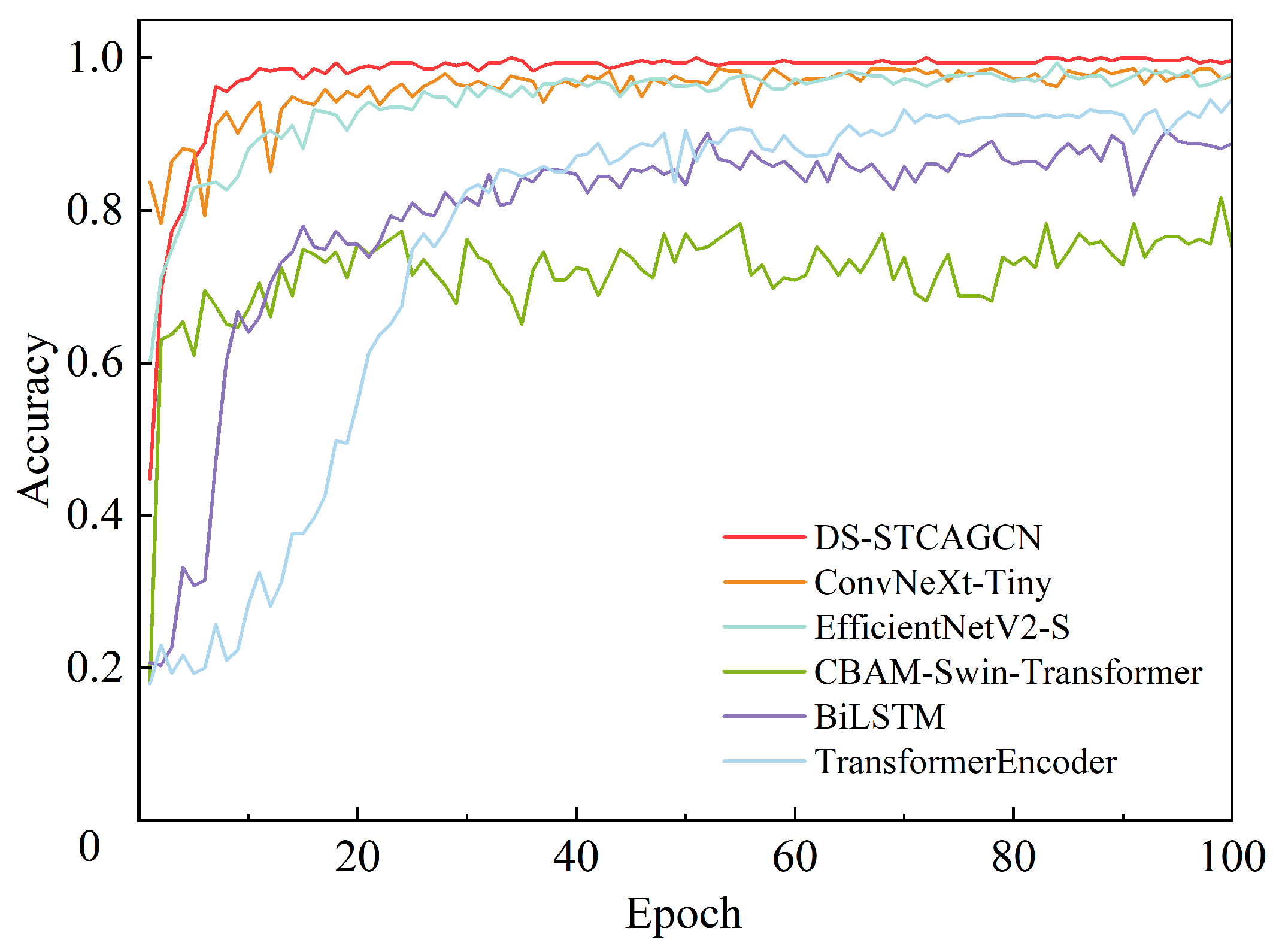
The Transformer Encoder and XGBoost achieve higher throughput, but their accuracies are substantially lower. Overall, DS-STCAGCN offers the best accuracy–efficiency balance. The validation curves in Figure 15 confirm its stable convergence.

6.2. Feature Discriminability Visualization

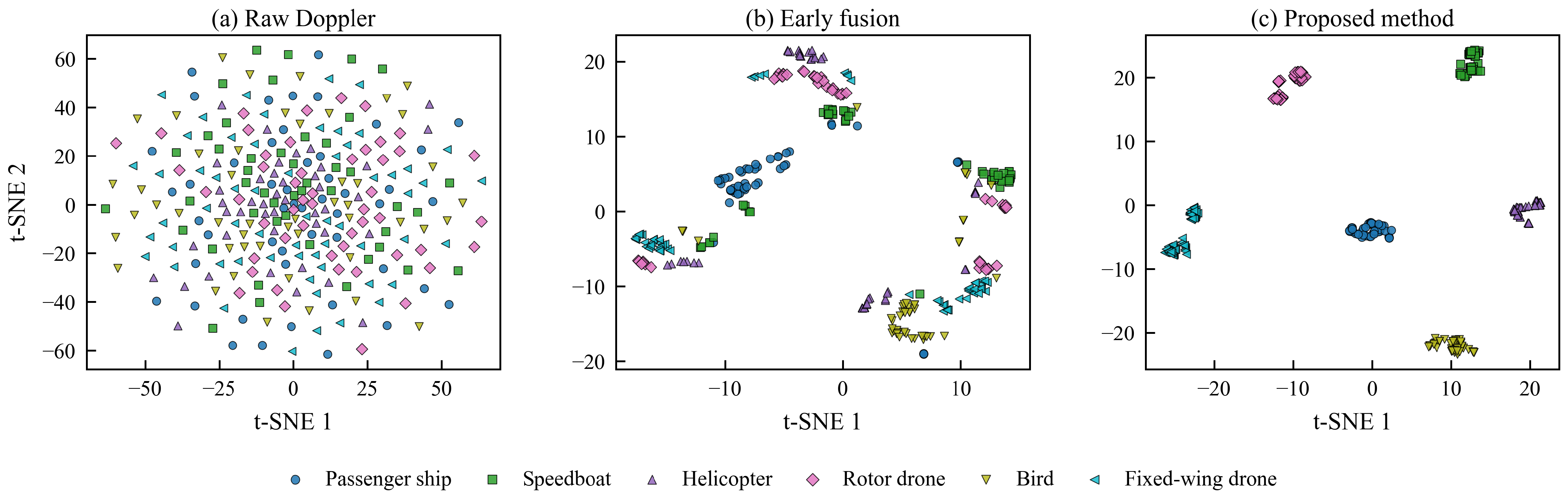
t-SNE visualizations of raw Doppler, early-fusion, and DS-STCAGCN features are shown in Figure 16. The raw Doppler features exhibit severe class overlap. Early fusion improves local cohesion but leaves partial mixing. DS-STCAGCN produces compact intra-class clusters and clear inter-class separation, confirming that the dual-stream, cross-attention, and graph convolution modules collectively enhance discriminability. These visual trends align with the quantitative gains in Table 8.

6.3. Ablation Study

To isolate the contribution of each component, ablation experiments are conducted under a fixed random seed, and the best validation accuracy of each variant is reported in

Table 9. Ablation study of the proposed DS-STCAGCN.

Variant	Doppler	Kinematic	Cross-Attn	Temporal Attn	GCN	Best Acc (%)	Best F1-Score
Full	✓	✓	Bi-dir	✓	✓	99.90	0.9989
w/o kinematic	✓	–	–	✓	✓	96.95	0.9695
D → P only	✓	✓	Uni-dir	✓	✓	98.98	0.9894
P → D only	✓	✓	Uni-dir	✓	✓	98.64	0.9865
w/o cross-attn	✓	✓	–	✓	✓	97.63	0.9764
w/o temporal attn	✓	✓	✓	–	✓	98.31	0.9831
w/o GCN	✓	✓	✓	✓	–	96.61	0.9662
w/o temporal attn & GCN	✓	✓	✓	–	–	92.54	0.9252

Note: ✓ indicates that the corresponding module is included in the variant. “Bi-dir” denotes bidirectional cross-attention, and “Uni-dir” denotes unidirectional cross-attention.

. The full model attains 99.90% accuracy and 0.9989 F1-score under this setting.

Removing the kinematic stream drops accuracy to 96.95%, confirming the value of kinematic data. Single-direction cross-attention (D → P: 98.98%, P → D: 98.64%) underperforms bidirectional fusion (99.90%), and removing cross-attention entirely lowers accuracy to 97.63%. Excluding temporal attention or GCN reduces accuracy to 98.31% and 96.61%, respectively; removing both yields 92.54%, demonstrating their complementary roles. These results are consistent with the t-SNE visualizations and confirm that each module contributes to the final representation quality.

6.4. Cross-Attention Interpretability Analysis

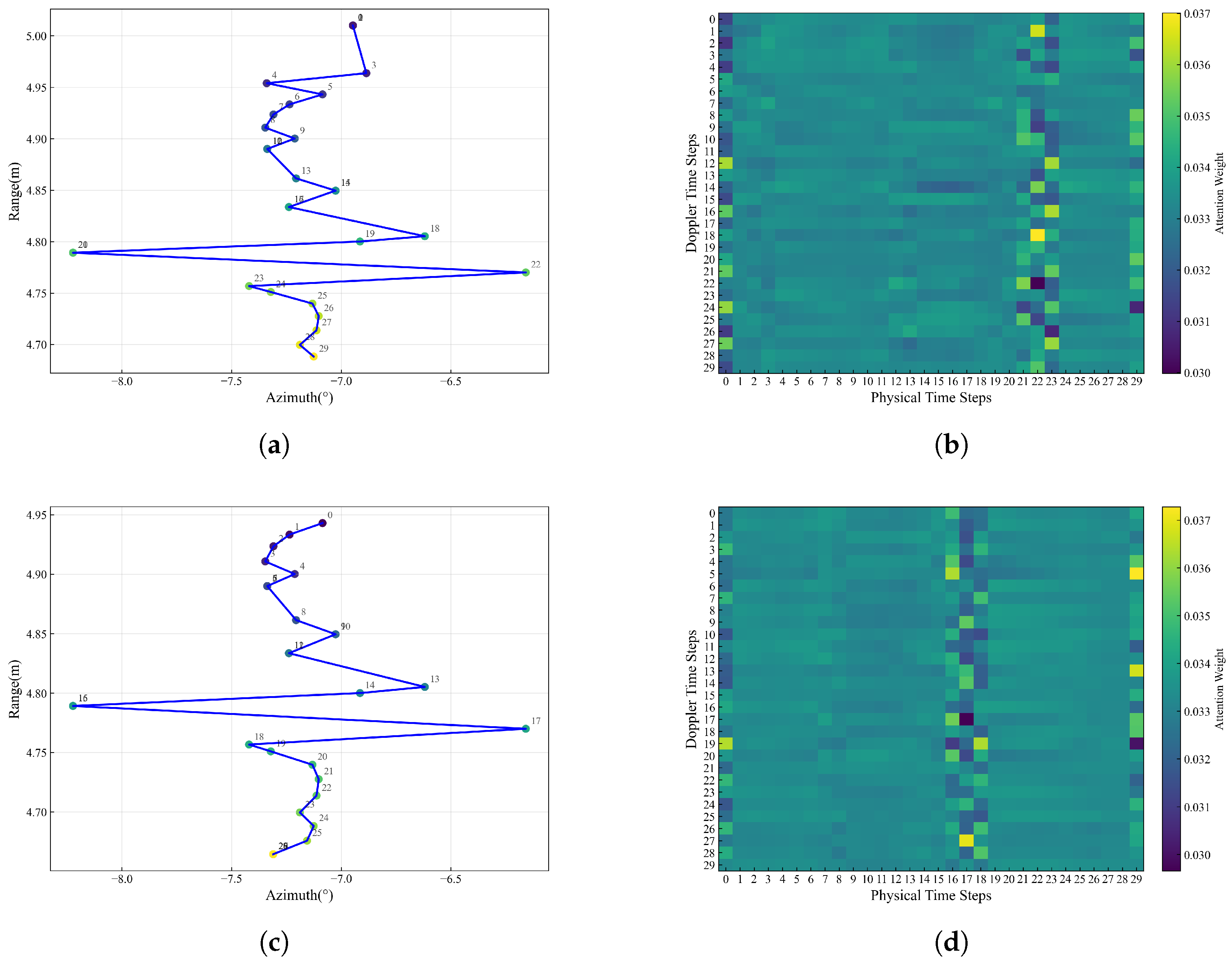
Figure 17 visualizes D → P attention weights alongside 2D trajectories of two rotor-drone samples.

In Sample 1, a motion change near time steps 21–23 coincides with higher attention responses. Sample 2 shows a similar pattern near steps 16–18. These observations indicate that the cross-attention module adaptively focuses on temporally correlated kinematic cues, not merely concatenating features. This aligns with the performance drop observed when cross-attention is ablated (Table 9).

6.5. Graph-Structure Hyperparameter Analysis

The effects of sequence length T and temporal neighborhood size $\tau$ are reported in

Table 10. Ablation results for graph-structure hyperparameters.

Setting	Fixed Parameter	Mean Acc (%)	Mean Lag (s)
Input sequence length T
$T=30$	$\tau =3$	99.73	24.58
$T=25$	$\tau =3$	98.80	20.48
$T=20$	$\tau =3$	97.74	16.38
$T=15$	$\tau =3$	96.59	12.29
$T=10$	$\tau =3$	87.32	8.19
$T=5$	$\tau =3$	59.37	4.10
Temporal neighbourhood size $\tau$
$\tau =1$	$T=30$	98.88	–
$\tau =2$	$T=30$	98.88	–
$\tau =3$	$T=30$	99.73	–
$\tau =4$	$T=30$	98.51	–
$\tau =5$	$T=30$	98.68	–
$\tau =6$	$T=30$	98.64	–

.

Accuracy degrades gradually as T decreases from 30 to 15, then sharply drops to 87.32% ($T=10$) and 59.37% ($T=5$), indicating that very short segments lack sufficient temporal context. The recognition lag (the time to form a track of T points, depending on the radar data rate) increases with T; $T=30$ offers the highest accuracy with an acceptable lag of 24.58 s.

For temporal neighborhood, $\tau =3$ achieves the best accuracy. Sparse connections ($\tau =1,2$) limit information flow, while larger $\tau$ values introduce redundant connections without further gain. Hence, $\tau =3$ is adopted.

6.6. Noise Robustness Analysis

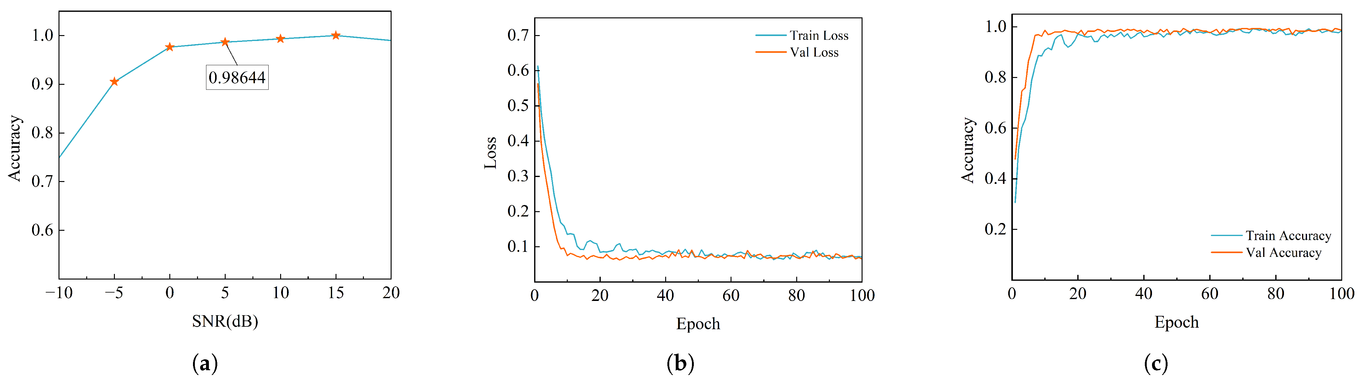
Figure 18 shows the model performance under different SNR conditions and the training dynamics at 5 dB. The model retains 74.92% accuracy at $-10$ dB, reaches 98.64% at 5 dB, and achieves 100% from 15 dB onward. The loss and accuracy curves under 5 dB converge stably, confirming robust learning.

Class-wise performance at 5 dB is detailed in

Table 11. Classification performance for each target type under SNR = 5 dB noise.

Target Type	Precision	Recall	F1-Score	Support
Passenger ship	1.0000	0.9592	0.9792	49
Speedboat	0.9583	1.0000	0.9787	46
Helicopter	1.0000	0.9535	0.9762	43
Rotor drone	1.0000	1.0000	1.0000	50
Bird	0.9796	1.0000	0.9897	48
Fixed-wing drone	0.9833	1.0000	0.9916	59
Macro Avg	0.9869	0.9854	0.9859	295
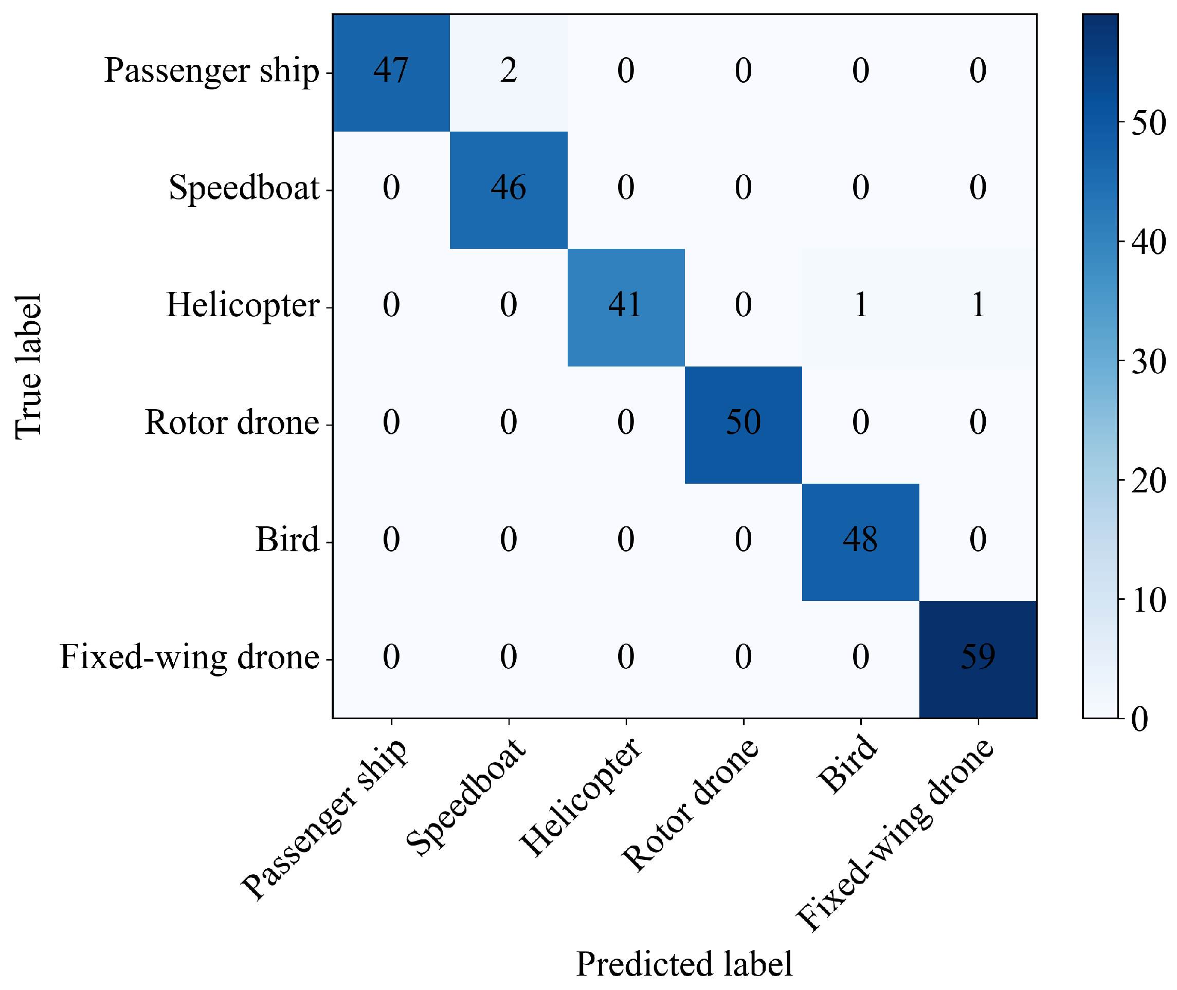
Weighted Avg	0.9868	0.9864	0.9864	295

. The macro F1-score is 0.9859. Rotor drone, bird, and fixed-wing drone achieve perfect recall. Only four misclassifications occur (Figure 19): two passenger ships confused with speedboats, and two helicopters misclassified as bird and fixed-wing drone. This limited confusion arises mainly between classes with partially overlapping motion characteristics under noise.

6.7. Validation on the LSS-PR-1.0 Dataset

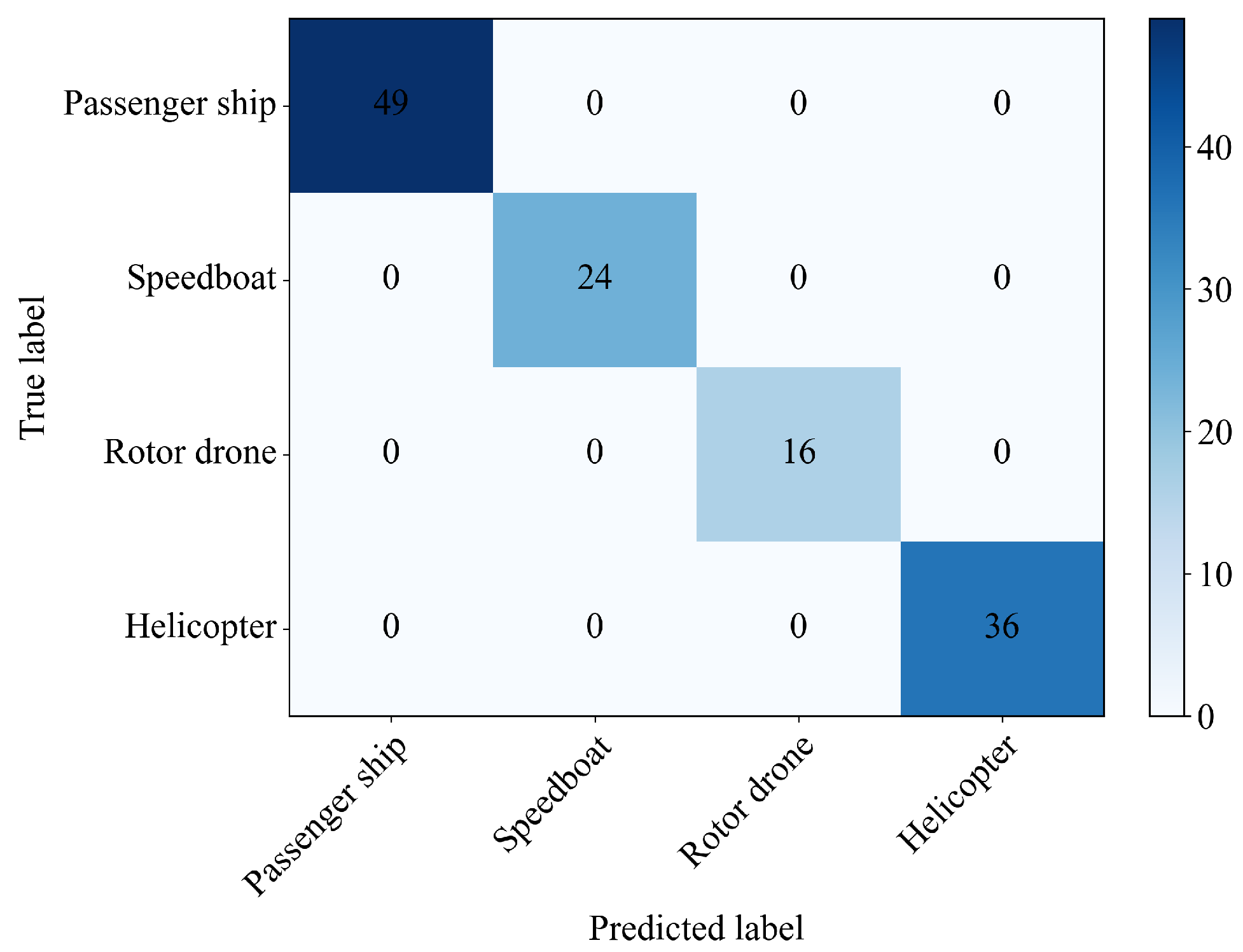
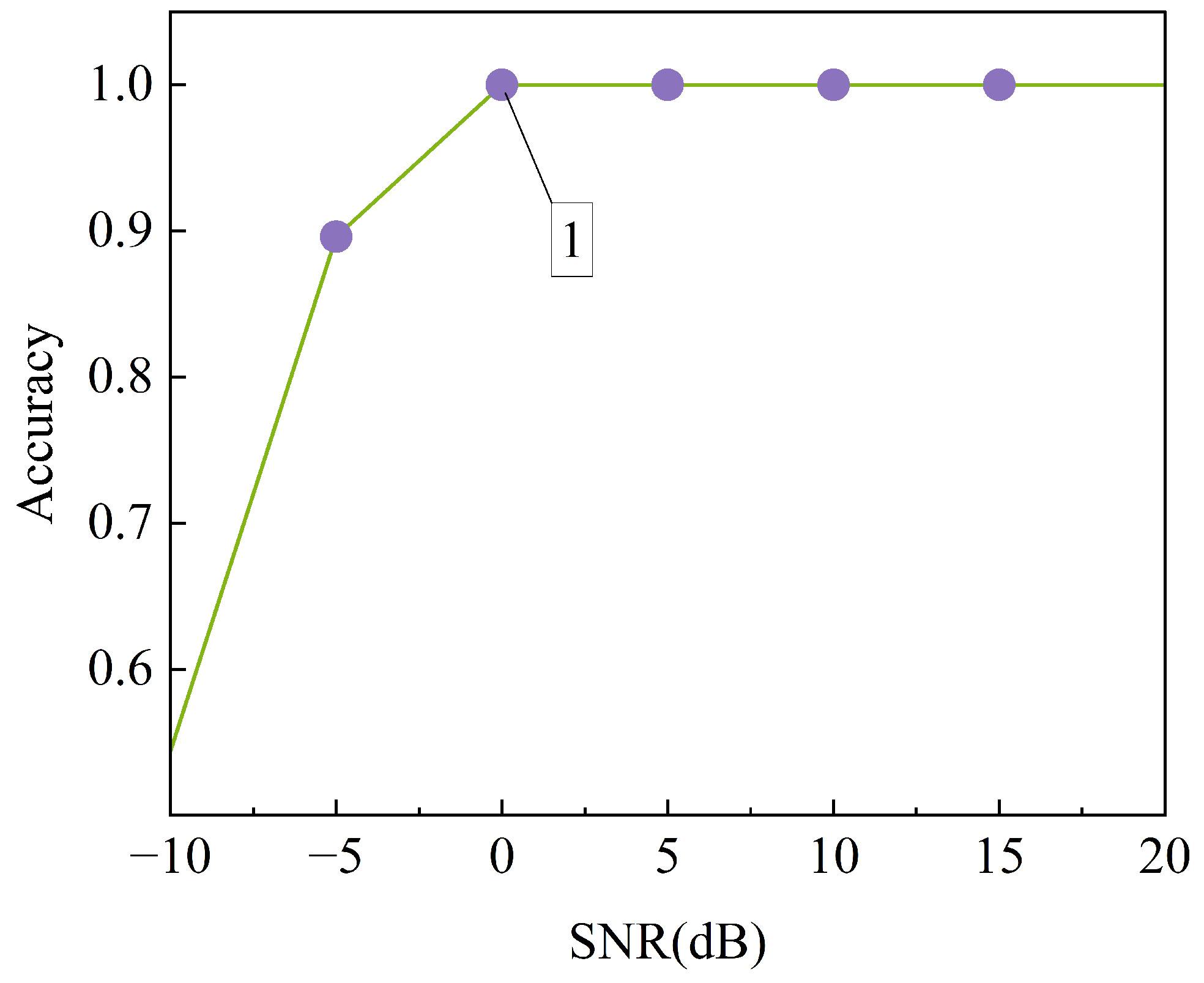
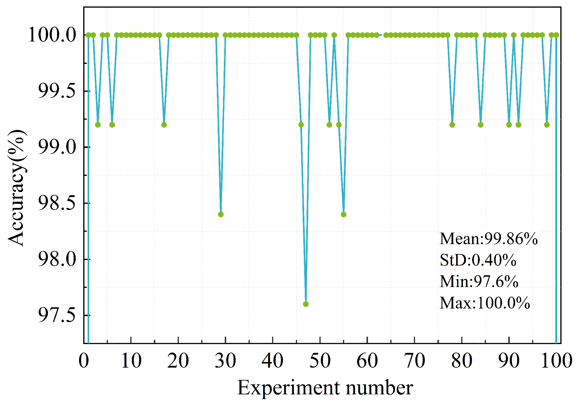
On LSS-PR-1.0, DS-STCAGCN achieves 100% accuracy at SNR ≥ 0 dB (Figure 20 and Figure 21). Over 100 independent runs, the average validation accuracy is 99.86% with 0.40% standard deviation; 86 runs reach 100%, and the minimum is 97.6% (Figure 22). These results confirm the framework’s strong generalization and stable convergence under a passive-radar modality.

7. Conclusions

This paper proposed DS-STCAGCN, a dual-stream spatio-temporal graph learning framework that combines Doppler-spectrum and kinematic features via separate encoding, bidirectional cross-attention, temporal self-attention, and graph convolution for LSS target recognition.

On LSS-DAUR-1.0, DS-STCAGCN achieves 99.73% mean accuracy over 10 runs, with only 0.22 M parameters and 3.21 ms inference latency, surpassing image-based, sequence-based, and handcrafted-feature baselines. t-SNE visualizations and ablation studies confirm the contributions of each module, while attention maps show that cross-attention adaptively associates Doppler-spectrum and kinematic cues. Under 5 dB SNR, the model retains 98.64% accuracy (macro F1 0.9859). On the passive-radar LSS-PR-1.0 dataset, it yields 99.86% average accuracy over 100 independent runs, demonstrating robust generalization across radar modalities.The proposed framework is general in methodology. In principle, it can be directly extended and applied without modifying the network architecture as long as new target categories possess similar multi-dimensional observation features (i.e., including Doppler-spectrum and kinematic parameters). This adaptability is preliminarily supported by its consistent performance across two distinct datasets with different class compositions.

Limitations include the need for validation under more complex scenarios (e.g., adverse weather, dense clutter) and the absence of fine-grained time-frequency modelling and adaptive graph-structure learning. Future work will address these aspects and explore lightweight deployment on embedded platforms.

Overall, DS-STCAGCN offers an effective spatio-temporal modelling approach for multi-dimensional radar sensing, indicating that Doppler–kinematic fusion with cross-modal attention and graph-based temporal modelling significantly improves LSS target representation.

References

- Patole, S.M.; Torlak, M.; Wang, D.; Ali, M. Automotive Radars: A review of signal processing techniques. IEEE Signal Process. Mag. 2017, 34, 22–35. [Google Scholar] [CrossRef]
- Chen, X.; Huang, Y.; Guan, J.; Song, W.; Xue, Y. Review of long-time integration technology for weak targets in MIMO radar. Signal Process. 2020, 36, 1947–1964. [Google Scholar] [CrossRef]
- He, Z.; Duan, J.; Lu, D. A review of radar sea target recognition technology. Sci. Technol. Rev. 2017, 35, 61–68. [Google Scholar] [CrossRef]
- Kumawat, H.C.; Chakraborty, M.; Raj, A.A.B.; Dhavale, S.V. DIAT-µSAT: Small aerial targets micro-Doppler signatures and their classification using CNN. IEEE Geosci. Remote Sens. Lett. 2021, 19, 6004005. [Google Scholar] [CrossRef]
- Park, D.; Lee, S.; Park, S.; Kwak, N. Radar-spectrogram-based UAV classification using convolutional neural networks. Sensors 2021, 21, 210. [Google Scholar] [CrossRef] [PubMed]
- Su, N.; Chen, X.; Guan, J.; Mou, X.; Liu, N. Detection and Classification of Maritime Target with Micro-motion Based on CNNs. J. Radars 2018, 7, 565–574. [Google Scholar] [CrossRef]
- Kim, Y.; Toomajian, B. Hand Gesture Recognition Using Micro-Doppler Signatures with Convolutional Neural Network. IEEE Access 2016, 4, 7125–7130. [Google Scholar] [CrossRef]
- Zhang, Y.; Zhang, S.; Liu, Y.; Jing, F. Radar HRRP Sequence Target Recognition Method of Attention Mechanism Based Stacked LSTM Network. Syst. Eng. Electron. 2021, 43, 2775–2781. [Google Scholar] [CrossRef]
- Yu, X.; Wei, S.; Fang, Y.; Sheng, J.; Zhang, L. Low-Altitude Slow Small Target Threat Assessment Algorithm by Exploiting Sequential Multifeature with Long Short-Term Memory. IEEE Sens. J. 2023, 23, 15524–15534. [Google Scholar] [CrossRef]
- Wang, J.; Chen, X.; Guan, J.; Su, N.; Yuan, W. A time-frequency representation method based on ETF-MDNet for radar target micro-motion features. Chin. J. Electron. 2025, 34, 1199–1208. [Google Scholar] [CrossRef]
- Song, Q.; Huang, S.; Zhang, Y.; Chen, X.; Chen, Z.; Zhou, X.; Deng, Z. Radar Target Classification Using Enhanced Doppler Spectrograms with ResNet34_CA in Ubiquitous Radar. Remote Sens. 2024, 16, 2860. [Google Scholar] [CrossRef]
- Wu, Q.; Chen, J.; Lu, Y.; Zhang, Y. A Complete Automatic Target Recognition System of Low Altitude, Small RCS and Slow Speed (LSS) Targets Based on Multi-Dimensional Feature Fusion. Sensors 2019, 19, 5048. [Google Scholar] [CrossRef] [PubMed]
- Yuan, W.; Chen, X.; Du, X.; Guan, J.; Wang, J.; Lan, T. A low slow small target classification network model based on K-band radar dynamic multifeature data fusion. IEEE Sens. J. 2025, 25, 1656–1668. [Google Scholar] [CrossRef]
- Chen, X.; Yuan, W.; Du, X.; Yu, G.; He, X.; Guan, J.; Wang, X. Multiband FMCW radar LSS-target detection dataset (LSS-FMCWR-1.0) and high-resolution micromotion feature extraction method. J. Radars 2024, 13, 539–553. [Google Scholar] [CrossRef]
- Zhao, Z.; Xu, S.; Shui, P. A Network Model for Sea Surface Small Targets Classification Based on Multidomain Radar Echo Data Fusion. J. Electron. Inf. Technol. 2025, 47, 696–706. [Google Scholar] [CrossRef]
- He, X.; Chen, X.; Du, X.; Su, N.; Yuan, W.; Guan, J. Maritime micro-motion target classification method based on CBAM-Swin-Transformer transfer learning. Syst. Eng. Electron. 2025, 47, 1155–1167. [Google Scholar] [CrossRef]
- Scarselli, F.; Gori, M.; Tsoi, A.C.; Hagenbuchner, M.; Monfardini, G. The graph neural network model. IEEE Trans. Neural Netw. 2009, 20, 61–80. [Google Scholar] [CrossRef] [PubMed]
- Khemani, B.; Patil, S.; Kotecha, K. A review of graph neural networks: Concepts, architectures, techniques, challenges, datasets, applications, and future directions. J. Big Data 2024, 11, 18. [Google Scholar] [CrossRef]
- Su, N.; Chen, X.; Guan, J.; Huang, Y. Maritime target detection based on radar graph data and graph convolutional network. IEEE Geosci. Remote Sens. Lett. 2021, 19, 4019705. [Google Scholar] [CrossRef]
- Su, N.; Chen, X.; Guan, J.; Huang, Y.; Wang, X.; Xue, Y. Radar maritime target detection via spatial–temporal feature attention graph convolutional network. IEEE Trans. Geosci. Remote Sens. 2024, 62, 5102615. [Google Scholar] [CrossRef]
- Lee, G.W.; Kim, J. MTGEA: A multimodal two-stream GNN framework for efficient point cloud and skeleton data alignment. Sensors 2023, 23, 2787. [Google Scholar] [CrossRef] [PubMed]
- Meng, H.; Peng, Y.X.; Wang, W.B.; Cheng, P.; Li, Y.; Xiang, W. Spatio-temporal-frequency graph attention convolutional network for aircraft recognition based on heterogeneous radar network. IEEE Trans. Aerosp. Electron. Syst. 2022, 58, 5548–5559. [Google Scholar] [CrossRef]
- Meng, H.; Peng, Y.; Wang, W. Dynamic graph network augmented by contrastive learning for radar target classification. In Proceedings of the 2024 IEEE Radar Conference, Denver, CO, USA, 6–10 May 2024; pp. 1–6. [Google Scholar] [CrossRef]
- Vaswani, A.; Shazeer, N.; Parmar, N.; Uszkoreit, J.; Jones, L.; Gomez, A.N.; Kaiser, Ł.; Polosukhin, I. Attention Is All You Need. arXiv 2017, arXiv:1706.03762. [Google Scholar] [CrossRef]
- Wu, Z.; Chen, J.; Al-Sabri, R.; Oloulade, B.M.; Gao, J. Depth-adaptive graph neural architecture search for graph classification. Knowl. Based Syst. 2024, 301, 112321. [Google Scholar] [CrossRef]
- Do, M.T.; Park, N.; Shin, K. Two-Stage Training of Graph Neural Networks for Graph Classification. Neural Process. Lett. 2023, 55, 2799–2823. [Google Scholar] [CrossRef]
- Xu, J.; Ni, J.; Ke, Y. A class-aware representation refinement framework for graph classification. Inf. Sci. 2024, 679, 121061. [Google Scholar] [CrossRef]
- Xie, Y.; Liang, Y.; Gong, M.; Qin, A.K.; Ong, Y.S.; He, T. Semisupervised Graph Neural Networks for Graph Classification. IEEE Trans. Cybern. 2023, 53, 6222–6235. [Google Scholar] [CrossRef] [PubMed]
- Chen, X.; Rao, G.; Guan, J.; Wang, J.; Wang, H.; Zhang, C.; Yi, J.; Wan, X.; Rao, Y. Passive radar low slow small detection dataset (LSS-PR-1.0) and multi-domain feature extraction and analysis methods. J. Radars 2025, 14, 249–268. [Google Scholar] [CrossRef]
- Baltrušaitis, T.; Ahuja, C.; Morency, L.-P. Multimodal Machine Learning: A Survey and Taxonomy. IEEE Trans. Pattern Anal. Mach. Intell. 2019, 41, 423–443. [Google Scholar] [CrossRef] [PubMed]
- Yan, S.; Xiong, Y.; Lin, D. Spatial Temporal Graph Convolutional Networks for Skeleton-Based Action Recognition. In Proceedings of the AAAI Conference on Artificial Intelligence, New Orleans, LA, USA, 2–7 February 2018; pp. 7444–7452. [Google Scholar]
- Richards, M.A. Fundamentals of Radar Signal Processing, 2nd ed.; McGraw-Hill Education: New York, NY, USA, 2014. [Google Scholar]
- LeCun, Y.; Bengio, Y.; Hinton, G. Deep learning. Nature 2015, 521, 436–444. [Google Scholar] [CrossRef] [PubMed]
- Han, J.; Pei, J.; Tong, H. Data Mining: Concepts and Techniques, 4th ed.; Morgan Kaufmann: Burlington, MA, USA, 2022. [Google Scholar]
- Bai, S.; Kolter, J.Z.; Koltun, V. An Empirical Evaluation of Generic Convolutional and Recurrent Networks for Sequence Modeling. arXiv 2018, arXiv:1803.01271. [Google Scholar]
- Nair, V.; Hinton, G.E. Rectified Linear Units Improve Restricted Boltzmann Machines. In Proceedings of the 27th International Conference on Machine Learning (ICML), Haifa, Israel, 21–24 June 2010; pp. 807–814. [Google Scholar]
- Lu, J.; Yang, J.; Batra, D.; Parikh, D. Hierarchical Question-Image Co-Attention for Visual Question Answering. In Advances in Neural Information Processing Systems; Curran Associates Inc.: Red Hook, NY, USA, 2016; pp. 289–297. [Google Scholar]
- Defferrard, M.; Bresson, X.; Vandergheynst, P. Convolutional Neural Networks on Graphs with Fast Localized Spectral Filtering. In Advances in Neural Information Processing Systems; Curran Associates Inc.: Red Hook, NY, USA, 2016; pp. 3844–3852. [Google Scholar]
- Kipf, T.N.; Welling, M. Semi-Supervised Classification with Graph Convolutional Networks. In Proceedings of the 5th International Conference on Learning Representations (ICLR), Toulon, France, 24–26 April 2017. [Google Scholar]
- Lin, M.; Chen, Q.; Yan, S. Network In Network. In Proceedings of the 2nd International Conference on Learning Representations (ICLR), Banff, AB, Canada, 14–16 April 2014. [Google Scholar]
- Goodfellow, I.; Bengio, Y.; Courville, A. Deep Learning; MIT Press: Cambridge, MA, USA, 2016. [Google Scholar]
- Bagnall, A.; Lines, J.; Bostrom, A.; Large, J.; Keogh, E. The Great Time Series Classification Bake off: A Review and Experimental Evaluation of Recent Algorithmic Advances. Data Min. Knowl. Discov. 2017, 31, 606–660. [Google Scholar] [CrossRef] [PubMed]
- Sutskever, I.; Vinyals, O.; Le, Q.V. Sequence to Sequence Learning with Neural Networks. In Advances in Neural Information Processing Systems; Curran Associates Inc.: Red Hook, NY, USA, 2014; pp. 3104–3112. [Google Scholar]
- Fey, M.; Lenssen, J.E. Fast Graph Representation Learning with PyTorch Geometric. arXiv 2019, arXiv:1903.02428. [Google Scholar]
- Loshchilov, I.; Hutter, F. Decoupled Weight Decay Regularization. In Proceedings of the 7th International Conference on Learning Representations (ICLR), New Orleans, LA, USA, 6–9 May 2019. [Google Scholar]
- Srivastava, N.; Hinton, G.; Krizhevsky, A.; Sutskever, I.; Salakhutdinov, R. Dropout: A Simple Way to Prevent Neural Networks from Overfitting. J. Mach. Learn. Res. 2014, 15, 1929–1958. [Google Scholar]
- Ioffe, S.; Szegedy, C. Batch Normalization: Accelerating Deep Network Training by Reducing Internal Covariate Shift. In Proceedings of the 32nd International Conference on Machine Learning (ICML), Lille, France, 6–11 July 2015; pp. 448–456. [Google Scholar]
- Pedregosa, F.; Varoquaux, G.; Gramfort, A.; Michel, V.; Thirion, B.; Grisel, O.; Blondel, M.; Prettenhofer, P.; Weiss, R.; Dubourg, V.; et al. Scikit-learn: Machine Learning in Python. J. Mach. Learn. Res. 2011, 12, 2825–2830. [Google Scholar]
- Chen, T.; Guestrin, C. XGBoost: A Scalable Tree Boosting System. In Proceedings of the 22nd ACM SIGKDD International Conference on Knowledge Discovery and Data Mining, San Francisco, CA, USA, 13–17 August 2016; pp. 785–794. [Google Scholar] [CrossRef]
Figure 1.
The data cube of range-Doppler-frame. Orange region: range cell containing the target; purple region: micro-Doppler spectrum obtained from one CPI.
Figure 2.
Frame-level node attributes composed of Doppler-spectrum and kinematic features.
Figure 3.
The edge construction process.
Figure 4.
Architecture of DS-STCAGCN.
Figure 5.
Schematic diagram of Doppler-to-kinematic cross-attention.
Figure 6.
Schematic diagram of the temporal attention mechanism.
Figure 7.
Schematic diagram of graph convolution layers.
Figure 8.
Schematic diagram of the classification decision layer.
Figure 9.
Various target images. (a) passenger ship. (b) speedboat. (c) helicopter. (d) rotor drone. (e) bird. (f) fixed-wing drone.
Figure 10.
Boxplots of kinematic distributions for each target class based on the full dataset. (a) Velocity boxplots. (b) Acceleration boxplots.
Figure 11.
DWD for each type of target. (a) passenger ship. (b) speedboat. (c) helicopter. (d) rotor drone. (e) bird. (f) fixed-wing drone.
Figure 12.
Three-dimensional tracks for each type of target. (a) passenger ship. (b) speedboat. (c) helicopter. (d) rotor drone. (e) bird. (f) fixed-wing drone.
Figure 13.
Representative DWD for the LSS-PR-1.0 dataset. (a) passenger ship. (b) speedboat. (c) rotor drone. (d) helicopter.
Figure 14.
Representative 2D trajectories for the LSS-PR-1.0 dataset. (a) passenger ship. (b) speedboat. (c) rotor drone. (d) helicopter.
Figure 15.
Best validation accuracy curves of different models.
Figure 16.
t-SNE visualization of feature distributions at different representation stages.
Figure 17.
Visualization of 2D trajectories and D→P attention weights for two rotor UAV samples: (a) Sample 1’s 2D trajectory; (b) Sample 1’s D→P attention weights heatmap; (c) Sample 2’s 2D trajectory; (d) Sample 2’s D→P attention weights heatmap.
Figure 18.
Noise robustness analysis of DS-STCAGCN. (a) Accuracy under different SNR conditions (star markers denote the results at each tested SNR level). (b) Training and validation loss curves under SNR = 5 dB. (c) Training and validation accuracy curves under SNR = 5 dB.
Figure 19.
Confusion matrix of DS-STCAGCN under SNR = 5 dB noise.
Figure 20.
Confusion matrix of DS-STCAGCN on the LSS-PR-1.0 dataset under SNR = 5 dB noise.
Figure 21.
Accuracy of DS-STCAGCN on the LSS-PR-1.0 dataset under different SNR conditions.
Figure 22.
Distribution of validation accuracy over 100 independent training runs on the LSS-PR-1.0 dataset.