Enhanced Mainlobe Jamming Suppression in Distributed Array Radar via Joint Optimization of Radar Positions and Subpulse Frequencies

Abstract

This study presents a joint optimization framework for radar positions and subpulse carrier frequencies to address mainlobe jamming suppression in a distributed array radar system with one main and multiple auxiliary radars. Accounting for gain and aperture differences between the main and auxiliary radars, the grating lobe effect on jamming suppression performance is analyzed. Unlike conventional sparse array design approaches, this work introduces an architecture leveraging subpulses at distinct carrier frequencies to enhance grating lobe suppression and jamming suppression. A specific joint optimization method for radar positions and subpulse frequencies is then established. With jamming suppression performance as the objective function, the method first maps the variations induced by a range of candidate frequencies onto a single representative frequency point. This mapping enables efficient optimization of radar positions across the designated frequency band. Subsequently, a sequential scheme selects specific carrier frequencies for the subpulses. In practical anti-jamming operations, the optimal frequency for the current scenario is determined by analyzing the suppression results from these subpulses. The main radar then transmits pulses at this optimal frequency, thereby reducing both system complexity and pulse accumulation difficulty. Simulation results demonstrate that the proposed method achieves a reduction of over 3 dB in grating lobe suppression compared to conventional sparse array design methods, while enhancing the output signal-to-jamming and noise ratio by nearly 3 dB after jamming suppression.

1. Introduction

The intensity of electronic warfare on modern battlefields continues to escalate, and the jamming threats faced by radar systems are becoming increasingly severe [1,2]. Spatially, radar jamming can be categorized into sidelobe jamming [3] and mainlobe jamming [4]. For sidelobe jamming, conventional phased array radars [5,6] can effectively suppress jamming using techniques such as adaptive beamforming [7] or sidelobe cancellers [8]. However, when the jammer and the target are both located within the mainlobe, forming mainlobe jamming, the jamming signal is amplified by the mainlobe gain, resulting in higher energy. Furthermore, due to limitations in angular resolution, the radar cannot suppress the jamming signal while simultaneously preserving the target signal. This severely compromises the target detection capabilities of radar [9,10].

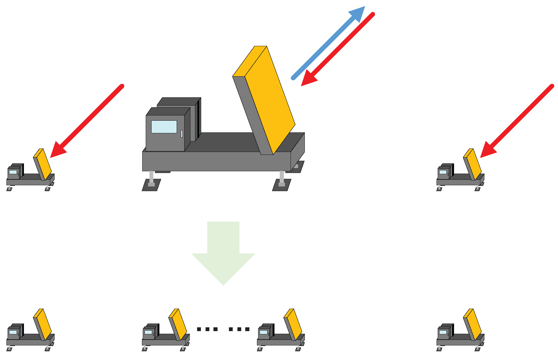
Distributed array radar systems deploy multiple radar nodes over a long baseline to achieve exceptionally high angular resolution [11,12,13]. When countering mainlobe jamming, these systems can form extremely narrow nulls to suppress jamming signals while preserving the energy of target signals [14]. In practical applications, a main-auxiliary distributed array radar configuration is often employed. This setup involves deploying one main radar capable of both transmitting and receiving signals, along with a small number of auxiliary radars that are only capable of receiving signals, over a long baseline [15]. Essentially, the distributed array radar leverages its long-baseline deployment to convert the mainlobe jamming of the main radar into sidelobe jamming for the entire array, thereby enabling effective suppression through spatial beamforming techniques. In such a design, the auxiliary radars are fewer in number and do not require signal transmission capability, which effectively reduces system costs and enhances the implementation feasibility. Authors of [16] developed a cost-effective receive-only auxiliary radar architecture utilizing a commercial chip that integrates all essential radio frequency, mixed-signal, and digital modules to achieve full receiver capabilities. Existing research on anti-jamming techniques for this kind of distributed array radar primarily focuses on algorithm design. For example, researchers of [17] proposed an algorithm that enhances anti-jamming performance by dividing signals into subbands. Additionally, authors of [18] introduced a joint suppression algorithm for jamming and clutter based on the generalized inner product in distributed array radar systems.

Due to the sparse deployment of distributed array radars over long baselines, the occurrence of grating lobes is unavoidable. Existing research primarily focuses on sparse array design to suppress grating lobes or sidelobes. For instance, the chaos sparrow search algorithm (CSSA) in [19] synthesized sparse planar arrays with low peak sidelobe levels and improved convergence efficiency, combining density-weighted methods with chaotic mapping for element position optimization. Similarly, a research group of [20] introduced a discrete slime mold algorithm (DSMA) for ultrasonic sensor arrays, which achieved sidelobe suppression by optimizing array sparsity while reducing computational complexity. The water cycle algorithm (WCA) was also applied to design low-sidelobe beam patterns with wide nulling capabilities [21]. Other works have explored hybrid optimization techniques such as quantum particle swarm optimization (QPSO) [22], enhanced Harris hawks optimization (EHHO) [23], and adaptive genetic algorithms (AGA) with self-supervised differential operators [24] to address grating lobe suppression. These algorithms primarily aim to reduce the impact of grating lobes by optimizing the positions of array nodes, often assuming the presence of dozens or even hundreds of nodes. However, in the case of a distributed array radar with one main and a few auxiliary nodes deployed over a long baseline, adjusting node positions alone is insufficient to effectively reduce the grating lobe levels.

For distributed array radar systems, the location of grating lobes is influenced not only by the positions of the nodes but also by the operating frequency. Authors of [25] proposed a dual-frequency method that performs unambiguous direction-of-arrival estimation through phase differencing between frequencies, mitigating grating lobe ambiguities during target observation. Although this algorithm cannot be applied to jamming suppression, introducing frequency to address grating lobes is indeed an approach worth referencing.

To fully account for the characteristics of main-auxiliary distributed array radar systems and achieve comprehensive grating lobe suppression, this paper proposes a novel joint optimization algorithm that simultaneously designs both radar positions and subpulse carrier frequencies, with particular emphasis on mainlobe jamming suppression performance. The algorithm optimizes radar positions and designs multiple subpulses with different frequencies, ensuring that the distributed array radar achieves the optimal output signal-to-jamming and noise ratio (SJNR) for jamming signals appearing at any angle within the mainlobe. In this paper, the formation of grating nulls in spatial domain adaptive processing for distributed array radar is analyzed based on beamforming principles. To address the gain and aperture inconsistencies between the main and auxiliary radars, a grating lobe optimization model is developed for a distributed array radar system with one main radar and multiple auxiliary radars. Building on this, a novel strategy for mainlobe jamming suppression is introduced, incorporating multiple subpulses with different frequencies. Frequency is introduced as an optimization parameter in grating lobe suppression by mapping a frequency range onto a specific angular range at a single frequency point, effectively integrating frequency into the radar position optimization process. Radar positions are first optimized using a constrained particle swarm optimization (PSO) algorithm, followed by further optimization of subpulse frequencies to minimize the highest peak grating lobe. In a specific scenario, the optimal frequency is unique, while other frequencies degrade system performance. Furthermore, frequent switching between different frequency pulses increases system complexity and complicates pulse accumulation. To address this, this paper proposes an optimal frequency selection strategy based on output SJNR. The system then transmits pulses at this frequency exclusively in this scenario, thereby improving performance while avoiding unnecessary frequency switching. Finally, simulations are conducted to validate the proposed model and algorithm. The results demonstrate the effectiveness of the proposed approach in enhancing anti-jamming performance. This study further verifies the effectiveness of the SJNR-based optimal frequency selection strategy through dynamic scenario simulation.

The organization of the paper is as follows: Section 1 introduces the research background and highlights the main contributions of this study. Section 2 details the signal model and optimization model. Section 3 outlines the proposed algorithm. Section 4 presents the simulation results to validate the algorithm. Finally, Section 5 concludes the paper.

2. System Overview

2.1. Signal Model

To address the issue of inconsistent antenna gain and aperture between the auxiliary radars and the main radar, the main radar is decomposed into multiple subarrays with the same gain as the auxiliary radars, uniformly distributed across the aperture of the main radar. This decomposition facilitates subsequent modeling. In this study, the distributed array radar is used exclusively for mainlobe jamming suppression. As such, even if the spacing between the decomposed subarrays exceeds half a wavelength, it does not affect the modeling of signals within the mainlobe angular range. A schematic diagram of the distributed array radar is shown in Figure 1.

Due to practical deployment constraints, ground-based distributed array radars are typically designed to improve angular resolution in azimuth for mainlobe jamming suppression. Therefore, only a one-dimensional array needs to be considered. Furthermore, the proposed design does not impose constraints on the antenna architecture of auxiliary radars. As demonstrated in [16], different types of antennas can also be combined to form a distributed array radar system. In practical implementations, parabolic antenna-based auxiliary radars could be adopted to further reduce system costs while maintaining the validity of the proposed method.

Without loss of generality, the full array echo for a scenario involving a mainlobe jamming of the main radar and a single target is expressed in (1). In this paper, all subsequent references to “mainlobe jamming” denote the mainlobe jamming of the main radar.

$$\mathbf{s}\left(t\right)=\mathbf{a}\left({\theta }_0\right){\mathbf{s}}_0\left(t\right)+\mathbf{a}\left({\theta }_j\right){\mathbf{s}}_j\left(t\right)+\mathbf{N}\left(t\right)$$

(1)

In the equation, $\mathbf{a}\left({\theta }_0\right)$ and $\mathbf{a}\left({\theta }_j\right)$ are K-dimensional column steering vectors of target and jamming, where K represents the total number of channels, comprising the subarrays of the main radar and the auxiliary radars. Specifically, the main radar consists of M subarrays, and there are $M^{\prime }$ auxiliary radars. Therefore, $K=M+M^{\prime }$. All channels are assumed to have identical gain, which remains constant within the mainlobe range of the main radar. ${\mathbf{s}}_0\left(t\right)$ and ${\mathbf{s}}_j\left(t\right)$ represent the complex envelopes of the target and the jamming, respectively, and $\mathbf{N}\left(t\right)$ denotes the noise matrix.

In theory, spatial domain jamming suppression does not impose specific constraints on the type of the jamming; it only focuses on the steering vector of the jamming signal. Since repeater deception jamming can be mitigated using mismatched filters [26] or other time-frequency domain processing methods [27,28], this paper primarily discusses barrage jamming, which exhibits more random time-frequency characteristics and is better suited for suppression in the spatial domain. The jammer continuously intercepts and analyzes the radar’s transmitted signal while simultaneously emitting barrage jamming at the same frequency as the radar signal.

To improve anti-jamming performance through grating lobe optimization, the primary step involves analyzing how grating lobes affect spatial jamming suppression capability. This requires establishing the exact mathematical relationship between the grating lobe and the output SJNR after jamming suppression.

The optimal weight vector for spatial jamming suppression [29] can be expressed in (2).

$$\mathbf{w}={\displaystyle \frac{{\mathbf{R}}^{-1}\mathbf{a}\left({\theta }_0\right)}{{\mathbf{a}}^H\left({\theta }_0\right){\mathbf{R}}^{-1}\mathbf{a}\left({\theta }_0\right)}}$$

(2)

$\mathbf{R}$ is the jamming-plus-noise covariance matrix. In practice, approximate jamming-plus-noise covariance matrices can be obtained through some sample selection methods [18].

The output SJNR achieved with this weight vector is given by (3).

$$\begin{array}{cc}\hfill \mathrm{SJN}{\mathrm{R}}_{out}& ={\displaystyle \frac{{\mathbf{w}}^H\mathbf{a}\left({\theta }_0\right)E\left[{\mathbf{s}}_0^2\left(t\right)\right]{\mathbf{a}}^H\left({\theta }_0\right)\mathbf{w}}{{\mathbf{w}}^H\mathbf{Rw}}}\hfill \\ \hfill & ={\displaystyle \frac{E\left[{\mathbf{s}}_0^2\left(t\right)\right]}{\frac{{\mathbf{a}}^H\left({\theta }_0\right){\mathbf{R}}^{-1}}{{\mathbf{a}}^H\left({\theta }_0\right){\mathbf{R}}^{-1}\mathbf{a}\left({\theta }_0\right)}\mathbf{R}\frac{{\mathbf{R}}^{-1}\mathbf{a}\left({\theta }_0\right)}{{\mathbf{a}}^H\left({\theta }_0\right){\mathbf{R}}^{-1}\mathbf{a}\left({\theta }_0\right)}}}\hfill \\ \hfill & =E\left[{\mathbf{s}}_0^2\left(t\right)\right]{\mathbf{a}}^H\left({\theta }_0\right){\mathbf{R}}^{-1}\mathbf{a}\left({\theta }_0\right)\hfill \end{array}$$

(3)

$E\left[•\right]$ denotes the expected value.

The jamming signal and noise are assumed to be independent and uncorrelated. Based on the signal model, $\mathbf{R}$ in (3) can be expressed as

$$\begin{array}{cc}\hfill \mathbf{R}& =E\left[{\mathbf{s}}_{j+N}\left(t\right){\mathbf{s}}_{j+N}^H\left(t\right)\right]\hfill \\ \hfill & ={\sigma }_j^2\mathbf{a}\left({\theta }_j\right){\mathbf{a}}^H\left({\theta }_j\right)+{\sigma }_n^2\mathbf{I}\hfill \end{array}$$

(4)

In which:

$${\mathbf{s}}_{j+N}\left(t\right)=\mathbf{a}\left({\theta }_j\right){\mathbf{s}}_j\left(t\right)+\mathbf{N}\left(t\right)$$

(5)

${\sigma }_j^2$ represents the jamming power, ${\sigma }_n^2$ denotes the noise power, and $\mathbf{I}$ is the identity matrix.

To compute the inverse matrix of $\mathbf{R}$, we apply the Sherman–Morrison formula [30] as follows:

$${(\mathbf{A}+\mathbf{u}{\mathbf{v}}^H)}^{-1}={\mathbf{A}}^{-1}-{\displaystyle \frac{{\mathbf{A}}^{-1}\mathbf{u}{\mathbf{v}}^H{\mathbf{A}}^{-1}}{1+{\mathbf{v}}^H{\mathbf{A}}^{-1}\mathbf{u}}}$$

(6)

Substituting (4) into (6) yields the ${\mathbf{R}}^{-1}$, as derived in (7).

$${\mathbf{R}}^{-1}={\sigma }_n^{-2}\left[\mathbf{I}-{\displaystyle \frac{{\epsilon }_j\mathbf{a}\left({\theta }_j\right){\mathbf{a}}^H\left({\theta }_j\right)}{1+{\epsilon }_{j}K}}\right]$$

(7)

${\epsilon }_j$ represents the ratio of total jamming power to total noise power for a single channel.

Substituting (7) into (3), we obtain:

$$\begin{array}{cc}\hfill {\mathrm{SJNR}}_{out}& =E\left[{\mathbf{s}}_0^2\left(t\right)\right]{\mathbf{a}}^H\left({\theta }_0\right){\mathbf{R}}^{-1}\mathbf{a}\left({\theta }_0\right)\hfill \\ \hfill & ={\epsilon }_s\left[K-{\displaystyle \frac{{\epsilon }_j{\left|{\mathbf{a}}^H\left({\theta }_0\right)\mathbf{a}\left({\theta }_j\right)\right|}^2}{1+{\epsilon }_{j}K}}\right]\hfill \end{array}$$

(8)

${\epsilon }_s$ represents the original SNR of the target signal.

When the jamming-to-noise power ratio ${\epsilon }_j$ is sufficiently large, Equation (8) can be simplified as

$${\mathrm{SJNR}}_{out}\approx {\epsilon }_s\left[K-{\displaystyle \frac{{\left|{\mathbf{a}}^H\left({\theta }_0\right)\mathbf{a}\left({\theta }_j\right)\right|}^2}{K}}\right]$$

(9)

From (9), it can be observed that the output SJNR is determined by the inner product between the target steering vector and the jamming steering vector, which represents the spatial correlation between the target and the jamming.

In a distributed array radar system with a small number of radars deployed over a long baseline, grating lobes inevitably arise. When the jamming is located at the grating lobe position corresponding to the target angle, the target steering vector and the jamming steering vector become highly correlated. According to (9), this results in a loss of output SJNR, as the adaptive beamforming pattern forms a grating null at the target location.

It is evident that when the target angle is fixed and the jamming appears at any angle within the mainlobe, the output SJNR after jamming suppression is positively correlated with the gain of the conventional beam pattern at the jamming location. Therefore, to achieve higher output SJNR, it is essential to minimize the peak grating lobe level (PGLL) of the conventional beam pattern for the entire array.

2.2. Optimization Model

${\left|{\mathbf{a}}^H\left({\theta }_0\right)\mathbf{a}\left({\theta }_j\right)\right|}^2$ can be derived as:

$${\left|\rho \right|}^2={\left|{\mathbf{a}}^H\left({\theta }_0\right)\mathbf{a}\left({\theta }_j\right)\right|}^2={\left|\sum _{i=1}^K{e}^{j2\pi f{d}_i\left(sin{\theta }_j-sin{\theta }_0\right)}\right|}^2$$

(10)

In (10), the value of the inner product between the steering vectors depends not only on the angles of the target and jamming and the radar positions $d_i$, but also on the carrier frequency f. By selecting appropriate carrier frequencies, it is possible to avoid jamming appearing at the grating lobe position of the target. Optimizing radar positions $d_i$ and signal carrier frequency f can enhance the output SJNR when the jamming is located at angle ${\theta }_j$ and the target is located at angle ${\theta }_0$. This leads to the following optimization problem:

$$\underset{d_1,\cdots ,d_K,f}{min}{\left|\rho \left(d,f\right)\right|}^2$$

(11)

However, in practice, the angles of the jamming and the target can vary. To address this, this paper proposes a multi-frequency subpulse jamming suppression scheme. In this approach, the main radar transmits a series of subpulses with different carrier frequencies. The pulses differ only in pre-designed carrier frequencies. Each pulse echo undergoes independent spatial adaptive filtering and output. The core concept is that through joint optimization of radar positions and carrier frequencies, regardless of the jamming angle within the mainlobe, at least one carrier frequency will achieve minimized PGLL, thereby obtaining ideal output SJNR in the jamming suppression result. A schematic of this approach is shown in Figure 2.

As indicated by (10), if the radar uses multiple carrier frequencies for jamming suppression, it is equivalent to varying the carrier frequency term f to scale the angular term $sin{\theta }_j-sin{\theta }_0$. Therefore, the effect of carrier frequency variation on the beam pattern can be equivalently interpreted as scaling along the angular dimension, as illustrated in Figure 3.

The Figure 3 shows the beam pattern responses of a distributed array radar at three different carrier frequencies when the beam is pointing at 0°. It can be observed that switching between different carrier frequencies is equivalent to scaling along the angular dimension. Since the variation of $sin{\theta }_j-sin{\theta }_0$ and ${\theta }_j-{\theta }_0$ is not linear, the amount of scaling increases as ${\theta }_j$ becomes larger.

Assuming the beam points to 0°, the angular expansion range corresponding to the frequency range can be calculated using (10). Let the center frequency be $f_0$ and the frequency variation range be $\Delta f$. This relationship is shown in (12).

$$\begin{array}{cc}\hfill {\left|{\rho }_{f_0+\Delta f}\right|}^2& ={\left|\sum _{i=1}^K{e}^{j2\pi d_i\left(f_0+\Delta f\right)\left(sin{\theta }_j\right)}\right|}^2\hfill \\ \hfill & ={\left|\sum _{i=1}^K{e}^{j2\pi d_i{f}_0\left(1+{\displaystyle \frac{\Delta f}{f_0}}\right)\left(sin{\theta }_j\right)}\right|}^2\hfill \end{array}$$

(12)

As seen from (12), when switching carrier frequencies, the response at frequency $f_0+\Delta f$ at $sin{\theta }_j$ is equivalent to the response at frequency $f_0$ at $\left(1+{\displaystyle \frac{\Delta f}{f_0}}\right)sin{\theta }_j$. Consequently, under the multi-frequency scheme, the jamming suppression performance at a given angle depends on the minimum beampattern response within the angular range scaled by the multiple frequencies. Therefore, when the frequency variation range is $\left[f_0-\Delta f,f_0+\Delta f\right]$, the optimization problem is defined as

$$\begin{array}{c}\underset{d_1,\cdots ,d_i,\cdots ,d_{M^{\prime }+1}}{min}\mathrm{PGLL}\hfill \\ \left\{\begin{array}{c}\mathrm{PGLL}=maxL\left({\theta }_j\right){\theta }_j\in \Phi \hfill \\ L\left({\theta }_j\right)=min{\left|\rho \left(d_i,{{\theta }^{\prime }}_j\right)\right|}^2{{\theta }^{\prime }}_j\in \left[arcsin\left({\displaystyle \frac{f_0+\Delta f}{f_0}}sin{\theta }_j\right),arcsin\left({\displaystyle \frac{f_0-\Delta f}{f_0}}sin{\theta }_j\right)\right]\hfill \\ \left|d_{i^{\prime }}-d_i\right|\ge d_{c}i\ne i^{\prime }\hfill \\ max\left(d_i\right)-min\left(d_i\right)=l\hfill \end{array}\right.\hfill \end{array}$$

(13)

$\Phi$ represents the angular range to be optimized, which lies within the mainlobe of the main radar but outside the mainlobe of the entire array. Since the positions of the multiple subarrays of the main radar are determined by the central position of the main radar, the actual number of radar positions to be optimized $M^{\prime }+1$. In practice, due to constraints such as radar size and electromagnetic compatibility requirements, the minimum spacing between radars must be greater than $d_c$. The total baseline length is l.

The frequency variation range of a radar system typically varies due to hardware differences. In this study, we refer to the frequency-agile radar configurations discussed in [31,32] to design the frequency variation range. Additionally, the minimum frequency step is dictated by the radar’s bandwidth to avoid interference between signals operating at different frequencies.

Moreover, according to (10), assuming the azimuth angle of the target increases while the angular separation between the target and the jamming remains constant, the value of $sin{\theta }_j-sin{\theta }_0$ decreases as ${\theta }_0$ increases. This reflects an expansion in the beam pattern response. The PGLL of the expanded beam pattern will not exceed the optimized PGLL when the target is at 0°. Therefore, optimization is only required for the case where the target is at 0°. This theory will be further validated through simulations in this paper.

3. Joint Optimization of Positions and Carrier Frequencies

Clearly, the optimization problem in (13) is non-convex. This paper employs the PSO algorithm [33] to solve the problem in (13). The PSO algorithm, as a multi-objective optimization method, treats the main radar position as a distinct element within a particle for optimization. Additionally, the PSO algorithm’s search mechanism—guided by both the global best solution and personal best solutions—effectively ensures that particles remain within the baseline length constraints. A stepwise optimization strategy is then employed to select the subpulse frequencies.

3.1. Radar Position Optimization Based on the PSO Algorithm

3.1.1. Constrained Initialization

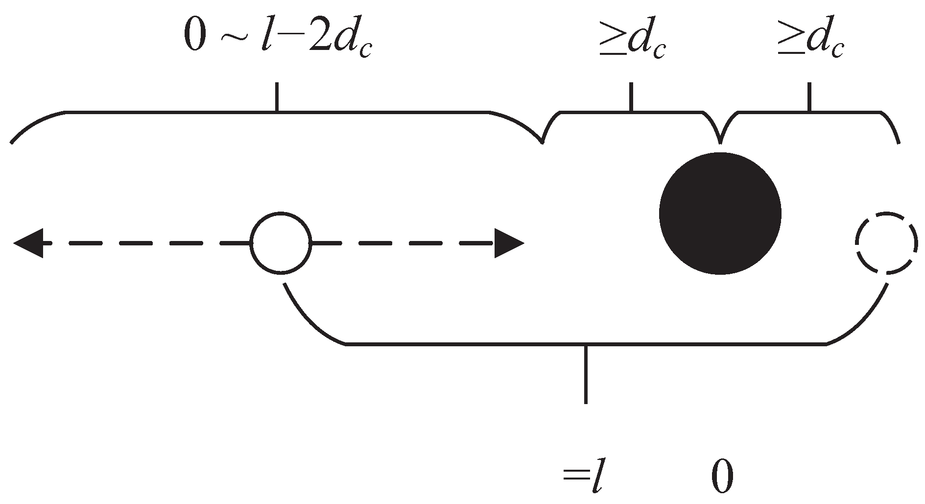
Considering the differences between the main and auxiliary radars, the position of the main radar must be treated as a separate parameter for optimization. Therefore, during particle initialization, this paper generates positions based on the main radar as a reference, as shown in Figure 4. The black dot represents the main radar, while the white dots represent the auxiliary radars.

With constraints on the baseline length l and the minimum spacing $d_c$, the main radar is positioned at 0. The leftmost radar is generated first and is randomly positioned within a range of length $l-2d_c$. Once the leftmost radar is generated, the position of the rightmost radar can be determined based on the baseline length constraint. The existing three nodes occupy a total space of $4d_c$. To strictly ensure that the spacing between radars exceeds $d_c$, the remaining $M^{\prime }-2$ auxiliary radars still require $\left(M^{\prime }-3\right)d_c$ spacing. Therefore, the remaining radars are generated within the range of length $l-\left(M^{\prime }+1\right)d_c$, followed by adjustments made according to the positions of existing radars.

After all radar positions are generated, a collective translation is applied to the entire set such that the leftmost radar is positioned at 0 and the rightmost radar is positioned at l. In this paper, such a set of radar positions is considered as a particle $\mathbf{d}$. Particles are generated sequentially to form the particle swarm $\mathbf{D}$.

3.1.2. Fitness Calculation

Due to the symmetry of the antenna beam pattern, it is only necessary to calculate the fitness within half of the angular range. Additionally, as this paper focuses on mainlobe jamming, only the angular range within the mainlobe of the main radar needs to be considered. Thus, the optimization is confined to angles outside the mainlobe of the entire array but within the mainlobe of the main radar.

Using the multi-frequency mapping method described in Section 2.2, the angular range corresponding to the frequency range can be calculated. Under specific parameter settings, the angular expansion range $\left[arcsin\left({\displaystyle \frac{f_0+\Delta f}{f_0}}sin{\theta }_j\right),arcsin\left({\displaystyle \frac{f_0-\Delta f}{f_0}}sin{\theta }_j\right)\right]$ for each angle at the center frequency is illustrated in Figure 5.

In Figure 5, the red line represents the upper bound, and the blue line denotes the lower bound, with the horizontal axis corresponding to the optimization angle ${\theta }_j$. As defined in (13), the response at any ${\theta }_j$ is replaced by the minimum response within its corresponding angular expansion range. For example, in the multi-frequency subpulse scheme, the response at 1° is determined by the lowest response within the range of 0.9° to 1.1° at the center frequency.

During the optimization process, only the center position of the main radar is considered. The main radar is expanded into multiple subarrays solely during the fitness calculation.

3.1.3. Preprocessing for Spacing Constraints

The initially generated particles are strictly constrained, ensuring compliance with the spacing constraints in the optimization problem. The PSO algorithm searches for an optimal solution through iterative particle motion within the feasible solution space. To maintain these constraints during the particles’ motions, preprocessing of the original particle is necessary. Inspired by the differential operator used in genetic algorithms in [24], we applied a mapping method to the particles before and after their motions. Prior to particles’ motions, $\mathbf{d}$ is mapped onto $\mathbf{x}$. The relationship between $\mathbf{d}$ and $\mathbf{x}$ is given in (14).

$$\begin{array}{c}\begin{array}{cc}\hfill \mathbf{d}& =\left[d_1,d_2,\cdots ,d_{M^{\prime }+1}\right]\hfill \\ \hfill & =\left[0,x_2+d_c,\cdots ,x_i+\left(i-1\right)d_c,\cdots ,l\right]\hfill \\ \hfill & =\mathbf{x}+{\mathbf{d}}_c\hfill \end{array}\end{array}$$

(14)

In which:

$$\begin{array}{c}\mathbf{x}=\left[0,x_2,\cdots ,x_i,\cdots ,l\right]\\ 0\le x_2\cdots \le x_i\cdots \le x_{M^{\prime }}\le l-\left(M^{\prime }+1\right)d_c\end{array}$$

(15)

$${\mathbf{d}}_c=\left[0,d_c,\cdots ,\left(i-1\right)d_c,\cdots ,0\right]$$

(16)

During the processing, each particle $\mathbf{d}$ in the particle swarm $\mathbf{D}$ is mapped to $\mathbf{x}$ using the aforementioned formula, forming a new particle swarm $\mathbf{X}$. After the motion of $\mathbf{X}$, all particles can be mapped back to $\mathbf{D}$ via (14) by adding ${\mathbf{d}}_c$, ensuring that the actual radar positions always satisfy the spacing constraints.

3.1.4. Particle Motion and Velocity Update

The updating equation for the velocity of the PSO algorithm is as follows:

$${\mathbf{v}}_i^{\left(k+1\right)}={\omega }_v{\mathbf{v}}_i^{\left(k\right)}+c_1{r}_1\left[{\mathbf{x}}_{Iopt}-{{\mathbf{x}}_i}^{\left(k\right)}\right]+c_2{r}_2\left[{\mathbf{x}}_{Gopt}-{{\mathbf{x}}_i}^{\left(k\right)}\right]$$

(17)

${\mathbf{x}}_{Iopt}$ represents the personal best solution of the current particle, while ${\mathbf{x}}_{Gopt}$ denotes the global best solution among all particles. The current position and velocity of the particle are denoted as ${{\mathbf{x}}_i}^{\left(k\right)}$ and ${\mathbf{v}}_i^{\left(k\right)}$, respectively, with ${\mathbf{v}}_i^{\left(k+1\right)}$ being the updated velocity. The inertia weight ${\omega }_v$, which can vary within a certain range during the iterative process, balances exploration and exploitation. The cognitive learning factor $c_1$ adjusts the influence of the particle’s personal best solution on its moving direction, while the global learning factor $c_2$ controls the influence of the global best solution. Random numbers $r_1$ and $r_2$ are introduced to the cognitive and global learning components, adding stochasticity to the search process. To prevent particles from exceeding the feasible solution space boundaries during their first motions, the initial velocity was set to 0.

The research group of [34] proved that when the cognitive learning factor $c_1$ and global learning factor $c_2$ satisfy $c_1+c_2\le 4$, the algorithm demonstrates better convergence properties, and any parameter configuration meeting this condition is theoretically valid. The linear convergence strategy with inertia weight, as proposed in [35], mandates an initial inertia weight value of no less than 0.9. In this paper, we design our parameters by referring to these research findings. Overall, these parameters determine the step size of the particle’s motion. The specific selection of parameters involves a trade-off between convergence speed and computational burden. Since the proposed optimization framework is a pre-optimization scheme with low real-time requirements, this study prioritizes smaller step sizes and more iterations to achieve better optimization results.

It should be noted that, due to the differences in power and aperture between the main radar and auxiliary radars, the main radar in each particle must be individually matched and adjusted before being moved. Each particle calculates its corresponding velocity using (17), and updates its position according to the following equation:

$${{\mathbf{x}}_i}^{\left(k+1\right)}={{\mathbf{x}}_i}^{\left(k\right)}+{\mathbf{v}}_i^{\left(k+1\right)}$$

(18)

To reduce the risk of the algorithm falling into a local optimum due to a poor initial particle, the strategy of retaining only the best particle and reinitializing the swarm is adopted. This paper defines the process as an inner iteration number $T_{inner}$ and an outer iteration number $T_{outer}$. After $T_{inner}$ iterations, the particle swarm is reinitialized, and this reinitialization is performed a total of $T_{outer}$ times. This approach aims to achieve better optimization results.

3.2. Subpulse Frequency Design Based on PGLL Minimization

After optimizing the radar positions using the above algorithm, the variation range of subpulse frequencies has already been coupled into the optimization function. However, in practice, considering the need for real-time processing, the number of subpulses should be limited. Therefore, it is necessary to further determine the specific frequencies of the subpulses based on the optimized positions.

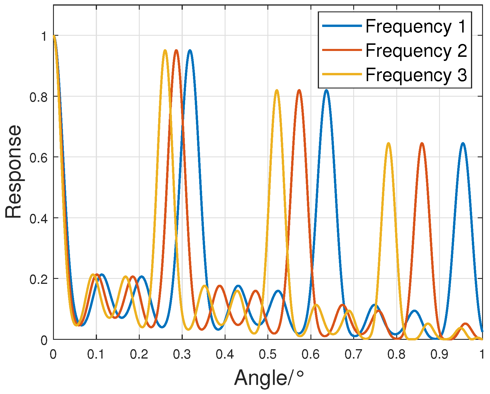
According to the proposed multi-subpulse jamming suppression scheme, the overall pattern response at each angle is the minimum value of the pattern responses across all frequency points, as expressed in (19).

$$\begin{array}{c}L\left({\theta }_j\right)=min{L}_n\left({\theta }_j\right)\hfill \\ \left\{\begin{array}{c}{L}_n\left({\theta }_j\right)={\left|\rho \left({\mathbf{d}}_{Gopt},f_n,{\theta }_j\right)\right|}^2{f}_n\in U=\left\{f_1,\cdots ,f_N\right\}\hfill \\ {\theta }_j\in \Phi \hfill \end{array}\right.\hfill \end{array}$$

(19)

N denotes the number of frequency points in the frequency set U, and $f_n$ denotes the n-th frequency point.

As shown in (19), for any given frequency set U, adding a new frequency point will always result in a PGLL that is less than or equal to the original PGLL. This paper proposes a stepwise subpulse frequency design scheme. Specifically, the PGLL is calculated for the current frequency set, and the angle corresponding to the PGLL is identified. A new frequency point is then searched within the frequency range to minimize the response at this angle, and the new frequency point is added to the current frequency set. This process is repeated until the PGLL approaches the PSO optimization results or the maximum number of subpulses is reached. The overall process of the proposed algorithm is shown in Algorithm 1.

Algorithm 1 Joint Optimization of Positions and Carrier Frequencies

1: for $k_1=1$ to $T_{outer}$ do   2:    Initialize the particle swarm ${\mathbf{D}}_{k1}$ (composed of particles $\mathbf{d}$) according to the constraints.   3:    if $k_1\ne 1$ then   4:      Incorporate the global best particle ${\mathbf{d}}_{k1-1}^{Opt}$ from the previous generation into the      particle swarm ${\mathbf{D}}_{k1}$.   5:    end if   6:    for $k_2=1$ to $T_{inner}$ do   7:      Calculate the fitness based on (13).   8:      Map ${\mathbf{D}}_{k_1}^{\left(k_2\right)}$ onto ${\mathbf{X}}_{k_1}^{\left(k_2\right)}$ based on (14).   9:      Update the velocity according to (17) and move ${\mathbf{X}}_{k_1}^{\left(k_2\right)}$ to obtain the updated ${\mathbf{X}}_{k_1}^{\left(k_2+1\right)}$      based on (18). 10:      Map ${\mathbf{X}}_{k_1}^{\left(k_2+1\right)}$ onto ${\mathbf{D}}_{k_1}^{\left(k_2+1\right)}$ based on (14). 11:    end for 12:    Save the global best particle ${\mathbf{d}}_{k1}^{Opt}$. 13: end for 14: Initialize the subpulse frequency set U with the minimum frequency point. 15: while $n\le N$ do 16:    Calculate the angle of the PGLL ${\theta }_n$ under the current subpulse frequency set U based    on the optimized radar positions ${\mathbf{d}}_{T_{outer}}^{Opt}$ and (19). 17:    Iterate through the frequency range to find $f_n$ that minimizes the response at ${\theta }_n$. 18:    Add $f_n$ to the subpulse frequency set U. 19: end while 20: return Optimized positions ${\mathbf{d}}_{T_{outer}}^{Opt}$ and frequency set U

3.3. Optimal Frequency Selection via SJNR Comparison

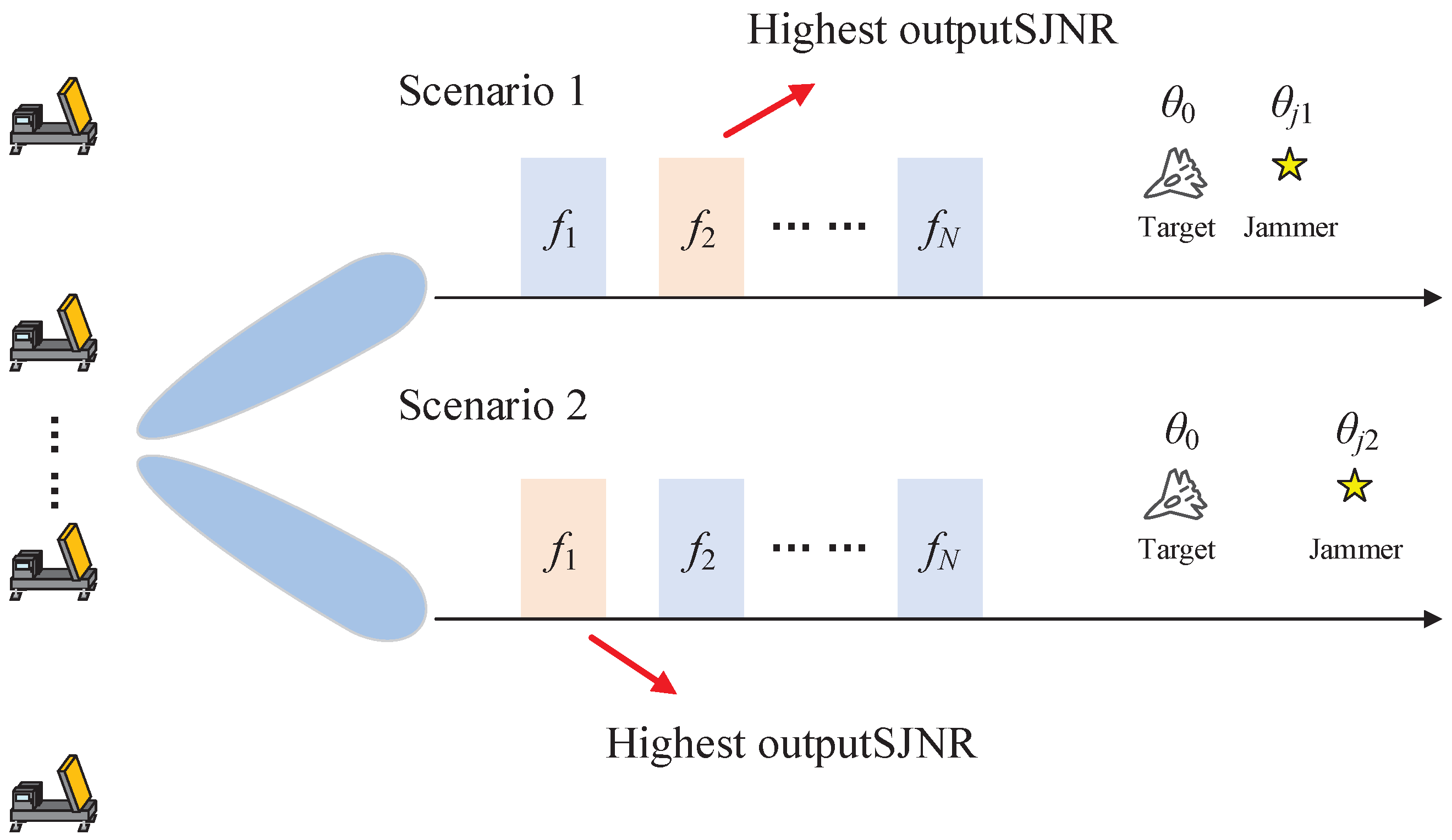
In practical applications, using multiple pulses with different frequencies can lead to challenges in achieving coherent accumulation across pulses. Consequently, continuously employing multiple sub-pulses may not be the optimal approach. In the proposed framework, after designing the radar position and carrier frequency, the optimal frequency under specific jamming scenarios (e.g., target-jammer angle separation) is uniquely determined. This motivates the development of a frequency selection strategy to identify the most performant frequency within the current scenario. Subsequent transmissions then focus exclusively on this single optimal frequency to avoid SNR loss caused by incoherent accumulation of signals with different carrier frequencies. This approach is illustrated in Figure 6.

The ultimate objective of optimization in this study is to enhance the output SJNR after jamming suppression. To achieve this, the following frequency selection strategy can be employed:

1. Sequentially transmit pulses at each frequency within the frequency set U. After jamming suppression for each pulse, record the corresponding output SJNR.

2. Select the carrier frequency with the highest recorded output SJNR as the operating frequency for subsequent pulse.

3. When the target and jammer continuously move in space, the output SJNR for the current carrier frequency may gradually degrade. If the output SJNR drops significantly relative to the initial value (e.g., a decline exceeding 3 dB), revert to step 1 to re-select the new optimal frequency.

This strategy avoids frequent switching of the operating frequency, thereby effectively reducing the complexity of the system and the difficulty of pulse accumulation.

4. Verification with Simulation

4.1. Validation of Effectiveness

This paper considers a distributed array radar system with one main radar and multiple auxiliary radars. The main radar transmits signals, while all radars receive signals. The system parameters are listed in

Table 1. Parameter of distributed array radar system.

Parameter	Value
Center frequency $f_c$	3 GHz
Number of auxiliary radars $M^{\prime }$	6
Baseline length l	120 m
Frequency variation range $\left[f_c-\Delta f,f_c+\Delta f\right]$	[2.7 GHz, 3.3 GHz]
Number of subarrays in main radar M	5
Main radar aperture	2 m

. In practice, the number of auxiliary radars is determined by the required number of spatial degrees of freedom, while the baseline length depends on the minimum angle between the target and the mainlobe jamming that needs to be suppressed. This is because the baseline length determines the spatial resolution of the distributed array radar system.

The algorithm parameters are shown in

Table 2. Parameter of the algorithm.

Parameter	Value
Outer iteration number $T_{outer}$	10
Inner iteration number $T_{inner}$	100
Minimum radar spacing $d_c$	2 m
Optimized angle range $\Phi$	0.05°∼1.5°
Step size of angular range	0.01°
Step size of frequency range	10 MHz
Number of particles	100
Maximum number of subpulses N	8
Cognitive learning factor $c_1$	0.1
Global learning factor $c_1$	0.1
Maximum inertia weight ${\omega }_{v max}$	0.9
Minimum inertia weight ${\omega }_{v min}$	0.4
Cognitive learning random $r_1$	0∼0.1
Global learning random $r_2$	0∼0.1

. The random numbers $r_1$ and $r_2$ follow a uniform distribution.

Figure 7 illustrates the convergence behavior of the fitness value, which stabilizes after approximately 250 iterations.

The fitness value corresponds to the PGLL in (13). After optimization, this value is −7.87 dB. The optimized radar positions are shown in

Table 3. Optimized Radar Positions.

Radar	Position (m)
Auxiliary Radar 1	0
Auxiliary Radar 2	19.58
Auxiliary Radar 3	43.48
Auxiliary Radar 4	62.89
Main Radar	76.84
Auxiliary Radar 5	99.79
Auxiliary Radar 6	120

.

The optimized radar positions are incorporated into the subpulse frequency optimization algorithm.Initialize the subpulse frequency set U with the minimum frequency 2.7 GHz. The optimized subpulse frequencies U are shown in

Table 4. Optimized Subpulse Carrier Frequencies.

Frequencies (GHz)
2.70	3.30	2.95	3.14	3.03	2.83

, and the responses of each frequency within the angular range are illustrated in Figure 8.

After processing with the algorithm, the PGLL has reached the optimization upper limit under the current radar positions using only six frequency points. Adding additional frequency points does not further reduce the PGLL. At this stage, the overall beam pattern, calculated by integrating the optimized radar positions and optimized frequencies using (19), is shown in Figure 9.

The final optimized PGLL is −7.95 dB, which is very close to the result obtained by the PSO algorithm. The slight discrepancy is primarily caused by the step size used in the angular range during the iterative process. Simulation shows that reducing the step size can further minimize this error; however, it significantly increases the computation time. The 0.01° step size adopted in this paper achieves a balance between accuracy and efficiency, delivering a nice optimization performance.

To demonstrate the effectiveness and performance advantages of the joint optimization method, the optimization results in this paper are compared with the results obtained by optimizing only the radar positions. The comparison is also shown in Figure 9.

Notably,

Table 5. Comparison of PGLL.

Proposed Method	CSSA	DSMA	WCA	QPSO	EHHO	AGA
−7.95 dB	−4.44 dB	−4.38 dB	−4.36 dB	−4.48 dB	−4.38 dB	−4.32 dB

presents the PGLL values for all algorithms shown in Figure 9. The proposed joint optimization method for radar positions and subpulse frequencies demonstrates better performance, achieving a lower PGLL value compared to the position-only optimization scheme. Algorithms employing the position-only optimization scheme achieve similar PGLL values, which indicates an inherent performance limit of this scheme in grating lobe suppression under the current parameter settings.

During the optimization process, the target at 0° was used as a fixed condition. As discussed earlier, when the target is located at other azimuth angles, the beam pattern is obtained by scaling the optimized pattern at 0°. Therefore, the optimized PGLL remains valid. Figure 10 presents a comparison of the beam patterns when the target is located at different angles.

Figure 10 demonstrates that optimizing for the target located at 0° simultaneously optimizes for scenarios where the target is located at other angles.

4.2. Mainlobe Jamming Suppression Performance Verification

According to (9), a lower PGLL indicates a smaller SJNR loss after mainlobe jamming suppression, which implies that the proposed method offers better mainlobe jamming suppression performance. To validate this theory, signal-level simulations are used for verification. The signal parameters are shown in

Table 6. Signal Parameters.

Parameter	Value
Target signal SNR	≈18 dB
Barrage jamming JNR	≈40 dB
Target angle	$0^{\circ }$
Jamming signal angle range	$0^{\circ }$∼$1.5^{\circ }$

. Both the SNR and JNR represent the values obtained after full-array beamforming in the distributed array radar. Since noise and jamming signals are random signals, the values obtained from the actual signal statistics may have small fluctuations.

Two beamforming algorithms, minimum variance distortionless response (MVDR) [29] and minimum mean squared error (MMSE) [36], are applied to calculate the weights for mainlobe jamming suppression. The calculation method of MVDR is shown in (2), and the method for MMSE is presented in (20).

$${\mathbf{w}}_{\mathrm{MMSE}}={\mathbf{R}}_{\mathrm{A}}^{-1}{\mathbf{r}}_{\mathrm{AM}}$$

(20)

${\mathbf{R}}_{\mathrm{A}}$ denotes the covariance matrix of the auxiliary radar signals, and ${\mathbf{r}}_{\mathrm{AM}}$ represents the cross-covariance matrix between the auxiliary and main radar signals. By applying ${\mathbf{w}}_{\mathrm{MMSE}}$ to weight the auxiliary radar signals and subtracting the weighted result from the main radar signal, jamming suppression is achieved.

The other parameters are the same as those in the previous subsection. The resulting output SJNRs are shown in Figure 11.

Figure 11 demonstrates that the proposed joint optimization algorithm for radar positions and carrier frequencies achieves substantial performance improvements in mainlobe jamming suppression for both beamformers. As shown in

Table 7. Minimum output SJNR (Target at $0^{\circ }$).

Beamformer	Proposed Method	CSSA	DSMA	WCA	QPSO	EHHO	AGA
MVDR	16.87 dB	14.26 dB	14.24 dB	13.98 dB	14.03 dB	14.19 dB	14.24 dB
MMSE	13.07 dB	10.19 dB	9.50 dB	9.26 dB	9.97 dB	8.68 dB	9.53 dB

, these improvements are quantified using the minimum output SJNR over the entire mainlobe region as the comparative metric.

As discussed before, the core principle of anti-mainlobe jamming in distributed array radar lies in converting the mainlobe jamming of the main radar into sidelobe jamming for the entire array by increasing the baseline length. This mechanism requires that the mainlobe jamming of the main radar remain outside the main beam of the distributed array radar. In other words, when the beam is steered toward the target, the jamming must lie beyond the first null of the entire array’s beam pattern, as approximately characterized by the following equation.

$$\Delta \theta \ge arcsin\left({\displaystyle \frac{\lambda }{l}}\right)\approx {\displaystyle \frac{\lambda }{l}}$$

(21)

$\Delta \theta$ represents the angle between the jamming and the target.

The simulations in the paper also validate this point. Figure 9 shows that the first null of the beam pattern optimized by the proposed algorithm is approximately 0.05°, and Figure 11a demonstrates that the anti-jamming performance of the proposed method begins to degrade rapidly when the angle between the jamming and target is less than 0.05°.

It is worth noting that the optimization objective of the proposed method in this study is PGLL. This implies that the proposed algorithm does not necessarily outperform the position-only optimization method at all angles; instead, it ensures a lower overall grating lobe level. This is also evident from the results in Figure 9. While the traditional method may exhibit comparable or slightly better jamming suppression performance at a few specific angles, the proposed algorithm demonstrates a significant advantage when considering the entire mainlobe angular range.

Under the same parameter settings except that the target angle is set to ${40}^{\circ }$ and the jamming angle is varied within the range of ${40}^{\circ }$∼$41.5^{\circ }$, the resulting output SJNRs are shown in Figure 12.

As the azimuth angle increases, the proposed method maintains a relatively stable output SJNR. The minimum output SJNR over the entire mainlobe region is shown in

Table 8. Minimum output SJNR (Target at ${40}^{\circ }$).

Beamformer	Proposed Method	CSSA	DSMA	WCA	QPSO	EHHO	AGA
MVDR	16.92 dB	12.83 dB	13.53 dB	13.48 dB	13.30 dB	14.78 dB	13.90 dB
MMSE	12.42 dB	9.83 dB	8.11 dB	7.12 dB	7.34 dB	8.35 dB	7.49 dB

.

This demonstrates the effectiveness of the optimization method when the target and jamming angles vary.

4.3. Dynamic Jamming Scenario

As discussed in Section 3.3, in the proposed optimization framework, the optimal frequency in a given scenario is unique. By selecting one of the frequencies based on the anti-jamming performance of different pulses, frequent switching of carrier frequencies can be avoided. To validate this approach, a dynamic anti-jamming scenario is designed in this subsection, as illustrated in Figure 13. Pulse repetition time (PRT) is 1ms, and other parameters are the same as those in the previous subsection.

First, the pulse signals at each frequency in the optimized frequency set are sequentially transmitted. Jamming suppression is then performed individually for each pulse, and the corresponding SJNR is calculated. The frequency associated with the highest output SJNR is selected as the optimal frequency, and this frequency is continuously used for subsequent pulse.

Jamming suppression performance in the dynamic jamming scenario is shown in Figure 14.

As shown in Figure 14, during the initial pulses, the proposed anti-jamming architecture tests different frequencies for jamming suppression. Evidently, the jamming suppression performance varies significantly across carrier frequencies, with some frequencies exhibiting inferior performance. However, after comparing the output SJNR, the optimal carrier frequency is selected. Subsequent pulses maintain stable anti-jamming performance, consistently outperforming the method that only optimizes positions.

The results demonstrate that the proposed optimization yields multiple distinct carrier frequencies, and selecting one of them in a specific scenario is feasible.

5. Conclusions

Radar systems are facing increasingly severe electronic jamming threats, with jamming techniques becoming more complex and diverse. To enhance electronic countermeasure capabilities, radar systems must adopt new “increments.” Distributed array radar introduces multiple auxiliary radars to transform mainlobe jamming on the main radar into sidelobe jamming for the entire array, effectively improving the system’s detection capability under mainlobe jamming conditions. However, the grating lobe problem caused by long baselines can degrade mainlobe jamming suppression performance in certain angular ranges. Building on the position design of distributed array radar, this paper introduced the frequency parameter as a new “increment” by employing multiple subpulses with different frequencies to enhance jamming suppression performance. A joint optimization scheme was introduced, along with a new optimization function and framework. Subsequently, an optimal carrier frequency selection was developed based on the comparison of output SJNR, enhancing the implementation feasibility of the optimization framework. Both model-based simulations and signal-level simulations have validated the effectiveness of the proposed optimization method. Compared to the position-only optimization scheme, the proposed method reduces grating lobe by more than 3 dB and improves the output SJNR by nearly 3 dB. While the current model was primarily designed for single mainlobe jamming scenarios, the joint optimization of carrier frequency and location could still theoretically enhance performance in multi-mainlobe jamming environments, which we will further explore in future work. This work provides a reference for the design of position and frequency configurations in distributed array radar systems for practical applications, aiming to enhance the spatial mainlobe jamming suppression performance.

References

1. Sun, Z.; Quan, Y.; Liu, Z. A Non-Uniform Interrupted-Sampling Repeater Jamming Method for Intra-Pulse Frequency Agile Radar. Remote Sens. 2023, 15, 1851. [Google Scholar] [CrossRef]
2. Wei, S.; Fang, Y.; Song, Y.; Wei, S.; Zhang, L. Joint Jam Perception and Adaptive Waveform Optimization for Anti-Interrupted Sampling Repeater Jamming. IEEE Trans. Aerosp. Electron. Syst. 2024, 60, 1129–1147. [Google Scholar] [CrossRef]
3. Vendik, O.G.; Kozlov, D.S. Phased Antenna Array With a Sidelobe Cancellation for Suppression of Jamming. IEEE Antennas Wirel. Propag. Lett. 2012, 11, 648–650. [Google Scholar] [CrossRef]
4. Pan, B.; Dong, L.; Yu, X.; Yao, X.; Sha, M.; Cui, G. Joint Polarization-Space-Time Processing for Mainlobe Jamming via CP Decomposition. IEEE Sens. J. 2023, 23, 14781–14794. [Google Scholar] [CrossRef]
5. Zhao, Y.; Wu, J.; Zhang, L. A Novel Robust Digital Subarray Partition Algorithm With Binary Coding. IEEE Trans. Antennas Propag. 2023, 71, 6126–6131. [Google Scholar] [CrossRef]
6. Xiao, G.; Quan, Y.; Sun, Z.; Wen, B.; Liao, G. Design of a Digital Array Signal Processing System with Full Array Element. Remote Sens. 2023, 15, 4043. [Google Scholar] [CrossRef]
7. Yang, X.; Li, Y.; Liu, F.; Lan, T.; Long, T.; Sarkar, T.K. Robust Adaptive Beamforming Based on Covariance Matrix Reconstruction With Annular Uncertainty Set and Vector Space Projection. IEEE Antennas Wirel. Propag. Lett. 2021, 20, 130–134. [Google Scholar] [CrossRef]
8. Guo, L.; Deng, W.; Yao, D.; Yang, Q.; Ye, L.; Zhang, X. A Knowledge-Based Auxiliary Channel STAP for Target Detection in Shipborne HFSWR. Remote Sens. 2021, 13, 621. [Google Scholar] [CrossRef]
9. Ge, M.; Cui, G.; Yu, X.; Kong, L. Mainlobe jamming suppression with polarimetric multi-channel radar via independent component analysis. Digit. Signal Process. 2020, 106, 102806. [Google Scholar] [CrossRef]
10. Ma, X.; Jiang, S.; Zhang, S.; Zhang, R.; Sheng, W. Joint Wideband Beamforming Algorithm for Main Lobe Jamming Suppression in Distributed Array Radar. Remote Sens. 2024, 16, 2402. [Google Scholar] [CrossRef]
11. Hu, L.; Wu, J.; Zhang, L. Airborne distributed array position calibration using sparse spatial-frequency accompanying flight MISO array. AEU-Int. J. Electron. Commun. 2024, 178, 155203. [Google Scholar] [CrossRef]
12. Yang, C.; Yi, W.; Champagne, B. Joint Antenna Selection and Beamforming for Area Surveillance with Spatially Distributed Array Radar. IEEE Trans. Aerosp. Electron. Syst. 2024, 61, 2899–2913. [Google Scholar] [CrossRef]
13. Han, B.; Qu, X.; Yang, X.; Zhang, Z.; Li, W. DRFM Repeater Jamming Suppression Method Based on Joint Range-Angle Sparse Recovery and Beamforming for Distributed Array Radar. Remote Sens. 2023, 15, 3449. [Google Scholar] [CrossRef]
14. Yu, H.; Liu, N.; Zhang, L.; Li, Q.; Zhang, J.; Tang, S.; Zhao, S. An Interference Suppression Method for Multistatic Radar Based on Noise Subspace Projection. IEEE Sens. J. 2020, 20, 8797–8805. [Google Scholar] [CrossRef]
15. Yang, X.; Yin, P.; Zeng, T.; Sarkar, T.K. Applying Auxiliary Array to Suppress Mainlobe Interference for Ground-Based Radar. IEEE Antennas Wirel. Propag. Lett. 2013, 12, 433–436. [Google Scholar] [CrossRef]
16. Wang, C.; Zheng, Z.; Zhang, K.; Chang, S.; Liu, Q. Adaptive Main-Lobe Jamming Suppression Based on Cascaded LMS Filter With Low-Cost Distributed Radar. IEEE Sens. J. 2023, 23, 26292–26301. [Google Scholar] [CrossRef]
17. Chen, X.; Shu, T.; Yu, K.B.; Zhang, Y.; Lei, Z.; He, J.; Yu, W. Implementation of an Adaptive Wideband Digital Array Radar Processor Using Subbanding for Enhanced Jamming Cancellation. IEEE Trans. Aerosp. Electron. Syst. 2021, 57, 762–775. [Google Scholar] [CrossRef]
18. Pu, W.; Liang, Z.; Wu, J.; Liu, Q. Joint Generalized Inner Product Method for Main Lobe Jamming Suppression in Distributed Array Radar. IEEE Trans. Aerosp. Electron. Syst. 2023, 59, 6940–6953. [Google Scholar] [CrossRef]
19. Tian, X.; Wang, B.; Tao, K.; Li, K. An Improved Synthesis of Sparse Planar Arrays Using Density-Weighted Method and Chaos Sparrow Search Algorithm. IEEE Trans. Antennas Propag. 2023, 71, 4339–4349. [Google Scholar] [CrossRef]
20. Zhu, W.; Wei, Z.; Xiang, Y.; Chai, X.; Liu, S.; Fan, G.; Zhang, H.; Zhang, H.; Qi, W. Sparse Optimal Design of an Ultrasonic Sensor Array for Fast TFM Based on a Discrete Slime Mold Algorithm. IEEE Sens. J. 2024, 24, 12207–12216. [Google Scholar] [CrossRef]
21. Xu, Y.; Wang, D.; Wang, A.; Yan, Y. WCA-Based Low-PSLL and Wide-Nulling Beampattern Synthesis for Radar Applications. Remote Sens. 2022, 14, 4204. [Google Scholar] [CrossRef]
22. Liu, Y.; Huang, L.; Xie, X.; Ye, H. A Hybrid Optimization Algorithm for the Synthesis of Sparse Array Pattern Diagrams. Appl. Sci. 2025, 15, 6490. [Google Scholar] [CrossRef]
23. Li, T.; Liu, Z.; Zhang, C.; Cheng, F.; Yao, Y.; Li, X.; He, H.; Yang, Y. Synthesis of Non-Uniform Spiral Antenna with Low Peak Sidelobe Level Using Enhanced Harris Hawks Optimization Algorithm. Electronics 2024, 13, 2959. [Google Scholar] [CrossRef]
24. Yang, X.; Li, Y.; Liu, F.; Lan, T.; Teng, L.; Sarkar, T.K. Antenna position optimization method based on adaptive genetic algorithm with self-supervised differential operator for distributed coherent aperture radar. IET Radar Sonar Navig. 2021, 15, 677–685. [Google Scholar] [CrossRef]
25. Huang, J.Y.; Liu, C.Y.; Hu, W.; Liao, K. Design of a Grating Lobes-Free Architecture for Distributed Sensor System with Arbitrary Element Spacing. Remote Sens. 2022, 14, 1356. [Google Scholar] [CrossRef]
26. Tian, D.; Wang, C.; Ren, W.; Liang, Z.; Liu, Q. ECCM Scheme for Countering Main-Lobe Interrupted Sampling Repeater Jamming via Signal Reconstruction and Mismatched Filtering. IEEE Sensors J. 2023, 23, 13261–13271. [Google Scholar] [CrossRef]
27. Lu, L.; Gao, M. A Truncated Matched Filter Method for Interrupted Sampling Repeater Jamming Suppression Based on Jamming Reconstruction. Remote Sens. 2022, 14, 97. [Google Scholar] [CrossRef]
28. Liu, Z.; Quan, Y.; Wu, Y.; Xu, K.; Xing, M. Range and Doppler reconstruction for sparse frequency agile linear frequency modulation-orthogonal frequency division multiplexing radar. IET Radar Sonar Navig. 2022, 16, 1014–1025. [Google Scholar] [CrossRef]
29. Huang, Y.; Zhou, M.; Vorobyov, S.A. New Designs on MVDR Robust Adaptive Beamforming Based on Optimal Steering Vector Estimation. IEEE Trans. Signal Process. 2019, 67, 3624–3638. [Google Scholar] [CrossRef]
30. Chen, J.; Zhao, L.; Jiang, M.; Wu, Z. Sherman-Morrison Formula Aided Adaptive Channel Estimation for Underwater Visible Light Communication With Fractionally-Sampled OFDM. IEEE Trans. Signal Process. 2020, 68, 2784–2798. [Google Scholar] [CrossRef]
31. Long, X.; Li, K.; Tian, J.; Wang, J.; Wu, S. Ambiguity Function Analysis of Random Frequency and PRI Agile Signals. IEEE Trans. Aerosp. Electron. Syst. 2021, 57, 382–396. [Google Scholar] [CrossRef]
32. Fang, Y.; Zhang, L.; Wei, S.; Wang, T.; Wu, J. Online Frequency-Agile Strategy for Radar Detection Based on Constrained Combinatorial Nonstationary Bandit. IEEE Trans. Aerosp. Electron. Syst. 2023, 59, 1693–1706. [Google Scholar] [CrossRef]
33. Sun, J.; Yuan, Y.; Greco, M.S.; Gini, F.; Yang, X.; Yi, W. Anti-deception Jamming Resource Scheduling for Multi-target Tracking in Distributed Radar Networks. IEEE Trans. Aerosp. Electron. Syst. 2024, 60, 9111–9128. [Google Scholar] [CrossRef]
34. Clerc, M.; Kennedy, J. The particle swarm—explosion, stability, and convergence in a multidimensional complex space. IEEE Trans. Evol. Comput. 2002, 6, 58–73. [Google Scholar] [CrossRef]
35. Shi, Y.; Eberhart, R. A modified particle swarm optimizer. In Proceedings of the 1998 IEEE International Conference on Evolutionary Computation Proceedings, IEEE World Congress on Computational Intelligence (Cat. No.98TH8360), Anchorage, AK, USA, 4–9 May 1998; pp. 69–73. [Google Scholar] [CrossRef]
36. Guo, Y.; Zhang, L.; Zhang, J.; Guo, P.; Chen, Z. A coherent signal beamforming technique based on sub-array cross correlation. Digit. Signal Process. 2022, 121, 103291. [Google Scholar] [CrossRef]
Figure 1. Schematic diagram of the distributed array radar.
Remotesensing 17 02423 g001
Figure 2. Multi-frequency jamming suppression diagram.
Remotesensing 17 02423 g002
Figure 3. Illustration of beam pattern scaling effect caused by carrier frequency variation.
Remotesensing 17 02423 g003
Figure 4. Constrained particle generation.
Remotesensing 17 02423 g004
Figure 5. Angular range corresponding to the frequency range.
Remotesensing 17 02423 g005
Figure 6. Optimal frequency selection diagram.
Remotesensing 17 02423 g006
Figure 7. The variation of PGLL with the number of iterations.
Remotesensing 17 02423 g007
Figure 8. The responses of optimized frequencies.
Remotesensing 17 02423 g008
Figure 9. Comparison of beam pattern.
Remotesensing 17 02423 g009
Figure 10. Impact of target angle variation.
Remotesensing 17 02423 g010
Figure 11. Mainlobe jamming suppression performance (target at 0 ).
Remotesensing 17 02423 g011
Figure 12. Mainlobe jamming suppression performance (target at 40 ).
Remotesensing 17 02423 g012
Figure 13. Dynamic jamming scenario diagram.
Remotesensing 17 02423 g013
Figure 14. Dynamic jamming scenario performance.
Remotesensing 17 02423 g014