Scattering Center Prior-Guided Diffusion for Unknown-Azimuth SAR Image Generation

Highlights

What are the main findings?

• A PSF-constrained ISTA method is used to extract dominant scattering centers from known-view SAR images.
• A scattering center guided conditional diffusion model improves unseen-azimuth SAR image generation over a GAN baseline.

What are the implications of the main findings?

• Scattering center priors provide effective physical guidance for SAR image generation under sparse angular sampling.
• This framework provides a novel and practical solution for physics-guided unseen-azimuth SAR image generation under few-shot conditions.

Abstract

Generating synthetic aperture radar (SAR) images at unknown azimuth angles under limited sample conditions remains a challenging task, since target scattering characteristics vary significantly with observation angle and are difficult to model effectively using only image-domain priors. To address this issue, this paper proposes a scattering center prior-guided conditional diffusion framework for unknown-azimuth SAR image generation. First, the Iterative Shrinkage–Thresholding Algorithm (ISTA) constrained by the Point Spread Function (PSF) is employed to extract dominant scattering centers from SAR images at known viewing angles, obtaining sparse and physically interpretable scattering center maps. Subsequently, the target category, azimuth angle, and scattering map are jointly used as conditional vector inputs to train the diffusion model. During the inference stage, scattering maps from known azimuth angles are fused to construct a scattering prior for the unknown azimuth, which is used to guide the generation of the corresponding SAR image. Experimental results under sparse angular sampling conditions demonstrate that, compared with the scattering-guided GAN baseline and the non-learning image-domain interpolation baseline, the proposed method better preserves dominant scattering structures and generates unknown-azimuth SAR images with clearer target contours, more stable strong scattering regions, and fewer local artifacts. In summary, introducing dominant scattering center priors into the conditional diffusion model provides effective physical constraints for SAR image generation and improves unseen-azimuth SAR image generation under the evaluated sparse angular sampling conditions.

1. Introduction

Synthetic aperture radar (SAR) is capable of providing all-weather and all-day imaging and can reliably acquire high-resolution images of ground and maritime targets under challenging environmental conditions, such as cloud cover, fog, and low-illumination scenes. Owing to these advantages, SAR has been widely employed in a variety of applications, including maritime target surveillance, battlefield situation awareness, disaster assessment, and resource exploration. With the rapid advancement of deep learning techniques, intelligent SAR image interpretation has attracted increasing attention in recent years [1,2]. However, the performance of deep learning-based methods is highly dependent on the availability of large-scale and diverse training data. In practical applications, it is extremely difficult to construct large-scale SAR target datasets covering full azimuth and elevation angles, due to the constraints of satellite or airborne platform trajectories, the strict requirements of observation geometry and imaging conditions, and the high cost of data acquisition [3,4,5,6]. As a result, the scarcity of multi-aspect SAR data has become a critical factor limiting the generalization capability and robustness of intelligent SAR image interpretation methods in complex and dynamic observation scenarios.

Compared with optical imaging, SAR imaging involves a substantially more complex physical mechanism and exhibits fundamental differences in image formation. Specifically, SAR echoes are jointly determined by electromagnetic scattering characteristics, target geometry, material properties, and the imaging and observation angles [7,8]. Meanwhile, SAR images are inherently affected by speckle noise and sidelobe interference, causing the scattering center distribution, scattering intensity, and shadow characteristics of the same target to vary nonlinearly with the observation aspect [9,10,11]. Therefore, conventional optical image augmentation strategies, such as translation, rotation, flipping, and interpolation, are generally incapable of preserving the underlying physical laws of SAR imaging, and the generated samples often suffer from evident physical inconsistency [12]. Accordingly, it is of great significance to develop an intelligent generative framework that can extract physically informative features from SAR data acquired at known viewing angles and further infer highly reliable cross-view samples, thereby alleviating the incompleteness of training data for SAR target recognition.

In recent years, generative methods represented by generative adversarial networks (GANs) [13,14] and diffusion models [15,16,17] have provided new perspectives for SAR image generation and data augmentation. In early studies, GAN-based methods learned the data distribution through adversarial training between a generator and a discriminator, offering advantages such as fast generation speed and flexible conditional control. However, their training process is often unstable, and under limited sample conditions, they are prone to mode collapse, background distortion, and degraded generation fidelity. Diffusion models learn the data distribution through a progressive noising and reverse denoising process, and generally exhibit superior training stability, higher generation quality, and better distribution coverage. Nevertheless, their drawbacks include a large number of iterative sampling steps and high inference cost, while they are also more sensitive to computational resources and the quality of training data.

Despite these encouraging advances, existing methods still exhibit several limitations for the task of generating SAR images at unseen azimuth angles under small-sample conditions. First, many existing approaches still perform conditional modeling primarily in the image domain, while insufficient attention has been paid to incorporating physical prior knowledge, such as the dominant scattering structures of the target and their variation patterns with observation angle, into the generative process so as to faithfully preserve the scattering center distribution under different aspects. Second, in the absence of complete three-dimensional geometry and accurate electromagnetic parameters, it remains an open problem how to exploit only the interpretable scattering center structures contained in SAR images acquired at limited known angles to construct a stable and transferable physical prior representation for unseen view generation.

To address the above challenges, this paper focuses on the generation of SAR images at unseen azimuth angles and proposes a scattering center prior-guided generative framework. The key motivation is that unseen-azimuth SAR image generation is not merely an image generation problem, but also a scattering structure inference problem. Due to the aspect-dependent electromagnetic scattering characteristics of SAR targets, the dominant scattering centers may vary with the observation azimuth. Therefore, generative models that rely only on image-domain conditional control may learn the global image distribution, but they can still produce inconsistent scattering structures, or physically implausible target details under sparse-view conditions.

To introduce physically interpretable structural guidance into the generation process, an iterative shrinkage–thresholding algorithm (ISTA) [18] constrained by the point spread function (PSF) is first employed to extract dominant scattering centers from SAR images acquired at known azimuths [19,20]. In this way, the SAR image is transformed into a sparse intermediate representation that is more consistent with the SAR imaging mechanism. Then, the SAR images at known azimuths and their corresponding scattering center representations are jointly used for generative model training, enabling the network to learn both image-domain texture distributions and scattering-structure distributions. Furthermore, scattering centers from multiple neighboring known azimuths are fused to construct a scattering-center position response prior for the target unseen azimuth, which is subsequently used to constrain the generation of scattering centers and the corresponding SAR images.

Compared with generative methods relying solely on image-domain conditional control, the proposed strategy offers two major advantages. On the one hand, the PSF-constrained ISTA method provides an interpretable pathway for extracting dominant scattering structures. On the other hand, the fusion of multi-aspect scattering centers introduces an intermediate constraint that is more consistent with electromagnetic scattering laws for unknown-view inference, and thus has the potential to improve structural fidelity, angular consistency, and the utility of the generated data for downstream recognition tasks.

In line with the recent trend of physics-guided generation, the proposed method can be regarded as an attempt to bridge traditional scattering mechanism modeling and modern generative models. The main novelty lies in the construction of a physics-guided SAR generation pipeline that explicitly connects sparse scattering-center reconstruction with conditional diffusion-based image generation.

The main contributions of this paper are summarized as follows.

1.

A PSF-constrained ISTA-based scattering center extraction method is proposed to obtain sparse and physically interpretable scattering center representations from known-azimuth SAR images, providing explicit physical priors for subsequent unseen-azimuth SAR image generation.

2.

A scattering center prior-guided framework for unknown-azimuth SAR image generation is constructed. By fusing the dominant scattering centers extracted from known observation angles, a scattering prior for unknown azimuth angles is established, enabling high-fidelity SAR image generation under unknown viewing conditions.

3.

Both simulated and measured datasets are established, and the effectiveness of the proposed method for unknown-angle SAR image generation under small-sample conditions is validated under different sparse sampling settings.

2. Related Work

2.1. Physics-Based SAR Image Simulation Methods

Traditional physics-based SAR image simulation methods can be broadly divided into three categories.

The first category involves parametric modeling based on Point Scattering Centers (PSCs), which aims to approximate the target response using a few dominant scattering structures. Early work by Holtzman et al. [21] introduced point scattering-based radar image simulation methods. Subsequently, Franceschetti et al. [22] developed SARAS, a raw SAR signal simulation approach designed for extended 3D scenes. Potter et al. [23] established a parametric modeling framework for SAR scattering centers, shifting the description of target scattering characteristics from mere pixel appearances to physically interpretable sparse intermediate representations. In particular, Potter and Moses formalized the Attributed Scattering Center (ASC) representation, in which a small number of scattering centers with physical attributes are used to characterize target signatures in a sparse and interpretable manner [24]. Furthermore, Akyildiz and Moses et al. [25] introduced a high-frequency scattering center model for SAR imagery, focusing on preserving dominant scattering terms to explain the primary scattering structures within an image.

The second category comprises high-frequency electromagnetic (EM) approximation methods, including Physical Optics (PO), Geometric Optics (GO) [26], the Geometric/Physical Theory of Diffraction (GTD/PTD), and Shooting and Bouncing Rays (SBR) [27]. Chang et al. [28] proposed a database-building methodology that integrates sensor orbital information, target geometry, Radar Cross Section (RCS), echo generation, and focus imaging. In this approach, target RCS is computed using a hybrid PO+PTD+SBR algorithm. Although high-frequency methods offer relatively high computational efficiency, their simulation accuracy is often compromised by the varying degrees of simplification applied to the underlying computational models.

The third category consists of full-wave methods and echo-level simulation techniques, which focus on the precise physical simulation of target echo signals. Representative full-wave solvers include the finite difference time domain (FDTD) method and the method of moments (MoM) [29,30]. In practical SAR simulation, tools such as RaySAR, CohRaS [31], SARViz [32], and FEKO [33] have also been used to support different levels of EM or image simulation, depending on the modeling assumptions and target scenarios.

Collectively, these methods follow a SAR simulation paradigm rooted in electromagnetic scattering mechanisms. Their core principle is to perform forward modeling of the target’s scattering response or SAR echo formation by integrating the target’s 3D geometry, observation imaging geometry, and EM scattering laws. While these traditional methods offer strong physical interpretability and can realistically characterize EM scattering mechanisms, they typically face significant bottlenecks, including prohibitive computational costs, heavy reliance on high-fidelity 3D CAD models and material parameters, and limited efficiency for large-scale batch generation.

2.2. Deep Unfolding Networks for Sparse Reconstruction

Deep unfolding networks have recently attracted increasing attention in inverse problems and sparse reconstruction. These methods unfold traditional iterative optimization algorithms, such as ISTA, ADMM, or AMP, into trainable neural network architectures by mapping each iteration to one network stage. Compared with purely data-driven networks, deep unfolding methods retain a certain degree of model interpretability by embedding optimization structures into neural networks.

Although deep unfolding networks can accelerate iterative sparse reconstruction by learning parameters such as step sizes, thresholds, and transform operators, this work adopts traditional PSF-constrained ISTA for scattering-center extraction. The objective of the ISTA module is not to obtain an end-to-end learned reconstruction result, but to construct a physically interpretable scattering-center prior for guiding the diffusion model. Traditional ISTA directly incorporates the SAR imaging PSF and sparsity constraint, which makes the extracted prior more transparent and reproducible. Moreover, deep unfolding variants introduce additional learnable parameters and require task-specific training, which introduces additional model complexity and training uncertainty. Therefore, a training-free PSF-constrained ISTA module is adopted to provide stable and physically constrained scattering center priors for the subsequent conditional diffusion model.

2.3. Deep Learning-Based SAR Image Generation

With the rapid development of deep generative models, SAR image generation has increasingly shifted from traditional electromagnetic simulation toward data-driven synthesis frameworks, such as Generative Adversarial Networks (GANs) and diffusion models. These technologies offer promising alternatives to overcome the bottlenecks of traditional electromagnetic (EM) simulations and achieve efficient SAR image synthesis.

Initial research primarily centered on GANs to model SAR image distributions for data augmentation, aiming to mitigate the performance degradation of Automatic Target Recognition (ATR) systems caused by data scarcity [5,34]. For instance, Cui et al. [35] proposed a WGAN-GP-based framework with an additional screening mechanism to improve azimuth-related controllability and mitigate mode collapse. Building on this, conditional GANs (cGANs) were employed to introduce constraints such as category and pose, enabling the generation of SAR samples with specific attributes. Feng et al. [36] established a mathematical model to map the nonlinear relationship between latent codes in InfoGAN and specific SAR image attributes, achieving precise numerical control and editing of the generated images. Furthermore, Wang et al. developed an azimuth controllable GAN consisting of a generator, a similarity discriminator, and an azimuth predictor, which synthesizes realistic SAR targets with specific intermediate angles by fusing features from two input images.

Concurrently, diffusion models have been introduced to SAR image synthesis due to their superior training stability and mode coverage and have shown strong potential in both conditional and unconditional SAR generation settings. To address the limitation that pure image-domain methods often overlook SAR electromagnetic scattering mechanisms, researchers have begun integrating 3D representations, geometric priors, and physical consistency constraints into generative frameworks [37,38]. Lei et al. [39] proposed SAR-NeRF, which combines traditional SAR imaging principles with Neural Radiance Fields (NeRF) to achieve implicit multi-view SAR representation by learning the attenuation coefficients and scattering intensity distributions within a 3D volume. Zhang et al. [40] introduced a physics-inspired GAN that incorporates the Ideal Point Scattering Center (PSC) model and physical consistency losses, effectively generating high-fidelity SAR images that adhere to physical laws under limited data conditions. More recently, Zhang et al. [41] developed GeoDiff-SAR, which leverages geometric point cloud priors and diffusion models to enhance the realism and azimuth-controllability of generated images, particularly for unknown viewing angles.

3. Materialsand Methods

3.1. Overall Framework

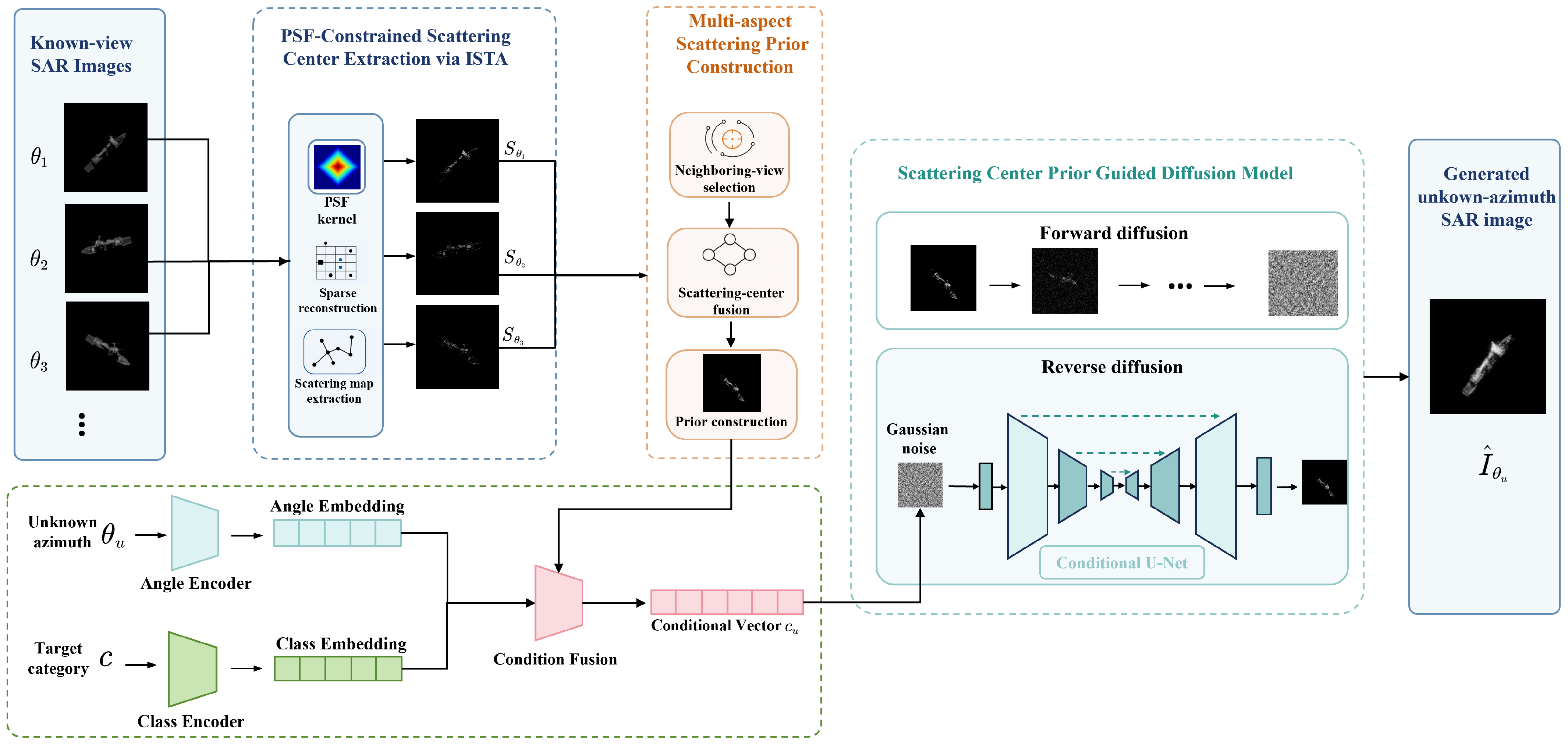
This paper proposes a physics-constrained generative framework for SAR image synthesis at unknown azimuth angles under limited data conditions, as illustrated in Figure 1. First, for SAR images with known azimuth angles, the Iterative Shrinkage–Thresholding Algorithm (ISTA) under Point Spread Function (PSF) constraints is utilized to extract the dominant scattering centers (DSCs). This process yields a sparse representation that is both physically interpretable and representative of the target’s electromagnetic characteristics. Second, during the training stage, a multi-conditional diffusion model is constructed. The network is trained by injecting joint conditions—including the observation angle, target category, and the extracted DSCs—to learn the underlying mapping between observation geometry, semantic attributes, image texture distribution, and dominant scattering structures. Finally, in the inference stage for small-sample scenarios, the DSCs extracted from multiple known azimuths are fused to construct a scattering center prior for the desired unknown azimuth. This prior, combined with the target angle and category, guides the diffusion model to generate high-fidelity, mechanism-consistent SAR images.

By utilizing DSCs as a bridge between the SAR imaging mechanism and deep generative models, the proposed method explicitly incorporates physical structural constraints into the generation process. By incorporating dominant scattering center priors, the proposed method provides additional structural guidance for unseen-azimuth interpolation under the evaluated sparse angular sampling conditions.

3.2. PSF-Constrained Scattering Center Extraction via ISTA

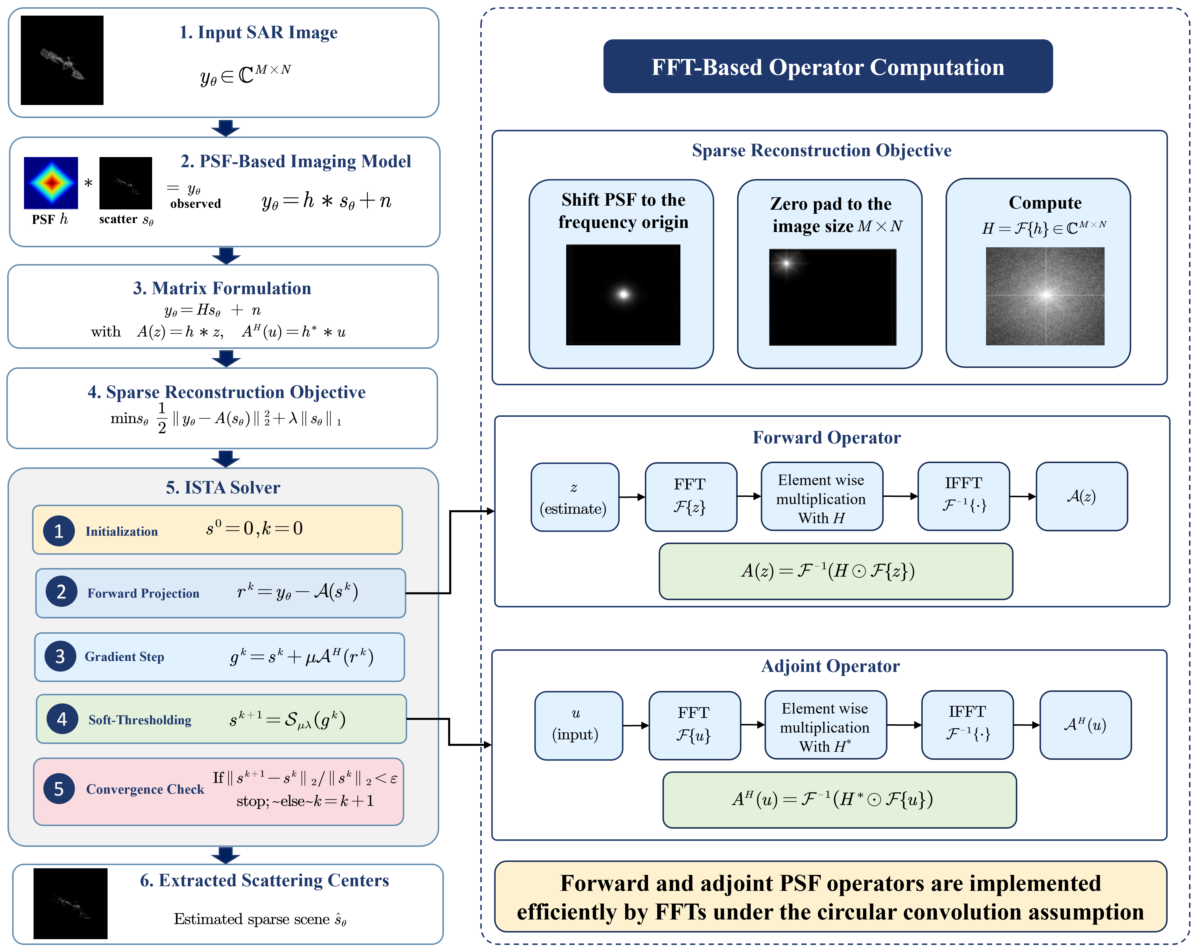
The extraction of scattering centers can be equivalently formulated as the estimation of scattering center parameters from SAR observations based on a parametric scattering center model. The process of PSF-constrained scattering center extraction via ISTA is illustrated in Figure 2. According to the PO and GTD, the Attributed Scattering Center (ASC) model of a target can be represented as:

$$S(f,\phi )={\displaystyle \sum _{i=1}^M}{A}_i·{\left({\displaystyle \frac{f}{f_0}}\right)}^{{\alpha }_i}·exp\left[-j4\pi {\displaystyle \frac{f}{c}}(x_{i}cos\phi +y_{i}sin\phi )\right]$$

(1)

It can be observed from the above formulation that the scattering characteristics of a target can be accurately approximated by the vector superposition of several dominant scattering centers located at specific positions. In high-resolution SAR imagery, the target echo is typically dominated by a limited number of prominent scattering structures, and the resulting image can therefore be approximated as the superposition of several scattering centers modulated by the PSF. Consequently, the SAR imaging process can be formulated as a sparse representation problem in which the observed SAR image is modeled as the convolution between sparse scattering centers and the system PSF. Based on this observation, this paper adopts a PSF-constrained ISTA to invert the distribution of dominant scattering centers from SAR images acquired at known azimuth angles. The extracted scattering centers serve as structured physical priors to guide the subsequent conditional diffusion model for SAR image generation.

Let the complex SAR image corresponding to azimuth angle $\theta$ be denoted as $I_{\theta }\in {\mathbb{C}}^{M\times N}$, and its scattering center response be denoted as $S_{\theta }\in {\mathbb{C}}^{M\times N}$. The PSF is denoted as $h\in {\mathbb{C}}^{P\times Q}$. Then, the SAR image can be expressed as

$$I_{\theta }=h\ast S_{\theta }+n$$

(2)

where ∗ denotes the two-dimensional convolution operator, and n represents noise. The PSF adopted in this paper is defined as

$$h(x,y)=e^{j2k_{0}x}sinc\left({\mathsf{\Delta }}_{k}x\right)sinc\left(k_0{\mathsf{\Delta }}_{\varphi }y\right)$$

(3)

where $k_0$ denotes the center wavenumber, ${\mathsf{\Delta }}_k$ denotes the wavenumber bandwidth and ${\mathsf{\Delta }}_{\varphi }$ denotes the angular aperture, and x and y represent the range and azimuth coordinates, respectively.

Equation (2) indicates that the observed image is essentially the result of sparse scattering centers after being spread by the system impulse response. Since the target scattering structure usually corresponds to only a limited number of significant scattering points, $S_{\theta }$ exhibits strong sparsity in the spatial domain. Therefore, the extraction of dominant scattering centers can be formulated as a deconvolution optimization problem with sparsity regularization. Based on the above model, Equation (2) is written in matrix form as:

$${\mathbf{y}}_{\theta }=\mathbf{H}{\mathbf{s}}_{\theta }+\mathbf{n}$$

(4)

where ${\mathbf{y}}_{\theta }=\mathrm{vec}\left(I_{\theta }\right)\in {\mathbb{C}}^{MN\times 1}$ is the vectorized SAR image, ${\mathbf{s}}_{\theta }=\mathrm{vec}\left(S_{\theta }\right)\in {\mathbb{C}}^{MN\times 1}$ is the scattering center vector, $\mathbf{H}\in {\mathbb{C}}^{MN\times MN}$ is the convolution matrix constructed from the PSF, and n is the noise vector. Based on the sparsity prior, the estimation of dominant scattering centers can be formulated as the following optimization problem:

$${\widehat{\mathbf{s}}}_{\theta }=arg\underset{\mathbf{s}\theta }{min}{\displaystyle \frac{1}{2}}{∥{\mathbf{y}}_{\theta }-\mathbf{H}{\mathbf{s}}_{\theta }∥}_2^2+\lambda {∥{\mathbf{s}}_{\theta }∥}_1$$

(5)

where the first term is the data fidelity term, enforcing consistency between the reconstructed and observed images, and the second term is the ${\ell }_1$-norm regularization used to promote sparsity of the scattering centers. The parameter $\lambda >0$ is the regularization coefficient controlling the sparsity level. Compared with traditional matched filtering or local peak detection methods, Equation (5) explicitly incorporates both the system PSF and sparsity prior, enabling more effective suppression of sidelobe spreading, background clutter, and weak noise interference during scattering center extraction.

To avoid explicitly constructing the large-scale convolution matrix $\mathbf{H}$, this paper implements the observation model in an operator form. Let the forward operator be denoted as $A(·)$, which is defined as

$$\mathcal{A}\left({\mathbf{s}}_{\theta }\right)=\mathbf{H}{\mathbf{s}}_{\theta }$$

(6)

that is, the process of generating the corresponding SAR image from the scattering center map. Since $\mathbf{H}$ essentially represents a two-dimensional convolution operator induced by the PSF kernel, the forward operator can be equivalently expressed in the frequency domain according to the convolution theorem as

$$\mathcal{A}\left({\mathbf{s}}_{\theta }\right)={\mathcal{F}}^{-1}\left({\mathbf{H}}_f\odot \mathcal{F}\left({\mathbf{s}}_{\theta }\right)\right)$$

(7)

where $\mathcal{F}(·)$ and ${\mathcal{F}}^{-1}(·)$ denote the two-dimensional Fourier transform and inverse Fourier transform, respectively, ${\mathbf{H}}_f=\mathcal{F}\left(\tilde{h}\right)$ is the frequency-domain representation of the PSF kernel, and ⊙ denotes element-wise multiplication. Correspondingly, the adjoint operator $A^H(·)$ is defined as

$${\mathcal{A}}^H\left(\mathbf{u}\right)={\mathbf{H}}^H\mathbf{u}$$

(8)

where ${(·)}^H$ denotes the conjugate transpose. Since the adjoint operation of the convolution matrix corresponds to conjugate multiplication in the frequency domain, the adjoint operator can be written as

$${\mathcal{A}}^H\left(\mathbf{u}\right)={\mathcal{F}}^{-1}\left({\mathbf{H}}_f^{*}\odot \mathcal{F}\left(\mathbf{u}\right)\right)$$

(9)

The forward operator describes the imaging process from the scattering-center domain to the image domain, while the adjoint operator reprojects the error information in the image domain back to the scattering center domain for correcting the current estimate of the scattering centers.

Based on the above operator formulation, Equation (5) can be further rewritten as

$${\widehat{\mathbf{s}}}_{\theta }=arg\underset{s\theta }{min}{\displaystyle \frac{1}{2}}{∥{\mathbf{y}}_{\theta }-\mathcal{A}\left({\mathbf{s}}_{\theta }\right)∥}_2^2+\lambda {∥{\mathbf{s}}_{\theta }∥}_1$$

(10)

Since Equation (10) is a typical complex-valued sparse reconstruction problem, the ISTA is adopted for iterative optimization. The objective function is defined as:

$$\mathcal{J}\left({\mathbf{s}}_{\theta }\right)={\displaystyle \frac{1}{2}}{∥{\mathbf{y}}_{\theta }-\mathcal{A}\left({\mathbf{s}}_{\theta }\right)∥}_2^2+\lambda {\parallel {\mathbf{s}}_{\theta }\parallel }_1$$

(11)

and its smooth term is given by

$$f\left({\mathbf{s}}_{\theta }\right)={\displaystyle \frac{1}{2}}{∥{\mathbf{y}}_{\theta }-\mathcal{A}\left({\mathbf{s}}_{\theta }\right)∥}_2^2$$

(12)

The gradient of $f\left(s_{\theta }\right)$

$$\mathsf{\nabla }f\left({\mathbf{s}}_{\theta }\right)=A^H\left(\mathcal{A}\left({\mathbf{s}}_{\theta }\right)-{\mathbf{y}}_{\theta }\right)$$

(13)

Accordingly, the iterative update of ISTA can be written as

$$\left\{\begin{array}{cc}{\mathbf{r}}_{\theta }^{\left(t\right)}\hfill & ={\mathbf{y}}_{\theta }-\mathcal{A}\left({\mathbf{s}}_{\theta }^{\left(t\right)}\right)\hfill \\ {\mathbf{u}}_{\theta }^{\left(t\right)}\hfill & ={\mathbf{s}}_{\theta }^{\left(t\right)}+\mu {\mathcal{A}}^H\left({\mathbf{r}}_{\theta }^{\left(t\right)}\right)\hfill \\ {\mathbf{s}}_{\theta }^{(t+1)}\hfill & =\mathcal{S}\left({\mathbf{u}}_{\theta }^{\left(t\right)},\lambda \mu \right)\hfill \end{array}\right.$$

(14)

where the threshold used in the complex-valued soft-thresholding operation is $\tau =\lambda \mu$ and the complex-value soft-thresholding function is denoted by $\mathcal{S}$, and can be written as

$${\left[\mathcal{S}\left({\mathbf{u}}_{\theta }^{\left(t\right)},\tau \right)\right]}_i={\displaystyle \frac{u_i^{\left(t\right)}}{\left|u_i^{\left(t\right)}\right|}}max\left(\left|u_i^{\left(t\right)}\right|-\tau ,0\right)$$

(15)

In the implementation of the PSF-constrained ISTA module, the selection of the step size is related to the Lipschitz constant of the gradient term. Since the forward operator $\mathcal{A}(·)$ is implemented as FFT-based convolution with the PSF, the Lipschitz constant can be approximated by the maximum squared magnitude of the PSF frequency response:

$$L={∥{\mathcal{A}}^H\mathcal{A}∥}_2\approx \underset{p,q}{max}{\left|{\mathbf{H}}_{p,q}\right|}^2$$

(16)

Accordingly, the step size is set as

$$\mu ={\displaystyle \frac{\alpha }{L}},0<\alpha <1,$$

(17)

where $\alpha$ is a safety factor for stable convergence. The sparsity parameter $\lambda$ controls the number and intensity of the retained scattering centers. A larger $\lambda$ produces a sparser scattering center map but may suppress weak scatters, while a smaller $\lambda$ may preserve sidelobe artifacts and noise. The ISTA iteration is terminated when the maximum number of iterations is reached or when the relative change between two consecutive estimates is smaller than a preset tolerance.

3.3. Scattering Center Prior-Guided Diffusion Model

3.3.1. Construction of the Conditional Vector

After obtaining the dominant scattering maps at known azimuth angles, this paper further constructs a scattering-guided conditional diffusion model to enable SAR image generation at unknown azimuth angles under small-sample conditions. The physical motivation of using scattering center maps as priors comes from the sparse scattering characteristics of SAR targets. In SAR images, dominant scattering centers are usually associated with physically meaningful target components, such as edges, corners, specular reflection regions, and multi-bounce structures. Therefore, the scattering center map provides a physical and interpretable representation of the target scattering structure.

Unlike conventional conditional generation methods that rely solely on category labels or angular information as conditions, the proposed approach explicitly incorporates the dominant scattering maps extracted via PSF-constrained ISTA into the diffusion process. In this way, the model is able to learn the distribution of SAR images while being constrained by the underlying physical structure of dominant scattering components. For targets of the same category, although image textures and appearance characteristics vary with the observation azimuth, the corresponding scattering centers generally exhibit a certain degree of stability under small angular variations. Therefore, they can serve as interpretable structural priors to effectively guide the generation of SAR images at unknown azimuth angles.

Assume that for a given target, SAR images corresponding to K known azimuth angles ${\left\{{\theta }_k\right\}}_{k=1}^K$ are available, denoted as ${\left\{I_{{\theta }_k}\right\}}_{k=1}^K$. The corresponding dominant scattering maps extracted via the previously described PSF-constrained ISTA method are denoted as ${\left\{{\mathbf{s}}_{{\theta }_k}\right\}}_{k=1}^K$. To provide physically meaningful prior constraints for unknown-azimuth SAR image generation, this paper constructs the scattering prior of the target at the unknown azimuth angle by utilizing the dominant scattering maps extracted from known observation angles. Since the dominant scattering centers of a target usually do not undergo drastic changes within a small angular range, their spatial locations and major response patterns exhibit strong continuity between adjacent viewing angles. Therefore, for an unknown azimuth angle of the target, the dominant scattering maps from its two nearest known neighboring azimuth angles are selected and fused to approximately represent the dominant scattering structure at the unknown view.

Let the unknown azimuth angle be denoted as ${\theta }_u$, and its left and right neighboring known azimuth angles be denoted as ${\theta }_l$ and ${\theta }_r$, respectively, satisfying

$${\theta }_l<{\theta }_u<{\theta }_r$$

(18)

and the corresponding dominant scattering maps are denoted as ${\mathbf{s}}_{\theta l}(x,y)$ and ${\mathbf{s}}_{\theta r}(x,y)$. Since ${\theta }_u$ lies between the two known angles, and the scattering structures at neighboring views provide more reliable references for the unknown azimuth, a weighted fusion strategy is adopted to construct the position-angle scattering prior at the unknown azimuth, denoted as ${\widehat{s}}_{{\theta }_u}(x,y)$, which is expressed as

$${\widehat{\mathbf{s}}}_{{\theta }_u}(x,y)=w_l\left({\theta }_u\right){\mathbf{s}}_{{\theta }_l}(x,y)+w_r\left({\theta }_u\right){\mathbf{s}}_{{\theta }_r}(x,y)$$

(19)

where $w_l\left({\theta }_u\right)$ and $w_r\left({\theta }_u\right)$ denote the contribution weights of the left and right neighboring angles to the unknown azimuth, respectively, and satisfy

$$w_l\left({\theta }_u\right)={\displaystyle \frac{{\theta }_r-{\theta }_u}{{\theta }_r-{\theta }_l}},w_r\left({\theta }_u\right)={\displaystyle \frac{{\theta }_u-{\theta }_l}{{\theta }_r-{\theta }_l}}$$

(20)

The linear weighted fusion strategy implicitly assumes that the dominant scattering center distribution varies continuously within a local angular range. This assumption is generally reasonable under moderate angular intervals, where neighboring views still share partially similar scattering structures. However, SAR scattering responses are aspect-dependent, and some scattering centers may exhibit discontinuous variations with the observation azimuth due to specular reflection, shadowing, or multi-bounce scattering. In such cases, scattering centers may shift, disappear, or newly emerge between adjacent known views and the target unseen view. Therefore, the linearly fused scattering prior may not fully capture the true scattering center distribution at the unseen azimuth. This limitation becomes more evident under larger angular gaps or for targets with complex structures and strong aspect-dependent scattering behavior. Nevertheless, the fused prior still provides useful structural cues for the overall target geometry and dominant scattering regions.

The objective of this paper is to generate the SAR image of the target at the unknown azimuth angle ${\theta }_u$, denoted as ${\widehat{I}}_{{\theta }_u}$, under the condition of given category c, unknown azimuth ${\theta }_u$, and structural priors constructed from multiple known angle scattering maps. Accordingly, the generation process can be formulated as

$${\widehat{I}}_{\theta u}=G_{\mathrm{diff}}(z,c,{\theta }_u,{\widehat{\mathbf{s}}}_{{\theta }_u})$$

(21)

where $z\sim \mathcal{N}(0,I)$ is Gaussian noise, ${\widehat{s}}_{{\theta }_u}$ denotes the scattering prior at the unknown azimuth obtained by fusing scattering maps from known azimuth angles, and $G_{\mathrm{diff}}(·)$ represents the conditional diffusion generation process. In the diffusion model, the first step is to jointly encode the target category, known azimuth angles, and scattering map prior into a unified conditional vector. Let the conditional vector be denoted as $c_u$, which can be expressed as

$$c_u=\Psi \left(E_c\left(c\right),E_{\theta }\left({\theta }_u\right),{\widehat{\mathbf{s}}}_{{\theta }_u}\right)$$

(22)

where $E_c(·)$ denotes the category embedding encoder, $E_{\theta }(·)$ denotes the angle encoder, and $\Psi (·)$ represents the condition fusion function.

The category information is encoded using a simple label embedding. In contrast, the observation angle is a continuous variable and serves as one of the most critical control factors for SAR image generation at unseen azimuths. Directly feeding the angle as a scalar into the network makes it difficult to capture its periodicity and continuity. Therefore, this paper adopts a sinusoidal encoding to embed the continuous angle into a higher dimensional space, thereby enhancing the network’s ability to perceive angular variations. The angle encoding can be expressed as

$$E_{\theta }\left(\theta \right)=MLP\left({[sin\left({\omega }_1\theta \right),cos\left({\omega }_1\theta \right),sin\left({\omega }_2\theta \right),cos\left({\omega }_2\theta \right),\dots ,sin\left({\omega }_L\theta \right),cos\left({\omega }_L\theta \right)]}^{\top }\right)$$

(23)

where ${\left\{{\omega }_l\right\}}_{l=1}^L$ denotes the predefined frequency set, and is the number L of frequency components.

It should be noted that the scattering prior ${\widehat{s}}_{{\theta }_u}$ is different from the category and azimuth conditions. The category and azimuth embeddings mainly provide global semantic and angular constraints, whereas the scattering prior provides spatial structural guidance for dominant scattering responses. Therefore, in the diffusion denoising process, the scattering prior is preserved as a spatial prior map and fused with the noisy image through feature level fusion in the denoising network. In this way, the scattering prior guides the model to recover spatially consistent strong scattering regions during the progressive denoising process.

3.3.2. Conditional Diffusion Model

This paper employs a scattering-center-prior-guided conditional diffusion model to generate SAR images at unknown azimuth angles. For real target SAR images $I_{\theta }$ in the training dataset, the forward diffusion process gradually adds Gaussian noise to the images, mapping the original data distribution to a simple standard Gaussian distribution. Let the diffusion variable be denoted as $x_0=I_{\theta }$, then the forward diffusion process can be expressed as

$$q\left(x_t\right|x_{t-1})=\mathcal{N}\left(x_t;\sqrt{1-{\beta }_t}{x}_{t-1},{\beta }_t\mathbf{I}\right)$$

(24)

where $t=1,2,\dots ,T$ denotes the diffusion time step, and ${\beta }_t\in (0,1)$ is a predefined noise variance schedule. Based on the Markov property, the marginal distribution of $x_t$ conditioned on the initial image $x_0$ can be expressed as

$$q(x_t\mid x_0)=\mathcal{N}\left(\begin{array}{c}{x}_t;\sqrt{{\overline{\alpha }}_t}{x}_0,(1-{\overline{\alpha }}_t)\mathbf{I}\end{array}\right)$$

(25)

where

$${\alpha }_t=1-{\beta }_t,{\overline{\alpha }}_t={\displaystyle \prod _{i=1}^t}{\alpha }_i$$

(26)

Therefore, the noisy sample at any time step $x_t$ can be directly obtained as

$$x_t=\sqrt{{\overline{\alpha }}_t}{x}_0+\sqrt{1-{\overline{\alpha }}_t}ϵ,ϵ\sim \mathcal{N}(0,\mathbf{I})$$

(27)

After obtaining the noisy sample $x_t$ through the forward diffusion process, the model learns to progressively recover the image from the noise distribution via a reverse denoising process. In this paper, the reverse process is jointly conditioned on the scattering-map prior, observation angle, and category information. Therefore, the corresponding conditional probability can be expressed as

$$p_{\varphi }\left(x_{t-1}\right|x_t,c_u),$$

(28)

where $\varphi$ denotes the parameters of the conditional denoising network. In this paper, we use the U-Net denoising network ${ϵ}_{\varphi }(·)$ to predict the noise term given the noisy sample $x_{t,}$ diffusion step t, and conditional variable $c_u$:

$$\widehat{ϵ}={ϵ}_{\varphi }(x_t,t,c_u)$$

(29)

Based on Equation (27), the reverse sampling process can be expressed as

$$x_{t-1}={\displaystyle \frac{1}{\sqrt{{\alpha }_t}}}\left(x_t-{\displaystyle \frac{1-{\alpha }_t}{\sqrt{1-{\overline{\alpha }}_t}}}{ϵ}_{\varphi }(x_t,t,c_u)\right)+{\sigma }_{t}z,z\sim \mathcal{N}(0,\mathbf{I})$$

(30)

where ${\sigma }_t$ denotes the variance related to the noise schedule. By iteratively applying Equation (28), the model progressively recovers the target image conditioned on $c_u$ from random Gaussian noise, ultimately generating the SAR image at the unknown azimuth angle ${\widehat{I}}_{{\theta }_u}$.

During the training stage, the standard noise prediction loss of diffusion models is adopted to learn the reverse denoising process, which can be formulated as

$${\mathcal{L}}_{\mathrm{diff}}={\mathbb{E}}_{x0,ϵ,t}\left[{∥ϵ-{ϵ}_{\varphi }(x_t,t,c_u)∥}_2^2\right]$$

(31)

where $x_0$ denotes the ground-truth SAR image, $ϵ\sim \mathcal{N}(0,\mathbf{I})$ is the randomly sampled Gaussian noise, and $x_t$ is generated according to Equation (25).

Unlike standard conditional diffusion models, the conditional variable $c_u$ in this work explicitly incorporates the scattering center prior. This implies that, during the denoising process, the network does not rely solely on category labels and angular conditions, but is also guided by the structural distribution of dominant scattering centers. As a result, the proposed method is more capable of preserving the positional consistency of prominent scattering responses, maintaining structural coherence, and improving the fidelity of the generated SAR images. In small-sample scenarios, where training data are limited, the compact structural prior provided by scattering centers provides additional structural guidance under q observations associated with purely data-driven learning of image distributions.

3.4. Evaluation Metrics

To comprehensively evaluate the quality of the generated SAR images in terms of pixel-wise consistency, structural fidelity, perceptual similarity, and distributional consistency, this paper utilizes Peak Signal-to-Noise Ratio (PSNR), Structural Similarity Index (SSIM), Learned Perceptual Image Patch Similarity (LPIPS), and Fréchet Inception Distance (FID) as quantitative evaluation metrics. PSNR measures pixel-level reconstruction accuracy, while SSIM evaluates structural similarity between the generated and reference images. LPIPS and FID are further used as perceptual-level and distribution-level metrics, respectively, which are commonly adopted in image-generation tasks, including recent SAR image-generation studies.

MSE is used to measure the average squared difference between the generated image and the ground-truth image at the pixel level. It is defined as

$$\mathrm{MSE}={\displaystyle \frac{1}{MN}}{\displaystyle \sum _{i=1}^M}{\displaystyle \sum _{j=1}^N}{\left(\widehat{I}(i,j)-I(i,j)\right)}^2$$

(32)

where $I(i,j)$ denotes the amplitude of the ground-truth SAR image at pixel location $(i,j)$, and $\widehat{I}(i,j)$ denotes the amplitude of the generated image at the corresponding position. M and N represent the height and width of the image, respectively. A smaller MSE indicates a smaller pixel-wise discrepancy between the generated image and the ground truth. This metric is simple and intuitive, effectively reflecting the overall reconstruction error; however, it is less sensitive to local structural variations and perceptual quality.

Based on MSE, PSNR is further used to evaluate the pixel-level reconstruction quality of the generated SAR image. It is defined as

$$\mathrm{PSNR}=10{log}_{10}\left({\displaystyle \frac{MA{X}_I^2}{\mathrm{MSE}}}\right)$$

(33)

where $MA{X}_I$ denotes the maximum possible pixel value of the image. Since the SAR amplitude images are normalized before evaluation, $MA{X}_I$ is set to 1 in this work. Therefore, a higher PSNR indicates a smaller overall reconstruction error between the generated SAR image and the ground-truth image.

The Structural Similarity Index (SSIM) evaluates the similarity between two images from three aspects: luminance, contrast, and structure. Compared with MSE, it better reflects the structural preservation of images. It is defined as

$$\mathrm{SSIM}(I,\widehat{I})={\displaystyle \frac{(2{\mu }_I{\mu }_{\widehat{I}}+C_1)(2{\sigma }_{I\widehat{I}}+C_2)}{({\mu }_I^2+{\mu }_{\widehat{I}}^2+C_1)({\sigma }_I^2+{\sigma }_{\widehat{I}}^2+C_2)}}$$

(34)

where ${\mu }_I$ and ${\mu }_{\widehat{I}}$ denote the local means of the ground-truth and generated images, respectively; ${\sigma }_I^2$ and ${\sigma }_{\widehat{I}}^2$ denote the corresponding local variances; and ${\sigma }_{I\widehat{I}}$ represents the covariance between the two images. $C_1$ and $C_2$ are small constants introduced to avoid numerical instability. The SSIM value typically ranges from 0 to 1, where values closer to 1 indicate higher structural similarity. For SAR image-generation tasks, SSIM effectively reflects the preservation of dominant scattering structures and overall contour information.

LPIPS is used to measure the perceptual difference between two images in a deep feature space. Unlike pixel-wise error metrics, LPIPS leverages features extracted by pretrained deep neural networks and computes the distance between the generated image and the ground-truth image in the feature space, thereby better reflecting differences at the level of human visual perception. Its general form can be expressed as

$$\mathrm{LPIPS}(I,\widehat{I})=\sum _l{\displaystyle \frac{1}{H_l{W}_l}}\sum _{h,w}{∥w_l\odot \left({\varphi }_l{\left(I\right)}_{hw}-{\varphi }_l{\left(\widehat{I}\right)}_{hw}\right)∥}_2^2$$

(35)

where ${\varphi }_l(·)$ denotes the feature map extracted from the l-th layer of a pretrained network, $H_l$ and $W_l$ denote the spatial dimensions of the feature map at layer l, and $w_l$ represents the channel-wise weights. The operator ⊙ denotes element-wise multiplication. A smaller LPIPS value indicates higher perceptual similarity between the generated image and the ground-truth image in the deep feature space. For SAR image generation, LPIPS complements pixel-level metrics by capturing differences in texture distribution, salient scattering regions, and overall perceptual quality.

FID is used to evaluate the distance between the distributions of generated samples and real samples in the feature space, and is an important metric for assessing the overall performance of generative models. Specifically, real and generated images are first mapped into a feature space using a pretrained network, and their feature distributions are then approximated as Gaussian distributions. The Fréchet distance between the two distributions is computed as

$$\mathrm{FID}=\parallel {\mu }_r-{\mu }_g{\parallel }_2^2+\mathrm{Tr}\left({\Sigma }_r+{\Sigma }_g-2{\left({\Sigma }_r{\Sigma }_g\right)}^{1/2}\right)$$

(36)

where ${\mu }_r$ and ${\Sigma }_r$ denote the mean vector and covariance matrix of real image features, respectively, while ${\mu }_g$ and ${\Sigma }_g$ denote those of generated image features. $Tr(·)$ represents the trace operator. A lower FID indicates that the generated sample distribution is closer to the real sample distribution. Unlike MSE and SSIM, FID emphasizes distribution level consistency, making it particularly suitable for evaluating the overall realism and diversity of generated images.

4. Results

4.1. Dataset

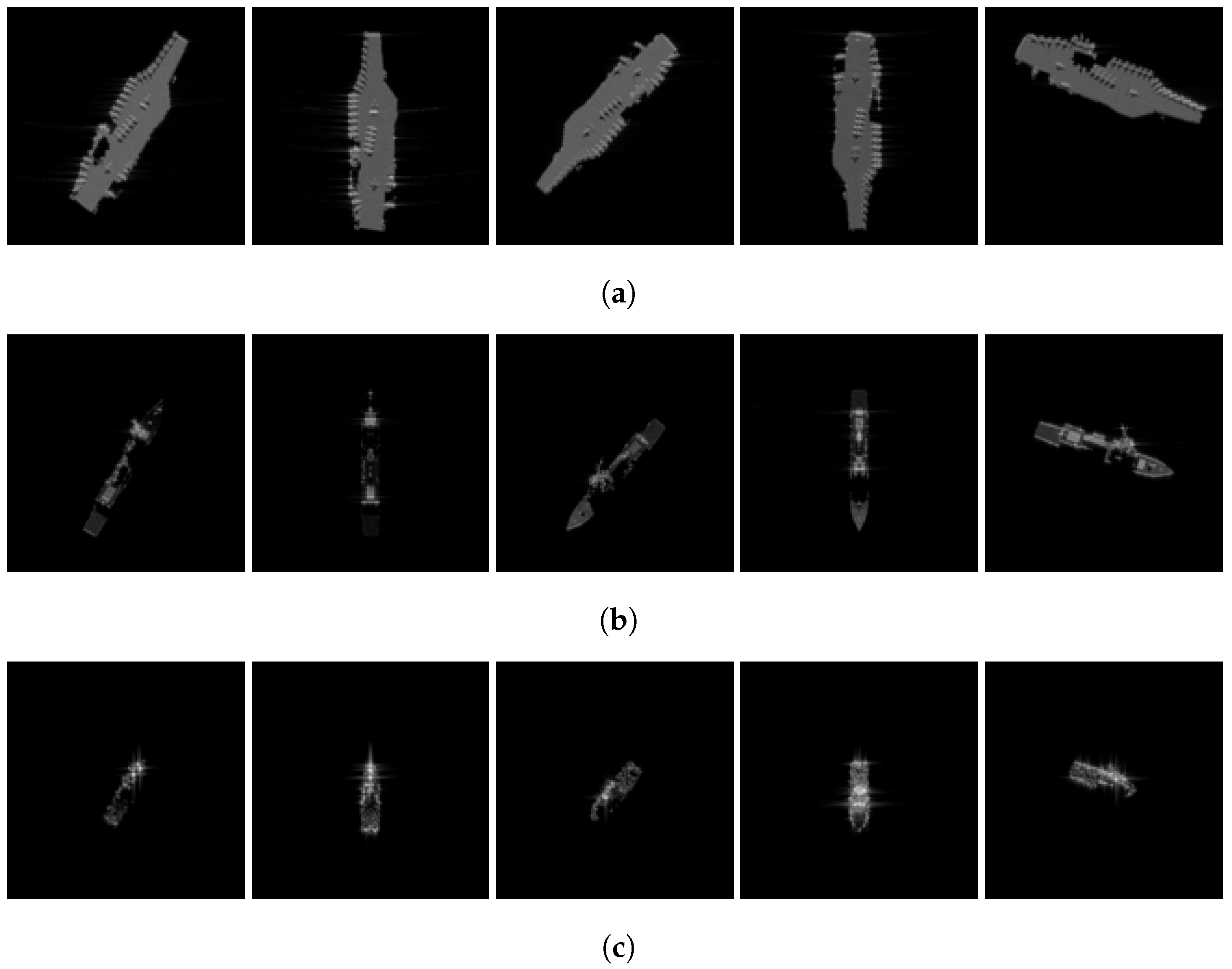
To validate the effectiveness of the proposed method for SAR image generation at unknown azimuths under small-sample conditions, experiments are conducted using a self-constructed dataset that integrates both simulated and measured data. The simulated dataset is generated using RaySAR software and comprises three categories of ship targets: large, medium, and small. Each category covers a full range of azimuth angles from 0° to 360°. These multi-angle SAR image samples are obtained through rigorous target geometric modeling, EM scattering computation, and SAR imaging simulation. Part of the simulated dataset is shown in the Figure 3. This dataset offers several advantages, including controllable imaging parameters, precise azimuth labels, and well-defined target-scattering structures, making it suitable for evaluating the model’s generative performance under ideal conditions.

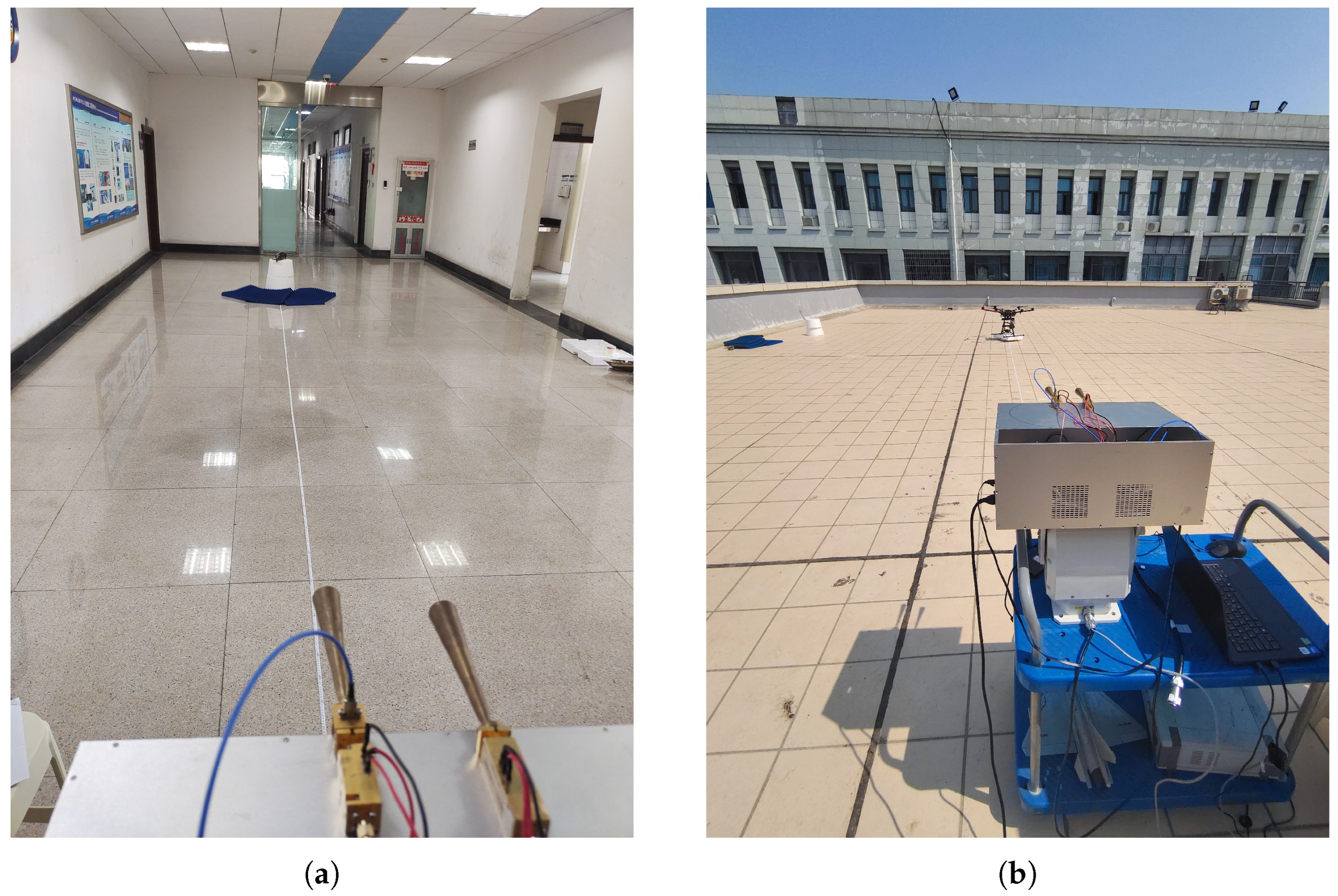
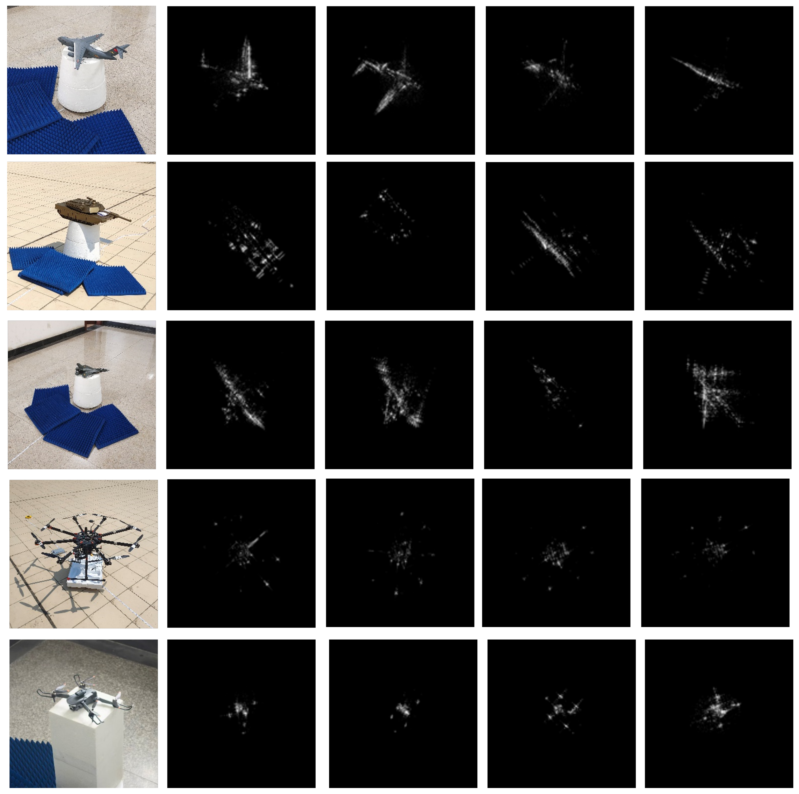
The measured dataset was acquired using a millimeter-wave (mmWave) radar system with a center frequency of $213.84$ GHz and a bandwidth of $28.8$ GHz. This frequency was selected according to the scaled model measurement setting used in this work. Since the measured targets are scaled models, a higher operating frequency is required to preserve the electrical size of the target and to maintain electromagnetic similarity with the corresponding full-scale scenario. Specifically, if the target geometry is reduced by a scale factor, the radar frequency should be increased by approximately the same factor to keep the ratio between the target size and wavelength unchanged. Therefore, the 213.84 GHz radar system enables the scaled targets to produce physically meaningful high-resolution scattering responses. It encompasses SAR images of diverse targets across multiple scales, including tanks, aircraft, and small-to-medium-sized UAVs. Each target category provides full 0°–360° azimuth coverage. Given the rich variety of target types and their distinct structural characteristics, this dataset effectively captures the complex electromagnetic scattering mechanisms and dynamic background features inherent in real-world SAR imaging scenarios. The measured experimental scenarios and measured data are shown in Figure 4 and Figure 5, respectively.

4.2. Experiment Result

4.2.1. Experiment Setup

To simulate the practical scenario of limited observation angles in SAR image acquisition, sparse angular sampling is performed on the original multi-aspect dataset using azimuth intervals of 5° and 10°. Specifically, when the sampling interval is set to 5°, a total of 72 known observation angles are used for training, while a 10° interval provides 36 known observation angles for training. Under these two sparse sampling settings, the intermediate azimuth angles between adjacent known views are excluded from the training set and used as testing angles. Based on these two sparse sampling settings, the unseen intermediate angle images located between adjacent known azimuth angles are selected as the generation targets, so as to evaluate the interpolation capability of the proposed model for unknown angle SAR image generation under different levels of angular sparsity. All SAR images are resized to $128\times 128$. The scattering center extraction is performed on complex-valued SAR images to preserve both amplitude and phase information. After the scattering center prior is obtained, the SAR images are converted to amplitude images and normalized before being used as inputs for training and generation in the diffusion model.

In the implementation of the PSF-constrained ISTA module, the PSF was constructed according to the radar center frequency, signal bandwidth, angular aperture, and image-plane sampling interval. Specifically, the center frequency and bandwidth of the measured dataset were calculated using $f_0=213.84$ GHz and $B=28.8$ GHz. The angular aperture was set to $\mathsf{\Delta }\varphi =6°$. The PSF kernel size was $129\times 129$, and the spatial sampling intervals along the range and azimuth directions were both set to $0.1 \mathrm{m}$. For the ISTA solver, the sparsity regularization coefficient was set to $\lambda =0.3$, the maximum number of iterations was set to 300, and the convergence tolerance was set to ${10}^{-4}$.

For comparative experiments, a conditional GAN (cGAN) constructed based on the same scattering center-guided framework is selected as the baseline method and compared with the proposed scattering map prior-guided diffusion model, in order to investigate the performance differences between different generative paradigms in unknown angle SAR image-generation tasks. Both methods take the target category, azimuth information, and the dominant scattering maps extracted by PSF-constrained ISTA as conditional inputs. In addition, a linear image-domain interpolation method is introduced as a non-learning baseline. Specifically, for a target unseen azimuth, the SAR images from its two neighboring known azimuths are linearly fused according to their angular distances. This baseline is used to evaluate whether the proposed method can generate unseen-azimuth SAR images beyond simple neighboring-view interpolation.

To comprehensively evaluate the generation quality, both qualitative and quantitative analyses are conducted. Qualitative evaluation is mainly performed through visual comparison of the preservation of dominant scattering structures, bright scattering responses, and overall target contours. Quantitative evaluation adopts PSNR, SSIM, LPIPS, and FID to assess pixel-wise consistency, structural similarity, perceptual discrepancy, and distribution-level consistency between the generated images and the ground-truth images.

All experiments in this paper were conducted under the Windows 10 operating system. The experimental platform was equipped with an NVIDIA RTX 3090 GPU, an Intel Core i7-10700KF CPU, and 64 GB of RAM. Model training and testing were implemented based on the PyTorch 2.0.1 deep learning framework, and the AdamW optimizer was adopted for parameter updating, with the learning rate set to $1\times {10}^{-4}$.

4.2.2. PSF-Constrained ISTA Extraction Results

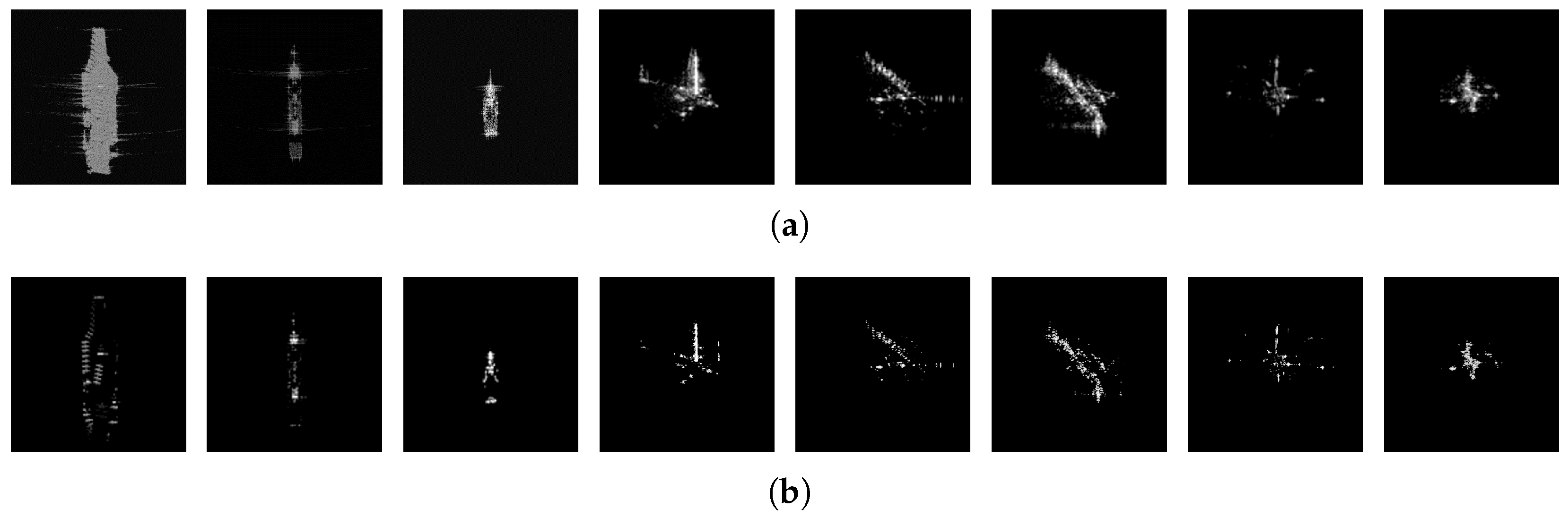
Figure 6 presents the dominant scattering center extraction results obtained by the PSF-constrained ISTA method on both simulated and measured datasets. It can be observed that the original SAR images usually contain target scattering responses, background clutter, and sidelobe spreading introduced by the imaging system. After sparse reconstruction using PSF-constrained ISTA, the positions of strong scattering responses are effectively highlighted, while weak scattering components and background clutter are significantly suppressed. From the simulated data, it can be observed that for structurally complex targets such as aircraft carriers and destroyers, the prominent scattering regions corresponding to distinctive structures—such as the carrier-based aircraft on the aircraft carrier, the island structure located in the lower-right region of the image, and the bridge structure in the upper middle part of the destroyer—are well preserved in the extracted scattering maps.

Further observation of the measured data shows that for relatively small targets with simpler scattering structures, such as tank models and small unmanned aerial vehicles (UAVs), the dominant bright scattering responses can also be clearly represented in the sparse scattering maps. These results demonstrate that the proposed PSF-constrained ISTA scattering center extraction method not only effectively suppresses weak scattering structures and background interference in the original SAR images, but also accurately extracts the dominant scattering structures closely related to the target electromagnetic scattering mechanism. This provides a physically meaningful intermediate representation for subsequent unknown angle SAR image generation.

4.2.3. Analysis of Generation Results on the Simulated Dataset

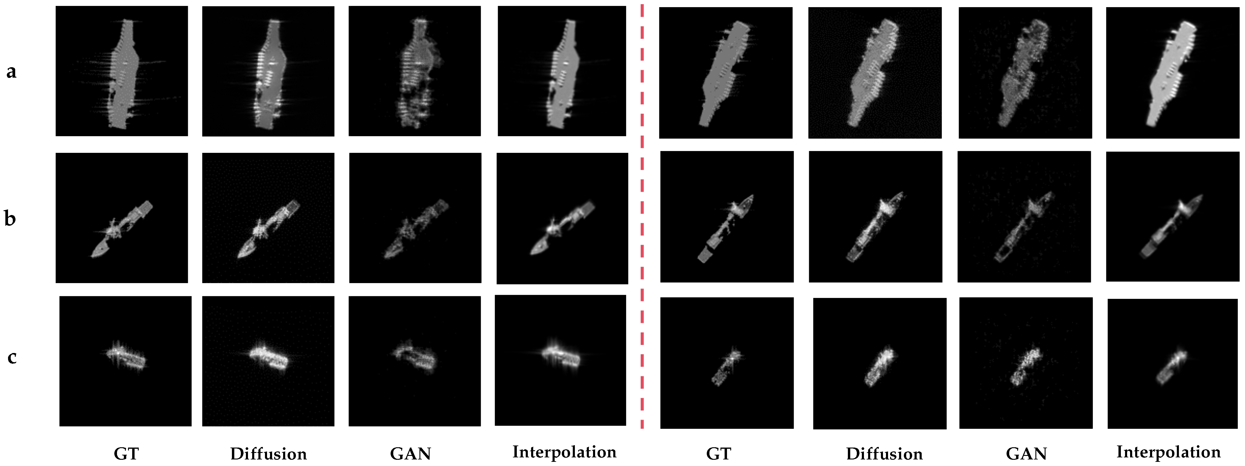
Figure 7 present the experimental results of unknown-azimuth SAR image generation on the simulated dataset under different angular sampling intervals of 5° and 10°. The proposed scattering center prior-guided diffusion model is compared with the baseline GAN method and the image-domain interpolation method. Three representative ship targets with different sizes are selected for comparative analysis.

By comparing the generated results of different target categories, it can be seen that scattering centers mainly characterize the spatial locations and response distributions of the dominant electromagnetic scattering structures of the target. Therefore, the prior formed by fusing scattering centers from known observation angles within a small angular range can provide relatively stable structural skeleton information for image generation at unknown azimuth angles. This enables the model to rely not only on statistical features in the image domain, but also on explicit guidance from the dominant scattering structures of the target. Moreover, from the perspective of physical imaging mechanisms, such a prior can further enhance the model’s ability to infer scattering patterns at unknown viewing angles. As a result, the diffusion model can maintain the continuity of the target’s dominant scattering distribution along its longitudinal direction. For targets with distinct local structures, the proposed method can also realistically recover the corresponding local strong scattering highlights.

A further comparison among the three methods shows that the proposed diffusion model has clear advantages in preserving dominant scattering structures and target contours. Specifically, the diffusion-generated images present sharper scattering responses, more accurate strong scatterer points, and fewer irrelevant background artifacts. The GAN-based method can generate the overall target appearance, but its results often contain local structural blurring, unstable scattering responses, and incomplete target contours under sparse angular sampling. The interpolation method can retain the coarse target shape because it directly uses neighboring known-view SAR images. However, compared with the reference images and the diffusion results, the interpolated images exhibit less realistic brightness distribution and excessively high local contrast. Some scattering regions are over-enhanced, while the intensity transition between strong scatterers and the background becomes unnatural.

To further objectively evaluate the quality of the generated results on the simulated dataset, several quantitative metrics, including SSIM, PSNR, FID, and LPIPS, are used to assess the performance of the two generation methods. The evaluation results are reported in

Table 1. Quantitative comparison on simulated SAR images under different sampling intervals. The best results are highlighted in bold. ↑ indicates that a higher value is better, while ↓ indicates that a lower value is better.

Sampling Interval	Method	Target	SSIM ↑	PSNR ↑	FID ↓	LPIPS ↓
5°	Diffusion	Aircraft carrier model	0.8653	21.6535	199.0848	0.0959
		Destroyer model	0.9459	28.0756	70.2586	0.0525
		Fishing vessel model	0.9605	26.2034	121.6923	0.0800
	GAN	Aircraft carrier model	0.8291	23.5225	351.0320	0.1397
		Destroyer model	0.9343	29.5803	157.2875	0.0594
		Fishing vessel model	0.9452	26.3564	191.0166	0.0760
	Interpolation	Aircraft carrier model	0.8335	18.1100	84.0603	0.1233
		Destroyer model	0.9386	26.8540	44.4199	0.0874
		Fishing vessel model	0.9479	32.4672	50.6886	0.0857
10°	Diffusion	Aircraft carrier model	0.8176	22.4864	215.2628	0.1260
		Destroyer model	0.9094	24.0847	127.4658	0.1066
		Fishing vessel model	0.9488	26.7417	151.5941	0.0999
	GAN	Aircraft carrier model	0.7501	22.3557	324.2745	0.2073
		Destroyer model	0.8305	24.6572	159.8239	0.1732
		Fishing vessel model	0.8751	30.5345	282.6289	0.1764
	Interpolation	Aircraft carrier model	0.8083	17.6277	84.8863	0.1526
		Destroyer model	0.9018	21.2273	43.1309	0.1123
		Fishing vessel model	0.9418	26.2220	64.2374	0.1058

. Among these metrics, SSIM and PSNR reflect the structural and pixel-level similarity between the generated images and the real images, FID measures the distribution discrepancy between generated samples and real samples, and LPIPS characterizes the perceptual distance in the deep feature space.

According to the table. Under both 5° and 10° sampling intervals, the proposed diffusion model generally achieves higher SSIM and lower LPIPS than the GAN baseline, indicating better structural preservation and perceptual similarity. The GAN baseline obtains higher PSNR values in some cases, while the interpolation baseline achieves lower FID values in several cases. Therefore, the quantitative results show that different metrics emphasize different aspects of generation quality. Overall, the proposed diffusion model shows more stable performance in preserving dominant scattering structures and target contours, while the detailed reasons for the metric differences are further discussed in Section 5.

4.2.4. Analysis of Generation Results on the Measured Dataset

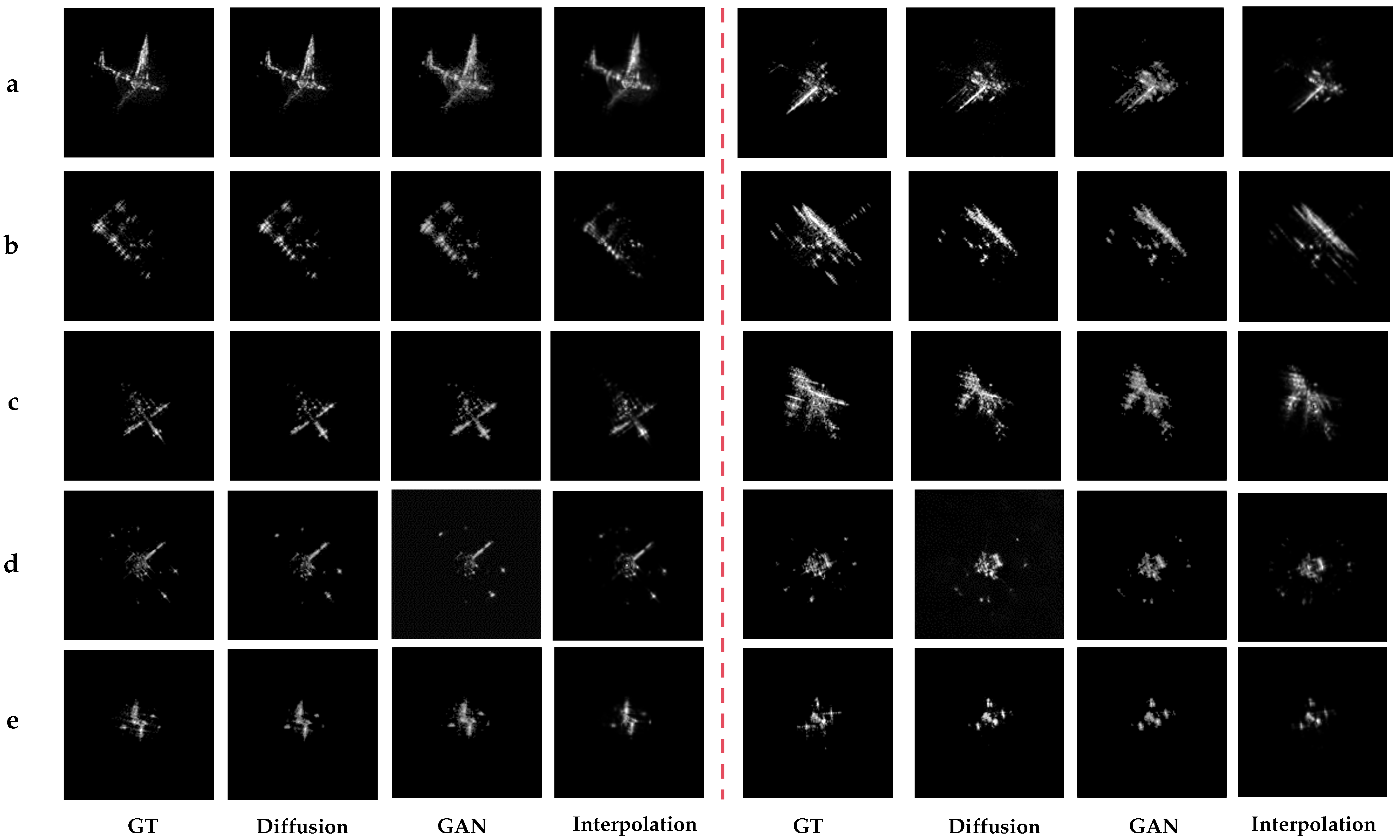
Figure 8 shows the generation results on the measured dataset. From the 5° sampling results, it can be observed that under relatively dense azimuth sampling conditions, the unknown intermediate angle maintains strong continuity with its adjacent known views. As a result, the overall generation difficulty is relatively low, and all compared methods are able to recover, to a certain extent, the dominant scattering points and main target structure.

A further comparison shows that the diffusion model performs better in reconstructing strong scattering regions at unknown angles. Specifically, the strong scattering highlights generated by the diffusion model are more prominent, and the spatial distribution of the strong scattering regions is more consistent with that of the real images. This advantage is particularly evident in typical strong scattering regions, such as the fuselage-wing junctions of aircraft models, the edges of the main body of tanks, and the locally protruding wing structures of UAVs.

When the sampling interval increases to 10°, the difference between the unknown angles and the known angles becomes more pronounced, and the discrepancy among the fused scattering centers also increases. Under such sparser observation conditions, the model must infer the evolution of the target scattering structure with azimuth variation, making the generation task significantly more challenging. As shown by the results on the right side of the figure, the generation quality of both methods degrades to some extent compared with the 5° sampling condition. This degradation is mainly reflected in reduced contour clarity, weakened local strong scattering structures, and increased background artifacts. In contrast, the SAR images generated by the diffusion model are still able to preserve the main scattering skeleton of the target more clearly, with relatively more prominent strong scattering regions and local structural layouts that are closer to those in the real images.

The quantitative evaluation results on the measured dataset are listed in

Table 2. Quantitative comparison of different methods on measured SAR images under different sampling intervals. The best results are highlighted in bold. ↑ indicates that a higher value is better, while ↓ indicates that a lower value is better.

Sampling Interval	Method	Target	SSIM ↑	PSNR ↑	FID ↓	LPIPS ↓
5°	Diffusion	Large aircraft model	0.9816	39.5005	17.0284	0.0163
		Tank model	0.9668	36.0172	35.6660	0.0439
		Small aircraft model	0.9722	35.6582	22.0490	0.0342
		Large UAV	0.9861	41.9316	35.3487	0.0213
		Small UAV	0.9865	39.6067	19.4723	0.0171
	GAN	Large aircraft model	0.9626	36.7128	37.5177	0.0285
		Tank model	0.9511	35.1767	62.1365	0.0530
		Small aircraft model	0.9697	34.9894	38.7741	0.0383
		Large UAV	0.9814	39.4487	83.0382	0.0323
		Small UAV	0.9851	39.1279	32.0971	0.0174
	Interpolation	Large aircraft model	0.9622	32.0231	35.8688	0.0861
		Tank model	0.9504	32.4866	45.8223	0.0691
		Small aircraft model	0.9648	31.0389	36.6875	0.0725
		Large UAV	0.9650	32.0972	50.8944	0.0862
		Small UAV	0.9810	36.1091	22.6951	0.0421
10°	Diffusion	Large aircraft model	0.9251	28.2932	44.2522	0.0849
		Tank model	0.9234	29.3013	68.5044	0.0896
		Small aircraft model	0.9403	28.8647	43.2131	0.0789
		Large UAV	0.9503	33.6262	60.9765	0.0716
		Small UAV	0.9738	33.3900	38.1664	0.0401
	GAN	Large aircraft model	0.9423	34.0811	51.3912	0.0859
		Tank model	0.9049	30.4350	73.1851	0.0917
		Small aircraft model	0.9318	28.5969	37.8454	0.0802
		Large UAV	0.9520	34.6493	54.3441	0.0781
		Small UAV	0.9704	34.6275	38.9997	0.0403
	Interpolation	Large aircraft model	0.9415	29.6122	45.8566	0.0659
		Tank model	0.9244	29.8859	51.3819	0.0912
		Small aircraft model	0.9320	29.0543	46.7268	0.0814
		Large UAV	0.9446	30.3187	62.8565	0.0766
		Small UAV	0.9592	32.7211	36.6406	0.0470

. Under the 5° sampling condition, the proposed diffusion model achieves better average performance than the GAN and interpolation baselines in most metrics. These results indicate that, for this task, the scattering center-guided diffusion model not only recovers unknown-azimuth SAR images more accurately at the pixel and structural levels, but also produces results that are closer to real SAR images in terms of perceptual quality and distribution consistency. When the angular sampling interval increases from 5° to 10°, the discrepancy between the unknown intermediate angles and the adjacent known angles becomes significantly larger, causing the generation task to shift from relatively straightforward neighboring view interpolation to the more challenging problem of sparse view generation.

5. Discussion

The experimental results indicate that under both 5° and 10° sampling intervals, the proposed diffusion model achieves better performance than the GAN baseline in terms of SSIM, FID, and LPIPS, while GAN obtains higher PSNR values in some cases. This phenomenon can be partly attributed to the smoother and more averaged responses generated by GAN, which reduce pixel-wise intensity errors and thus improve PSNR. In contrast, the proposed diffusion model, guided by scattering-center priors, tends to preserve sharper and more distinct scattering responses. Since simulated SAR images are dominated by sparse high-intensity scattering centers, slight spatial shifts or local intensity deviations of these scatterers may lead to larger pixel-wise errors, thereby reducing the PSNR value. It is also observed that the image-domain interpolation baseline achieves lower FID values than both learning-based methods in several cases. This result is reasonable because the interpolation method directly uses neighboring real SAR images to synthesize the target unknown azimuth image. As a result, the interpolated images naturally inherit the global intensity statistics, background distribution of the real SAR data, making their feature distribution closer to that of the reference set and thus leading to lower FID values.

When the sampling interval increases from 5° to 10°, the GAN method, the interpolation method, and the proposed diffusion method all exhibit performance degradation. This degradation is mainly caused by the reduced correlation between neighboring aspect views. Under the 5° setting, adjacent SAR images still share relatively continuous dominant scattering structures, and the fused scattering center prior can provide reliable structural guidance for the target unknown azimuth. However, under the 10° setting, the angular distance between known and unknown azimuths becomes larger, and the aspect-dependent scattering variation becomes more significant; some dominant scattering centers may shift, disappear, or newly emerge. Consequently, the fused scattering-center prior becomes less accurate, and the uncertainty of the generation process increases. For the interpolation method, this larger angular gap also makes direct image-domain interpolation less reliable, since it cannot effectively model nonlinear scattering variations and may produce unrealistic brightness distribution, excessive local contrast, or blurred scattering details.

It should also be acknowledged that the current component-wise ablation analysis remains limited. The present experiments mainly evaluate the overall effectiveness of the proposed scattering center prior-guided diffusion framework by comparing it with the scattering-guided GAN and image-domain interpolation baselines. However, the individual contributions of the PSF-constrained ISTA extraction module, the scattering prior fusion strategy, and the category and azimuth conditions have not yet been systematically quantified. In particular, completely removing the scattering center prior would change the conditional formulation and network input structure of the current framework, making a strictly controlled comparison less straightforward. Future work will therefore conduct more comprehensive component-wise experiments, including alternative scattering center extraction methods, and different prior fusion strategies to further clarify the contribution of each component.

The influence of the scattering center prior is also related to target structural complexity. For targets with relatively simple and stable scattering structures, the dominant scatters usually vary smoothly with azimuth, so the fused prior remains effective even under moderately sparse angular sampling. In contrast, complex targets, such as aircraft with wings, tails, or ships with multiple corner-like scattering components, with different parts may dominate the SAR response at different azimuths. These targets usually contain multiple discrete and aspect-sensitive scattering regions. Different components may dominate the SAR scattering response at different observation azimuths. When the angular interval is small, adjacent views still preserve partially similar scattering structures, and the fused scattering center prior can provide relatively reliable structural guidance. However, when the sampling interval increases, the visibility and intensity of these components may change significantly.

Overall, the extracted scattering centers still provide useful structural cues for the main target geometry and dominant scattering regions. Compared with purely image-domain generative methods, the proposed method can still benefit from these physically interpretable priors to maintain the overall target structure and enhance the consistency of strong scattering regions. The performance degradation under the 10° setting mainly indicates that the linear fusion strategy becomes less accurate when the aspect-dependent scattering variation is more significant. This observation suggests that future work can further improve the current framework by introducing nonlinear, adaptive, or geometry aware scattering prior fusion strategies.

6. Conclusions

This paper addresses the problem of unknown-azimuth SAR image generation under small-sample conditions and proposes a conditional diffusion generation method guided by scattering center physical priors. Compared with conventional generative methods that learn distribution mappings only in the image domain, the proposed method starts from the SAR imaging mechanism. Specifically, dominant scattering centers are first extracted from known azimuth SAR images using PSF-constrained ISTA, yielding sparse and physically interpretable scattering center representations. Then, the target category, observation angle, and dominant scattering map are jointly used as conditional inputs to train the diffusion model to learn the relationship between conditional representations and SAR images. Finally, scattering maps from known azimuth angles are fused to construct an approximate scattering prior for the unknown azimuth, thereby enabling SAR image generation at unknown angles. By explicitly introducing constraints from dominant scattering structures into the generation process, the proposed method enables the deep generative model to simultaneously exploit image distribution learning and maintain consistency with SAR scattering mechanisms.

In terms of experimental validation, a simulated dataset containing ship targets of different sizes and categories is constructed based on RaySAR. In addition, a measured dataset containing multiple target categories, including aircraft, tanks, and UAVs, is established using a millimeter wave radar system. Unknown angle interpolation generation experiments are systematically conducted under two sparse sampling settings, namely 5° and 10° azimuth intervals. The experimental results demonstrate that, compared with the GAN method based on the same scattering map guided framework and interpolation method, the proposed method can better recover the dominant scattering structures of targets at unknown azimuth angles on both simulated and measured datasets, showing superior generation quality in terms of structural clarity, contour integrity, and dominant scattering center representation.

Although the proposed method preliminarily verifies the feasibility of unknown-azimuth SAR image generation under small-sample conditions, several issues remain to be further investigated. First, the current experiments mainly focus on unknown angle interpolation generation under 5° and 10° sparse sampling settings. Although these settings can effectively reflect the performance of the method in small-sample scenarios, its generation capability under larger angular spans, more sparsely observed conditions, and continuously missing angular sectors still requires further study. Second, the scattering center prior constructed in this paper is mainly obtained by fusing scattering maps from known azimuth angles, which is essentially an approximate physical structural constraint. In future work, we will further investigate the continuous and discontinuous evolution of dominant scattering centers with respect to observation angles, and explore nonlinear, adaptive, and geometry-aware scattering-prior fusion strategies. Overall, achieving stronger physical constraints and better angular generalization remains an important direction for future research.

References

- Moreira, A.; Prats-Iraola, P.; Younis, M.; Krieger, G.; Hajnsek, I.; Papathanassiou, K.P. A tutorial on synthetic aperture radar. IEEE Geosci. Remote Sens. Mag. 2013, 1, 6–43. [Google Scholar] [CrossRef]
- Curlander, J.C.; McDonough, R.N. Synthetic Aperture Radar; Wiley: New York, NY, USA, 1991; Volume 11. [Google Scholar]
- Passah, A.; Sur, S.N.; Abraham, A.; Kandar, D. Synthetic Aperture Radar image analysis based on deep learning: A review of a decade of research. Eng. Appl. Artif. Intell. 2023, 123, 106305. [Google Scholar] [CrossRef]
- Peter, E.; Ang, L.M.; Seng, K.P.; Srivastava, S. Recent Advances in Deep Learning for SAR Images: Overview of Methods, Challenges, and Future Directions. Sensors 2026, 26, 1143. [Google Scholar] [CrossRef] [PubMed]
- Huang, Z.; Zhang, X.; Tang, Z.; Xu, F.; Datcu, M.; Han, J. Generative artificial intelligence meets synthetic aperture radar: A survey. IEEE Geosci. Remote Sens. Mag. 2024, 14, 6–48. [Google Scholar] [CrossRef]
- Li, X.; Liu, L.; Wan, G.; Zheng, F.; Guo, S.; Sun, G.; Wang, Z.; Liu, X. Physics-Driven SAR Target Detection: A Review and Perspective. Remote Sens. 2026, 18, 200. [Google Scholar] [CrossRef]
- Chen, H.; Zhang, Y.; Wang, H.; Ding, C. SAR imaging simulation for urban structures based on analytical models. IEEE Geosci. Remote Sens. Lett. 2012, 9, 1127–1131. [Google Scholar] [CrossRef]
- Chen, Z.; Zeng, Z.; Huang, Y.; Wan, J.; Tan, X. SAR raw data simulation for fluctuant terrain: A new shadow judgment method and simulation result evaluation framework. IEEE Trans. Geosci. Remote Sens. 2021, 60, 5215018. [Google Scholar] [CrossRef]
- Ding, B.; Wen, G. Exploiting multi-view SAR images for robust target recognition. Remote Sens. 2017, 9, 1150. [Google Scholar] [CrossRef]
- Zhang, H.; Wei, S.; Cheng, Y.; Li, S.; Min, R.; Li, J.; Wang, M.; Cui, G. Efficient FMCW Radar Interference Suppression via Adaptive Learning Framework with Localized Sparse Prior. IEEE Trans. Microw. Theory Tech. 2026, 74, 3149–3162. [Google Scholar] [CrossRef]
- Yang, X.; Yang, W.; Song, H.; Huang, P. Polarimetric SAR image classification using geodesic distances and composite kernels. IEEE J. Sel. Top. Appl. Earth Obs. Remote Sens. 2018, 11, 1606–1614. [Google Scholar] [CrossRef]
- Cui, Y.; Liu, Z.; Ruan, L.; Sheng, B.; Wang, N.; Xiao, X.; Bian, X. An Azimuth-Continuously Controllable SAR Image Generation Algorithm Based on GAN. Remote Sens. 2025, 17, 3763. [Google Scholar] [CrossRef]
- Goodfellow, I.J.; Pouget-Abadie, J.; Mirza, M.; Xu, B.; Warde-Farley, D.; Ozair, S.; Courville, A.; Bengio, Y. Generative adversarial nets. Adv. Neural Inf. Process. Syst. 2014, 27, 2672–2680. [Google Scholar]
- Mirza, M.; Osindero, S. Conditional generative adversarial nets. arXiv 2014, arXiv:1411.1784. [Google Scholar]
- Ho, J.; Jain, A.; Abbeel, P. Denoising diffusion probabilistic models. Adv. Neural Inf. Process. Syst. 2020, 33, 6840–6851. [Google Scholar]
- Nichol, A.Q.; Dhariwal, P. Improved denoising diffusion probabilistic models. In Proceedings of the International Conference on Machine Learning; PMLR: New York, NY, USA, 2021; pp. 8162–8171. [Google Scholar]
- Dhariwal, P.; Nichol, A. Diffusion models beat gans on image synthesis. Adv. Neural Inf. Process. Syst. 2021, 34, 8780–8794. [Google Scholar]
- Daubechies, I.; Defrise, M.; De Mol, C. An iterative thresholding algorithm for linear inverse problems with a sparsity constraint. Commun. Pure Appl. Math. 2004, 57, 1413–1457. [Google Scholar] [CrossRef]
- Liu, H.; Jiu, B.; Li, F.; Wang, Y. Attributed scattering center extraction algorithm based on sparse representation with dictionary refinement. IEEE Trans. Antennas Propag. 2017, 65, 2604–2614. [Google Scholar] [CrossRef]
- Çetin, M.; Karl, W.C. Feature-enhanced synthetic aperture radar image formation based on nonquadratic regularization. IEEE Trans. Image Process. 2001, 10, 623–631. [Google Scholar] [CrossRef] [PubMed]
- Holtzman, J.C.; Stiles, J.A.; Frost, V.S.; Kaupp, V.H.; Komp, E.E. A digital computation technique for radar scene simulation: NEWSLAR. Simulation 1979, 32, 183–192. [Google Scholar] [CrossRef]
- Franceschetti, G.; Migliaccio, M.; Riccio, D.; Schirinzi, G. SARAS: A synthetic aperture radar (SAR) raw signal simulator. IEEE Trans. Geosci. Remote Sens. 2002, 30, 110–123. [Google Scholar]
- Potter, L.C.; Moses, R.L. Attributed scattering centers for SAR ATR. IEEE Trans. Image Process. 1997, 6, 79–91. [Google Scholar] [CrossRef] [PubMed]
- Gerry, M.J.; Potter, L.C.; Gupta, I.J.; Van Der Merwe, A. A parametric model for synthetic aperture radar measurements. IEEE Trans. Antennas Propag. 2002, 47, 1179–1188. [Google Scholar]
- Akyildiz, Y.; Moses, R.L. Scattering center model for SAR imagery. In Proceedings of the SAR Image Analysis, Modeling, and Techniques II; SPIE: Bellingham, DC, USA, 1999; Volume 3869, pp. 76–85. [Google Scholar]
- Cimmino, S.; Franceschetti, G.; Iodice, A.; Riccio, D.; Ruello, G. Efficient spotlight SAR raw signal simulation of extended scenes. IEEE Trans. Geosci. Remote Sens. 2003, 41, 2329–2337. [Google Scholar] [CrossRef]
- Ling, H.; Chou, R.C.; Lee, S.W. Shooting and bouncing rays: Calculating the RCS of an arbitrarily shaped cavity. IEEE Trans. Antennas Propag. 1989, 37, 194–205. [Google Scholar] [CrossRef]
- Chang, Y.L.; Chiang, C.Y.; Chen, K. SAR image simulation with application to target recognition. Prog. Electromagn. Res. 2011, 119, 35–57. [Google Scholar] [CrossRef]
- Kunz, K.S.; Luebbers, R.J. The Finite Difference Time Domain Method for Electromagnetics; CRC Press: Boca Raton, FL, USA, 1993. [Google Scholar]
- Harrington, R.F. Field Computation by Moment Methods; Wiley-IEEE Press: Piscataway, NJ, USA, 1993. [Google Scholar]
- Auer, S.; Hinz, S.; Bamler, R. Ray-tracing simulation techniques for understanding high-resolution SAR images. IEEE Trans. Geosci. Remote Sens. 2009, 48, 1445–1456. [Google Scholar]
- Balz, T.; Stilla, U. Hybrid GPU-based single-and double-bounce SAR simulation. IEEE Trans. Geosci. Remote Sens. 2009, 47, 3519–3529. [Google Scholar] [CrossRef]
- Aguilar, A.G.; van Tonder, J.; Jakobus, U.; Illenseer, F. Overview of recent advances in the electromagnetic field solver FEKO. In Proceedings of the 2015 9th European Conference on Antennas and Propagation (EuCAP); IEEE: New York, NY, USA, 2015; pp. 1–5. [Google Scholar]
- Zhang, J.; Liu, Z.; Jiang, W.; Liu, Y.; Zhou, X.; Li, X. Application of deep generative networks for SAR/ISAR: A review. Artif. Intell. Rev. 2023, 56, 11905–11983. [Google Scholar] [CrossRef]
- Cui, Z.; Zhang, M.; Cao, Z.; Cao, C. Image Data Augmentation for SAR Sensor via Generative Adversarial Nets. IEEE Access 2019, 7, 42255–42268. [Google Scholar] [CrossRef]
- Feng, G. Research on SAR Image Simulation Based on Deep Generative Learning. Master’s Thesis, University of Electronic Science and Technology of China, Chengdu, China, 2021. (In Chinese) [Google Scholar]
- Liu, Z.; Niu, S.; Qiu, X.; Peng, L.; Shang, Y.; Zhong, L.; Ding, C. A differentiable method for novel view SAR image generation via 3D Gaussian Splatting. ISPRS J. Photogramm. Remote Sens. 2026, 231, 167–195. [Google Scholar] [CrossRef]
- Gao, H.; Huang, T.; Guo, L.; He, J.; Eldar, Y.C. Diffusion-Prior Split Gibbs Sampling for Synthetic Aperture Radar Imaging under Incomplete Measurements. arXiv 2025, arXiv:2512.02768. [Google Scholar]
- Lei, Z.; Xu, F.; Wei, J.; Cai, F.; Wang, F.; Jin, Y.Q. SAR-NeRF: Neural radiance fields for synthetic aperture radar multiview representation. IEEE Trans. Geosci. Remote Sens. 2024, 62, 5221415. [Google Scholar] [CrossRef]
- Zhang, X.; Zhuang, Y.; Guo, Q.; Yang, H.; Qian, X.; Cheng, G.; Han, J.; Huang, Z. Φ-GAN: Physics-inspired GAN for generating SAR images under limited data. In Proceedings of the IEEE/CVF International Conference on Computer Vision; IEEE: New York, NY, USA, 2025; pp. 29075–29085. [Google Scholar]
- Zhang, F.; Wu, X.; Ma, F.; Yin, Q.; Hu, Y. GeoDiff-SAR: A Geometric Prior Guided Diffusion Model for SAR Image Generation. arXiv 2026, arXiv:2601.03499. [Google Scholar]
Figure 1.
Overall processing flowchart of the proposed PSF-constrained scattering center prior-guided conditional diffusion method for unknown-azimuth SAR image generation.
Figure 2.
Flowchart of PSF-constrained scattering center extraction via ISTA.
Figure 3.
Examples of different ship samples in the simulated dataset: (a) aircraft carrier model; (b) destroyer model; (c) fishing vessel model.
Figure 4.
Illustration of the measured experimental scenarios. (a) Indoor scenario. (b) Outdoor scenario.
Figure 5.
Examples of different target samples in the measured dataset. Rows 1–5 correspond to a large aircraft model, a tank model, a small aircraft model, a large UAV, and a small UAV, respectively.
Figure 6.
Scattering center extraction results obtained by PSF-constrained ISTA: (a) original SAR images; (b) corresponding extracted scattering center maps.
Figure 7.
Generation results on the simulated dataset under different angular sampling intervals. The regions to the left and right of the red line correspond to the 5° and 10° sampling intervals, respectively. (a–c) represent the aircraft carrier model, destroyer model, and fishing boat model, respectively.
Figure 8.
Generation results on the measured dataset under different angular sampling intervals. (a–e) represent the large aircraft model, tank model, small aircraft model, large UAV, and small UAV, respectively. The regions to the left and right of the red line correspond to the 5° and 10° sampling intervals, respectively.