Glacier Boundary Extraction over the Tibetan Plateau Using a Double Random Forest Model with Multi-Temporal Sentinel-1/2 Data

Highlights

What are the main findings?

• A feature-fusion-driven Double-RF framework significantly improves the identification accuracy of complex glacier types, particularly debris-covered and glaciers in shadow on the Tibetan Plateau.
• Multi-temporal feature integration captures seasonal dynamics and reduces environmental noise, leading to more robust and stable classification results across diverse Tibetan Plateau basins.
• Tibetan Plateau glaciers exhibit strong spatial heterogeneity with distinct topographic patterns; clean glaciers dominating mid-to-high elevations (5000–6500 m) and debris-covered glaciers concentrated at lower elevations (4500–5000 m).

What are the implications of the main findings?

• The proposed approach advances automated glacier identification toward large-scale, high-precision applications in complex mountainous regions.
• The results provide a reliable basis for glacier evolution studies and contribute to improved assessments of water resources and cryospheric hazards under climate change across the Tibetan Plateau.

Abstract

Glacier boundary extraction on the Tibetan Plateau (TP) faces persistent challenges due to rugged terrain, seasonal snow, extensive debris cover, and topographic shadows. Traditional methods utilizing single-source or single-temporal data often yield limited accuracy. Thus, we propose an automated Double Random Forest (Double-RF) framework integrating single- and multi-temporal features from Sentinel-1 (SAR) and Sentinel-2 (Optical) data within the Google Earth Engine. We established a multidimensional feature space comprising spectral, textural, polarimetric, and topographic attributes. Feature optimization was performed using importance metrics and out-of-bag (OOB) error. A hierarchical classification strategy was employed: the first RF identifies clean glaciers and glaciers in shadow, while the second RF executes refined boundary extraction of debris-covered glaciers to mitigate spectral confusion. The results indicate that the Double-RF method significantly achieves an overall accuracy exceeding 0.84 across all sub-basins and reaching above 0.95 at best. The derived glacier inventory reveals a distinct spatial pattern: higher concentrations in the western and peripheral regions compared to the eastern and interior TP. Glaciers are predominantly distributed on shaded aspects with gentle-to-moderate slopes, highlighting the combined influence of climatic gradients and topographic controls. This multi-source, multi-temporal fusion strategy provides a robust methodological foundation for long-term glacier monitoring over the TP.

1. Introduction

In recent decades, global climate change has emerged as a central concern across nations and scientific disciplines. Glaciers, often referred to as the “cooling towers” and “solid reservoirs” of the Earth, serve as critical indicators of climate change. Over the past half-century, a pronounced warming trend has been observed across the Tibetan Plateau in China, with a rate of approximately 0.2 °C [1]. As the “Asian Water Tower,” the Tibetan Plateau hosts the largest concentration of glaciers in China, accounting for approximately 84% of the total glacier area and 81.6% of the glacier volume [2]. Glaciers constitute a vital source of freshwater supply, exerting substantial influences on regional climate, as well as the evolution of river and lake systems and associated geohazards. Under the influence of climate warming, accelerated glacier retreat has been widely documented. The resulting glacier meltwater is increasingly insufficient to meet growing water demands, thereby exacerbating water scarcity and contributing to ecological degradation. Concurrently, intensified glacier ablation enhances mountainous runoff, facilitating the formation of moraine-dammed and supraglacial lakes, which are prone to triggering hazardous events such as floods, landslides, and debris flows, posing significant threats to downstream communities [3,4,5]. In this context, the accurate delineation of glacier boundaries and spatial distribution across the Tibetan Plateau, together with an improved understanding of glacier–climate interactions, is of critical importance for advancing climate change modeling, optimizing water resource management, and supporting ecological conservation.

Accurate delineation of glacier boundaries constitutes a fundamental prerequisite for investigating glacier dynamics and their responses to climate change [6]. At present, glacier extraction methods mainly include visual interpretation and automatic or semi-automatic approaches. Visual interpretation methods achieve high accuracy but are labor-intensive and time-consuming. For instance, the First Chinese Glacier Inventory required 22 years to complete, thereby limiting the reproducibility and scalability of long-term temporal analyses [7]. In contrast, automatic or semi-automatic methods based on multispectral analysis, machine learning classification, and microwave polarimetric feature fusion can rapidly acquire large-scale glacier information, but they usually require multi-source remote sensing data to improve accuracy. Traditional spectral-based methods, such as threshold segmentation [8], band ratios [9], and the normalized difference snow index (NDSI), rely on specific bands and fixed thresholds, making them susceptible to terrain shadows, seasonal snow, and water bodies, often resulting in misclassification and omission in debris-covered glaciers and glacier tongues. For example, Paul et al. [9,10] found that TM3/TM5 performs well in identifying shadowed glaciers but tends to misclassify water bodies as glaciers, whereas TM4/TM5 can better distinguish water bodies but often omits glaciers in shadowed areas. Glacier extraction derived using the NDSI [11] encounters difficulties in identifying seasonal snow and debris-covered glaciers [12] classified as glaciers [13]. Although supervised classification and machine learning methods improve classification accuracy to some extent, they remain unstable in areas with strong spectral confusion and are highly dependent on training samples [14,15]. Synthetic Aperture Radar (SAR) data have been introduced for glacier mapping due to their all-weather, day-and-night observation capability, and their polarization and scattering features enhance the detection of debris-covered glaciers, although a single data source remains insufficient to fully characterize complex glacier types [16,17]. Owing to the exceptional abilities of the machine learning and deep learning in recognizing textures and patterns, an increasing number of scholars are applying them to the domain of glacier identification. Alifu et al. utilized multisource remote sensing data to demonstrate the feasibility of using machine learning to identifying debris-covered glaciers [18]. Chu et al., based on PMS imagery from Gaofen-6, employed an improved Attention Deeplab v3+ model for the automatic extraction of clean glacier extents and achieved commendable results [19]. Kaushik et al. proposed a method combining Deep Neural Networks (DNN) with multisource remote sensing data to automatically delineate debris-covered glaciers [20]. Hu et al. employed the DeepLabV3+ network architecture to analyze rock glacier representations in the West Kunlun Mountains using InSAR data [21]. Erharter et al. proposed a rock glacier mapping approach based on supervised machine learning, integrated with the U-Net image segmentation architecture to improve mapping efficiency [22]. Benjamin et al. combined CNN with object-based image analysis (OBIA) using Sentinel-2 MSI imagery for automatic identification of rock glaciers in regions including the La Laguna Basin in Chilean Andes and the Poqu Basin in central Himalaya [23]. Despite their high accuracy, deep learning methods generally require large amounts of manually labeled training data, extensive computational resources, and complex model training procedures. In contrast, Random Forest provides strong classification performance under limited sample conditions, offers better interpretability through feature importance analysis, and can be efficiently implemented within the Google Earth Engine platform for large-scale mapping. Therefore, RF was selected as the core classifier in this study. Building upon this rationale, this study aims to integrate multi-source and multi-temporal remote sensing data and develop differentiated identification strategies for various glacier types to improve glacier mapping accuracy across the complex glacierized regions of the Tibetan Plateau.

Because debris-covered glaciers have spectral characteristics similar to those of surrounding rock and soil surfaces [24], their boundaries are more difficult to delineate automatically and accurately, leading to significant errors in glacier area and ice volume estimation. To address the limitations of conventional optical remote sensing—particularly in debris-covered regions—we propose an automated glacier extraction approach based on the integration of single- and multi-temporal features derived from Sentinel-1 and Sentinel-2 data. The proposed method leverages the penetration capability of synthetic aperture radar (SAR), the statistical band characteristics of multi-temporal optical imagery, and topographic constraints derived from digital elevation model (DEM) to construct a comprehensive multidimensional feature space incorporating spectral, textural, polarimetric, and topographic variables. Feature selection is further employed to optimize the integration of multi-source information.

The Double Random Forest (Double-RF) framework integrating Sentinel-1 SAR and Sentinel-2 optical data was developed for glacier boundary extraction over the Tibetan Plateau. A hierarchical classification strategy was proposed to separately identify clean glaciers, glaciers in shadow, and debris-covered glaciers. The proposed method effectively suppresses interference from transient snow cover, alleviates spectral confusion in debris-covered glacier, and enhances the robustness and accuracy of glacier boundary delineation under complex terrain conditions, thereby overcoming the limitations of insufficient feature representation and the spectral heterogeneity in conventional methods. The proposed framework was applied to all major basins of the Tibetan Plateau, revealing the spatial distribution characteristics of different glacier types.

2. Study Area and Data Sources

2.1. Overview of the Study Area

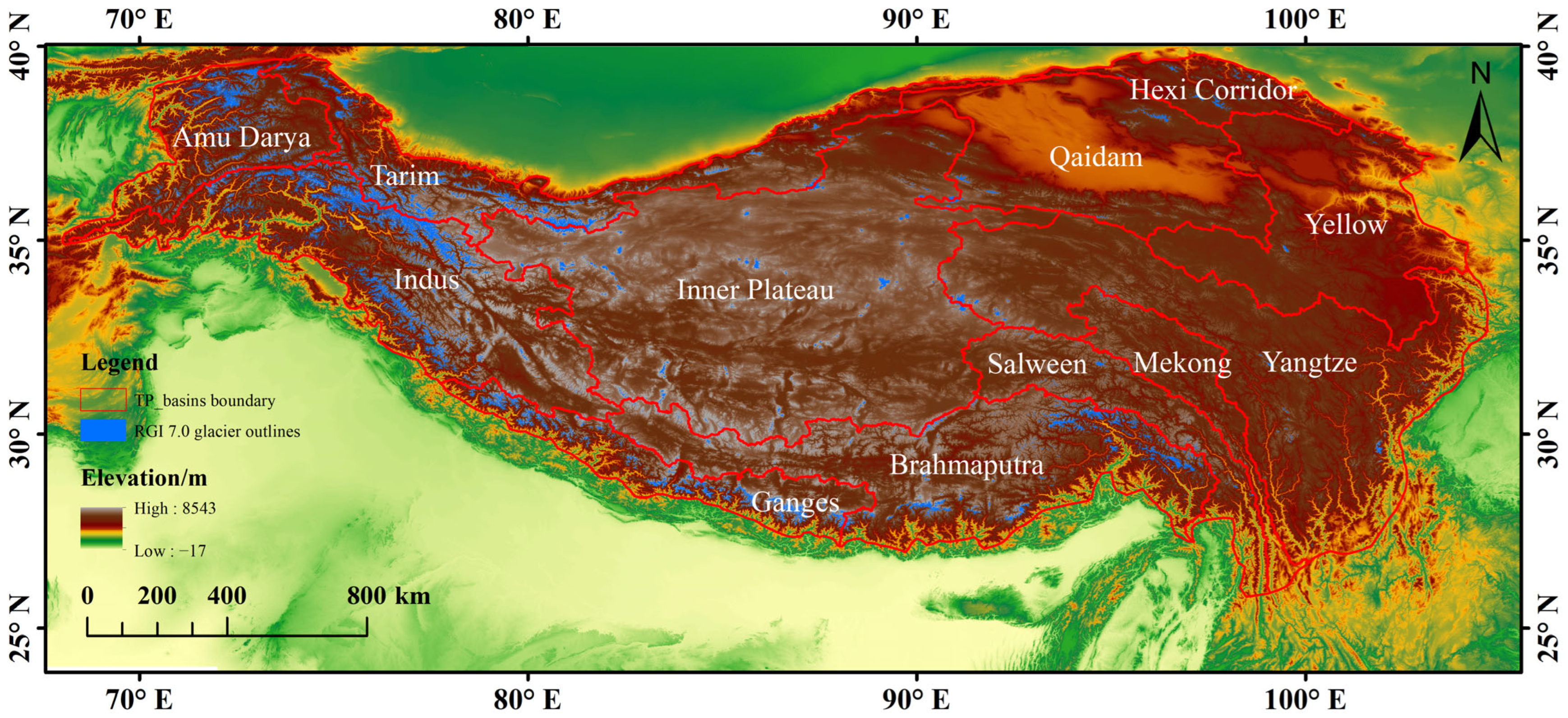
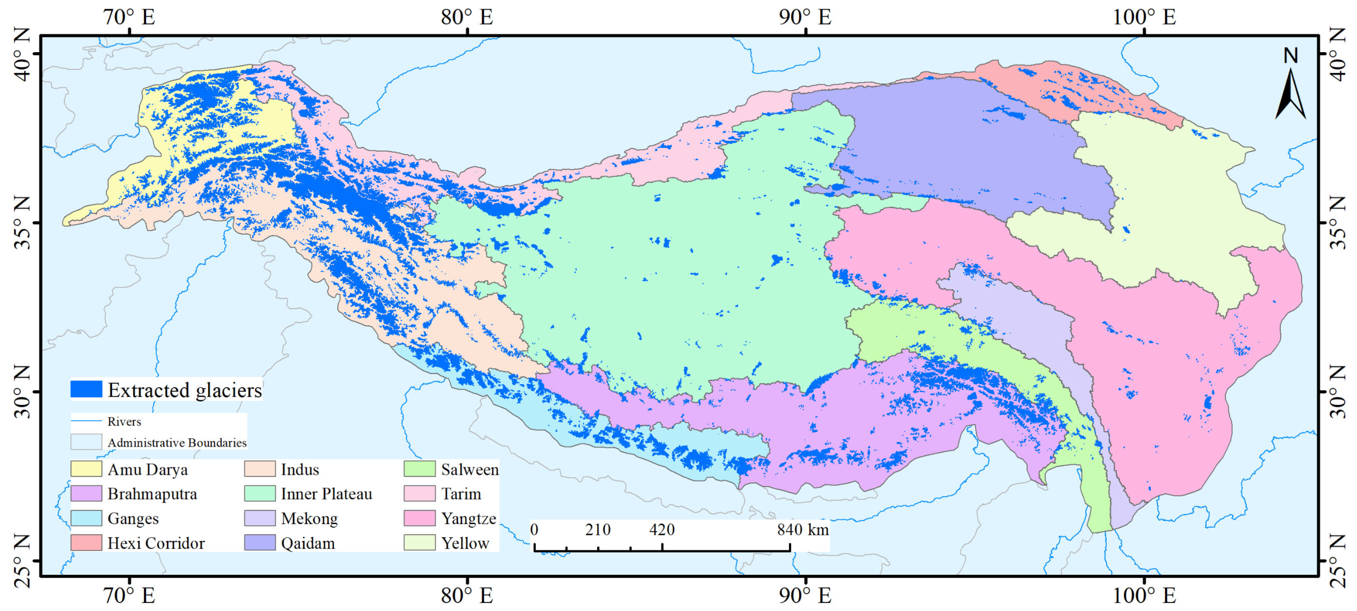
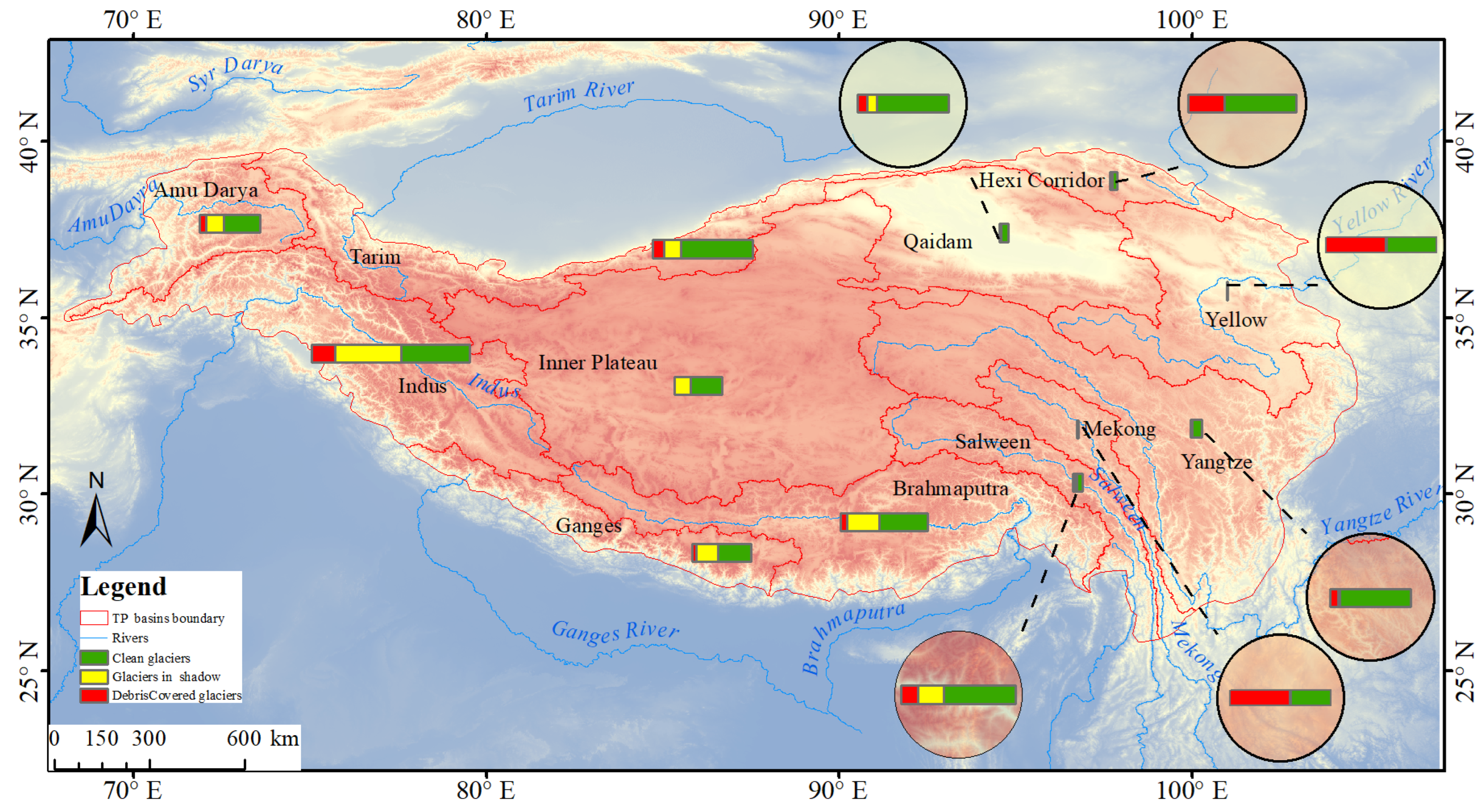
The Tibetan Plateau basin extends from 26°00′ to 39°47′N and 73°19′ to 104°47′E, covering an area of approximately 2.6 million km², with an average elevation exceeding 4000 m [25]; the overall terrain is high, with elevations higher in the northwest and lower in the southeast. The Tibetan Plateau spans multiple longitudes and latitudes and encompasses five climatic zones: from south to north, tropical, subtropical, plateau temperate, plateau subfrigid, and plateau frigid zones. The climate is diverse, characterized by thin air, dry and clean atmosphere with low humidity, strong solar radiation, and low temperature and pressure; the annual mean temperature is 1.6 °C; and the annual precipitation is 413.6 mm [26]. Temperature and precipitation are highly uneven in spatial distribution due to the blocking effects of high mountains. The region features distinct dry and wet seasons, with rainfall synchronized with periods of higher temperature. Winters are characterized by strong winds and cold, dry conditions. The Tibetan Plateau can be divided into 12 sub-basins [27], as shown in Figure 1.

Many mountain glaciers have developed within Tibetan Plateau basins, exhibiting pronounced spatial heterogeneity, with the Tarim, Indus, and Amu Darya basins being the most glacier-concentrated regions. Glacier identification in Tibetan Plateau basins still faces significant challenges. On the one hand, frequent seasonal snow is often confused with perennial glaciers, leading to considerable errors in traditional optical remote sensing during dry and wet season mapping. On the other hand, numerous debris-covered glaciers distributed in highly fragmented terrain, such as the Himalayas, exhibit spectral characteristics highly similar to those of surrounding rocks and soils, making automated boundary delineation extremely difficult. Furthermore, perennial cloud and fog cover in the southeastern Tibetan Plateau significantly restricts the usability of single-source optical observations. Therefore, utilizing microwave remote sensing with penetration capability (Sentinel-1 SAR) combined with multi-temporal optical features for glacier identification is of great significance for improving the automation level and accuracy of glacier monitoring in this region.

2.2. Data Sources and Sample Construction

2.2.1. Data Sources

The datasets used in this study include Sentinel-1 imagery, Sentinel-2 imagery, and DEM data, as well as glacier inventory and glacial lake inventory data, as shown in Table 1. Sentinel-1 SAR data were employed because they provide dual-polarization observations (VV and VH), which contain valuable backscattering information related to glacier surface roughness, moisture conditions, and debris cover characteristics. Meanwhile, Sentinel-2 multispectral imagery covering visible, near-infrared, and shortwave infrared bands [28] is employed to construct spectral and textural features. DEM data are derived from the ALOS DEM product with a spatial resolution of 30 m [29] to extract topographic factors such as elevation, slope, and aspect to support glacier identification.

In addition, the glacier inventory dataset (RGI v7.0) is used for model sample construction and accuracy validation, while the glacial lake inventory is employed to assist sample generation. All Sentinel-1, Sentinel-2, and DEM data are obtained from the GEE platform and undergo preprocessing steps, including radiometric calibration, cloud masking, and image mosaicking, to ensure data consistency and analytical accuracy.

RGI v7.0 was used as the primary glacier inventory dataset in this study. Although it represents the most up-to-date global glacier inventory, uncertainties remain in High Mountain Asia, particularly in regions characterized by extensive debris cover and complex topography. Previous studies have shown that debris-covered glacier boundaries are prone to omission and delineation errors because supraglacial debris exhibits spectral characteristics similar to surrounding moraines and bare-rock surfaces [30,31]. In addition, glacier inventories may still contain positional offsets and boundary uncertainties despite recent improvements introduced in RGI v7.0 [32].

Table 1. Data of the study area.

Data Type	Name	Data Source	Application
Remote sensing imagery	Sentinel-2A	GEE platform	Construction of optical and texture features
	Sentinel-1A		Construction of polarization features
	ALOS DEM		Construction of topographic features
Tibetan Plateau basin boundary dataset (2016)		National Tibetan Plateau Data Center [33]	Sub-basin delineation
Inventory datasets	Randolph Glacier Inventory, RGI v7.0	Data sourced from the National Cryosphere Desert Data Center (http://www.ncdc.ac.cn)	Accuracy validation and sample construction
	High Asia glacial lake inventory dataset

Table 1. Data of the study area.

Data Type	Name	Data Source	Application
Remote sensing imagery	Sentinel-2A	GEE platform	Construction of optical and texture features
	Sentinel-1A		Construction of polarization features
	ALOS DEM		Construction of topographic features
Tibetan Plateau basin boundary dataset (2016)		National Tibetan Plateau Data Center [33]	Sub-basin delineation
Inventory datasets	Randolph Glacier Inventory, RGI v7.0	Data sourced from the National Cryosphere Desert Data Center (http://www.ncdc.ac.cn)	Accuracy validation and sample construction
	High Asia glacial lake inventory dataset

All glacier boundary extraction results reported in this study correspond to the year 2020. Multi-temporal Sentinel-1 and Sentinel-2 observations acquired during 2020 were used for feature construction. Basin-specific valid temporal phases were determined according to image availability and cloud-cover conditions.

2.2.2. Sample Construction

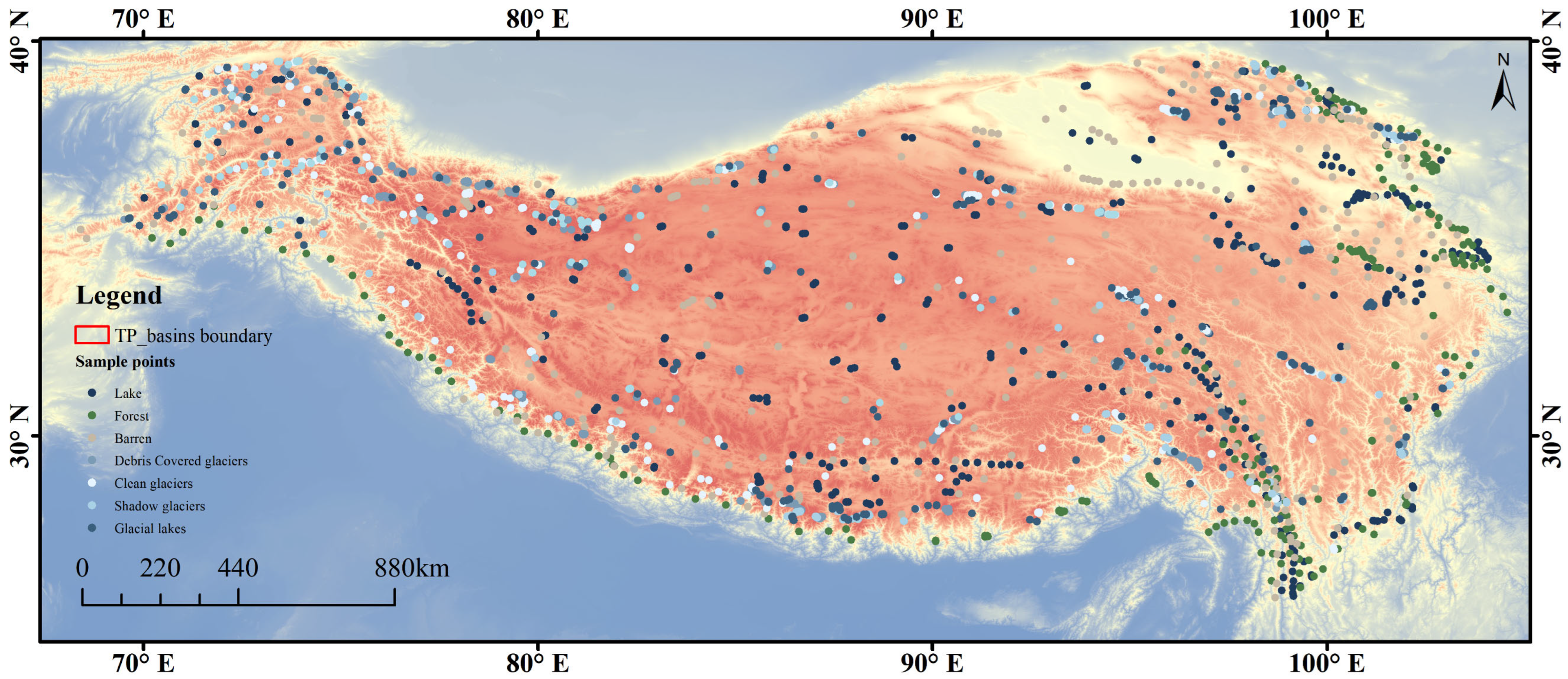
Reliable and accurate land cover sample data are crucial for the successful development of the model. The selection of sample data was based on composite imagery and supplemented by visual interpretation referencing the ESA WorldCover 10 m v100 global land cover dataset [34], Randolph Glacier Inventory (RGI 7.0) from the GLIMS program [32], and High Mountain Asia glacial lake inventory [35]. During sampling, strict adherence to randomness and uniformity principles was maintained to ensure that sample points of each category were evenly and randomly distributed across the study area. A total of 2366 independent samples—comprising clean glaciers (408), debris-covered glaciers (445), glaciers in shadow (344), glacial lakes (286), other water bodies (361), bare soil (302), and vegetation (220)—were compiled and partitioned into a training dataset (70%) and an independent validation dataset (30%) via a stratified random splitting strategy. The spatial distribution of the training and validation samples is shown in Figure 2.

To reduce the influence of spatial autocorrelation, glacier and non-glacier samples were distributed across multiple basins of the Tibetan Plateau. The training and validation samples were randomly partitioned from geographically diverse regions to improve the representativeness and generalization capability of the classifier. Nevertheless, some residual spatial dependence among neighboring samples may still exist and should be considered when interpreting the accuracy assessment results.

3. Automatic Glacier Identification Method

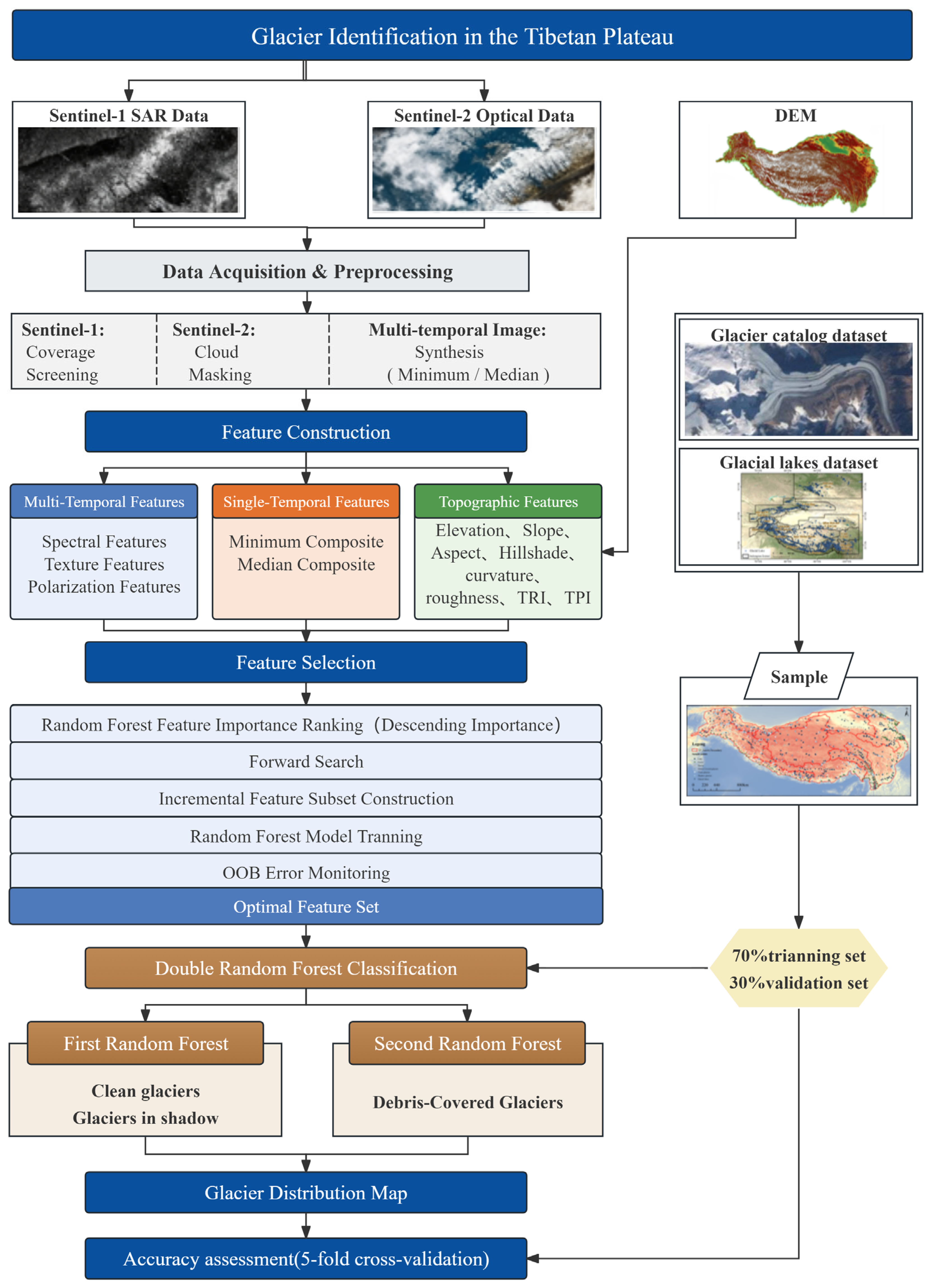
Based on glacier conditions, glaciers within the Tibetan Plateau are classified into three types: clean glaciers, debris-covered glaciers, and glaciers in shadow [36]. The core idea of glacier identification in this study is to integrate multi-source single- and multi-temporal features and then use a Double Random Forest (Double-RF) approach to progressively identify different glacier types. In the Double-RF framework, the first random forest extracts clean glaciers and glaciers in shadow, while the second random forest identifies debris-covered glaciers, thereby obtaining all glaciers distributed across the Tibetan Plateau.

The overall workflow of glacier identification is shown in Figure 3, where the main steps are as follows: (1) Data acquisition and preprocessing, where Sentinel-1/2 imagery is obtained, Sentinel-1 coverage is filtered, Sentinel-2 images are screened for cloud cover, and image compositing is applied to suppress the influence of snow and bare land on glacier boundary delineation. (2) Feature construction, including both multi- and single-temporal feature sets; multi-temporal spectral, texture, and polarimetric features are derived from multi-temporal Sentinel-1/2 imagery, while single-temporal features are constructed separately for the two classification stages using minimum and median compositing to obtain spectral and texture features, along with topographic features derived from DEM data. (3) Feature selection, where feature importance is calculated for both classification stages, and optimal feature subsets are selected based on feature importance and out-of-bag (OOB) error. (4) Double-RF glacier identification, which adopts a two-stage random forest classification strategy to progressively identify different glacier types; the first random forest focuses on distinguishing clean glaciers and glaciers in shadow based on spectral differences, while the second random forest specifically targets debris-covered glaciers.

Specifically, the Sentinel-2 imagery was selected exclusively from ice-free periods [37] (early June to early November). Meanwhile, although the multi-temporal feature construction for Sentinel-1 data incorporated year-round data across most basins, the subsequent feature selection process primarily retained images from the ablation season when seasonal snow cover was relatively minimal. This approach effectively mitigated the confounding effects of seasonal snow on glacier boundary identification.

3.1. Data Acquisition and Preprocessing

For SAR data, Sentinel-1 Ground Range Detected (GRD) imagery provided by the Google Earth Engine (GEE) platform was compiled. To address potential localized data gaps stemming from satellite revisit cycles and orbital configurations across the 12 sub-basins of the Tibetan Plateau, strict coverage screening was implemented to ensure complete data continuity for subsequent feature extraction.

To minimize the confounding effects of persistent cloud cover and seasonal snow on glacier boundary delineation, Sentinel-2 multispectral imagery was filtered to exclusively retain scenes acquired during the snow- and ice-free period (early June to early November) with a single-scene cloud cover threshold of less than 50%. This threshold was selected via a pilot trade-off analysis to guarantee sufficient spatial–temporal data coverage while optimizing computational efficiency.

Following cloud masking, all valid Sentinel-2 observations acquired during the snow- and ice-free season were aggregated on a pixel-by-pixel basis. In the first classification stage, minimum compositing was applied to each spectral band to suppress transient snow contamination and enhance clean-glacier detection. In the second classification stage, median compositing was adopted to reduce residual noise and represent the stable spectral characteristics of debris-covered surfaces.

The spectral characteristics of snow are very similar to those of clean glaciers but differ from those of debris-covered glaciers. Minimum compositing selects the lowest value of each pixel across the time series, effectively filtering out transient bright snow and thereby minimizing its impact on clean glacier extraction. Therefore, a minimum compositing approach was applied to the Sentinel-2 image collection in the first classification stage. In the second classification stage, median compositing was applied to Sentinel-2 imagery to eliminate transient noise and highlight the stable spectral signal of debris, enhancing the distinction from surrounding non-glacial bare rock areas and improving the extraction accuracy of debris-covered glaciers.

3.2. Feature Construction

3.2.1. Single-Temporal Feature Set

(1)

Spectral Features

All bands from Sentinel-2 are utilized, and band combinations are used to derive spectral indices beneficial for glacier extraction; Tasseled Cap Transformation (TCT) is applied to obtain the brightness, greenness, and wetness components. All spectral bands, along with brightness, greenness, wetness, and derived spectral indices, collectively form the spectral feature set. The spectral indices include Normalized Difference Vegetation Index (NDVI), Normalized Difference Water Index (NDWI), Normalized Difference Snow Index (NDSI), minimum band ratio indices (${\mathrm{Ratio}1}_{\min }$, ${\mathrm{Ratio}2}_{\min }$), and Band Difference Index (BDI), which are calculated as follows:

$$NDVI={\displaystyle \frac{{\rho }_{\mathrm{Red}}-{\rho }_{NIR}}{{\rho }_{\mathrm{Red}}+{\rho }_{NIR}}}$$

(1)

$$NDWI={\displaystyle \frac{{\rho }_{\mathrm{Green}}-{\rho }_{NIR}}{{\rho }_{\mathrm{Green}}+{\rho }_{NIR}}}$$

(2)

$$NDSI={\displaystyle \frac{{\rho }_{\mathrm{Green}}-{\rho }_{SWIR1}}{{\rho }_{\mathrm{Green}}+{\rho }_{SWIR1}}}$$

(3)

$${\mathrm{Ratio}1}_{\min }=\min \left({\displaystyle \frac{{\rho }_{\mathrm{Red}}}{{\rho }_{SWIR1}}}\right)$$

(4)

$${\mathrm{Ratio}2}_{\min }=\min \left({\displaystyle \frac{{\rho }_{NIR}}{{\rho }_{SWIR1}}}\right)$$

(5)

$$BDI={\rho }_{NIR}-{\rho }_{SWIR1}$$

(6)

In these formulas, ${\rho }_{\mathrm{Green}}$, ${\rho }_{\mathrm{Red}}$, ${\rho }_{NIR}$ and ${\rho }_{SWIR1}$ denote the reflectance values of the green (Green), red (Red), near-infrared (NIR), and shortwave infrared (SWIR) bands, respectively. Among them, the minimum band ratio indices Ratio1_min and Ratio2_min are used to reduce the influence of snow on glacier identification. BDI is used to distinguish glaciers in shadow, debris-covered glaciers, bare rock, and glacial lakes with similar spectral characteristics. The brightness, greenness, and wetness components derived from the TCT are used to distinguish debris-covered glaciers from spectrally similar rock and soil [38].

(2)

Texture Features

Remote sensing imagery often exhibits the phenomena of “same object with different spectra; different objects with similar spectra,” making glacier identification based solely on spectral features insufficient. Texture features represent image texture through the grayscale distribution of pixels and their surrounding spatial neighborhoods. The spatial distribution and patterns of pixel grayscale in texture reflect surface structure and roughness, which can be used to distinguish confusing land cover types and compensate for the limitations of relying solely on spectral information (color/brightness) for glacier identification. In 1973, Haralick [39] proposed the Gray-Level Co-occurrence Matrix (GLCM), which describes texture by analyzing the spatial relationships of grayscale values. In this study, the glcmTexture function provided by GEE is used to efficiently compute texture features based on GLCM, including contrast, correlation, variance, and difference moment.

(3)

Topographic Features

Topographic features are important indicators that reflect terrain undulation and surface morphology. Based on ALOS DEM data, we use the GEE platform to derive elevation and seven topographic features: slope, aspect, hillshade, curvature, roughness, terrain ruggedness index (TRI), and topographic position index (TPI).

(4)

Polarization Features

Sentinel-1 includes four imaging modes: stripmap (SM), extra wide swath (EW), wave mode (WM), and interferometric wide swath (IW) [40]. In this study, Sentinel-1 IW mode ground range detected (GRD) products are used, which include cross-polarization (VH) and co-polarization (VV), reflecting surface backscatter coefficients. Three polarimetric feature parameters, ${\sigma }_{VV}$, ${\sigma }_{VH}$, and ${\sigma }_{{\displaystyle \raisebox{1ex}{$VV$}\!\left/ \!\raisebox{-1ex}{$VH$}\right.}}$, are extracted from Sentinel-1 imagery for classification.

3.2.2. Multi-Temporal Feature Set

For the 12 sub-basins of the Tibetan Plateau, Sentinel-1 and Sentinel-2 imagery are selected on the GEE platform and composited at monthly intervals, resulting in 12 temporal composites. Temporal composites that do not fully cover each sub-basin or contain excessive cloud cover are removed, and valid temporal phases are retained; spectral, texture, and polarimetric features are then constructed within these valid phases to form the multi-temporal feature set for each sub-basin. The valid temporal phases for each sub-basin are listed in

Table 2. Valid temporal phases for each sub-basin.

Basin	Valid Sentinel-2 Temporal	Valid Sentinel-1 Temporal
AmuDayra	August, September, October	January to December
Brahmaputra	October, November	January to December
Ganges	September, October, November, December	January to December
Hexi Corridor	August, September, October	January to April, August to December
Indus	September, October	January to December
Inner	July, August, September, October	January to December
Mekong	August, October	January to December
Qaidam	August, September, October	January to December
Salween	August, October	January to December
Tarim	July, August, September	January to December
Yangtze	August, November	January to December
Yellow	August, September	January to April, August to December

. In Table 2, the Sentinel-1 and Sentinel-2 data are both from 2020.

3.3. Feature Selection

Multi-temporal features can fully leverage the dynamic temporal information contained in the imagery, improving the “same spectrum, different object” issue in classification results. However, using too many features to train a classifier not only complicates operations and significantly reduces processing speed but also decreases classification accuracy when the sample size is limited [41]. Hence, feature selection is essential to optimize model performance. In this study, feature importance and OOB error are used for feature selection. Feature importance evaluates the contribution of each input feature to the model’s predictive ability, allowing the removal of redundant or irrelevant features to enhance model performance. OOB error is an effective method to evaluate the model performance of random forests; it uses OOB samples for validation and provides an unbiased estimate of model generalization ability.

3.4. Random Forest Classification

Random Forest, introduced by Breiman, is an ensemble learning technique that employs decision trees as base classifiers and integrates bagging with the random subspace approach [42]. This algorithm can effectively handle high-dimensional data while avoiding overfitting. It has advantages under multi-feature, multi-class conditions, enabling the integration of various features for glacier identification across different land-cover conditions. Building a random forest model requires several parameters, including the number of decision trees (N) and number of variables (M) used for splitting the data. Typically, a small N may lead to underfitting, whereas a very large N can result in excessive computation. The value of M is usually determined as the square root of the number of input variables [43]. In this study, N was varied from 10 to 200 in increments of 1. After comparing the classification accuracy for each tree, the number of trees yielding the highest accuracy was selected as the model parameter.

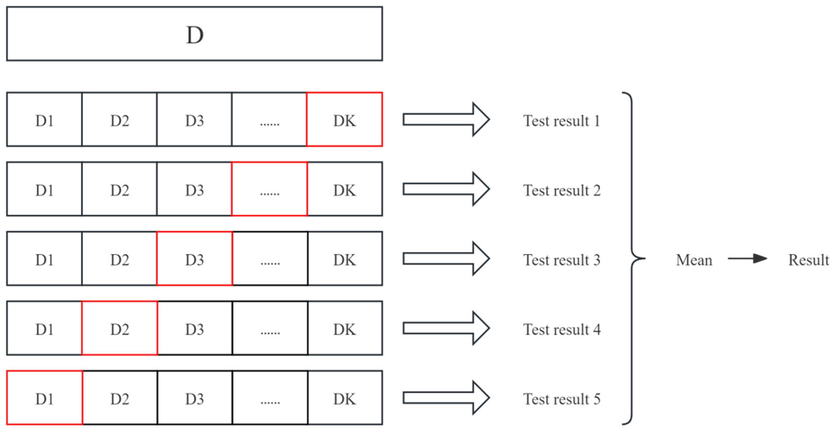
To assess model performance, approximately 70% of the samples were randomly assigned to the training set, while the remaining 30% were used for validation. A K-fold cross-validation approach was adopted, in which the training data were partitioned into non-overlapping subsets that collectively form the entire dataset; in each iteration, one subset was used for validation [44]. k was set to 5, meaning the dataset was split into five parts, with four used for training and one for validation in each round. Each iteration produces an associated accuracy metric. The mean accuracy across the five iterations was taken as the final estimate of model accuracy. The principle of K-fold cross-validation is illustrated in Figure 4.

4. Results and Analysis

4.1. Accuracy Evaluation of Feature Set Combinations

We construct an extensive feature set for the Yangtze River Basin; it includes traditional spectral features (18 single-temporal and 36 multi-temporal), texture features (4 single-temporal and 8 multi-temporal), and eight topographic features (e.g., elevation and slope). Notably, we fully exploit the polarimetric features of Sentinel-1, with as many as 36 multi-temporal variables capturing scattering variations throughout the year. This multi-source, multi-dimensional feature construction provides a solid data foundation for distinguishing debris-covered glaciers from spectrally similar rocks and soils.

To verify the advantage of combining single- and multi-temporal features, we control the number of random trees and use the Yangtze Basin as an example to evaluate the 5-fold cross-validation accuracy under three feature sets: single-temporal features, multi-temporal features, and their combination, with the results listed in

Table 3. Accuracy of different feature combinations in the Yangtze Basin.

Yangtze Basin		Single-Temporal Features	Multi-Temporal Features	Single-Temporal + Multi-Temporal Features
First classification	Number of tree	10
	Mean Accuracy	0.8201	0.7728	0.8328
	Mean Kappa	0.7805	0.7234	0.7968
Second classification	Number of tree	10
	Mean Accuracy	0.8599	0.7367	0.8829
	Mean Kappa	0.8059	0.6461	0.8380

. The 5-fold cross-validation results in Table 3 clearly demonstrate the superiority of feature fusion; in both classification experiments, the mean accuracy of single-temporal features (0.8201 and 0.8599) is significantly higher than that of purely multi-temporal features (0.7728 and 0.7367). This indicates that instantaneous spectral and texture information from single-temporal data still plays a dominant role in glacier identification. The fusion of single- and multi-temporal features achieved the highest accuracy. The mean accuracy increased to 0.8328 in the first stage and 0.8829 in the second stage, while the Kappa coefficient simultaneously rose to 0.8380. This demonstrates that multi-temporal features effectively compensate for the limitations of single-temporal imagery in identifying seasonal snow and cloud cover, thereby enhancing the generalization ability of the classifier. The accuracy improvement in the second classification after feature fusion (approximately 5% higher than in the first classification) is significantly greater than that of other combinations, validating the effectiveness of the proposed stepwise classification strategy.

In conclusion, single-temporal features provide fundamental land cover classification information, while multi-temporal features capture temporal variations in scattering and spectral responses, effectively suppressing environmental noise and enhancing class separability. This indicates that the combined “single-temporal + multi-temporal” feature set, under controlled conditions (with the number of random trees fixed at 10), achieves optimal accuracy and stability in glacier identification. Therefore, this optimal feature combination is adopted for glacier identification across all sub-basins of the Tibetan Plateau to ensure accuracy and scientific reliability at the basin-wide scale.

4.2. Accuracy Evaluation of Feature Selection

4.2.1. Feature Importance Analysis

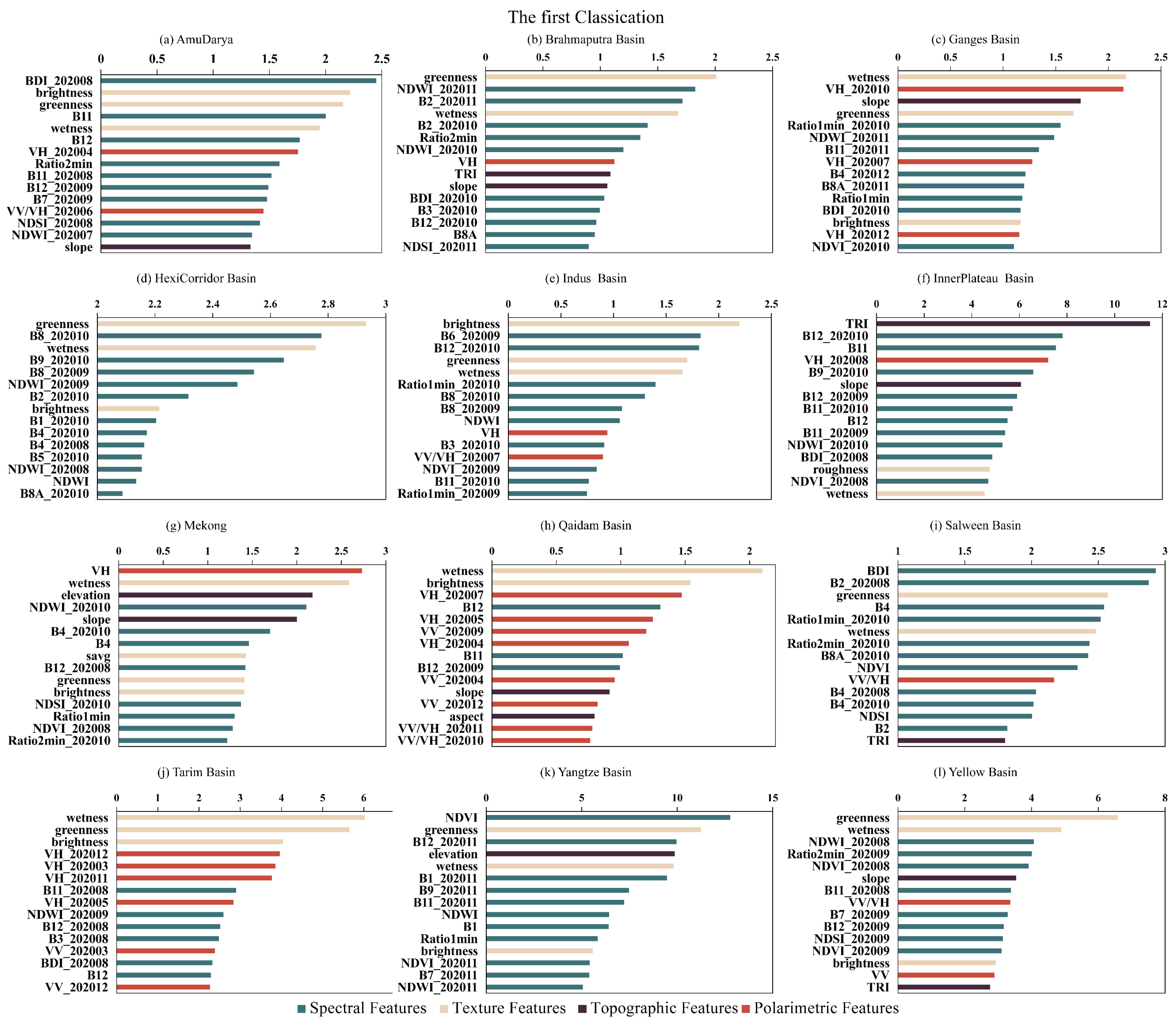
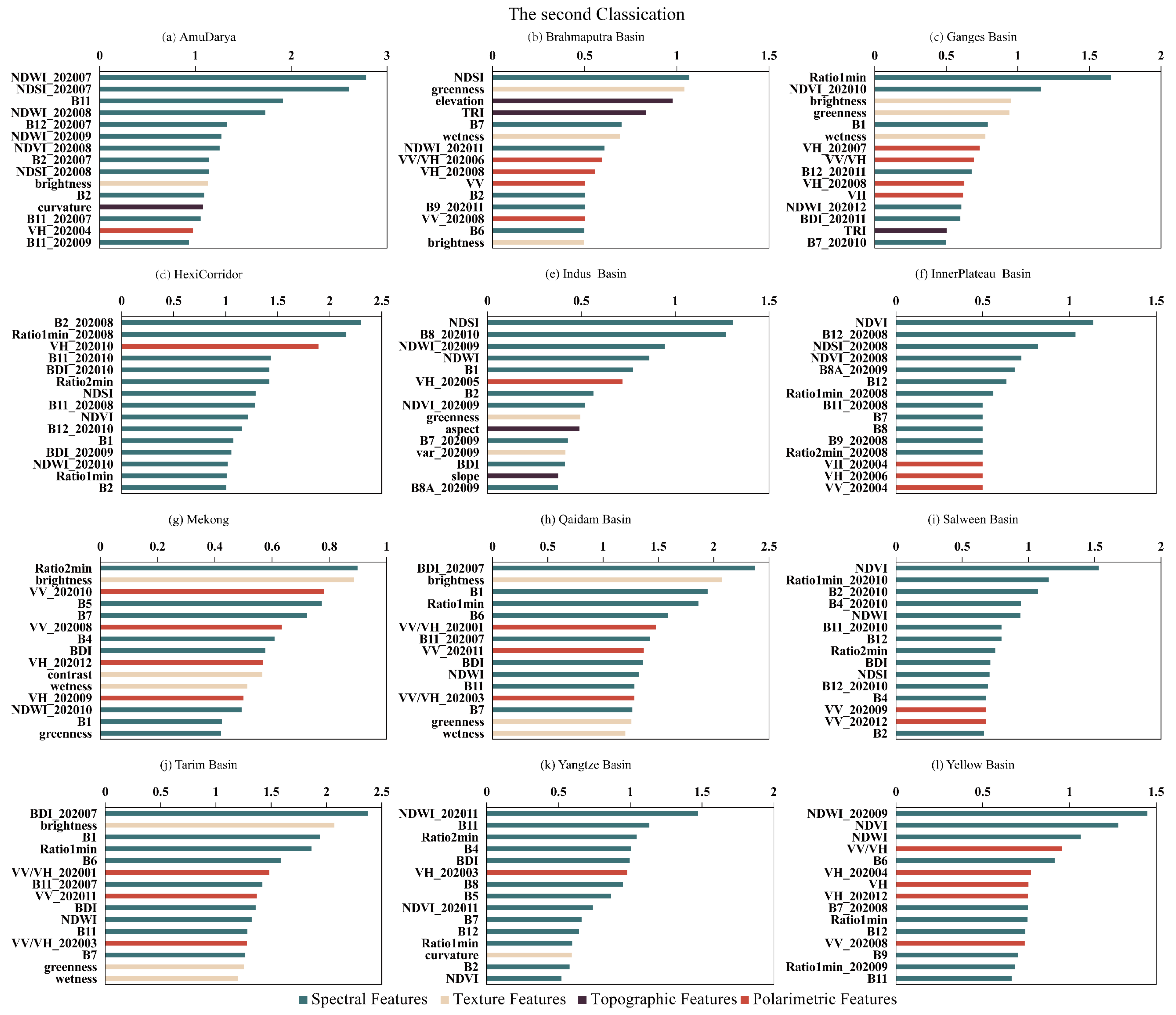
As mentioned for the random forest algorithm and feature construction, to eliminate redundancy among features and improve computational efficiency, we analyzed the importance of different variables in the feature sets of each sub-basin using the random forest algorithm, with the results shown in Figure 5 and Figure 6.

In the first classification, clean glaciers and glaciers in shadow were identified; Figure 5 shows the top-15 features by importance score in each sub-basin, revealing significant spatial heterogeneity in feature importance and reflecting the synergistic discriminative effects of different physical attributes. Texture features (brightness, greenness, and wetness) exhibit strong discriminative power across multiple basins. For instance, greenness is the most important feature in the Brahmaputra and Hexi Corridor basins, while wetness plays a dominant role in the Qaidam and Tarim basins. In addition, the incorporation of multi-temporal spectral information (e.g., BDI_202008, B8_202010) effectively captures seasonal phenological variations in glaciers, significantly improving the identification of glaciers in shadow. Meanwhile, polarimetric features (e.g., ${\sigma }_{VH}$, ${\sigma }_{VH}$_202010) show high discriminative importance in basins such as the Ganges and Mekong, effectively compensating for the lack of information in optical imagery over cloudy regions or shadowed areas.

In contrast, during the second classification for identifying debris-covered glaciers, the core features shift towards spectral index-driven variables. Indices such as NDSI, NDVI, and NDWI dominate across different basins. This indicates that distinguishing debris-covered glaciers from surrounding bare land relies more on subtle spectral differences. Multi-temporal features associated with specific months also show high importance in the second classification; in basins such as Amu Darya, Hexi, and Tarim, features from July to September are particularly influential, as the snow has largely melted, debris is fully exposed, and spectral characteristics are most stable. In contrast, basins such as the Ganges and Yangtze are mainly influenced by multi-temporal features from October to November, which avoid cloud interference from the summer monsoon season and utilize terrain shadows and moisture differences under lower solar elevation angles for identification.

Across the two glacier classification stages, feature importance varies significantly among different basins. The first classification is dominated by texture features (e.g., wetness, greenness, and brightness), whereas the second classification for debris-covered glaciers mainly relies on spectral indices (e.g., NDSI, NDVI, NDWI, and Ratio1min), with multi-temporal features contributing significantly in both stages. TRI, elevation, and slope generally show higher importance in the first classification than in the second, reflecting the distinctive topographic distribution of debris-covered glaciers (e.g., located in lower-elevation glacier tongues with specific slope ranges). The variation in feature importance across different basins reflects environmental heterogeneity in glacier coverage and debris conditions, which is closely related to glacier types and regional characteristics.

4.2.2. Optimal Feature Selection

Based on feature importance evaluation, although multi-dimensional features provide rich discriminative information, excessive feature dimensionality often introduces redundant noise, which not only increases computational complexity but may also lead to the “curse of dimensionality” under limited sample size, thereby reducing classification accuracy. Therefore, through feature selection, low-contribution variables are removed while maintaining model predictive capability, resulting in an optimal feature combination that balances generalization performance and computational efficiency.

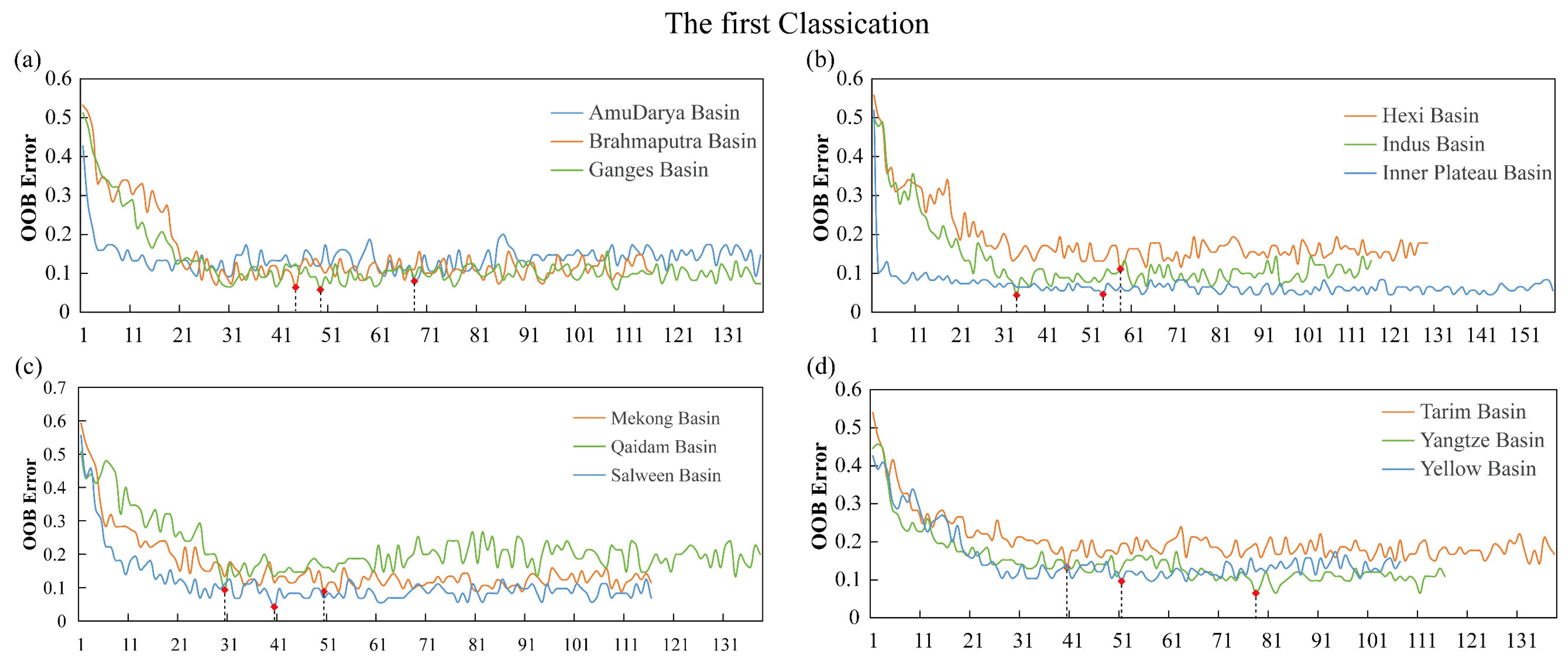
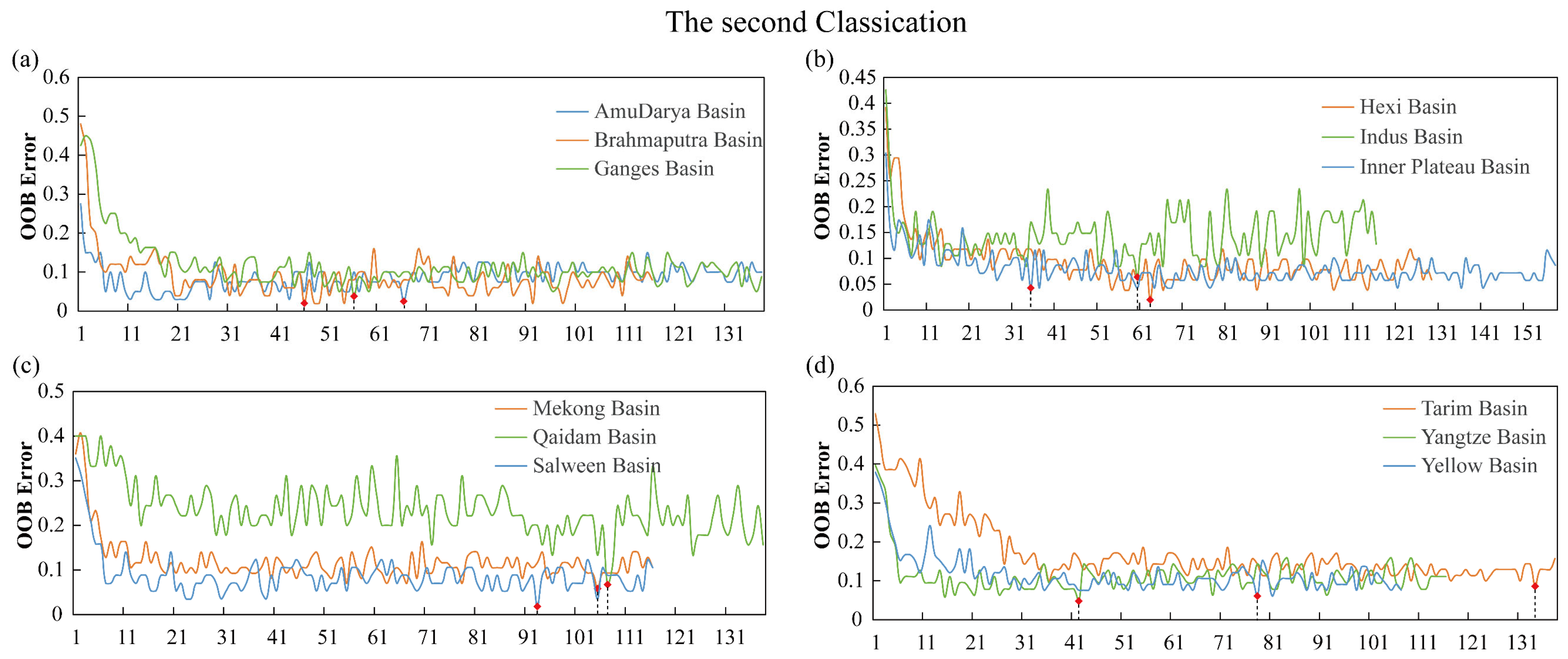
All feature variables are ranked in descending order according to their importance scores. A forward search strategy is adopted to incrementally add features and construct feature sets of different dimensions, with classification models built for each set; the OOB error is monitored and recorded, and the feature combination corresponding to the global minimum OOB error is selected as the optimal subset for each basin and used as input for the final glacier identification model. The relationship curves between the number of optimal features and error for each sub-basin are shown in Figure 7 and Figure 8.

In the first classification (clean glaciers and glacier in shadow identification), the number of features required to reach the minimum OOB error across basins shows strong convergence and consistency. The results show that, except for the Yangtze Basin (78 features) and Amu Darya (68 features), most basins (e.g., Indus, Salween, Qaidam, and Brahmaputra) have optimal feature subset sizes ranging from 28 to 58. This indicates that clean glaciers and glaciers in shadow have significant spectral differences, allowing high-accuracy classification without complex feature combinations. The top-60 features selected through feature importance evaluation contain sufficient discriminative information. This streamlined feature configuration not only ensures model generalization performance (as indicated by the minimum OOB error) but also effectively reduces overfitting caused by feature redundancy, demonstrating the efficiency of feature selection in this task.

In contrast, in the second classification, the relationship between feature number and OOB error exhibits strong heterogeneity and a polarized pattern. Some basins require significantly larger feature sets than in the first classification to reach the minimum OOB error, such as Tarim (134), Mekong (105), Qaidam (107), and Salween (93), indicating that the spectral responses of debris-covered glaciers are highly complex and diverse, requiring the combined effect of numerous features for accurate characterization. However, in some basins, such as Yangtze (42) and Inner Plateau (37), the optimal number of features is reduced. This pronounced polarization highlights considerable heterogeneity in the material composition, thickness, and environmental context of debris-covered glaciers among basins, resulting in markedly different optimal feature subsets in terms of both scale and structure. Accordingly, tailored feature selection at the basin scale is critical for this task and constitutes a fundamental prerequisite for developing models with high accuracy and strong generalization capability.

4.2.3. Accuracy Assessment of Optimal Features

The accuracy evaluation results of glacier identification using the double random forest model, based on the fusion and optimization of single- and multi-temporal features, are shown in

Table 4. Glacier identification accuracy in sub-basins.

Basins	First Classification			Second Classification
	Number of Trees	Mean Accuracy	Mean Kappa	Number of Trees	Mean Accuracy	Mean Kappa
AmuDarya	123	0.8790	0.8434	11	0.9357	0.9019
Brahmputra	21	0.9487	0.9359	157	0.9431	0.9230
Ganges	149	0.9423	0.9279	16	0.9514	0.9345
Hexi Corridor	38	0.8468	0.8055	56	0.9102	0.8735
Indus	23	0.8936	0.8690	10	0.9266	0.9049
Inner Plateau	19	0.9220	0.8957	11	0.9290	0.8781
Mekong	49	0.8909	0.8633	10	0.9560	0.9378
Qaidam	40	0.8876	0.8549	17	0.8024	0.7725
Salween	185	0.9214	0.8971	19	0.9478	0.9200
Tarim	36	0.8845	0.8455	118	0.8652	0.8092
Yangtze	63	0.8775	0.8509	42	0.9174	0.8848
Yellow	43	0.9824	0.9166	18	0.9052	0.8705

, including the random forest parameters (number of trees) for both the first and second classifications, along with their corresponding mean accuracy and mean Kappa coefficients.

Glacier identification across all basins achieved high accuracy, with mean accuracy exceeding 0.84, indicating that the adopted feature selection method has strong discriminative capability. In the first classification, basins with higher accuracy include the Yellow River Basin (Mean Accuracy = 0.9824), Brahmaputra Basin (0.9487), and Ganges Basin (0.9423), with corresponding Mean Kappa coefficients of 0.9166, 0.9359, and 0.9279, respectively, indicating good consistency in classification results. In contrast, the Hexi Corridor (Mean Accuracy = 0.8468) and Tarim Basin (0.8845) show relatively lower accuracy. In the second classification stage, overall accuracy improves compared to that in the first, with most basins achieving mean accuracy above 0.90; among them, the Mekong Basin (Mean Accuracy = 0.9560, Mean Kappa = 0.9378) and Ganges Basin (Mean Accuracy = 0.9514, Mean Kappa = 0.9345) perform best. Some regions, such as the Qaidam Basin, show slightly lower accuracy (Mean Accuracy = 0.8024).

Overall, the classification model after feature selection demonstrates high stability and reliability across different basins, indicating that the constructed feature set significantly improves glacier identification accuracy.

4.3. Results and Analysis of Glacier Extraction

4.3.1. Glacier Identification Results in the Tibetan Plateau

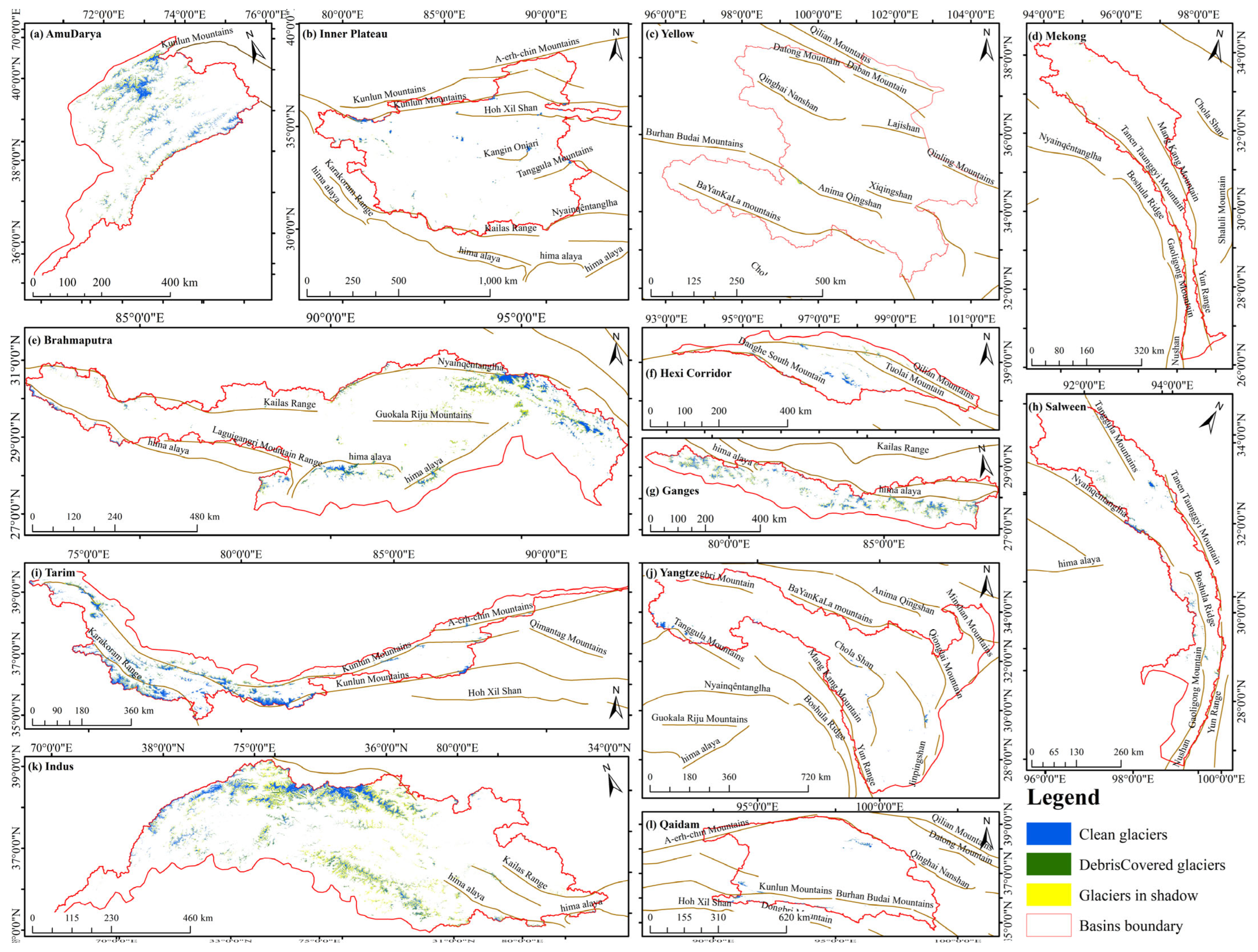
Glaciers in the Tibetan Plateau basin for the year 2020 were extracted using the Double-RF method based on the fusion of single- and multi-temporal features (Figure 9). Glaciers are mainly distributed in the western and southern parts of the Tibetan Plateau, concentrating in high mountainous regions, such as the Karakoram, Himalayas, and Kunlun Mountains. There are also significant differences in glacier distribution among basins, with the Indus Basin, Brahmaputra Basin, and Tarim Basin exhibiting the highest glacier density.

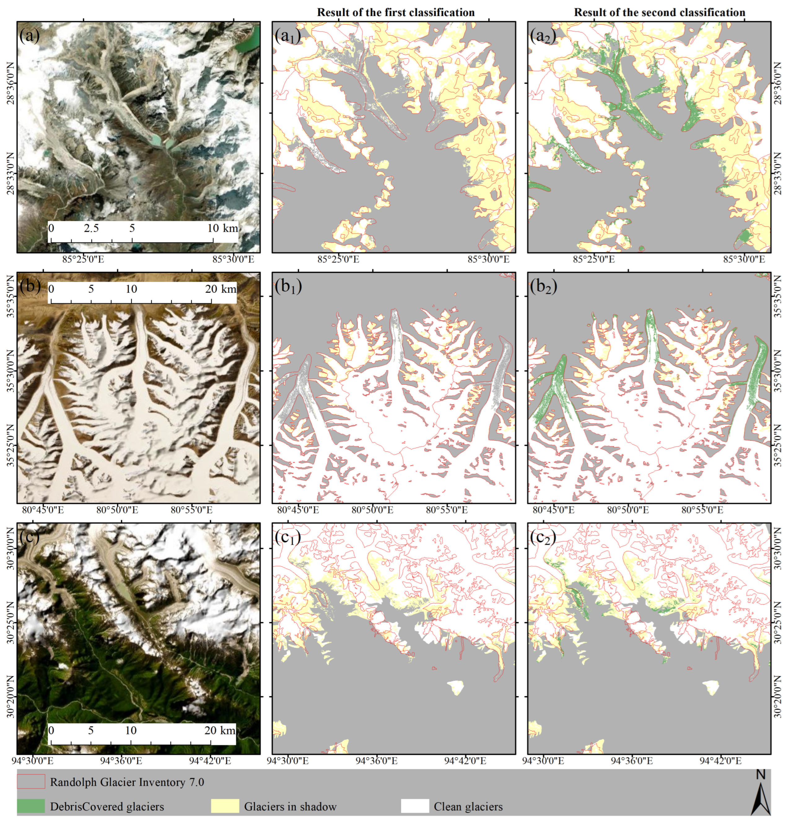
Figure 10 shows detailed glacier extraction results for the Tibetan Plateau; the first classification clearly distinguishes clean glaciers and glaciers in shadow, although some misclassification occurs at glacier boundaries and within shadowed areas. The second classification builds upon the first by identifying debris-covered glaciers, whose spatial extent shows high consistency with the boundaries of the RGI 7.0 inventory, resulting in more continuous and accurate glacier delineation. In addition, some glacier patches identified in this study are not recorded in existing inventory datasets. This demonstrates that multi-source and multi-temporal feature fusion improves the detection of glaciers with weak spectral responses while also indicating that existing inventories still have omissions in complex regions. Overall, the Double-RF method based on the fusion of single- and multi-temporal features demonstrates strong discriminative capability in complex-terrain and high-albedo regions, effectively capturing the spatial distribution characteristics of different glacier types.

Although existing glacier inventories (RGI 7.0) provide an important foundation for global glacier studies, they still exhibit uncertainties in delineating debris-covered glaciers and glaciers in shadow in complex terrain. Meanwhile, under rapid glacier evolution driven by climate change, traditional inventory datasets struggle to meet the requirements of large-scale dynamic monitoring in terms of timeliness and automated updating capability. In contrast, the Double-RF glacier identification method proposed in this paper, based on the fusion of single- and multi-temporal features, integrates multi-source remote sensing data and a hierarchical classification strategy to achieve automated and efficient extraction of different glacier types. This method not only maintains strong discriminative performance in complex-terrain and high-albedo regions but also demonstrates greater stability and continuity in identifying debris-covered glaciers and glaciers in shadow.

4.3.2. Comparative Analysis with Glacier Inventory Data

To systematically evaluate the performance of the Sentinel-1/2 data fusion method for glacier identification across different basins of the Tibetan Plateau, this study used the existing glacier inventory (RGI 7.0) as reference data, constructed pixel-level confusion matrices, and calculated metrics including Overall Accuracy (OA), Precision, Recall, F1-score, Intersection over Union (IoU), and the Kappa coefficient. The accuracy metrics for each basin are presented in

Table 5. Accuracy of glacier identification in each basin.

Basins	OA	Precision	Recall	F1-Score	IoU	Kappa
AmuDarya	0.9973	0.9958	0.9350	0.9645	0.9314	0.9631
Brahmaputra	0.9932	0.7437	0.9173	0.8214	0.6969	0.8180
Ganges	0.9986	0.9554	0.9662	0.9608	0.9245	0.9601
HexiCorridor	0.9990	0.9617	0.9325	0.9469	0.8992	0.9464
Indus	0.9990	0.9617	0.9325	0.9469	0.8992	0.9650
InnerPlateau	0.9996	0.9736	0.9528	0.9631	0.9288	0.9629
Mekong	0.9999	0.9257	0.9465	0.9360	0.8797	0.9359
Qaidam	0.9998	0.9717	0.9723	0.9720	0.9456	0.9719
Salween	0.9991	0.8457	0.9305	0.8861	0.7954	0.8856
Tarim	0.9984	0.9301	0.9886	0.9585	0.9203	0.9577
Yangtze	0.9998	0.9174	0.9825	0.9488	0.9026	0.9487
Yellow	0.9999	0.9239	0.9830	0.9525	0.9093	0.9524

.

In terms of precision, inland basins influenced by the westerlies (e.g., Qaidam, Hexi Corridor, Inner Plateau) perform significantly better than the Himalayan region, with Precision values all exceeding 0.96. Glaciers in inland basins generally have clean surfaces and regular morphology, with distinct optical and SAR signal characteristics, resulting in lower misclassification rates. In contrast, the Precision values for the Brahmaputra and Salween basins are only 0.7437 and 0.8457, respectively, which are significantly lower than those of other basins. This is mainly due to the high proportion of debris-covered glaciers and widespread terrain shadows in these regions, where glacier spectra are difficult to distinguish from bare rock in optical imagery, leading to higher false positives (FPs). In terms of recall, basins such as Tarim, Yangtze, and Qaidam all exceed 0.97, indicating that the model can effectively capture glacier boundaries in these regions. In contrast, the Recall values for the Amu Darya and Brahmaputra basins are 0.9350 and 0.9173, respectively; strong terrain occlusion and snow–rock mixed pixels contribute to more pronounced omission errors. The composite metrics (F1-score and IoU) show similar spatial patterns: except for the Brahmaputra basin, most basins have F1-scores between 0.94 and 0.97 and IoU values generally above 0.89, indicating high consistency between classification results and glacier inventory data in spatial extent and morphology. However, the Brahmaputra basin shows significantly lower F1-score (0.8214) and IoU (0.6969), demonstrating that extremely complex terrain, extensive debris-covered glaciers, and strong shadow effects significantly affect model performance.

Although significant differences exist among basins in class-sensitive metrics such as Precision and Recall, the overall accuracy in all basins exceeds 99%, indicating that the model performs well in distinguishing glaciers from non-glacier backgrounds. This indicates that the model performs robustly in glacier identification across the main Tibetan Plateau region, although there is still room for improvement in highly complex areas, such as the southern Himalayas.

4.3.3. Cross-Validation Using Independent Reference Samples

To further assess the robustness of the proposed Double-RF framework and address potential circular-validation concerns associated with glacier inventories, an independent validation was conducted using manually interpreted samples that were not involved in either model training or inventory generation. A total of 316 validation samples were collected, including 96 debris-covered glacier samples, 80 shadow glacier samples, 70 non-glacier debris/bare-rock samples, and 70 terrain-shadow non-glacier samples, as shown in

Table 6. Independent validation accuracy metrics.

Sample Type	Debris-Covered Glaciers	Shadow Glaciers	Non-Glacier Debris/Bare Rock	Terrain-Shadow Non-Glacier
Number	96	80	70	70
Overall Accuracy (%)	Kappa	Producer Accuracy (Glacier) (%)	Debris-covered glacier OA (%)	Glacier in shadow OA (%)
92.09	0.843	85.80	90.96	93.33

. All validation samples were independently derived through manual visual interpretation of high-resolution Google Earth imagery.

The independent validation yielded an overall accuracy of 92.09% and a Kappa coefficient of 0.843. The producer accuracy for glacier samples reached 85.80%, indicating that the proposed framework effectively avoided false glacier detections in spectrally confusing environments. Further analysis showed that the classification accuracy in debris-covered glacier areas reached 90.96%, whereas the accuracy in glacier in shadow regions reached 93.33%. These results demonstrate the strong capability of the Double-RF framework for distinguishing glaciers from surrounding debris-covered surfaces and terrain shadows.

5. Discussion

5.1. Analysis of Spatial Distribution Characteristics

Figure 11 illustrates the spatial distribution characteristics of different glacier types across the Tibetan Plateau and its surrounding major river basins. In general, glaciers are primarily distributed in high-elevation mountain ranges, showing significant regional heterogeneity and differences among basins. Spatially, clean glaciers are predominantly located in high-altitude, cold, and arid regions, including the Pamir–Karakoram ranges, central and western Himalayas, and Kunlun and Qilian Mountains. Glaciers in these regions are generally large in size, well-formed, and exhibit strong spatial continuity. Debris-covered glaciers are mainly concentrated on the southern slopes of the Himalayas, as well as in the Karakoram and Hindu Kush ranges. Glaciers in shadow are mainly found in high mountain-valley regions, such as the eastern Himalayas and northern foothills of the Gangdise Mountains. In terms of basin distribution, glaciers are most densely developed in the Tarim, Indus, and Ganges basins, with diverse glacier types; notably, debris-covered glaciers account for a significant proportion in the upper Indus region. The Brahmaputra basin contains a large number of glaciers, forming a belt-like distribution along the northern Himalayan foothills. By contrast, inland basins, such as the Qaidam Basin and Inner Plateau, contain only a limited number of primarily small and isolated clean glaciers. Northern marginal basins, such as the Yellow River and Hexi Corridor, contain only a small number of mountain glaciers.

The spatial distribution patterns and area proportions of different glacier types (clean glaciers, glaciers in shadow, and debris-covered glaciers) across basins of the Tibetan Plateau are shown in Figure 12. The glacier distribution across the Tibetan Plateau basins is jointly influenced by topography, climate, and moisture transport pathways, exhibiting significant regional differentiation. In addition, the area proportions of different glacier types vary significantly. Clean glaciers represent the primary glacier type in all basins, with especially high proportions in the Amu Darya, Yellow River, Yangtze, and Mekong basins. Debris-covered glaciers have higher proportions in western and southern basins (Indus, Ganges, and Brahmaputra), reflecting strong glacier activity, complex accumulation and ablation processes, and well-developed surface debris layers in these regions. Glaciers in shadow account for a relatively small proportion overall and are mainly found in areas with strong topographic shading or weak local radiation conditions, such as parts of the Inner Plateau and southern mountainous regions. The Indus and Brahmaputra basins have the largest total glacier areas and relatively high proportions of debris-covered glaciers, indicating that glaciers in these basins exhibit delayed and complex responses to climate change; this is mainly because thick debris layers reduce the direct thermal response to warming through an insulating effect, while the strong flow and accumulation processes of large glaciers partially offset ablation, resulting in glacier responses that differ markedly from those in other regions. In contrast, the Yellow River, Yangtze, and Mekong basins are dominated by clean glaciers, which are relatively smaller in scale and more sensitive to climate variability.

Overall, the glacier distribution across the Tibetan Plateau exhibits a pattern characterized by “greater abundance in the west than the east, higher concentration in peripheral regions than inland areas, dominance of clean glaciers, and significant debris-covered glaciers along the southern margins,” reflecting the combined influence of climate, topography, and hydrological conditions across basins.

5.2. Analysis of Elevation Distribution Characteristics

Historically, this region has experienced four glacial periods, resulting in moraine landforms distributed across different elevations. Therefore, elevation distribution reflects glacier changes across different periods; elevation, slope, and aspect data derived from the DEM were overlaid with glacier extraction results to analyze glacier spatial distribution characteristics.

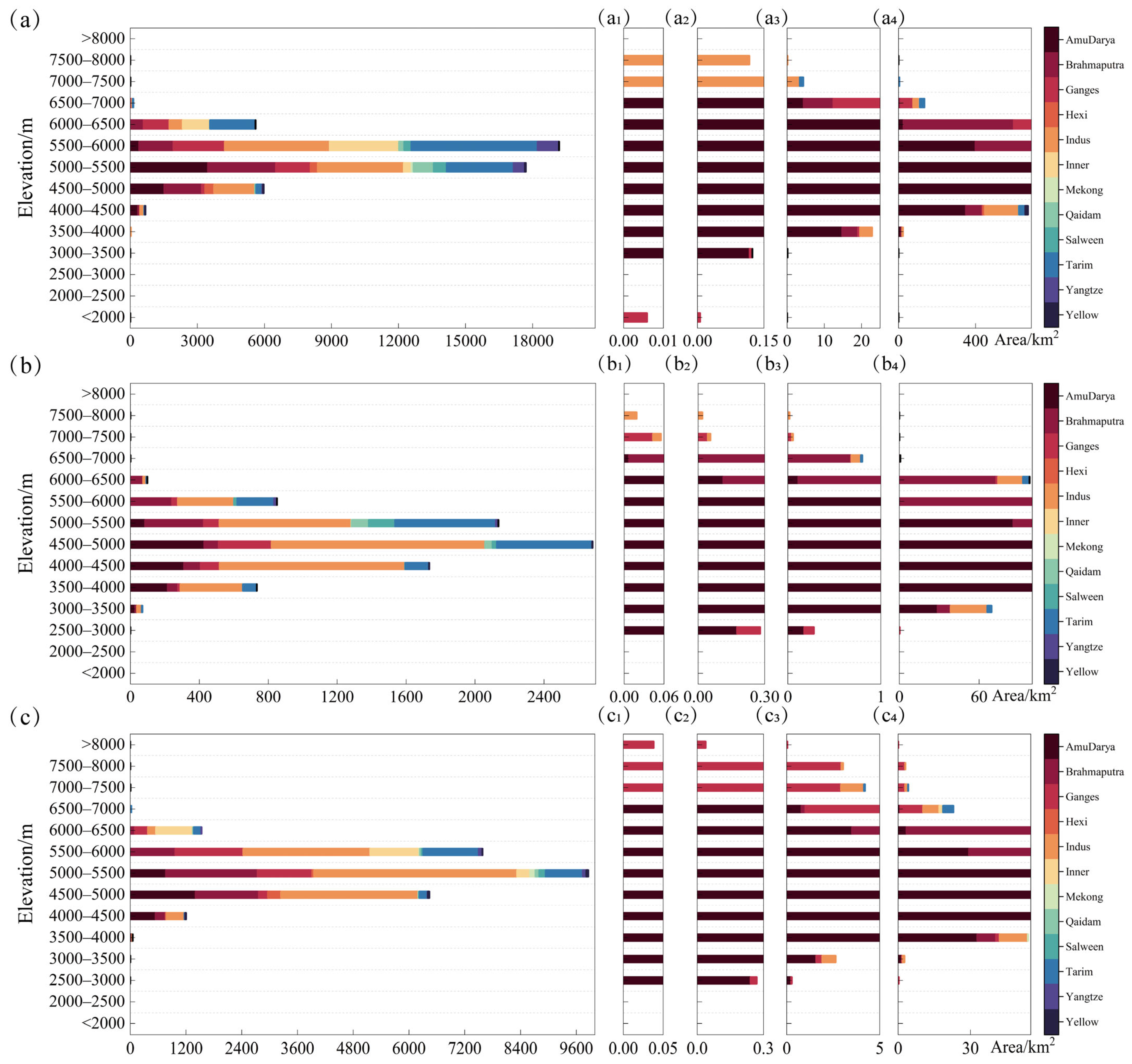
Figure 13 shows the elevation distribution characteristics of clean glaciers (a), debris-covered glaciers (b), and glaciers in shadow (c) across the Tibetan Plateau and its surrounding major basins. Clean glaciers (Figure 13a) are the most widely distributed across the Tibetan Plateau, with peak area mainly concentrated in the 5500–6000 m elevation band, followed by the 5000–5500 m range. Clean glaciers are mainly distributed in the Amu Darya, Indus, Inner Plateau, and Tarim basins, among which the Tarim basin has the highest proportion of clean glacier area, indicating favorable conditions for their development. By contrast, the Ganges and Brahmaputra basins maintain substantial clean glacier coverage above 6000 m, indicating higher glacier elevation limits driven by orographic uplift and ample precipitation. Enlarged views (a1–a4) show that clean glacier area decreases significantly at low elevations (<4500 m) and very high elevations (>7000 m), remaining only in a few basins, indicating high sensitivity to climate warming.

The elevation range of debris-covered glaciers (Figure 13b) is similar to that of clean glaciers, but their total area is significantly smaller. This type of glacier is mainly concentrated within the 4000–5500 m range, with a peak area at 4500–5000 m. The Amu Darya and Indus basins are the main concentration areas of debris-covered glaciers, indicating widespread development of debris layers on glacier termini in these arid inland basins. Enlarged views (b1–b4) further show that debris-covered glaciers are rare above 6500 m, while they still occur at mid–low elevations (3500–4000 m), indicating that thick supraglacial debris layers may partially suppress glacier ablation through thermal insulation effects, allowing debris-covered ice to persist at relatively lower elevations than clean glacier ice [45,46]. Compared with clean glaciers, debris-covered glaciers exhibit stronger spatial heterogeneity, reflecting their high dependence on energy conditions and glacier evolution stages.

Glaciers in shadow (Figure 13c) have relatively small areas and are mainly distributed at high elevations (4500–6000 m), with 5000–5500 m being the primary range. The Brahmaputra and Inner Plateau basins have relatively higher proportions of glaciers in shadow, indicating strong topographic relief and favorable shading conditions. Enlarged views (c1–c4) show a sparse distribution of glaciers in shadow above 6500 m and near absence below 4500 m, indicating their strong dependence on terrain shading. Compared with the other two glacier types, glaciers in shadow are smaller in scale but have relatively higher upper elevation limits, indicating a degree of environmental stability.

Overall, glaciers are mainly distributed between 4500 and 6500 m, with all three types showing clear elevation differentiation: clean glaciers have the highest upper limits, glaciers in shadow have the narrowest range, and debris-covered glaciers are most concentrated at mid-elevations. Significant differences in glacier types exist among basins; arid inland basins (e.g., Indus) are dominated by debris-covered and glaciers in shadow, whereas humid exoreic basins (e.g., Brahmaputra, Ganges) are dominated by clean glaciers. In general, the spatial distribution of glacier types is governed by the integrated influence of temperature gradients, precipitation regimes, and topographic shading effects.

5.3. Analysis of Slope Distribution Characteristics

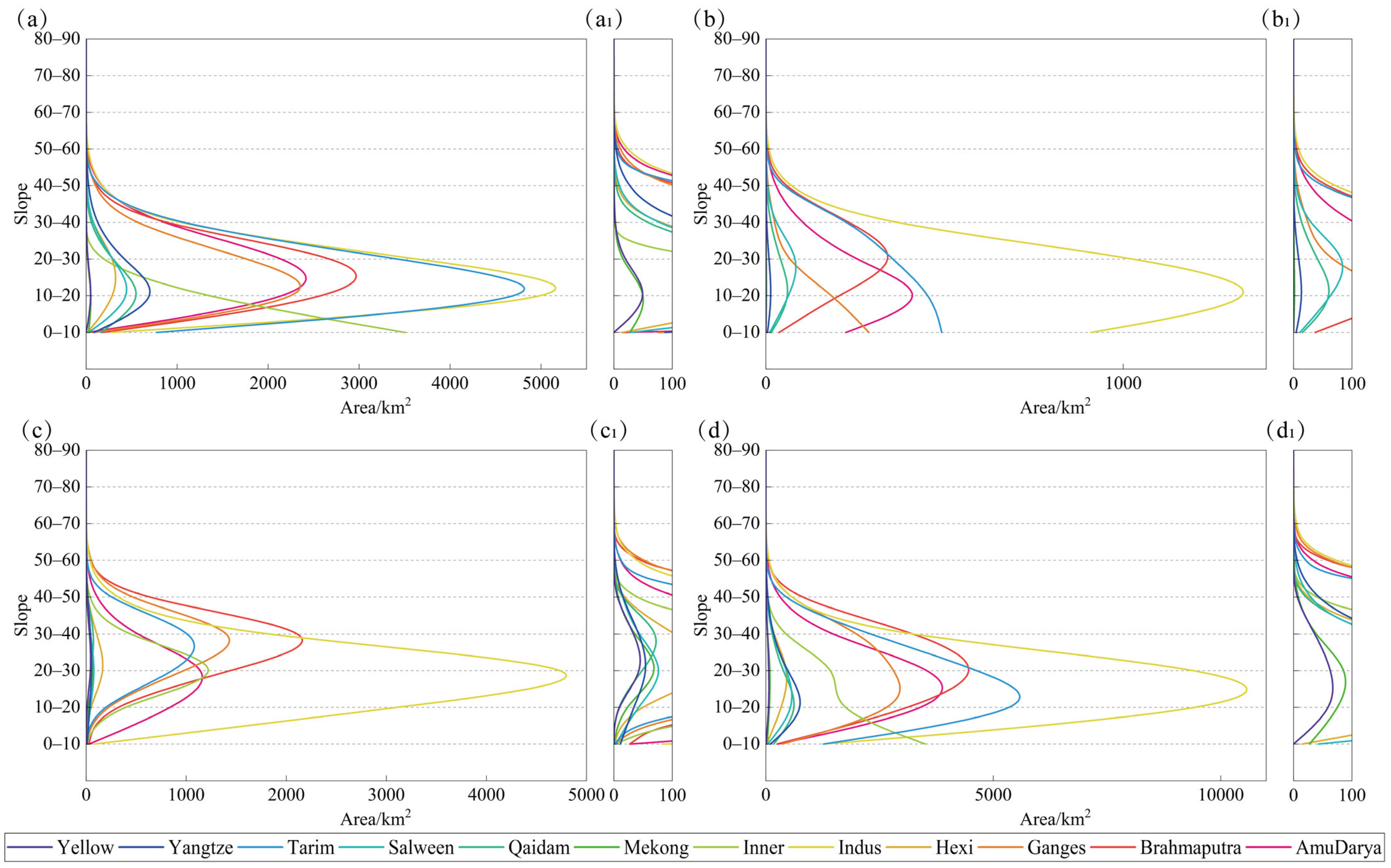
Figure 14 illustrates the area distribution of the three glacier types under different slope conditions. Panels a–c present the slope distributions of clean glaciers, debris-covered glaciers, and glaciers in shadow, respectively; a1–c1 are corresponding zoomed-in views. Panel d shows the slope distribution of all glaciers across the study area.

Clean glaciers (Figure 14a) have the highest area proportion within the 10–30° slope range, particularly in the Indus, Brahmaputra, and inland basins. This indicates that such glaciers mainly develop in mountainous valleys with moderate relief and well-extended glacier tongues. Slopes of 10–30° provide sufficient gravitational driving force for ice transport while avoiding frequent collapses and rapid mass loss associated with steeper slopes, thus favoring dynamic equilibrium and stability. As slope exceeds 30°, the area of clean glaciers decreases rapidly.

Debris-covered glaciers (Figure 14b) show a clear concentration towards lower slope ranges (0–20°). These glaciers are typically located at glacier termini or ablation zones, where terrain is relatively gentle. Glacier material is transported from steep accumulation zones to gentler ablation zones, where flow slows and debris from lateral and upstream sources accumulates. Therefore, debris-covered glaciers favor low-to-moderate slopes, which support stable debris cover and reduce ablation rates. The Tarim, Indus, Amu Darya, and Brahmaputra basins have significantly higher proportions of debris-covered glaciers, reflecting strong ablation and abundant debris supply in these regions.

The slope distribution of glaciers in shadow (Figure 14c) is similar to that of clean glaciers, but their peak shifts towards steeper slopes, with higher proportions in the 20–50° range, indicating development on shaded slopes or steep high-altitude terrain. Higher slopes indicate more complex terrain, providing better shading conditions, reducing solar radiation input, and favoring snow and ice accumulation and preservation. Their distribution is particularly prominent in the Brahmaputra and Indus basins, highlighting the strong influence of topographic shading and radiation conditions on their formation and preservation.

Overall, the glacier area on the Tibetan Plateau is highly concentrated within the 10–40° slope range, with 10–30° representing the most favorable slopes for glacier development and mass accumulation. Glacier area decreases significantly at very low slopes (0–10°) and steep slopes (>50°), reflecting the general pattern that low slopes hinder mass transport while steep slopes are unfavorable for ice stability and accumulation. The slope distribution characteristics show that clean glaciers tend to occur on moderate slopes, debris-covered glaciers concentrate on gentle slopes, and glaciers in shadow are mainly controlled by local topographic shading and steeper slopes. Differences among basins reveal significant spatial heterogeneity in glacier dynamic and thermal processes across the Tibetan Plateau.

5.4. Analysis of Aspect Distribution Characteristics

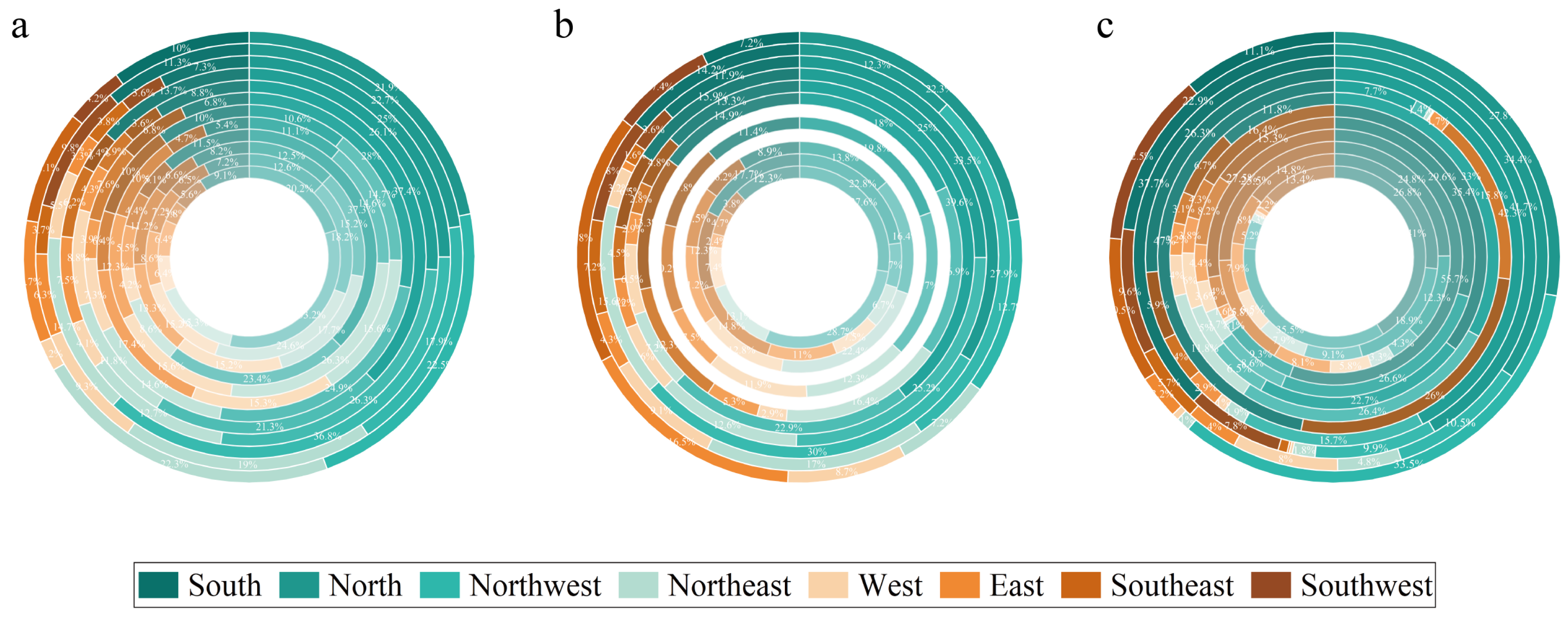
Figure 15 illustrates the area distribution of three glacier types across different aspects in the sub-basins of the Tibetan Plateau. Panels a, b, and c represent clean glaciers, debris-covered glaciers, and glaciers in shadow, respectively. The concentric rings from inner to outer denote the Amu Darya, Brahmaputra, Ganges, Hexi Corridor, Indus, Inner Plateau, Mekong, Qaidam, Salween, Tarim, Yangtze, and Yellow River basins. Different colors indicate dominant glacier aspects (South, North, Northwest, Northeast, West, East, Southeast, Southwest). Glacier aspect distribution is a key topographic factor controlling energy and mass balance, and its pattern is jointly influenced by solar radiation, local terrain shading, wind direction, and regional moisture transport.

Clean glaciers (Figure 15a) are mainly distributed on northeast- and east-facing slopes, particularly in the Tarim, Indus, Amu Darya, and Brahmaputra basins. Among them, the Tarim basin has the largest clean glacier area, mainly concentrated on northeast and north-facing slopes, indicating a strong dependence on low-temperature shaded environments in arid regions. In the Indus basin, influenced by both westerlies and monsoon systems, clean glaciers follow an aspect sequence of east > southeast > northeast, indicating that east-facing slopes receive moisture while avoiding intense afternoon radiation on west-facing slopes. The Brahmaputra basin shows a similar dominance of east- and northeast-facing slopes for clean glaciers. This indicates that clean glacier development is controlled by the balance between moisture transport pathways in accumulation zones (often from westerly or southwest flows forming snow accumulation on leeward east-facing slopes) and radiative–thermal conditions in ablation zones.

Debris-covered glaciers (Figure 15b) are highly concentrated on north- and northeast-facing slopes, with the most extensive development in the Indus and Tarim basins, where glacier area on north-facing slopes exceeds that on northeast-facing slopes. In contrast, debris-covered glaciers in monsoon-dominated basins such as the Brahmaputra are more dispersed, although north-facing slopes still account for a substantial proportion, highlighting the critical role of topographic shading in sustaining low-elevation debris-covered glaciers.

Glaciers in shadow (Figure 15c) are mainly distributed on north-, northeast-, and northwest-facing slopes; in most basins (Indus, Tarim, Brahmaputra, Ganges), north-facing slopes contribute the largest area. Particularly in the Brahmaputra and Ganges basins, the concentration of glaciers in shadow on north and northwest slopes contrasts sharply with the eastward distribution of clean glaciers. This confirms that glaciers in shadow are strictly controlled by topographic shading and depend heavily on shielding from solar shortwave radiation on shaded slopes.

Overall, glacier aspect distribution on the Tibetan Plateau shows that clean glaciers preferentially develop on east/northeast-facing slopes, where moisture and radiation are balanced; debris-covered glaciers are controlled by the northward extension of large glaciers and concentrate on north/northeast slopes; and glaciers in shadow strictly follow north-facing terrain shading patterns.

5.5. Limitations and Potential of Deep Learning-Based Glacier Mapping

The proposed Double-RF framework integrates Sentinel-1 and Sentinel-2 data and enables complementary exploitation of optical and SAR information. Furthermore, multi-temporal feature fusion effectively reduces the influence of seasonal snow, cloud contamination, and transient environmental noise. The hierarchical Double-RF strategy separately addresses clean glaciers, glaciers in shadow, and debris-covered glaciers, reducing spectral confusion and improving classification robustness. The robustness of the framework is further supported by the independent validation using manually interpreted samples, which achieved an overall accuracy of 92.09% and demonstrated reliable performance in both debris-covered glacier and terrain-shadow environments.

Although RGI v7.0 represents the most recent global glacier inventory, the acquisition dates of individual glacier outlines vary among regions and may not exactly coincide with the year 2020 used in this study. Such temporal inconsistencies may introduce minor uncertainties in rapidly changing glacier areas.

Although the proposed Double-RF framework achieved high glacier mapping accuracy, recent advances in deep learning provide promising opportunities for further improvement. Transformer-based architectures can effectively model long-range spatial dependencies and integrate heterogeneous multimodal information from optical, SAR, and topographic data [47]. Moreover, recent spectral-information compensation networks have demonstrated strong capabilities in preserving spectral characteristics while simultaneously extracting spatial contextual information [48]. Such approaches may further improve the identification of debris-covered glaciers and glaciers in shadow, where spectral confusion remains challenging. Future studies could explore the integration of Transformer-based multimodal learning frameworks with multi-temporal Sentinel observations for large-scale glacier mapping over the Tibetan Plateau. In addition, systematic benchmarking against classical threshold-based approaches (e.g., NDSI- and band-ratio-based methods), traditional machine learning methods, and emerging deep learning frameworks would provide a more comprehensive assessment of the strengths, limitations, and applicability of different glacier mapping strategies under complex mountain environments.

6. Conclusions

This study focused on high-precision glacier extraction over the Tibetan Plateau by integrating multi-source, multi-temporal active and passive remote sensing data from Sentinel-1/2, and a Double-RF automatic glacier identification method was proposed. Compared to conventional single-threshold and single-source classification approaches, this method effectively discriminates spectrally similar classes—including glacial lakes, bare rock, clean glaciers, debris-covered glaciers, and shadowed glaciers—with notable advantages in extracting shadowed and debris-covered glaciers. The method was implemented on the Google Earth Engine platform to achieve large-scale automatic mapping of different glacier types across the Tibetan Plateau, effectively enhancing the detection accuracy of clean, debris-covered, and in-shadow glaciers.

By constructing an optimal feature set and validating the accuracy across sub-basins, we successfully obtained high-precision spatial distribution patterns of the three glacier types across the Tibetan Plateau. The results demonstrate significant improvements in both accuracy and stability. The spatial distribution of glaciers exhibits patterns of “dense in the southwest and sparse in the northeast” and “dominance of clean glaciers with debris-covered glaciers concentrated along the southern and northern margins.” Integrated analysis of elevation, slope, and aspect indicates that different glacier types on the Tibetan Plateau exhibit distinct spatial differentiation: clean glaciers are mainly distributed at mid-to-high elevations (approximately 5000–6500 m) and gentle-to-moderate slopes (10–30°), preferentially on east- and northeast-facing slopes, reflecting stable development under the combined influence of moisture transport and radiation; debris-covered glaciers are concentrated at mid-to-low elevations (approximately 4500–5000 m) and low slopes (0–20°), primarily on north- and northeast-facing slopes, indicating dependence on ablation-zone conditions, debris supply, and terrain shielding; and glaciers in shadow are mainly located at mid-to-high elevations (approximately 5000–6500 m) and moderate-to-steep slopes (20–50°), concentrated on north- to northwest-facing shaded slopes, showing strong dependence on topographic shading and solar radiation blocking effects. The results reveal that regional climate gradients, energy balance, and topographic conditions jointly control the spatial differentiation of different glacier types, highlighting the strong spatial heterogeneity of glaciers on the Tibetan Plateau.

The glacier identification method proposed in this paper, which integrates multi-temporal Sentinel active and passive remote sensing data, significantly improves the automation and precision of glacier identification on the Tibetan Plateau and provides a practical approach for large-scale spatiotemporal glacier change monitoring. The results provide reliable data support and methodological reference for future glacier change studies and alpine water resource assessments, representing an important complement to existing glacier remote sensing techniques.

The proposed Double-RF framework provides an efficient and scalable solution for large-scale glacier mapping in complex mountain environments. By integrating optical, SAR, and topographic information, the framework effectively exploits the complementary strengths of multi-source remote sensing data and improves the detection of debris-covered glaciers and glaciers in terrain shadow, which are frequently omitted by conventional approaches. The results demonstrate the value of multi-source feature integration for automated glacier inventory generation and provide a transferable methodology for glacier mapping in other high-mountain regions. The generated glacier inventory can further support glacier change assessment, water resource management, glacier hazard monitoring, and climate-change impact studies across the Tibetan Plateau.

References

1. Latif, A.; Ilyas, S.; Zhang, Y.; Xin, Y.; Zhou, L.; Zhou, Q. Review on Global Change Status and Its Impacts on the Tibetan Plateau Environment. J. Plant Ecol. 2019, 12, 917–930. [Google Scholar] [CrossRef]
2. Xu, X.; Lu, C.; Shi, X.; Gao, S. World Water Tower: An Atmospheric Perspective. Geophys. Res. Lett. 2008, 35. [Google Scholar] [CrossRef]
3. Cook, K.L.; Andermann, C.; Gimbert, F.; Adhikari, B.R.; Hovius, N. Glacial Lake Outburst Floods as Drivers of Fluvial Erosion in the Himalaya. Science 2018, 362, 53–57. [Google Scholar] [CrossRef] [PubMed]
4. Nie, Y.; Pritchard, H.D.; Liu, Q.; Hennig, T.; Wang, W.; Wang, X.; Liu, S.; Nepal, S.; Samyn, D.; Hewitt, K.; et al. Glacial Change and Hydrological Implications in the Himalaya and Karakoram. Nat. Rev. Earth Environ. 2021, 2, 91–106. [Google Scholar] [CrossRef]
5. Shukla, T.; Sen, I.S. Preparing for Floods on the Third Pole. Science 2021, 372, 232–234. [Google Scholar] [CrossRef] [PubMed]
6. Paul, F.; Barrand, N.E.; Baumann, S.; Berthier, E.; Bolch, T.; Casey, K.; Frey, H.; Joshi, S.P.; Konovalov, V.; Bris, R.L.; et al. On the Accuracy of Glacier Outlines Derived from Remote-Sensing Data. Ann. Glaciol. 2013, 54, 171–182. [Google Scholar] [CrossRef]
7. Wu, L.; Li, X. Data Quality Evaluation for Database of the First Chinese Glacier Inventory. In Proceedings of the 2011 International Conference on Remote Sensing, Environment and Transportation Engineering, Nanjing, China, 24–26 June 2011; pp. 2067–2070. [Google Scholar]
8. Man, Q.X.; Guo, H.D.; Liu, G.; Dong, P.L. Comparison of Different Methods for Monitoring Glacier Changes Observed by Landsat Images. IOP Conf. Ser. Earth Environ. Sci. 2014, 17, 012127. [Google Scholar] [CrossRef]
9. Paul, F.; Bolch, T.; Briggs, K.; Kääb, A.; McMillan, M.; McNabb, R.; Nagler, T.; Nuth, C.; Rastner, P.; Strozzi, T.; et al. Error Sources and Guidelines for Quality Assessment of Glacier Area, Elevation Change, and Velocity Products Derived from Satellite Data in the Glaciers_cci Project. Remote Sens. Environ. 2017, 203, 256–275. [Google Scholar] [CrossRef]
10. Paul, F.; Bolch, T.; Kääb, A.; Nagler, T.; Nuth, C.; Scharrer, K.; Shepherd, A.; Strozzi, T.; Ticconi, F.; Bhambri, R.; et al. The Glaciers Climate Change Initiative: Methods for Creating Glacier Area, Elevation Change and Velocity Products. Remote Sens. Environ. 2015, 162, 408–426. [Google Scholar] [CrossRef]
11. Hall, D.K.; Riggs, G.A.; Salomonson, V.V. Development of Methods for Mapping Global Snow Cover Using Moderate Resolution Imaging Spectroradiometer Data. Remote Sens. Environ. 1995, 54, 127–140. [Google Scholar] [CrossRef]
12. Raghubanshi, S.; Agrawal, R.; Rathore, B.P. Enhanced Snow Cover Mapping Using Object-Based Classification and Normalized Difference Snow Index (NDSI). Earth Sci. Inform. 2023, 16, 2813–2824. [Google Scholar] [CrossRef]
13. Xin, C.; Sheng, Y. Enhancing Glacier Monitoring through Adaptive Smoothing of MODIS NDSI Time Series. Remote Sens. Lett. 2024, 15, 1047–1056. [Google Scholar] [CrossRef]
14. Xie, F.; Liu, S.; Gao, Y.; Zhu, Y.; Wu, K.; Qi, M.; Duan, S.; Tahir, A. Derivation of Supraglacial Debris Cover by Machine Learning Algorithms on the Gee Platform: A Case Study of Glaciers in the Hunza Valley. ISPRS Ann. Photogramm. Remote Sens. Spat. Inf. Sci. 2020, V-3-2020, 417–424. [Google Scholar] [CrossRef]
15. Zhen, L.; Wenxin, S.; Qunzhu, Z. Deriving Glacier Change Information on the Xizang (Tibetan) Plateau by Integrating Rs and Gis Techniques. Acta Geogr. Sin. 1999, 54, 263–268. [Google Scholar] [CrossRef]
16. Atwood, D.K.; Meyer, F.; Arendt, A. Using L-Band SAR Coherence to Delineate Glacier Extent. Can. J. Remote Sens. 2010, 36, S186–S195. [Google Scholar] [CrossRef]
17. Huang, L.; Li, Z.; Tian, B.; Zhou, J.; Chen, Q. Recognition of Supraglacial Debris in the Tianshan Mountains on Polarimetric SAR Images. Remote Sens. Environ. 2014, 145, 47–54. [Google Scholar] [CrossRef]
18. Alifu, H.; Vuillaume, J.-F.; Johnson, B.A.; Hirabayashi, Y. Machine-Learning Classification of Debris-Covered Glaciers Using a Combination of Sentinel-1/-2 (SAR/Optical), Landsat 8 (Thermal) and Digital Elevation Data. Geomorphology 2020, 369, 107365. [Google Scholar] [CrossRef]
19. Chu, X.; Yao, X.; Duan, H.; Chen, C.; Li, J.; Pang, W. Glacier Extraction Based on High-Spatial-Resolution Remote-Sensing Images Using a Deep-Learning Approach with Attention Mechanism. Cryosphere 2022, 16, 4273–4289. [Google Scholar] [CrossRef]
20. Kaushik, S.; Singh, T.; Bhardwaj, A.; Joshi, P.K.; Dietz, A.J. Automated Delineation of Supraglacial Debris Cover Using Deep Learning and Multisource Remote Sensing Data. Remote Sens. 2022, 14, 1352. [Google Scholar] [CrossRef]
21. Hu, Y.; Liu, L.; Huang, L.; Zhao, L.; Wu, T.; Wang, X.; Cai, J. Mapping and Characterizing Rock Glaciers in the Arid Western Kunlun Mountains Supported by InSAR and Deep Learning. J. Geophys. Res. Earth Surf. 2023, 128, e2023JF007206. [Google Scholar] [CrossRef]
22. Erharter, G.H.; Wagner, T.; Winkler, G.; Marcher, T. Machine Learning—An Approach for Consistent Rock Glacier Mapping and Inventorying—Example of Austria. Appl. Comput. Geosci. 2022, 16, 100093. [Google Scholar] [CrossRef]
23. Robson, B.A.; Bolch, T.; MacDonell, S.; Hölbling, D.; Rastner, P.; Schaffer, N. Automated Detection of Rock Glaciers Using Deep Learning and Object-Based Image Analysis. Remote Sens. Environ. 2020, 250, 112033. [Google Scholar] [CrossRef]
24. Mitkari, K.V.; Arora, M.K.; Tiwari, R.K.; Sofat, S.; Gusain, H.S.; Tiwari, S.P. Large-Scale Debris Cover Glacier Mapping Using Multisource Object-Based Image Analysis Approach. Remote Sens. 2022, 14, 3202. [Google Scholar] [CrossRef]
25. Li, C.; Su, F.; Yang, D.; Tong, K.; Meng, F.; Kan, B. Spatiotemporal Variation of Snow Cover over the Tibetan Plateau Based on MODIS Snow Product, 2001–2014. Int. J. Climatol. 2018, 38, 708–728. [Google Scholar] [CrossRef]
26. Wang, Y.; Lv, W.; Xue, K.; Wang, S.; Zhang, L.; Hu, R.; Zeng, H.; Xu, X.; Li, Y.; Jiang, L.; et al. Grassland Changes and Adaptive Management on the Qinghai–Tibetan Plateau. Nat. Rev. Earth Environ. 2022, 3, 668–683. [Google Scholar] [CrossRef]
27. Zhang, G.; Yao, T.; Xie, H.; Kang, S.; Lei, Y. Increased Mass over the Tibetan Plateau: From Lakes or Glaciers? Geophys. Res. Lett. 2013, 40, 2125–2130. [Google Scholar] [CrossRef]
28. Drusch, M.; Del Bello, U.; Carlier, S.; Colin, O.; Fernandez, V.; Gascon, F.; Hoersch, B.; Isola, C.; Laberinti, P.; Martimort, P.; et al. Sentinel-2: ESA’s Optical High-Resolution Mission for GMES Operational Services. Remote Sens. Environ. 2012, 120, 25–36. [Google Scholar] [CrossRef]
29. Tadono, T.; Ishida, H.; Oda, F.; Naito, S.; Minakawa, K.; Iwamoto, H. Precise Global DEM Generation by ALOS PRISM. ISPRS Ann. Photogramm. Remote Sens. Spat. Inf. Sci. 2014, II-4, 71–76. [Google Scholar] [CrossRef]
30. Herreid, S.; Pellicciotti, F. The State of Rock Debris Covering Earth’s Glaciers. Nat. Geosci. 2020, 13, 621–627. [Google Scholar] [CrossRef]
31. Thomas, D.J.; Robson, B.A.; Racoviteanu, A. An Integrated Deep Learning and Object-Based Image Analysis Approach for Mapping Debris-Covered Glaciers. Front. Remote Sens. 2023, 4, 1161530. [Google Scholar] [CrossRef]
32. Maussion, F.; Hock, R.; Paul, F.; Raup, B.; Rastner, P.; Zemp, M.; Andreassen, L.; Barr, I.; Bolch, T.; Kochtitzky, W.; et al. The Randolph Glacier Inventory Version 7. Zenodo 2023. [Google Scholar] [CrossRef]
33. Dataset of River Basins Map over the TP. 2016. Available online: https://data.tpdc.ac.cn/en/data/dff6b437-90a1-4729-8140-faafc544860f/ (accessed on 24 April 2026).
34. Zhai, J.; Xiao, C.; Feng, Z.; Liu, Y. Are There Suitable Global Datasets for Monitoring of Land Use and Land Cover in the Tropics? Evidences from Mainland Southeast Asia. Glob. Planet. Change 2023, 229, 104233. [Google Scholar] [CrossRef]
35. Wang, X.; Guo, X.; Yang, C.; Liu, Q.; Wei, J.; Zhang, Y.; Liu, S.; Zhang, Y.; Jiang, Z.; Tang, Z. Glacial Lake Inventory of High-Mountain Asia in 1990 and 2018 Derived from Landsat Images. Earth Syst. Sci. Data 2020, 12, 2169–2182. [Google Scholar] [CrossRef]
36. Miao, W.; Yongshun, H.; Dongshui, Z.; Xin, W.; Sangwangjie, G. Information Extraction Method of Debris-Covered Glaciers in Bomi County. Shandi Xuebao 2017, 35, 238–245. [Google Scholar]
37. Shi, X.; Wang, B.; Ma, Y.; Sun, L.; Li, W.; Lazhu; Hu, Z.; Zuo, H.; Li, X.; Chen, M. A Comprehensive Study on the Ice Freeze-Thaw Process in a High-Elevation Large Lake of the Tibetan Plateau. J. Geophys. Res. Atmos. 2025, 130, e2024JD042750. [Google Scholar] [CrossRef]
38. Shi, T.; Xu, H. Derivation of Tasseled Cap Transformation Coefficients for Sentinel-2 MSI At-Sensor Reflectance Data. IEEE J. Sel. Top. Appl. Earth Obs. Remote Sens. 2019, 12, 4038–4048. [Google Scholar] [CrossRef]
39. Haralick, R.M.; Shanmugam, K.; Dinstein, I. Textural Features for Image Classification. IEEE Trans. Syst. Man Cybern. 1973, SMC-3, 610–621. [Google Scholar] [CrossRef]
40. Yagüe-Martínez, N.; Prats-Iraola, P.; Rodríguez González, F.; Brcic, R.; Shau, R.; Geudtner, D.; Eineder, M.; Bamler, R. Interferometric Processing of Sentinel-1 TOPS Data. IEEE Trans. Geosci. Remote Sens. 2016, 54, 2220–2234. [Google Scholar] [CrossRef]
41. Bach, F. Breaking the Curse of Dimensionality with Convex Neural Networks. J. Mach. Learn. Res. 2017, 18, 629–681. [Google Scholar]
42. Breiman, L. Random Forests. Mach. Learn. 2001, 45, 5–32. [Google Scholar] [CrossRef]
43. Gislason, P.O.; Benediktsson, J.A.; Sveinsson, J.R. Random Forests for Land Cover Classification. Pattern Recognit. Lett. 2006, 27, 294–300. [Google Scholar] [CrossRef]
44. Kohavi, R. A Study of Cross-Validation and Bootstrap for Accuracy Estimation and Model Selection. In Proceedings of the 14th International Joint Conference on Artificial Intelligence, Montreal, QC, Canada, 20–25 August 1995. [Google Scholar]
45. Fyffe, C.L.; Woodget, A.S.; Kirkbride, M.P.; Deline, P.; Westoby, M.J.; Brock, B.W. Processes at the Margins of Supraglacial Debris Cover: Quantifying Dirty Ice Ablation and Debris Redistribution. Earth Surf. Process. Landf. 2020, 45, 2272–2290. [Google Scholar] [CrossRef]
46. Wang, F.-T.; Wang, L.; Li, Z.-Q.; Du, Z.-C.; Ming, J. Global Glacier Albedo Trends over 2000–2022: Drivers and Implications. Adv. Clim. Change Res. 2025, 16, 324–336. [Google Scholar] [CrossRef]
47. Yang, J.; Du, B.; Liu, R.; Mao, Z.; Zhang, L. Boosting Multimodal Remote Sensing Image Classification with Transformer-Based Heterogeneously Salient Graph Representation. IEEE Trans. Geosci. Remote Sens. 2026, 64, 5512117. [Google Scholar] [CrossRef]
48. Yang, J.; Du, B.; Xu, Y.; Zhang, L. Can Spectral Information Work While Extracting Spatial Distribution?—An Online Spectral Information Compensation Network for HSI Classification. IEEE Trans. Image Process. 2023, 32, 2360–2373. [Google Scholar] [CrossRef] [PubMed]
Figure 1. Spatial distribution of the Tibetan Plateau basin and its sub-basins.
Remotesensing 18 02148 g001
Figure 2. Distribution of sample points in the Tibetan Plateau basins.
Remotesensing 18 02148 g002
Figure 3. Flowchart of the glacier extraction method for the Tibetan Plateau.
Remotesensing 18 02148 g003
Figure 4. Illustration of the K-fold cross-validation principle.
Remotesensing 18 02148 g004
Figure 5. Ranking of feature importance in the first classification.
Remotesensing 18 02148 g005
Figure 6. Ranking of feature importance in the second classification.
Remotesensing 18 02148 g006
Figure 7. Relationship between feature number and OOB error in the first classification.
Remotesensing 18 02148 g007
Figure 8. Relationship between feature number and OOB error in the second classification.
Remotesensing 18 02148 g008
Figure 9. Glacier distribution in the Tibetan Plateau.
Remotesensing 18 02148 g009
Figure 10. Detailed glacier extraction results for the Tibetan Plateau: (ac) true-color base images; (a1c1) results of the first classification; (a2c2) results of the second classification.
Remotesensing 18 02148 g010
Figure 11. Distribution of different glacier types across sub-basins of the Tibetan Plateau.
Remotesensing 18 02148 g011
Figure 12. Area distribution of different glacier types on the Tibetan Plateau.
Remotesensing 18 02148 g012
Figure 13. Elevation distribution of different glaciers types: (a) Clean glaciers; (a1a4) local enlarged view of (a). (b) Debris-covered glaciers; (b1b4) local enlarged view of (b). (c) Glaciers in shadow; (c1c4) local enlarged view of (c).
Remotesensing 18 02148 g013
Figure 14. Areas of three types glaciers at different slopes: (a) Clean glaciers; (a1) local enlarged view of (a). (b) Debris-covered glaciers; (b1) local enlarged view of (b). (c) Glaciers in shadow; (c1) local enlarged view of (c). (d) All glaciers; (d1) local enlarged view of (d).
Remotesensing 18 02148 g014
Figure 15. Areas of three types of glaciers at different aspects: (a) Clean glaciers. (b) Debris-covered glaciers. (c) Glaciers in shadow.
Remotesensing 18 02148 g015