Article

Assessment of River Planform Dynamics in the Amazon Basin Using Sentinel-1 SAR Data (2017–2025)

Laboratory of Geo-Information Science and Remote Sensing, Wageningen University & Research, Droevendaalsesteeg 3, 6708 PB Wageningen, The Netherlands
*
Author to whom correspondence should be addressed.
Remote Sens. 2026, 18(13), 2075; https://doi.org/10.3390/rs18132075
Submission received: 15 May 2026 / Revised: 19 June 2026 / Accepted: 22 June 2026 / Published: 24 June 2026
(This article belongs to the Section Environmental Remote Sensing)

Highlights

What are the main findings?
  • Sentinel-1 C-band SAR data can derive basin-wide river planform metrics, including channel width, sinuosity and migration rate, across all Amazon tributaries from 2017 to 2025.
  • Centerline extraction enables river morphology metric extraction across sub-basins, revealing variations by flow pattern, basin position, and upstream–downstream pathway: lower sinuosity in anastomosing rivers, higher sinuosity in single-thread middle-basin rivers, wider channels in larger surface-water sub-basins, and heterogeneous migration rates independent of up- or downstream gradient.
What are the implications of the main findings?
  • The proposed planform river metric extraction method provides a framework for quantifying and monitoring river planform dynamics, especially in regions prone to cloud cover.
  • Sentinel-1 SAR can facilitate consistent, large-scale monitoring of geomorphological change in river planforms, aiding communities and biodiversity efforts.

Abstract

The Amazon Basin and its rivers play a vital role in regional biodiversity, the carbon cycle, and socio-economic security. Through erosion and deposition, river planforms change over time, affecting local infrastructure, food security, and changes to ecosystems. Long-term monitoring is essential for observing these dynamics. Synthetic Aperture Radar (SAR) provides a method to consistently map river planform dynamics across large areas because it is largely independent of atmospheric conditions. This study presents an approach for deriving river planform metrics across the entire Amazon Basin using Sentinel-1 C-band SAR data. This approach followed three main steps: water mask generation, validation of the data and river metrics extraction. Sentinel-1 imagery from 2017 to 2025 was composited into quarterly mean images, after which Otsu thresholding was applied to derive water classifications. Additional post-processing steps were applied to reduce terrain- and seasonal effects. The final water masks were divided into water-change classes, validated using stratified sampling and achieved an overall accuracy of 98.5%. Quarterly river planform metrics, including sinuosity, mean channel width and migration rate, were derived using channel centerline extraction, but due to a lack of in situ validation data the river metric values have not been validated. The resulting time series provide insights into how river planform changes across all Amazon sub-basins from 2017 to 2025 can be monitored using SAR-based methods. The results reveal spatial differences in river dynamics between tributaries, mostly depending on flow pattern, up- or downstream path and location in the upper, middle or lower Amazon Basin. These findings demonstrate the potential of SAR time series for monitoring large-scale river planform dynamics.

1. Introduction

The Amazon Basin is a key component in the global hydrological system, discharging around 15% of the world’s freshwater reserve into the ocean and providing a sediment discharge of 1200 tons/year [1,2]. Its rivers and floodplains house one of the most biodiverse areas in the world [3], with seasonal flooding transferring nutrients across the basin [1,4,5,6,7]. The Amazon rivers also power the eco-morphodynamic carbon pump, annually burying around 8.9 million tons of carbon through biomass transport into floodplains and the ocean [5,8,9]. In addition, the Amazon Basin regulates atmospheric circulation and moisture transport through intense evapotranspiration, driving heavy equatorial rainfall via convective precipitation [10,11]. Moreover, more than 30 million people depend on these river systems as a primary means of transportation, drinking water and food, while also facing risks from bank erosion, flooding and drought. This makes river channel stability critical not only for ecological integrity but also regional mobility, commerce and food security [1,5,6,8,12,13,14].
This hydrological system is dynamic and complex, mainly driven by seasonal flood pulses and sedimentary processes [3]. Seasonal inundation driven by the Inter Tropical Convergence Zone (ITCZ) is monomodal for the lowland areas with water rising up to 15 m at peak flooding season during March to May [7]. The frequency of extreme flooding events has however increased in recent years mainly due to anthropogenic climate change. These individual extremes can have great impact on the planform structure of rivers due to increased erosion and deposition [3,14]. After June water levels start receding, until eventually reaching the lowest water levels during August to October [5,15].
The region has highly active river systems that differentiate in planform between single-thread meandering and multi-channel anabranching (or anastomosing) patterns [3,4,5]. Lateral migration through erosion and deposition is the primary driving force of these changes. Meandering rivers are formed through high flow velocity on the outer bank of a river that exerts stress on the soil and causes particles to be swept away, leading to erosion. Contrary lower velocity streams on the inner bank of a river cause Earth particles in the water to settle and create sandbanks, leading to deposition [6,13,16,17,18]. These lateral bends can reconnect with the main channel, forming a cutoff. Flow then shifts to the shorter path, leaving the old loop as an oxbow lake [6]. Anastomosing or anabranching rivers are defined by multiple interconnected channels separated by stable vegetated islands that divide the waterflow [16]. These formations experience less erosion and deposition because avulsion processes are weaker, resulting in reduced lateral migration [4,5,18]. Given the highly dynamic nature of the Amazonian rivers and the river’s ecological, carbon-storage and socio-economic importance, monitoring spatiotemporal changes in river platforms on a large scale is essential.
Monitoring river dynamics across large and complex regions such as the Amazon has traditionally relied on accurate but labor-intensive, costly, and spatially limited field measurements, hampering large-scale monitoring of river dynamics [2,11,13]. With the introduction of freely accessible satellite data (e.g., Landsat), monitoring river planform dynamics has shifted from field-based observations to automated remote sensing, enabling large-scale monitoring [3,6,12,19]. Optical satellites such as the Landsat Program differentiate water from land using spectral indices based on strong absorption of near-infrared (NIR) and shortwave-infrared (SWIR) wavelengths by water, including the Normalized Difference Vegetation Index (NDVI) and Normalized Difference Water Index (NDWI) [4,6,20,21,22,23,24]. Despite their effectiveness, optical sensors are passive sensors that rely on reflected solar radiation and are therefore highly sensitive to atmospheric conditions [20,21,25]. During the Amazon’s tropical wet seasons, cloud cover is extensive and persistent leading to inconsistent observations and data gaps with optical sensors [25,26].
To overcome these obstacles, monitoring river dynamics in tropical regions has increasingly turned to Synthetic Aperture Radar (SAR), an active sensor that transmits and receives its own signal [27,28]. SAR uses microwaves that can penetrate clouds and acquire data independent of daylight, enabling consistent day-and-night observation regardless of atmospheric conditions [20,29,30]. Historically, using SAR data was hampered by inconsistent data archives and a lack of freely accessible data. This changed with the launch of Sentinel-1 in 2014, providing the first high resolution and freely accessible SAR data. SAR data is often used for water extent mapping because water is a specular reflector. When microwaves that have been transmitted hit the water, the signal scatters away from the satellite causing little of the original signal strength to return to the sensor [20,25]. This low backscatter signal contrasts with the higher return from the rough surrounding terrain (e.g., tree canopy or soil), making it well suited for water delineation [6]. The earliest methods of water classification using SAR relied on manual interpretation or simple radiometric thresholding [30,31]. Over time, more advanced algorithms emerged including automatic extraction like Otsu thresholding, change detection and fuzzy logic [1,21,25,26,28]. Current research is exploring superpixel segmentation and using statistical or machine learning models to produce accurate river masks [20,31,32]. With the addition of cloud computing like Google Earth Engine (GEE), large volumes of data can be processed more easily using external servers accessible through the internet [1,6,21,31].
Despite its advantages, SAR-based water mapping in the Amazon is subject to several environment-specific limitations that must be acknowledged. Sentinel-1’s C-band has limited penetration through dense vegetation, meaning that narrow channels and floodplains beneath closed canopy cover may be systematically under detected [1]. In addition, dry bare soil or recently cleared agricultural areas can also exhibit low backscatter due to their low dielectric properties, potentially leading to false water detections [28,30,32].
Despite growing interest in SAR-based hydrological applications, its use in river planform and morphodynamics analysis remains limited, especially in comparison to optical remote sensing. Most existing literature has relied on optical imagery due to its larger historical archive [33] and easier visual interpretations [28]. However, in regions such as the Amazon Basin, the inconsistent temporal availability of cloud-free images hampers continuous monitoring when solely relying on optical remote sensing data. Recent studies demonstrate that SAR provides more reliable temporal coverage in atmospherically complex regions, thereby outperforming optical remote sensing [27,28,30]. Its application in river morphodynamics, however, remains limited. Existing SAR-based studies have primarily focused on flood detection and open-water extent mapping (on both small- and large-scale) [1,21,25,26,28,30,32,34,35,36,37,38,39], rather than the systematic extraction of quantitative geomorphological metrics [6].
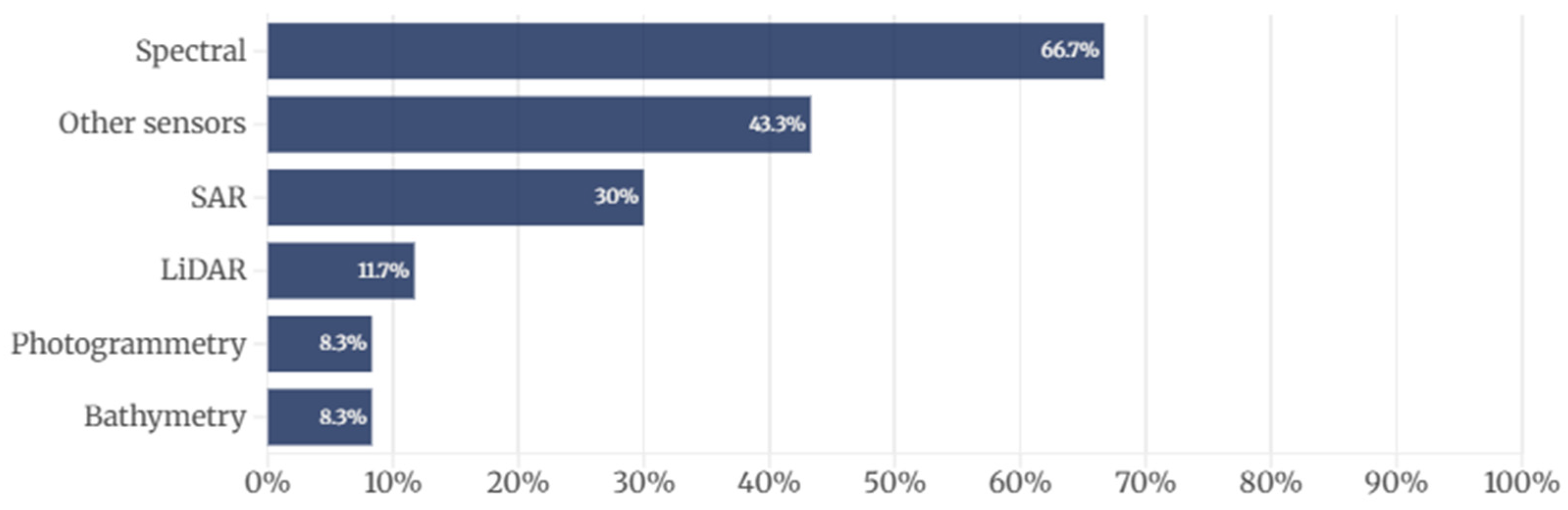
In addition, the field encompasses a wide range of river planform dynamics, leading to fragmented analytical approaches and a lack of consensus on the most suitable and effective metrics, particularly for those derived from SAR data. A structured literature review based on 60 recent studies on river planform dynamics (see Appendix A, for a full description of inclusion and exclusion criteria, search terms and database sources used in the semi-systematic review conducted via Web of Science), reveal that studies focus on many different combinations of river metrics depending on scale, data source and research focus, with meandering or migration, erosion, sinuosity, channel widening and deposition being the most commonly used dynamics (Figure 1).
At the same time, the review highlights a strong use of optical remote sensing data sources. More than two thirds of the analyzed studies used spectral imagery, while fewer than one third used SAR data (Figure 2). Aligning with a 2023 study by Nagel et al. that analyzed 800 papers regarding planform river dynamics, it was found that 80.7% of studies used a form of optical data, while only very few studies utilized SAR [6].
Moreover, the studies that used SAR data as a basis for planform river dynamic research have been confined to single tributaries or smaller regional basins [20,31,40,41]. While many small-scale [3,4,5,8,10,13,19,42] and large-scale [17,22,23,33,43,44,45,46] river metric analyses have been conducted before, these studies have all relied on spectral data. To this day, SAR remains understudied in the context of river morphodynamics and the consistent monitoring of river planform dynamics over a large-scale extent [29].
This study develops and evaluates a basin-wide framework for analyzing river planform dynamics across the Amazon Basin using Sentinel-1 SAR time series data from 2017 to 2025, advancing large-scale fluvial geomorphological change monitoring using SAR-based data. Quarterly water masks are produced, water-change classes are validated and automated centerline extraction is applied to quantify mean channel width, sinuosity, and migration rate across all Amazon sub-basins. It should be noted that not all high-frequency indicators identified in Figure 1 can be derived from static binary water masks alone. This study therefore focuses specifically on metrics that can be automatically extracted from quarterly SAR-derived water masks and addresses these four research questions:
  • Which river planform metrics are most commonly used in literature and suitable for extraction from SAR-based binary water masks at basin scale?
  • How accurately do Sentinel-1-derived quarterly water masks and water-change classes represent river dynamics relevant to planform analysis?
  • Can automated centerline extraction produce consistent estimates of width, sinuosity, and migration rate across the Amazon sub-basins from 2017 to 2025?
  • What spatial and temporal differences emerge among sub-basins and what do they reveal about the strengths and limitations of SAR-based monitoring?

2. Materials and Methods

2.1. Study Area

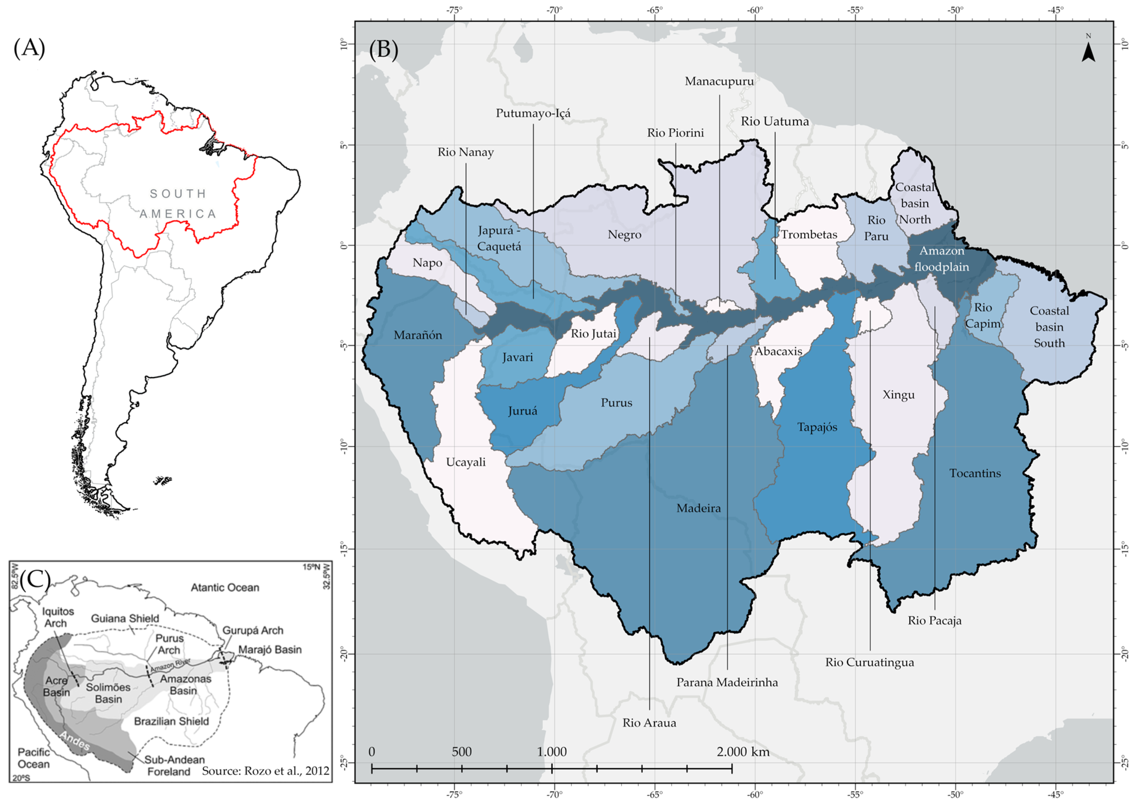
The Amazon Basin is located in northern South America and spans across parts of Bolivia, Brazil, Colombia, Ecuador, Peru, Suriname and Venezuela (Figure 3A). Although the hydrological area of the Amazon Basin is 6 million km2 [2], together with the Tocantins Basin and estuaries to the north and south of the Amazon’s mouth, the total area of the basin becomes almost 7 million km2. The Amazon Basin can be subdivided into 29 tributary sub-basins that are all connected to the main Amazon floodplain (Figure 3B) [7].
The Amazon Basin has been geologically developed on an intracratonic depression between the Andes mountain range to the west, the Guyana Shield to the north and the Central-Brazilian Shield to the south [5]. This depression is subdivided into four major areas: the Acre, Solimões, Amazonas and Marajó basins, which are separated from one another by the Iquitos, Purus and Gurupá arcs, respectively (Figure 3C) [11]. Sedimentary deposits within the basin range from Precambrian formations to more recent Holocene fluvial deposits. The current Amazon fluvial system evolved during the Neogene. During this time, tectonic processes and Andean uplift caused drainage pattern to form, establishing the present eastward-flowing river system [16].
Geomorphologically, the Amazon River systems are large alluvial rivers with most tributaries and the Amazon mainstem having low gradients, fine-grained sandy bed material and multichannel patterns, with median bed sediment sizes ranging between 0.13 and 0.5 mm and having a predominantly Andean sediment source. The Amazon mainstem and the biggest tributaries Negro and Madeira have predominantly anabranching planforms. The other smaller tributaries, mostly positioned in the middle or downstream regions have a meandering planform [47].

2.2. Data

2.2.1. Sentinel-1

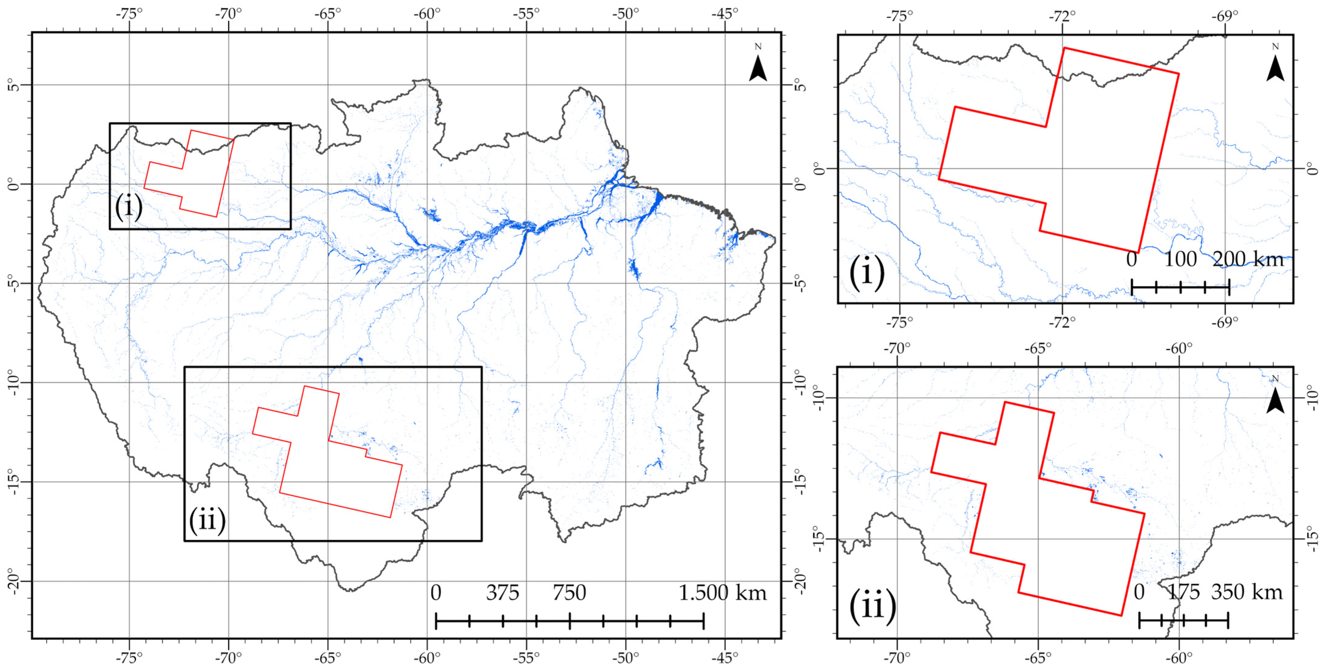
SAR data from the Sentinel-1 mission were used to extract surface water extent [48]. All available Ground Range Detected (GRD) images in the GEE (version 24 March 2026) catalogue were collected between 1 January 2017 and 31 December 2025, in Interferometric Wide (IW) swath mode and VH polarization. The imagery has a 10 m × 10 m pixel spacing with some pre-processing applied by ESA prior to the ingestion in the GEE catalogue including the application of GRD border noise removal, thermal noise removal, radiometric calibration and terrain correction using SRTM [49]. Both ascending and descending orbits were retrieved with a revisit time of up to 3 days using both Sentinel-1A and Sentinel-1B for the period 2017 to 2021. After the failure of Sentinel-1B in 2021 there was a recorded revisit time of up to 6 days during the period when only Sentinel-1A was active. During this period, several gaps in the data have occurred with missing data values for parts of the Japurá-Caquetá, Madeira and Negro sub-basins (Figure 4). A total of 22.133 ascending and 65.121 descending images were collected.
Additional pre-processing steps were applied to the Sentinel-1 GRD data, including border noise masking and temporal composite generation. The additional border noise masking was applied to remove artifacts from overlapping orbit paths, using an incidence angle filter that excluded values outside 30.74–45.04°, following Mullissa et al. [50]. Additionally, temporal composites (3-month intervals) for each year were generated to mitigate the effect of speckle by computing the mean of all available Sentinel-1 images within each period, totaling to 36 images.

2.2.2. ESA WorldCover

ESA WorldCover 10 m v200, is a global landcover dataset providing eleven landcover classes at 10 m × 10 m resolution [51]. The dataset is based on Sentinel-1 GRD and Sentinel-2 Level 2A products [52]. This data was used for landcover filtering and accessed using the GEE catalogue.

2.2.3. NASA SRTM

The Shuttle Radar Topography Mission (SRTM) by NASA is a Digital Elevation Model (DEM) providing global elevation data [53]. The dataset is based on single-pass interferometry data that uses two antennas with different angles to collect radar data with a resolution of 90 m × 90 m. This dataset is from 2007 and has an improved spatial resolution version of 30 m × 30 m that was used in this study [54]. This data was used for terrain artifact filtering and accessed using the GEE catalogue.

2.2.4. Major Amazon Regional and Tributary Basins BL1 and BL2

Regional and tributary Amazon Basin polygons were created by Venticinque et al. [7]. The dataset delineates drainage basins boundaries by using SRTM to calculate flow direction and flow accumulation rasters. Basin Level 1 (BL1) includes regional drainage polygons such as the full Amazon Basin and its estuaries. Basin Level 2 (BL2) defines major Amazon tributary basins larger than 100.00 km2 whose main stems flow into the Amazon River. These basins are used to define this study’s research areas.

2.2.5. PlanetScope Global Quarterly Visual Mosaics (Q3 Product)

PlanetScope global quarterly mosaics from PlanetLabs are world imagery datasets that have been filtered for a minimal amount of clouds and radiometric harmonization [55]. Three-monthly mosaics of planet data have been selected that provide a near-global coverage of high resolution (up to 5 m) optical data [56]. This data was used for validating the water mask and aiding as a visual reference.

2.3. Water Mask Classification

2.3.1. SAR Polarization Selection

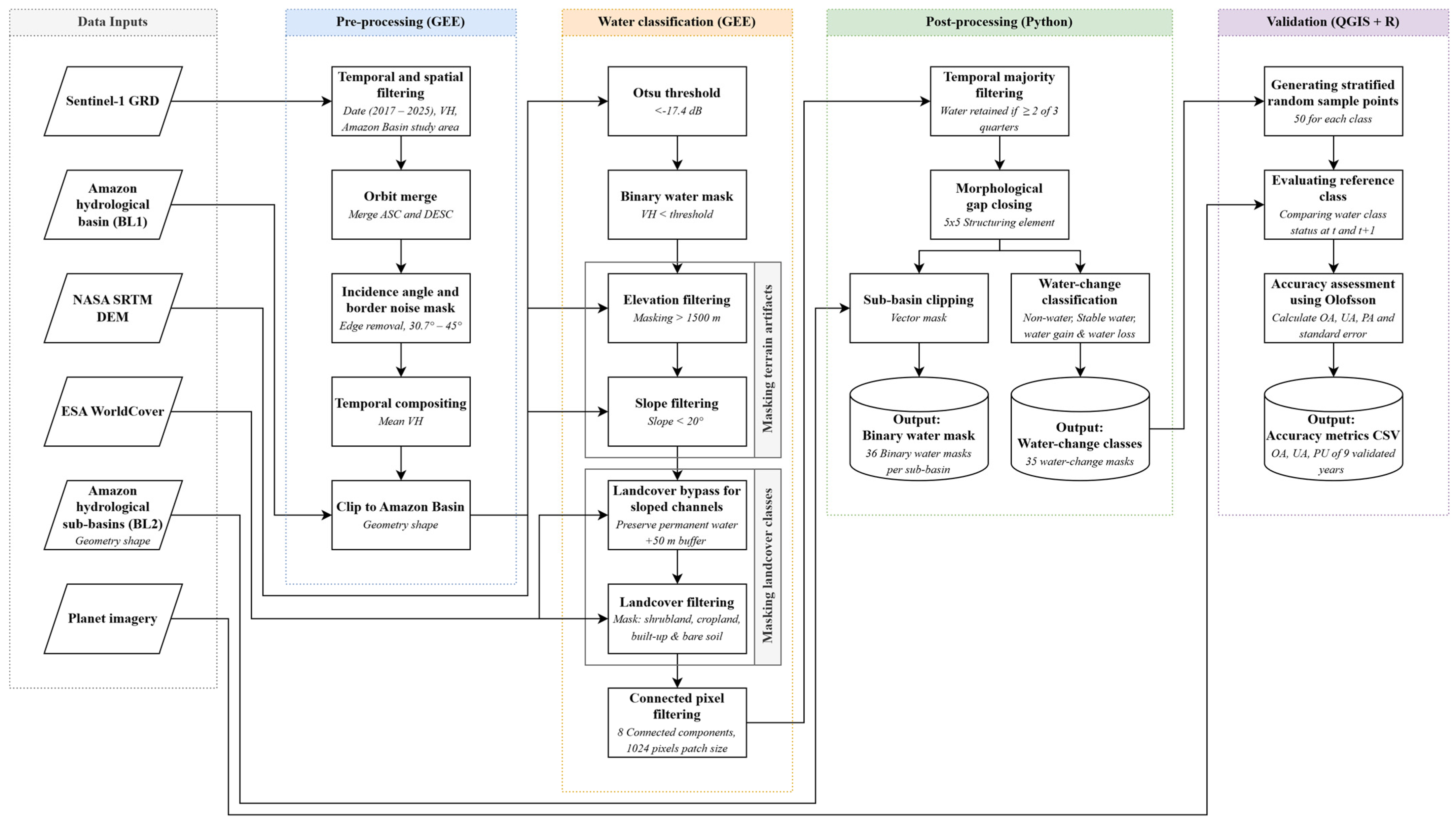
Surface water was extracted from the SAR imagery using a threshold-based classification approach, implemented in GEE (Figure 5).
Only VH polarization was used in this study due to smooth water surfaces strongly suppressing cross-polarized backscatter. This produces significantly lower backscatter values than the surrounding vegetation causing an inherently higher backscatter due to volume scattering (multiple reflections in vegetation and tree canopies), thereby yielding stronger land-water contrast [26]. In addition, VV polarization is more sensitive to Bragg-resonance caused by turbulent water surfaces such as wind- or rain-driven ripples or debris from surrounding vegetation, which is a common occurrence in the Amazon Basin [32].

2.3.2. Histogram Threshold-Based Water Classification

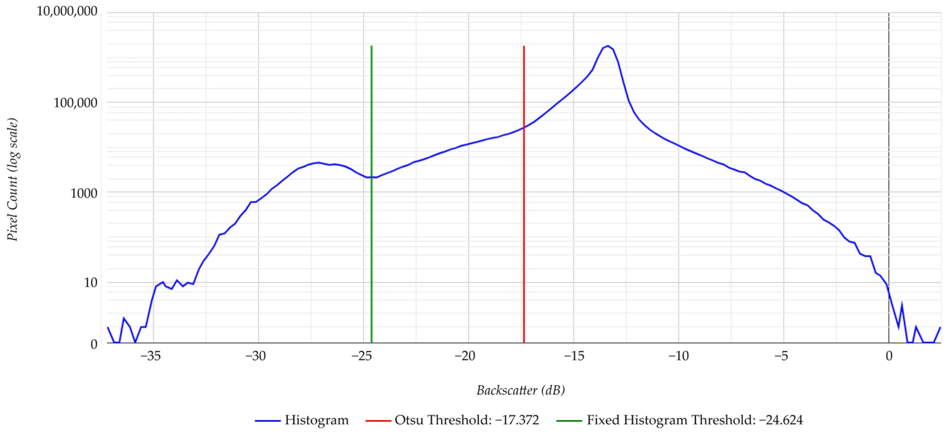
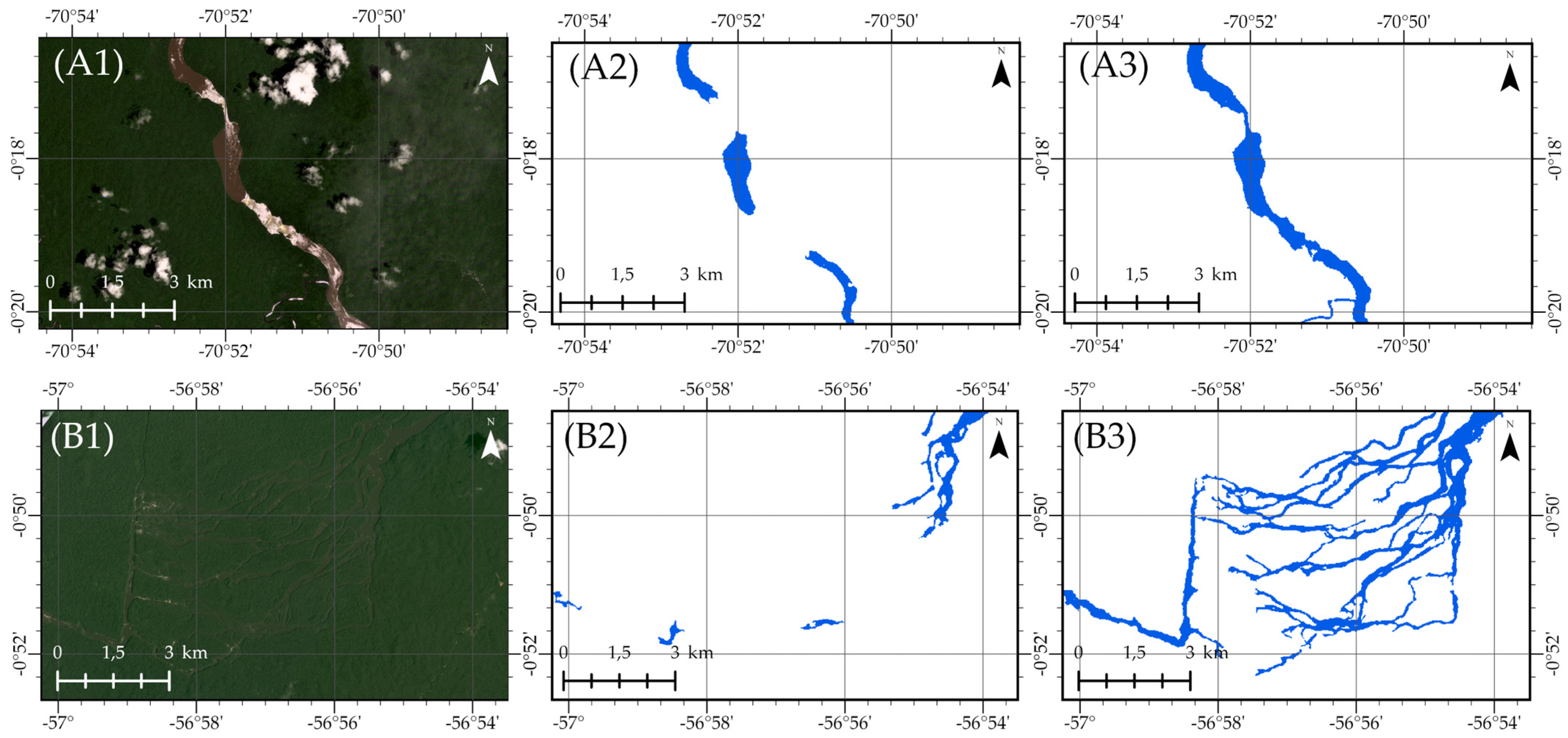
The water classification was based on dB backscatter intensity thresholding. Two approaches were assessed, firstly a histogram-based thresholding and secondly Otsu thresholding. Histogram thresholding applies to a thresholding value derived from the distribution of backscatter values manually sampled in 100 random locations of waterbodies, making sure to represent upstream- and downstream channels, (oxbow) lakes and floodplains; thereby resulting in a backscatter value threshold of −24.6 dB (Figure 6). The threshold-based method correctly classified river channels with relatively low commission error, but exhibited substantial omission errors. As a result, important channel sections were missing, preventing complete centerline extraction and limiting its suitability for monitoring geomorphological river dynamics. That is why Otsu thresholding was preferred in this study.

2.3.3. Otsu Thresholding

Otsu thresholding as proposed by Nobuyuki Otsu [57] determines the optimal threshold by maximizing the between-class variance in a bimodal histogram. Otsu’s formula to generate the threshold value is formulated as follows:
σb2 (t) = ω1(t)ω2(t) [μ1(t) − μ2(t)]2
where ω1, ω2 are class probabilities and μ1, μ2 are class means. After computing the Otsu threshold using the SAR data histogram, a threshold value of −17.4 dB was retrieved (Figure 6). Although Otsu thresholding assumes a bimodal distribution of the histogram [31], which is not the case for the unimodal histogram of the Amazon, it provided a more inclusive classification of waterbodies than the histogram method, as seen in Figure 7A,B. By better preserving these finer scale features through Otsu thresholding, river morphodynamics could be analyzed better in a later stage. This leads to the water classification threshold to be formulated as follows:
dB ≤ −17.4 = water
dB ≥ −17.4 = non-water

2.3.4. Terrain- and Landcover-Based Filtering

However, this more permissive threshold also introduced more false positives. The added commission error caused by choosing Otsu over the histogram method was reduced by introducing several filtering steps to the water mask, including elevation-, slope- and landcover filtering.
Firstly, terrain artifacts were masked out, a SRTM DEM-based elevation mask was used to exclude areas above 1500 m. This cutoff value resulted in the highest elevation parts of the Andes being filtered out without removing low laying mainstem rivers. Additionally, for the areas of the Andes below this cutoff threshold a slope filter was applied, keeping only areas with slopes below 20°. These filters reduced misclassifications in mountainous terrain where layover and shadow effects were most apparent. However, because some rivers rapidly descend in the Andes, sections with slopes greater than 20° were unintentionally also filtered out, causing gaps in the water mask. To address this limitation, a reverse water filter was applied to preserve these steep rivers. The slope filter was combined with a rule-based exception using the ESA WorldCover dataset. This filter allowed for SAR-derived water mask pixels to bypass the slope filter when they spatially overlap with the permanent waterbodies class from the landcover data. To reduce omission errors inherent in the landcover dataset the permanent waterbodies class was buffered by 50 m to preserve river morphology.
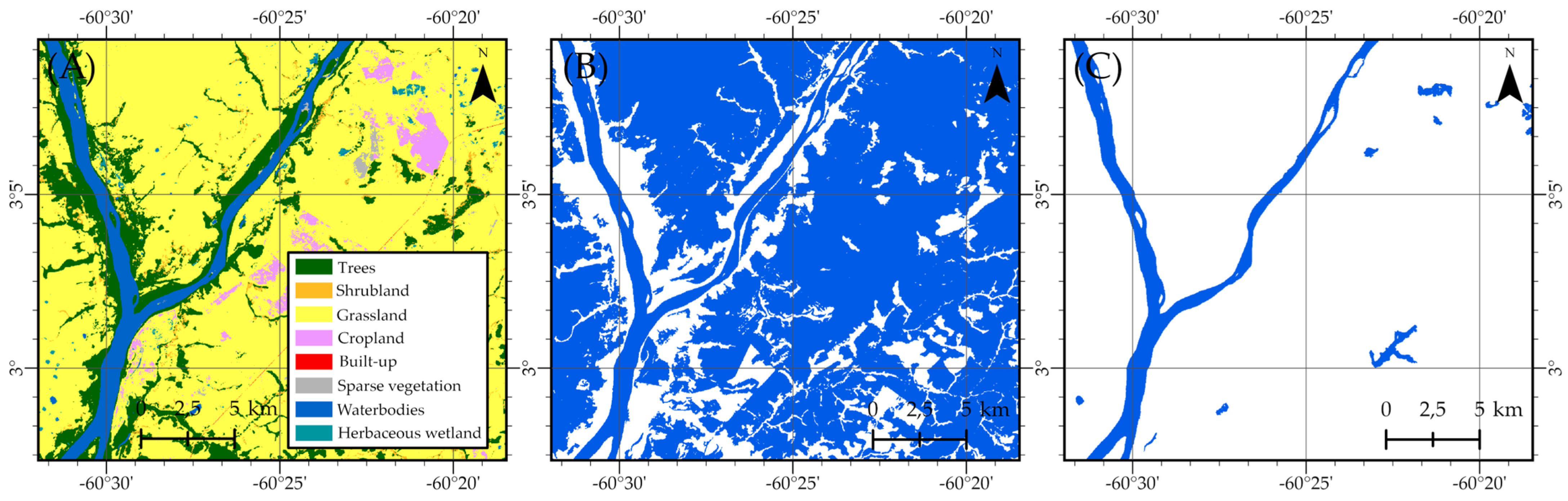
Secondly, additional landcover filtering was applied to the rest of the water mask to remove false positives. Pixels overlapping with shrubland, grassland, cropland, built-up areas and sparsely vegetated surfaces were excluded from the water mask, thereby removing areas prone to low backscatter values (Figure 8). Finally, a connectivity filter with a patch size of 1024 was applied to remove classification noise and only keep hydrologically meaningful features. This ensures that only larger continuous waterbodies such as rivers and (oxbow) lakes were preserved.

2.4. Post-Processing

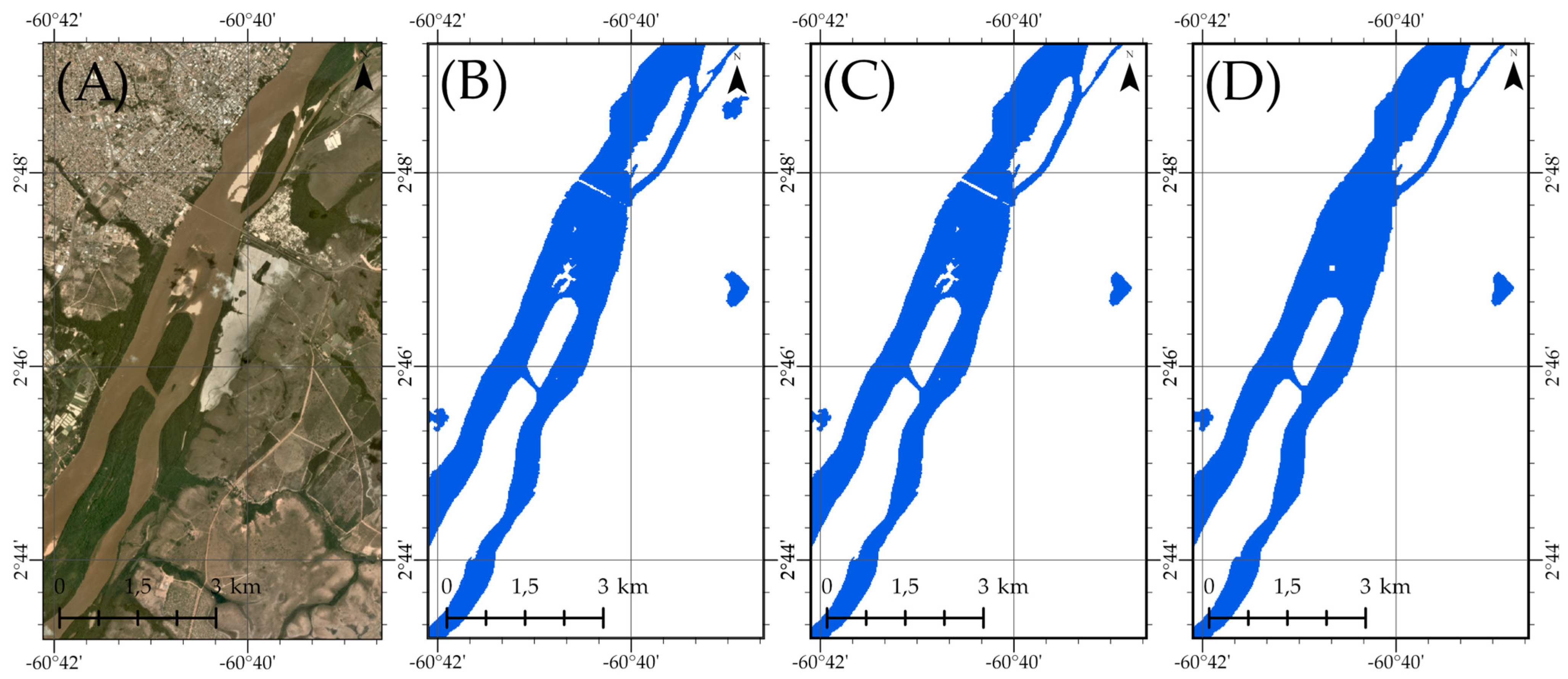
After all binary water mask images were exported (Figure 9A; imagery reference and 9B; raw data), two more post-processing steps were made to prepare the data for planform river metric extraction, using empirically selected filter parameters. Firstly, a temporal majority filter was applied to further reduce remaining classification noise not picked up by the connected component filter and to improve temporal consistency. This post-processing step makes sure that short-term misclassifications caused by seasonal effects such as crops being watered, rainfall or droughts, were suppressed. This filter preserves the channel structures and minimally affects river morphology (Figure 9C). For each pixel in the datasets, a centered three-image temporal window was used. This consisted of the previous (t − 1), current (t) and subsequent (t + 1) quarters, where a pixel was classified as water if at least two out of three images shared water presence. This filter was expressed as follows:
W t ( x ) =   1     i f   W t 1 x + W t x + W t + 1 x 2 0     O t h e r w i s e
where Wt(x) represents the binary water classification of pixel x at time t. For the first and last images that do not have one image before and after, another stricter formula was used. The first and last timesteps were expressed as follows:
First timestep: Wt(x) = Wt(x) ∧ Wt+1(x)
Last timestep: Wt(x) = Wt−1(x) ∧ Wt(x)
After temporal filtering, a morphological gap-filling filter was applied to fill gaps in river networks. These gaps are primarily caused by misclassification errors or anthropogenic structures such as bridges and dams. These structures disrupt the radar signal, creating gaps in the binary water mask. To address this, a gap-filling filter using a binary closing operation was applied. This expands the water mask to fill gaps and connect nearby pixels, then it contracts again to restore the original river channel shape, while maintaining the filled gaps (Figure 9D).
A square structuring element or kernel was used as the filling window. We evaluated three kernel sizes (3 × 3, 5 × 5 and 7 × 7). The 3 × 3 kernel was too small to compensate for larger gaps caused by wider dams, while the 7 × 7 kernel introduced additional blocky artifacts. Therefore, we selected the 5 × 5 kernel as the optimal balance. It effectively restored connectivity between narrow and moderate gaps while still maintaining the majority of the original river channel shapes.

2.5. Water-Change Validation

To assess the capability of the derived water masks in capturing geomorphological river dynamics, multi-class water-change maps were created using the binary water masks. This was calculated by using a pairwise comparison between a single water mask and its subsequent timestep (t and t + 1). For each pixel in the dataset, a change class was assigned based on its state between the timesteps. This created four water-change classes: non-water (t = non-water, t + 1 = non-water), stable water (t = water, t + 1 = water), water gain (t = non-water, t + 1 = water) and water loss (t = water, t + 1 = non-water).
Validation was conducted by visually assessing high spatial resolution optical PlanetScope data. We selected a total of 18 Planet (three monthly) composite reference images. The images were chosen based on minimal cloud cover, while ensuring the representation of all four quarters across all studied years. This approach provided reliable reference data while minimizing the influence of cloud cover that could hinder accurate validation. Each pair of Planet images represented a timestep of t and t + 1, matching the water-change validation maps created during pre-processing, resulting in a total of nine validated water-change masks.
The validation followed a stratified random sampling design based on each of the four water-change classes: non-water (i), stable water (ii), water gain (iii) and water loss (iv). For each class, a total of 50 points were randomly generated in the defined polygons, without any spatial clustering constraints or forced placement parameters. Fifty sample points were selected to balance statistical reliability with the practical constraints of manual and visual interpretation across different image pairs [19]. This was repeated for nine different water-change maps resulting in a total of 1800 sample points. This was deemed a sufficient sample size for manual validation between different timesteps and four change classes, while still being able to produce stable class-wise accuracy estimates.
Each point was manually assessed using Planet imagery at timesteps t and t + 1 as reference data. Water presence was evaluated at both timesteps and assigned a reference class according to the observed transition: non-water, stable water, water gain or water loss.
Accuracy assessment was performed in R (version 4.4.2) using the area-weighted validation approach as proposed by Olofsson et al. [58], implemented via the mapaccuracy package. A key component of this method is the use of strata weights, computed from the mapped area proportions of each change class to represent the total mapped area of each class, using the terra package (Appendix B). These weights correct for unequal sampling probabilities across class proportions that are imbalanced. The calculated validation metrics include Overall Accuracy (OA), Users Accuracy (UA), Producers Accuracy (PA) and standard errors at 95% confidence interval derived as 1.96 x SE. Because Olofsson’s method calculates validation metrics for each change map individually, an area-weighted pooled estimate was also calculated to summarize overall accuracy across the entire time series [59], where each period’s accuracy is multiplied by the fraction of total mapped area over all datasets. Therefore, weighing each period’s contribution by its mapped area is consistent with the area-proportional estimation approach as proposed by Pickens et al. [60]. This method results in differences in spatial extent and class distributions between timesteps being accounted for.

2.6. Planform River Metric Extraction

2.6.1. River Planform Metric Selection

For the extraction of planform river metrics, a subset of widely used metrics was selected based on the literature review (Appendix A). For this study, the three most used metrics in literature that are derivable from SAR-based binary water masks were chosen, these being:
  • Migration rate
  • Sinuosity
  • Mean channel width
These selected metrics were deemed suitable for large-scale analysis of river planforms and describing their geomorphological change over time. With the addition of the water-change maps used for validation, stable water, water gain and water loss can also be extracted. These selected metrics combine the description of geomorphological change in channel planforms with indicators of lateral mobility and water extent.

2.6.2. Data Preparation

All data was reprojected to ensure that all metric calculations are geometrically the same across the full longitude and latitude of the study area. The projection EPSG: 6933 was used to preserve the shape of the large Amazon Basin across multiple UTM zones.

2.6.3. Skeletonization and Graph Construction

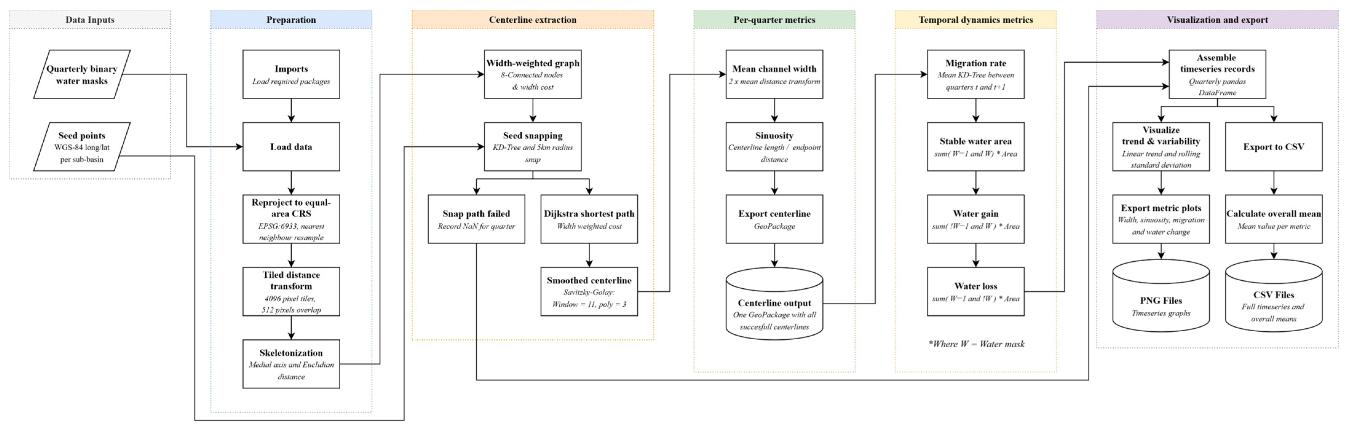
Different algorithms already exist to calculate river metrics, such as RivMap [61], RivWidth [62], RivaMap [22] and SCREAM [19]. These are well-received options, each with slightly different approaches on calculating river metrics. But all methods have in common that river centerlines (a single line element following the exact center of a river) are necessary to calculate said metrics. In this study, channel centerlines were extracted using a width-weighted shortest path algorithm using Python (version 3.13) (Figure 10).
First, the binary water masks were skeletonized using medial-axis and a tiled Euclidean distance transform [63]. Then, a graph was computed where each skeleton pixel forms a node and eight-connected neighbors form the edges [64,65]. Instead of centerlines being generated through the shortest possible path, an edge cost formula was used to assign traversal cost to every edge in the skeleton graph. This ensures that centerline routes go through the widest available channel, thereby allowing for the calculation of metrics in the mainstem and not a side-channel where the assumption was made that the mainstem of a river is the widest available channel. This edge cost was defined as follows:
C i j   =   d i j 1 w i j α
where Cij is the cost of moving between nodes i and j, dij is the step length between neighboring pixels, wij is the mean channel width between nodes i and j, and α is the weight controlling how strong width influences the cost, which is set to 2.

2.6.4. Centerline Extraction and Smoothing

To generate the centerlines, several approaches were tested including Principal Component Analysis (PCA) and cumulative-width scoring [66]. While these did automatically derive channel centerlines, they could not independently infer which path is the mainstem of a sub-basin. Therefore, if a tributary channel was long or wide enough these purely algorithmic approaches would occasionally choose the tributary path instead of the mainstem causing misleading metrics. Instead, a Dijkstra’s algorithm was applied to generate centerlines between manually defined upstream and downstream seed points per sub-basin [67,68]. These seed points were selected by deriving latitude and longitude coordinates of the start- and endpoint of the river mainstem. In the case that there was no skeleton node at the specified location, the seed point snapped to the nearest skeleton node within a 5-km search radius.
All of the generated centerlines were then smoothed using a Savitzky−Golay filter [69]. For this filter, a smoothing window of 11 was used and a smoothing polyorder of 3. This reduced blocky “zigzag” patterns, which are caused by calculating the centerline from binary rasters and preserved smooth river morphology.

2.6.5. Metric Calculation

After centerline extraction, the six chosen metrics were derived per quarter. Mean channel width was computed as twice the distance-transform radius across all water pixels. Width was then calculated as the arithmetic mean of all node-wise width samples along the extracted centerline for a given quarter, providing a reach-averaged estimate of channel width [62,70]. Sinuosity was defined as the ratio of centerline length to the straight-line distance between start and end points [71,72]. Migration rate was calculated as the symmetric mean nearest-neighbor distance between subsequent quarter centerlines, using KD-tree [73,74,75]. Stable water, water gain and water loss were derived by bitwise comparison of subsequent binary water masks, where each quarter was multiplied by the pixel area in square meters. For an overview containing all parameters used in the entire methodology, see Appendix C.

3. Results

3.1. Water Masks and Validation

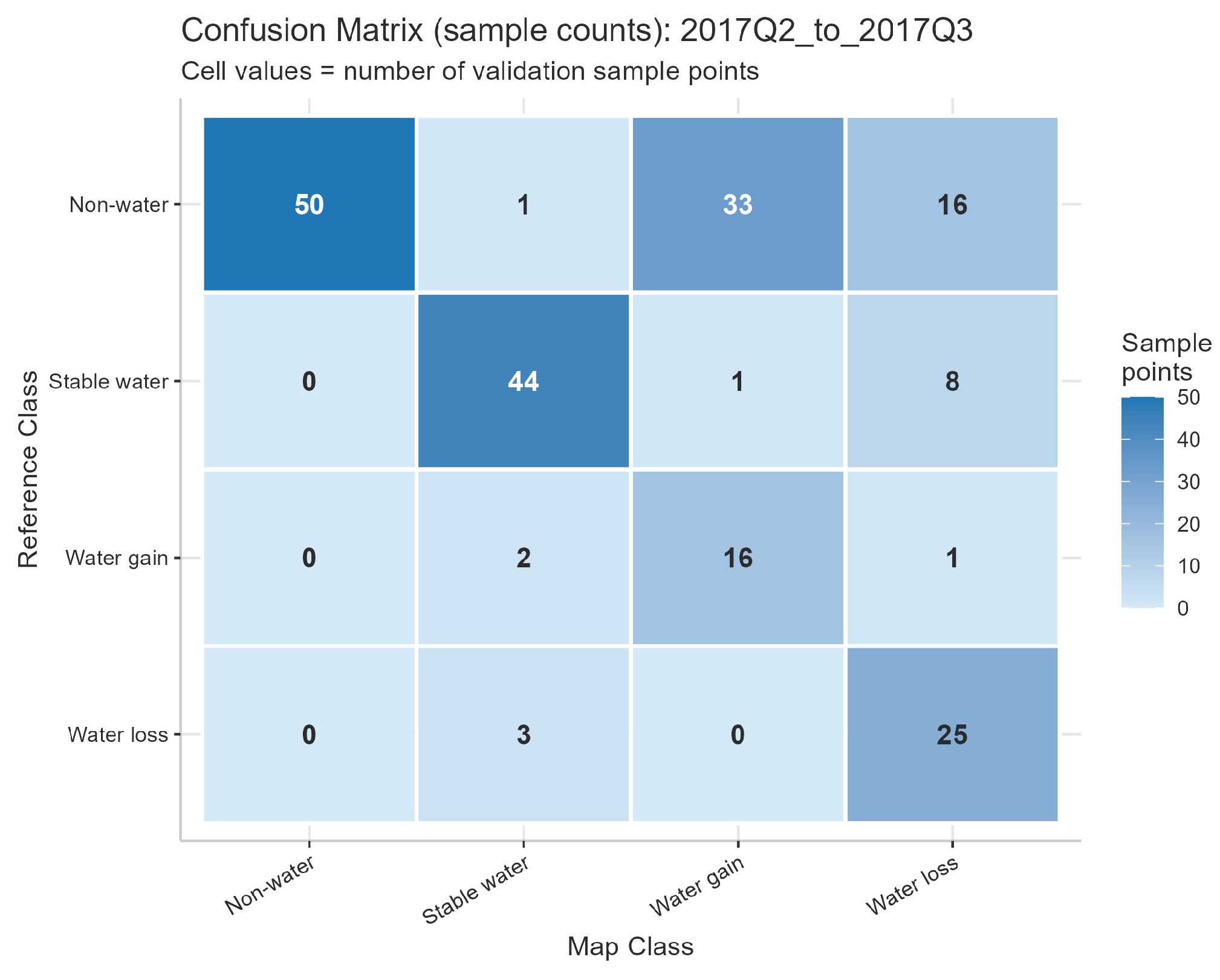
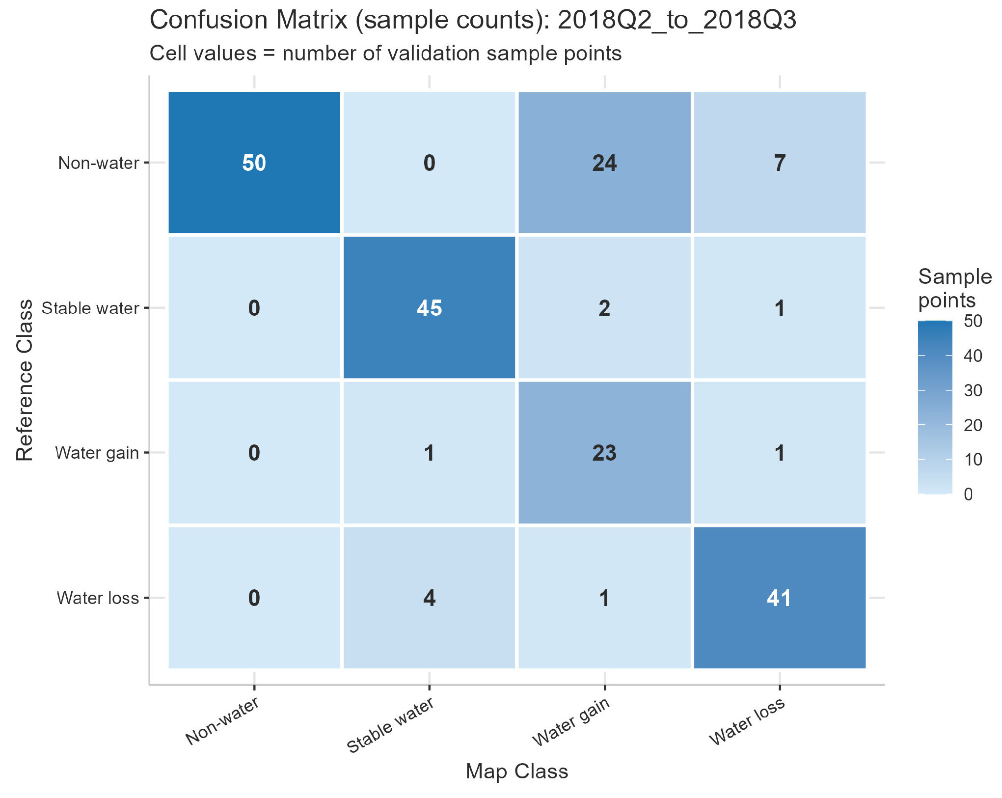
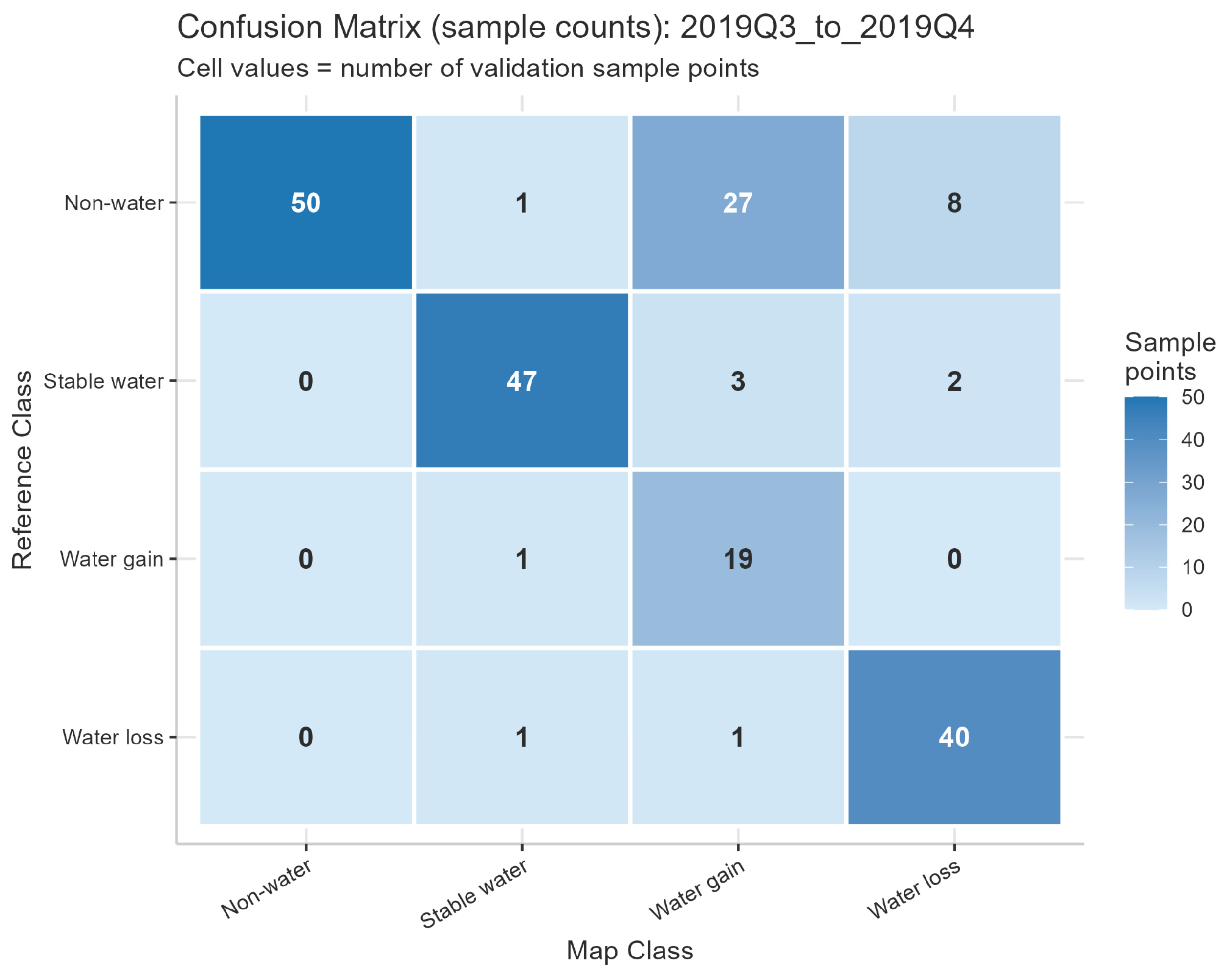
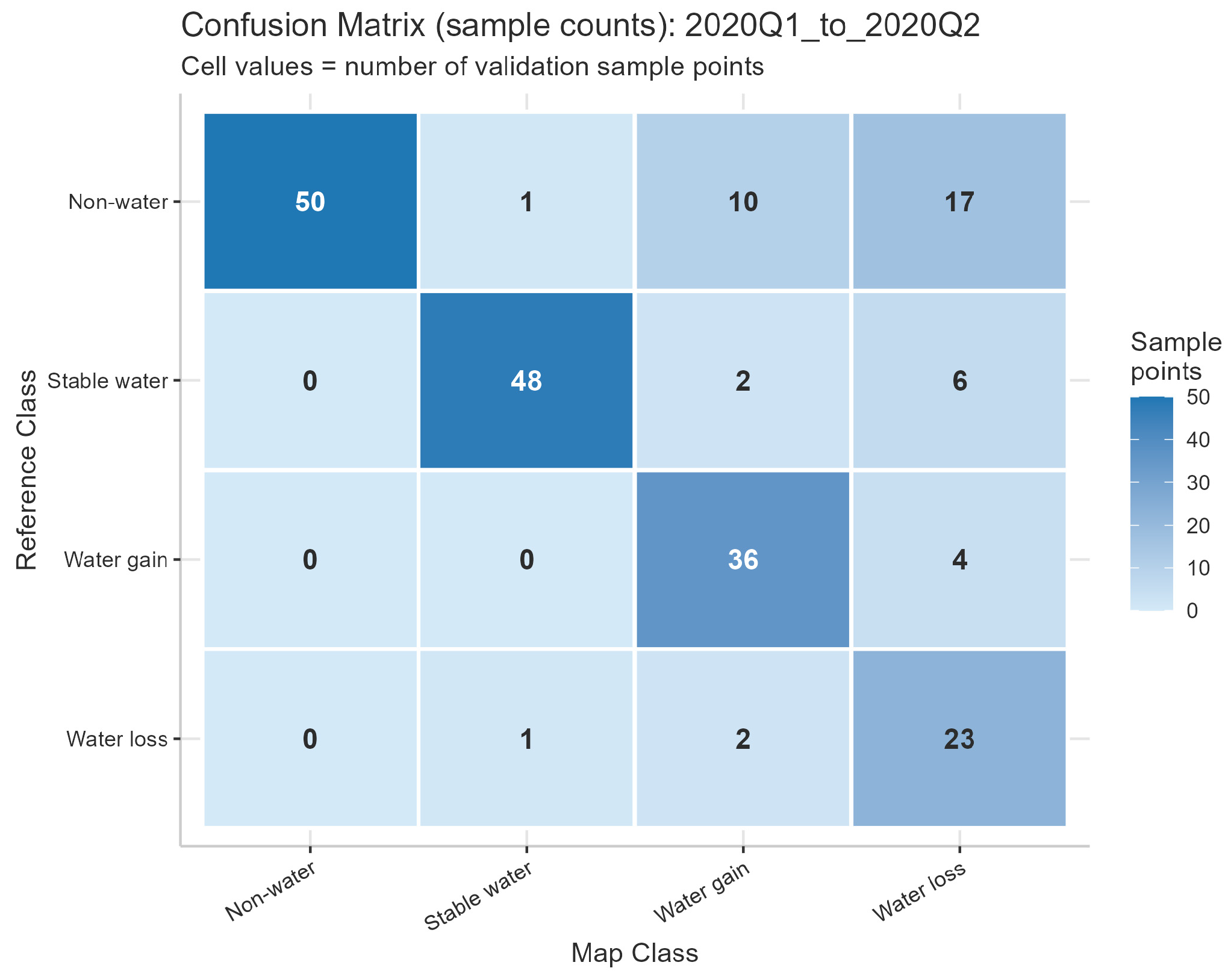
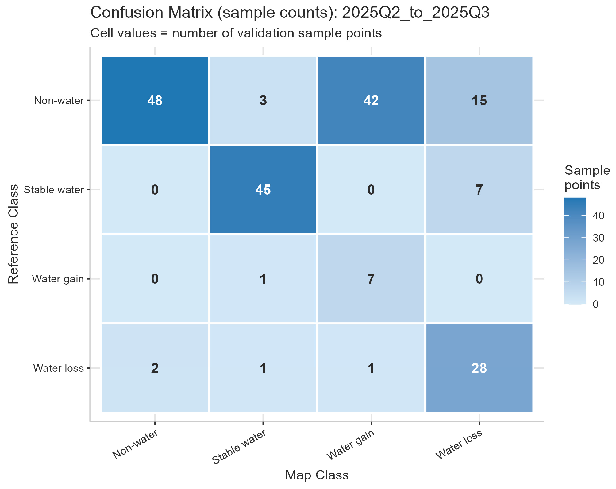
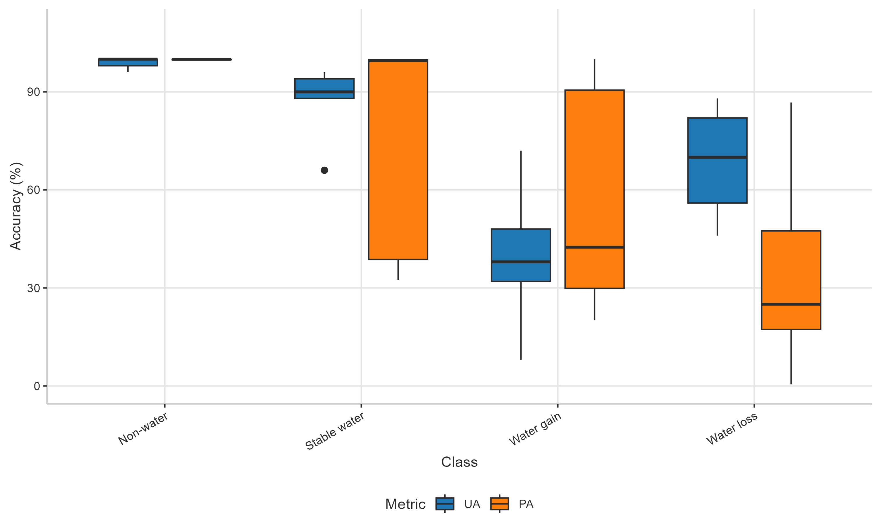
The final dataset consists of 36 quarterly binary water masks covering the full Amazon Basin, spanning from 2017 to 2025 with an overall accuracy of 98.48%. It should however be noted that this OA is dominated by the non-water class which consists of a substantially larger area than the other classes. As a result, the OA is effectively driven by non-water classification performance. The class-wise accuracy assessment showed the highest UA (99%) and PA (99.8%) for the non-water class (Figure 11). The stable water class indicated high UA values (90%) with lower PA values (78.3%).
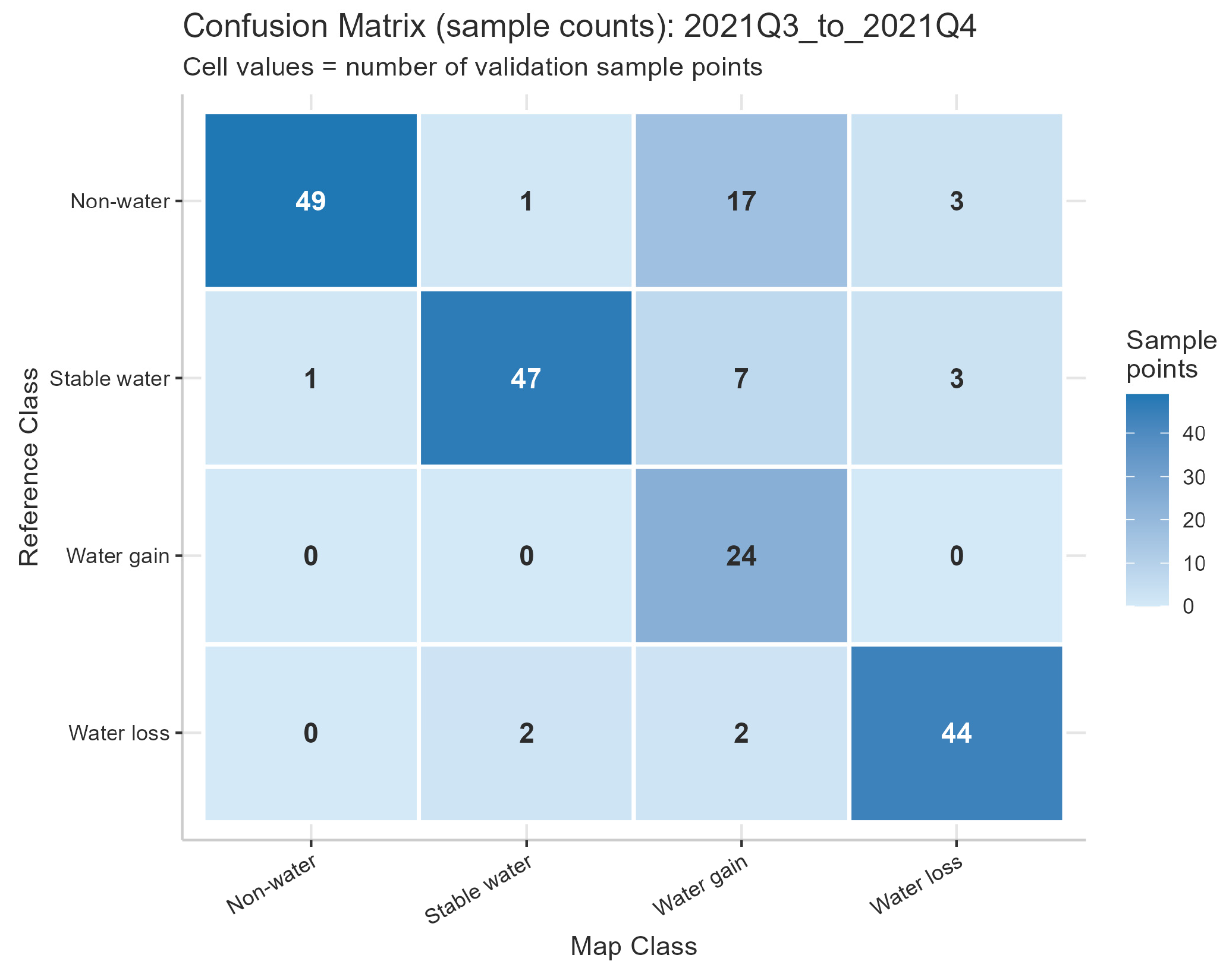
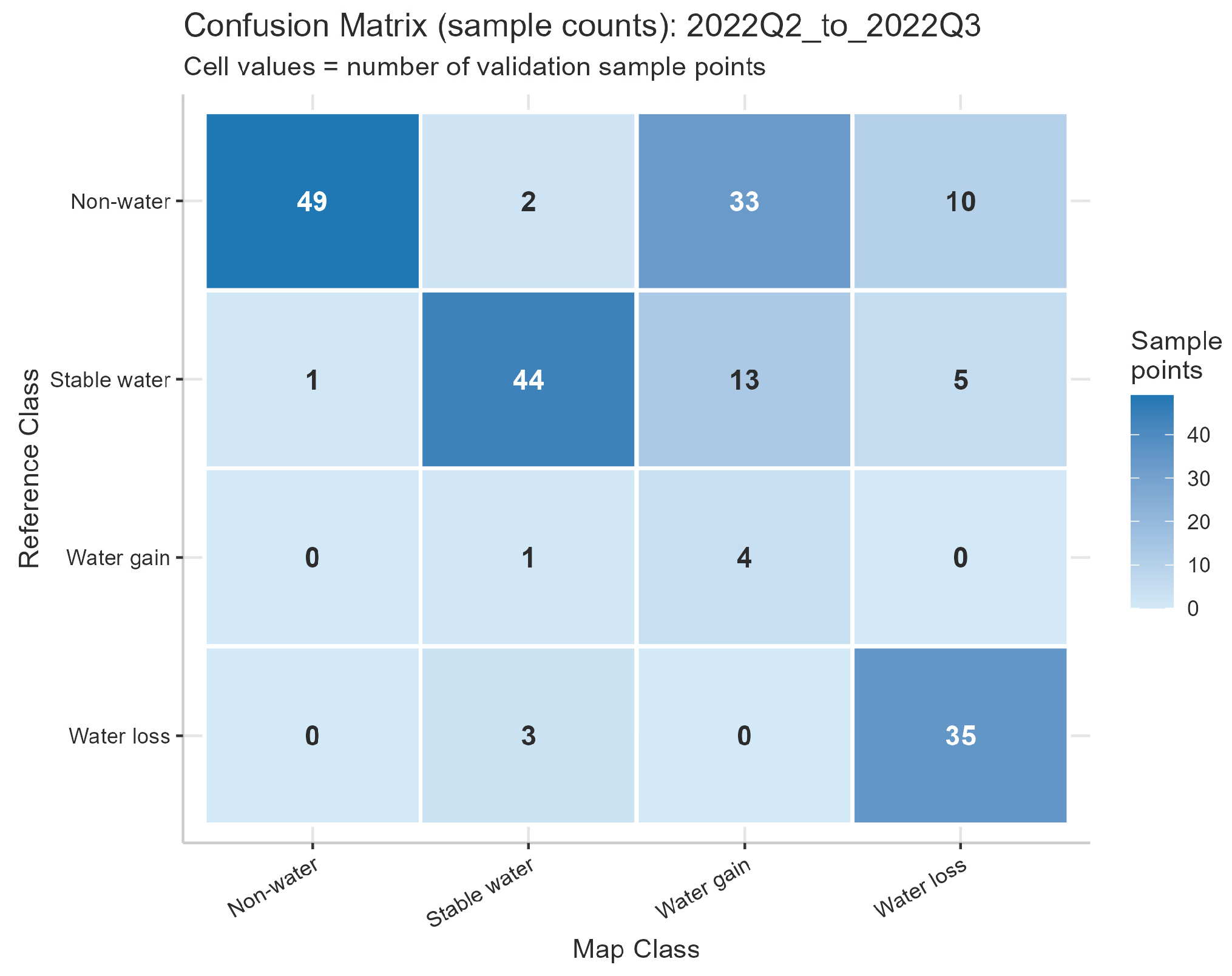
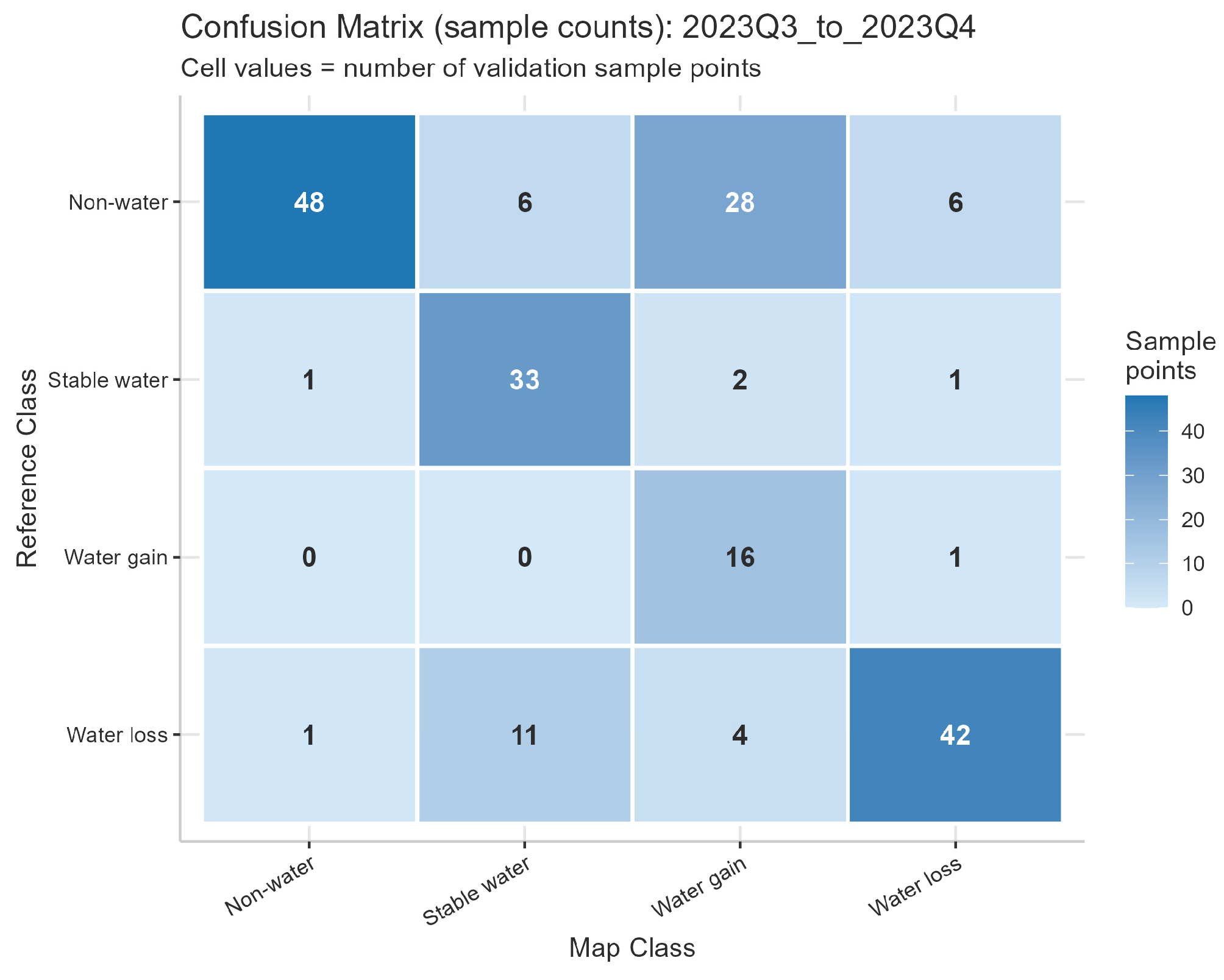
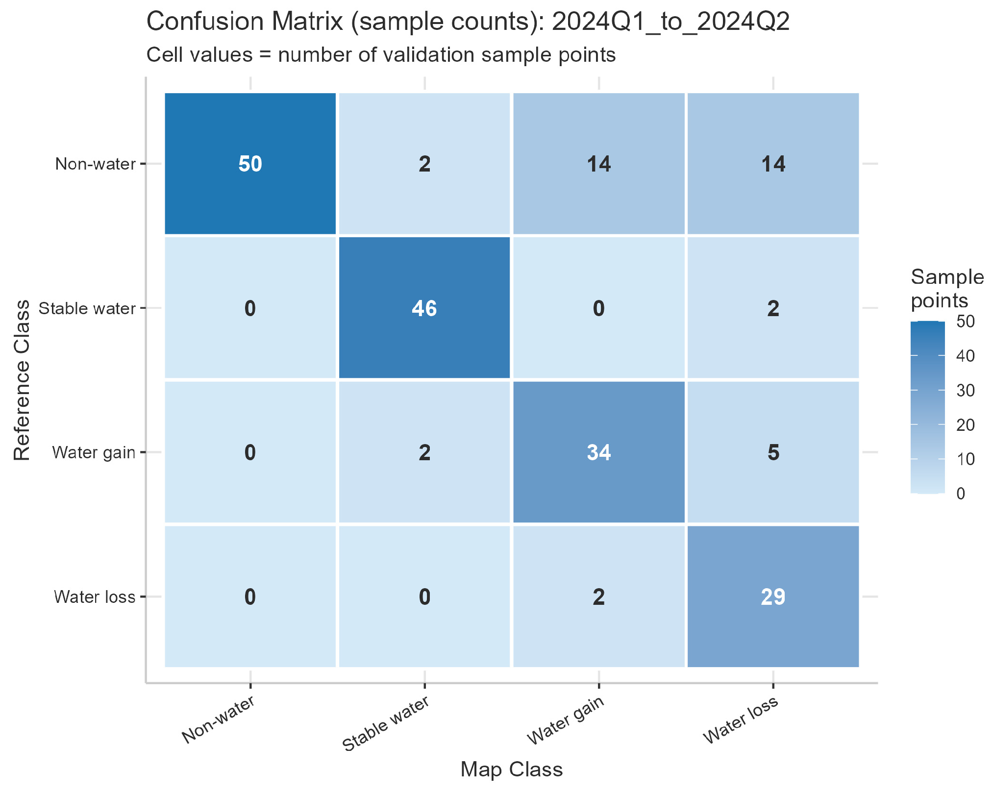
Lower accuracies are observed for the water gain and water loss classes. Water loss has a higher UA (70%) than water gain (38%), while both classes show a low PA value (42.45% for water gain and 25.03% for water loss). A full overview of all confusion matrices and per quarter UA and PA values is attached in Appendix D. The high reliability of the non-water and stable water classes ensures a consistent representation of stable river geometry, which is the primary requirement for centerline extraction and metric calculation. The lower accuracies in water gain and water loss have a limited impact on the generation of these metrics.

3.2. Planform River Metrics

3.2.1. Main Channel Centerline Generation

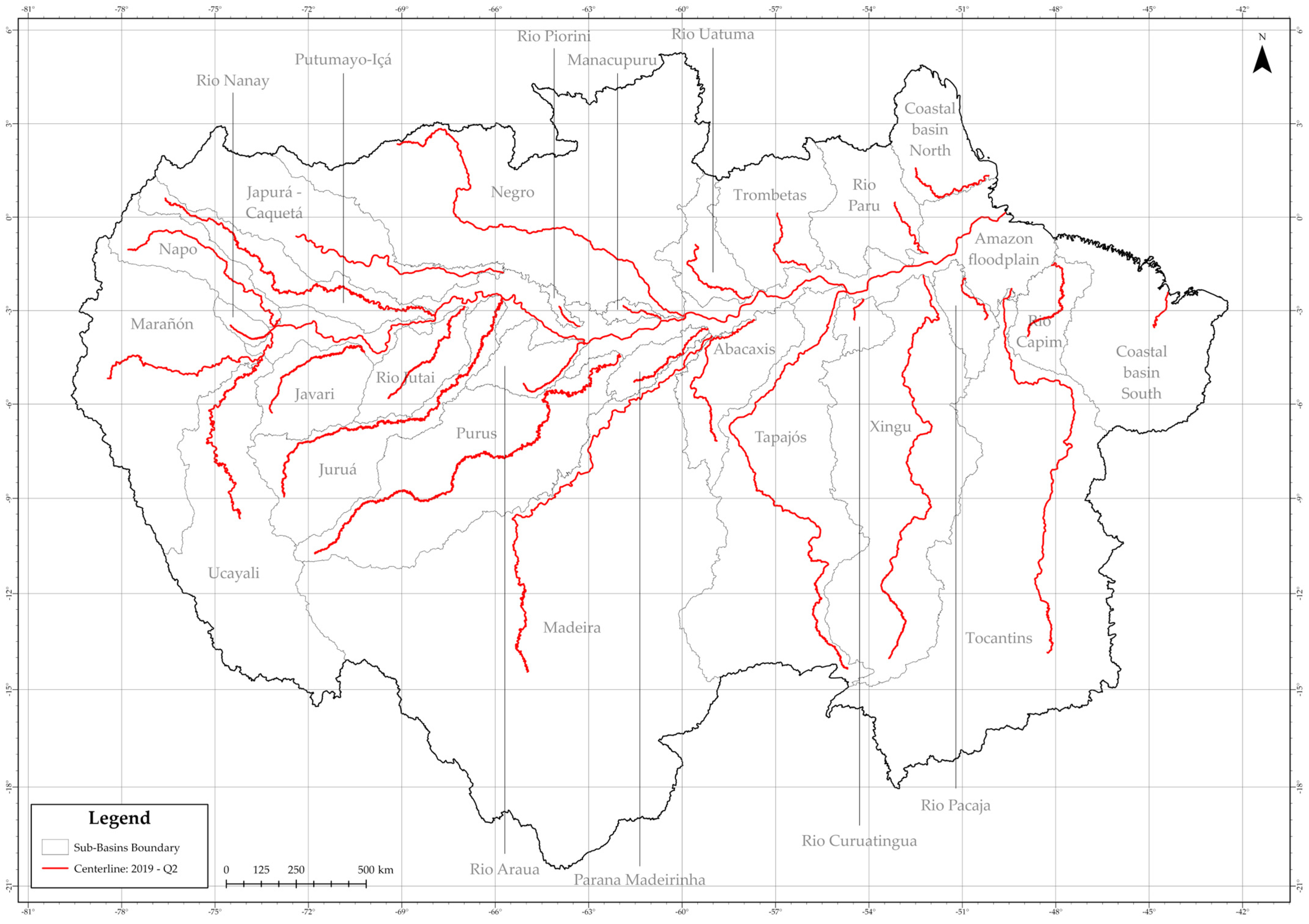
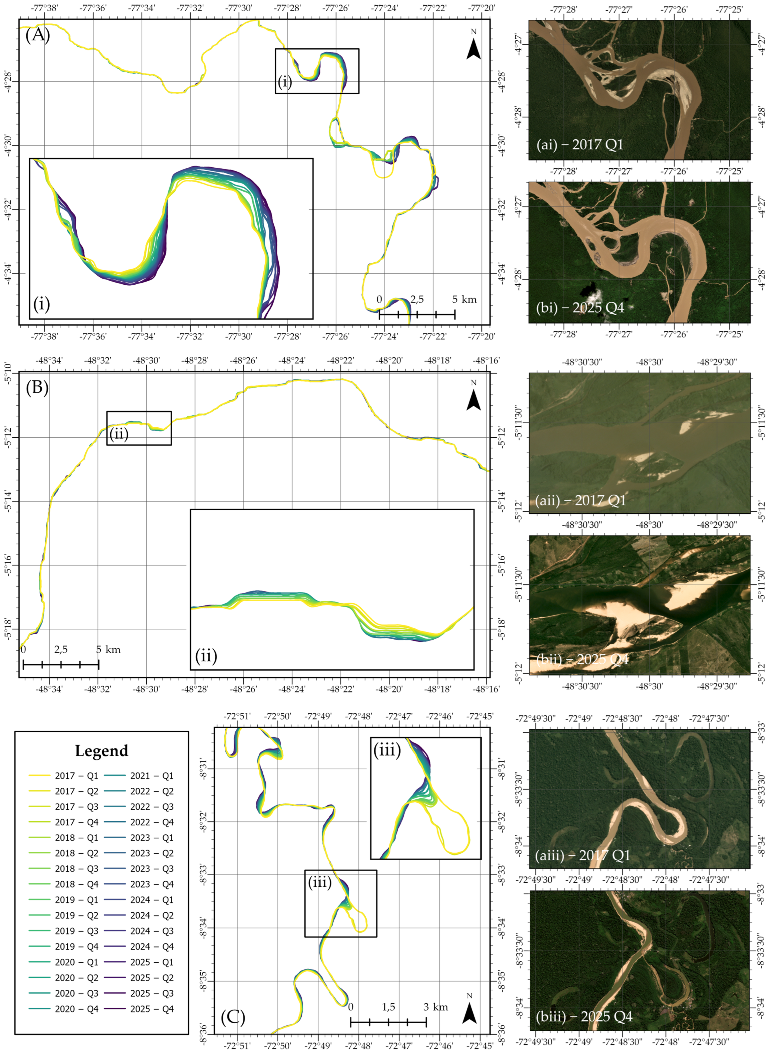
The extracted centerlines for all sub-basins as shown in Figure 12 provide an overview of the spatial extent of the derived main channel paths across the Amazon Basin. The results show that centerlines were successfully generated for most of the quarters. Although occasional gaps occur in the water mask, the overall generation of centerline paths remains stable.

3.2.2. Per Quarter Centerline Generation

Different centerlines were extracted throughout the years and sub-basins. The centerlines follow the central direction and structure of the river channels consistently across all quarters. Especially differences in migration rate and sinuosity between upper, middle and lower Amazon become apparent (Figure 13A–C).

3.2.3. Sub-Basin Mean Metrics

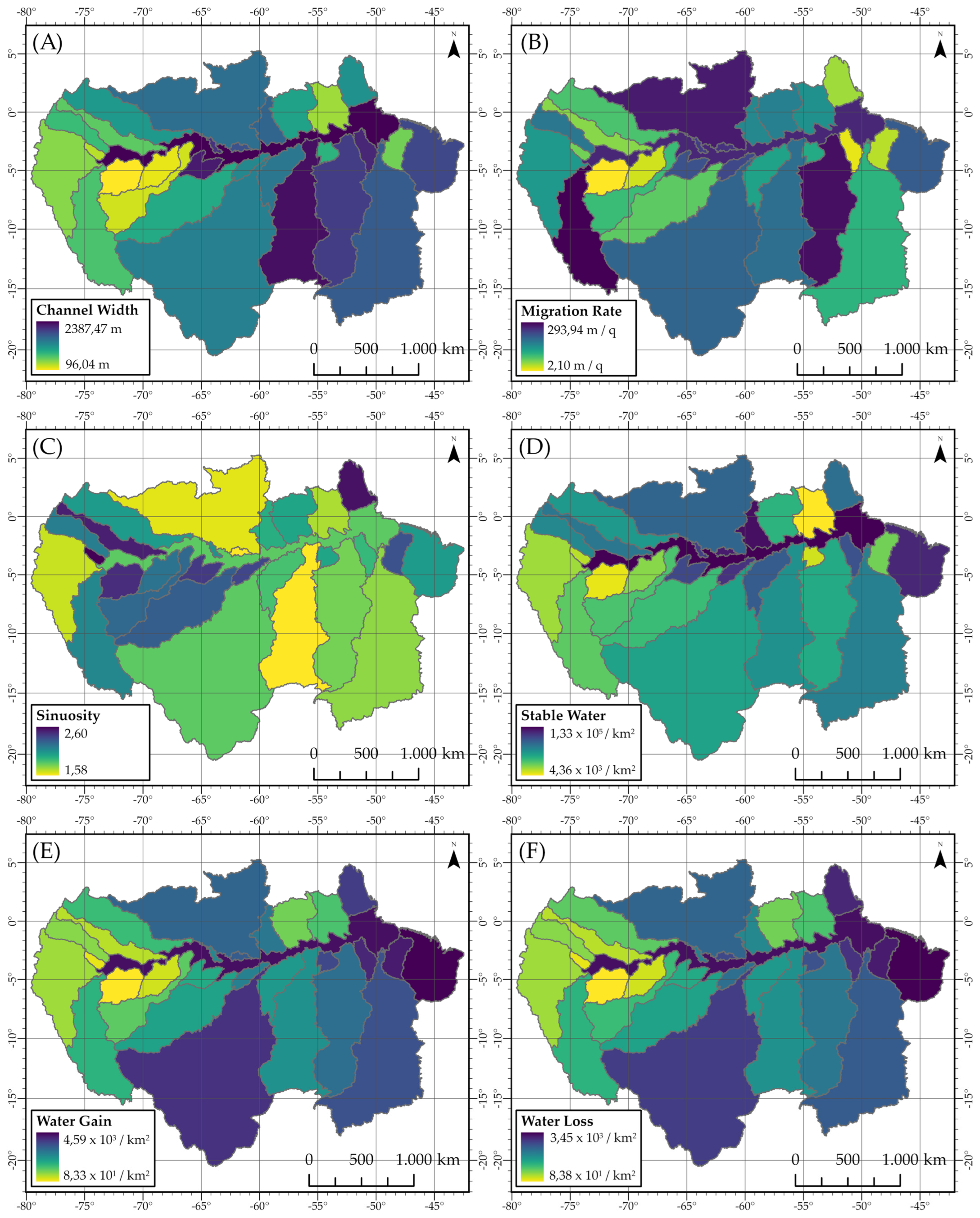
The mean of the six river metrics (mean channel width, sinuosity, migration rate, stable water, water gain and water loss) show the spatial variability in river morphology changes and how they differ per sub-basin across the entire Amazon Basin (Figure 14).
Mean channel width ranges from 96.04 m to 2387.47 m, with the Amazon floodplain recording the widest channel (2387.47 m), followed by larger tributary systems such as the Tapajos (1978.84 m) and Rio Araua (1786.97 m). The narrowest channels occur in the smaller sub-basins such as the Javari (96.04 m) and Rio Jutai (138.67 m), suggesting that mean channel width scales with sub-basin surface area extent.
Migration rates are the most spatially heterogeneous metric, ranging from 2.10 to 293.94 m/q, with no clear up- or downstream gradient. The upper Ucayali stands out with the highest rate (293.94 m/q), with the second highest Xingu basin having a much lower migration rate (96.81 m/q). The Amazon floodplain itself records a moderate 67.02 m/q despite its size, showing consistency with its anastomosing and low-lateral mobility character [4]. Several upstream basins such as the Javari (2.34 m/q) and Rio Jutai (2.29 m/q) show very little migration. But lower laying sub-basins such as the Rio Pacaja (2.10 m/q) and Rio Capim (3.17 m/q) also show very little migration rate, indicating that the position in the upper or lower stream of the Amazon Basin has less effect on the migration rate.
Sinuosity ranges from 1.42 to 2.67, where a low sinuosity signifies a relatively straight river channel and a high sinuosity a larger degree of meandering [6]. This metric shows clear spatial patterns, distinguishing anastomosing from meandering river planforms. The anastomosing Amazon floodplain (1.52), Madeira (1.52) and Negro (1.71) all record low sinuosity, showing their multi-thread planform [4,14]. While the Purus (2.67), Javari (2.64) and Jurua (2.58) reach high sinuosity values, consistent with their active meandering pattern in low-gradient alluvial environments [12].
The stable water-change metric is dominated by the Amazon floodplain sub-basin, which records the highest stable water of 132,599.61/km2, thereby indicating that this body of water is consistently inundated by the large amplitude of tributary basins discharging water into the mainstem. Water gain and water loss however are highest in the Coastal basin south with water gain at 4593.54/km2 and water loss at 3451.71/km2. Large basins such as the Negro (19,734.95/km2) and Madeira (12,412.64/km2) also show high stable water metrics, while smaller tributaries such as the Javari (85.30/km2) and Rio Nanay (99.68/km2) record very low values across all three metrics. The spatial patterns of water gain and water loss are similar across sub-basins, most likely due to seasonal flood cycles [1,3,7].
The sub-basin comparisons presented here are descriptive in nature. Statistical significance of differences in mean channel width, sinuosity, or migration rate between sub-basins was not formally tested, as the time series for each metric constitute a single continuous observation record per basin rather than independent repeated timesteps. Instead, this study produced quantitative metrics through time series and mean metrics. All time series data for each sub-basin is attached in Supplement S3, and a more detailed description of all metric values per sub-basin is attached in Appendix E.

3.2.4. Temporal Patterns

Several notable temporal patterns emerge at the basin-wide level when analyzing the time series in Supplement S3. Sinuosity shows generally stable trends across most sub-basins, consistent with the pattern typically associated with planform transformation. Migration rate, on the other hand, is variable from quarter-to-quarter and does not show consistent directional trends, reflecting its sensitivity to individual flood pulses rather than gradual geomorphological change. The most pronounced signal is observed in the water-change metrics during the 2023 El Niño event, when the stable water area in the Amazon floodplain reached its minimum recorded value across the entire time series.

4. Discussion

4.1. Large-Scale Extraction of Planform River Metrics Using SAR-Based Data

This study aimed to address the applicability of SAR-based water masks for extracting river planform metrics at a large, basin-wide, spatial scale. The results indicate that SAR-derived water masks can be used to generate geomorphological river metrics, including migration rate, mean channel width, sinuosity and water surface area dynamics, across the Amazon Basin. The main contribution of this study is the development of a scalable, basin-wide framework for monitoring river morphodynamics using SAR-based data. Rather than providing direct validation of the derived geomorphological metrics themselves, the study shows that SAR-based water mask time series can support a consistent, large-scale assessment of river-channel change.
A key advantage of the approach is its independence from atmospheric conditions. Unlike optical sensors, SAR enables repeated observation regardless of cloud cover or daylight, which is critical in the persistently cloudy Amazon Basin [26]. This makes SAR well suited for temporally consistent image series and for monitoring seasonal as well as interannual river change.
These findings are in line with observations by Marchetti et al. [29], who noted that small-scale morphological changes in river channels are often difficult to detect with SAR because of spatial resolution constraints. Their study suggested that SAR may be more suitable for broader-scale geomorphological patterns than fine-scale channel adjustments. The presented results support this interpretation: although minor changes may remain unresolved, larger-scale river dynamics and planform metrics can be extracted at basin scale. Thus, this study confirms the limitations identified by Marchetti et al. while demonstrating the value of SAR for systematic large-scale geomorphological analysis.
At sub-basin level, the derived metrics reveal clear spatial differences in Amazon river dynamics. Variation in mean channel width, sinuosity, and migration rate reflects the geomorphological diversity of the basin. Mapped water gain and water loss areas provide further insight into changes in channel position and floodplain interaction. These interpretations should remain cautious, however, because water-change classes were less accurate than non-water and stable-water classes [1,3,7].
It should, however, be noted that the derived metrics provide a simplified representation of complex river systems such as the Amazon Basin. As argued by Legleiter et al. [76], summary metrics such as mean channel width and sinuosity capture general aspects of channel geometry but do not fully represent the spatial complexity of river morphology or the smaller-scale processes that underlie planform change.
Compared to optical remote sensing approaches, the SAR-based framework as shown in this study offers advantages in temporal consistency under persistent cloud cover [25], at the cost of reduced accuracy at mixed edge pixels and seasonal noise in sparsely vegetated areas [31]. Optical methods might benefit from a longer historical archive, but this relies on lower resolution images than Sentinel-1 SAR data, causing more classification error in upstream areas with smaller channels [6]. Additionally, the applicability in the Amazon is constrained to cloud-free images that are hard to achieve during the wet season, right when alluvial geomorphological change is highest [3]. Machine- and deep learning methods for water body mapping have demonstrated higher classification accuracies than simple threshold-based methods [31,36]. But this requires greater computational cost and has reduced transferability to new regions due to the need for re-training [26]. The threshold-based approach used in this study prioritizes scalability across the entire Amazon Basin for nine years, accepting some reduction in classification accuracy as an acceptable trade-off.

4.2. Transferability and Future Applicability

The methodology developed in this study is flexible and transferable to other regions and river systems, including analysis of side-channels instead of main-channels. Because the SAR-based water mask extraction and filtering rely on globally available open-source datasets, only limited adjustment in parameter settings may be required. There is potential for the scripts to be adapted for a potential automated execution on a quarterly cadence as new Sentinel-1 scenes become available. A future improvement could involve scheduled GEE scripts that generate new water masks upon image availability, thereby improving the long-term monitoring of river metrics. The SAR-based approach is particularly relevant in regions where atmospheric conditions limit constant optical observations, such as the tropics.
However, the sensor characteristics strongly affect water detection quality. As noted by Maciel et al. [1], C-band SAR data, as used in this study, have limited canopy penetration and therefore cannot reliably distinguish between flooded and non-flooded forests. This constraints water mask extraction in areas like the Amazon Basin, where dense vegetation can obscure narrow channels and floodplains.
Current and future improvements in longer-wavelength SAR mission may help address this limitation. Freely available L-band data from missions such as NISAR (launched in 2025) and ROSE-L (planned for launch in 2028) are less affected by vegetation and could improve water surfaces detection in densely forested areas. Additionally, higher resolution-SAR missions such as TerraSAR-X or COSMO may help to capture smaller-scale morphological changes, as was suggested by Marchetti et al. [29].

4.3. Temporal Dynamics

The temporal scope of this study captures nine years of planform river metrics, while seasonal fluctuations and climate extremes are observed (such as the 2023 El Niño drought), with the Amazon floodplain reaching the lowest levels of stable water and the highest levels of water loss during this period (as seen in Supplement S3.2) [1]. However, these patterns should be monitored over a longer time period to improve statistical robustness. Given the relative short Sentinel-1 time series (began in 2017) compared with longer-running optical sensors, the current time series may be too short to capture long-term trends.
With changing climate conditions expected to shift [1,3,27,77], river geomorphological processes are also likely to shift in the near future, making continuous monitoring essential. Especially as human populations continue to urbanize, water scarcity also increases [34], creating growing challenges for the management of water resources for consumption, sanitation and agriculture [27].
In the Amazon Basin, riverine communities depend on the rivers’ natural cycle for fishery, agriculture and navigation [13]. If extreme events continue to increase in frequency and intensity, these communities may face greater challenges, including mass fish deaths, disrupted transportation and crop failure [1,3]. Information on channel width and migration rates can support pre-emptive risk measures to protect exposed communities [13,78]. Continuous monitoring is therefore required to better distinguish short-term variability from permanent change. Future research should extend the temporal analysis to build longer data records that can support the social and economic well-being of the Amazon Basin and its communities [4,13,14].

4.4. Limitations

4.4.1. Data Availability Constraints

With the failure of Sentinel-1B in late 2021, data availability over some parts in the study area disappeared. This has caused major gaps in some river metric datasets to reduce the consistency of measurements. With the launch of Sentinel-1C in early 2025, temporal consistency was restored.

4.4.2. Classification Uncertainty in Water-Change Classes

The lower accuracy observed for water gain and water loss classes is mostly due to their sensitivity to classification uncertainty caused by mixed signals along river edges. As noted by Pappas et al. [20], threshold-based approaches are sensitive to SAR noise characteristics, including speckle noise and the presence of objects with similar radiometric backscatter.
Seasonal effects also strongly influence these change classes. Dry, relatively smooth soils can have low backscatter because of their low dielectric properties. As a result, sparsely vegetated areas and agricultural fields may be incorrectly classified as water gain during the dry season or water loss during the wet season, when dielectric conditions change. Although the landcover filter removes many of these cases, it is constrained by the 2021 reference year and by misclassifications within the landcover dataset itself.
The use of three-monthly temporal composites combined with a majority filter enhances classification stability by suppressing speckle noise and removing misclassifications. However, this temporal smoothing can cause short-term processes such as peak-floods or rapid inundation of floodplains to be obscured or averaged out in this process.
In addition, centerline metrics such as migration rate depend largely on the binary water masks from which it is derived. Edge-pixel misclassification mostly seen in the water gain and water loss classes can introduce positional offset in the extracted centerline, especially in regions with high lateral migration. Nevertheless, as centerline extraction is primarily driven by the stable water class which is more present than the binary mask and shows higher classification accuracy than the water change classes, this makes the resulting impact on centerline extraction and subsequent migration rate calculations likely to be of minor effect. However, these results would still need to be interpreted cautiously.
Despite these limitations, the overall impact on the analysis is limited. The primary goal of this study is not to maximize water masking accuracy, but to capture planforms sufficiently well for river metric extraction.

4.4.3. Thresholding Approach and Scalability

Otsu thresholding is traditionally designed for bimodal distributions, whereas the SAR backscatter values in this study area are unimodal due to the large spatial extent. Despite this limitation, Otsu’s method has performed well in capturing smaller-scale river features. Several studies have also successfully used Otsu thresholding for classifying SAR-based water extent under unimodal histogram conditions [1,26,28].
Classification performance was not the only consideration for using the Otsu thresholding method. Given the large spatial extent of the study area, scalability and automation were important considerations. A simple threshold-based approach enabled efficient processing of large datasets and supported the basin-wide scope of the analysis.
An important consideration for threshold applicability is whether the Otsu-derived value of −17.4 dB remains stable across the Amazon Basin’s diverse hydrological and environmental conditions. The global Otsu threshold is computed from the full spatial distribution of backscatter values across the Amazon Basin, which includes a wide range of water body types, tributary sizes, and seasonal states. A sensitivity analysis of threshold stability across seasons, river channel- and sub-basin types could potentially improve threshold selection and should be added in future studies.

4.4.4. Gaps in Water Mask and Centerline Extraction

Although the combination of Otsu thresholding and gap filling successfully captures most of the major river channels, some gaps remain in the water mask. These gaps are caused by the failing of Sentinel-1B, vegetation covering river channels or misclassification errors, thereby interrupting channel connectivity, limiting full centerline extraction and producing missing (NaN) metric values in several basins. This creates temporal inconsistencies that are being tried for mitigation by using SAR-based water extraction in regions with high cloud cover.
More advanced classification approaches, such as machine- or deep learning-based water masking could potentially reduce these gaps [13,32,35,36,43]. Due to the large-scale, computational complexity and scalability, this study opted for a thresholding approach. However, recent work has shown that machine-learning-based SAR water extraction can produce strong results [28], suggesting a promising direction for reducing water mask gaps in future applications.
The migration rate metric carries additional uncertainty, as the nearest-neighbor distance between centerlines does not only measure true lateral migration but also picks up noise from classification errors in centerline extraction, smoothing and sudden events such as cutoffs or avulsions. The unusually high Ucayali value (293.94 m/q) most likely reflects this.
Considering the combined effect of these limitations, the uncertainty through the full processing pipeline is complex and difficult to quantify. Water mask classification errors affect centerline position, centerline position errors affect sinuosity and migration rate and temporal gaps affect the statistical metrics of sub-basin means. The metrics rely mostly on stable water and are therefore less affected by this chain of errors, because they depend primarily on the non-water and stable water classes, which achieved the highest accuracies.

4.4.5. Limited River Metric Validation

A major limitation in this study is the lack of ground truth or independent reference data to validate extracted river metrics. As a result, this study primarily evaluates the capability of SAR-based methods to derive planform metrics, rather than the accuracy of the metrics themselves. To obtain some indication of metric reliability, the results were compared with values reported in existing literature. This provided a useful, but suboptimal, proxy for validation.
Most computed metrics fall within ranges of metrics reported by previous studies. For example, the mean channel width of the Amazon floodplain was calculated to be 2.378 km in this study. This lies well within the 1 to 4.4 km range reported by Rozo et al. [79]. For a smaller river, the Marañón shows a good match with a calculated mean width of 252 m in comparison to the reported range of 75–299 m by Gutierrez et al. [80]. In addition, the Jutaí was calculated in this study to be 139 m wide. This matches with the reported range of 142–257 m by Gutierrez.
However, inconsistencies also appear when comparing this study to previous literature. Reported metrics can vary substantially between studies, with Gutierrez et al. [80] reporting the Nanay to have a width of 111 m while Abad et al. reporting 260 m, and this study having calculated 177 m. This value falls in between both reported numbers; therefore, it either over- or under-represents the literature, depending on the source. Another substantial difference was seen between the Yavarí, where this study calculated a mean width of 96 m, compared to 450 m reported by Abad et al. [4], indicating substantial underrepresentation.
Migration rates show a similar pattern. The Amazon floodplain migration rate calculated in this study is 67 m per quarter (≈268 m/year), aligning with the 60–400 m/year range reported by Rozo et al. [16]. However, some rivers appear to be overrepresented, such as the Ucayali, where this study calculated 294 m per quarter (≈1176 m/year). This is substantially higher than the 36–750 m/year reported by Schwenk et al. [61] and the 100 m/year reported by Salerno et al. [9].
Sinuosity shows stronger agreement with literature. For example, the sinuosity index for the Amazon floodplain was calculated to be 1.5 in this study. This matches closely to other reported ranges of 1.1 to 1.7 by Rozo et al. [16,79].
While these comparisons suggest that the calculated metrics are mostly plausible, they also highlight inconsistencies within the literature itself. Reported values can differ substantially, such as the 149 m difference in reported Nanay River width between sources. Literature comparison therefore provides only a general indication of method performance and should not be considered a substitute for independent validation.

4.4.6. Spatial Averaging

Geomorphological change in river channels is a process with simultaneous changes all throughout the river, thereby concentrating in specific places rather than distributing evenly along the channel path. By reporting river planform metrics as a sub-basin mean there is a risk of not capturing these local changes, such as a sudden cutoff that has a major effect on the local migration rate and sinuosity but will have a minor effect on the sub-basin mean. Future research could therefore test the application of reach-scale segmentation approaches that better capture local hotspots [27,61], like the shame aware algorithm “Dynamic Time Warp” used by Abad et al. [4] to better indicate local change.

5. Conclusions

We evaluated the potential of Sentinel-1 data to extract geomorphological changes in river planform and extract quantitative metrics across a large and complex system such as the Amazon Basin. A uniform, basin-wide framework was developed by combining Sentinel-1 time series (2017–2025) with automated water mask classification and centerline extraction. This framework enabled the extraction of river metrics including mean channel width, sinuosity, migration rate and water surface dynamics.
The results show that SAR-derived water masks can successfully support large-scale river metrics extraction. Centerline generation across Amazon tributaries enabled the quantification of river morphology and demonstrated the method’s capacity to capture basin-wide trends. This is reflected in the distinct differences observed between sub-basins at large spatial scale. These findings help address an existing research gap, as earlier SAR-based studies were often limited to smaller spatial extents or focused only on water and flood extent rather than geomorphological changes in river planforms.
Returning to the research questions, the following conclusions can be drawn. First, mean channel width, sinuosity and migration rate were identified as suitable planform metrics for SAR-based binary water mask extraction at basin scale. These metrics are used often in literature and can be derived at a large scale using SAR data. Second, the quarterly water masks achieved an overall accuracy of 98.5%, with non-water and stable water having the best results. Water gain and water loss showed lower accuracies due to mixed edge pixels and seasonal noise. Third, automated centerline extraction produced consistent estimates of the analyzed metrics across all Amazon tributaries for most of the quarters. Temporal gaps in the data however have occurred due to gaps caused by classification errors and the failing of Sentinel-1B. Fourth, clear spatial differences have been observed across sub-basins. Migration rate is the most spatially heterogeneous metric, with large ranges of migration of meters per quarter and no clear up- or downstream gradient. Anastomosing rivers such as the Amazon floodplain, Negro and Madeira have low sinuosity, while single-thread middle basins showed high sinuosity. Lastly, basins with the largest amount of surface area also had the largest channel widths. Temporal change was also observed through the water-change classes such as the 2023 El Niño drought.
There are however some restrictions to this study. Gaps in river connectivity and the inability to fully validate the derived metrics introduce uncertainties. In addition, C-band SAR’s ability to detect smaller or tree covered waterbodies is limited because of reduced penetration through dense vegetation.
Overall, this study shows that SAR is a viable tool for large-scale quantification and monitoring of river planform dynamics, especially in atmospherically complex regions prone to cloud cover. Future research should prioritize direct validation of derived metrics, sensitivity testing of classification and filtering choices, transferability and threshold sensitivity testing in another basin and evaluation of L-band SAR data for improved floodplain water detection.

Supplementary Materials

The following supporting information can be downloaded at https://www.mdpi.com/article/10.3390/rs18132075/s1. Supplement S1: Large version of flowchart Figure 5; Supplement S2: Large version of flowchart Figure 10; Supplement S3: Timeseries graphs per sub-basin.

Author Contributions

Conceptualization, I.v.R., J.R. and J.B.; methodology, I.v.R.; software, I.v.R. and J.B.; validation, I.v.R. and J.B.; formal analysis, I.v.R.; investigation, I.v.R.; resources, I.v.R. and J.B.; data curation, I.v.R.; writing—original draft preparation, I.v.R.; writing—review and editing, J.R. and J.B.; visualization, I.v.R.; supervision, J.R.; project administration, J.R.; funding acquisition, J.R. All authors have read and agreed to the published version of the manuscript.

Funding

This research received no external funding.

Data Availability Statement

The original code used in the study is openly available in Github through the following repository link: https://github.com/IRvanRijt/SAR_Amazon_river_planform_dynamics.git (accessed on 13 April 2026). The raw data supporting the conclusions of this article will be made available by the authors on request.

Acknowledgments

We thank Nandika Tsendbazar from Wageningen University and Research for her advice on accuracy assessment. During the preparation of this study, the author used Open Ai’s ChatGPT, version GPT-4o for the purposes of formulating search terms, compiling researched river metrics information, improving report structure, spelling and grammar checks. In addition, the author used Anthropic’s Claude, version Sonnet 4.6 for the purposes of aiding in the generation of code for data analysis, simple visualization of final results, debugging code and improving code structure. The authors have reviewed and edited all outputs after using these tools for support and take full responsibility for the content of this publication.

Conflicts of Interest

The authors declare no conflicts of interest.

Appendix A

Literature Review

To review which river dynamics and their metrics can be used for SAR-based water extent mapping and large-scale metric extraction, a literature review method as proposed by Snyder was used [81]. Snyder proposes different review approaches based on the desired result. Since this review needs to study different fields like physical geomorphology, hydrology, GIS and remote sensing, it is not possible to review every single article that could be relevant to these topics. This is why this review aims to identify and understand the most relevant research of the aforementioned topics, which led to the decision of conducting a semi-systematic review where only a subset of selected studies within predefined groups are reviewed. Snyder then proposes four phases of work including the design phase (setting up the purpose of the review, method and search strategy), the conduct phase (creating a search plan and search process assessment), the analysis phase (what information needs to be extracted), and finally the structuring and writing phase (how is the review reported and what information needs to be presented). Each phase has certain questions that need to be answered; below is a summarized version of each phase’s results.
  • Phase 1: Design
The literature review is being conducted because there is a lack of a clear listing defining which river dynamics and their attached metrics can be used for SAR-based extraction. Addressing this gap requires not only compiling and reviewing which metrics are feasible with SAR but also testing them empirically at the scale of the Amazon Basin. By conducting this review, we can form a clear overview of current possibilities for deriving river dynamics metrics. By using predefined search terms, inclusion and exclusion criteria, a search strategy has been developed to conduct the literature review. This review will be split between hydrogeomorphic processes, including the fields of geomorphology and hydrology approaches, and geospatial analysis, including GIS and remote sensing approaches.
  • Phase 2: Conduct
All papers have been found using Web of Science and the search terms have been adjusted several times to yield satisfactory results based on the amount of results and paper contents. The final search term used for the hydrogeomorphic processes group reads as follows: (“Amazon River” OR “Amazon Basin” OR “tropical river” OR “river”) AND (“fluvial geomorphology” OR “river morphodynamics” OR “river dynamics” OR “river planform dynamics”) AND (metrics OR quantification). While the search term for the geospatial analysis reads as follows: (“Sentinel-1” OR “synthetic aperture radar” OR SAR OR “satellite remote sensing” OR “remote sensing”) AND (“river planform” OR “channel dynamics” OR “river morphology” OR “river dynamics”) AND (classification OR change detection OR time series). All papers have been sorted by relevance and the first 30 papers (60 papers total) have been selected that comply with the following inclusion criteria:
  • All studies need to be peer-reviewed papers or come from cited and trusted sources.
  • Each study needs at least five citations (an exception to this rule was made if the paper is from 2023, 2024, or 2025 to not underrepresent newer studies that have had less time to be cited).
  • Studies had to be written in English.
  • Studies have to be within topic relevance (focus on river dynamics, fluvial geomorphology, hydrogeomorphic processes or quantitative metrics).
And the following exclusion criteria:
  • The paper is irrelevant to river dynamics (e.g., icecap classification, ecology, fish habitats, water chemistry).
  • Unrelated remote sensing usage (e.g., forest-, soil moisture-, or urban areas mapping).
  • All laboratory experiments have been excluded.
After 60 studies have been selected, no new papers were included in the review due to the range of most used dynamics and metrics reaching saturation. Because after fifteen to twenty papers most metrics where already being repeated. Secondly, it is not the goal of this review to cover all available literature, only the most relevant topics have been identified and included. Lastly, by using a solid review strategy with search terms, inclusion and exclusion criteria, the methodological quality will be determined by a good selection rather than by volume.
  • Phase 3: Analysis
All information regarding planform river dynamics, metrics, the impact of said dynamics and their availability for measurement with different data types have been retrieved. All relevant information will be documented in an Excel file where for each paper all aforementioned information has been documented per paper.
  • Phase 4: Structuring and writing
After all of the information has been gathered, the river dynamics were grouped based on similarity due to some studies using different terms for describing the same process. To gauge what river dynamics were most commonly used in the field all river dynamics or metrics have been counted and sorted from the highest to the lowest code and in alphabetical order. Afterward, the descriptions and data availability of each river dynamic have been reviewed. This results in the final literature review table which consists of the compiled information of 60 papers in the field of geomorphological river dynamics and remote sensing; see Table A1 [1,2,3,4,5,6,8,9,10,12,13,14,16,17,18,19,20,21,24,25,26,27,28,29,30,31,32,33,34,35,36,40,42,43,45,46,47,61,71,74,76,77,78,79,80,82,83,84,85,86,87,88,89,90,91,92,93,94,95,96].
Table A1. Table summarizing the results of all river dynamics and the metrics used to quantify said dynamics in reviewed papers. Similar river dynamics describing the same process have been grouped and if river dynamics were mentioned but no method for quantifying any metrics was provided the cell is kept empty. The count column shows how many times either a term or metric was used in a study, any usage of a term of metrics is only recorded once per paper. In addition, a short explanation is provided about the river dynamic and its viability for the usage of several remote sensing (spectral, SAR, LiDAR, photogrammetry and bathymetry) and other fieldwork sensors (tacheometry, photography, water level gauging, kinematic DGPS, hydrometry).
River Dynamic TermMetricCountTerm DefinitionImpactSAR
Viable
Spectral
Viable
LiDAR
Viable
Photogram-
Metry
Viable
Bathy-
Metry
Viable
Other
Sensor
Viable
Meandering/Bedform migration/Channel Migration/Meander migration/Meander wavelength/Meander expansionAnnual channel activity/meander migration rate/migration rate migration growth rate/meanderbelt width/mean meander wavelength/linear rates of lateral channel migration/regions of no migration35The lateral and downstream movement of sinuous bends (meanders) due to erosion on outer banks and deposition on inner banks.Determines floodplain evolution, sediment redistribution, and riverbank stability; affects habitat diversity and flood risk.YesYesYesYesYesYes
“Erosion/Bank change/Bank erosion/Channel erosion/Degradation/freeze–thaw bank erosion/Outer-bank erosion/
Weathering”
Erosion rate/area/percentage of bank erosion/linear rate of bank erosion33The wearing away of the channel bed and banks by flowing water, sediment, or temperature fluctuations.Key for channel evolution, sediment load generation, and hazard assessment.PartiallyPartiallyYesYesNoYes
Sinuosity/Channel belt sinuosity/Channel sinuositySinuosity26The ratio of channel length to valley length, expressing channel curvature.Indicates channel energy and maturity; used to infer flow conditions and landscape evolution.yesyespartiallypartiallynoyes
Widening/Channel widening/Channel belt width/Crevasse splays expansion/Valley expansionWidth/mean width19The lateral expansion of a channel or floodplain due to erosion or overbank deposition.Reduces flow velocity and sediment concentration; impacts floodplain connectivity and stability.yesyespartiallypartiallynoyes
Deposition/AggradationDeposition rate/aggradation rate17The accumulation of sediment in a channel or floodplain, raising bed elevation.Influences flood risk, navigation, and habitat development; balances long-term erosion processes.partiallypartiallyyesyespartiallyyes
Discharge/Water dischargeDischarge rate/mean/peak17The volume of water flowing past a point per unit time.Core variable for hydrology and geomorphology; determines sediment transport, erosion capacity, and flood magnitude.partiallypartiallynopartiallypartiallyyes
BraidingBraid index15A river pattern characterized by multiple unstable channels separated by unvegetated bars.Indicates high sediment supply and variable flow; affects navigation, flood risk, and habitat complexity.yesyespartiallypartiallynoyes
Sedimentation/Sediment transport/Sediment discharge/Sediment disposition/Inner-bank sedimentationCluster Persistence Index/Sediment delivery ratio/Sediment transport rate15The processes governing the movement and deposition of sediment within a channel or floodplain.Control channel morphology, water quality, and floodplain fertility; essential for predicting river response to change.partiallypartiallyyespartiallypartiallyyes
Cutoff/Chute cutoff/Neck cutoffCutoff detection rate/cutoff area/number of cutoffs14Processes that isolate meander loops when a river forms a shorter flow path, abandoning the former loop.Major mechanism of meander evolution and floodplain lake formation; affects sedimentation and flow efficiency.yesyesyesyesnoyes
Avulsion/Channel avulsionNumber of avulsions11The rapid shift of a river channel to a new course across its floodplain.Reshapes floodplains, creates new channels, and redistributes sediment and habitats suddenly.partiallypartiallyyesyesnoyes
Accretion/Accretion pattern/Bank accretionAccretion rate/area of accretion9The gradual buildup of sediment along riverbanks or within the channel through deposition.Influences channel shape and stability; counteracts erosion; affects floodplain growth and habitat formation.partiallyyesyespartiallynoyes
CenterlineCenterlines/position9The geometric line tracing the midpoint of the river channel along its course.Used to measure length, curvature, and migration; essential for planform and morphodynamic analysis.yesyespartiallypartiallynoyes
Channel elongation/Channel lengthening/Channel length/Channel length change/Reach lengthElongation rate/net channel change/Percentage change in channel area9The total or changing length of a river or reach.Indicates evolutionary trends (e.g., meandering, straightening); linked to sediment transport and energy dissipation.yesyespartiallypartiallynoyes
Slope/Bed slope/Hydraulic slope/Longitudinal slopeSlope8The gradient or rate of elevation decline along a river’s course.Controls flow velocity, sediment transport capacity, and overall channel form.partiallypartiallyyesyesnoyes
Active channelActive channel area/extent/occurrence frequency/count7The portion of the riverbed that experiences flow and sediment transport during normal to high flows.Indicates zones of active fluvial processes; key for understanding channel mobility and sediment flux.yesyespartiallypartiallynoyes
Core water/wetted river/Surface water extentAttenuated imperviousness/Mean surface water presence/Water area/Channel area7The spatial extent of surface water within the channel and floodplain at a given time.Reflects hydrological variability and floodplain wetness; used to assess water availability and ecosystem health.yesyespartiallypartiallynoyes
Curvature/Channel curvature/bank curvatureMean curvature/radius of curvature7The measure of how sharply a channel bends, usually as inverse of bend radius.Controls flow acceleration, erosion on outer bends, and deposition on inner bends; critical for meander dynamics.partiallyyesyesyesnoyes
Sediment load/Sediment supplyNaN7The total quantity of sediment transported by a river (bedload + suspended load).Determines channel form, aggradation rates, and deltaic evolution; key for sediment management and habitat maintenance.
AnabranchingAnabranching index6A river pattern with multiple stable channels separated by vegetated islands that carry water simultaneously.Increases flood resilience and sediment storage; supports ecological diversity and channel stability.yesyespartiallypartiallynoyes
Bankline/Channel banks/Edge-of-water lineBanklines/total length of banks6The lateral boundaries of the active channel defined by the transition between bed and bank.Fundamental for mapping river extent, measuring width, and detecting morphological change over time.yesyesyesyesnoyes
Incision/Channel incision/Riverbed incisionNaN6The downward erosion of the riverbed, deepening the channel.Signals imbalance between sediment supply and transport capacity; may destabilize banks and lower groundwater.
Bar development/Bar formation/Channel bar developmentBar formation rate5The process of sediment accumulation forming mid-channel or point bars.Key for sediment storage and channel evolution; affects habitat heterogeneity.partiallyyesyesyesnopartially
Bed material/Bed morphologyBed material grain size/bed shear stress/flux5The composition and shape of the riverbed, including sediment texture and bedforms.Determines sediment transport capacity, channel roughness, and aquatic habitat diversity.partiallynopartiallypartiallypartiallyyes
Bedload transportBedload transport rate5Movement of coarse particles (sand, gravel) along the bed by rolling, sliding, or hopping.Critical for maintaining channel form; excessive bedload can cause aggradation and flooding.partiallynopartiallypartiallypartiallyyes
BifurcationBifurcation-confluence unit/bifurcation ratio5The splitting of a single river channel into two branches.Key for delta formation, anabranching systems, and sediment distribution.yesyespartiallypartiallynoyes
Centerline migration/Centroid migrationCenterline migration rate5The shifting of the river’s central flow path or channel centroid over time.Tracks lateral mobility and sediment redistribution; informs hazard and restoration planning.partiallyyesyesyesnoyes
Confluence/junctionConfluence angle5The point where two or more channels meet.Controls flow mixing, sediment exchange, and channel morphology; often sites of scour and high geomorphic activity.partiallyyesyesyesnoyes
Scouring/Confluence scourNaN5Erosional deepening of the bed caused by high-velocity flow, especially at confluences.Influences channel stability, sediment redistribution, and infrastructure safety (e.g., bridge piers).
Narrowing/Channel narrowingNaN4A reduction in channel width due to sediment deposition, vegetation encroachment, or engineered confinement.Increases flow velocity and potential erosion; affects flood conveyance and sediment transport capacity.
Peak-flowNaN4The highest discharge reached during a flow or flood event.Determines flood magnitude, sediment mobilization, and channel adjustment; key for infrastructure design and flood management.
StreamflowMean streamflow4The volume of water moving through a river channel over time.Determines water availability, flood potential, and sediment transport; essential for hydrological analysis.partiallypartiallynopartiallypartiallyyes
Wavelength/Arc-wavelength/Channel belt wavelengthWavelength4The distance between successive meander bends or channel oscillations.Indicates meander geometry and river energy; used to model planform evolution.yesyesyesyesnopartially
Alluvial fanNaN3Cone-shaped deposit formed where a high-gradient stream loses energy and spreads sediment at the base of mountains.Records sediment delivery from uplands; influences groundwater recharge and flood hazards.
BankfullBankfull depth/width/volume3The stage or discharge at which the river completely fills its channel before spilling onto the floodplain.Key reference for hydraulic geometry; used in flood frequency, sediment transport, and channel design.partiallypartiallyyespartiallypartiallyyes
CapacityNaN3The maximum sediment load a river can transport under given conditions.Determines potential for erosion or deposition; central to sediment budget modeling.
Channel cross-section/Channel size/Channel-belt sizeNaN3The shape and dimensions of the channel perpendicular to flow direction or across the full belt of migration.Determines flow capacity, flood conveyance, and channel stability; key for hydraulic geometry.
ConnectivityConnectivity index/integral connectivity scale3The degree to which water, sediment, and biota can move through a river network or between river and floodplain.Fundamental for ecosystem function, sediment continuity, and hydrological resilience.partiallypartiallypartiallypartiallynoyes
Flow velocityVelocity3The speed of water movement within the channel.Determines erosive power, sediment transport rate, and hydraulic habitat structure.partiallypartiallynopartiallypartiallyyes
GradientNaN3The slope or rate of elevation change along the river channel.Controls flow energy, sediment transport capacity, and channel morphology.
Island formationNumber of islands/total length of island perimeters/total island area3The development of vegetated landforms within a channel, often from stabilized bars.Affects flow division, sediment routing, and channel pattern evolution.yesyespartiallypartiallynoyes
Point bar/Point bar depositPoint bar generation3Sediment accumulation on the inner side of meander bends formed by lateral accretion.Indicates depositional balance and meander evolution; important for sediment budgeting and floodplain stratigraphy.partiallyyesyesyesnopartially
Riffle-pool/RifflesRiffle-pool sequence3Alternating shallow (riffles) and deep (pools) features along the channel bed.Maintain channel stability and habitat diversity; indicate balanced sediment transport and flow energy distribution.partiallypartiallyyespartiallyyesyes
Surface water elevationNaN3The height of the water surface relative to a reference datum.Used in flood modeling, water level monitoring, and hydraulic gradient estimation.partiallypartiallyyespartiallypartiallyyes
Tectonic upliftNaN3The vertical rise of Earth’s crust due to tectonic forces.Drives river incision, knickpoint formation, and landscape evolution.
Alluvial reservoir formationAlluviation2The accumulation of water and sediment in an alluvial environment, often behind natural levees or in low-gradient valleys.Affects local water storage, sedimentation rates, and nutrient cycling in floodplains.partiallypartiallyyesyespartiallyyes
AnastomosingNaN2Network of interconnected, stable channels separated by floodplain areas or cohesive banks.Indicates sediment-rich, low-energy systems with high stability; important for floodplain ecosystems.
Bankline migration/Bankline shiftingBankline migration area2The lateral movement of the riverbank position over time.Indicates channel instability and erosion/accretion rates; affects land use and flood risk.partiallyyesyesyesnoyes
Bar change/Bar migrationBar migration rate2The movement or reshaping of sediment bars within the channel due to flow dynamics.Alters flow distribution, navigation depth, and channel morphology.partiallyyesyesyesnopartially
Base levelNaN2The lowest elevation to which a stream can erode, typically sea level or lake level.Governs long-term erosion and deposition balance; controls valley incision and terrace formation.
Channel straighteningNaN2Artificial or natural reduction in meander curvature, often for flood control or navigation.Alters flow energy and sediment dynamics; can lead to incision, bank erosion, and habitat loss.
Delta/Delta subsidenceNaN2A depositional landform at a river mouth where sediment accumulates faster than it is removed; subsidence occurs as sediment compacts or sea level rises.Controls coastal sediment supply, wetland stability, and flood risk; sensitive indicator of sea-level change.
Depth/Water depthDepth/mean/width-depth ratio2The vertical distance between the water surface and the riverbed.Determines flow capacity, habitat diversity, and hydraulic resistance; central to discharge and energy calculations.partiallypartiallypartiallypartiallyyesyes
Drainage patternDrainage density2The spatial arrangement of streams within a watershed (e.g., dendritic, trellis, radial).Reveals underlying geology, slope, and structural controls; used for geomorphological and hydrological classification.partiallypartiallypartiallypartiallynoyes
Flow pulse/Flood pulseNaN2The periodic rise and fall of river discharge associated with seasonal flooding.Drives nutrient exchange, sediment deposition, and ecosystem productivity in floodplain environments.
Gravel barGravel bar surface area2Accumulations of coarse sediment (gravel, cobble) within or along a channel.Indicate sediment transport conditions; influence flow patterns and provide habitats.partiallyyesyesyesnopartially
KnickpointNaN2A steep step or drop in the river longitudinal profile, often forming waterfalls or rapids.Controls energy dissipation and sediment transport; key marker of geomorphic change.
Low-flowNaN2The period or condition when a river’s discharge is at or near its minimum annual value.Critical for water resource management, ecological health, and assessing drought impacts on flow-dependent habitats.
Multi-thread channelsTotal width of multi-thread channels2Channel systems with multiple active flow paths separated by bars or islands, such as braided or anabranching rivers.Indicate high sediment supply and dynamic morphology; important for understanding sediment transport and floodplain connectivity.yesyespartiallypartiallynoyes
Wandering rivers/Wandering alluvial riverNaN2Rivers with transitional morphology between meandering and braided patterns.Represent dynamic equilibrium states; sensitive indicators of sediment and flow variability.
Alluvial terraceNaN1Step-like landforms along valley sides representing former floodplain levels abandoned by incision.Preserve records of past river levels, tectonic uplift, and climate changes.
Amazon fan loadingNaN1Bending or flexure of the Earth’s crust due to the weight of sediment deposited offshore in large submarine fans.Influences subsidence patterns, sediment accommodation space, and long-term basin evolution.
AmplitudeNaN1The lateral height or distance of a meander bend from the valley axis to its outermost point.Reflects the degree of meander development; helps assess lateral erosion and channel migration intensity.
Bank AspectNan1The orientation of a riverbank relative to flow direction or geographic north.Influences solar exposure, vegetation growth, and microclimatic conditions along banks.
Bank failureNaN1Collapse or slumping of riverbanks due to undercutting, saturation, or loss of cohesion.Major contributor to sediment load and channel widening; affects infrastructure and riparian vegetation.
Bank material resistanceNan1The strength and cohesiveness of bank materials (soil, sediment, vegetation) against erosive forces.Controls rates of bank erosion, meandering, and channel migration; key for river engineering and modeling.
Bar dissectionBar dissection rate1The erosion or splitting of existing bars into smaller features by secondary channels or high flows.Marks shift toward braiding or instability; redistributes sediment within the channel.partiallypartiallyyespartiallynopartially
BarsNaN1Accumulations of sand or gravel within the channel, often mid-channel or along banks.Serve as indicators of sediment transport balance; influence channel hydraulics and habitats.
Centerline curvatureNaN1The degree of bend along the river’s centerline, usually measured as inverse radius of curvature.Indicates meander intensity and predicts zones of erosion (outer bends) and deposition (inner bends).
Channel arcNaN1The curved segment of a meander between inflection points.Used to quantify meander geometry and relate curvature to migration rates and erosion potential.
Channel bedNaN1The bottom surface of the river channel, where flow exerts shear stress and transports sediment.Central to hydraulic modeling, habitat mapping, and sediment dynamics.
Channel patternNumber of river channels1The overall planform configuration of a river, such as meandering, braided, straight, or anabranching.Reflects sediment load, slope, and discharge; key for classifying river types and predicting morphodynamic behavior.yesyespartiallypartiallynoyes
Channel pattern reconfigurationNaN1A change in the river’s pattern type (e.g., from meandering to braided) due to hydrological, sedimentary, or anthropogenic factors.Indicates large-scale adjustments in sediment regime or flow conditions; helps identify system instability or restoration effects.
Channel shiftingNaN1The lateral or longitudinal relocation of a river channel across its floodplain.Alters floodplain morphology, impacts land use, and signals erosion/accretion imbalance.
Channel shorteningNaN1The reduction in river length due to cutoffs or artificial straightening.Increases channel gradient and flow velocity, often enhancing erosion and sediment transport.
CompetenceNaN1The maximum particle size a river can transport under given flow conditions.Indicates stream power and sediment transport capacity; essential for predicting erosion and deposition thresholds.
DistributariesNaN1Branch channels that diverge from the main channel, typically in deltas or alluvial fans.Distribute flow and sediment across deltas; crucial for maintaining wetland dynamics and coastal morphology.
Erosion patternNaN1The spatial distribution of erosion intensity or type within a river system.Helps identify erosion hotspots, guiding management and restoration.
Flow conditionsNaN1The hydraulic state of flow, including depth, velocity, turbulence, and discharge.Dictates sediment transport, channel form, and aquatic habitat quality.
Flow convergence routingNaN1Concentration of flow along certain pathways that enhances erosion or sediment delivery.Critical for understanding localized scour, bar formation, and morphodynamic feedbacks.
Flow regimeNaN1The pattern of flow variability over time, including magnitude, duration, and frequency of discharges.Governs sediment transport, channel form, and ecological dynamics; central to river classification.
InflexionRegions of inflexion1The transition point along a meander bend where curvature changes from concave to convex.Marks shift between erosion and deposition zones; useful for analyzing meander dynamics.partiallyyesyesyesnoyes
Knickpoint migrationNaN1The upstream movement of a sharp break in channel slope, often caused by base-level change or resistant strata.Indicates active adjustment of channel profile; records tectonic or sea-level influences.
Landslide dam formationNaN1The natural blockage of a river by landslide debris, forming a temporary dam and lake.Alters flow continuity, flood risk, and sediment storage; potential hazard upon failure.
Levee formingNaN1The buildup of natural embankments alongside a channel during overbank floods.Provides natural flood protection and influences floodplain hydrology and sediment distribution.
NickpointsNaN1Abrupt changes in channel slope, often forming waterfalls or rapids, representing zones of active erosion.Mark locations of base-level change, tectonic uplift, or lithologic resistance; migrate upstream, reshaping channel profiles.
Non-fluvial boulder emplacementNaN1Deposition of large boulders in a river channel from sources like landslides or glacial outwash, not directly transported by fluvial processes.Alters local hydraulics, channel roughness, and sediment routing; can influence channel stability and habitat formation.
Nutrient spiralingNaN1The process of nutrient uptake, transformation, and downstream transport in a river system.Central to stream ecology; measures nutrient retention efficiency and water quality dynamics.
Particle queuingNaN1The sequential movement and temporary storage of sediment particles as they travel downstream.Reflects sediment transport efficiency and storage dynamics; influences bedform development and sediment residence time.
Planform classNaN1Classification of a river’s plan-view geometry (e.g., straight, meandering, braided, anabranching).Used to characterize river type, infer controlling factors (slope, sediment, discharge), and assess morphological stability.
PoolsNaN1Deep, slow-flowing channel sections often located between riffles or at meander bends.Provide hydraulic diversity and ecological habitats; influence energy dissipation and sediment storage.
RougnessRoughness Index1The resistance to flow caused by bed irregularities, vegetation, and channel form.Controls flow velocity, sediment transport, and hydraulic energy loss; crucial for hydraulic modeling.partiallypartiallyyespartiallynoyes
RunoffNaN1Surface water flow resulting from precipitation that does not infiltrate the ground.Drives streamflow generation, erosion, and flood events; key for watershed hydrology and land management.
Scroll bar depositNaN1Curved sediment ridges formed on the inside of meander bends as the channel migrates.Record meander migration history; reveal floodplain stratigraphy and channel evolution.
Sediment cyclingNaN1The repeated erosion, transport, and deposition of sediment within a fluvial system.Governs channel morphology, delta growth, and sediment budgets; links terrestrial and aquatic systems.
Single-thread channelsNaN1Channels with one dominant flow path, typically meandering or straight.Simpler hydraulics than multi-thread systems; indicate stable or low-sediment environments.
Stream powerNaN1The rate of energy expenditure by flowing water per unit channel length or area.Predicts erosion potential, sediment transport, and channel dynamics; vital for hydraulic and geomorphic modeling.
Streambed finingNaN1The downstream decrease in sediment grain size along a riverbed.Reflects sediment sorting, transport energy, and distance from sediment sources.
Terraced depositNaN1Step-like landforms formed by former floodplain or riverbed levels due to incision or aggradation cycles.Record past river activity, climate shifts, and tectonic uplift history.
TractionNaN1The process by which larger sediment particles roll or slide along the bed under flowing water.Dominant mechanism for coarse sediment transport; affects bedload and channel roughness.
Unstable river networkSensitivity index1A river system experiencing active planform or network reorganization.Reflects imbalance between flow, sediment, and base level; indicates geomorphic sensitivity and flood hazards.partiallypartiallypartiallypartiallynoyes
VelocityNaN1The rate at which water moves in a given direction within the channel.Influences erosion, sediment transport, and hydraulic energy; core input in hydrodynamic modeling.
Water heightNaN1The elevation of the water surface relative to a fixed datum or riverbed.Used to monitor stage–discharge relationships and flood forecasting.
Wood jamNaN1Accumulations of woody debris that obstruct or redirect river flow.Influence channel morphology, local hydraulics, and habitat diversity; may enhance sediment deposition.
Yazoo streamNaN1A tributary running parallel to the main river for some distance before joining it, often blocked by natural levees.Reflects floodplain morphology and sedimentation patterns; influences drainage efficiency and flood storage.

Appendix B

Validation Data Statistics

Table A2. Surface area statistics of each validated timestep in square kilometers.
TimestepNon-WaterStable WaterWater GainWater Loss
2017 Q2–Q37,132,360147,74147093688
2018 Q2–Q37,127,895152,23949523412
2019 Q3–Q47,122,415157,74922066128
2020 Q1–Q27,130,194151,46242402602
2021 Q3–Q47,124,137155,46222996476
2022 Q2–Q37,119,225149,38915,6284256
2023 Q3–Q47,108,008167,21149468334
2024 Q1–Q27,126,734151,74269013121
2025 Q2–Q37,094,801169,03720,5104150

Appendix C

All Used Parameter Values, Software and Calculations

Table A3. All processing parameter values, formulas and methods used in this study.
ParameterValueUnit
Data sourceSentinel-1 GRD-
Acquisition period1 January 2017 to
31 December 2025
-
Swath modeIW-
PolarizationVH-
Pixel spacing10 × 10m
Orbit passesAscending and
descending
-
Incidence angle filter (min)30.74°
Incidence angle filter (max)45.04°
Temporal composite3months
Composite functionMean-
Otsu threshold−17.4dB
Elevation filter value1500m
Slope filter20°
Landcover classes
filter
Shrubland, grassland, cropland, built-up, sparsely vegetated-
Connectivity filter1024pixels
Export resolution20 × 20m
Water mask softwareGEE (v24 March 2026)-
Temporal filter typeMajority filter-
Temporal window size3months
Majority threshold≥2 of 3images
First and last timestep≥2 of 2-
Gap-filling operationBinary closing-
Structuring elementSquare kernel-
Kernel size5 × 5pixels
Coordinate systemEPSG:6933-
Resampling methodNearest-neighbor-
Post-processing softwarePython v3.13-
Reference dataPlanetScope quarterly mosaic-
Number of validated timesteps9quarters
Planet image pairs used18images
Sampling designStratified random-
Sample points per class per map50-
Accuracy assessment methodOlofsson et al.-
Validation metricsOA, UA, PA, SE-
Pooled OA estimate methodArea-weighted
pooling
-
Validation softwareR v4.4.2/QGIS v3.40.12-
Skeletonization methodMedial axis-
Graph connectivity8-connected-
Edge cost formulaCij = dij·(1/wij)α-
Cost weightα (2)-
Centerline algorithmDijkstra’s shortest path-
Seed snap point radius5km
Smoothing filterSavitzky–Golay-
Smoothing window11pixels
Smoothing
polynomial order
3-
Mean channel width2× distance
transform radius
m
SinuosityCenterline length/straight-line distance-
Migration rateSymmetric mean nearest neighbor distancem/quarter
Water-change classesBitwise comparison-
Time series
standard deviation
4-quarter rolling SD-
Output formatsCSV, GeoPackage-
Metric extraction softwarePython v3.13-

Appendix D

Validation Metrics of Classwise Accuracies
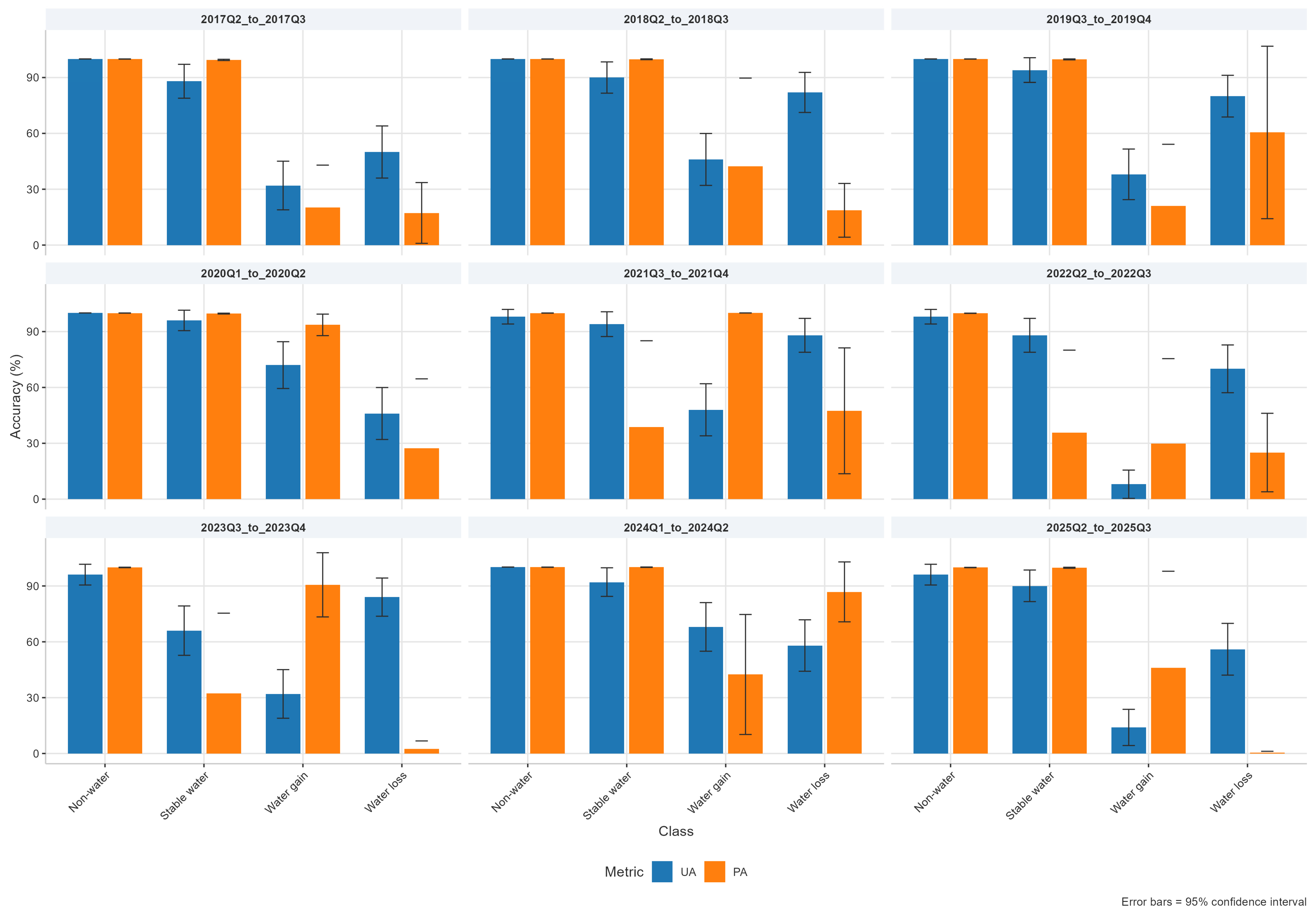
Figure A1. Class-wise User and Producer accuracy for each validated period.
Remotesensing 18 02075 g0a1
Figure A2. Confusion Matrix counts: 2017 Q2 to 2017 Q3.
Remotesensing 18 02075 g0a2
Figure A3. Confusion Matrix counts: 2018 Q2 to 2018 Q3.
Remotesensing 18 02075 g0a3
Figure A4. Confusion Matrix counts: 2019 Q3 to 2019 Q4.
Remotesensing 18 02075 g0a4
Figure A5. Confusion Matrix counts: 2020 Q1 to 2020 Q2.
Remotesensing 18 02075 g0a5
Figure A6. Confusion Matrix counts: 2021 Q3 to 2021 Q4.
Remotesensing 18 02075 g0a6
Figure A7. Confusion Matrix counts: 2022 Q2 to 2022 Q3.
Remotesensing 18 02075 g0a7
Figure A8. Confusion Matrix counts: 2023 Q3 to 2023 Q4.
Remotesensing 18 02075 g0a8
Figure A9. Confusion Matrix counts: 2024 Q1 to 2024 Q2.
Remotesensing 18 02075 g0a9
Figure A10. Confusion Matrix counts: 2025 Q2 to 2025 Q3.
Remotesensing 18 02075 g0a10

Appendix E

Mean River Metric Values

Table A4. Table showing all mean values of each planform river metric based on time series data.
Sub-BasinMean Channel
Width (m)
Mean Migration
Rate (m/q)
Mean
Sinuosity
Mean Stable
Water Area (m2)
Mean Water
Gain Area (m2)
Mean Water
Loss Area (m2)
Mean Stable
Water per km2
Mean Water
Gain per km2
Mean Water
Loss per km2
Abacaxis534.807.011.682,644,617,245.1049,277,911.1947,391,847.8820,714.42385.97371.20
Amazon floodplain2378.4767.021.5252,531,183,009.601,220,865,933.171,215,559,228.48132,599.613081.713068.32
Coastal basins north380.653.382.292,201,503,930.43154,905,244.80162,503,723.2519,644.831382.271450.08
Coastal basins south1022.8421.091.429,410,140,596.801,256,341,484.82944,051,271.5334,406.144593.543451.71
Japurá-Caquetá377.654.211.423,268,852,106.3054,416,256.9946,024,632.3312,869.44214.23181.19
Javari96.042.342.64546,134,404.639,008,187.359,065,386.525050.7183.3083.83
Juruá140.284.842.581,789,581,162.0438,387,211.9040,271,930.209440.02202.49212.43
Madeira513.3612.891.5216,427,359,946.61,858,527,174.531,700,875,690.1512,412.641404.311285.19
Manacupuru863.2535.481.58475,476,841.3012,832,512.8714,005,774.8241,866.331129.911233.22
Marañón252.758.661.802,991,967,363.0058,639,080.2849,690,246.858223.32161.16136.57
Napo301.2510.051.711,541,915,456.1217,243,661.3913,811,432.3015,217.87170.18136.31
Negro588.8070.661.6314,200,758,359.30515,755,105.96512,949,688.0519,734.95716.75712.85
Parana Madeirinha396.7026.162.01988,588,488.3519,741,153.7821,233,128.9726,552.71530.23570.30
Purus336.523.542.673,596,715,522.54122,990,701.19128,971,871.379727.65332.63348.81
Putumayo-Içá277.043.132.031,968,931,095.6116,192,326.3014,366,363.9416,584.04136.38121.01
Rio Araua1786.9724.932.191,422,015,442.0917,875,220.4719,179,761.9723,651.07297.30318.99
Rio Capim259.563.172.36650,107,245.08146,702,962.85108,959,647.078935.722016.431497.65
Rio Curuatingua336.826.171.50177,106,741.8340,802,299.6234,418,985.765749.631324.611117.38
Rio Jutai138.672.292.12754,795,317.7711,481,933.299,054,872.188433.71128.29101.17
Rio Nanay177.803.552.60102,197,680.031,673,470.531,414,736.926087.6199.6884.27
Rio Pacaja1343.922.101.551,072,074,342.5687,905,781.3764,307,399.2021,894.741795.281313.33
Rio Paru179.278.401.35587,702,215.4927,483,730.6626,195,278.654361.58203.96194.40
Rio Piorini1234.9129.841.57208,277,440.304,209,084.734,467,380.8324,752.01500.21530.91
Rio Uatuma762.049.501.903,691,449,219.6147,065,364.8038,664,171.7150,148.39639.38525.25
Tapajos1978.8411.701.587,427,889,003.40247,214,984.08190,728,963.9015,013.63499.68385.51
Tocantins802.995.591.3412,204,077,104.00885,474,873.17692,600,562.9015,845.231149.66899.24
Trombetas371.6010.131.501,592,253,890.0927,853,493.5225,361,964.1010,565.45184.82168.29
Ucayali281.45293.941.993,345,708,540.2179,845,473.1176,259,666.649433.55225.13215.02
Xingu1054.6496.811.486,262,088,105.67346,051,617.93276,130,666.6112,303.65679.92542.54

References

  1. Maciel, D.A.; Lousada, F.; Fassoni-Andrade, A.; Pacheco Quevedo, R.; Barbosa, C.C.F.; Paule-Bonnet, M.; Novo, E.M.L.d.M. Sentinel-1 Data Reveals Unprecedented Reduction of Open Water Extent Due to 2023–2024 Drought in the Central Amazon Basin. Environ. Res. Lett. 2024, 19, 124034. [Google Scholar] [CrossRef]
  2. Vital, H.; Stattegger, K.; Posewang, J.; Theilen, F. Lowermost Amazon River: Morphology and Shallow Seismic Characteristics. Mar. Geol. 1998, 152, 277–294. [Google Scholar] [CrossRef]
  3. Angulo, K.G.; Lee, K.T. Detecting the Planform Changes Due to the Seasonal Flow Fluctuation and 2012 Severe Flood in the Amazon River near Iquitos City, Peru Based on Remote Sensing Image Analysis. Water 2022, 14, 509. [Google Scholar] [CrossRef]
  4. Abad, J.D.; Garcia, A.P.; Marín-Díaz, J.; Escobar, C.; Ortals, C.; Chicchon, H. Morphodynamics of Anabranching Structures in the Peruvian Amazon River. Earth Surf. Process. Landf. 2024, 50, e6020. [Google Scholar] [CrossRef]
  5. Mendoza, A.; Abad, J.D.; Frias, C.E.; Ortals, C.; Paredes, J.; Montoro, H.; Vizcarra, J.; Simon, C.; Soto-Cortés, G. Planform Dynamics of the Iquitos Anabranching Structure in the Peruvian Upper Amazon River. Earth Surf. Process. Landf. 2016, 41, 961–970. [Google Scholar] [CrossRef]
  6. Nagel, G.W.; Darby, S.E.; Leyland, J. The Use of Satellite Remote Sensing for Exploring River Meander Migration. Earth-Sci. Rev. 2023, 247, 104607. [Google Scholar] [CrossRef]
  7. Venticinque, E.; Forsberg, B.; Barthem, R.; Petry, P.; Hess, L.; Mercado, A.; Cañas, C.; Montoya, M.; Durigan, C.; Goulding, M. An Explicit GIS-Based River Basin Framework for Aquatic Ecosystem Conservation in the Amazon. Earth Syst. Sci. Data 2016, 8, 651–661. [Google Scholar] [CrossRef]
  8. Palma-Silva, L.; Rivera-Rondón, C.A.; Henao, E.; Duque, S.R.; Piovano, E.; Figueira, R.C.L.; Ferreira, P.A.L.; Mejia-Rocha, M.; García-Rodríguez, F. The Influence of Amazon River Connectivity to Littoral Meanders on Long-Term Carbon Accumulation: A Case Study of Lake Yahuarcaca. Sci. Total Environ. 2023, 905, 167873. [Google Scholar] [CrossRef] [PubMed]
  9. Salerno, L.; Vezza, P.; Perona, P.; Camporeale, C. Eco-Morphodynamic Carbon Pumping by the Largest Rivers in the Neotropics. Sci. Rep. 2023, 13, 5591. [Google Scholar] [CrossRef] [PubMed]
  10. Li, J.; Donselaar, M.E.; Hosseini Aria, S.E.; Koenders, R.; Oyen, A.M. Landsat Imagery-Based Visualization of the Geomorphological Development at the Terminus of a Dryland River System. Quat. Int. 2014, 352, 100–110. [Google Scholar] [CrossRef]
  11. Caputo, M.V. Stratigraphy, Tectonics, Paleoclimatology and Paleogeography of Northern Basins of Brazil. Doctoral Dissertation, University of California, Berkeley, CA, USA, 1984. [Google Scholar]
  12. Schwenk, J.; Lanzoni, S.; Foufoula-Georgiou, E. The Life of a Meander Bend: Connecting Shape and Dynamics via Analysis of a Numerical Model. J. Geophys. Res. Earth Surf. 2015, 120, 690–710. [Google Scholar] [CrossRef]
  13. Arnez Ferrel, K.R.; Nelson, J.M.; Shimizu, Y.; Kyuka, T. Past, Present and Future of a Meandering River in the Bolivian Amazon Basin. Earth Surf. Process. Landf. 2020, 46, 715–727. [Google Scholar] [CrossRef]
  14. Jodhani, K.H.; Patel, D.; Madhavan, N.; Soni, U.; Patel, H.; Singh, S.K. Channel Planform Dynamics Using Earth Observations across Rel River, Western India: A Synergetic Approach. Spat. Inf. Res. 2024, 32, 497–510. [Google Scholar] [CrossRef]
  15. Junk, W.; Piedade, M.T.; Wittmann, F.; Schöngart, J.; Parolin, P. Amazonian Floodplain Forests: Ecophysiology, Biodiversity and Sustainable Management; Springer: Dordrecht, The Netherlands, 2011. [Google Scholar]
  16. Rozo, M.G.; Nogueira, A.C.R.; Truckenbrodt, W. The Anastomosing Pattern and the Extensively Distributed Scroll Bars in the Middle Amazon River. Earth Surf. Process. Landf. 2012, 37, 1471–1488. [Google Scholar] [CrossRef]
  17. Constantine, J.A.; Dunne, T.; Ahmed, J.; Legleiter, C.; Lazarus, E.D. Sediment Supply as a Driver of River Meandering and Floodplain Evolution in the Amazon Basin. Nat. Geosci. 2014, 7, 899–903. [Google Scholar] [CrossRef]
  18. Christopherson, R.W.; Birkeland, G.H. River Systems. In Geosystems, An Introduction to Physical Geography; Pearson Education Limited: Harlow, UK, 2015; Volume 9, pp. 448–481. [Google Scholar]
  19. Rowland, J.C.; Shelef, E.; Pope, P.A.; Muss, J.; Gangodagamage, C.; Brumby, S.P.; Wilson, C.J. A Morphology Independent Methodology for Quantifying Planview River Change and Characteristics from Remotely Sensed Imagery. Remote Sens. Environ. 2016, 184, 212–228. [Google Scholar] [CrossRef]
  20. Pappas, O.A.; Anantrasirichai, N.; Achim, A.M.; Adams, B.A. River Planform Extraction from High-Resolution SAR Images via Generalized Gamma Distribution Superpixel Classification. IEEE Trans. Geosci. Remote Sens. 2021, 59, 3942–3955. [Google Scholar] [CrossRef]
  21. Hamidi, E.; Peter, B.G.; Munoz, D.F.; Moftakhari, H.; Moradkhani, H. Fast Flood Extent Monitoring With SAR Change Detection Using Google Earth Engine. IEEE Trans. Geosci. Remote Sens. 2023, 61, 4201419. [Google Scholar] [CrossRef]
  22. Isikdogan, F.; Bovik, A.; Passalacqua, P. RivaMap: An Automated River Analysis and Mapping Engine. Remote Sens. Environ. 2017, 202, 88–97. [Google Scholar] [CrossRef]
  23. Tobón-Marín, A.; Cañón Barriga, J. Analysis of Changes in Rivers Planforms Using Google Earth Engine. Int. J. Remote Sens. 2020, 41, 8654–8681. [Google Scholar] [CrossRef]
  24. Uddin, M.M.; Bodruddoza Mia, M.; Gazi, M.Y.; Maksud Kamal, A.S.M. Quantification of Landuse Changes Driven by the Dynamics of the Jamuna River, a Giant Tropical River of Bangladesh. Egypt. J. Remote Sens. Space Sci. 2024, 27, 392–402. [Google Scholar] [CrossRef]
  25. Clement, M.A.; Kilsby, C.G.; Moore, P. Multi-Temporal Synthetic Aperture Radar Flood Mapping Using Change Detection. J. Flood Risk Manag. 2017, 11, 152–168. [Google Scholar] [CrossRef]
  26. Tran, K.H.; Menenti, M.; Jia, L. Surface Water Mapping and Flood Monitoring in the Mekong Delta Using Sentinel-1 SAR Time Series and Otsu Threshold. Remote Sens. 2022, 14, 5721. [Google Scholar] [CrossRef]
  27. Cerbelaud, A.; David, C.H.; Pavelsky, T.; Biancamaria, S.; Garambois, P.A.; Kittel, C.; Papa, F.; Bates, P.; Tourian, M.J.; Durand, M.; et al. Satellite Requirements to Capture Water Propagation in Earth’s Rivers. Rev. Geophys. 2025, 63, e2024RG000871. [Google Scholar] [CrossRef]
  28. Lang, F.; Zhu, Y.; Zhao, J.; Hu, X.; Shi, H.; Zheng, N.; Zha, J. Flood Mapping of Synthetic Aperture Radar (SAR) Imagery Based on Semi-Automatic Thresholding and Change Detection. Remote Sens. 2024, 16, 2763. [Google Scholar] [CrossRef]
  29. Marchetti, G.; Manconi, A.; Comiti, F. Limitations in the Use of Sentinel-1 Data for Morphological Change Detection in Rivers. Int. J. Remote Sens. 2023, 44, 6642–6669. [Google Scholar] [CrossRef]
  30. Khan, A.; Govil, H.; Khan, H.H.; Kumar Thakur, P.; Yunus, A.P.; Pani, P. Channel Responses to Flooding of Ganga River, Bihar India, 2019 Using SAR and Optical Remote Sensing. Adv. Space Res. 2022, 69, 1930–1947. [Google Scholar] [CrossRef]
  31. Rossi, D.; Zolezzi, G.; Bertoldi, W.; Vitti, A. Monitoring Braided River-Bed Dynamics at the Sub-Event Time Scale Using Time Series of Sentinel-1 SAR Imagery. Remote Sens. 2023, 15, 3622. [Google Scholar] [CrossRef]
  32. Melancon, A.M.; Andrew, M.L.; Griffin, R.E.; Mecikalski, J.R.; Schultz, L.A.; Bell, J.R. Random Forest Classification of Inundation Following Hurricane Florence (2018) via L-Band Synthetic Aperture Radar and Ancillary Datasets. Remote Sens. 2021, 13, 5098. [Google Scholar] [CrossRef]
  33. Gao, S.; Li, Z.; Chen, M.; Lin, P.; Hong, Z.; Allen, D.; Neeson, T.; Hong, Y. Spatiotemporal Variability of Global River Extent and the Natural Driving Factors Revealed by Decades of Landsat Observations, GRACE Gravimetry Observations, and Land Surface Model Simulations. Remote Sens. Environ. 2021, 267, 112725. [Google Scholar] [CrossRef]
  34. Ahmad, W.; Kim, D. Estimation of Flow in Various Sizes of Streams Using the Sentinel-1 Synthetic Aperture Radar (SAR) Data in Han River Basin, Korea. Int. J. Appl. Earth Obs. Geoinf. 2019, 83, 101930. [Google Scholar] [CrossRef]
  35. Tsyganskaya, V.; Martinis, S.; Marzahn, P. Flood Monitoring in Vegetated Areas Using Multitemporal Sentinel-1 Data: Impact of Time Series Features. Water 2019, 11, 1938. [Google Scholar] [CrossRef]
  36. Zhang, X.; Liu, L.; Wu, C.; Chen, X.; Gao, Y.; Xie, S.; Zhang, B. Development of a Global 30m Impervious Surface Map Using Multisource and Multitemporal Remote Sensing Datasets with the Google Earth Engine Platform. Earth Syst. Sci. Data 2020, 12, 1625–1648. [Google Scholar] [CrossRef]
  37. Rosenqvist, J.; Rosenqvist, A.; Jensen, K.; McDonald, K. Mapping of Maximum and Minimum Inundation Extents in the Amazon Basin 2014-2017 with ALOS-2 PALSAR-2 Scan SAR Time-Series Data. Remote Sens. 2020, 12, 1326. [Google Scholar] [CrossRef]
  38. Aires, F.; Papa, F.; Prigent, C. A Long-Term, High-Resolution Wetland Dataset over the Amazon Basin, Downscaled from a Multiwavelength Retrieval Using SAR Data. J. Hydrometeorol. 2013, 14, 594–607. [Google Scholar] [CrossRef]
  39. Birkett, C.M.; Mertes, L.A.K.; Dunne, T.; Costa, M.H.; Jasinski, M.J. Surface Water Dynamics in the Amazon Basin: Application of Satellite Radar Altimetry. J. Geophys. Res. Atmos. 2002, 107, LBA 26-1–LBA 26-21. [Google Scholar] [CrossRef]
  40. Mitidieri, F.; Papa, M.N.; Amitrano, D.; Ruello, G. River Morphology Monitoring Using Multitemporal Sar Data: Preliminary Results. Eur. J. Remote Sens. 2016, 49, 889–898. [Google Scholar] [CrossRef]
  41. Arnesen, A.S.; Silva, T.S.F.; Hess, L.L.; Novo, E.M.L.M.; Rudorff, C.M.; Chapman, B.D.; McDonald, K.C. Monitoring Flood Extent in the Lower Amazon River Floodplain Using ALOS/PALSAR ScanSAR Images. Remote Sens. Environ. 2013, 130, 51–61. [Google Scholar] [CrossRef]
  42. Basnayaka, V.; Samarasinghe, J.T.; Gunathilake, M.B.; Muttil, N.; Rathnayake, U. Planform Changes in the Lower Mahaweli River, Sri Lanka Using Landsat Satellite Data. Land 2022, 11, 1716. [Google Scholar] [CrossRef]
  43. Vanderhoof, M.K.; Alexander, L.; Christensen, J.; Solvik, K.; Nieuwlandt, P.; Sagehorn, M. High-Frequency Time Series Comparison of Sentinel-1 and Sentinel-2 Satellites for Mapping Open and Vegetated Water across the United States (2017–2021). Remote Sens. Environ. 2023, 288, 113498. [Google Scholar] [CrossRef] [PubMed]
  44. Hou, J.; Van Dijk, A.I.J.M.; Renzullo, L.J.; Vertessy, R.A.R. Using Modelled Discharge to Develop Satellite-Based River Gauging: A Case Study for the Amazon Basin. Hydrol. Earth Syst. Sci. 2018, 22, 6435–6448. [Google Scholar] [CrossRef]
  45. Boothroyd, R.J.; Williams, R.D.; Barrett, B.; Hoey, T.B.; Tolentino, P.L.M.; Perez, J.E.; Guardian, E.; David, C.P.; Yang, X. Detecting and Quantifying Morphological Change in Tropical Rivers Using Google Earth Engine and Image Analysis Techniques; CRC Press: Boca Raton, FL, USA; Balkema: Rotterdam, The Netherland, 2020. [Google Scholar]
  46. Cerbelaud, A.; David, C.H.; Biancamaria, S.; Wade, J.; Tom, M.; Prata de Moraes Frasson, R.; Allen, G.H.; Thurman, H.; Blumstein, D. Spatial Hydrographs of River Flow and Their Analysis for Peak Event Detection in the Context of Satellite Sampling. Water Resour. Res. 2025, 61, e2024WR038444. [Google Scholar] [CrossRef]
  47. Latrubesse, E.M. Patterns of Anabranching Channels: The Ultimate End-Member Adjustment of Mega Rivers. Geomorphology 2008, 101, 130–145. [Google Scholar] [CrossRef]
  48. ESA Sentinel-1. Available online: https://documentation.dataspace.copernicus.eu/Data/SentinelMissions/Sentinel1.html (accessed on 31 March 2026).
  49. Google Developers Sentinel-1 Algorithms. Available online: https://developers.google.com/earth-engine/guides/sentinel1 (accessed on 31 March 2026).
  50. Mullissa, A.; Vollrath, A.; Odongo-Braun, C.; Slagter, B.; Balling, J.; Gou, Y.; Gorelick, N.; Reiche, J. Sentinel-1 Sar Backscatter Analysis Ready Data Preparation in Google Earth Engine. Remote Sens. 2021, 13, 1954. [Google Scholar] [CrossRef]
  51. Zanaga, D.; Van De Kerchove, R.; Daems, D.; De Keersmaecker, W.; Brockmann, C.; Kirches, G.; Wevers, J.; Cartus, O.; Santoro, M.; Fritz, S.; et al. ESA WorldCover 10 m 2021 V200. Available online: https://zenodo.org/records/7254221 (accessed on 31 March 2026).
  52. Van De Kerchove, R.; Zanaga, D.; Xu, P.; Tsendbazar, N.-E.; Lesiv, M. Product User Manual Document Ref: WorldCover_PUM_v2.0. 2022. Available online: https://pure.iiasa.ac.at/id/eprint/18983/ (accessed on 30 April 2026).
  53. Farr, T.G.; Rosen, P.A.; Caro, E.; Crippen, R.; Duren, R.; Hensley, S.; Kobrick, M.; Paller, M.; Rodriguez, E.; Roth, L.; et al. The Shuttle Radar Topography Mission. Rev. Geophys. 2007, 45, RG2004. [Google Scholar] [CrossRef]
  54. NASA. The Shuttle Radar Topography Mission (SRTM) Collection User Guide. Available online: https://lpdaac.usgs.gov/documents/179/SRTM_User_Guide_V3.pdf (accessed on 31 March 2026).
  55. Planet Labs PBC Planet Application Program Interface: In Space for Life on Earth. Available online: https://api.planet.com (accessed on 17 February 2026).
  56. Planet Labs PBC Mosaics. Available online: https://docs.planet.com/data/imagery/mosaics/ (accessed on 31 March 2026).
  57. Otsu, N. A Threshold Selection Method from Gray-Level Histograms. IEEE Trans. Syst. Man Cybern. 1979, 9, 62–66. [Google Scholar] [CrossRef]
  58. Olofsson, P.; Foody, G.M.; Herold, M.; Stehman, S.V.; Woodcock, C.E.; Wulder, M.A. Good Practices for Estimating Area and Assessing Accuracy of Land Change; Elsevier Inc.: San Diego, CA, USA, 2014; Volume 148. [Google Scholar]
  59. Tyukavina, A.; Stehman, S.V.; Pickens, A.H.; Potapov, P.; Hansen, M.C. Practical Global Sampling Methods for Estimating Area and Map Accuracy of Land Cover and Change. Remote Sens. Environ. 2025, 324, 114714. [Google Scholar] [CrossRef]
  60. Pickens, A.H.; Hansen, M.C.; Hancher, M.; Stehman, S.V.; Tyukavina, A.; Potapov, P.; Marroquin, B.; Sherani, Z. Mapping and Sampling to Characterize Global Inland Water Dynamics from 1999 to 2018 with Full Landsat Time-Series. Remote Sens. Environ. 2020, 243, 111792. [Google Scholar] [CrossRef]
  61. Schwenk, J.; Khandelwal, A.; Fratkin, M.; Kumar, V.; Foufoula-Georgiou, E. High Spatiotemporal Resolution of River Planform Dynamics from Landsat: The RivMAP Toolbox and Results from the Ucayali River. Earth Space Sci. 2017, 4, 46–75. [Google Scholar] [CrossRef]
  62. Pavelsky, T.M.; Smith, L.C. RivWidth: A Software Tool for the Calculation of River Widths from Remotely Sensed Imagery. IEEE Geosci. Remote Sens. Lett. 2008, 5, 70–73. [Google Scholar] [CrossRef]
  63. Zhang, F.; Sun, Q.; Wen, B.; Ma, J.; Lv, Z. Skeleton Line Extraction for Areal Hydrographic Elements Considering Spatial and Hierarchical Relationships. Geocarto Int. 2022, 37, 16398–16417. [Google Scholar] [CrossRef]
  64. Wei, Y.; Zhang, K.; Ji, S. Simultaneous Road Surface and Centerline Extraction from Large-Scale Remote Sensing Images Using CNN-Based Segmentation and Tracing. IEEE Trans. Geosci. Remote Sens. 2020, 58, 8919–8931. [Google Scholar] [CrossRef]
  65. Xue, Y.; Qin, C.; Wu, B.; Li, D.; Fu, X. Automatic Extraction of Mountain River Surface and Width Based on Multisource High-Resolution Satellite Images. Remote Sens. 2022, 14, 2370. [Google Scholar] [CrossRef]
  66. Li, Q.; Lan, H.; Zhao, X.; Wu, Y. River Centerline Extraction Using the Multiple Direction Integration Algorithm for Mixed and Pure Water Pixels. GIsci. Remote Sens. 2019, 56, 256–281. [Google Scholar] [CrossRef]
  67. Dijkstra, E.W. A Note on Two Problems in Connexion with Graphs. Numer. Math. 1959, 1, 269–271. [Google Scholar] [CrossRef]
  68. Wang, S.X. The Improved Dijkstra’s Shortest Path Algorithm and Its Application. In Proceedings of the Procedia Engineering; Elsevier Ltd.: Amsterdam, The Netherlands, 2012; Volume 29, pp. 1186–1190. [Google Scholar]
  69. Savitzky, A.; Golay, M.J.E. Smoothing and Differentiation of Data by Simplified Least Squares Procedures; American Chemical Society: Washington, DC, USA, 1964; Volume 40. [Google Scholar]
  70. Felzenszwalb, P.F.; Huttenlocher, D.P. Distance Transforms of Sampled Functions. Theory Comput. 2012, 8, 415–428. [Google Scholar] [CrossRef]
  71. Coe, M.T.; Costa, M.H.; Howard, E.A. Simulating the Surface Waters of the Amazon River Basin: Impacts of New River Geomorphic and Flow Parameterizations. Hydrol. Process. 2008, 22, 2542–2553. [Google Scholar] [CrossRef]
  72. Leopold, L.; Wolman, G.; Udall, S.L.; Nolan, T.B. River Channel Patterns: Braided, Meandering and Straight; U.S. Governmental Print Office: Washington, DC, USA, 1957.
  73. Hooke, J.M. River Meandering. In Treatise on Geomorphology: Volume 1–14; Elsevier: Amsterdam, The Netherlands, 2013; Volume 1–14, pp. 260–288. [Google Scholar]
  74. Schwenk, J.; Foufoula-Georgiou, E. Meander Cutoffs Nonlocally Accelerate Upstream and Downstream Migration and Channel Widening. Geophys. Res. Lett. 2016, 43, 12,437–12,445. [Google Scholar] [CrossRef]
  75. Bentley, J.L. Multidimensional Binary Search Trees Used for Associative Searching. Commun. ACM 1975, 18, 509–517. [Google Scholar] [CrossRef]
  76. Legleiter, C.J. A Geostatistical Framework for Quantifying the Reach-Scale Spatial Structure of River Morphology: 1. Variogram Models, Related Metrics, and Relation to Channel Form. Geomorphology 2014, 205, 65–84. [Google Scholar] [CrossRef]
  77. Vercruysse, K.; Grabowski, R.C. Human Impact on River Planform within the Context of Multi-Timescale River Channel Dynamics in a Himalayan River System. Geomorphology 2021, 381, 107659. [Google Scholar] [CrossRef]
  78. Kuo, C.W.; Chen, C.F.; Chen, S.C.; Yang, T.C.; Chen, C.W. Channel Planform Dynamics Monitoring and Channel Stability Assessment in Two Sediment-Rich Rivers in Taiwan. Water 2017, 9, 84. [Google Scholar] [CrossRef]
  79. Rozo, M.G.; Nogueira, A.C.R.; Castro, C.S. Remote Sensing-Based Analysis of the Planform Changes in the Upper Amazon River over the Period 1986–2006. J. S. Am. Earth Sci. 2014, 51, 28–44. [Google Scholar] [CrossRef]
  80. Gutierrez, R.R.; Abad, J.D.; Choi, M.; Montoro, H. Characterization of Confluences in Free Meandering Rivers of the Amazon Basin. Geomorphology 2014, 220, 1–14. [Google Scholar] [CrossRef]
  81. Snyder, H. Literature Review as a Research Methodology: An Overview and Guidelines. J. Bus. Res. 2019, 104, 333–339. [Google Scholar] [CrossRef]
  82. Shrestha, P.; Tamrakar, N.K. Morphology and Classification of the Main Stem Bagmati River, Central Nepal. Bull. Dep. Geol. Tribhuvan Univ. Kathmandu Nepal 2013, 15, 23–24. [Google Scholar] [CrossRef]
  83. Greenberg, E.; Chadwick, A.J.; Li, G.K.; Ganti, V. Quantifying Channel Mobility and Floodplain Reworking Timescales Across River Planform Morphologies. Geophys. Res. Lett. 2024, 51, e2024GL108537. [Google Scholar] [CrossRef]
  84. Li, Y.; Zhang, Y.; Zheng, N.; Li, L.; Ji, H.; Bao, Z.; Feng, Z. Global Classification of River Morphology Based on Inland Water Dynamics Characterization and Digital Elevation Data. Sci. Rep. 2025, 15, 14258. [Google Scholar] [CrossRef] [PubMed]
  85. Connor-Streich, G.; Henshaw, A.J.; Brasington, J.; Bertoldi, W.; Harvey, G.L. Let’s Get Connected: A New Graph Theory-Based Approach and Toolbox for Understanding Braided River Morphodynamics. Wiley Interdiscip. Rev. Water 2018, 5, e1296. [Google Scholar] [CrossRef]
  86. Schwanghart, W.; Molkenthin, C.; Scherler, D. A Systematic Approach and Software for the Analysis of Point Patterns on River Networks. Earth Surf. Process. Landf. 2021, 46, 1847–1862. [Google Scholar] [CrossRef]
  87. Lane, S.N.; Richards, K.S.; Chandler, J.H. Developments in Monitoring and Modelling Small-scale River Bed Topography. Earth Surf. Process. Landf. 1994, 19, 349–368. [Google Scholar] [CrossRef]
  88. Nogueira, X.R.; Pasternack, G.B.; Lane, B.A.; Sandoval-Solis, S. Width Undulation Drives Flow Convergence Routing in Five Flashy Ephemeral River Types across a Dry Summer Subtropical Region. Earth Surf. Process. Landf. 2024, 49, 1890–1913. [Google Scholar] [CrossRef]
  89. Corenblit, D.; Steiger, J. Fluvial Biogeomorphological Feedbacks from Plant Traits to the Landscape: Lessons from Selected French Rivers in Line with A.M. Gurnell’s Influential Contribution. In Proceedings of the River Research and Applications; John Wiley and Sons Ltd.: Hoboken, NJ, USA, 2024; Volume 40, pp. 1012–1030. [Google Scholar]
  90. White, J.S.; Bartelt, K.; Overstreet, B.T.; Kelley, J.R. High Resolution Mapping of Submerged Sediment Size and Suitable Salmon Spawning Habitat Using Topo-Bathymetric Lidar in the Santiam River Basin, Oregon. Water Resour. Res. 2025, 61, e2024WR039219. [Google Scholar] [CrossRef]
  91. Ashmore, P.; Peirce, S.; Leduc, P. Expanding the “Active Layer”: Discussion of Church and Haschenburger (2017) What Is the “Active Layer”? Water Resources Research 53, 5–10. Doi:10.1002/2016WR019675. Water Resour. Res. 2018, 54, 1425–1427. [Google Scholar] [CrossRef]
  92. Thoms, M.; Scown, M.; Flotemersch, J. Characterization of River Networks: A GIS Approach and Its Applications. J. Am. Water Resour. Assoc. 2018, 54, 899–913. [Google Scholar] [CrossRef] [PubMed]
  93. Arnaud-Fassetta, G.; Melun, G.; Passy, P.; Brousse, G.; Theureaux, O. How to Quantify the Dynamics of Single (Straight or Sinuous) and Multiple (Anabranching) Channels from Imagery for River Restoration. Appl. Sci. 2021, 11, 8075. [Google Scholar] [CrossRef]
  94. Wohl, E.; Brierley, G.; Cadol, D.; Coulthard, T.J.; Covino, T.; Fryirs, K.A.; Grant, G.; Hilton, R.G.; Lane, S.N.; Magilligan, F.J.; et al. Connectivity as an Emergent Property of Geomorphic Systems. Earth Surf. Process. Landf. 2019, 44, 4–26. [Google Scholar] [CrossRef]
  95. Nones, M.; Archetti, R.; Guerrero, M. Time-Lapse Photography of the Edge-of-Water Line Displacements of a Sandbar as a Proxy of Riverine Morphodynamics. Water 2018, 10, 617. [Google Scholar] [CrossRef]
  96. von Suchodoletz, H.; Pohle, M.; Khosravichenar, A.; Ulrich, M.; Hein, M.; Tinapp, C.; Schultz, J.; Ballasus, H.; Veit, U.; Ettel, P.; et al. The Fluvial Architecture of Buried Floodplain Sediments of the Weiße Elster River (Germany) Revealed by a Novel Method Combination of Drill Cores with Two-Dimensional and Spatially Resolved Geophysical Measurements. Earth Surf. Process. Landf. 2022, 47, 955–976. [Google Scholar] [CrossRef]
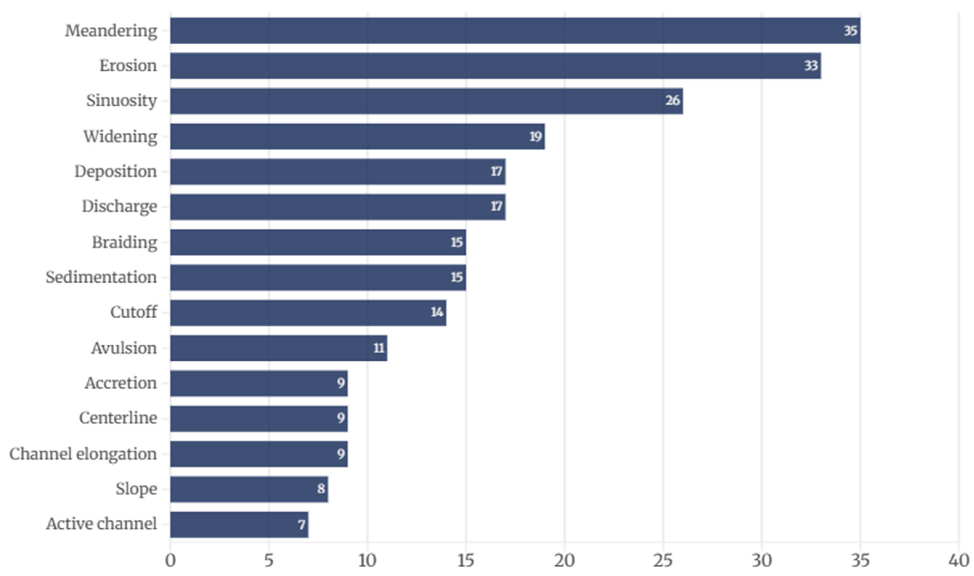
Figure 1. Top 15 most used planform river dynamics sorted by count based on the author’s semi-systematic literature review of 60 peer-reviewed sources.
Remotesensing 18 02075 g001
Figure 2. Percentage of most used remote sensing and other sensors in literature based on 60 reviewed sources. Spectral is the most used remote sensing sensor with 66.7%. The “other sensors” category consists of non-remote sensing methods such as tacheometry, photography, water level gauging, sonar, kinematic DGPS and hydrometers.
Remotesensing 18 02075 g002
Figure 3. (A) Study area reference within the continent of South America. (B) Twenty nine BL2 hydrological Amazonian sub-basins, based on Venticinque et al. [7]. (C) Geotectonic units of the Amazon Basin: Acre, Solimões, Amazonas and Marajó basins, modified from Rozo et al. [16].
Remotesensing 18 02075 g003
Figure 4. Areas with missing SAR data marked in red, due to Sentinel-1B failure from 2022 Q1 to 2024 Q4. (i) shows northern data-gap removing parts of the Japurá—Caquetá and Negro sub-basins; (ii) shows southern data-gap removing parts of the Madeira sub-basin.
Remotesensing 18 02075 g004
Figure 5. Flowchart of the methodology, including data input, pre-processing in GEE, water classification in GEE, post-processing in Python (v3.13) and validation in QGIS (v3.40.12) and R (v4.4.2), for a larger version of this figure see Supplement S1.
Remotesensing 18 02075 g005
Figure 6. Graph showing the distribution of VH backscatter values (in dB) and the fixed histogram threshold (green) and Otsu threshold (red).
Remotesensing 18 02075 g006
Figure 7. (A1) PlanetScope satellite imagery of a turbulent water surface and (B1) of an anastomosing river pattern. (A2,B2) Water classification using the fixed histogram threshold and (A3,B3) water classification using Otsu. (A2,B2) More gaps and inconsistencies in water classification than (A3,B3).
Remotesensing 18 02075 g007
Figure 8. (A) ESA WorldCover 10 m v200 dataset. (B) Water classification using the Otsu threshold without implementing a landcover filter, where all blue areas are water and white areas are non-water. (C) Water classification using the Otsu threshold with the landcover-based filter.
Remotesensing 18 02075 g008
Figure 9. (A) PlanetScope satellite imagery of a section of the Rio Branco in Boa Vista where a bridge and a patch of bare soil are visible. (B) Raw water mask as exported from GEE. (C) Water mask after applying the majority filter. (D) Water mask after applying the gap-filling filter.
Remotesensing 18 02075 g009
Figure 10. Flowchart showing planform river metric extraction steps, such as preparation, centerline extraction and metric calculation, for a larger version of this figure see Supplement S2.
Remotesensing 18 02075 g010
Figure 11. Boxplots showing all water-change classes and their respective User and Producer accuracies across all periods (nine per class).
Remotesensing 18 02075 g011
Figure 12. All generated centerlines of each Amazon tributary mainstem of 2019 Q2 and their respective basins.
Remotesensing 18 02075 g012
Figure 13. (A) Example of the Marañón (upstream) river and its centerlines, with (ai) spectral reference at 20,017—Q1 and (bi) at 2025—Q4. (B) Example of the Xingu (downstream) river and its centerlines, with (aii) spectral reference at 20,017—Q1 and (bii) at 2025—Q4. (C) Example of the Juruá (middle) river and its centerlines, with (aiii) spectral reference at 20,017—Q1 and (biii) at 2025—Q4. For each example, PlanetScope imagery is provided from the beginning and the end of the monitoring period.
Remotesensing 18 02075 g013
Figure 14. Mean of the six river metrics for each Amazon sub-basin: (A) Mean channel width. (B) Mean migration rate. (C) Mean sinuosity. (D) Mean stable water area. (E) Mean water gain area. (F) Mean water loss area.
Remotesensing 18 02075 g014
Disclaimer/Publisher’s Note: The statements, opinions and data contained in all publications are solely those of the individual author(s) and contributor(s) and not of MDPI and/or the editor(s). MDPI and/or the editor(s) disclaim responsibility for any injury to people or property resulting from any ideas, methods, instructions or products referred to in the content.