CSD-Net: Content–Style Decoupling with Exploratory MLLM-Guided Refinement for Robust Change Detection

Highlights

What are the main findings?

• CSD-Net introduces a style-aware content–style decoupling mechanism with pseudo-change tokens to reduce seasonal, illumination, and atmospheric pseudo-changes in remote sensing change detection.
• Across four benchmark datasets, CSD-Net (Base) achieves a strong accuracy–efficiency trade-off, while the optional MLLM+SAM refinement further improves uncertain hard cases in offline scenarios.

What are the implications of the main findings?

• The proposed framework provides an efficient and robust base detector suitable for large-scale bi-temporal remote sensing change detection with radiometric and environmental variations.
• The coarse-to-fine refinement strategy shows that foundation models can be used as optional semantic refiners for quality-critical applications without replacing the lightweight base detector.

Abstract

Remote sensing change detection (RSCD) aims to produce pixel-accurate change maps from bi-temporal images yet is fundamentally challenged by radiometric pseudo-changes (season, illumination, and atmosphere) that cause structure–environment entanglement in deep features. We propose CSD-Net, a framework centered on content–style decoupling (CSD): a physics-inspired feature decomposition mechanism that encourages separation between intrinsic geometric content and extrinsic environmental style. In the CSD module, learnable pseudo-change tokens estimate a spatially invariant global style proxy through cross-attention and broadcast, and subtraction performs feature-level radiometric-bias compensation, yielding pseudo-change-robust content features for change prediction. CSD-Net (Base) alone achieves state-of-the-art performance across four benchmarks (LEVIR-CD, LEVIR-CD+, CDD, and WHU) with favorable accuracy–efficiency trade-off (14.49M parameters and 15.26G FLOPs). We further explore an optional extension, CSD-Net⁺, that employs an MLLM (Qwen2.5-3B, LoRA-tuned) as a semantic refiner and SAM for instance mask refinement, coupled with uncertainty-aware three-way softmax fusion. This exploratory Stage 2 brings modest but consistent IoU improvements of 0.45–2.20% at the cost of significant computational overhead and is designed for offline, quality-critical scenarios. We provide a comprehensive account of both the effectiveness and the limitations of the proposed approach, including the marginal benefit–cost ratio of foundation model integration.

1. Introduction

Remote sensing change detection (RSCD) aims to infer semantic change (what humans care about) from radiometric change (what sensors measure) across time. This mismatch makes RSCD intrinsically ill-posed: similar radiometric differences may correspond to no semantic change (e.g., season/illumination), while subtle semantic changes may induce weak radiometric signals. Consequently, many detectors break down because they implicitly rely on a flawed premise—feature distance ≈ semantic change—without explicitly modeling radiometric bias and intrinsic/extrinsic factors.

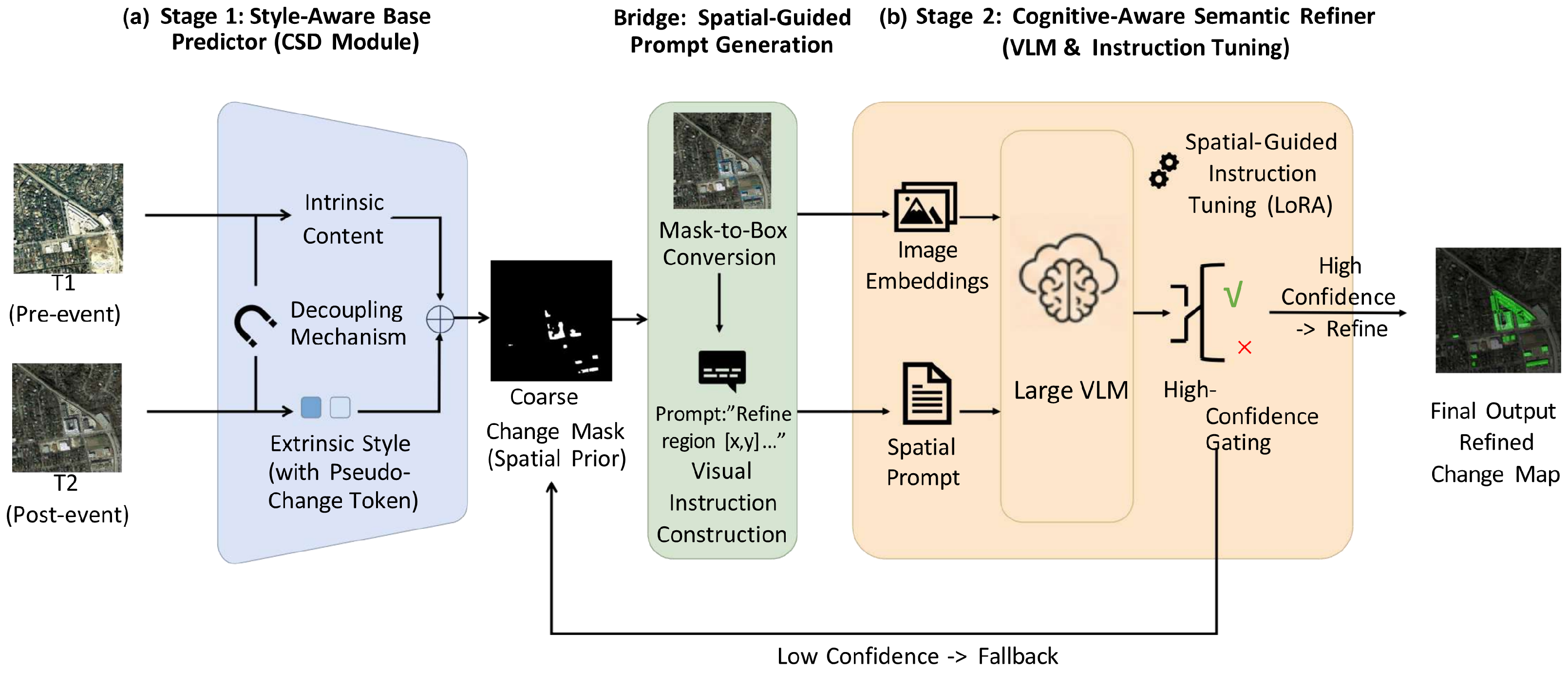
The above conflict manifests as two coupled scientific challenges. First, standard pixel-level matching is vulnerable to global radiometric bias (phenology, illumination, and atmosphere), leading to structure–environment entanglement and pseudo-change false alarms. Second, even when radiometric bias is controlled, purely visual features are sometimes insufficient for semantically ambiguous regions (e.g., barren land vs. construction site), where resolving “change” requires world knowledge and cognitive reasoning beyond appearance. This motivates a principled coarse-to-fine solution: encourage a physics-inspired intrinsic/extrinsic feature decomposition for robust localization, and invoke an MLLM as a semantic refiner only on hard, uncertain regions. An overview is provided in Figure 1.

In the past decade, deep learning has revolutionized RSCD, establishing Convolutional Neural Networks (CNNs) as the dominant paradigm. Pioneering works such as FC-Siam-Di [1] and UNet++ [2] introduced Siamese architectures to extract multi-scale features for pixel-wise comparison. To further enhance feature discriminability, attention mechanisms were incorporated. For instance, DASNet [3] and STANet [4] utilized spatial-temporal attention to model contextual relationships, significantly improving performance. However, CNNs inherently struggle with modeling long-range dependencies due to their limited receptive fields. To address this, the community has recently shifted towards transformer-based architectures. Methods like BIT [5], ChangeFormer [5], and SwinSUNet [6] leverage self-attention mechanisms to capture global context, achieving new state-of-the-art (SOTA) results.

Despite these advancements, most existing CNN and transformer-based methods (which we refer to as specialized “small models”) operate on a fundamental assumption: that feature distance directly correlates with semantic change. In reality, “content” (the semantic object, e.g., a building) and “style” (the environmental appearance, e.g., color, lighting) are often entangled in the feature space. Without an explicit mechanism to reduce this entanglement, models are prone to generating false alarms in regions with strong style shifts (e.g., vegetation turning yellow in winter) while missing subtle semantic changes. This limitation highlights the need for a mechanism that encourages separation between intrinsic content and extrinsic style.

Parallel to the development of specialized RSCD models, the computer vision community has witnessed a paradigm shift driven by Vision–Language Models (VLMs) and Large Multimodal Models (LMMs). Models like CLIP [7] have demonstrated exceptional zero-shot generalization and semantic reasoning capabilities by aligning visual features with rich textual semantics. In the remote sensing domain, recent works have attempted to leverage these foundation models. For example, ChangeCLIP [8] attempts to transfer the capabilities of CLIP to change detection by aligning visual features with text prompts. However, directly applying general-purpose VLMs to RSCD faces a critical “granularity gap”: VLMs excel at image-level or object-level semantic reasoning (answering “what” has changed) but often lack the pixel-level spatial precision required for dense change maps (answering exactly “where” the boundary lies). Furthermore, fine-tuning large models on limited remote sensing data often leads to catastrophic forgetting or suboptimal localization, making them less effective than specialized small models in pixel-wise metrics.

Encouragingly, powerful remote sensing foundation models have started to emerge. Vision backbones pretrained with masked image modeling, such as RingMo [9], substantially strengthen feature representation and transferability. Meanwhile, remote sensing MLLMs (e.g., GeoChat [10] and SkySense [11]) demonstrate impressive open-vocabulary understanding and instruction-following ability. However, directly adopting these general-purpose models for RSCD remains non-trivial: many are text-centric or focus on single-image understanding (e.g., RSGPT [12]), and even grounding-enabled models typically output box-level localization (e.g., GeoChat [10]), which falls short of the strict pixel-wise boundary accuracy required for mapping-grade change maps. To bridge this gap, we propose a data transformation + instruction tuning strategy: we convert RSCD supervision into refinement-style multimodal instructions and perform supervised LoRA-based adaptation of the MLLM. This allows CSD-Net to inherit the reasoning capability of large models while explicitly aligning them with the dense prediction requirement of RSCD.

To bridge the gap between specific pixel-level precision and generalized semantic reasoning, we argue that a robust RSCD system can benefit from a coarse-to-fine synergy: a specialized small model localizes potential changes from dense visual features, and an optional large-model refiner classifies difficult proposals with semantic context.

In this paper, we propose CSD-Net, a unified framework that integrates content–style decoupling with spatially guided visual instruction tuning for robust change detection. Our approach addresses the aforementioned challenges in two progressive stages:

First, recognizing that pseudo-changes are the primary bottleneck for pixel-level accuracy, we constructed a lightweight yet powerful base predictor: the content–style decoupling module. Unlike previous methods that treat features as a whole, we introduce learnable “pseudo-change tokens” to model extrinsic style variations as a compact global proxy. In particular, we constrain the style map to be spatially invariant via global pooling and broadcast so that the subtraction operation acts as feature-level compensation for dominant global radiometric/style shifts. By encouraging the network to separate intrinsic content from extrinsic style in a dual-decoder structure, CSD-Net establishes a strong baseline that suppresses many false alarms caused by environmental factors.

Second, to address the semantic ambiguity in hard cases (e.g., distinguishing construction sites from barren land), we incorporate an MLLM as a semantic refiner, specifically a Qwen2.5-3B multimodal model initialized from Rex-Omni weights [13], coupled with SAM [14] for pixel-accurate mask refinement. Instead of using the MLLM as a simple feature extractor, we propose a spatially guided visual instruction tuning strategy. We transform uncertain regions from the base model into coarse proposal boxes. These boxes serve as “visual instructions,” guiding the MLLM to generate refined box coordinates and predict change or no-change with confidence scores. The refined positive boxes are then converted by SAM into pixel-accurate instance masks with sharp boundaries. Crucially, we designed a three-way uncertainty-aware softmax fusion mechanism that integrates the base prior, SAM-refined positive evidence (for false negative recovery), and refined negative evidence (for false positive suppression), with weights dynamically controlled by pixel-wise entropy. This ensures that Stage 2 corrections are selectively applied in uncertain regions while preserving the base model’s precision in confident areas.

The main contributions of this article are summarized as follows:

• We propose CSD-Net, a novel coarse-to-fine framework that synergizes the spatial precision of specialized small models with the semantic reasoning of MLLMs and the boundary accuracy of SAM [14] through a three-way uncertainty-aware softmax fusion mechanism.
• We introduce a content–style decoupling mechanism for the base predictor, employing learnable pseudo-change tokens to encourage separation between global style factors (e.g., seasonal tone and illumination) and semantic content, achieving strong performance competitive with or surpassing previous methods.
• We designed a spatially guided visual instruction tuning strategy with SAM-based instance mask refinement. The base model generates coarse proposal boxes from uncertain regions; a semantic refiner (Rex-Omni-R) outputs refined box coordinates and predicts change/no-change with confidence; SAM then converts positively refined boxes into pixel-accurate instance masks with sharp boundaries. A novel three-way softmax fusion integrates positive evidence ${\mathbf{M}}_{+}$ (SAM-refined masks), negative evidence ${\mathbf{M}}_{-}$ (refined no-change regions), and the base prior ${\mathbf{P}}_{\mathrm{base}}$, enabling simultaneous false negative recovery and false positive suppression.
• Extensive experiments on four benchmarks (LEVIR-CD [4], LEVIR-CD+, CDD [15], and WHU [16]) demonstrate that CSD-Net (Base) already achieves state-of-the-art accuracy–efficiency trade-off among pure-vision detectors. The exploratory MLLM+SAM extension provides additional but modest gains (0.45–2.20% IoU) at higher computational cost and is positioned as an optional offline refinement module for quality-critical scenarios.

To place our contributions in context, we review related work along two complementary directions: (i) specialized RSCD “small models” that pursue pixel-level precision but remain sensitive to radiometric bias and structure–environment entanglement and (ii) VLM/MLLM-based perception models that provide cognitive reasoning yet lack dense pixel-level granularity. This perspective clarifies the motivation of combining style-aware feature decomposition with spatially guided semantic refinement in CSD-Net.

2. Related Work

2.1. Remote Sensing Change Detection

From the viewpoint of the radiometric–semantic mismatch, most RSCD studies can be seen as progressively improving pixel-wise matching under increasingly complex imaging conditions. Traditional remote sensing image change detection (RSICD) relied heavily on handcrafted spectral difference analysis, such as Change Vector Analysis (CVA) and post-classification comparison [17], which, however, struggled with noise sensitivity and high-resolution data complexity. The paradigm shift to deep learning established Siamese Convolutional Neural Networks (CNNs) as the standard, where methods like FC-Siam-Di [1] and CDNet [18] utilized shared encoders for discriminative feature extraction. To overcome the limitation of local receptive fields in CNNs, subsequent works incorporated attention mechanisms and multi-scale aggregation strategies. For instance, STANet [4] captured spatial-temporal dependencies, while DMATNet [19] and ICIF-Net [20] refined boundaries through feature interaction. Recently, transformer-based architectures [5,6,21] and State Space Models (SSMs) like RS-Mamba [22] and CDMamba [23] have further pushed the performance envelope by modeling global context.

Nevertheless, these feature-distance-based methods often operate on the assumption that feature disparity equals semantic change, leaving them vulnerable to pseudo-changes caused by seasonal or atmospheric variations. Recognizing this entanglement between semantic content and environmental style, recent studies have pivoted towards feature decoupling and consistency modeling. Approaches such as LGPNet [24], RCCD [25], and APD [26] explicitly suppress time-specific noise or separate content-agnostic features, suggesting that style-aware feature separation is useful for robustness. Concurrently, vision–language pre-training has inspired methods like ChangeCLIP [8] to leverage multimodal semantic alignment. However, general VLMs [27,28] often suffer from a “granularity gap” in dense pixel-wise prediction, motivating our coarse-to-fine strategy that combines style-aware base prediction with spatially guided semantic refinement.

2.2. Generative Detection in Multimodal LLMs

Complementary to small-model advances, MLLMs offer a different axis of progress: they inject world knowledge and cognitive reasoning into visual understanding, which is crucial for resolving semantically ambiguous regions beyond appearance cues. The rapid evolution of Multimodal Large Language Models (MLLMs) has extended their capabilities from general image understanding to fine-grained perception tasks, including object detection and grounding [29]. Diverging from traditional closed-set detectors, MLLMs formulate detection as a language modeling problem via Visual Instruction Tuning [30,31]. Pioneering works like Shikra [32] and Kosmos-2 [33] treated bounding boxes as discrete text tokens, enabling referential dialogue, while Grounding DINO [34] achieved remarkable open-set performance by fusing transformer-based detectors with language pre-training. More recently, the focus has shifted towards unifying perception tasks through visual prompting and reasoning chains. T-Rex [35,36] introduced visual prompt-based counting and detection, and Rex-Thinker [37] integrated Chain-of-Thought (CoT) for complex reasoning. Notably, Rex-Omni [13] unified diverse perception tasks within a Next Point Prediction paradigm. These advancements illustrate the potential of MLLMs as cognitive reasoners that understand spatial contexts. However, directly deploying these generative paradigms for pixel-wise change detection incurs high computational costs and localization ambiguity [38], necessitating the efficient spatially guided visual instruction tuning proposed in this work.

2.3. Large Foundation Models in Remote Sensing

Recent years have witnessed the emergence of large foundation models tailored for remote sensing. On the vision side, masked image modeling (MIM) based pretraining, represented by RingMo [9], establishes a scalable paradigm to learn transferable representations from large-scale unlabeled imagery, benefiting a wide range of downstream tasks via stronger feature extraction. On the multimodal side, remote sensing MLLMs have made rapid progress in general-purpose interpretation and instruction following. SkySense [11] and EarthGPT [39] demonstrate that injecting language grounding and world knowledge can substantially improve open-vocabulary understanding and interactive analysis. Notably, EarthGPT [39] has started to explore the evolution towards detection and segmentation, indicating a clear trend of MLLMs moving from coarse semantic understanding to pixel-level perception. Despite these advances, existing MLLM-based systems still fall short of automated, high-fidelity bi-temporal change detection. GeoChat [10] introduces grounding capability, yet its outputs are primarily box-level and cannot meet the stringent pixel-wise boundary requirement for mapping-grade RSCD. ChangeChat [40] focuses on semantic interaction for change understanding rather than dense prediction, and single-image explanation models such as RSGPT [12] do not explicitly model cross-temporal differences. These gaps motivate our design: we treat the MLLM as an optional semantic refiner and bridge it to dense RSCD via a spatially guided data transformation and LoRA-based instruction tuning while relying on a style-aware small model to provide pixel-level priors.

3. Methodology

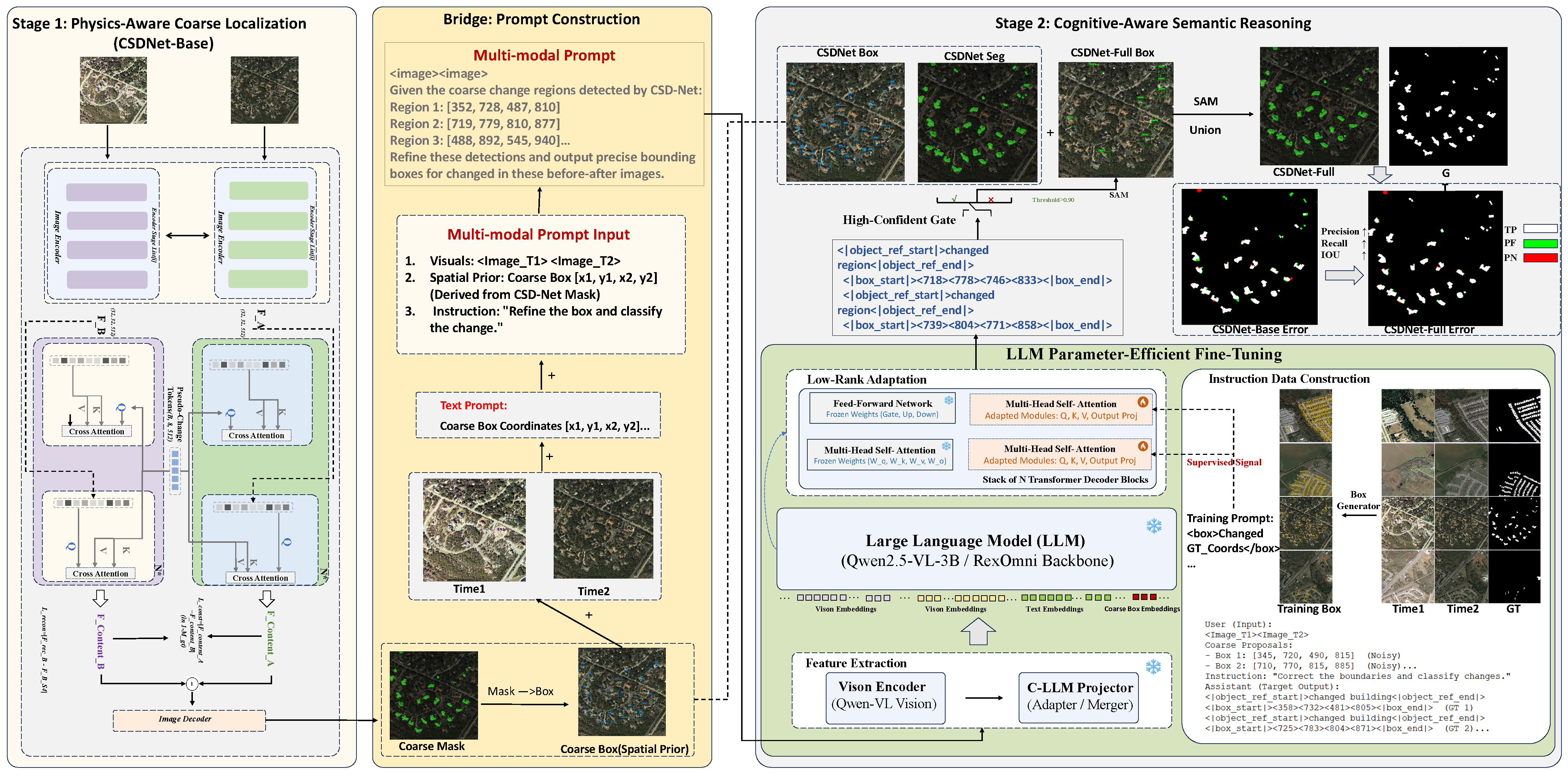
In this section, we elaborate on the proposed CSD-Net, a unified coarse-to-fine framework designed to address the twin challenges of pseudo-change interference and semantic ambiguity in RSCD. As illustrated in Figure 2, the framework operates in two progressive stages. The first stage, the style-aware base predictor, employs a content–style decoupling (CSD) mechanism to encourage separation between intrinsic content and extrinsic environmental style, generating a structural change prior. The second stage, the Cognitive-Aware Semantic Refiner, leverages an MLLM via spatially guided visual instruction tuning to refine coarse proposals on hard cases. Finally, an uncertainty-aware three-way softmax fusion integrates the base prior with the refined positive/negative evidence to produce robust final predictions.

3.1. Problem Formulation

Let $\mathcal{D}={\left\{(I^{t_1},I^{t_2},\mathbf{M})\right\}}_{i=1}^N$ denote a dataset of bi-temporal remote sensing images, where $I^{t_1},I^{t_2}\in {\mathbb{R}}^{H\times W\times 3}$ represent the pre-event and post-event images, and $\mathbf{M}\in {\{0,1\}}^{H\times W}$ is the ground-truth binary change map. The fundamental goal of RSCD is to model the posterior probability $P\left(\mathbf{M}\right|I^{t_1},I^{t_2})$.

3.1.1. Latent Content–Style Decomposition

Standard deep learning approaches typically map observations directly to predictions, i.e., $\mathcal{F}:(I^{t_1},I^{t_2})\to \mathbf{M}$. However, this assumes that feature disparity corresponds strictly to semantic change, which is often violated by pseudo-changes (e.g., phenological differences). To address this, we use a latent decomposition view in which the high-dimensional observation space $\mathcal{X}$ is represented by a latent manifold $\mathcal{Z}$ with a semantic content component ${\mathcal{Z}}_c$ and an environmental style component ${\mathcal{Z}}_s$. Formally, let $\Phi (·)$ be an encoder that maps an image I to its latent representation $\mathbf{z}$:

$$\mathbf{z}=\Phi \left(I\right)=[{\mathbf{z}}_c;{\mathbf{z}}_s],$$

(1)

where ${\mathbf{z}}_c$ captures the intrinsic geometry and category of ground objects, while ${\mathbf{z}}_s$ encapsulates extrinsic factors such as illumination and season.

In practice, this decomposition is encouraged through a dual-decoder structure with learnable pseudo-change tokens (detailed in Section 3.2). No direct style annotation is used. Instead, the content branch is supervised by the binary change mask, while reconstruction and temporal content-consistency losses constrain the decomposition to preserve information and reduce style-induced temporal variation.

The change prediction is formulated as a supervised binary classification on the content-dominant features, optimized via cross-entropy:

$$\begin{array}{cc}\hfill {\mathcal{L}}_{\mathrm{base}}=-\sum _{i,j}& [y_{i,j}log\sigma \left(f\left({\mathbf{z}}_c^{\Delta }(i,j)\right)\right)\hfill \\ \hfill & +(1-y_{i,j})log\left(1-\sigma \left(f\left({\mathbf{z}}_c^{\Delta }(i,j)\right)\right)\right)],\hfill \end{array}$$

(2)

where ${\mathbf{z}}_c^{\Delta }=|{\mathbf{z}}_c^{t_1}-{\mathbf{z}}_c^{t_2}|$ is the content-level difference, $f(·)$ is a convolutional decoder, $\sigma (·)$ is the sigmoid, and $y_{i,j}$ is the ground-truth label. This formulation naturally suppresses style-induced false alarms by marginalizing out ${\mathbf{z}}_s$.

3.1.2. Hierarchical Uncertainty-Aware Refinement

While the decomposition prior addresses pseudo-changes, pixel-level features ${\mathbf{z}}_c$ often lack the high-level reasoning required to resolve semantic ambiguities (e.g., distinguishing construction sites from barren land). We thus propose a two-stage hierarchical framework.

Let ${\mathbf{P}}_{\mathrm{base}}(i,j)=\sigma \left(f\left({\mathbf{z}}_c^{\Delta }(i,j)\right)\right)$ be the probability map from the content-based detector. We treat it as a dense base prior and introduce an MLLM as a cognitive semantic refiner. The MLLM is guided by spatial prompts $\mathcal{T}\left({\mathbf{P}}_{\mathrm{base}}\right)$ (coarse proposal boxes derived from uncertain regions) to refine each proposal by outputting a tighter box and a change/no-change decision with confidence. Positively refined boxes are then converted by SAM into pixel-accurate instance masks ${\mathbf{M}}_{\mathrm{sam}}$.

The final prediction is obtained via an uncertainty-aware three-way softmax fusion that combines the base prior with the refined positive/negative evidence from Stage 2.

Specifically, the MLLM refines each coarse proposal by predicting change or no-change. For change proposals, it additionally outputs a refined box to tighten the boundary. SAM then converts refined boxes into pixel-accurate instance masks that are aggregated into a positive evidence map ${\mathbf{M}}_{+}$ with a reliability map ${\mathbf{R}}_{+}$. For no-change proposals, since no refined coordinates are generated, we fall back to the original coarse proposal box to define the suppression region and construct the negative evidence map ${\mathbf{M}}_{-}$ with a reliability map ${\mathbf{R}}_{-}$.

Let $p={\mathbf{P}}_{\mathrm{base}}(i,j)$ denote the base probability at pixel $(i,j)$. We compute the normalized entropy as uncertainty:

$$u(i,j)={\displaystyle \frac{-plogp-(1-p)log(1-p)}{log2}}.$$

(3)

The fusion assigns three competing weights:

$$\begin{array}{cc}\hfill w_0(i,j)& =1,\hfill \\ \hfill w_{+}(i,j)& =exp(\kappa ·u(i,j))·{\mathbf{R}}_{+}(i,j),\hfill \\ \hfill w_{-}(i,j)& =exp(\kappa ·u(i,j))·{\mathbf{R}}_{-}(i,j),\hfill \end{array}$$

(4)

with $Z(i,j)=w_0(i,j)+w_{+}(i,j)+w_{-}(i,j)$. The fused score is

$$\mathbf{S}(i,j)={\displaystyle \frac{w_0(i,j){\mathbf{P}}_{\mathrm{base}}(i,j)+w_{+}(i,j){\mathbf{M}}_{+}(i,j)}{Z(i,j)}},$$

(5)

where $w_{-}(i,j)$ suppresses false positives by increasing the denominator $Z(i,j)$ in regions with reliable negative evidence. The final prediction is obtained by thresholding:

$${\mathbf{M}}_{\mathrm{final}}(i,j)=\mathbb{I}(\mathbf{S}(i,j)>\tau ).$$

(6)

The full construction of ${\mathbf{M}}_{+}$, ${\mathbf{M}}_{-}$, ${\mathbf{R}}_{+}$, ${\mathbf{R}}_{-}$ and the fusion details are provided in Section 3.4 and Section 3.5.

3.2. Style-Aware Content–Style Decoupling Network

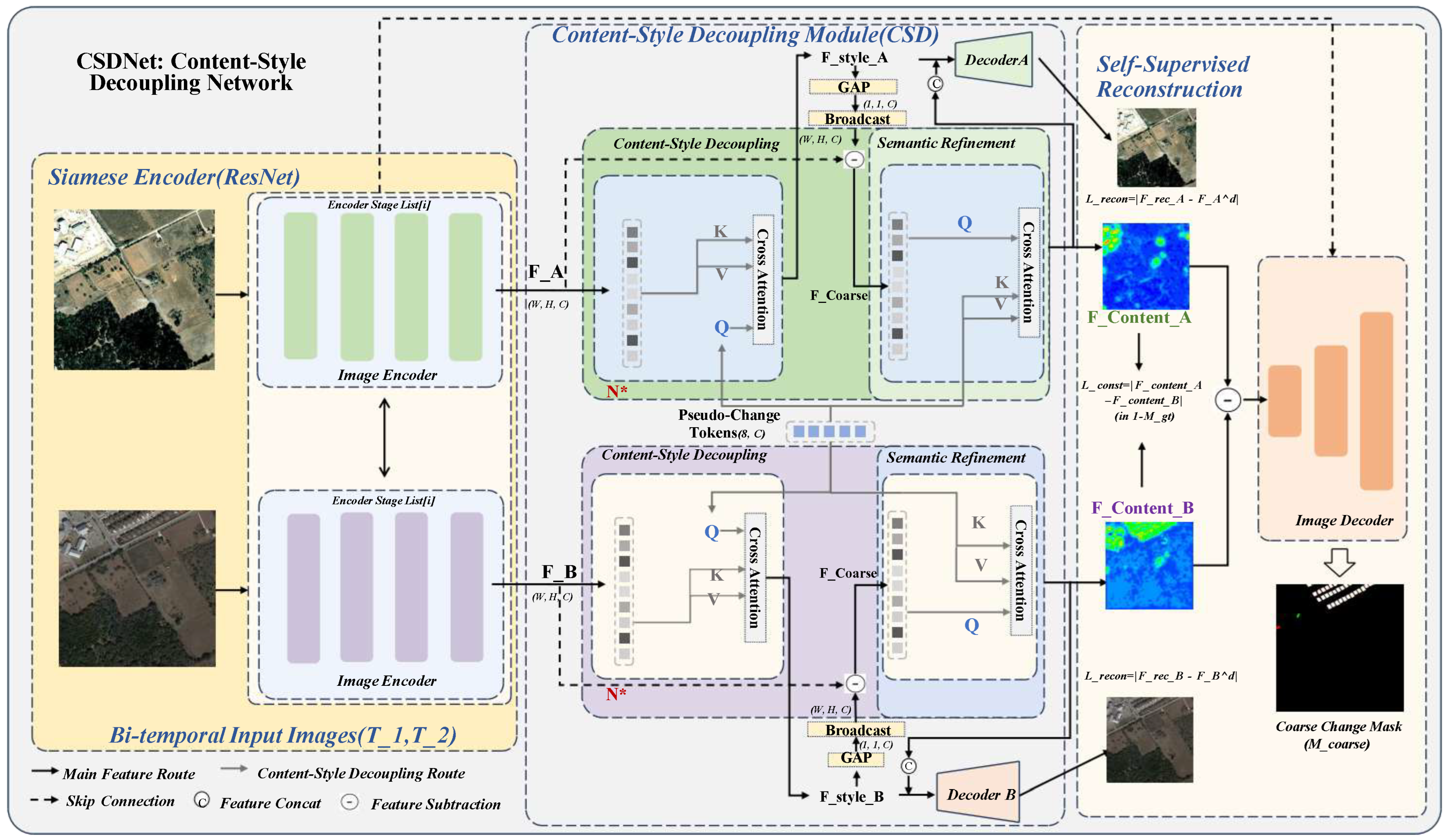
To build a strong pixel-level backbone that is robust to pseudo-changes, we adopt a Siamese deep network with a style-aware content–style decoupling (CSD) module. The detailed structure of the CSD module is shown in Figure 3. This subsection details the forward data flow and the associated loss functions, closely matching our implementation.

3.2.1. Siamese Feature Extraction and Perturbation

Given a bi-temporal pair $(I^{t_1},I^{t_2})\in {\mathbb{R}}^{H\times W\times 3}$, we first feed them into a weight-sharing ResNet-18 encoder:

$${\left\{F_l^{t_1}\right\}}_{l=1}^4,{\left\{F_l^{t_2}\right\}}_{l=1}^4=\Phi \left(I^{t_1}\right),\Phi \left(I^{t_2}\right),$$

(7)

where $F_l^t\in {\mathbb{R}}^{C_l\times H_l\times W_l}$ denotes the feature map at the l-th stage (from shallow to deep). To improve robustness against local noise and alignment errors, each stage is equipped with (i) a lightweight channel-wise Squeeze-and-Excitation (SE) block and (ii) a Perturbation Module (PM).

The PM takes the paired features $(F_l^{t_1},F_l^{t_2})$ and performs channel-level perturbation and exchange:

$${\tilde{F}}_l^{t_1},{\tilde{F}}_l^{t_2},D_l,A_l=\mathrm{PM}(F_l^{t_1},F_l^{t_2}),$$

(8)

where $D_l$ is a difference map and $A_l$ is an attention map. PM periodically swaps channels between the two inputs, applies a channel masking operation to emphasize discriminative channels, and then computes SE-style attention:

$$\begin{array}{cc}\hfill D_l& ={\tilde{F}}_l^{t_1}-{\tilde{F}}_l^{t_2},\hfill \end{array}$$

(9)

$$\begin{array}{cc}\hfill A_l& =\sigma \left(\mathrm{MLP}\left(\mathrm{GAP}\left(D_l\right)\right)+\mathrm{MLP}\left(D_l\right)\right),\hfill \end{array}$$

(10)

where $\mathrm{GAP}(·)$ is global average pooling, MLP is a two-layer $1\times 1$ convolutional network, and $\sigma (·)$ is the sigmoid. The final enhanced features are

$${\widehat{F}}_l^{t_1}=F_l^{t_1}+A_l\odot F_l^{t_1},{\widehat{F}}_l^{t_2}=F_l^{t_2}+A_l\odot F_l^{t_2},$$

(11)

which are fed into deeper stages and the multi-scale fusion head.

3.2.2. Transformer-Based Content–Style Decoupling

The core of CSD-Net is a structured decomposition of content-dominant and style-dominant components at a high-level encoder stage. Let $F_d^{t_1},F_d^{t_2}\in {\mathbb{R}}^{C_d\times H_d\times W_d}$ denote the selected deep features (in our implementation, $C_d=512$ and $H_d=W_d=32$ for $256\times 256$ inputs). We introduce a set of learnable pseudo-change tokens $P\in {\mathbb{R}}^{K\times C_d}$ (with $K=8$) that serve as a compact style bank shared across the dataset. This setting is consistent with Figure 3 and adds only $8\times 512=4096$ token parameters.

For each time $t\in \{t_1,t_2\}$, we first flatten the feature map:

$$X^t=\mathrm{Flatten}\left(F_d^t\right)\in {\mathbb{R}}^{N\times C_d},N=H_d{W}_d,$$

(12)

and broadcast the pseudo-tokens to match the batch size:

$$P_b=\mathrm{Repeat}(P,B)\in {\mathbb{R}}^{B\times K\times C_d}.$$

(13)

Then a shared transformer decoder with L layers (we use $L=2$, $d_{\mathrm{model}}=C_d$, 8 heads) is applied in a cascade manner: (i) subtraction for feature-level style compensation followed by (ii) cross-attention for residual refinement.

Style aggregation stream (estimate global bias). Conversely, pseudo-tokens query the image features to aggregate style information:

$$S_{\mathrm{tokens}}^t=\mathrm{Dec}\left(\mathrm{tgt}=P_b,\mathrm{memory}=X^t\right)\in {\mathbb{R}}^{B\times K\times C_d}.$$

(14)

Redefining “style” as global environmental priors. In remote sensing, a large portion of pseudo-changes stems from global radiometric variations—seasonal phenology, illumination differences, and atmospheric scattering/haze—that are often spatially coherent at the image level. We therefore deliberately define the “style” branch as Global Environmental Priors rather than generic appearance.

Pseudo-change tokens as learnable environmental prototypes. Accordingly, the pseudo-change tokens P are not meant to memorize object textures; instead, they serve as learnable environmental prototypes that summarize common imaging-condition distributions in the dataset (e.g., “hazy”, “snowy”, “over-exposed”). Through cross-attention, these prototypes absorb scene-level radiometric cues from $X^t$ into $S_{\mathrm{tokens}}^t$.

Broadcasting as a global style constraint. We then average over the token dimension and broadcast the result to the spatial resolution:

$$S_{\mathrm{map}}^t=\mathrm{Broadcast}\left(\mathrm{Mean}(S_{\mathrm{tokens}}^t,\dim =1)\right)\in {\mathbb{R}}^{C_d\times H_d\times W_d}.$$

(15)

This broadcast operation constrains $S_{\mathrm{map}}^t$ to be spatially invariant, i.e., $S_{\mathrm{map}}^t(i,j)$ is identical for all positions $(i,j)$. This design makes it difficult for the style branch to represent local object geometry such as the shape of a building because such information requires spatial variation. We therefore interpret $S_{\mathrm{map}}^t$ as a feature-level proxy for dominant image-level style factors, such as season or overall illumination, rather than as a complete model of all radiometric effects. Under this constraint, the content branch $C^t$ is encouraged to retain intrinsic geometric semantics, while the style branch summarizes image-level environmental priors.

Interpretation of subtraction as feature-level bias compensation. We further provide a formal interpretation for the subtraction operation used in the content stream. With an additive environmental bias approximation, we model the observed deep feature at time t as a superposition of intrinsic semantic content and an extrinsic global style shift:

$$X^t(i,j)\approx C^t(i,j)+S_{\mathrm{bias}}^t,$$

(16)

where $S_{\mathrm{bias}}^t$ is a spatially constant bias vector approximating image-level radiometric variations (e.g., seasonal spectral shift, illumination tone, and atmospheric scattering). Since the broadcast operation enforces $S_{\mathrm{map}}^t$ to be spatially invariant, $S_{\mathrm{map}}^t$ can be viewed as a feature-space estimator of this dominant global bias. Consequently, the subtraction $F_{\mathrm{coarse}}=F_{\mathrm{input}}-S_{\mathrm{map}}^t$ acts as a feature-level compensation step for the estimated environmental shift. This interpretation is intentionally limited to dominant global style factors; strongly local shadows, partial haze, or non-uniform sensor artifacts may require additional spatially adaptive modeling.

Step-1: Subtraction (global style compensation). We compensate the deep feature by subtracting the broadcast style map:

$$F_{\mathrm{coarse}}^t=F_d^t-S_{\mathrm{map}}^t\in {\mathbb{R}}^{C_d\times H_d\times W_d}.$$

(17)

This subtraction is dimension-consistent (e.g., $(B,H_d,W_d,C_d)-(B,H_d,W_d,C_d)$) and can be interpreted as feature-level compensation for spatially invariant environmental bias.

Step-2: Content refinement stream (residual semantic repair). We then flatten $F_{\mathrm{coarse}}^t$ to obtain $X_{\mathrm{coarse}}^t=\mathrm{Flatten}\left(F_{\mathrm{coarse}}^t\right)$ and let it query the pseudo-tokens to refine remaining local nonlinear residuals:

$$Z_c^t=\mathrm{Dec}\left(\mathrm{tgt}=X_{\mathrm{coarse}}^t,\mathrm{memory}=P_b\right)\in {\mathbb{R}}^{N\times C_d},$$

(18)

which is reshaped back to a spatial map $C^t\in {\mathbb{R}}^{C_d\times H_d\times W_d}$ as the refined content representation. This “subtraction → refinement” hierarchy yields a coarse-to-fine interpretation: global style compensation first, then attention-based residual refinement.

3.2.3. Reconstruction and Consistency Constraints

To encourage the decomposition to remain information-complete, we reconstruct the original features from the decomposed components via a lightweight reconstructor $\mathcal{R}$:

$${\widehat{F}}_d^t=\mathcal{R}\left(\mathrm{Concat}(C^t,S_{\mathrm{map}}^t)\right)\in {\mathbb{R}}^{C_d\times H_d\times W_d},$$

(19)

where $\mathcal{R}$ consists of a $1\times 1$ convolution (reducing $2C_d\to C_d$) followed by a $3\times 3$ convolution with batch normalization and ReLU.

The reconstruction loss is defined as

$${\mathcal{L}}_{\mathrm{recon}}=\sum _{t\in \{t_1,t_2\}}\parallel {\widehat{F}}_d^t-F_d^t{\parallel }_1.$$

(20)

This loss acts as a soft “information conservation” constraint, encouraging $C^t$ and $S_{\mathrm{map}}^t$ to form a complementary decomposition.

To explicitly suppress pseudo-changes, we further enforce temporal consistency of content features over unchanged regions. Let $\mathbf{M}\in {\{0,1\}}^{H\times W}$ be the ground-truth binary change map (1 for change, 0 for no-change), and let ${\Omega }_{\mathrm{uc}}$ be the set of spatial positions that are downsampled from unchanged pixels (we compute an unchanged mask at resolution $H_d\times W_d$ by nearest-neighbor downsampling and inversion of $\mathbf{M}$). The content consistency loss is

$${\mathcal{L}}_{\mathrm{const}}={\displaystyle \frac{1}{|{\Omega }_{\mathrm{uc}}|}}\sum _{(i,j)\in {\Omega }_{\mathrm{uc}}}\parallel C^{t_1}(i,j)-C^{t_2}(i,j){\parallel }_1.$$

(21)

This loss explicitly pushes the content features of unchanged regions to be invariant across time, forcing illumination and seasonal differences to be absorbed by the style branch.

3.2.4. Multi-Scale Fusion and Supervision

After decoupling, the content-dominant features $C^{t_1}$ and $C^{t_2}$ are used to compute a semantic change descriptor:

$$D_{\mathrm{cont}}=|C^{t_1}-C^{t_2}|\in {\mathbb{R}}^{C_d\times H_d\times W_d},$$

(22)

which is propagated through a bi-directional feature pyramid network (Bi-FPN) together with lower-level difference and attention maps $\{D_l,A_l\}$ to generate multi-scale features ${\left\{F_l^{\Delta }\right\}}_{l=1}^4$.

Our decode head takes these fused features and predicts:

• A main change probability map ${\mathbf{P}}_{\mathrm{main}}\in {[0,1]}^{H\times W}$;
• An auxiliary attention-difference map ${\mathbf{P}}_{\mathrm{att}}\in {[0,1]}^{H_a\times W_a}$;
• A distance-based contrastive map ${\mathbf{P}}_{\mathrm{dist}}\in {[0,1]}^{H_a\times W_a}$.

The overall supervision for the base network is a weighted combination of three terms:

$${\mathcal{L}}_{\mathrm{base}}={\mathcal{L}}_{\mathrm{ce}}^{\mathrm{main}}+{\mathcal{L}}_{\mathrm{ce}}^{\mathrm{att}}+{\mathcal{L}}_{\mathrm{ctr}},$$

(23)

where ${\mathcal{L}}_{\mathrm{ce}}^{\mathrm{main}}$ and ${\mathcal{L}}_{\mathrm{ce}}^{\mathrm{att}}$ are standard pixel-wise cross-entropy losses computed on the main and auxiliary logits, respectively. The contrastive loss ${\mathcal{L}}_{\mathrm{ctr}}$ is a margin-based formulation operating on the distance map:

$${\mathcal{L}}_{\mathrm{ctr}}={\displaystyle \frac{1}{N}}{\displaystyle \sum _{i=1}^N}\left[(1-y_i)p_i^2+y_i{\left(max(m-p_i,0)\right)}^2\right],$$

(24)

where $p_i$ is the predicted distance at pixel i, $y_i\in \{0,1\}$ is the corresponding label (change vs. no-change), and $m=1$ is the margin.

Finally, the decoupling-related losses are integrated with small weights:

$${\mathcal{L}}_{\mathrm{total}}={\mathcal{L}}_{\mathrm{base}}+{\lambda }_{\mathrm{recon}}{\mathcal{L}}_{\mathrm{recon}}+{\lambda }_{\mathrm{const}}{\mathcal{L}}_{\mathrm{const}},$$

(25)

where we set ${\lambda }_{\mathrm{recon}}=1\times {10}^{-4}$ and ${\lambda }_{\mathrm{const}}=2\times {10}^{-4}$ in all experiments. The final sigmoid output of the main head is used as the base prior ${\mathbf{P}}_{\mathrm{base}}$ for the MLLM+SAM refinement stage.

3.3. Spatial-Guided Visual Instruction Tuning

While CSD-Net provides reliable pixel-wise localization, it may still struggle in semantically ambiguous cases (e.g., distinguishing construction sites from barren land). To inject high-level semantic reasoning while retaining efficiency, we extend it to CSD-Net⁺ by attaching an optional MLLM through spatially guided visual instruction tuning. Importantly, the MLLM is not merely a binary verifier; instead, it acts as a coarse-to-fine semantic refiner that takes a coarse proposal box from the base model as a spatial prompt and generates a refined box with an associated change decision. In our implementation, we adopt a Qwen2.5-3B multimodal model and initialize it from the Rex-Omni checkpoint [13] and then perform supervised fine-tuning (SFT) with LoRA. For clarity, we denote the resulting refiner as Rex-Omni-R.

Why not directly use the MLLM for change detection? A natural question is why we adopt a box-refine-then-SAM pipeline rather than having the MLLM directly output change masks. There are three reasons. (i) Granularity gap: Current MLLMs with grounding capability (e.g., GeoChat [10] and Rex-Omni [13]) output box-level or point-level localization—not pixel-accurate masks required for mapping-grade CD. Even with next-point-prediction paradigms, dense mask generation remains unreliable for fine boundaries. (ii) Generation quality: We find that MLLMs fine-tuned on CD data can produce plausible-looking change descriptions but exhibit unstable box coordinates under distribution shift conditions (e.g., novel building styles), whereas a specialized detector (CSD-Net Base) provides a reliable, calibrated prior. (iii) Efficiency: Running an MLLM densely over the full image (sliding window or full-resolution encoding) is computationally prohibitive for practical deployment. Our spatially guided strategy restricts MLLM queries to a small set of uncertain proposals (≪image area), making Stage 2 tractable. The refined boxes are then passed to SAM for boundary-accurate mask generation, exploiting SAM’s strong zero-shot segmentation capability while avoiding its known limitations in semantic disambiguation.

3.3.1. Bi-Temporal Visual Token Construction

Rex-Omni-R builds upon a Qwen-style multimodal architecture (vision transformer encoder + causal LLM backbone). Given the bi-temporal images $I^{t_1},I^{t_2}$, we first run the shared ViT encoder and a multi-scale projector (C-Abstractor) to obtain compact visual embeddings:

$$V^{t_1}=f_{\mathrm{vis}}\left(I^{t_1}\right)\in {\mathbb{R}}^{N_1\times d},V^{t_2}=f_{\mathrm{vis}}\left(I^{t_2}\right)\in {\mathbb{R}}^{N_2\times d},$$

(26)

where d is the hidden dimension of the LLM (e.g., $d=4096$), and $N_1,N_2$ are the numbers of merged patch tokens after dynamic resolution adjustment and $2\times 2$ patch merging.

The two sets of visual tokens are serialized into the language model input using reserved delimiters:

$$\begin{array}{cc}\hfill X_{\mathrm{vis}}=& [<|\mathtt{vision}\text{\_}\mathtt{start}|>,V^{t_1},<\left|\mathtt{vision}\text{\_}\mathtt{end}\right|>,\hfill \\ \hfill & <\left|\mathtt{vision}\text{\_}\mathtt{start}\right|>,V^{t_2},<\left|\mathtt{vision}\text{\_}\mathtt{end}\right|>].\hfill \end{array}$$

(27)

These tokens are concatenated with system and user prompts to form the full input sequence:

$$\begin{array}{cc}\hfill X=& [<|\mathtt{im}\text{\_}\mathtt{start}|>\mathrm{system},\mathrm{SYS},<|\mathtt{im}\text{\_}\mathtt{end}|>,\hfill \\ \hfill & <\left|\mathtt{im}\text{\_}\mathtt{start}\right|>\mathrm{user},X_{\mathrm{vis}},\mathrm{INST},<\left|\mathtt{im}\text{\_}\mathtt{end}\right|>,\hfill \\ \hfill & <\left|\mathtt{im}\text{\_}\mathtt{start}\right|>\mathrm{assistant}],\hfill \end{array}$$

(28)

where SYS denotes the system prompt and INST provides the task instruction conditioned on a coarse proposal box, e.g., “Given the coarse proposal, refine the box boundary and answer change or no-change.”.

3.3.2. Coarse Proposal Encoding and Refined-Box Generation

In CSD-Net⁺, we use the MLLM as a semantic refiner rather than a free-form detector. The base model first generates a set of coarse proposal boxes ${\mathcal{B}}_{\mathrm{coarse}}$ from uncertain regions. For each proposal $b_k^{\left(c\right)}\in {\mathcal{B}}_{\mathrm{coarse}}$, Rex-Omni-R takes the bi-temporal images and the coarse box as a spatial prompt and produces (i) a refined box ${\widehat{b}}_k^{\left(r\right)}$ with tighter boundaries and (ii) a binary decision $y_k\in \{\mathtt{change},\mathtt{no}\text{-}\mathtt{change}\}$ with confidence.

Coarse box encoding (input). To represent a coarse proposal in the prompt, we define

$$b^{\left(c\right)}=(x_{min},y_{min},x_{max},y_{max}).$$

We then normalize and quantize each coordinate into an integer in $[0,999]$:

$$\begin{array}{cc}\hfill c_x& =⌊{\displaystyle \frac{x}{W}}·999⌋,c_y=⌊{\displaystyle \frac{y}{H}}·999⌋,\hfill \end{array}$$

(29)

and serialize them with reserved delimiters as

$$<\left|\mathtt{box}\text{\_}\mathtt{start}\right|>c_y^{min}{c}_x^{min}{c}_y^{max}{c}_x^{max}<\left|\mathtt{box}\text{\_}\mathtt{end}\right|>.$$

These coordinate tokens serve as a spatial prompt that constrains the MLLM to focus on the coarse region.

Refined-box + label output (assistant). The supervised target output contains (i) refined coordinate tokens and (ii) a change label. For a positive proposal, the model outputs

$$\begin{array}{cc}\hfill Y_{\mathrm{tgt}}=& [<|\mathtt{box}\text{\_}\mathtt{start}|>{\widehat{c}}_y^{min}{\widehat{c}}_x^{min}{\widehat{c}}_y^{max}{\widehat{c}}_x^{max}<\left|\mathtt{box}\text{\_}\mathtt{end}\right|>\hfill \\ \hfill & ;\mathtt{change}],\hfill \end{array}$$

(30)

while for a negative proposal it outputs $\left[\mathtt{no}\text{-}\mathtt{change}\right]$ (i.e., no refined box is emitted). During inference, we compute a confidence score $q_k$ from the token-level probability of the predicted label and decode ${\widehat{b}}_k^{\left(r\right)}$ from the generated coordinate tokens.

Training objective (SFT with box regression supervision). We fine-tune Rex-Omni-R to both classify and regress precise boundaries. Let ${\mathcal{L}}_{\mathrm{CE}}$ denote the standard causal language modeling loss on the assistant tokens (including label and coordinate tokens). For positive proposals, we additionally impose a GIoU-based box alignment loss between the decoded refined box ${\widehat{b}}^{\left(r\right)}$ and the ground-truth box $b^{\star }$:

$${\mathcal{L}}_{\mathrm{box}}=1-\mathrm{GIoU}({\widehat{b}}^{\left(r\right)},b^{\star }).$$

(31)

The total SFT objective is

$${\mathcal{L}}_{\mathrm{SFT}}={\mathcal{L}}_{\mathrm{CE}}+{\lambda }_{\mathrm{box}}{\mathcal{L}}_{\mathrm{box}},$$

(32)

where ${\lambda }_{\mathrm{box}}$ balances generation fidelity and boundary accuracy. For negative proposals ($y=\mathtt{no}\text{-}\mathtt{change}$), ${\mathcal{L}}_{\mathrm{box}}$ is omitted.

Summary of the Fusion Strategy

Base prior: CSD-Net (Base) yields a dense probability map ${\mathbf{P}}_{\mathtt{base}}$. Positive evidence: The MLLM refines coarse proposals and predicts change; SAM converts refined boxes into tight instance masks ${\mathbf{M}}_{+}$ with reliability ${\mathbf{R}}_{+}$, enabling false negative recovery. Negative evidence: The MLLM predicts no-change for a coarse proposal; since no refined coordinates are generated, the coarse box region forms ${\mathbf{M}}_{-}$ with reliability ${\mathbf{R}}_{-}$, suppressing false positives by increasing the fusion denominator. Uncertainty-aware three-way fusion: Equation (48) amplifies Stage 2 evidence in uncertain regions while preserving base predictions in confident regions.

3.3.3. LoRA-Based Parameter-Efficient Tuning

Fine-tuning the full Rex-Omni model is computationally expensive. We therefore adopt Low-Rank Adaptation (LoRA) to adjust only a small subset of parameters while freezing the majority of the backbone.

Let $W_0\in {\mathbb{R}}^{d_{\mathrm{out}}\times d_{\mathrm{in}}}$ denote a pretrained weight matrix in a linear layer of the LLM. LoRA introduces two low-rank matrices $A\in {\mathbb{R}}^{r\times d_{\mathrm{in}}}$ and $B\in {\mathbb{R}}^{d_{\mathrm{out}}\times r}$, and re-parameterizes the effective weight as

$$W=W_0+{\displaystyle \frac{\alpha }{r}}BA,$$

(33)

where r is the rank and $\alpha$ is a scaling factor. We follow the configuration

$$r=64,\alpha =128,\mathrm{dropout}=0.05.$$

(34)

We apply LoRA to the following linear projections in all transformer blocks of the LLM:

• Multi-Head Attention: query, key, value, and output projections (q_proj, k_proj, v_proj, o_proj);
• Feed-Forward Network: gate, up, and down projections (gate_proj, up_proj, down_proj).

The ViT-based vision encoder and all other backbone parameters are kept frozen. This yields a parameter-efficient semantic refiner, Rex-Omni-R, with only about $2\%$ of the total parameters being trainable.

3.3.4. Instruction Tuning Objective

Rex-Omni-R is trained with a standard causal language modeling objective. Let $x_{1:L}$ be the tokenized input–output sequence produced by the chat template (system + user + assistant) with bi-temporal visual tokens inserted. We mask out all tokens that belong to the system and user roles, as well as the visual tokens, so that only the assistant’s reply contributes to the loss.

Formally, the token-level generation loss is

$${\mathcal{L}}_{\mathrm{CE}}=-{\displaystyle \sum _{t=1}^L}{m}_{t}log{p}_{\theta }(x_t\mid x_{<t},I^{t_1},I^{t_2}),$$

(35)

where $m_t=1$ if $x_t$ belongs to the assistant’s answer (i.e., the refined coordinate tokens and the label), and $m_t=0$ otherwise. The final SFT objective adds the IoU/GIoU box alignment term for positive proposals, as in Equation (32).

3.3.5. Candidate Box Generation

To generate coarse proposal boxes ${\mathcal{B}}_{\mathrm{coarse}}$ for refinement, we first identify uncertain regions from the base probability map. Specifically, we compute the normalized entropy $u(i,j)$ (Equation (43)) and threshold it:

$${\mathbf{M}}_{\mathrm{uncertain}}=\mathbb{I}(u(i,j)>u_0),$$

(36)

where $u_0=0.5$ is the uncertainty threshold. To avoid querying the MLLM on noisy isolated pixels, we apply a $3\times 3$ morphological closing operation, run connected component analysis on ${\mathbf{M}}_{\mathrm{uncertain}}$, and compute the axis-aligned bounding box for each connected region. Small regions (area $<100$ pixels) are filtered out. Each remaining box is enlarged by 10% on each side and clipped to the image boundary so that contextual cues around the uncertain region are retained. If more than $N_{max}=20$ components are found in one image, we keep the top-$N_{max}$ boxes ranked by average entropy. This yields ${\mathcal{B}}_{\mathrm{coarse}}=\{b_1^{\left(c\right)},b_2^{\left(c\right)},\dots ,b_K^{\left(c\right)}\}$.

Training data construction. During training of Rex-Omni-R, we construct positive and negative refinement instructions from the training images only. Positive samples are obtained by converting ground-truth change masks into connected components and bounding boxes. For each positive component, we create a coarse proposal by either (i) jittering the GT box with random translation and scale within $\pm 10\%$ of the box size or (ii) matching a base-model uncertain proposal whose IoU with the GT box is larger than 0.3. The assistant target is change together with the GT-aligned refined box.

Negative samples are constructed from two sources: (i) random boxes sampled from no-change regions with IoU $<0.05$ to all GT change boxes and (ii) hard negatives mined from base-model false-positive or high-uncertainty no-change regions. For each image, we keep at most 10 positive proposals and 10 negative proposals to maintain a balanced instruction set. If an image contains fewer positives or negatives, all available samples are used. Negative targets output only the no-change label without refined coordinates. This protocol clarifies the false-positive and false-negative sampling strategy used to train the refiner.

3.3.6. Inference: Box Refinement and Evidence Construction

At inference time, CSD-Net (Base) produces a probability map ${\mathbf{P}}_{\mathrm{base}}$ and generates coarse proposal boxes ${\mathcal{B}}_{\mathrm{coarse}}$ using the entropy-based procedure above. No ground-truth masks are used at inference. For each proposal $b_k^{\left(c\right)}\in {\mathcal{B}}_{\mathrm{coarse}}$, we query Rex-Omni-R with the bi-temporal images and the coarse box tokens and obtain a decision $y_k\in \{\mathtt{change},\mathtt{no}\text{-}\mathtt{change}\}$ and a confidence score $q_k$ computed as the softmax probability of the generated label token. If $y_k=\mathtt{change}$, Rex-Omni-R also outputs a refined box ${\widehat{b}}_k^{\left(r\right)}$; otherwise, no refined coordinates are emitted. In practice, the top-20 entropy-ranked proposals are queried per image, and proposals below the confidence threshold $\tau =0.5$ fall back to the base prediction in the final fusion.

For proposals refined as change, we apply SAM with the refined box ${\widehat{b}}_k^{\left(r\right)}$ as the box prompt to obtain a pixel-accurate instance mask ${\mathbf{M}}_{\mathrm{sam}}^{\left(k\right)}$ and a mask quality score $s_k$ (Section 3.4). For proposals predicted as no-change, since no refined coordinates are emitted, we treat the coarse proposal box region $b_k^{\left(c\right)}$ as negative evidence. These outputs are aggregated into the evidence maps ${\mathbf{M}}_{+}$, ${\mathbf{M}}_{-}$ and the reliability maps ${\mathbf{R}}_{+}$, ${\mathbf{R}}_{-}$, which are fused with ${\mathbf{P}}_{\mathrm{base}}$ using the uncertainty-aware three-way softmax fusion in Section 3.5.

3.4. SAM-Based Instance Mask Refinement

While the MLLM provides semantic guidance, bounding boxes are inherently rectangular and cannot capture precise object boundaries. To bridge this granularity gap, we employ the Segment Anything Model (SAM) [14] to convert refined boxes generated by Rex-Omni-R into pixel-accurate instance masks with sharp boundaries.

3.4.1. Box-Prompted SAM Segmentation

For each positively refined proposal (i.e., $y_k=\mathtt{change}$), we use the refined box ${\widehat{b}}_k^{\left(r\right)}$ generated by Rex-Omni-R as the box prompt for SAM on the post-event image $I^{t_2}$:

$${\mathbf{M}}_{\mathrm{sam}}^{\left(k\right)},s_k=\mathrm{SAM}(I^{t_2},{\widehat{b}}_k^{\left(r\right)}),$$

(37)

where ${\mathbf{M}}_{\mathrm{sam}}^{\left(k\right)}\in {\{0,1\}}^{H\times W}$ is the binary instance mask and $s_k\in [0,1]$ is SAM’s predicted IoU score indicating mask quality. The reliability of each SAM-refined mask is computed as

$$r_k=q_k·s_k,$$

(38)

where $q_k$ is Rex-Omni-R’s confidence for the refined proposal ${\widehat{b}}_k^{\left(r\right)}$. This product ensures that both semantic correctness (from Rex-Omni-R) and boundary quality (from SAM) contribute to the final reliability.

For proposals refined as no-change, we set $r_k=q_k$ since no SAM mask quality is available.

3.4.2. Positive and Negative Evidence Maps

We aggregate the SAM-refined masks into a positive evidence map ${\mathbf{M}}_{+}$ that indicates regions refined as changed:

$${\mathbf{M}}_{+}=\bigcup _{k:y_k=\mathtt{change}}{\mathbf{M}}_{\mathrm{sam}}^{\left(k\right)},$$

(39)

with a corresponding reliability map:

$${\mathbf{R}}_{+}(i,j)=\underset{k:(i,j)\in {\mathbf{M}}_{\mathrm{sam}}^{\left(k\right)}}{max}{r}_k.$$

(40)

Similarly, for proposals predicted as no-change (i.e., $y_k=\mathtt{no}\text{-}\mathtt{change}$), since no refined coordinates are generated, we utilize the original coarse proposal box $b_k^{\left(c\right)}$ to define the suppression region. We construct the negative evidence map ${\mathbf{M}}_{-}$ as

$${\mathbf{M}}_{-}=\bigcup _{k:y_k=\mathtt{no}\text{-}\mathtt{change}}\mathbb{I}((i,j)\in b_k^{\left(c\right)}),$$

(41)

where $b_k^{\left(c\right)}$ denotes the spatial extent of the input coarse proposal, with reliability

$${\mathbf{R}}_{-}(i,j)=\underset{k:(i,j)\in b_k^{\left(c\right)}}{max}{r}_k.$$

(42)

The positive evidence ${\mathbf{M}}_{+}$ enables recovery of false negatives (missed changes), while the negative evidence ${\mathbf{M}}_{-}$ enables suppression of false positives (incorrectly detected changes).

3.5. Uncertainty-Aware Three-Way Softmax Fusion

To integrate the base prior ${\mathbf{P}}_{\mathrm{base}}$ with the positive and negative evidence from Stage 2, we propose a three-way softmax fusion mechanism that dynamically adjusts weights based on pixel-wise uncertainty.

3.5.1. Pixel-Wise Uncertainty Estimation

Let $p={\mathbf{P}}_{\mathrm{base}}(i,j)$ denote the base model’s change probability at pixel $(i,j)$. We compute the normalized entropy as the uncertainty measure:

$$u(i,j)={\displaystyle \frac{-plogp-(1-p)log(1-p)}{log2}},$$

(43)

where $u(i,j)\in [0,1]$ is low when the base model is confident ($p\approx 0$ or $p\approx 1$) and peaks at 1 when $p=0.5$ (maximum ambiguity).

3.5.2. Three-Way Softmax Fusion

We define three competing contributions at each pixel: the base prediction, the positive evidence, and the negative evidence. The overall procedure is summarized in Algorithm 1. The unnormalized weights are

$$\begin{array}{cc}\hfill w_0(i,j)& =1,\hfill \end{array}$$

(44)

$$\begin{array}{cc}\hfill w_{+}(i,j)& =exp(\kappa ·u(i,j))·{\mathbf{R}}_{+}(i,j),\hfill \end{array}$$

(45)

$$\begin{array}{cc}\hfill w_{-}(i,j)& =exp(\kappa ·u(i,j))·{\mathbf{R}}_{-}(i,j),\hfill \end{array}$$

(46)

where $\kappa =5$ controls how strongly uncertainty amplifies the Stage 2 evidence. The normalization factor is

$$Z(i,j)=w_0(i,j)+w_{+}(i,j)+w_{-}(i,j).$$

(47)

The fused score map is computed as

$$\mathbf{S}(i,j)={\displaystyle \frac{w_0(i,j){\mathbf{P}}_{\mathrm{base}}(i,j)+w_{+}(i,j){\mathbf{M}}_{+}(i,j)}{w_0(i,j)+w_{+}(i,j)+w_{-}(i,j)}}.$$

(48)

The final binary change mask is obtained by thresholding:

$${\mathbf{M}}_{\mathrm{final}}(i,j)=\mathbb{I}(\mathbf{S}(i,j)>\tau ),$$

(49)

where $\tau =0.5$ is the default threshold.

Algorithm 1 Uncertainty-aware three-way softmax fusion with MLLM refinement and SAM refinement

Require: Pre-event image $I^{t_1}$, post-event image $I^{t_2}$;   1: Base probability map ${\mathbf{P}}_{\mathrm{base}}\in {[0,1]}^{H\times W}$;   2: Coarse proposal boxes ${\mathcal{B}}_{\mathrm{coarse}}$ from uncertain regions;   3: Hyperparameter $\kappa$; threshold $\tau$.  Ensure: Final change mask ${\mathbf{M}}_{\mathrm{final}}\in {\{0,1\}}^{H\times W}$.   4: Step 1: Compute base uncertainty   5: $u\leftarrow {\displaystyle \frac{-{\mathbf{P}}_{\mathrm{base}}log{\mathbf{P}}_{\mathrm{base}}-(1-{\mathbf{P}}_{\mathrm{base}})log(1-{\mathbf{P}}_{\mathrm{base}})}{log2}}$   6: Step 2: Initialize evidence maps   7: ${\mathbf{M}}_{+}\leftarrow \mathbf{0}$, ${\mathbf{R}}_{+}\leftarrow \mathbf{0}$, ${\mathbf{M}}_{-}\leftarrow \mathbf{0}$, ${\mathbf{R}}_{-}\leftarrow \mathbf{0}$   8: Step 3: MLLM refinement and evidence construction   9: for each coarse box $b_k^{\left(c\right)}$ in ${\mathcal{B}}_{\mathrm{coarse}}$ do 10:       $({\widehat{b}}_k^{\left(r\right)},y_k,q_k)\leftarrow \mathrm{Rex}\text{-}\mathrm{Omni}\text{-}\mathrm{R}(I^{t_1},I^{t_2},b_k^{\left(c\right)})$       ▹$y_k\in \{\mathtt{change},\mathtt{no}\text{-}\mathtt{change}\}$ 11:       if $y_k=\mathtt{change}$ then 12:          $({\mathbf{M}}_{\mathrm{sam}}^{\left(k\right)},s_k)\leftarrow \mathrm{SAM}(I^{t_2},{\widehat{b}}_k^{\left(r\right)})$ 13:          $r_k\leftarrow q_k·s_k$ 14:          ${\mathbf{M}}_{+}\leftarrow {\mathbf{M}}_{+}\cup {\mathbf{M}}_{\mathrm{sam}}^{\left(k\right)}$ 15:          for each pixel $(i,j)$ such that ${\mathbf{M}}_{\mathrm{sam}}^{\left(k\right)}(i,j)=1$ do 16:                ${\mathbf{R}}_{+}(i,j)\leftarrow max({\mathbf{R}}_{+}(i,j),r_k)$ 17:          end for 18:       else 19:          $r_k\leftarrow q_k$ 20:          Set ${\mathbf{M}}_{-}(i,j)\leftarrow 1$ for all $(i,j)\in b_k^{\left(c\right)}$ 21:          for each pixel $(i,j)$ such that $(i,j)\in b_k^{\left(c\right)}$ do 22:                ${\mathbf{R}}_{-}(i,j)\leftarrow max({\mathbf{R}}_{-}(i,j),r_k)$ 23:          end for 24:       end if 25: end for 26: Step 4: Three-way softmax fusion 27: $w_0\leftarrow \mathbf{1}$                             ▹ all-ones map 28: $w_{+}\leftarrow exp(\kappa ·u)\odot {\mathbf{R}}_{+}$ 29: $w_{-}\leftarrow exp(\kappa ·u)\odot {\mathbf{R}}_{-}$ 30: $Z\leftarrow w_0+w_{+}+w_{-}$ 31: $\mathbf{S}\leftarrow \left(w_0\odot {\mathbf{P}}_{\mathrm{base}}+w_{+}\odot {\mathbf{M}}_{+}\right)\oslash Z$ 32: ${\mathbf{M}}_{\mathrm{final}}\leftarrow \mathbb{I}(\mathbf{S}>\tau )$ 33: return${\mathbf{M}}_{\mathrm{final}}$

Intuition. This fusion mechanism has several desirable properties: (1) In high-confidence regions where $u(i,j)\approx 0$, both $w_{+}$ and $w_{-}$ are small, so the base prediction dominates. (2) In uncertain regions where $u(i,j)\approx 1$, the Stage 2 evidence is amplified: positive evidence ${\mathbf{M}}_{+}$ can recover false negatives by pushing $\mathbf{S}$ toward 1, while negative evidence ${\mathbf{M}}_{-}$ can suppress false positives by pushing $\mathbf{S}$ toward 0. (3) The reliability scores ${\mathbf{R}}_{+}$ and ${\mathbf{R}}_{-}$ ensure that only high-confidence MLLM+SAM predictions influence the fusion, filtering potential hallucinations.

Trust hierarchy interpretation. Our design follows a clear “trust hierarchy” between the two stages. In low-uncertainty areas (entropy u is small), CSD-Net (Base) is both efficient and accurate, hence $w_0$ dominates and Stage 2 is effectively gated off. In high-uncertainty areas (entropy u is large), the exponential term $exp(\kappa ·u)$ acts as an uncertainty gate that increases $w_{+}$/$w_{-}$, allowing the Rex-Omni-R + SAM branch to override the base prediction when it provides reliable positive/negative evidence. This mechanism lets Stage 2 “fill in the gaps” (false-negative recovery via ${\mathbf{M}}_{+}$) and “suppress false alarms” (false-positive suppression via ${\mathbf{M}}_{-}$) without degrading confident regions.

4. Experiments

4.1. Experimental Settings

4.1.1. Datasets

We evaluated the proposed framework on four widely used remote sensing change detection benchmarks:

• LEVIR-CD [4]: consists of 637 pairs of high-resolution ($1024\times 1024$) bi-temporal images focusing on large-scale building changes.
• LEVIR-CD+ [4]: an extension of LEVIR-CD with more complex urban scenes and diverse building scales.
• CDD [15]: contains $256\times 256$ image pairs captured under significant seasonal and illumination variation conditions, making it suitable for evaluating robustness to pseudo-changes.
• WHU [16]: a large-scale building change dataset with diverse urban layouts and imaging conditions.

For all datasets, we followed the official train/validation/test splits or the commonly adopted protocol in previous work [8,22,26]; no random re-splitting was performed.

Table 1. Dataset-specific preprocessing and split protocol. “Released/common split” means that we use the split files or evaluation partition adopted by the corresponding benchmark and prior works, without random re-splitting.

Dataset	Raw Image Size	Train/Val/Test Protocol	Training Crop/Input	Test Protocol
LEVIR-CD	$1024\times 1024$	Official split: 445/64/128 pairs	Non-overlapping $256\times 256$ crops	Reconstruct from $256\times 256$ patches
LEVIR-CD+	High-resolution paired images	Released/common split	$256\times 256$ crops	Sliding-window inference with $256\times 256$ patches
CDD	$256\times 256$	Official split: 10,000/3000/3000 pairs	Original $256\times 256$ images	Original $256\times 256$ images
WHU	Large orthoimage tiles	Common split used in prior CD work	$256\times 256$ crops	Sliding-window inference with $256\times 256$ patches

summarizes the dataset-specific preprocessing protocol. All training and inference inputs were set to $256\times 256$; in particular, CDD was kept at its official $256\times 256$ resolution.

Geometric co-registration and residual misregistration. The four benchmarks used in this study are standard change detection datasets whose image pairs have been preprocessed for bi-temporal comparison and are widely adopted under fixed evaluation protocols. In particular, LEVIR-CD and LEVIR-CD+ provide paired high-resolution images and binary building-change annotations after dataset-level geometric alignment; CDD and WHU are also released as paired samples intended for pixel-level change detection. The public releases do not provide a unified per-pair registration-error metadata field, so we do not claim a dataset-specific co-registration accuracy beyond the established benchmark preprocessing. Therefore, our experiments focus on the radiometric and semantic sources of pseudo-changes with these established benchmark settings.

Nevertheless, residual geometric misregistration is an important practical factor. Small spatial shifts between $I^{t_1}$ and $I^{t_2}$ can produce false positives and false negatives near object boundaries, especially for narrow roads, small buildings, and densely distributed structures. Such errors are different from the global radiometric/style variations targeted by the proposed CSD module, and they may compound radiometric pseudo-changes in real operational imagery. We therefore regard accurate co-registration as a prerequisite for the current framework. When stronger residual misregistration is expected, CSD-Net should be coupled with registration-aware preprocessing or alignment modules. A systematic robustness study under controlled geometric shift conditions is left for future work.

4.1.2. Evaluation Metrics

We adopted standard metrics in the change detection literature, including Overall Accuracy (OA), F1-score (F1), Intersection over Union (IoU), Recall (Rec), and Precision (Prec). For methods that output both changed and unchanged classes, we also report the mean F1-score (mF1) and mean IoU (mIoU) over the two classes:

$$\mathrm{F}1={\displaystyle \frac{2·\mathrm{Prec}·\mathrm{Rec}}{\mathrm{Prec}+\mathrm{Rec}}},\mathrm{IoU}={\displaystyle \frac{\mathrm{TP}}{\mathrm{TP}+\mathrm{FP}+\mathrm{FN}}},$$

(50)

where TP, FP, and FN denote true positives, false positives, and false negatives for the “change” class, respectively.

All metrics were computed on the test set at the image level and then averaged.

4.1.3. Implementation Details

The base CSD-Net was implemented in PyTorch 2.1.0 (CUDA 11.8) with a ResNet-18/34 Siamese backbone and the proposed content–style decoupling (CSD) module. We adopted common data augmentation strategies, including random cropping, horizontal/vertical flipping with probability 0.5, and random rotation by multiples of 90°. No test-time augmentation was used. The network was trained with the combined loss described in Section 3.2, using an AdamW optimizer with an initial learning rate of $1\times {10}^{-4}$, weight decay of $1\times {10}^{-4}$, batch size 16, and a cosine learning rate schedule for 200 epochs, on a single NVIDIA RTX 3090 GPU (NVIDIA Corporation, Santa Clara, CA, USA). The best model on the validation set was used for test-time evaluation. Binary masks were obtained by thresholding the predicted probability at 0.5.

For the MLLM branch, we adopted a Qwen2.5-3B multimodal model initialized from the Rex-Omni checkpoint [13] and performed parameter-efficient fine-tuning using LoRA (rank $r=64$, $\alpha =128$, dropout 0.05) on the linear layers of the attention and feed-forward modules, as detailed in Section 3.3. The vision encoder was frozen. We constructed refinement-style visual instruction data from the training images and trained the semantic refiner Rex-Omni-R with the objective in Equation (32). During inference, Rex-Omni-R refined coarse proposals by generating tighter boxes and predicting change/no-change with confidence scores. For SAM-based mask refinement, we used SAM-ViT-H [14] with the post-event image $I^{t_2}$ as input and positively refined boxes as prompts. The resulting instance masks were aggregated into positive evidence ${\mathbf{M}}_{+}$, while refined no-change regions formed negative evidence ${\mathbf{M}}_{-}$. These were fused with the base prediction via three-way softmax fusion (Section 3.5) with default hyperparameters $\kappa =5$ and $\tau =0.5$.

Reproducibility. We trained each model configuration with 3 different random seeds (42, 1234, 2024) and report the mean performance across runs. The standard deviation of IoU across seeds is within ±0.08–0.22% for CSD-Net (Base) and within ±0.10–0.28% for CSD-Net⁺, indicating stable training dynamics. For all baseline methods, we report values from the original papers or reproduce them using the officially released code under the same seed protocol; standard deviations fall within ±0.10–0.35% for comparable methods.

Code and model availability. Our framework is designed to be model-agnostic and reproducible. While we use a Qwen2.5-3B semantic refiner initialized from Rex-Omni weights [13] in the main experiments, the spatially guided instruction tuning strategy (Section 3.3) and uncertainty-aware fusion mechanism (Section 3.5) are compatible with other publicly available vision–language models that support box-conditioned refinement. We will release the full training code, data construction scripts (mask→box→instruction pipeline), and model weights to facilitate reproduction and extension of our work.

4.2. Quantitative Comparison

To validate the effectiveness and robustness of our framework, we conducted extensive experiments on LEVIR-CD, LEVIR-CD+, CDD, and WHU and compared against a wide range of state-of-the-art (SOTA) methods, including CNN-based, transformer-based, Mamba-based, and recent VLM-based approaches.

We report results for two variants:

• CSD-Net (Base): The standalone small model with content–style decoupling, without MLLM or SAM involvement.
• CSD-Net⁺ (Ours): The full two-stage framework that integrates CSD-Net with a semantic refiner (Rex-Omni-R; Qwen2.5-3B initialized from Rex-Omni) and SAM for coarse-to-fine semantic refinement and mask refinement.

Tiered evaluation. We emphasize that CSD-Net (Base) alone is already a strong small-model baseline under comparable compute budgets, while CSD-Net⁺ serves as an optional cognitive enhancement for offline, quality-critical scenarios where the additional cost of MLLM+SAM is acceptable.

4.2.1. Results on LEVIR-CD

The LEVIR-CD dataset mainly focuses on building changes at high spatial resolution. As shown in

Table 2. Performance comparison on the LEVIR-CD dataset (%). The best result of each metric is highlighted in bold, and the second-best result is underlined.

Method	Published	OA	mF1	mIoU	IoU	F1	Rec	Prec
CDNet [18]	Auton. Robots 2018	98.35	91.49	85.25	72.21	83.87	84.14	83.61
STANet [4]	Remote Sens. 2020	98.92	94.22	89.54	80.20	89.02	85.80	92.49
BIT [5]	TGRS 2022	98.95	93.22	89.93	80.86	89.48	87.53	90.65
MFATNet [41]	Remote Sens. 2022	99.03	–	–	82.42	90.36	88.93	91.85
ChangeFormer [21]	IGARSS 2022	99.04	–	90.82	82.66	90.50	90.18	90.83
HMCNet [42]	TGRS 2022	99.07	–	–	83.05	90.74	89.82	91.68
LGPNet [24]	TGRS 2022	99.16	–	91.38	83.63	91.09	89.38	92.87
TransUNetCD [43]	TGRS 2022	–	–	–	83.67	91.11	89.82	92.43
FHD [44]	GRSL 2022	99.10	95.33	91.39	83.72	91.14	90.32	91.97
DMATNet [19]	TGRS 2022	98.25	–	–	84.13	90.75	89.98	91.56
STransUNet [45]	JSTARS 2022	99.13	–	–	84.19	91.41	90.55	92.30
AFCF3D-Net [46]	TGRS 2023	–	–	–	83.08	90.76	90.17	91.35
APD [26]	IJCAI 2023	–	–	–	84.69	91.71	90.64	92.81
RS-Mamba [22]	TGRS 2024	98.97	–	–	81.44	89.77	88.23	91.36
ChangeCLIP (ViT-B/16) [8]	ISPRS 2024	99.14	95.42	91.54	83.99	91.30	89.04	93.68
ChangeCLIP (RN50) [8]	ISPRS 2024	99.20	95.79	92.18	85.20	92.01	90.67	93.40
ChangeMamba (MambaBCD-Base) [47]	TGRS 2024	99.11	95.55	91.85	84.25	91.42	90.12	92.76
CDMamba [23]	TGRS 2025	99.06	–	–	83.07	90.75	90.08	91.43
CSD-Net (Base)	–	99.20	95.82	92.25	85.35	92.08	90.55	93.68
CSD-Net+ (Ours)	–	99.25	96.02	92.62	85.88	92.38	91.05	93.75

, our CSD-Net (Base) already achieves strong performance, with an IoU of 85.35% and F1 of 92.08%, surpassing the previous best VLM-based method ChangeCLIP (RN50) (85.20% IoU). This demonstrates that the proposed content–style decoupling can effectively suppress pseudo-changes and enhance discriminability, even without any large model.

After incorporating the uncertainty-aware MLLM+SAM refinement, CSD-Net⁺ further improves performance, achieving an IoU of 85.88% (+0.53%) and F1 of 92.38% (+0.30%). Notably, the recall improves from 90.55% to 91.05%, indicating that the MLLM helps identify missed changes and SAM generates tight instance masks to recover them, while the negative evidence suppresses false alarms.

4.2.2. Results on LEVIR-CD+

LEVIR-CD+ is more challenging due to complex urban layouts and diverse object scales. In 

Table 3. Performance comparison on the LEVIR-CD+ dataset (%). The best result of each metric is highlighted in bold, and the second-best result is underlined.

Method	Published	OA	IoU	F1	Rec	Prec
FC-Siam-Di [1]	ICIP 2018	98.14	61.37	76.06	72.55	79.94
CDNet [18]	Auton. Robots 2018	98.01	61.58	76.22	78.45	74.12
FresUNet [48]	CVIU 2019	98.28	65.24	78.96	79.30	78.62
IFNet [49]	ISPRS 2020	98.61	70.97	82.29	80.32	83.77
L-UNet [50]	TGRS 2021	98.36	67.19	80.38	82.25	78.59
DTCDSCN [51]	GRSL 2021	98.58	68.76	81.19	79.08	83.41
SNUNet [52]	GRSL 2022	98.42	68.17	80.82	79.43	80.52
BIT [5]	TGRS 2022	98.49	69.07	81.71	82.84	80.61
ICIF-Net [20]	TGRS 2022	98.73	71.89	83.65	80.88	87.79
RS-Mamba [22]	TGRS 2024	98.42	67.95	80.91	82.19	79.67
ChangeCLIP (RN50) [8]	ISPRS 2024	98.79	73.61	84.80	82.69	87.02
ChangeCLIP (ViT-B/16) [8]	ISPRS 2024	98.90	75.63	86.12	83.90	88.46
ChangeMamba (MambaBCD-Base) [47]	TGRS 2024	99.06	79.20	88.39	87.57	89.24
CDMamba [23]	TGRS 2025	98.65	70.95	83.01	81.00	85.11
CSD-Net (Base)	–	98.92	75.82	86.25	84.18	88.92
CSD-Net+ (Ours)	–	98.98	78.02	87.62	85.10	90.32

, CSD-Net (Base) achieves competitive performance with an IoU of 75.82% and F1 of 86.25%, slightly surpassing the VLM-based ChangeCLIP (ViT-B/16) in IoU (75.63%) though trailing ChangeMamba (79.20% IoU), which employs a more complex SSM backbone. This demonstrates the competitive localization capability of our content–style decoupling mechanism with cluttered backgrounds.

With spatially guided visual instruction tuning and uncertainty-aware fusion, CSD-Net⁺ further improves performance, achieving an IoU of 78.02% (+2.20%) and F1 of 87.62% (+1.37%), which are the second-best results in Table 3. It still trails ChangeMamba (79.20% IoU, 88.39% F1) on this particular dataset. The gain is pronounced on this dataset, where distinguishing buildings from visually similar background (e.g., parking lots and bare soil) requires high-level semantic understanding. This suggests that the MLLM provides complementary semantic cues beyond pixel-level appearance, while SAM contributes tighter instance masks for boundary delineation in ambiguous regions.

4.2.3. Results on CDD and WHU

The CDD dataset contains severe seasonal and illumination variations, making it an ideal testbed for evaluating robustness to pseudo-changes. As shown in

Table 4. Performance comparison on the CDD dataset (%). The best result of each metric is highlighted in bold, and the second-best result is underlined.

Method	Published	OA	mF1	mIoU	IoU	F1	Rec	Prec
DSAMNet [53]	TGRS 2022	–	–	–	88.13	93.69	92.77	94.54
BESNet [54]	TGRS 2022	98.51	–	93.3	88.28	93.77	92.39	95.20
SwinSUNet [6]	TGRS 2022	98.50	94.85	90.42	88.70	94.00	92.30	95.70
ISNet [55]	TGRS 2022	98.78	97.06	94.37	90.12	94.80	94.43	95.18
D-TNet [56]	TGRS 2022	98.90	96.30	93.05	91.18	95.39	96.75	94.06
JFSDNet [57]	TGRS 2022	99.07	96.42	93.22	91.50	95.55	94.50	96.63
IRA-MRSNet [58]	Remote Sens. 2022	99.14	97.38	94.90	93.18	96.47	96.13	96.81
RCDT [59]	arXiv 2022	99.45	97.72	95.50	93.79	96.80	96.97	96.63
SSANet [60]	TGRS 2022	99.20	96.80	96.90	95.20	94.33	96.06	99.07
ChangeCLIP (ViT-B/16) [8]	ISPRS 2024	99.47	98.77	97.59	95.78	97.85	97.81	97.88
ChangeCLIP (RN50) [8]	ISPRS 2024	99.48	98.80	97.64	95.87	97.89	97.77	98.02
ChangeMamba (MambaBCD-Base) [47]	TGRS 2024	99.40	98.52	97.15	95.23	97.56	97.42	97.70
CDMamba [23]	TGRS 2025	99.38	98.45	97.05	95.12	97.50	97.35	97.65
CSD-Net (Base)	–	99.50	98.83	97.68	96.05	97.98	97.85	98.12
CSD-Net+ (Ours)	–	99.54	98.95	97.93	96.50	98.28	98.15	98.42

, our CSD-Net (Base) achieves strong performance (IoU 96.05%, F1 97.98%), surpassing the previous best ChangeCLIP (RN50) (95.87%, 97.89%). After uncertainty-aware MLLM+SAM refinement, CSD-Net⁺ achieves further improvements (IoU 96.50% (+0.45%), F1 98.28% (+0.30%)). This suggests that while the style-aware decoupling module resolves many seasonal artifacts, the MLLM+SAM refinement with three-way fusion further improves performance by providing region-level semantic correction for ambiguous cases where pixel-level features alone are insufficient.

On WHU (

Table 5. Performance comparison on the WHU dataset (%). The best result of each metric is highlighted in bold, and the second-best result is underlined.

Method	Published	OA	mF1	mIoU	IoU	F1	Rec	Prec
IFNet [49]	ISPRS 2020	99.14	94.94	90.74	82.37	90.33	87.13	93.78
DPCCNet [61]	IJAEOG 2022	98.27	90.42	83.67	69.13	81.75	83.77	79.83
SNUNet [52]	GRSL 2022	98.22	90.92	84.38	70.61	82.77	92.31	75.03
BIT [5]	TGRS 2022	98.62	90.50	86.78	75.00	85.71	89.74	82.04
DARNet [62]	TGRS 2022	98.75	93.14	87.79	76.89	86.93	89.85	84.20
ICIFNet [20]	TGRS 2022	99.01	94.32	89.70	80.43	89.16	87.58	90.79
APD [26]	IJCAI 2023	99.65	98.48	95.30	90.80	96.18	95.26	95.10
RS-Mamba [22]	TGRS 2024	99.44	95.18	91.08	86.55	92.79	90.24	95.50
ChangeCLIP (ViT-B/16) [8]	ISPRS 2024	99.52	97.27	94.79	90.08	94.78	93.58	96.02
ChangeCLIP (RN50) [8]	ISPRS 2024	99.52	97.29	94.83	90.15	94.82	94.02	95.63
ChangeMamba (MambaBCD-Base) [47]	TGRS 2024	99.58	96.52	93.55	89.02	94.19	92.23	96.18
CDMamba [23]	TGRS 2025	99.51	96.12	92.82	88.26	93.76	92.01	95.85
CSD-Net (Base)	–	99.52	97.18	94.60	90.35	94.98	93.82	96.17
CSD-Net+ (Ours)	–	99.56	97.43	95.08	91.06	95.62	94.75	96.52

), which features large-scale building changes, CSD-Net (Base) provides a strong baseline with IoU 90.35% and F1 94.98%, surpassing ChangeCLIP (RN50) (90.15%, 94.82%). The full CSD-Net⁺ further improves performance with IoU 91.06% (+0.71%) and F1 95.62% (+0.64%), achieving the highest IoU and the second-best F1 among all compared methods on this benchmark. The improvements mainly stem from more complete building masks and better boundary localization (via SAM-refined instance masks), as well as fewer confusions with non-building structures (via negative evidence suppression). The three-way fusion mechanism selectively leverages MLLM+SAM reasoning in ambiguous regions while preserving the base model’s precision in confident areas, accounting for the balanced improvement observed across all metrics.

4.3. Qualitative Results

4.3.1. Visual Comparison on Benchmarks

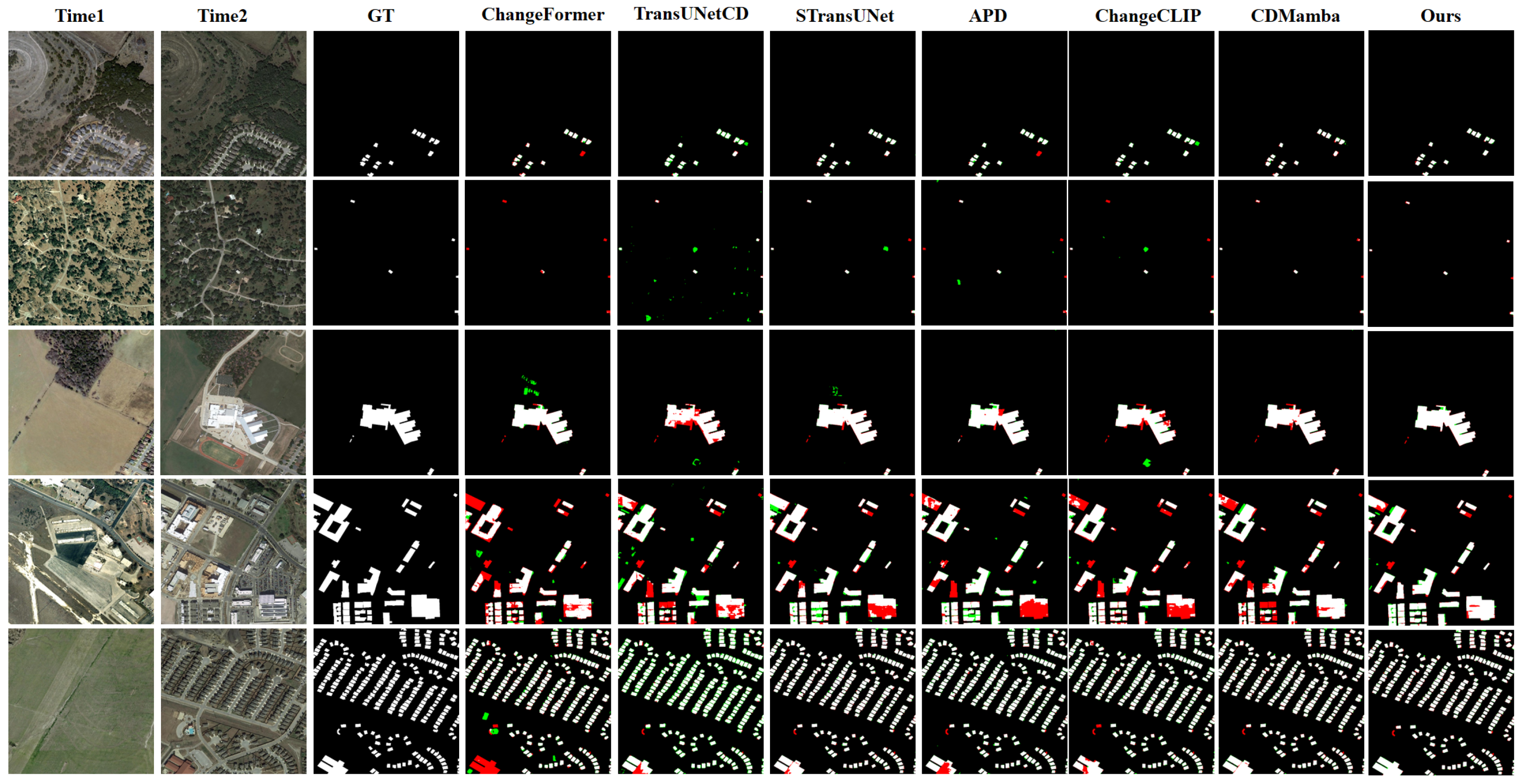
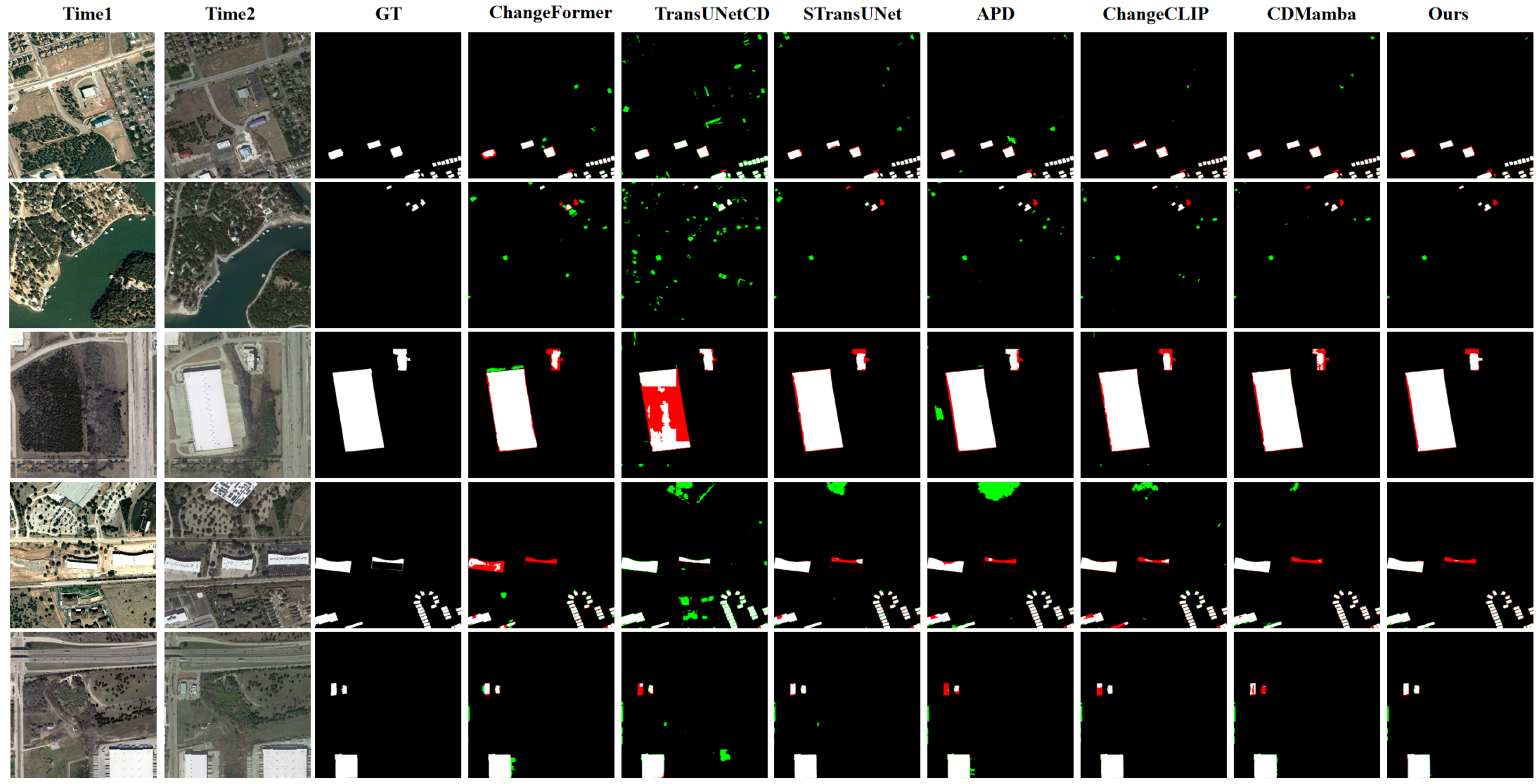
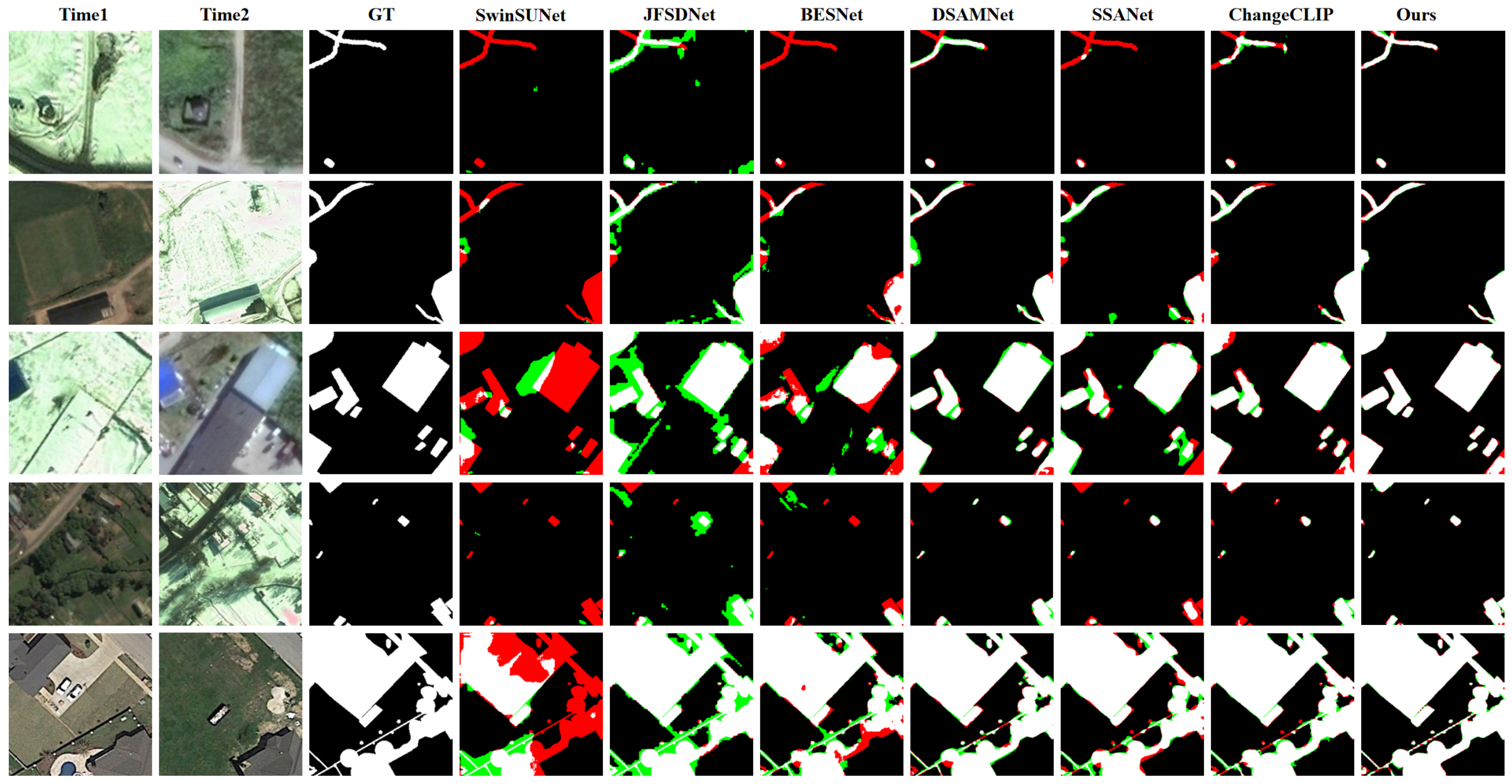
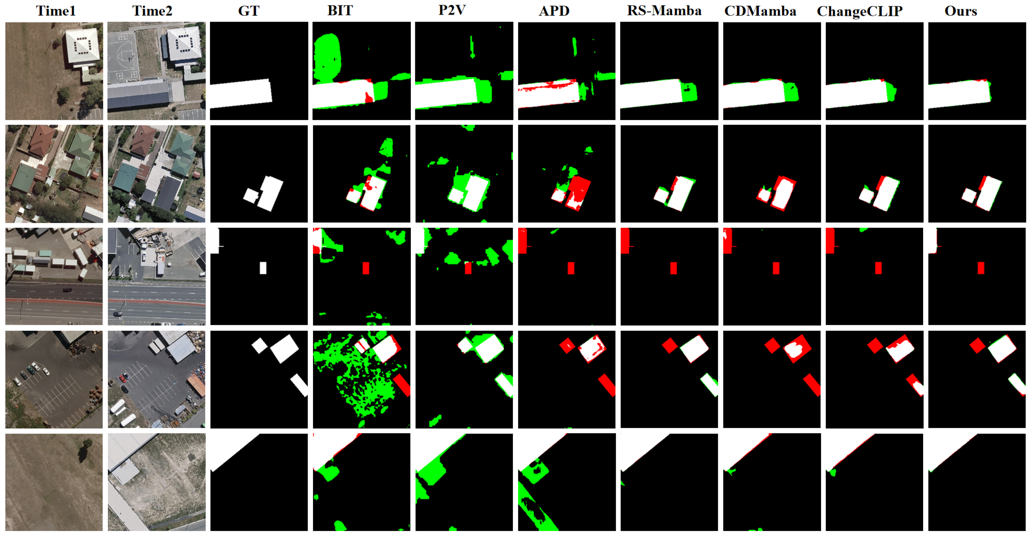
To provide an intuitive understanding of the performance, we visualize typical examples from the four datasets in Figure 4, Figure 5, Figure 6, Figure 7 and Figure 8. On LEVIR-CD and LEVIR-CD+ (Figure 4 and Figure 5), which involve complex building structures and shadows, competing methods such as ChangeCLIP and APD often suffer from boundary errors or missed detections in occluded areas. In contrast, CSD-Net⁺ produces more complete building masks that align well with the ground truth as the MLLM provides semantic localization while SAM delivers tight instance masks with sharp boundaries, and the three-way fusion preserves the pixel-level precision of the base model in confident regions.

On the CDD dataset (Figure 7), characterized by strong seasonal changes, our predictions remain stable across foliage, crop fields, and water surfaces, suppressing many false alarms caused by color or texture shifts. This supports the view that the content–style decoupling module learns features less sensitive to dominant style variations. On WHU (Figure 8), our method yields clean building footprints even in dense urban districts, with fewer spurious detections on roads and parking lots.

4.3.2. Visualization of Content–Style Decoupling

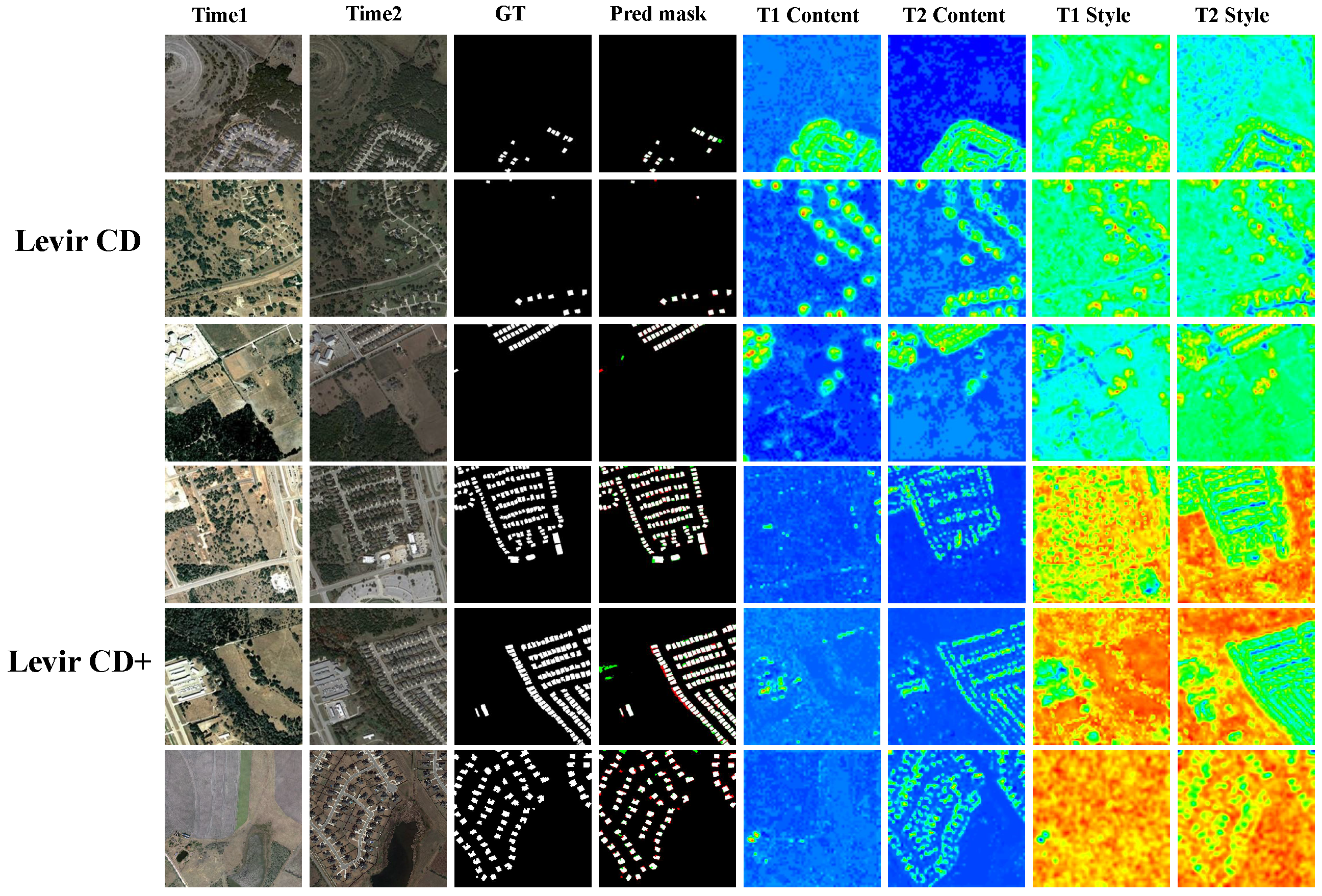
To better understand the behavior of the CSD module, we visualize the decoupled content and style features in Figure 9. The content maps concentrate on the intrinsic structure of human-made objects, such as building footprints and road layouts, while being largely invariant to lighting and seasonal changes. For the style branch, note that the final $S_{\mathrm{map}}^t$ is spatially invariant due to the broadcast constraint (Section 3.2); therefore, the “Style” column in Figure 9 visualizes the spatial response prior to global pooling/broadcasting. These maps reveal where the model attends to environmentally sensitive cues (e.g., vegetation, shadows) to estimate a global season/illumination vector, which is then broadcast and applied as feature-level compensation.

These observations are consistent across LEVIR-CD and LEVIR-CD+ (top and bottom of Figure 9), suggesting that the pseudo-change tokens and dual-stream transformer decoder help separate style-related variations from semantic structures. This provides a useful base prior for subsequent refinement.

Interpreting pseudo-change tokens. Beyond performance gains, the pseudo-change tokens P provide an interpretable style-prototype view. Rather than being designed to encode specific object textures (e.g., “grass leaves”), each token is encouraged to summarize common global imaging conditions in the dataset (e.g., “shadowed” vs. “illuminated”, “wet” vs. “dry”, or “hazy” vs. “clear”). Through cross-attention, image features query these prototypes to synthesize the current scene’s global environmental prior, which is then constrained by the spatially-invariant broadcast operation into $S_{\mathrm{map}}^t$. The style-response visualization in Figure 9 provides qualitative evidence that these responses tend to concentrate on environmentally sensitive cues such as vegetation and shadows, rather than object boundaries alone. We note, however, that this is an interpretability analysis rather than a complete proof of token semantics.

4.4. Effectiveness of Cognitive Semantic Reasoning

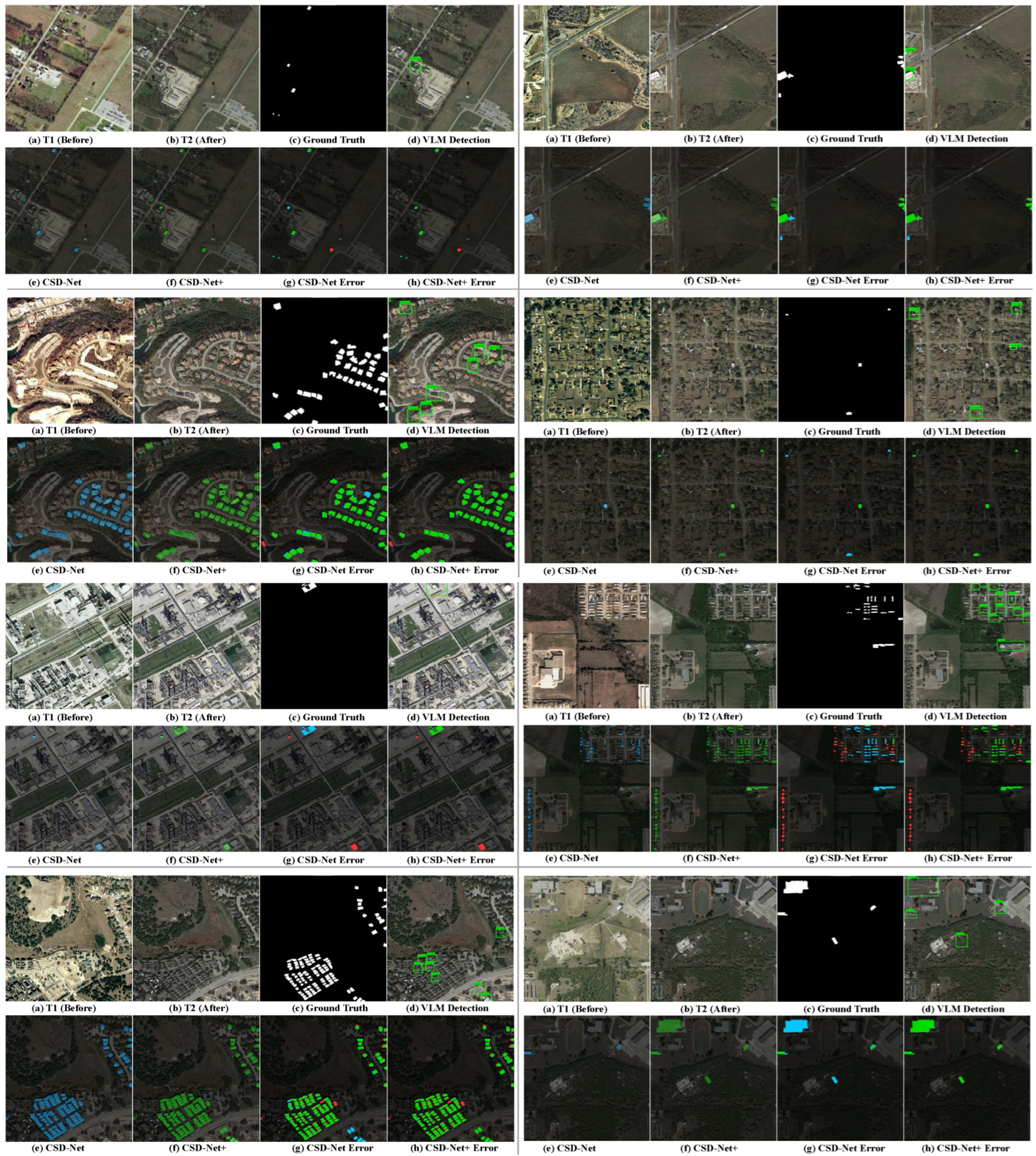
To assess how the MLLM+SAM refinement improves the base predictions, we present detailed case studies in Figure 6. We compare the outputs of CSD-Net (Base) (column (e)) and CSD-Net⁺ (column (f)) and visualize the MLLM’s refined detection boxes (column (d)) as well as the error maps.

Addressing missed detections (false negative recovery). In the first two rows, small or heavily occluded buildings are partially missed by the base model (red regions in the error maps). With spatial prompts derived from uncertain regions, the MLLM classifies these candidates as changes, and SAM generates tight instance masks with sharp boundaries to recover the missing buildings. This suggests that the MLLM provides useful semantic localization, while SAM delivers pixel-accurate masks.

Correcting false alarms (false positive suppression). In rows 3–4, elongated roads and parking lots are sometimes misclassified as changed buildings by the base model (green regions). The MLLM, guided by both the bi-temporal images and the candidate boxes, classifies these regions as no-change. The negative evidence ${\mathbf{M}}_{-}$ then suppresses these false positives via the three-way fusion, leading to cleaner final masks in CSD-Net⁺.

Object-level completion. In rows 5–6, large building complexes are fragmented by CSD-Net (Base) due to complex inner structures and shadows. The MLLM tends to treat them as holistic entities at the instance level and classifies them as changes. SAM then generates complete instance masks that, when fused with the base probability map via positive evidence ${\mathbf{M}}_{+}$, result in more complete and compact building footprints with accurate boundaries.

Overall, these examples suggest that the integration of MLLM+SAM can complement pure pixel-level matching in selected hard cases: the MLLM provides semantic localization, SAM delivers tight instance masks, and the three-way fusion enables simultaneous false negative recovery and false positive suppression.

4.5. Ablation Studies

4.5.1. Effect of Content–Style Decoupling

We conducted controlled ablation studies to evaluate the effectiveness of the proposed content–style decoupling (CSD) module and its associated losses. To ensure fair comparison, we systematically vary one component at a time while keeping others fixed. Starting from the full CSD-Net (Base), we derive four variants:

• w/o Decoupling: remove the dual-decoder structure and learnable pseudo-change tokens, directly feeding the deepest features $F_d^{t_1},F_d^{t_2}$ into the Bi-FPN. Loss: ${\mathcal{L}}_{\mathrm{base}}$ only (i.e., dropping both ${\mathcal{L}}_{\mathrm{recon}}$ and ${\mathcal{L}}_{\mathrm{const}}$).
• w/o ${\mathcal{L}}_{\mathrm{recon}}$: keep the full dual-decoder CSD structure but drop the reconstruction loss in Equation (20). Loss: ${\mathcal{L}}_{\mathrm{base}}+{\mathcal{L}}_{\mathrm{const}}$.
• w/o ${\mathcal{L}}_{\mathrm{const}}$: keep the full dual-decoder CSD structure but drop the content consistency loss in Equation (21). Loss: ${\mathcal{L}}_{\mathrm{base}}+{\mathcal{L}}_{\mathrm{recon}}$.
• w/o PM: remove the perturbation module (PM) in all encoder stages, while keeping the full CSD structure and all losses.

Table 6. Controlled ablation of the content–style decoupling (CSD) module. Numbers indicate IoU (%) on each dataset. Each variant modifies exactly one component to isolate its contribution.

Variant	LEVIR-CD	LEVIR-CD+	CDD	WHU
Full CSD-Net (Base)	85.35	75.82	96.05	90.35
w/o Decoupling	84.00	74.30	94.70	89.05
w/o ${\mathcal{L}}_{\mathrm{recon}}$	84.85	75.30	95.55	89.85
w/o ${\mathcal{L}}_{\mathrm{const}}$	84.75	75.15	95.45	89.75
w/o PM	84.65	75.00	95.30	89.60

reports the IoU on the four datasets for these variants.

From Table 6, we observe the following trends. Removing the entire decoupling structure (w/o Decoupling) causes the most significant degradation (e.g., −1.35% IoU on LEVIR-CD, −1.33% on CDD), especially on datasets with severe pseudo-changes, supporting the importance of content–style separation for robustness. Dropping either the reconstruction loss (w/o ${\mathcal{L}}_{\mathrm{recon}}$) or the content consistency loss (w/o ${\mathcal{L}}_{\mathrm{const}}$) leads to moderate but consistent performance drops across all datasets (0.48–0.58% for ${\mathcal{L}}_{\mathrm{recon}}$, 0.58–0.65% for ${\mathcal{L}}_{\mathrm{const}}$), indicating that both information completeness and temporal invariance are useful for the proposed decomposition. The perturbation module (PM) also provides consistent gains (0.70–0.80% IoU) by enhancing discriminative channels and improving robustness to alignment errors during multi-scale feature extraction. These controlled ablations support the contribution of each component in our design.

4.5.2. Effect of MLLM+SAM Refinement and Fusion Strategy

We then studied the impact of the MLLM+SAM refinement stage and different fusion strategies between CSD-Net and Rex-Omni-R. We compared:

• Base only: using CSD-Net (Base) without any MLLM+SAM refinement.
• Union fusion: taking the pixel-wise union of the base mask and MLLM+SAM mask, i.e., ${\mathbf{M}}_{\mathrm{final}}={\mathbf{M}}_{\mathrm{base}}\cup {\mathbf{M}}_{+}$.
• Intersection fusion: taking the pixel-wise intersection, i.e., ${\mathbf{M}}_{\mathrm{final}}={\mathbf{M}}_{\mathrm{base}}\cap {\mathbf{M}}_{+}$.
• Uncertainty-aware fusion (ours): using the adaptive weighted combination based on pixel-wise entropy (Section 3.5, Equation (48)).

Table 7. Ablation of the MLLM+SAM refinement and fusion strategy. Numbers indicate IoU/F1 (%) on LEVIR-CD and LEVIR-CD+. The three-way softmax fusion achieves the best balance between precision and recall.

Method	LEVIR-CD	LEVIR-CD+
Base only (CSD-Net)	85.35/92.08	75.82/86.25
+ Union fusion	85.70/92.20	76.28/86.60
+ Intersection fusion	84.92/92.30	75.45/86.48
+ Uncertainty-aware fusion (ours)	85.88/92.38	76.45/87.10

summarizes the IoU and F1 results on LEVIR-CD and LEVIR-CD+.

The results in Table 7 reveal several important insights. Union fusion improves recall by accepting all MLLM+SAM detections, leading to moderate IoU gains (+0.35% on LEVIR-CD, +0.46% on LEVIR-CD+) but may introduce extra false positives, resulting in limited F1 improvement. Intersection fusion causes IoU degradation (−0.43% on LEVIR-CD, −0.37% on LEVIR-CD+), despite slightly higher precision. This occurs because (i) the MLLM+SAM mask ${\mathbf{M}}_{+}$ is inherently sparse—SAM is prompted only on positively refined boxes, covering a small subset of changed pixels, so intersection discards many true positive pixels correctly detected by the base model, and (ii) SAM’s mask boundaries occasionally under-segment complex structures (e.g., buildings with heterogeneous rooftops), further shrinking the intersection region. These findings highlight that simple set operations cannot effectively combine the complementary strengths of the two stages: the base model provides dense, high-recall coverage while the MLLM+SAM pipeline contributes sparse, high-precision corrections. Our three-way softmax fusion resolves this by adaptively blending evidence based on pixel-wise uncertainty, achieving the best balance (+0.53% IoU and +0.30% F1 on LEVIR-CD, +0.63% IoU and +0.85% F1 on LEVIR-CD+). The negative evidence ${\mathbf{M}}_{-}$ additionally suppresses false positives via denominator inflation, a mechanism absent in both union and intersection baselines.

4.6. Complexity and Efficiency Analysis

In addition to accuracy, computational efficiency is crucial for practical deployment of change detection models. To follow a tiered evaluation strategy and ensure fair comparison with existing specialized small models, we primarily analyze the complexity of CSD-Net (Base) alone—without Stage 2 (MLLM+SAM) refinement—because most competing methods are pure-vision detectors. In this setting, the base model already achieves strong performance under comparable computational budgets, making it the recommended choice for real-time or large-scale deployment. We then discuss CSD-Net⁺ as an optional cognitive enhancement for offline, quality-critical scenarios.

Measurement protocol. Complexity metrics of CSD-Net (Base) are measured using thop (PyTorch-OpCounter) with a standardized input resolution of $256\times 256\times 3$ for bi-temporal image pairs. We count: (i) all parameters in the Siamese encoder, dual-decoder CSD module, Bi-FPN, and prediction heads and (ii) FLOPs for one forward pass including all convolutional, normalization, and attention operations. Frozen or auxiliary components (e.g., learnable pseudo-change tokens, which add only 4K parameters) are included for completeness. For other methods, we report complexity numbers as available in the corresponding original papers for reference.

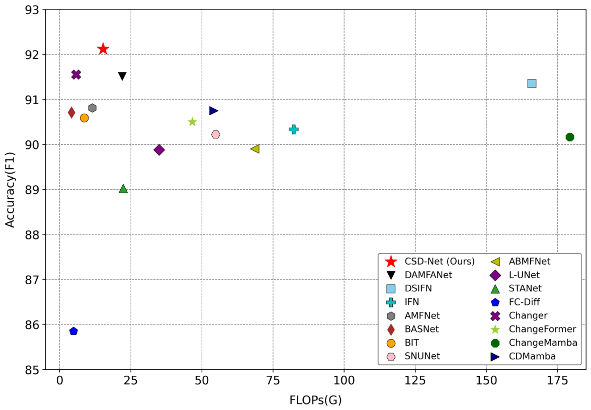
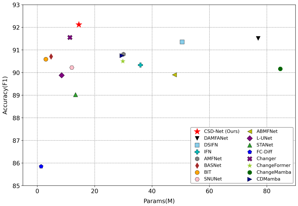
Figure 10 and Figure 11 summarize the small-model efficiency comparison (F1-scores are the same as those reported in the quantitative comparison (Table 2) or in the corresponding original papers) on LEVIR-CD for representative change detection networks, including IFN, STANet, Changer, ChangeFormer, FC-Diff, and SNU-Net. We report their complexity in

Table 8. Complexity and efficiency comparison of change detection models. FPS measured on a single NVIDIA RTX 3090 (NVIDIA Corporation, Santa Clara, CA, USA) with $256\times 256$ input, averaged over 100 forward passes.

Method	Params (M)	FLOPs (G)	FPS
DAMFANet [63]	77.00	22.00	22
DSIFN [49]	50.50	166.00	8
IFNet [49]	35.99	82.26	13
AMFNet [64]	30.05	11.50	42
BASNet [65]	4.80	4.20	85
BIT [5]	2.99	8.67	55
SNU-Net [52]	12.03	54.83	18
ABMFNet	47.80	68.50	14
L-UNet [50]	8.50	35.00	25
STANet [4]	13.36	22.38	30
FC-Diff [1]	1.35	4.86	75
Changer [66]	11.39	5.78	62
ChangeFormer [21]	3.85	1.39	90
ChangeMamba [47]	84.70	179.32	6
CDMamba [23]	29.53	54.18	17
CSD-Net (Base)	14.49	15.26	32
CSD-Net+ (w/ MLLM+SAM)	3214.49 †	2815.26 †	0.3 †

^† Stage 2 overhead includes Qwen2.5-3B (LoRA, ≈2% trainable) + SAM-ViT-H. CSD-Net⁺ is designed for offline, quality-critical refinement and is not recommended for real-time deployment.

for easier reading.

Parameter breakdown. CSD-Net (Base) contains 14.49M parameters in total. Most parameters are contributed by the Siamese encoder, the CSD module, and the decoder head, while the learnable pseudo-change tokens add only a negligible overhead.

Stage 2 overhead. The MLLM and SAM are optional refinement modules used only in the second stage. Their computational overhead is not included in the base complexity comparison, which focuses on the pure-vision CSD-Net (Base). To make the cost of this optional stage explicit,

Table 9. Component-level complexity of the optional Stage 2 refinement. Values are approximate because the number of MLLM queries and SAM prompts varies with the base prediction uncertainty. FPS is measured on a single NVIDIA RTX 3090 (NVIDIA Corporation, Santa Clara, CA, USA) with $256\times 256$ input.

Component	Params (M)	FLOPs (G)	FPS	Role
CSD-Net (Base)	14.49	15.26	32.0	Dense base prior and coarse proposal generation
Rex-Omni-R/Qwen2.5-3B	≈2560	≈2520	≈0.4	Proposal-level semantic box refinement and change/no-change decision
SAM-ViT-H	≈640	≈280	≈1.5	Box-prompted instance mask refinement for positive proposals
Three-way fusion	<$0.01$	<$0.01$	>100	Pixel-wise fusion of base, positive, and negative evidence
CSD-Net+ total	≈3214.49	≈2815.26	≈0.3	Offline, quality-critical refinement

reports an approximate component-level breakdown measured or estimated using the same $256\times 256$ inference setting. The exact cost of the MLLM branch depends on the number of generated coarse proposals and output tokens, while the SAM cost depends on the number of positively refined boxes.

Several observations can be made from Figure 10 and Figure 11. CSD-Net (Base) remains lightweight (14.49M parameters and 15.26G FLOPs) while achieving strong accuracy, indicating a favorable accuracy–efficiency trade-off in the small-model regime. This supports our tiered recommendation: the base model is suitable for real-time or large-scale deployment, while Stage 2 serves as an optional offline cognitive enhancement for quality-critical scenarios.

Finally, this complexity analysis pertains to the base model only. Stage 2 (MLLM+SAM) is an optional offline refinement module; its overhead is not included in the base complexity comparison. The core CSD-Net (Base) already delivers competitive accuracy with a reasonable computational budget, making it suitable for large-scale deployment, while CSD-Net⁺ provides additional accuracy for quality-critical offline applications. This tiered design offers flexibility across diverse operational constraints.

Tiered usage recommendation. We explicitly acknowledge that Stage 2 (CSD-Net⁺) introduces significant overhead in latency and memory due to the MLLM and SAM. We therefore position it as an optional semantic refiner for offline, quality-critical applications, where the goal is to improve difficult, semantically ambiguous cases when additional computation is acceptable. In contrast, for real-time deployment or large-scale processing, we recommend the base CSD-Net as the default option as it already provides a strong accuracy–efficiency trade-off in the small-model regime (Figure 10 and Figure 11).

5. Discussion

The experimental results suggest that style-aware content–style decoupling is an effective way to reduce pseudo-change interference in remote sensing change detection. Compared with conventional feature-difference detectors, CSD-Net explicitly encourages the network to separate content-dominant features from global environmental/style factors, which is particularly useful with seasonal, illumination, and atmospheric variations. The consistent improvements on LEVIR-CD, LEVIR-CD+, CDD, and WHU indicate that the proposed pseudo-change tokens and dual-decoder design improve robustness without requiring a heavy foundation model at the default deployment stage.

The optional CSD-Net⁺ pipeline further shows that foundation models can be useful when they are used as constrained refiners rather than free-form dense predictors. By converting uncertain regions into spatial prompts, Rex-Omni-R is guided to make proposal-level change/no-change decisions and to refine candidate boxes, while SAM converts positively refined boxes into sharper instance masks. The three-way uncertainty-aware fusion then integrates positive and negative evidence only where the base model is uncertain. This design helps suppress semantically implausible false alarms and recover missed objects in difficult cases. However, the gains of Stage 2 are modest relative to its cost: CSD-Net⁺ introduces approximately 3.2B additional parameters and roughly two orders of magnitude higher inference cost, while improving IoU by 0.45–2.20% over the already strong base model. Therefore, we recommend CSD-Net (Base) for real-time or large-scale processing and reserve CSD-Net⁺ for offline, quality-critical applications.

Several limitations should be considered when interpreting these results. First, the current framework focuses on binary change detection and does not explicitly model fine-grained semantic transitions, such as “what changed into what”. Second, the style branch approximates dominant environmental variations as a global style/radiometric bias after broadcast. This assumption is useful for image-level illumination or seasonal tone shifts, but it may be insufficient for strongly localized shadows, partial haze, non-uniform sensor artifacts, or spatially heterogeneous vegetation changes. Third, the framework assumes that the bi-temporal images are reasonably co-registered before change detection. Residual geometric misregistration can introduce boundary-level false positives and false negatives that are not explicitly modeled by the CSD module, especially for small objects and dense urban structures.

The optional MLLM+SAM refiner also has practical limitations. It relies on curated refinement-style prompts and proposal annotations, and its behavior may be sensitive to cross-city, cross-sensor, or rare-category domain shifts. Moreover, we did not conduct an isolated quantitative analysis of MLLM refinement accuracy, confidence calibration, hallucination frequency, or SAM mask quality across object sizes and boundary types. These issues indicate that future work should investigate more robust, calibration-aware, and computationally efficient refinement strategies. A promising direction is to distill the semantic reasoning capability of the MLLM+SAM pipeline into a compact change-aware head, thus retaining most of the refinement benefit with negligible additional inference cost.

6. Conclusions

In this paper, we presented CSD-Net, a style-aware content–style decoupling network for robust remote sensing change detection and its coarse-to-fine extension CSD-Net⁺. The key idea is to encourage separation between intrinsic semantic content and extrinsic environmental style using learnable pseudo-change tokens and a dual-stream transformer decoder while enforcing reconstruction and temporal consistency constraints. Built upon this decoupled representation and a Bi-FPN decoder, the base model achieves strong performance, competitive with or surpassing previous methods on four challenging benchmarks (LEVIR-CD, LEVIR-CD+, CDD, and WHU), particularly improving robustness to seasonal and illumination-induced pseudo-changes.

To further handle semantically ambiguous cases, we introduced a spatially guided visual instruction tuning scheme that adapts a Qwen2.5-3B multimodal model initialized from the Rex-Omni checkpoint [13] into a semantic refiner (Rex-Omni-R), coupled with SAM-based instance mask refinement and a novel three-way uncertainty-aware softmax fusion mechanism. The base model generates coarse proposal boxes from uncertain regions; Rex-Omni-R refines each proposal by outputting a tighter box and a change/no-change decision with a confidence score; SAM then converts positively refined boxes into pixel-accurate instance masks with sharp boundaries. The three-way fusion integrates: (i) the base prior ${\mathbf{P}}_{\mathrm{base}}$, (ii) SAM-refined positive evidence ${\mathbf{M}}_{+}$ for false negative recovery, and (iii) negative evidence ${\mathbf{M}}_{-}$ for false positive suppression. Pixel-wise uncertainty dynamically amplifies the influence of Stage 2 evidence only in regions where the base model is ambiguous, while reliability scores filter potential hallucinations. This two-stage framework consistently improves IoU by 0.45–2.20% and F1 by 0.30–1.37% across all datasets compared to the already strong base model. The qualitative analyses on hard cases indicate that the refiner provides semantic-guided box tightening while SAM delivers tight instance masks, recovering missed objects and suppressing semantically implausible false alarms in selected uncertain regions.

In future work, we plan to extend CSD-Net towards semantic change understanding, where each changed region is not only localized but also assigned a category of what has changed into what. We are also interested in exploring self-supervised or weakly supervised variants of the content–style decoupling module on large-scale multi-temporal archives and evaluating the proposed framework with stronger domain shifts, including cross-city, cross-sensor, and multi-temporal scenarios. We believe that combining style-aware representations with scalable multimodal reasoning will open up new possibilities for trustworthy and interpretable remote sensing change analysis.

References

1. Daudt, R.C.; Le Saux, B.; Boulch, A. Fully convolutional siamese networks for change detection. In 2018 25th IEEE International Conference on Image Processing (ICIP); IEEE: Piscataway, NJ, USA, 2018; pp. 4063–4067. [Google Scholar]
2. Zhou, Z.; Siddiquee, M.M.R.; Tajbakhsh, N.; Liang, J. UNet++: A Nested U-Net Architecture for Medical Image Segmentation. In Deep Learning in Medical Image Analysis and Multimodal Learning for Clinical Decision Support; Springer: Cham, Switzerland, 2018; Volume 11045, pp. 3–11. [Google Scholar] [CrossRef] [PubMed]
3. Chen, J.; Yuan, Z.; Peng, J.; Chen, L.; Huang, H.; Zhu, J.; Liu, Y.; Li, H. DASNet: Dual attentive fully convolutional Siamese networks for change detection in high-resolution satellite images. IEEE J. Sel. Top. Appl. Earth Obs. Remote Sens. 2020, 14, 1194–1206. [Google Scholar]
4. Chen, H.; Shi, Z. A Spatial-Temporal Attention-Based Method and a New Dataset for Remote Sensing Image Change Detection. Remote Sens. 2020, 12, 1662. [Google Scholar] [CrossRef]
5. Chen, H.; Qi, Z.; Shi, Z. Remote Sensing Image Change Detection with Transformers. IEEE Trans. Geosci. Remote Sens. 2021, 60, 5607514. [Google Scholar] [CrossRef]
6. Zhang, C.; Wang, L.; Cheng, S.; Li, Y. SwinSUNet: Pure Transformer Network for Remote Sensing Image Change Detection. IEEE Trans. Geosci. Remote Sens. 2022, 60, 5224713. [Google Scholar] [CrossRef]
7. Radford, A.; Kim, J.W.; Hallacy, C.; Ramesh, A.; Goh, G.; Agarwal, S.; Sastry, G.; Askell, A.; Mishkin, P.; Clark, J.; et al. Learning transferable visual models from natural language supervision. In Proceedings of the International Conference on Machine Learning, Virtual, 18–24 July 2021; pp. 8748–8763. [Google Scholar]
8. Dong, S.; Wang, L.; Du, B.; Meng, X. ChangeCLIP: Remote sensing change detection with multimodal vision-language representation learning. ISPRS J. Photogramm. Remote Sens. 2024, 208, 53–69. [Google Scholar] [CrossRef]
9. Sun, X.; Wang, P.; Lu, W.; Zhu, Z.; Lu, X.; He, Q.; Li, J.; Rong, X.; Yang, Z.; Chang, H.; et al. RingMo: A remote sensing foundation model with masked image modeling. IEEE Trans. Geosci. Remote Sens. 2022, 61, 5612822. [Google Scholar] [CrossRef]
10. Kuckreja, K.; Danish, M.S.; Naseer, M.; Das, A.; Khan, S.; Khan, F.S. Geochat: Grounded large vision-language model for remote sensing. IEEE Proc. CVF Conf. Comput. Vis. Pattern Recognit. 2024, 2, 4. [Google Scholar]
11. Guo, X.; Lao, J.; Dang, B.; Zhang, Y.; Yu, L.; Ru, L.; Zhong, L.; Huang, Z.; Wu, K.; Hu, D.; et al. Skysense: A multi-modal remote sensing foundation model towards universal interpretation for earth observation imagery. In Proceedings of the IEEE/CVF Conference on Computer Vision and Pattern Recognition, Vancouver, BC, Canada, 16–22 June 2024; pp. 27672–27683. [Google Scholar]
12. Hu, Y.; Yuan, J.; Wen, C.; Lu, X.; Liu, Y.; Li, X. Rsgpt: A remote sensing vision language model and benchmark. ISPRS J. Photogramm. Remote Sens. 2025, 224, 272–286. [Google Scholar] [CrossRef]
13. Jiang, Q.; Huo, J.; Chen, X.; Xiong, Y.; Zeng, Z.; Chen, Y.; Ren, T.; Yu, J.; Zhang, L. Detect Anything via Next Point Prediction. arXiv 2025, arXiv:2510.12798. [Google Scholar]
14. Kirillov, A.; Mintun, E.; Ravi, N.; Mao, H.; Rolland, C.; Gustafson, L.; Xiao, T.; Whitehead, S.; Berg, A.C.; Lo, W.Y.; et al. Segment Anything. In Proceedings of the IEEE/CVF International Conference on Computer Vision (ICCV), Paris, France, 2–3 October 2023; pp. 4015–4026. [Google Scholar]
15. Lebedev, M.; Vizilter, Y.V.; Vygolov, O.; Knyaz, V.A.; Rubis, A.Y. Change detection in remote sensing images using conditional adversarial networks. Int. Arch. Photogramm. Remote Sens. Spat. Inf. Sci. 2018, 42, 565–571. [Google Scholar] [CrossRef]
16. Ji, S.; Wei, S.; Lu, M. Fully Convolutional Networks for Multisource Building Extraction From an Open Aerial and Satellite Imagery Data Set. IEEE Trans. Geosci. Remote Sens. 2019, 57, 574–586. [Google Scholar] [CrossRef]
17. Parelius, E.J. A Review of Deep-Learning Methods for Change Detection in Multispectral Remote Sensing Images. Remote Sens. 2023, 15, 2092. [Google Scholar] [CrossRef]
18. Alcantarilla, P.F.; Stent, S.; Ros, G.; Arroyo, R.; Gherardi, R. Street-view change detection with deconvolutional networks. Auton. Robot. 2018, 42, 1301–1322. [Google Scholar] [CrossRef]
19. Song, X.; Hua, Z.; Li, J. Remote Sensing Image Change Detection Transformer Network Based on Dual-Feature Mixed Attention. IEEE Trans. Geosci. Remote Sens. 2022, 60, 5920416. [Google Scholar] [CrossRef]
20. Feng, Y.; Xu, H.; Jiang, J.; Liu, H.; Zheng, J. ICIF-Net: Intra-Scale Cross-Interaction and Inter-Scale Feature Fusion Network for Bitemporal Remote Sensing Images Change Detection. IEEE Trans. Geosci. Remote Sens. 2022, 60, 4410213. [Google Scholar] [CrossRef]
21. Bandara, W.G.C.; Patel, V.M. A transformer-based siamese network for change detection. In IGARSS 2022—2022 IEEE International Geoscience and Remote Sensing Symposium; IEEE: Piscataway, NJ, USA, 2022; pp. 207–210. [Google Scholar]
22. Zhao, S.; Chen, H.; Zhang, X.; Xiao, P.; Bai, L.; Ouyang, W. RS-Mamba for Large Remote Sensing Image Dense Prediction. IEEE Trans. Geosci. Remote Sens. 2024, 62, 5633314. [Google Scholar] [CrossRef]
23. Zhang, H.; Chen, K.; Liu, C.; Chen, H.; Zou, Z.; Shi, Z. CDMamba: Incorporating Local Clues Into Mamba for Remote Sensing Image Binary Change Detection. IEEE Trans. Geosci. Remote Sens. 2025, 63, 4405016. [Google Scholar] [CrossRef]
24. Liu, J.; Zhang, W.; Liu, F.; Xiao, L. A Probabilistic Model Based on Bipartite Convolutional Neural Network for Unsupervised Change Detection. IEEE Trans. Geosci. Remote Sens. 2022, 60, 4701514. [Google Scholar] [CrossRef]
25. Wei, J.; Sun, K.; Li, W.; Li, W.; Gao, S.; Miao, S.; Tan, Y.; Cui, W.; Duan, Y. Cross-Visual Style Change Detection for Remote Sensing Images via Representation Consistency Deep Supervised Learning. Remote Sens. 2025, 17, 798. [Google Scholar] [CrossRef]
26. Wang, S.; Li, Y.; Xie, M.; Chi, M.; Wang, Y.; Wang, C.; Zhu, W. Align, perturb and decouple: Toward better leverage of difference information for RSI change detection. In Proceedings of the Thirty-Second International Joint Conference on Artificial Intelligence (IJCAI ’23), Macao, China, 19–25 August 2023; pp. 1497–1505. [Google Scholar] [CrossRef] [PubMed]
27. Rahhal, M.M.A.; Bazi, Y.; Alsharif, N.A.; Bashmal, L.; Alajlan, N.; Melgani, F. Multilanguage Transformer for Improved Text to Remote Sensing Image Retrieval. IEEE J. Sel. Top. Appl. Earth Obs. Remote Sens. 2022, 15, 9115–9126. [Google Scholar] [CrossRef]
28. Tang, X.; Wang, Y.; Ma, J.; Zhang, X.; Liu, F.; Jiao, L. Interacting-Enhancing Feature Transformer for Cross-Modal Remote-Sensing Image and Text Retrieval. IEEE Trans. Geosci. Remote Sens. 2023, 61, 5611715. [Google Scholar] [CrossRef]
29. Wang, W.; Chen, Z.; Chen, X.; Wu, J.; Zhu, X.; Zeng, G.; Luo, P.; Lu, T.; Zhou, J.; Qiao, Y.; et al. Visionllm: Large language model is also an open-ended decoder for vision-centric tasks. NeurIPS 2023, 36, 61501–61513. [Google Scholar] [CrossRef]
30. Liu, H.; Li, C.; Wu, Q.; Lee, Y.J. Visual Instruction Tuning. NeurIPS 2023, 36, 34892–34916. [Google Scholar] [CrossRef]
31. Dai, W.; Li, J.; Li, D.; Tiong, A.M.H.; Zhao, J.; Wang, W.; Li, B.; Fung, P.; Hoi, S.C.H. InstructBLIP: Towards General-purpose Vision-Language Models with Instruction Tuning. NeurIPS 2023, 36, 49250–49267. [Google Scholar] [CrossRef]
32. Chen, K.; Zhang, Z.; Zeng, W.; Zhang, R.; Zhu, F.; Zhao, R. Shikra: Unleashing Multimodal LLM’s Referential Dialogue Magic. arXiv 2023, arXiv:2306.15195. [Google Scholar]
33. Peng, Z.; Wang, W.; Dong, L.; Hao, Y.; Huang, S.; Ma, S.; Wei, F. Kosmos-2: Grounding multimodal large language models to the world. arXiv 2023, arXiv:2306.14824. [Google Scholar]
34. Liu, S.; Zeng, Z.; Ren, T.; Li, F.; Zhang, H.; Yang, J.; Jiang, Q.; Li, C.; Yang, J.; Su, H.; et al. Grounding dino: Marrying dino with grounded pre-training for open-set object detection. arXiv 2023, arXiv:2303.05499. [Google Scholar]
35. Jiang, Q.; Li, F.; Ren, T.; Liu, S.; Zeng, Z.; Yu, K.; Zhang, L. T-rex: Counting by visual prompting. arXiv 2023, arXiv:2311.13596. [Google Scholar]
36. Jiang, Q.; Li, F.; Zeng, Z.; Ren, T.; Liu, S.; Zhang, L. T-rex2: Towards generic object detection via text-visual prompt synergy. In Proceedings of the European Conference on Computer Vision, Milan, Italy, 29 September–4 October 2024; pp. 38–57. [Google Scholar]
37. Jiang, Q.; Chen, X.; Zeng, Z.; Yu, J.; Zhang, L. Rex-Thinker: Grounded Object Referring via Chain-of-Thought Reasoning. arXiv 2025, arXiv:2506.04034. [Google Scholar]
38. Tong, S.; Liu, Z.; Zhai, Y.; Ma, Y.; LeCun, Y.; Xie, S. Eyes wide shut? exploring the visual shortcomings of multimodal llms. arXiv 2024, arXiv:2401.06209. [Google Scholar]
39. Zhang, W.; Cai, M.; Zhang, T.; Zhuang, Y.; Mao, X. EarthGPT: A universal multimodal large language model for multisensor image comprehension in remote sensing domain. IEEE Trans. Geosci. Remote Sens. 2024, 62, 5917820. [Google Scholar] [CrossRef]
40. Deng, P.; Zhou, W.; Wu, H. Changechat: An interactive model for remote sensing change analysis via multimodal instruction tuning. In ICASSP 2025—2025 IEEE International Conference on Acoustics, Speech and Signal Processing (ICASSP); IEEE: Piscataway, NJ, USA, 2025; pp. 1–5. [Google Scholar]
41. Mao, Z.; Tong, X.; Luo, Z.; Zhang, H. MFATNet: Multi-Scale Feature Aggregation via Transformer for Remote Sensing Image Change Detection. Remote Sens. 2022, 14, 5379. [Google Scholar] [CrossRef]
42. Wang, L.; Li, H. HMCNet: Hybrid Efficient Remote Sensing Images Change Detection Network Based on Cross-Axis Attention MLP and CNN. IEEE Trans. Geosci. Remote Sens. 2022, 60, 5236514. [Google Scholar] [CrossRef]
43. Li, Q.; Zhong, R.; Du, X.; Du, Y. TransUNetCD: A Hybrid Transformer Network for Change Detection in Optical Remote-Sensing Images. Trans. Geosci. Remote Sens. 2022, 60, 5622519. [Google Scholar] [CrossRef]
44. Pei, G.; Zhang, L. Feature Hierarchical Differentiation for Remote Sensing Image Change Detection. IEEE Geosci. Remote Sens. Lett. 2022, 19, 6514105. [Google Scholar] [CrossRef]
45. Yuan, J.; Wang, L.; Cheng, S. STransUNet: A Siamese TransUNet-Based Remote Sensing Image Change Detection Network. IEEE J. Sel. Top. Appl. Earth Obs. Remote Sens. 2022, 15, 9241–9253. [Google Scholar] [CrossRef]
46. Ye, Y.; Wang, M.; Zhou, L.; Lei, G.; Fan, J.; Qin, Y. Adjacent-Level Feature Cross-Fusion with 3-D CNN for Remote Sensing Image Change Detection. IEEE Trans. Geosci. Remote Sens. 2023, 61, 5618214. [Google Scholar] [CrossRef]
47. Chen, H.; Song, J.; Han, C.; Xia, J.; Yokoya, N. ChangeMamba: Remote sensing change detection with spatiotemporal state space model. IEEE Trans. Geosci. Remote Sens. 2024, 62, 4409720. [Google Scholar] [CrossRef]
48. Daudt, R.C.; Le Saux, B.; Boulch, A.; Gousseau, Y. Multitask learning for large-scale semantic change detection. Comput. Vis. Image Underst. 2019, 187, 102783. [Google Scholar] [CrossRef]
49. Zhang, C.; Yue, P.; Tapete, D.; Jiang, L.; Shangguan, B.; Huang, L.; Liu, G. A deeply supervised image fusion network for change detection in high resolution bi-temporal remote sensing images. ISPRS J. Photogramm. Remote Sens. 2020, 166, 183–200. [Google Scholar] [CrossRef]
50. Papadomanolaki, M.; Vakalopoulou, M.; Karantzalos, K. A Deep Multitask Learning Framework Coupling Semantic Segmentation and Fully Convolutional LSTM Networks for Urban Change Detection. IEEE Trans. Geosci. Remote Sens. 2021, 59, 7651–7668. [Google Scholar] [CrossRef]
51. Liu, Y.; Pang, C.; Zhan, Z.; Zhang, X.; Yang, X. Building Change Detection for Remote Sensing Images Using a Dual-Task Constrained Deep Siamese Convolutional Network Model. IEEE Geosci. Remote Sens. Lett. 2021, 18, 811–815. [Google Scholar] [CrossRef]
52. Fang, S.; Li, K.; Shao, J.; Li, Z. SNUNet-CD: A Densely Connected Siamese Network for Change Detection of VHR Images. IEEE Geosci. Remote Sens. Lett. 2022, 19, 8007805. [Google Scholar] [CrossRef]
53. Shi, Q.; Liu, M.; Li, S.; Liu, X.; Wang, F.; Zhang, L. A Deeply Supervised Attention Metric-Based Network and an Open Aerial Image Dataset for Remote Sensing Change Detection. IEEE Trans. Geosci. Remote Sens. 2022, 60, 5604816. [Google Scholar] [CrossRef]
54. Lei, J.; Gu, Y.; Xie, W.; Li, Y.; Du, Q. Boundary Extraction Constrained Siamese Network for Remote Sensing Image Change Detection. IEEE Trans. Geosci. Remote Sens. 2022, 60, 5621613. [Google Scholar] [CrossRef]
55. Cheng, G.; Wang, G.; Han, J. ISNet: Towards Improving Separability for Remote Sensing Image Change Detection. IEEE Trans. Geosci. Remote Sens. 2022, 60, 5623811. [Google Scholar] [CrossRef]
56. Wan, L.; Tian, Y.; Kang, W.; Ma, L. D-TNet: Category-Awareness Based Difference-Threshold Alternative Learning Network for Remote Sensing Image Change Detection. IEEE Trans. Geosci. Remote Sens. 2022, 60, 5633316. [Google Scholar] [CrossRef]
57. Zhou, Y.; Feng, Y.; Huo, S.; Li, X. Joint Frequency-Spatial Domain Network for Remote Sensing Optical Image Change Detection. IEEE Trans. Geosci. Remote Sens. 2022, 60, 5627114. [Google Scholar] [CrossRef]
58. Ling, J.; Hu, L.; Cheng, L.; Chen, M.; Yang, X. IRA-MRSNet: A Network Model for Change Detection in High-Resolution Remote Sensing Images. Remote Sens. 2022, 14, 5598. [Google Scholar] [CrossRef]
59. Lu, K.; Huang, X. RCDT: Relational remote sensing change detection with transformer. arXiv 2022, arXiv:2212.04869. [Google Scholar]
60. Jiang, K.; Zhang, W.; Liu, J.; Liu, F.; Xiao, L. Joint Variation Learning of Fusion and Difference Features for Change Detection in Remote Sensing Images. IEEE Trans. Geosci. Remote Sens. 2022, 60, 4709918. [Google Scholar] [CrossRef]
61. Shu, Q.; Pan, J.; Zhang, Z.; Wang, M. DPCC-Net: Dual-perspective change contextual network for change detection in high-resolution remote sensing images. Int. J. Appl. Earth Obs. Geoinf. 2022, 112, 102940. [Google Scholar] [CrossRef]
62. Li, Z.; Yan, C.; Sun, Y.; Xin, Q. A Densely Attentive Refinement Network for Change Detection Based on Very-High-Resolution Bitemporal Remote Sensing Images. IEEE Trans. Geosci. Remote Sens. 2022, 60, 4409818. [Google Scholar] [CrossRef]
63. Ren, H.; Xia, M.; Weng, L.; Hu, K.; Lin, H. Dual-attention-guided multiscale feature aggregation network for remote sensing image change detection. IEEE J. Sel. Top. Appl. Earth Obs. Remote Sens. 2024, 17, 4899–4916. [Google Scholar] [CrossRef]
64. Zhan, Z.; Ren, H.; Xia, M.; Lin, H.; Wang, X.; Li, X. Amfnet: Attention-guided multi-scale fusion network for bi-temporal change detection in remote sensing images. Remote Sens. 2024, 16, 1765. [Google Scholar] [CrossRef]
65. Wang, Z.; Gu, G.; Xia, M.; Weng, L.; Hu, K. Bitemporal attention sharing network for remote sensing image change detection. IEEE J. Sel. Top. Appl. Earth Obs. Remote Sens. 2024, 17, 10368–10379. [Google Scholar] [CrossRef]
66. Fang, S.; Li, K.; Li, Z. Changer: Feature interaction is what you need for change detection. IEEE Trans. Geosci. Remote Sens. 2023, 61, 5610111. [Google Scholar] [CrossRef]
Figure 1. Motivation and overview of our coarse-to-fine RSCD framework. (a) A key failure mode of standard detectors is structure–environment entanglement: radiometric bias and intrinsic geometry are mixed in learned features, making feature disparity unreliable under domain shift conditions. (b) Proposed solution (CSD-Net+): A style-aware base predictor encourages intrinsic/extrinsic feature separation via pseudo-change tokens with spatially invariant broadcast subtraction to produce a robust base prior; optionally, uncertain regions are converted to box prompts, and a Cognitive-Aware Semantic Refiner (Qwen2.5-3B initialized from Rex-Omni, adapted via LoRA) refines coarse proposals into tighter boxes with change/no-change decisions, followed by SAM-based mask refinement and three-way uncertainty-aware fusion.
Remotesensing 18 02074 g001
Figure 2. The overall architecture of CSD-Net+. The framework consists of three phases: (1) Stage 1: Coarse Localization, where CSD-Net (Base) outputs a probability map P base and extracts coarse proposal boxes  B coarse from uncertain regions; (2) Stage 2: Semantic Refinement and SAM Refinement, where an MLLM refiner (Qwen2.5-3B initialized from Rex-Omni [13], fine-tuned via LoRA) takes each coarse proposal and generates a refined box  b ^ k ( r ) with a change decision and confidence q k , and positively refined boxes are fed to SAM as prompts to produce pixel-accurate instance masks M sam ( k ) with quality scores s k ; (3) Stage 3: Three-Way Softmax Fusion, where positive evidence M + (SAM-refined change masks), negative evidence M (refined no-change regions), and the base prior P base are fused via uncertainty-aware softmax weighting to produce the final detection.
Remotesensing 18 02074 g002
Figure 3. Detailed structure of the content–style decoupling (CSD) module with a cascade design. If the figure denotes the input as S 4 , it refers to the Stage 4 deep encoder feature, denoted as F d in the text. The style branch aggregates global environmental priors via style cross-attention and GAP and broadcast to form a spatially invariant style map ( F style ), which is subtracted from the input feature to yield a coarse, style-compensated feature ( F coarse ). The content branch then applies cross-attention refinement to obtain the refined content feature ( F content ) for change prediction. Because no direct style labels are available, the decomposition is encouraged jointly by supervised change prediction, reconstruction loss, and temporal content-consistency loss.
Remotesensing 18 02074 g003
Figure 4. Visual comparison on the LEVIR-CD dataset. White = true positives (TP), green = false alarms (FP), and red = missed detections (FN).
Remotesensing 18 02074 g004
Figure 5. Visual comparison on the LEVIR-CD+ dataset. White = true positives (TP), green = false alarms (FP), and red = missed detections (FN).
Remotesensing 18 02074 g005
Figure 6. Visual analysis of the refinement effect on hard cases. (a) Pre-event image; (b) post-event image; (c) ground-truth change mask. (e) CSD-Net shows the result of the small model (Base). (f) CSD-Net+ shows the final result after MLLM+SAM refinement. (d) MLLM Detection visualizes the MLLM’s refined bounding boxes. (g) Error map of CSD-Net (Base); (h) error map of CSD-Net+. In the error maps, white denotes true positives, green denotes false alarms (FP), and red denotes missed detections (FN). The comparison highlights that the MLLM provides semantic localization and boundary tightening to identify changes, SAM generates tight instance masks with sharp boundaries, and the three-way fusion recovers missed detections while suppressing false alarms in selected hard cases.
Remotesensing 18 02074 g006
Figure 7. Visual comparison on the CDD dataset. White = true positives (TP), green = false alarms (FP), and red = missed detections (FN).
Remotesensing 18 02074 g007
Figure 8. Visual comparison on the WHU dataset. White = true positives (TP), green = false alarms (FP), and red = missed detections (FN).
Remotesensing 18 02074 g008
Figure 9. Visualization of the content–style decoupling on LEVIR-CD (top) and LEVIR-CD+ (bottom). The content features focus on intrinsic object structures. The “Style” column visualizes the spatial response prior to global pooling/broadcasting (i.e., where the model extracts environmental cues such as vegetation/shadows to form a global style vector). The final broadcast style vector used for feature-level compensation is spatially invariant. In the content and style maps, warmer colors indicate higher feature response.
Remotesensing 18 02074 g009
Figure 10. Small-model efficiency comparison (FLOPs). FLOPs–F1 trade-off on the LEVIR-CD dataset. Each point corresponds to a pure-vision change detector. Our CSD-Net (Base) (red star) achieves a strong accuracy–efficiency balance without requiring any large-model refinement.
Remotesensing 18 02074 g010
Figure 11. Small-model efficiency comparison (Params). Model size (Params)–F1 trade-off on the LEVIR-CD dataset. Our CSD-Net (Base) achieves a favorable parameter–accuracy trade-off compared with representative CNN/transformer baselines.
Remotesensing 18 02074 g011