Wind-Robust Methane Source-Rate Inversion from Remote-Sensing Plume Imagery: Soft Physics Guidance Versus Hard IME Coupling

Highlights

What are the main findings?

• The simplified hard IME-style forward pathway is highly sensitive to wind perturbations and can produce unstable predictions under the tested stochastic wind-noise protocol.
• Soft physics guidance remains competitive under clean benchmark inputs and modestly improves plume-aware spatial consistency.

What are the implications of the main findings?

• Within this LES-based benchmark, physical knowledge is more robust when used as a calibratable soft prior than as the simplified hard log-additive coupling tested here.
• The results provide benchmark-level design evidence for airborne and satellite stand-off methane-plume quantification workflows, but real-scene transfer still requires validation.

Abstract

Methane source-rate inversion from remote-sensing plume imagery is essential for emissions monitoring, but its accuracy is often limited by uncertainty in ancillary wind information. This study examines how physical knowledge can be integrated into a deep-learning inversion model when the available wind input is imperfect. Using a controlled large-eddy-simulation (LES) benchmark designed for EnMAP/PRISMA-style imaging-spectrometer methane quantification, we compare six models that span image-only regression, flexible wind conditioning, simplified hard integrated-mass-enhancement (IME) coupling, and soft physics-guided learning under clean inputs, deterministic wind bias, stochastic Gaussian wind noise, and source-rate-stratified tests. Under clean benchmark conditions, flexible wind conditioning provides the best scalar accuracy, with FiLM reaching a mean absolute percentage error (MAPE) of 6.19% and a root mean squared error (RMSE) of 1323.36, followed closely by Concat (MAPE 6.37%, RMSE 1325.69). The simplified hard-coupling model is sensitive to wind perturbations: DIN-hard rises from MAPE 8.44% under clean inputs to 31.39% and 26.89% under deterministic wind-bias multipliers α = 0.7 and α = 1.3, respectively, and becomes unstable under stronger Gaussian wind noise in the tested protocol. By contrast, DIN-soft-v2 remains competitive under clean conditions (MAPE 6.39%, RMSE 1360.94), follows smoother degradation under biased or noisy wind, and improves plume spatial diagnostics relative to DIN-soft (center-of-mass shift 3.92 versus 4.07 pixels; plume alignment degree 2.60 versus 2.72 degrees). The calibrated IME-style physical baseline reaches a clean MAPE 24.45%, indicating that the learning-based models substantially outperform this benchmark physical proxy. Within this LES-based benchmark and the tested wind-perturbation protocols, the results suggest that IME-inspired physical knowledge is more robustly incorporated as a calibratable soft prior than as the simplified hard log-additive forward coupling considered here; however, transfer to real satellite scenes still requires validation.

1. Introduction

Methane is a major anthropogenic greenhouse gas [1,2], and high-resolution plume monitoring is increasingly important for mitigation, inventory reconciliation, and rapid super-emitter response [3,4]. Imaging spectroscopy from PRISMA [5], EnMAP [6], AVIRIS-NG [7], and MethaneAIR [8], building on the broader capabilities of next-generation imaging spectrometers [9], now enables detection, localization, and quantification of individual methane plumes. Quantification remains more difficult than detection because plume appearance depends not only on emission strength, but also on transport, turbulence, surface background, and retrieval noise.

Among established quantification approaches, integrated mass enhancement (IME) [10,11] and related plume-flux formulations [1,7,12] remain attractive because they provide an explicit relation between source rate, plume mass, and transport. Their weakness is equally familiar: in practical remote-sensing workflows, wind is rarely observed at plume scale and is commonly imported from ancillary meteorological products. IME-based source estimates are therefore sensitive to wind error [10,12]. Additional uncertainty arises from wind representativeness [1,13], microscale transport variability [14], and retrieval or background effects [15].

Deep learning offers a complementary route. Instead of solving the source rate through a fixed physical equation, a neural network can learn a direct mapping from methane-enhancement imagery to emission rate. Learning-based methane studies now cover airborne quantification with MethaneAIR [8], PRISMA plume detection and emission estimation [16], source-rate estimation in EnMAP and PRISMA images [17], automated satellite monitoring [18,19], and single-blind evaluation across sensing systems [20,21]. These studies suggest that plume morphology contains transport information, but they also show that wind is a useful context and, at the same time, an uncertain auxiliary input.

This uncertainty creates a methodological gap. The relevant question is not only whether physics should appear in methane inversion, but also how its information should enter the model when the supplied wind is imperfect. A purely image-based model remains important in this comparison because it serves as a wind-free and physics-free data-driven reference: it indicates how much source-rate information can be recovered from plume morphology alone and provides a baseline that is unaffected by wind-input perturbations. If wind is injected through a rigid equation, ancillary-input uncertainty and representativeness gaps can become a direct failure channel. If the same physical intuition is used only as a soft prior, it can still guide representation learning without dictating the final prediction.

To isolate these distinctions, the study uses a matched model family comprising six variants: image-only, Concat, FiLM, DIN-hard, DIN-soft, and DIN-soft-v2. This design separates three issues that are often conflated: how much information is present in plume imagery alone, whether explicit wind conditioning is useful, and whether an IME-inspired relation is safer as a hard forward pathway or as a soft regularizing prior. Therefore, the comparison focuses on the accuracy–robustness trade-off that emerges under the tested wind-uncertainty protocols.

The models are evaluated on a public LES-based benchmark designed for EnMAP/PRISMA-style methane quantification under four matched settings: clean conditions, deterministic wind bias, stochastic wind noise, and source-rate-bucketed analysis. This benchmark is well-suited to mechanism-level analysis because wind perturbations can be introduced in a controlled way. The benchmark is also most directly informative for stand-off imaging-spectrometer workflows, especially airborne and satellite methane-plume quantification, rather than close-range drone imagery. At the same time, transfer to raw satellite scenes remains a separate problem. Real-scene performance depends on retrieval and scene artifacts [14], on controlled-release and single-blind validation [20,21], and on domain adaptation between synthetic and real remote-sensing imagery. MethaneAIR results [8] likewise show that quantification performance must ultimately be assessed with observational data rather than synthetic plumes alone.

The results consistently disfavor the simplified hard IME-style coupling considered in this study. DIN-hard underperforms the flexible wind-fusion baselines even under clean inputs and becomes unstable under stronger wind perturbations. In the learnable hard-coupling ablation, the coefficient grows to about 1.47 rather than collapsing toward zero, showing that the weakness of this hard pathway is not simply a consequence of fixing the coefficient to unity. Soft physics guidance produces a different pattern: predictive performance remains competitive, and degradation is much smoother. The extended soft-prior variant DIN-soft-v2 adds modest but repeatable gains, most clearly in the high-emission regime and in plume spatial consistency.

The main contributions of this study are as follows:

(1)

A matched comparison is developed for methane source-rate inversion across image-only regression, flexible wind fusion, hard physical coupling, and soft physics-guided designs within a unified benchmark and training protocol.

(2)

The simplified hard log-additive coupling tested here is shown to create a direct error-propagation pathway, and a learnable hard coefficient (DIN-k) is shown not to remove this vulnerability within the present benchmark.

(3)

DIN-soft-v2 is introduced as a generalized IME-inspired soft-prior model that calibrates an effective wind proxy and augments the auxiliary prior with plume-scale geometry while preserving a flexible predictor.

These contributions are established within a controlled benchmark. The paper makes a comparative design claim about integrating physics under wind uncertainty; it does not claim that the present LES-trained models are ready for direct deployment on raw satellite scenes.

The remainder of the paper is organized as follows. Section 2 introduces the probabilistic formulation, the matched model family, and the evaluation protocols. Section 3 reports the clean-condition, deterministic-bias, stochastic-noise, and source-rate-stratified results. Section 4 discusses the mechanism, practical implications, and limitations. Section 5 concludes the paper.

2. Materials and Methods

The methodological workflow comprises four stages. First, the inversion task is formulated as probabilistic regression in the log domain. Second, a matched family of model variants is constructed to isolate how wind information and IME-inspired physical structure are incorporated. Third, all variants are trained under a shared objective and a common experimental protocol. Finally, the trained models are evaluated under clean conditions, deterministic wind bias, stochastic wind noise, and source-rate-stratified settings; the DIN-k ablation and the bootstrap comparison are reported in Appendix A.

2.1. Task Definition and Probabilistic Formulation

Let X denote a background-subtracted methane column-enhancement image, and let W denote the scalar wind variable available to the inversion model. The goal is to estimate the methane source rate Q. Source rates span a wide dynamic range, so all models are trained in the log domain. Each model predicts a log-mean μ and a log-variance log σ² under a log-normal formulation.

log Q ∼ N(μ, σ²)

(1)

Under this formulation, the corresponding point estimate is recovered as follows.

Q = exp(μ + 1/2 σ²)

(2)

This probabilistic formulation defines the common output space for all compared models and stabilizes optimization while naturally accommodating heteroscedastic uncertainty in source-rate inversion.

2.2. Comparison Framework and Model Variants

The goal is a controlled comparison rather than an architecture search. All compared models share the same experimental setting and differ only in how wind information and physical structure enter the inversion pipeline. The family includes an image-only regressor; two flexible wind-conditioning baselines, Concat and FiLM; one hard-coupling model, DIN-hard; and two soft-guidance models, DIN-soft and DIN-soft-v2.

This matched design makes it possible to distinguish the value of explicit wind usage from the effect of the specific integration strategy, and it allows the comparison to focus on where accuracy, robustness, and physical structure align or diverge.

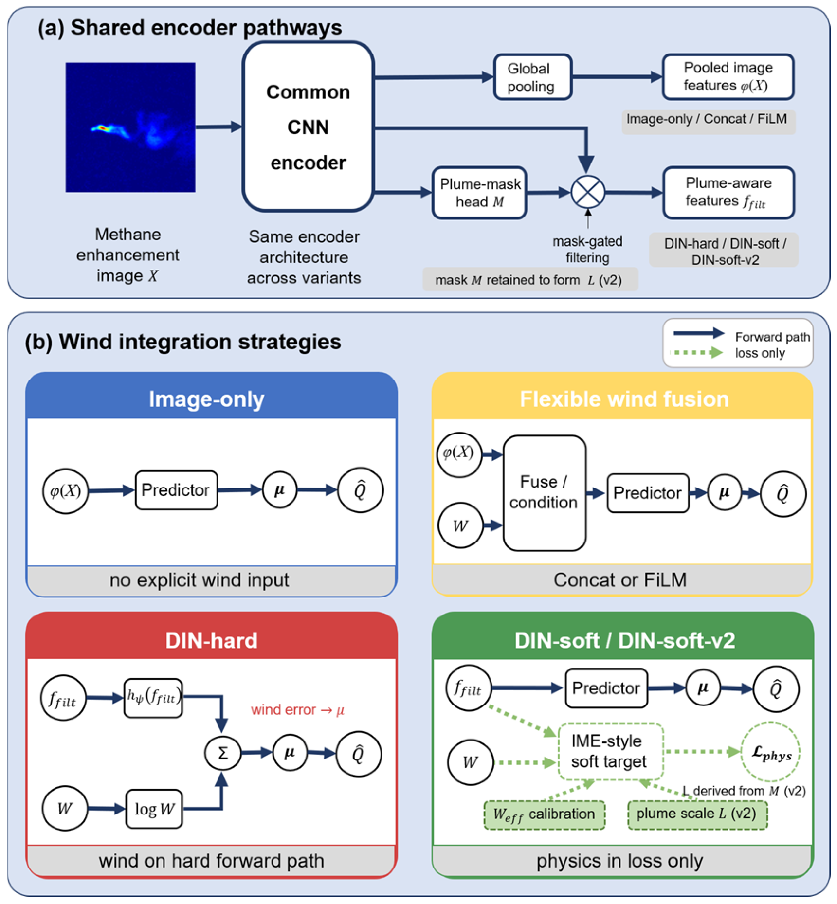
Figure 1 summarizes the comparison framework at the mechanism level. Panel (a) shows the shared encoder pathways and the DIN-specific plume-aware branch, and panel (b) contrasts the wind-integration strategies at the level of the predictive mean μ.

2.3. Backbone and Plume-Aware Representation

All DIN-style models use a shared convolutional encoder to extract a latent feature map f from the methane image. A detection branch, implemented in a U-Net-style encoder–decoder spirit [22], predicts a plume mask M, while a regression branch uses the latent representation for source-rate prediction. A key operation in the DIN family is spatial filtering, which suppresses background-dominated responses and emphasizes plume-relevant structure.

f_filt = f ⊙ M

(3)

The filtered feature map f_filt is pooled and passed to the source-rate head and, in the soft-physics models, to the branch that constructs the physical target. This design makes the physics guidance plume-aware rather than allowing it to act on arbitrary activations. For DIN-soft-v2, the predicted mask is additionally retained for the plume-scale term introduced in the generalized soft prior.

2.4. Wind-Integration Strategies

Two flexible wind-conditioning baselines are considered. In Concat, the pooled image feature φ(X) is concatenated with log W before regression. In FiLM [23], wind is used to generate feature-wise affine modulation parameters that condition the image representation before the final prediction head. These baselines establish the value of explicit wind usage without imposing a hard physical constraint.

z = [φ(X) ⊕ log W]

(4)

FiLM(f; W) = γ(W) ⊙ f + β(W)

(5)

2.4.1. Hard Physics-Coupled Variant (DIN-Hard)

DIN-hard is motivated by a simplified IME-inspired scaling relation in the log domain [10,11]. Classical IME formulations relate source rate to a plume-integrated mass enhancement, a transport velocity, and an effective plume length scale. Rather than treating this relation as a complete operational IME implementation, we use it only to motivate a controlled log-domain proxy. The schematic scaling can be written as follows.

Q = C₀ W IME/L

(6)

log Q = C + log W + log IME − log L

(7)

Here, C₀ is a proportionality coefficient and C = log C₀; IME and L denote the plume-mass and effective length-scale terms in the schematic IME relation. In DIN-hard, the log W term is placed directly on the forward path, whereas the remaining plume-mass and geometry information is represented by h_ψ(f_filt). Thus, DIN-hard is a simplified log-domain hard-coupling proxy rather than a full operational IME implementation.

μ = log W + h_ψ(f_filt)

(8)

This construction is interpretable as a controlled hard-coupling proxy, but it also imposes a strong structural assumption. Wind enters the output through a fixed global pathway with a unit coefficient, so wind error is transferred directly to the predictive mean. The comparison should therefore be read as a test of this simplified hard log-additive pathway rather than as a claim that all possible hard physical couplings are inferior.

To test whether the weakness of hard coupling is merely a consequence of fixing the wind coefficient to unity, an ablation is also considered in which the coefficient on log W is learned while wind remains on the hard forward path. This learnable hard-coupling variant is denoted DIN-k and is reported as an appendix ablation.

μ = k log W + h_ψ(f_filt)

(9)

2.4.2. Soft Physical-Guidance Variant (DIN-Soft)

DIN-soft relaxes the rigidity of DIN-hard by decoupling the main predictor from the physical relation. The log-mean is predicted through a flexible regression branch, while a plume-aware physical branch defines a soft auxiliary target.

μ = g_θ(X, W)

(10)

μ_phys = log W + h_ψ(f_filt)

(11)

$ℒ$_phys = ||μ − μ_phys||₂²

(12)

In this setting, the model can still benefit from physical structure, but it is no longer forced to satisfy the physical relation deterministically. When the physical proxy is informative, the regularizer encourages agreement. When the proxy is unreliable, the main predictor can deviate from it instead of inheriting the error directly.

2.4.3. Generalized Soft Prior (DIN-Soft-v2)

DIN-soft-v2 extends DIN-soft by introducing a generalized soft prior with a calibrated effective-wind proxy and a plume length-scale correction. The goal is to reduce approximation error in the auxiliary physical target while preserving a flexible forward predictor. These terms are used only in the auxiliary physical loss and should be understood as physics-inspired regularization terms rather than direct physical measurements.

μ_phys = c + k log W_eff + h_ψ(f_filt) − δ log L

(13)

The effective wind is not assumed to equal the raw scalar wind supplied to the network. Instead, it is learned through a calibration layer, W_eff = softplus(aW + b) + ε, where a and b are learned parameters and ε is a small positive constant. The resulting quantity should be read as a model-level transport proxy, not as a direct physical wind estimate.

W_eff = softplus(aW + b) + ε

(14)

The plume length-scale term is computed from the predicted soft plume mask. Specifically, the mask area is A = Σ_ij M_ij, and the length proxy is L = sqrt(A + A_min), with A_min used to avoid degeneracy for very small predicted masks. This heuristic is not intended as a precise geometric measurement; it is a compact, differentiable way to expose plume-extent information to the soft prior. Importantly, DIN-soft-v2 still does not hard-code the generalized physical relation into the forward prediction: the main predictor remains flexible, and the generalized IME expression appears only in the soft physical loss. The central advantage of soft guidance is therefore retained while the auxiliary physical target becomes less simplified.

2.5. Training Objective

All models are trained using a probabilistic log-domain objective, following standard heteroscedastic regression practice in deep learning [24]. Given the ground-truth source rate Q, the negative log-likelihood is defined as follows.

$ℒ$_NLL = 1/2 [log σ² + (log Q_gt − μ)²/σ²]

(15)

where the variance term is recovered from log σ² to ensure strict positivity during optimization.

For models equipped with a plume detection branch, an additional mask-supervision term $ℒ$_mask is used. For the soft physical-guidance models, the final training objective becomes

$ℒ$ = $ℒ$_NLL + λ_mask $ℒ$_mask + λ_phys $ℒ$_phys

(16)

This unified objective allows performance differences to be attributed mainly to wind integration and physics guidance rather than to unrelated changes in optimization. The learned variance term is used here as part of a stable probabilistic regression objective in the spirit of heteroscedastic uncertainty modeling [24]; the present experiments do not attempt a full calibration study of predictive intervals.

2.6. Dataset, Experimental Protocols, and Evaluation Metrics

All models are evaluated on a public LES-based methane plume benchmark derived from physically consistent numerical simulations. The benchmark complements earlier work on imaging-spectrometer detectability [9], IME-based quantification [10], PRISMA-based deep learning [16], and recent EnMAP/PRISMA source-rate estimation [17]. Each sample contains a background-subtracted methane column-enhancement image, an associated wind variable, and the ground-truth source rate. Plume fields and wind are generated within the same simulation framework, so the benchmark supports controlled perturbation experiments and relatively clean error attribution.

Each methane-enhancement sample is represented as a single-channel 100 × 100 image, and the source rate is treated as a scalar regression target. For models with plume-aware supervision, a continuous pseudo-plume-support mask is derived directly from the background-subtracted methane-enhancement field. The image-wise median is used as a background proxy, positive enhancement above that median is retained, and the resulting enhancement is normalized by the enhancement plus the image-wise standard deviation and a small ε. This produces a soft support map rather than an independent hand-labeled or physically exact plume boundary. No additional binary thresholding, morphological opening/closing, or connected-component cleanup is applied before using this continuous pseudo mask for auxiliary supervision or spatial diagnostics. The resulting mask is used only as weak auxiliary supervision for the detection branch and should therefore be interpreted as an approximate training prior. All comparisons follow the official benchmark train, validation, and test split, which also facilitates direct reproduction of the experiments.

All models are implemented in PyTorch and trained under a unified optimization protocol. Unless otherwise stated, training proceeds for 80 epochs using the AdamW optimizer with a cosine-annealing learning-rate schedule, gradient clipping, and a batch size of 32. This batch size was selected as a practical compromise between optimization stability, gradient-noise control, and GPU memory use for the shared 100 × 100 single-channel setting. No separate batch-size ablation was conducted, so the paper does not claim that 32 is universally optimal. The shared encoder, regression heads, and wind-integration modules are kept as consistent as possible across the model family so that observed differences can be attributed primarily to wind integration and physics guidance rather than arbitrary architectural changes. The experiments were run in Python 3.9.23 using PyTorch 2.8.0+cu128, torchvision 0.23.0+cu128, NumPy 1.24.4, SciPy 1.13.1, scikit-learn 1.6.1, pandas 2.3.3, and Matplotlib 3.9.4, with CUDA 12.8 on an NVIDIA GeForce RTX 5080 GPU.

The reported scalar metrics are coefficient of determination (R²), root mean squared error (RMSE), mean absolute error (MAE), and mean absolute percentage error (MAPE). R² and MAE are retained for completeness, whereas the main-text discussion emphasizes RMSE and MAPE. To assess plume-aware spatial consistency, center-of-mass shift (CMS) and plume alignment degree (PAD) are also reported. CMS is defined as the Euclidean displacement between the soft-mask centroids of the predicted plume mask and the pseudo-plume-support mask, measured in pixels. PAD is defined as the absolute difference between their second-moment principal-axis orientations, measured in degrees. The centroids and principal-axis orientations are computed from the continuous soft-mask weights using first- and second-order moments, rather than from a manually annotated plume boundary. For dispersed, broken, or multi-peak plumes, these moment-based diagnostics can be sensitive to the pseudo mask and should not be equated with true plume-boundary accuracy. They are therefore treated only as auxiliary indicators of plume-structure consistency rather than as substitutes for scalar inversion accuracy or manual segmentation validation. For the clean DIN-soft versus DIN-soft-v2 comparison,

Table A4. Bootstrap comparison between DIN-soft and DIN-soft-v2 on the clean overall test set (2000 resamples; 95% percentile confidence intervals).

Model	MAPE Bootstrap Mean [95% CI]	RMSE Bootstrap Mean [95% CI]
DIN-soft	6.42 [6.34, 6.51]	1375.41 [1350.08, 1400.94]
DIN-soft-v2	6.39 [6.31, 6.47]	1360.77 [1337.45, 1384.33]

reports bootstrap means and 95% confidence intervals from 2000 test-set resamples.

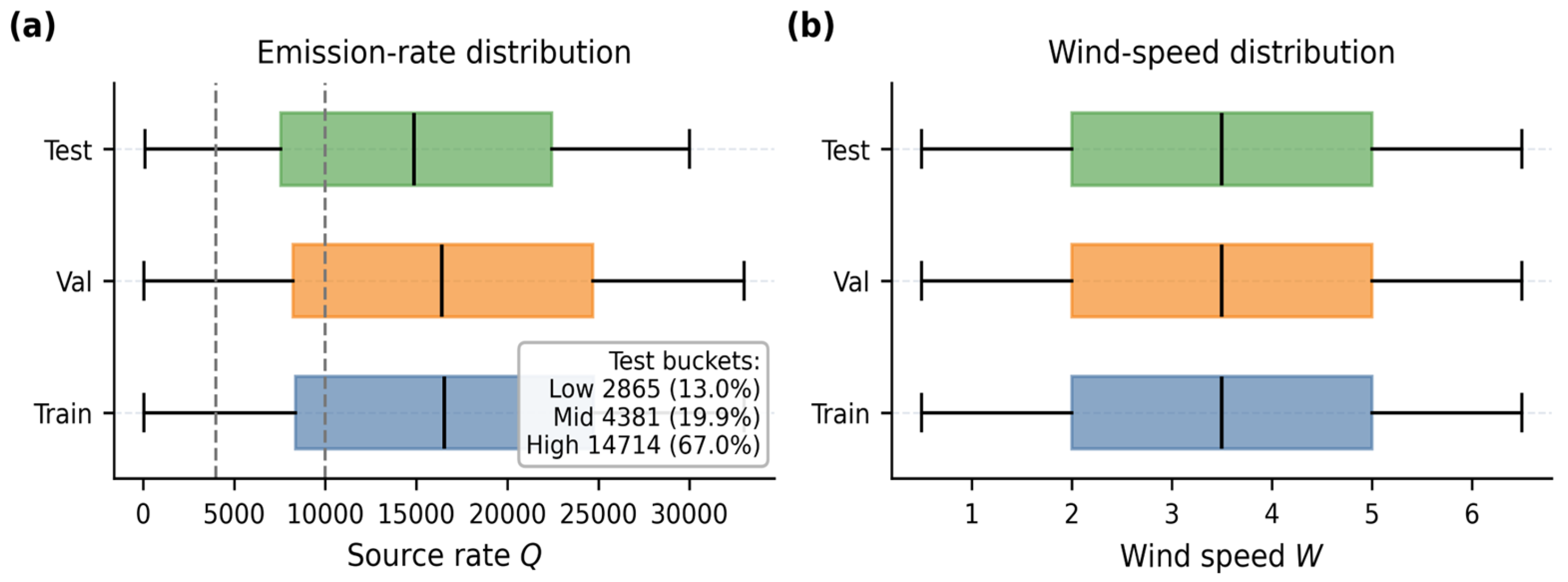
Overall metrics alone may obscure regime-dependent behavior because the test set is dominated by high-emission samples. A bucketed evaluation is therefore performed using three source-rate intervals: low (Q < 4000), mid (4000 ≤ Q < 10,000), and high (Q ≥ 10,000). In the test set, the low, mid, and high buckets contain 2865, 4381, and 14,714 samples, corresponding to 13.05%, 19.95%, and 67.00% of the test set, respectively. Because the high-emission bucket accounts for about two-thirds of the test samples, overall performance is interpreted together with bucketed results rather than in isolation. For regime-balanced comparison, an equal-weight macro-average across the three buckets is additionally reported in

Table A2. Equal-weight macro-average across low, mid, and high buckets. The arrows indicate the preferred direction of each metric (↓ lower is better).

Model	Macro RMSE ↓	Macro MAPE (%) ↓
Image-only	1069.02	10.24
Concat	784.21	6.92
FiLM	773.43	6.74
DIN-hard	1039.53	9.30
DIN-soft	798.00	7.06
DIN-soft-v2	795.00	7.02

.

Two complementary perturbation protocols are used to probe robustness to wind uncertainty. The first introduces deterministic multiplicative wind bias, W′ = αW, with α ∈ {0.7, 0.8, 0.9, 1.0, 1.1, 1.2, 1.3}. The second introduces multiplicative Gaussian wind noise, W′ = W(1 + ε), where ε ∼ N(0, σ_n²) and σ_n ∈ {0, 0.05, 0.10, 0.15, 0.20, 0.25, 0.30, 0.40}. For numerical stability, perturbed wind speeds are lower-bounded at 1 × 10⁻⁶ before the logarithm is taken. This implementation detail is important because extremely small perturbed winds can still create large negative log-wind values, especially for models with a hard log-additive wind pathway. For each noise level, the reported values are the mean and standard deviation across five independently sampled realizations. Absolute error curves are analyzed in tandem with relative degradation curves so that perturbation sensitivity can be separated from clean-condition baseline performance.

Several supplementary diagnostics were added to support the revision and are reported in Appendix A. First, a calibrated IME-style physical reference was constructed from the same train/test split. For each sample, the pseudo-plume support used for the spatial diagnostics was used to compute a pseudo-plume mass proxy P and a length-scale proxy L. Two forms were evaluated: a fixed proportional estimate Q_IME = c W P/L and a log-linear calibrated estimate log Q = a₀ + a₁ log W + a₂ log P − a₃ log L. The coefficients were fitted on the training split and then kept fixed for test evaluation.

This reference is an IME-style benchmark proxy, not a full operational IME implementation, because it uses the benchmark enhancement maps and pseudo-plume support rather than independently validated plume boundaries, full sensor-specific retrieval uncertainty, or plume-resolved winds.

Second, a positive-only log-normal wind perturbation, W′ = W exp(η), η ∼ N(−0.5σ², σ²), was used as a numerical diagnostic because it preserves positive wind speeds without lower-bound clipping. This diagnostic separates ordinary sensitivity to wind uncertainty from the extreme behavior that can occur when Gaussian perturbations produce near-zero winds in a log-wind pathway. Third, DIN-soft-v2 component ablations were added to isolate the roles of effective-wind calibration and the plume length-scale term.

Accordingly, Section 3 reports four matched experimental views: performance under clean conditions, robustness to deterministic wind bias, robustness to stochastic wind noise, and source-rate-stratified behavior across the low-, mid-, and high-emission regimes. Appendix A additionally reports the DIN-k ablation and the bootstrap comparison between DIN-soft and DIN-soft-v2.

3. Results

3.1. Performance Under Clean Conditions

Table 1. Clean overall comparison across all six model families. Higher R2 is better; lower values are better for all other metrics. The arrows indicate the preferred direction of each metric (↑ higher is better; ↓ lower is better). CMS is the plume-mask center-of-mass shift (pixels), and PAD is the principal-axis angular difference (degrees). CMS and PAD are reported only for plume-aware DIN models, and an em dash indicates that the metric is not applicable.

Model	R2 ↑	RMSE ↓	MAE ↓	MAPE (%) ↓	CMS ↓	PAD ↓
Image-only	0.957	1773.08	1235.95	9.03	—	—
Concat	0.976	1325.69	900.51	6.37	—	—
FiLM	0.976	1323.36	883.38	6.19	—	—
DIN-hard	0.958	1766.66	1192.08	8.44	4.09	2.84
DIN-soft	0.974	1375.54	910.08	6.42	4.07	2.72
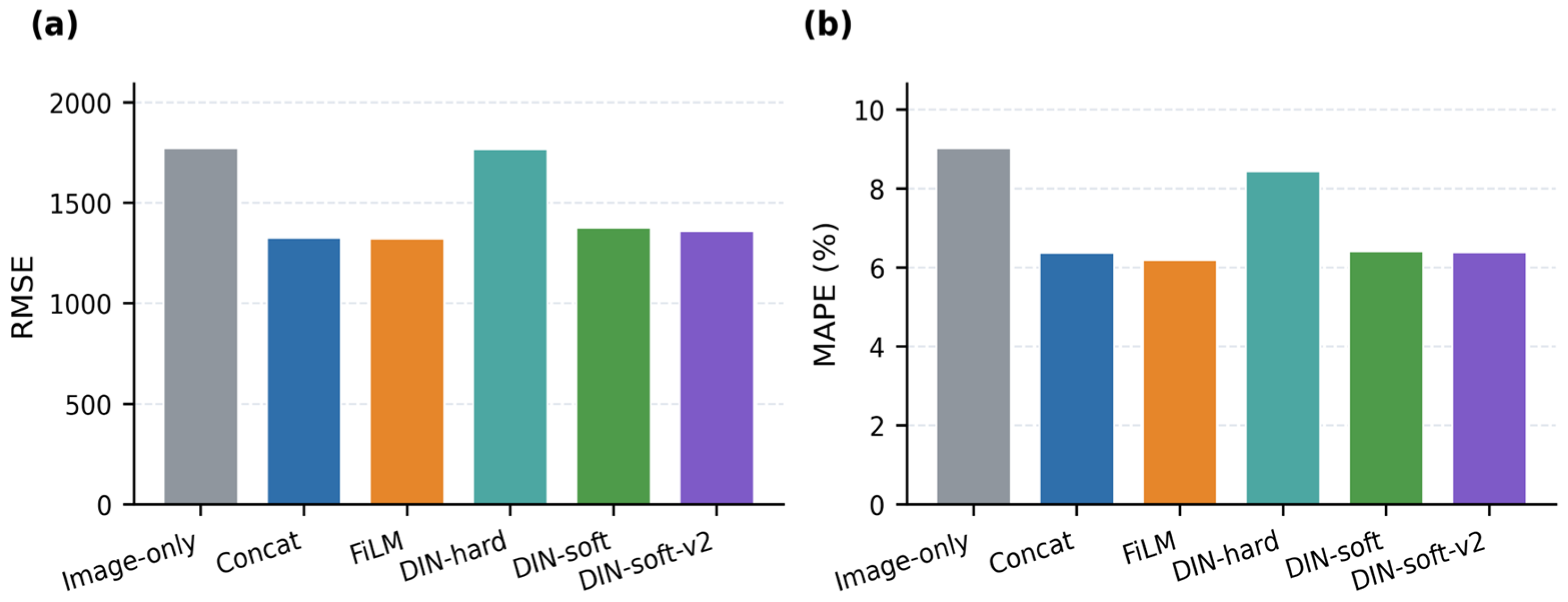
DIN-soft-v2	0.975	1360.94	903.63	6.39	3.92	2.60

and Figure 2 summarize clean-condition performance before any perturbation is introduced. Here, the clean condition refers to the benchmark reference setting with the original LES-derived wind input and no added deterministic bias or stochastic noise. The high-emission bucket contains 14,714 of the 21,960 test samples (about 67% of the test set), so overall metrics are informative but not sufficient on their own. Image-only does not use wind and therefore serves as a wind-invariant reference; its overall and bucketed values are repeated in

Table A1. Wind-invariant image-only references used for bias and noise comparisons. The arrows indicate the preferred direction of each metric (↓ lower is better).

Setting	RMSE ↓	MAPE (%) ↓
Overall	1773.08	9.03
Low bucket	310.02	13.89
Mid bucket	777.28	8.60
High bucket	2119.76	8.21

for the perturbation experiments.

Despite receiving the same wind input, DIN-hard trails the flexible baselines by a wide margin. Its overall RMSE is 1766.66, and its overall MAPE is 8.44%, clearly worse than both Concat and FiLM. The gap is therefore not explained by access to wind itself; it indicates that the simplified hard log-additive pathway already introduces structural mismatch under clean benchmark conditions.

Replacing hard coupling with soft physical guidance largely closes this gap. DIN-soft returns to the same general performance band as the strongest baselines, and DIN-soft-v2 improves slightly further in overall RMSE, MAPE, CMS, and PAD. The gain is modest, not transformative, so DIN-soft-v2 is better understood as the best-balanced physics-guided variant rather than as a new dominant scalar baseline over Concat or FiLM.

Table 2. Clean bucketed scalar performance (bucket counts: low = 2865, mid = 4381, high = 14,714). Lower values are better for all columns.

Model	Low RMSE	Low MAPE	Mid RMSE	Mid MAPE	High RMSE	High MAPE
Image-only	310.02	13.89	777.28	8.60	2119.76	8.21
Concat	195.52	8.62	570.06	6.13	1587.05	6.01
FiLM	190.85	8.50	542.28	5.87	1587.16	5.84
DIN-hard	258.27	11.86	743.61	8.16	2116.71	7.86
DIN-soft	190.34	9.24	552.65	5.94	1651.03	6.01
DIN-soft-v2	191.82	9.04	561.20	6.06	1631.97	5.97

reports clean bucketed scalar performance across the low-, mid-, and high-emission regimes. Because the high-emission bucket accounts for 67.00% of the test set, the bucketed and macro-average results are used to contextualize the overall scores in Table 1.

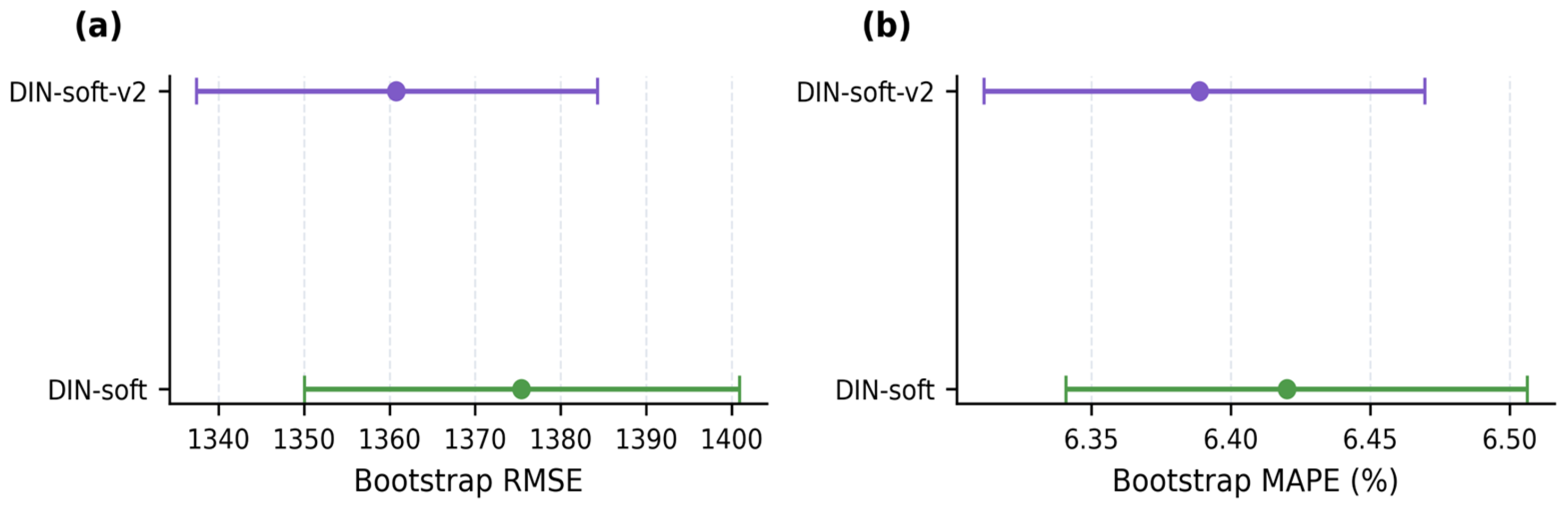
Bootstrap analysis with 2000 resamples was used to test whether the clean overall DIN-soft-v2 advantage persists under resampling. The bootstrap mean MAPE is 6.389 with a 95% CI of [6.312, 6.470] for DIN-soft-v2, compared with 6.420 [6.341, 6.506] for DIN-soft; the corresponding RMSE values are 1360.77 [1337.45, 1384.33] and 1375.41 [1350.08, 1400.94] (Table A4 and Figure A3). The intervals overlap, so the evidence supports a small but consistent improvement rather than a clearly separated effect.

The clean experiment supports three points within this benchmark. First, explicit wind input is helpful when it is fused flexibly. Second, the simplified hard forward coupling is not competitive even before the perturbation is introduced. Third, soft generalized physical guidance offers a better balance: predictive performance remains competitive, plume-aware spatial consistency improves modestly, and the clearest benefit appears in the high-emission regime.

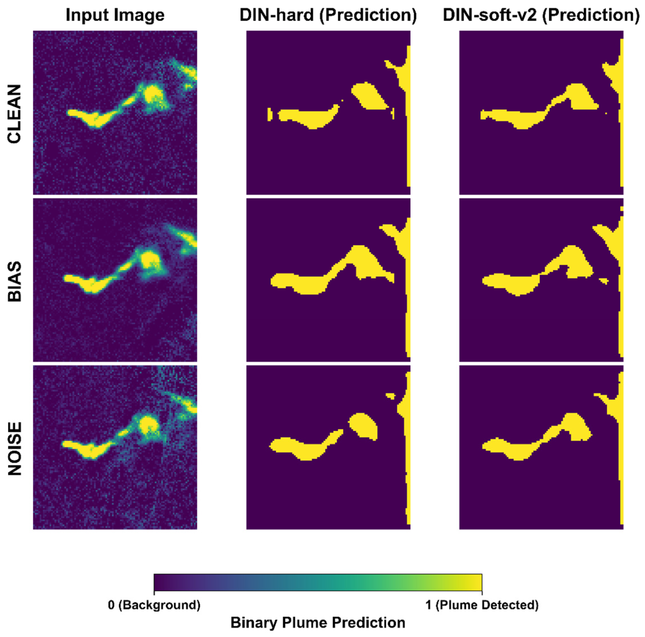
Figure 3 provides a qualitative comparison of binary plume predictions under representative clean, biased, and noisy conditions. This example is used only as a visual diagnostic of plume-mask coherence and is not a substitute for scalar source-rate accuracy.

3.2. Robustness to Deterministic Wind Bias

Table 3. Representative deterministic wind-bias response in the overall test set. Lower values are better for all columns.

Model	MAPE (α = 0.7)	MAPE (α = 1.0)	MAPE (α = 1.3)	RMSE (α = 0.7)	RMSE (α = 1.0)	RMSE (α = 1.3)
Concat	17.23	6.37	15.74	3155.90	1325.69	2980.62
FiLM	18.81	6.19	17.45	3518.32	1323.36	3356.05
DIN-hard	31.39	8.44	26.89	5480.54	1766.66	5167.89
DIN-soft	18.26	6.42	16.20	3379.34	1375.54	3088.83
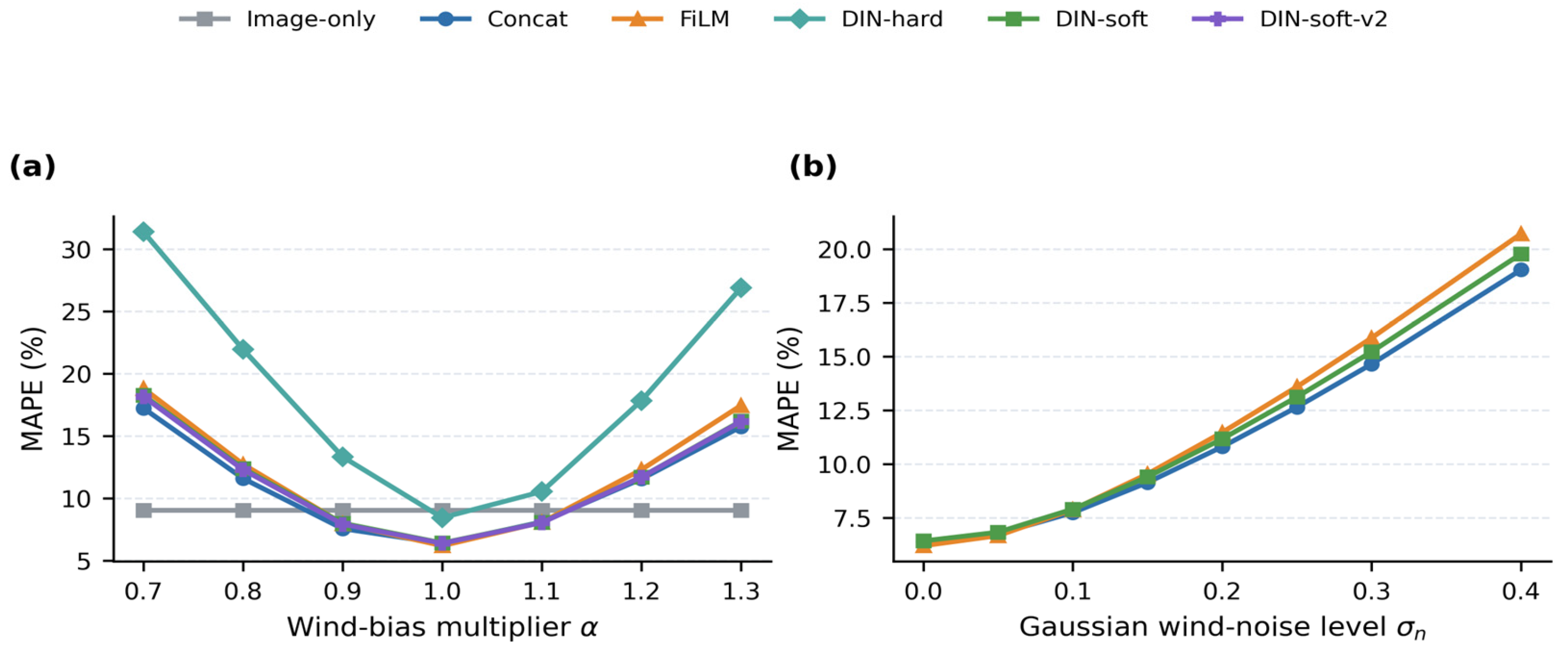
DIN-soft-v2	18.16	6.39	16.16	3367.80	1360.94	3059.87

and Figure 4 summarize the response to deterministic wind bias. To reduce visual density, Figure 4 focuses on overall MAPE trends, while RMSE values and bucket-level behavior are reported in the tables and Appendix A diagnostics.

DIN-hard shows the strongest bias sensitivity among the tested wind-using models. Its overall MAPE rises from 8.44% at α = 1.0 to 31.39% at α = 0.7 and 26.89% at α = 1.3. This increase is markedly steeper than for the flexible baselines and the soft-physics models, providing evidence that the simplified hard global coupling turns wind bias into a structural sensitivity channel.

Among the stable wind-using models, Concat is the strongest robustness baseline under deterministic bias. Its overall MAPE rises from 6.37% to 17.23% at α = 0.7 and 15.74% at α = 1.3, lower than the corresponding values for FiLM, DIN-soft, and DIN-soft-v2. The two soft-physics models nonetheless follow the same smooth-response pattern as the flexible baselines rather than the steep response of DIN-hard, showing that moving the physical relation from the forward structure into the loss substantially reduces sensitivity to systematic wind mismatch.

The DIN-soft versus DIN-soft-v2 comparison again shows limited but repeatable differences rather than a decisive separation. DIN-soft-v2 is slightly better overall and somewhat stronger in the high-emission bucket, whereas the low- and mid-emission buckets remain close. The deterministic-bias experiment therefore reinforces the main point of the paper: the issue is not whether wind is used, but whether it is injected through a rigid structural route.

3.3. Robustness to Stochastic Wind Noise

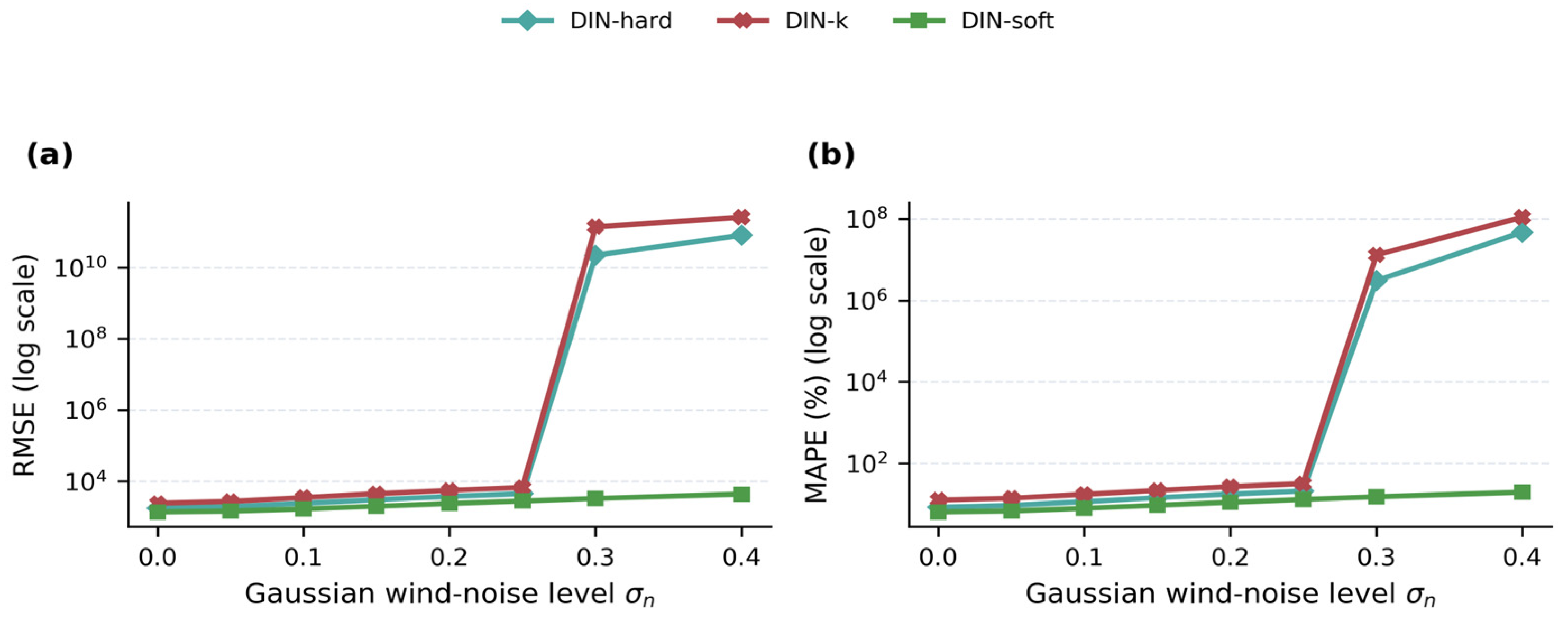
The contrast between the simplified hard pathway and soft physics guidance is clearest in the stochastic-noise experiment.

Table 4. Representative stochastic wind-noise response in the overall test set, reported as MAPE mean ± standard deviation. Lower values are better.

Model	MAPE (σn = 0.0)	MAPE (σn = 0.1)	MAPE (σn = 0.2)	MAPE (σn = 0.3)	MAPE (σn = 0.4)
Concat	6.37 ± 0.00	7.73 ± 0.02	10.80 ± 0.04	14.65 ± 0.05	19.03 ± 0.10
FiLM	6.19 ± 0.00	7.87 ± 0.03	11.47 ± 0.04	15.86 ± 0.05	20.71 ± 0.09
DIN-hard	8.44 ± 0.00	11.56 ± 0.03	17.72 ± 0.04	3.08 × 106 ± 1.33 × 106	4.69 × 107 ± 7.48 × 106
DIN-soft	6.42 ± 0.00	7.90 ± 0.04	11.16 ± 0.06	15.22 ± 0.07	19.78 ± 0.12
DIN-soft-v2	6.39 ± 0.00	7.86 ± 0.03	11.11 ± 0.05	15.14 ± 0.07	19.69 ± 0.12

and Figure A2 show that DIN-hard becomes numerically unstable at higher noise levels under the implemented Gaussian wind-noise protocol, while Figure 4b summarizes the stable-model MAPE trends on linear axes. Its overall MAPE rises from 17.72% at σ_n = 0.2 to 3.08 × 10⁶% at σ_n = 0.3 and 4.69 × 10⁷% at σ_n = 0.4, indicating extreme sensitivity rather than ordinary accuracy degradation. RMSE shows the same pattern, increasing to 2.23 × 10¹⁰ at σ_n = 0.3 and continuing to diverge at σ_n = 0.4. These perturbations are imposed only during evaluation of already trained models, so the extreme values should be interpreted as inference-time sensitivity of the log-wind forward pathway rather than as training-time gradient explosion.

The learnable hard-coupling ablation DIN-k does not remove this failure mode under the same perturbation protocol. As summarized in

Table A3. Learnable hard-coupling ablation under stochastic wind noise. Entries report values at σ_n = 0, 0.2, and 0.3 together with the fitted wind-coupling coefficient.

Model	Wind Coupling	MAPE (%) at σn = {0, 0.2, 0.3}	RMSE at σn = {0, 0.2, 0.3}
DIN-hard	fixed 1.000	8.44/17.72/3.08 × 106	1766.66/3774.15/2.23 × 1010
DIN-k	learned 1.471	12.68/26.91/1.32 × 107	2428.87/5611.70/1.39 × 1011

and illustrated in Figure A2, DIN-k is already worse than DIN-hard under clean conditions (MAPE 12.68% vs. 8.44%; RMSE 2428.87 vs. 1766.66) and degrades even faster under noise (MAPE 26.91% vs. 17.72% at σ_n = 0.2). This ablation argues against treating DIN-hard as a strawman within the present simplified hard-coupling family: relaxing the scalar wind coefficient alone does not make the hard forward path robust.

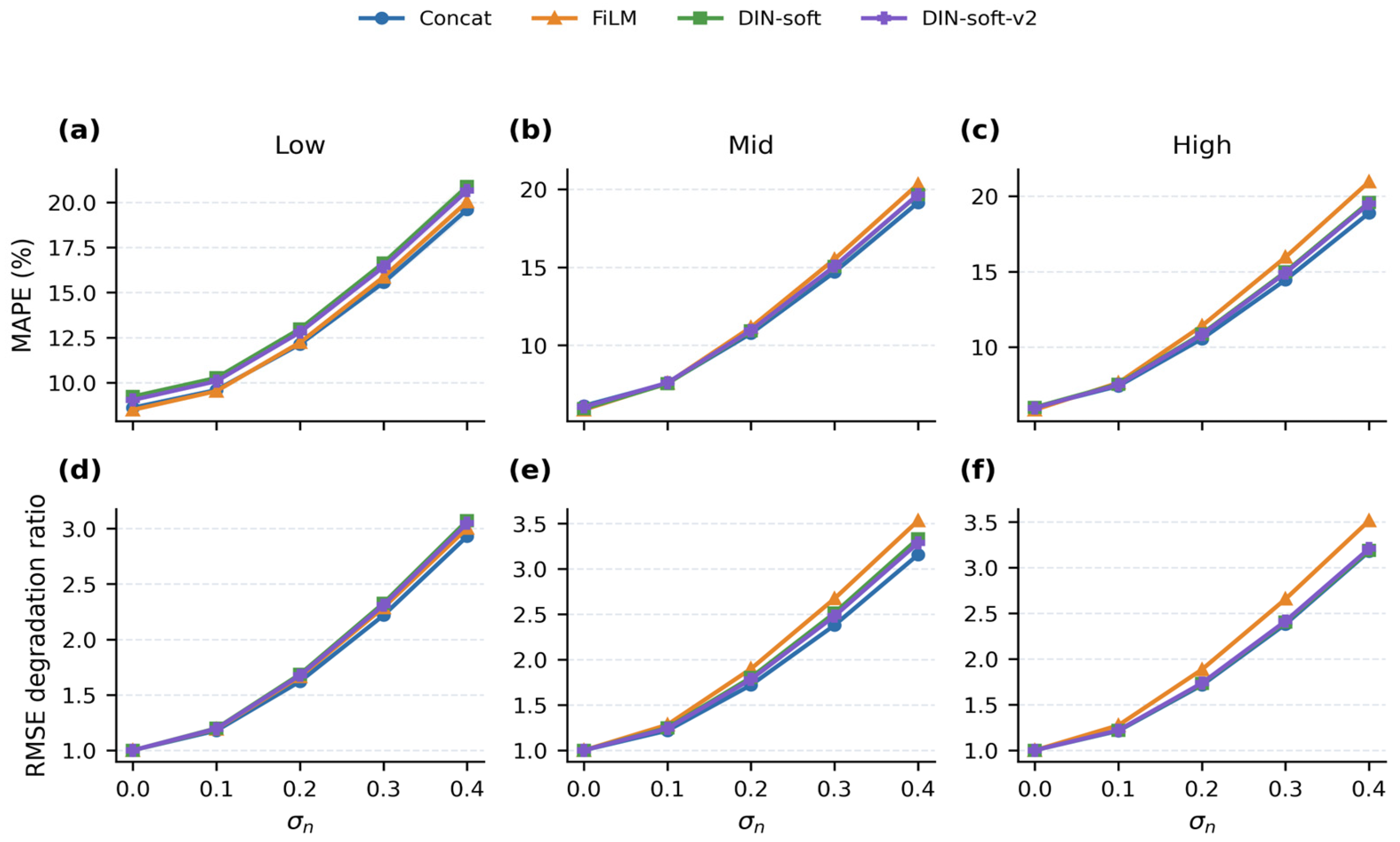
Figure 4 summarizes the main overall MAPE robustness trends, and Figure A2 shows the hard-coupling behavior on log scales. Figure A1 provides the bucketed wind-noise and relative-degradation diagnostics.

The bucketed noise curves offer a more nuanced view. In the low-emission bucket, DIN-soft-v2 improves only slightly over DIN-soft and still trails the strongest flexible baselines. In the mid-emission bucket, DIN-soft and DIN-soft-v2 are nearly indistinguishable in scalar error. However, in the high-emission bucket, DIN-soft-v2 consistently improves on DIN-soft at all reported noise levels and remains relatively close to Concat. Within this benchmark, the main benefit of the generalized IME soft prior is therefore concentrated in the high-emission regime rather than being uniform across all operating conditions.

For readability, the main text reports the simplified overall MAPE robustness view in Figure 4, whereas the more detailed bucketed degradation and log-scale hard-coupling diagnostics are deferred to Figure A1 and Figure A2.

3.4. Learned Soft-Prior Parameters and Cross-Setting Summary

Table 5. Learned parameters of the DIN-soft-v2 soft prior.

Model	k	δ	a	b	c
DIN-soft-v2	1.515	0.088	1.769	3.523	2.387

lists the learned parameters that define the DIN-soft-v2 soft prior. They should not be interpreted as physical constants, because they are fitted within a data-driven model and depend on dataset scaling and implementation details. They remain diagnostically useful. In particular, the wind-calibration parameters show that the model does not simply reuse the raw wind input as the effective transport velocity; instead, it learns a nontrivial calibration before wind enters the soft physical target. This again suggests that the transport quantity useful to an IME-like relation need not coincide with the externally supplied scalar wind.

The learned coefficient for the length-scale correction is comparatively small (0.088). This suggests that the shared convolutional encoder already captures much of the relevant plume geometry in its latent representation, so the explicit L term is complementary rather than dominant.

Across clean, biased, noisy, and bucketed evaluations, the same benchmark-level pattern recurs. Wind information is helpful when it is fused flexibly. The weakness of DIN-hard lies not in the use of physics itself, but in the rigidity of the simplified hard global coupling, which turns wind error into a direct failure path. Soft physical guidance offers a more reliable alternative within the tested setting: it recovers competitive predictive performance without numerical collapse under the reported perturbations. DIN-soft-v2 adds modest gains over DIN-soft, with the clearest benefit in the high-emission regime and in plume spatial consistency.

3.5. Additional Physical Baseline, Positive-Wind Diagnostic, and Soft-Prior Ablation

The first revision experiment adds a calibrated IME-style baseline as a non-neural physical reference (

Table A5. Calibrated IME-style physical baseline under clean, deterministic-bias, and Gaussian-noise settings. The calibrated form is fitted on the training split and evaluated on the same test split as the neural models.

Model	Clean RMSE	Clean MAPE	Bias MAPE Range	Gaussian MAPE (σ = 0.4)
IME-fixed	5435.48	54.11	48.72–79.92	69.16
IME-calibrated	3245.71	24.45	24.45–26.39	27.45

). The fixed proportional form is deliberately simple, and the log-linear calibrated form is fitted only on the training split, so this comparison should be read as an IME-style reference under the benchmark proxies rather than as a full operational IME retrieval. Calibration reduces clean MAPE from 54.11% to 24.45%, but the calibrated physical reference remains less accurate than the learning-based models.

The second revision experiment adds a positive-only log-normal wind-noise diagnostic (

Table A6. Positive-only log-normal wind-noise diagnostic for the main neural models. This perturbation preserves strictly positive wind speed and is used to separate ordinary wind sensitivity from clipping-induced near-zero wind effects.

Model	MAPE (σ = 0.0)	MAPE (σ = 0.2)	MAPE (σ = 0.3)	MAPE (σ = 0.4)
Concat	6.37	10.68	14.26	18.05
FiLM	6.19	11.41	15.61	20.07
DIN-hard	8.44	17.84	24.89	32.18
DIN-soft	6.42	11.09	14.89	18.91
DIN-soft-v2	6.39	11.03	14.81	18.81
DIN-k	12.68	27.03	38.03	49.72

and

Table A8. Wind-perturbation diagnostics for Gaussian and log-normal protocols. Fractions are reported relative to the test set.

Protocol	σ	Min Wind	Non-Positive (%)	Below 10−3 (%)
Gaussian before clip	0.3	−1.679	0.041	0.041
Gaussian after clip	0.3	0.000001	0.000	0.041
Log-normal	0.3	0.175	0.000	0.000
Gaussian before clip	0.4	−4.005	0.600	0.605
Gaussian after clip	0.4	0.000001	0.000	0.605
Log-normal	0.4	0.121	0.000	0.000

) to separate ordinary wind sensitivity from numerical effects introduced by near-zero clipped Gaussian winds. Under Gaussian perturbations, a small fraction of σ = 0.3 and σ = 0.4 winds become non-positive before clipping; under log-normal perturbations, all wind values remain positive. In the positive-only protocol, DIN-hard no longer exhibits the extreme Gaussian blow-up, but it remains more sensitive than the flexible and soft-guidance models.

The third revision experiment reports the DIN-soft-v2 component ablation (

Table A7. DIN-soft-v2 component ablation. The table compares the full DIN-soft-v2 model with variants removing the learned effective-wind calibration or the plume length-scale term.

Model	Clean RMSE	Clean MAPE	CMS	PAD	Log-Normal MAPE (σ = 0.3)
Full model	1360.94	6.39	3.92	2.60	14.81
w/o W_eff	1359.58	6.38	3.81	2.70	14.88
w/o L	1359.83	6.40	3.71	2.65	14.98

). Removing the effective-wind calibration or the length-scale term changes the clean and log-normal-noise scores only slightly. These results indicate that W_eff and L act as small auxiliary refinements, whereas the main robustness difference in this benchmark comes from using the IME-inspired relation as a soft regularizer rather than as the simplified hard forward pathway.

4. Discussion

4.1. Positioning Within Methane Quantification Pipelines

Conventional methane quantification pipelines estimate emission rates from plume mass and transport using IME [10,11] or related flux formulations [1,7,12]. Recent studies have also developed learning-based methods for PRISMA [16], EnMAP/PRISMA [17], automated satellite monitoring [18,19], and controlled-release or single-blind validation across satellite systems [20,21]. Those studies establish that methane-plume imagery can support detection and, in some cases, source-rate estimation, but they do not explicitly compare hard forward IME coupling against soft physics regularization under controlled wind perturbations. The present study sits between these strands. It does not propose a new sensor-specific detector; instead, it isolates how wind should be integrated when the task is source-rate regression.

That positioning matters because wind is both necessary and imperfectly observed. In methane studies, wind often comes from ancillary meteorological products rather than plume-scale measurements [1,12,13]. Its representativeness in space, time, and height can be limited [14,15], and IME-based inversion is known to be sensitive to such a mismatch [10]. Existing deep-learning quantification studies [8,16,17] generally treat wind as helpful context, whereas classic IME studies [10,11,12] make the wind dependence explicit. This paper contributes by comparing those design choices within one matched benchmark rather than by claiming a new general best model.

The controlled model family separates three questions that are often mixed together: whether wind should be used at all, whether it should modulate learned features or enter an explicit equation, and whether an IME-inspired relation should act as a hard pathway or as a soft prior. The contribution is therefore mainly methodological and empirical rather than a claim of a universally superior model. Relative to prior methane-learning studies, the key novelty is the controlled comparison itself and the resulting benchmark-level design evidence about how to integrate uncertain auxiliary physics.

Within the present benchmark, the answer is consistent but should be interpreted cautiously. Image-only regression provides a wind-invariant reference, flexible fusion provides the strongest scalar baseline, and the tested physics-guided variants are useful only when the IME-inspired structure is introduced softly rather than rigidly. Because the benchmark emulates EnMAP/PRISMA-style stand-off imaging spectroscopy, this conclusion is most directly relevant as a controlled design lesson for airborne and satellite workflows and should not be read as direct evidence of field-ready performance.

4.2. Mechanistic Interpretation of Hard Coupling and Soft Physical Guidance

The weakness of DIN-hard is not just a lower score; it points to a specific sensitivity mechanism of the simplified hard formulation. In this formulation, the predictive mean is forced through a log-additive wind pathway, so bias or noise in W is transferred directly to the output. That pathway cannot be selectively attenuated, so the model is structurally required to trust wind even when the supplied value is wrong. Under the Gaussian noise protocol, very small lower-bounded wind values can further amplify this sensitivity through the logarithm.

The learnable hard-coupling ablation sharpens this point. If the issue were only the choice of a fixed coefficient, then allowing the coefficient to adapt should have mitigated the failure. It does not. DIN-k learns a coefficient of about 1.471, which indicates over-amplification rather than self-suppression, and the model remains even more fragile under noise. The problem is therefore the hard forward route itself, not merely the numerical value attached to it.

This interpretation is consistent with broader discussions in physics-informed machine learning [25], deep learning and process understanding for data-driven Earth system science [26], and scientific-knowledge integration frameworks [27]: more explicit physics does not automatically improve robustness. When the auxiliary variable carrying that physics is uncertain, the model must be able to discount or reinterpret it.

Physical interpretability and architectural rigidity are therefore not the same thing. A model may look more physical on paper yet be less reliable in deployment if its physical node is poorly matched to how uncertainty enters the problem.

4.3. Interpreting the Soft Prior as Representation Regularization

DIN-soft and DIN-soft-v2 suggest a different role for physics. Once the IME-like relation is moved from the forward equation into a loss term, the model can still learn plume-aware representations while avoiding deterministic error propagation. In practice, the soft prior acts as a representation-level regularizer: it nudges the network toward transport-consistent structure without forcing every prediction to obey a possibly mis-specified wind value.

This interpretation helps explain why the soft models remain stable under both bias and noise. The plume-aware branch still encourages geometric consistency, and the physical loss still rewards agreement with an IME-like target, but the predictor can deviate when that target becomes unreliable. The result is smooth degradation rather than catastrophic failure.

DIN-soft-v2 adds two refinements to this regularization view: a calibrated effective wind and a plume length-scale term. The bootstrap comparison consistently favors DIN-soft-v2, but only by a modest margin. That result is informative in itself: improving the prior helps, yet the main gain comes from moving from hard coupling to soft guidance, not from increasingly elaborate parameterization.

The regime dependence is equally informative. The clearest DIN-soft-v2 gains appear in the high-emission bucket, where plume structure is strong enough for the generalized prior to matter. In the low-emission bucket, plume morphology is weaker and more ambiguous, so even a better prior cannot fully close the gap to the strongest flexible baselines. The soft prior is therefore most useful as structured regularization when the plume signal is already reasonably expressed.

4.4. Practical Implications for Robust Methane Inversion

For operational methane monitoring, the present benchmark-level design lesson is relevant but not sufficient by itself. Satellite and airborne observations used in super-emitter surveys and validation campaigns face retrieval residuals, background heterogeneity, striping noise, geolocation mismatch, spectral artifacts, and wind representativeness errors that are not fully reproduced by the LES benchmark. A deployable inversion model should therefore treat wind as informative context rather than as an unquestioned oracle, but real-scene validation remains necessary before operational use.

The DIN-soft family is therefore best understood as a physically grounded alternative within this controlled benchmark rather than as a uniformly superior scalar regressor. On this benchmark, flexible baselines such as Concat and FiLM attain slightly better scalar accuracy in several settings. The value of the soft-physics designs lies elsewhere: they encourage plume-consistent structure and preserve an interpretable IME-inspired regularization pathway without forcing the prediction through the simplified hard forward equation. Whether that trade-off remains beneficial for real satellite scenes or airborne stand-off measurements requires recalibration, transfer learning, or domain-adaptation verification.

4.5. Limitations and Future Work

The present conclusions are established on a public LES-based synthetic benchmark rather than on raw real-world EnMAP, PRISMA, GF-5, EMIT, or MethaneAIR scenes. This choice is methodologically useful because it enables matched experiments under controlled wind perturbations, but it does not remove the simulation-to-reality gap. Real scenes add matched-filtering and retrieval residuals, nonlinear spectral-inversion errors, surface and background complexity [14,15], clouds or artifacts, geolocation uncertainty, instrument noise, and validation challenges that can only be resolved with observational studies [20,21], sim-to-real adaptation methods [28], and satellite-based surveys of extreme methane emissions [29,30].

Accordingly, the present claims should be read as comparative design conclusions within a controlled benchmark, not as final statements about field-ready performance. Four limitations are especially important. First, the study is benchmark-based and does not yet include raw real-scene or controlled-release validation. Second, the meteorological input is represented by a single scalar wind variable rather than by a richer transport description. Third, although the models are trained with a probabilistic objective, the paper does not provide a dedicated calibration analysis of predictive intervals. Fourth, the comparison remains centered on a matched model family; the added calibrated IME-style baseline provides a physical reference, but broader external neural baselines and operational processing chains remain outside the present scope. The most direct next steps are real-scene transfer, controlled-release validation [20,21], observational cross-checks with airborne data [8], richer wind representations, external baseline comparison, and domain-adaptation methods for remote sensing [28].

5. Conclusions

This study was designed as a controlled benchmark test of how uncertain wind information should enter learning-based methane source-rate inversion from plume imagery. Three findings emerge from the clean, biased-wind, stochastic-noise, bucketed, and supplementary diagnostic experiments. First, wind information is useful, but the integration strategy matters: flexible wind conditioning gives the strongest clean scalar baselines, while the image-only model remains a necessary wind-invariant reference for separating plume-morphology information from explicit wind usage.

Second, the simplified hard log-additive pathway tested here is the main source of fragility. DIN-hard is already less competitive than Concat and FiLM under clean inputs, degrades steeply under deterministic wind bias, and becomes extremely sensitive under the Gaussian wind-noise protocol when near-zero clipped winds enter the log-wind pathway. The DIN-k ablation and the positive-only log-normal diagnostic further show that learning a scalar wind coefficient or avoiding non-positive winds reduces neither the general sensitivity nor the need to interpret the Gaussian blow-up cautiously.

Third, soft physical guidance changes the failure mode rather than simply maximizing every scalar metric. DIN-soft and DIN-soft-v2 remain stable under the reported perturbations, and DIN-soft-v2 provides modest improvements over DIN-soft, mainly in the high-emission regime and in plume-aware spatial consistency. The component ablations indicate that the effective-wind calibration and plume length-scale term act as auxiliary refinements; the broader design implication is that, within this LES benchmark, an IME-inspired relation is safer as a calibratable regularizer than as the simplified hard forward constraint tested here. This conclusion should be treated as benchmark-level evidence, and its real-scene value still needs validation with raw satellite or airborne observations, controlled-release experiments, richer wind information, and domain-adaptation or transfer-learning workflows.

References

1. Jacob, D.J.; Varon, D.J.; Cusworth, D.H.; Dennison, P.E.; Frankenberg, C.; Gautam, R.; Guanter, L.; Kelley, J.; McKeever, J.; Ott, L.E.; et al. Quantifying methane emissions from the global scale down to point sources using satellite observations of atmospheric methane. Atmos. Chem. Phys. 2022, 22, 9617–9646. [Google Scholar] [CrossRef]
2. Saunois, M.; Stavert, A.R.; Poulter, B.; Bousquet, P.; Canadell, J.G.; Jackson, R.B.; Raymond, P.A.; Dlugokencky, E.J.; Houweling, S.; Patra, P.K.; et al. The Global Methane Budget 2000–2017. Earth Syst. Sci. Data 2020, 12, 1561–1623. [Google Scholar] [CrossRef]
3. Alvarez, R.A.; Zavala-Araiza, D.; Lyon, D.R.; Allen, D.T.; Barkley, Z.R.; Brandt, A.R.; Davis, K.J.; Herndon, S.C.; Jacob, D.J.; Karion, A.; et al. Assessment of methane emissions from the U.S. oil and gas supply chain. Science 2018, 361, 186–188. [Google Scholar] [CrossRef] [PubMed]
4. Sherwin, E.D.; Rutherford, J.S.; Zhang, Z.; Chen, Y.; Wetherley, E.B.; Yakovlev, P.V.; Berman, E.S.F.; Jones, B.B.; Cusworth, D.H.; Thorpe, A.K.; et al. US oil and gas system emissions from nearly one million aerial site measurements. Nature 2024, 627, 328–334. [Google Scholar] [CrossRef] [PubMed]
5. Guanter, L.; Irakulis-Loitxate, I.; Gorroño, J.; Sánchez-García, E.; Cusworth, D.H.; Varon, D.J.; Cogliati, S.; Colombo, R. Mapping methane point emissions with the PRISMA spaceborne imaging spectrometer. Remote Sens. Environ. 2021, 265, 112671. [Google Scholar] [CrossRef]
6. Chabrillat, S.; Foerster, S.; Segl, K.; Beamish, A.; Brell, M.; Asadzadeh, S.; Milewski, R.; Ward, K.J.; Brosinsky, A.; Koch, K.; et al. The EnMAP spaceborne imaging spectroscopy mission: Initial scientific results two years after launch. Remote Sens. Environ. 2024, 315, 114379. [Google Scholar] [CrossRef]
7. Thorpe, A.K.; Frankenberg, C.; Aubrey, A.; Roberts, D.; Nottrott, A.; Rahn, T.; Sauer, J.; Dubey, M.; Costigan, K.; Arata, C.; et al. Mapping methane concentrations from a controlled release experiment using the next generation airborne visible/infrared imaging spectrometer (AVIRIS-NG). Remote Sens. Environ. 2016, 179, 104–115. [Google Scholar] [CrossRef]
8. Guanter, L.; Warren, J.; Omara, M.; Chulakadabba, A.; Roger, J.; Sargent, M.; Franklin, J.E.; Wofsy, S.C.; Gautam, R. Detection and quantification of methane plumes with the MethaneAIR airborne spectrometer. Atmos. Meas. Tech. 2025, 18, 3857–3872. [Google Scholar] [CrossRef]
9. Cusworth, D.H.; Jacob, D.J.; Varon, D.J.; Miller, C.C.; Liu, X.; Chance, K.; Thorpe, A.K.; Duren, R.M.; Miller, C.E.; Thompson, D.R.; et al. Potential of next-generation imaging spectrometers to detect and quantify methane point sources from space. Atmos. Meas. Tech. 2019, 12, 5655–5668. [Google Scholar] [CrossRef]
10. Varon, D.J.; Jacob, D.J.; McKeever, J.; Jervis, D.; Durak, B.O.A.; Xia, Y.; Huang, Y. Quantifying methane point sources from fine-scale satellite observations of atmospheric methane plumes. Atmos. Meas. Tech. 2018, 11, 5673–5686. [Google Scholar] [CrossRef]
11. Jongaramrungruang, S.; Frankenberg, C.; Matheou, G.; Thorpe, A.K.; Thompson, D.R.; Kuai, L.; Duren, R.M. Towards accurate methane point-source quantification from high-resolution 2-D plume imagery. Atmos. Meas. Tech. 2019, 12, 6667–6681. [Google Scholar] [CrossRef]
12. Gorroño, J.; Varon, D.J.; Irakulis-Loitxate, I.; Guanter, L. Understanding the potential of Sentinel-2 for monitoring methane point emissions. Atmos. Meas. Tech. 2023, 16, 89–107. [Google Scholar] [CrossRef]
13. Varon, D.J.; Jervis, D.; McKeever, J.; Spence, I.; Gains, D.; Jacob, D.J. High-frequency monitoring of anomalous methane point sources with multispectral Sentinel-2 satellite observations. Atmos. Meas. Tech. 2021, 14, 2771–2785. [Google Scholar] [CrossRef]
14. Bhardwaj, P.; Kumar, R.; Mitchell, D.A.; Randles, C.A.; Downey, N.; Blewitt, D.; Kosovic, B. Evaluating the detectability of methane point sources from satellite observing systems using microscale modeling. Sci. Rep. 2022, 12, 17425. [Google Scholar] [CrossRef] [PubMed]
15. Ayasse, A.K.; Thorpe, A.K.; Roberts, D.A.; Funk, C.C.; Dennison, P.E.; Frankenberg, C.; Steffke, A.; Aubrey, A.D. Evaluating the effects of surface properties on methane retrievals using a synthetic airborne visible/infrared imaging spectrometer next generation (AVIRIS-NG) image. Remote Sens. Environ. 2018, 215, 386–397. [Google Scholar] [CrossRef]
16. Joyce, P.; Villena, C.R.; Huang, Y.; Webb, A.; Gloor, M.; Wagner, F.H.; Chipperfield, M.P.; Guilló, R.B.; Wilson, C.; Boesch, H. Using a deep neural network to detect methane point sources and quantify emissions from PRISMA hyperspectral satellite images. Atmos. Meas. Tech. 2023, 16, 2627–2640. [Google Scholar] [CrossRef]
17. Ouerghi, E.; Ehret, T.; Facciolo, G.; Meinhardt, E.; Marion, R.; Morel, J.-M. Tightening up methane plume source rate estimation in EnMAP and PRISMA images. Atmos. Meas. Tech. 2025, 18, 4611–4629. [Google Scholar] [CrossRef]
18. Schuit, B.J.; Maasakkers, J.D.; Bijl, P.; Mahapatra, G.; Berg, A.-W.v.D.; Pandey, S.; Lorente, A.; Borsdorff, T.; Houweling, S.; Varon, D.J.; et al. Automated detection and monitoring of methane super-emitters using satellite data. Atmos. Chem. Phys. 2023, 23, 9071–9098. [Google Scholar] [CrossRef]
19. Vaughan, A.; Mateo-García, G.; Gómez-Chova, L.; Růžička, V.; Guanter, L.; Irakulis-Loitxate, I. CH4Net: A deep learning model for monitoring methane super-emitters with Sentinel-2 imagery. Atmos. Meas. Tech. 2024, 17, 2583–2593. [Google Scholar] [CrossRef]
20. Sherwin, E.D.; Rutherford, J.S.; Chen, Y.; Aminfard, S.; Kort, E.A.; Jackson, R.B.; Brandt, A.R. Single-blind validation of space-based point-source detection and quantification of onshore methane emissions. Sci. Rep. 2023, 13, 3836. [Google Scholar] [CrossRef] [PubMed]
21. Sherwin, E.D.; El Abbadi, S.H.; Burdeau, P.M.; Zhang, Z.; Chen, Z.; Rutherford, J.S.; Chen, Y.; Brandt, A.R. Single-blind test of nine methane-sensing satellite systems from three continents. Atmos. Meas. Tech. 2024, 17, 765–782. [Google Scholar] [CrossRef]
22. Ronneberger, O.; Fischer, P.; Brox, T. U-Net: Convolutional networks for biomedical image segmentation. In Medical Image Computing and Computer-Assisted Intervention—MICCAI 2015; Springer: Cham, Switzerland, 2015; Volume 9351, pp. 234–241. [Google Scholar] [CrossRef]
23. Perez, E.; Strub, F.; De Vries, H.; Dumoulin, V.; Courville, A. FiLM: Visual reasoning with a general conditioning layer. Proc. AAAI Conf. Artif. Intell. 2018, 32, 3942–3951. [Google Scholar] [CrossRef]
24. Kendall, A.; Gal, Y. What uncertainties do we need in Bayesian deep learning for computer vision? Adv. Neural Inf. Process. Syst. 2017, 30, 5574–5584. [Google Scholar]
25. Karniadakis, G.E.; Kevrekidis, I.G.; Lu, L.; Perdikaris, P.; Wang, S.; Yang, L. Physics-informed machine learning. Nat. Rev. Phys. 2021, 3, 422–440. [Google Scholar] [CrossRef]
26. Reichstein, M.; Camps-Valls, G.; Stevens, B.; Jung, M.; Denzler, J.; Carvalhais, N.; Prabhat. Deep learning and process understanding for data-driven Earth system science. Nature 2019, 566, 195–204. [Google Scholar] [CrossRef] [PubMed]
27. Willard, J.; Jia, X.; Xu, S.; Steinbach, M.; Kumar, V. Integrating scientific knowledge with machine learning for engineering and environmental systems. ACM Comput. Surv. 2023, 55, 1–37. [Google Scholar] [CrossRef]
28. Peng, J.; Huang, Y.; Sun, W.; Chen, N.; Ning, Y.; Du, Q. Domain adaptation in remote sensing image classification: A survey. IEEE J. Sel. Top. Appl. Earth Obs. Remote Sens. 2022, 15, 9842–9859. [Google Scholar] [CrossRef]
29. Irakulis-Loitxate, I.; Guanter, L.; Liu, Y.-N.; Varon, D.J.; Maasakkers, J.D.; Zhang, Y.; Chulakadabba, A.; Wofsy, S.C.; Thorpe, A.K.; Duren, R.M.; et al. Satellite-based survey of extreme methane emissions in the Permian Basin. Sci. Adv. 2021, 7, eabf4507. [Google Scholar] [CrossRef] [PubMed]
30. Lauvaux, T.; Giron, C.; Mazzolini, M.; D’aSpremont, A.; Duren, R.; Cusworth, D.; Shindell, D.; Ciais, P. Global assessment of oil and gas methane ultra-emitters. Science 2022, 375, 557–561. [Google Scholar] [CrossRef] [PubMed]
31. Ouerghi, E.; Ehret, T.; Facciolo, G.; Meinhardt, E.; Marion, R.; Morel, J.-M. Tightening-up methane plume source rate estimation in EnMAP and PRISMA images. Zenodo 2025. [Google Scholar] [CrossRef]
Figure 1. Mechanism-level summary of the controlled comparison. (a) All variants start from the methane-enhancement image and a common CNN encoder. The upper branch produces pooled image features φ(X) for Image-only, Concat, and FiLM. The lower DIN branch predicts a plume mask M and uses mask-gated filtering to construct plume-aware features ffilt; the predicted mask is retained in DIN-soft-v2 to form the plume-scale term L. (b) Comparison of wind-integration strategies at the level of the predictive mean μ. Image-only omits explicit wind; flexible fusion (Concat/FiLM) uses wind as conditioning; DIN-hard injects log W directly on the hard forward path; DIN-soft and DIN-soft-v2 use IME-inspired structure only in the auxiliary physical loss phys, where the predicted μ is compared against a soft physical target. DIN-soft-v2 further introduces effective-wind calibration, Weff, and a plume-scale correction, L. For clarity, the common variance head is omitted.
Remotesensing 18 01992 g001
Figure 2. Clean overall scalar accuracy across the six primary models. (a) RMSE and (b) MAPE on the clean test set; lower values are better. Bucketed and macro-averaged results are reported in Table 2 and Table A2 to avoid overinterpreting the high-emission-dominated overall metrics.
Remotesensing 18 01992 g002
Figure 3. Qualitative comparison of binary plume predictions from the LES-based benchmark. Columns show the input methane-enhancement image, the DIN-hard prediction, and the DIN-soft-v2 prediction. Rows show representative examples evaluated under clean wind input, deterministic wind-bias input, and stochastic wind-noise input. The methane-enhancement image is shown as visual context; the perturbations are applied to the ancillary wind variable rather than to the image itself.
Remotesensing 18 01992 g003
Figure 4. Overall, MAPE robustness under imperfect wind inputs. (a) Deterministic wind-bias multiplier α. (b) Gaussian stochastic wind-noise level σn for stable models; the hard-coupling blow-up is shown separately on log scales in Figure A2. This simplified figure replaces the previous multi-metric robustness plot to improve readability.
Remotesensing 18 01992 g004