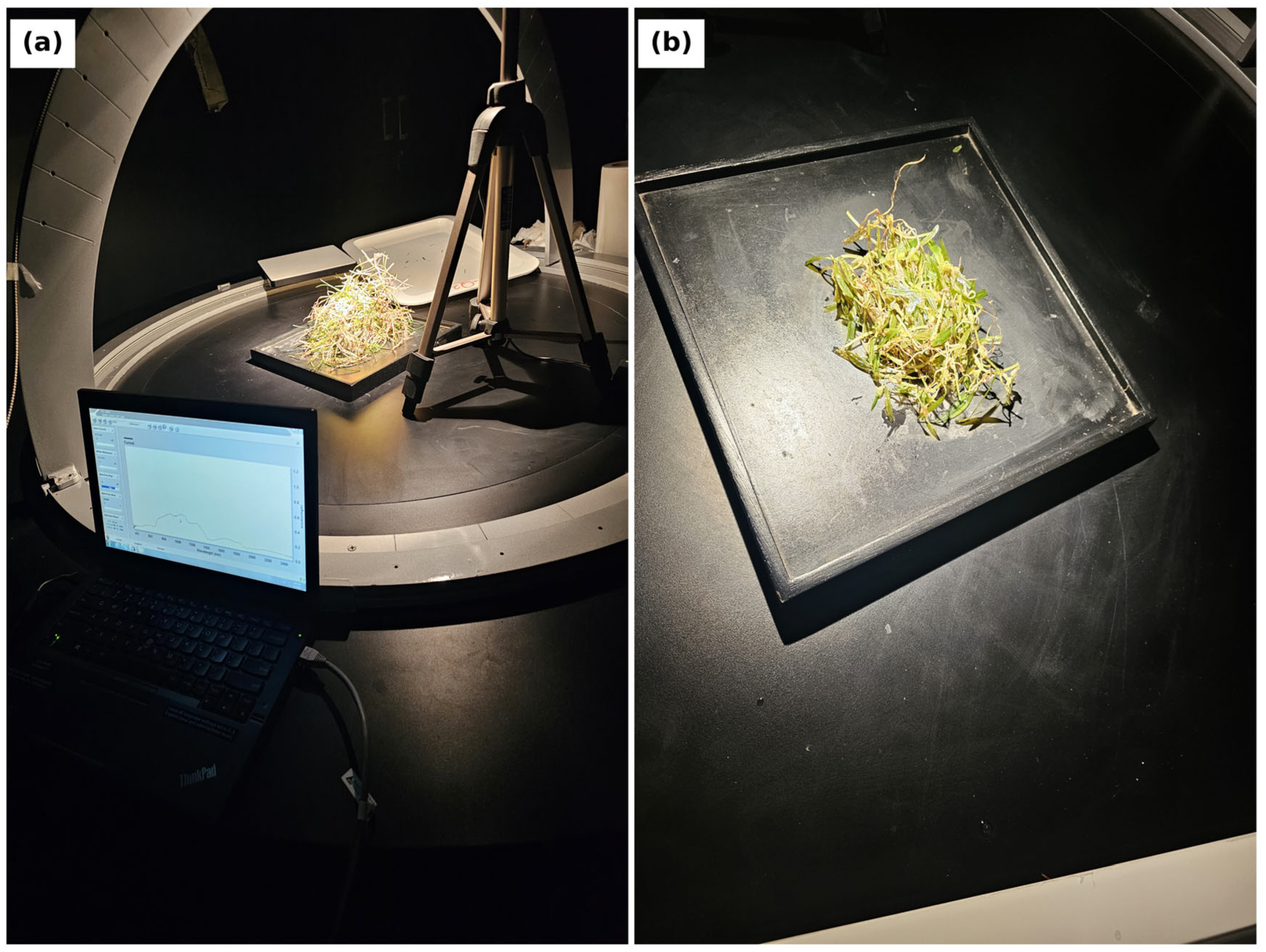
Figure 1.
Experimental workflow for acquiring seagrass spectral reflectance using the ASD FieldSpec® 4 Hi-Res spectroradiometer. (a) Full goniometer configuration in a darkened laboratory environment, with the collimated light source positioned on a precision tripod above the measurement platform and a laptop displaying real-time spectral output to verify data quality during acquisition. (b) Individual seagrass specimen placed on the dark reference panel within the goniometer platform, demonstrating the controlled, single-species measurement approach used to ensure reflectance purity and prevent cross-contamination between species.
Figure 1.
Experimental workflow for acquiring seagrass spectral reflectance using the ASD FieldSpec® 4 Hi-Res spectroradiometer. (a) Full goniometer configuration in a darkened laboratory environment, with the collimated light source positioned on a precision tripod above the measurement platform and a laptop displaying real-time spectral output to verify data quality during acquisition. (b) Individual seagrass specimen placed on the dark reference panel within the goniometer platform, demonstrating the controlled, single-species measurement approach used to ensure reflectance purity and prevent cross-contamination between species.
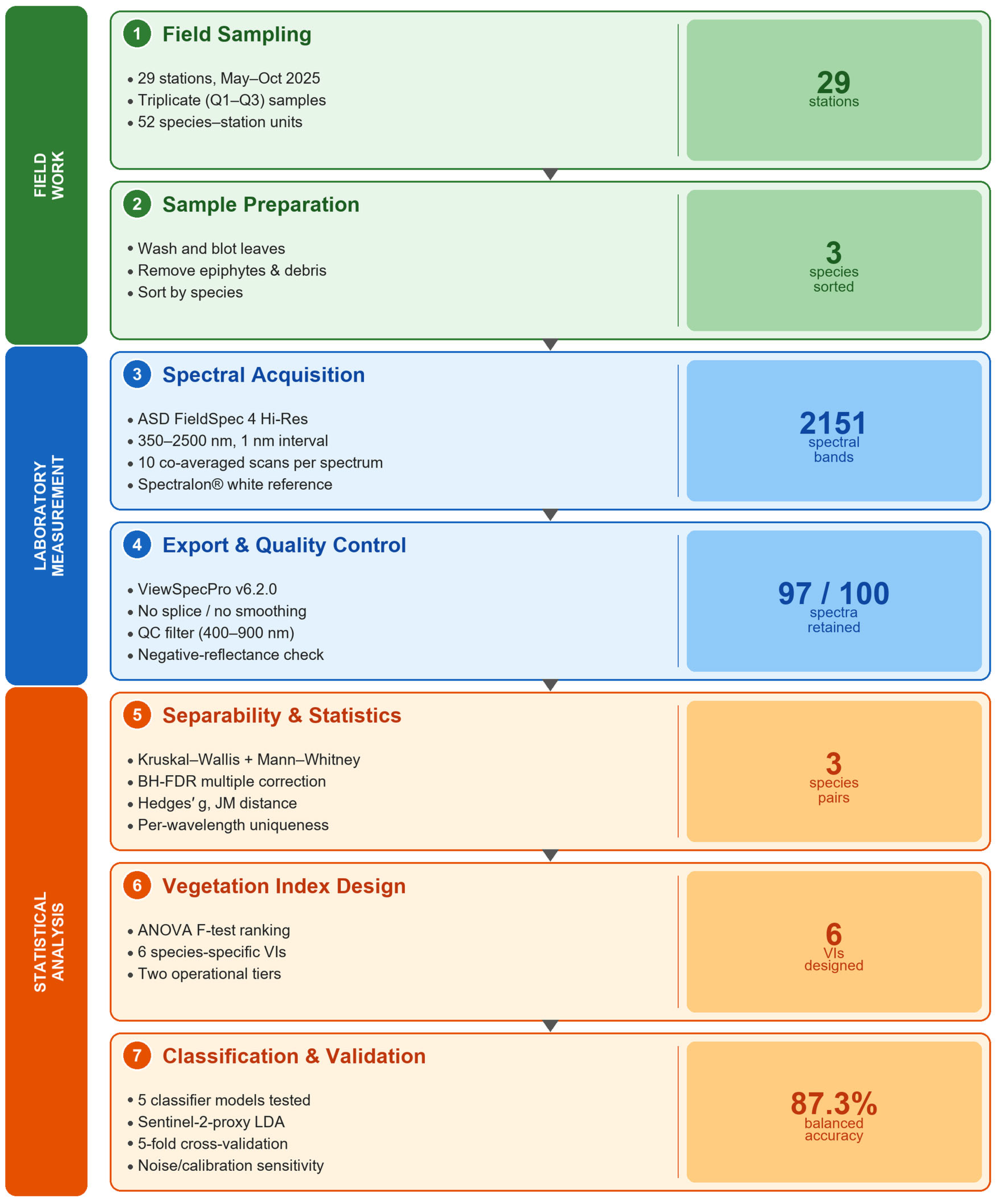
Figure 2.
Processing workflow for the spectral characterisation and classification of three Bahrain seagrass species, organised into three colour-coded phases: field work at 29 stations (May–Oct 2025), laboratory measurement with an ASD FieldSpec 4 Hi-Res spectroradiometer, and statistical analysis leading to six vegetation indices evaluated by five-fold cross-validation. Each step is annotated with its key output.
Figure 2.
Processing workflow for the spectral characterisation and classification of three Bahrain seagrass species, organised into three colour-coded phases: field work at 29 stations (May–Oct 2025), laboratory measurement with an ASD FieldSpec 4 Hi-Res spectroradiometer, and statistical analysis leading to six vegetation indices evaluated by five-fold cross-validation. Each step is annotated with its key output.
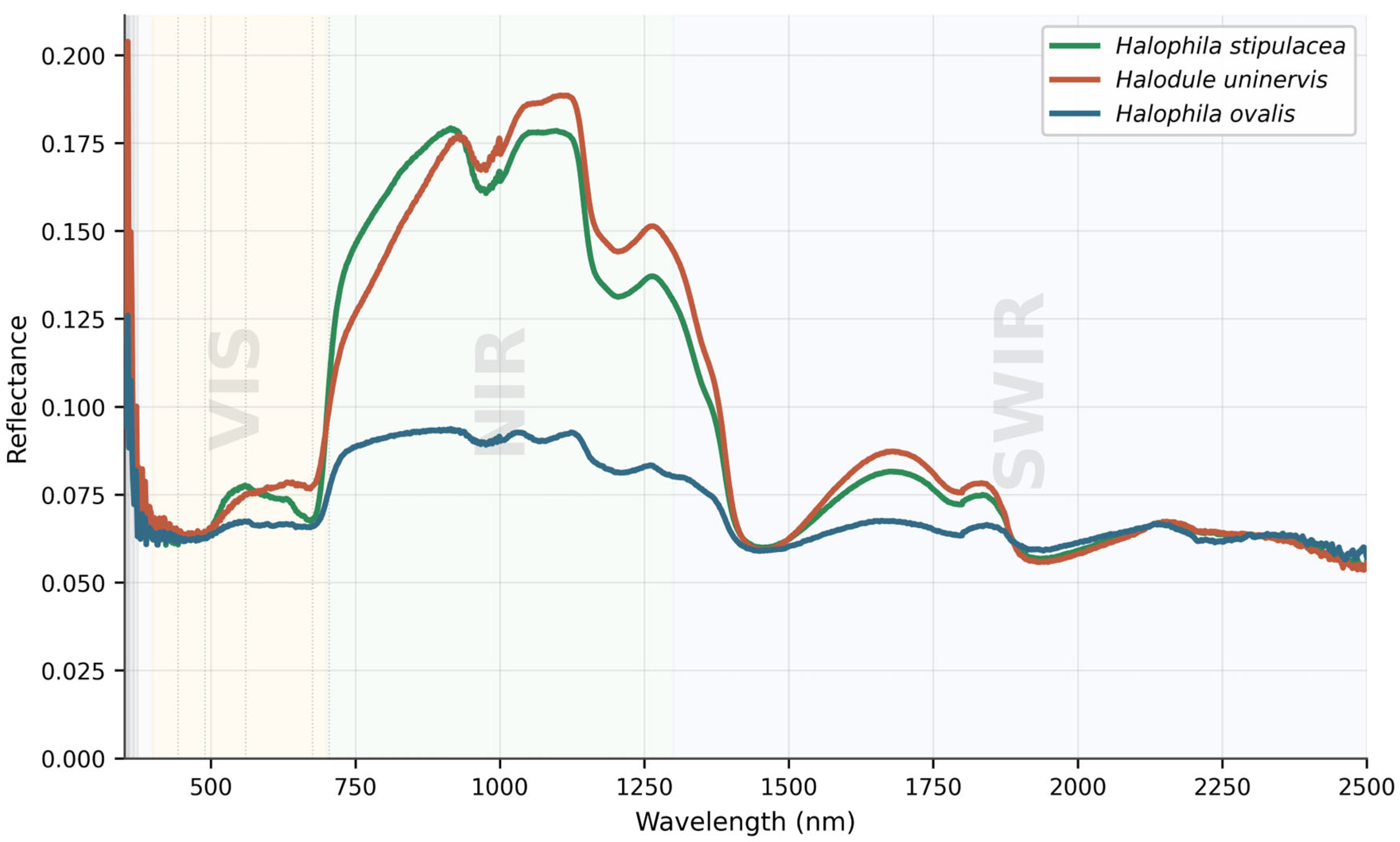
Figure 3.
Mean reflectance spectra (350–2500 nm) for the three Kingdom of Bahrain seagrass species. Shaded regions indicate major pigment absorption bands (blue, 400–500 nm; red, 650–700 nm) and the diagnostic red-edge region (690–740 nm).
Figure 3.
Mean reflectance spectra (350–2500 nm) for the three Kingdom of Bahrain seagrass species. Shaded regions indicate major pigment absorption bands (blue, 400–500 nm; red, 650–700 nm) and the diagnostic red-edge region (690–740 nm).
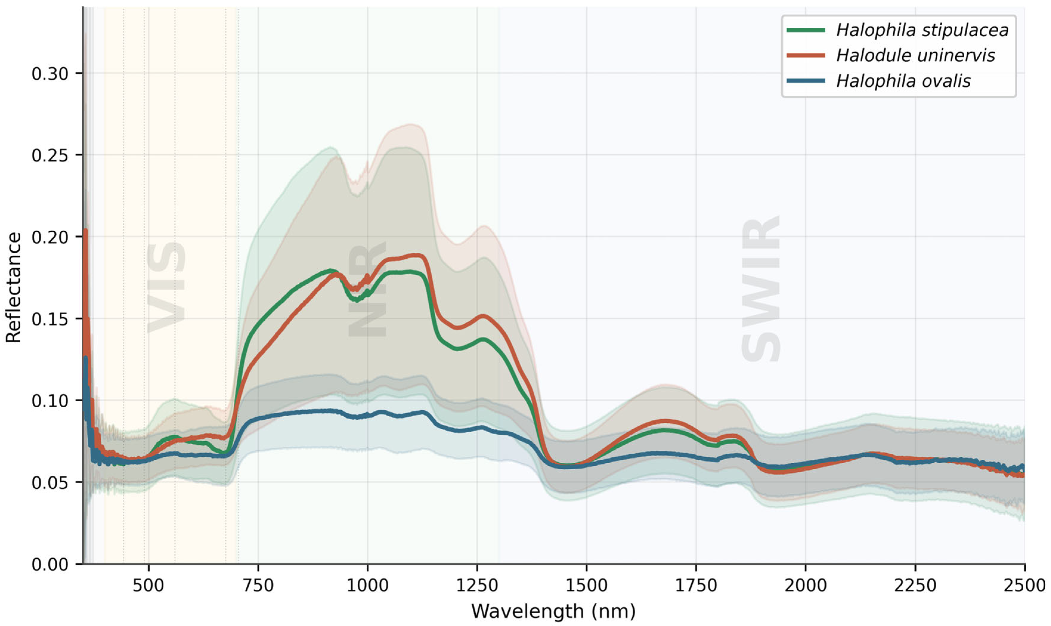
Figure 4.
Mean spectra with ±1 standard deviation (SD) envelopes for each species. Note the substantially wider near-infrared (NIR) variability in H. stipulacea and Hd. uninervis compared with H. ovalis. Colours: Halophila stipulacea (green), Halodule uninervis (red), Halophila ovalis (blue); shaded bands = ±1 SD envelopes.
Figure 4.
Mean spectra with ±1 standard deviation (SD) envelopes for each species. Note the substantially wider near-infrared (NIR) variability in H. stipulacea and Hd. uninervis compared with H. ovalis. Colours: Halophila stipulacea (green), Halodule uninervis (red), Halophila ovalis (blue); shaded bands = ±1 SD envelopes.
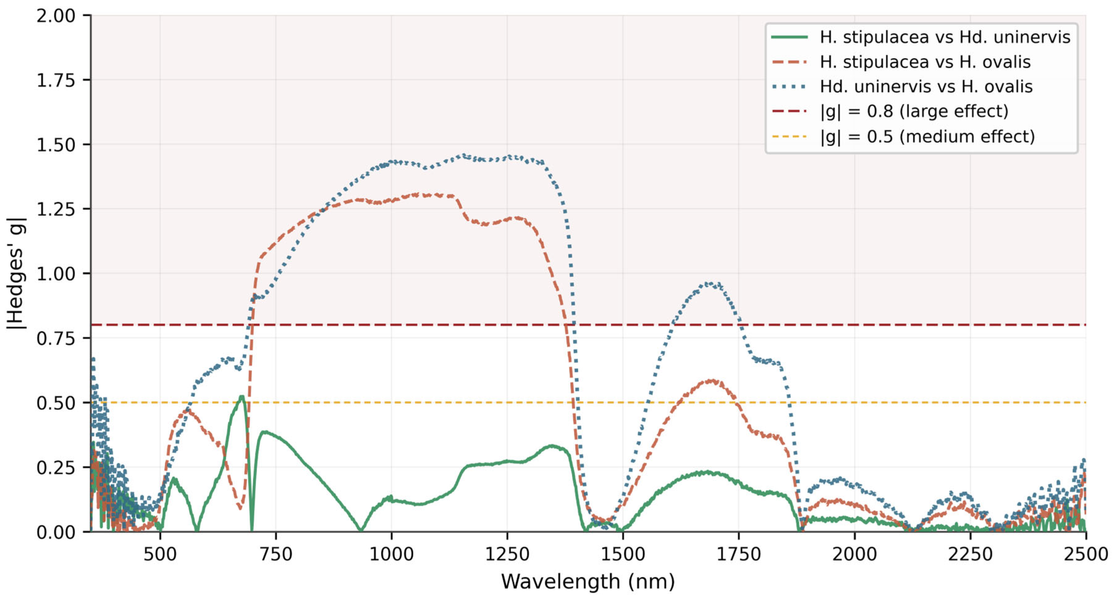
Figure 5.
Hedges’ g effect size profiles for all three pairwise species comparisons across 350–900 nm (visible to near-infrared—
shortwave-infrared (SWIR) discriminating windows extending to 1755 nm are reported in
Table 4 but fall outside this figure’s range). The horizontal dashed line indicates |g| = 0.8 (the large effect threshold). Shaded regions show wavelength windows meeting both Benjamini–
Hochberg (BH)-corrected significance (q < 0.05) and |g| ≥ 0.8.
Figure 5.
Hedges’ g effect size profiles for all three pairwise species comparisons across 350–900 nm (visible to near-infrared—
shortwave-infrared (SWIR) discriminating windows extending to 1755 nm are reported in
Table 4 but fall outside this figure’s range). The horizontal dashed line indicates |g| = 0.8 (the large effect threshold). Shaded regions show wavelength windows meeting both Benjamini–
Hochberg (BH)-corrected significance (q < 0.05) and |g| ≥ 0.8.
Figure 6.
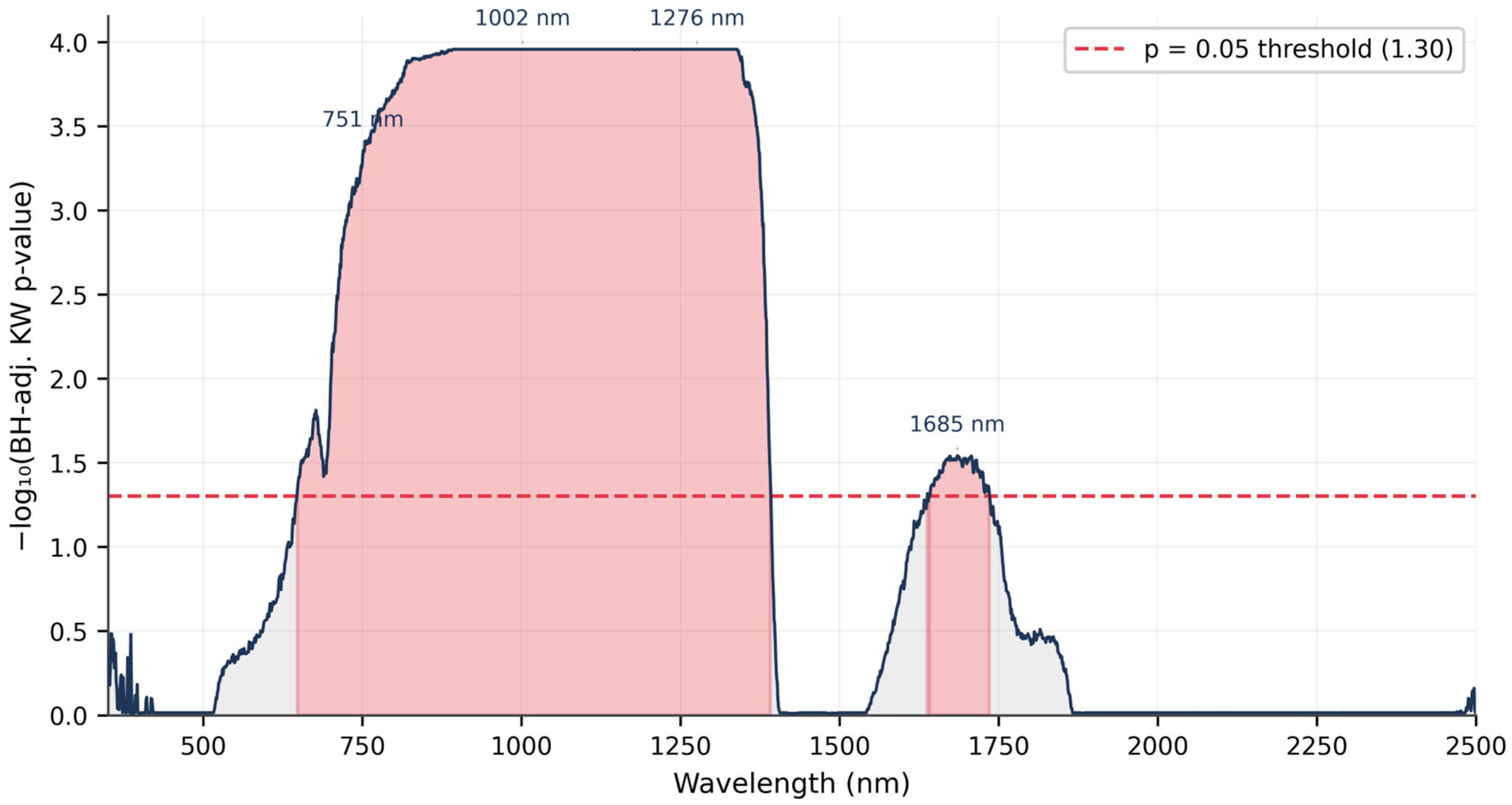
Kruskal–Wallis significance profiles: −log10(BH-adjusted p-value) at each wavelength for the three-way comparison. The horizontal dashed line corresponds to q = 0.05 (−log10 = 1.3). Red-shaded vertical bands mark the four retained discriminating windows (centred at 751, 1002, 1276 and 1685 nm) that satisfy both q < 0.05 and the large effect-size criterion.
Figure 6.
Kruskal–Wallis significance profiles: −log10(BH-adjusted p-value) at each wavelength for the three-way comparison. The horizontal dashed line corresponds to q = 0.05 (−log10 = 1.3). Red-shaded vertical bands mark the four retained discriminating windows (centred at 751, 1002, 1276 and 1685 nm) that satisfy both q < 0.05 and the large effect-size criterion.
Figure 7.
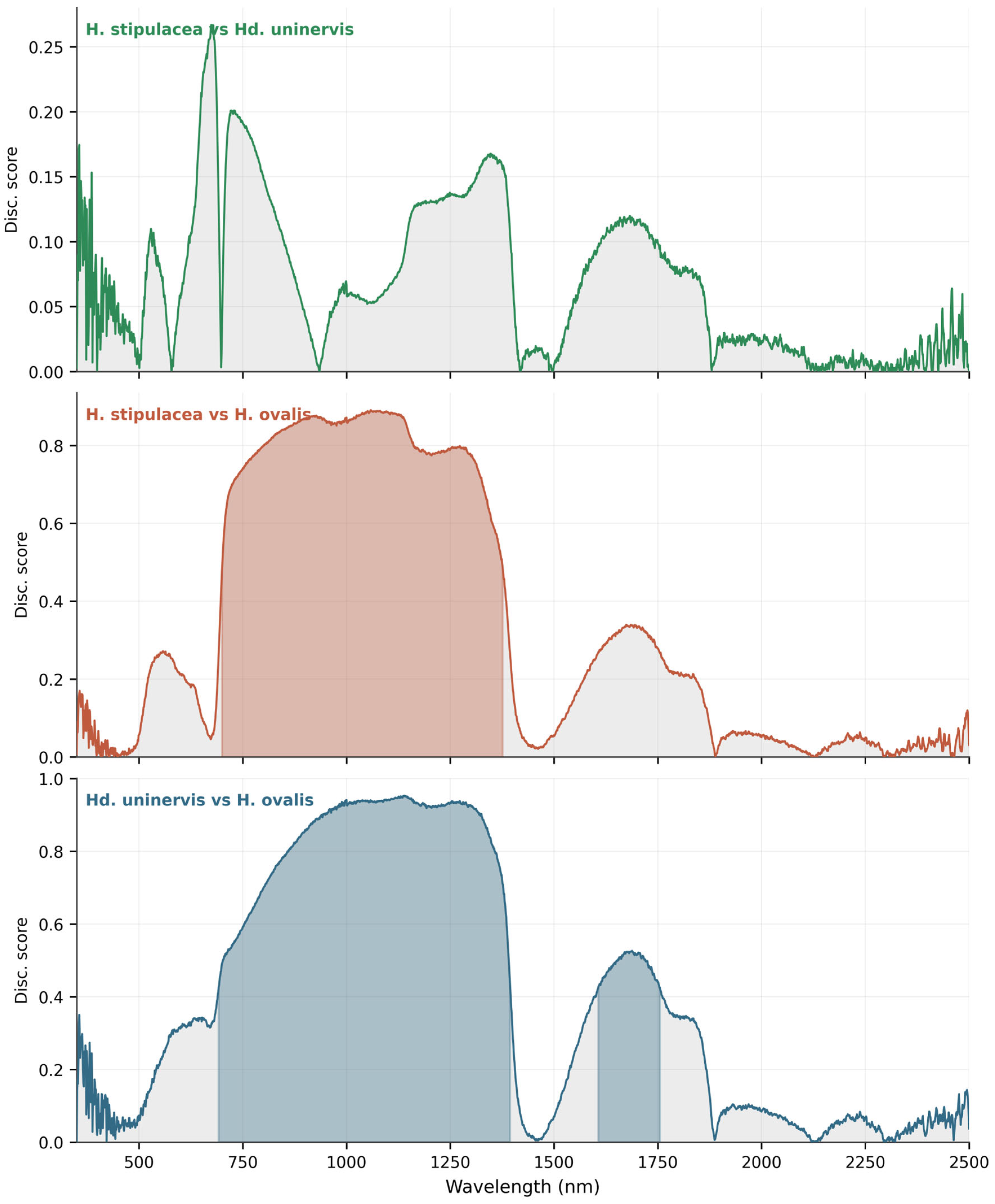
Per-wavelength separability (discrimination score) profiles for each pairwise species combination across 350–2500 nm. Peaks indicate wavelength regions with the highest inter-species contrast. Coloured shading marks the top discriminating wavelength bands for each pair; light grey shading marks secondary regions of elevated separability.
Figure 7.
Per-wavelength separability (discrimination score) profiles for each pairwise species combination across 350–2500 nm. Peaks indicate wavelength regions with the highest inter-species contrast. Coloured shading marks the top discriminating wavelength bands for each pair; light grey shading marks secondary regions of elevated separability.
Figure 8.
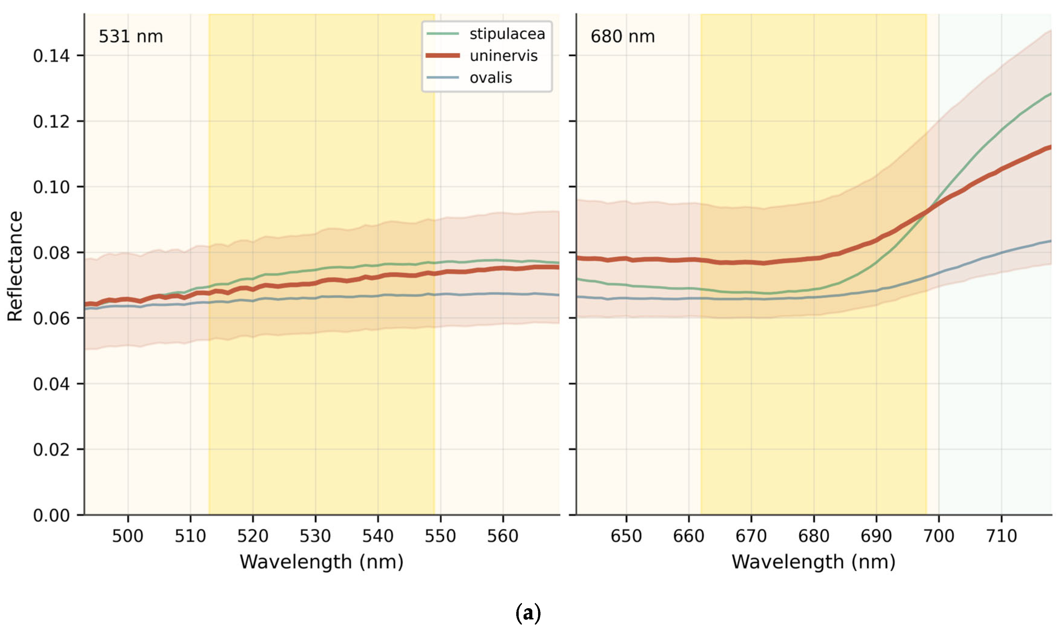
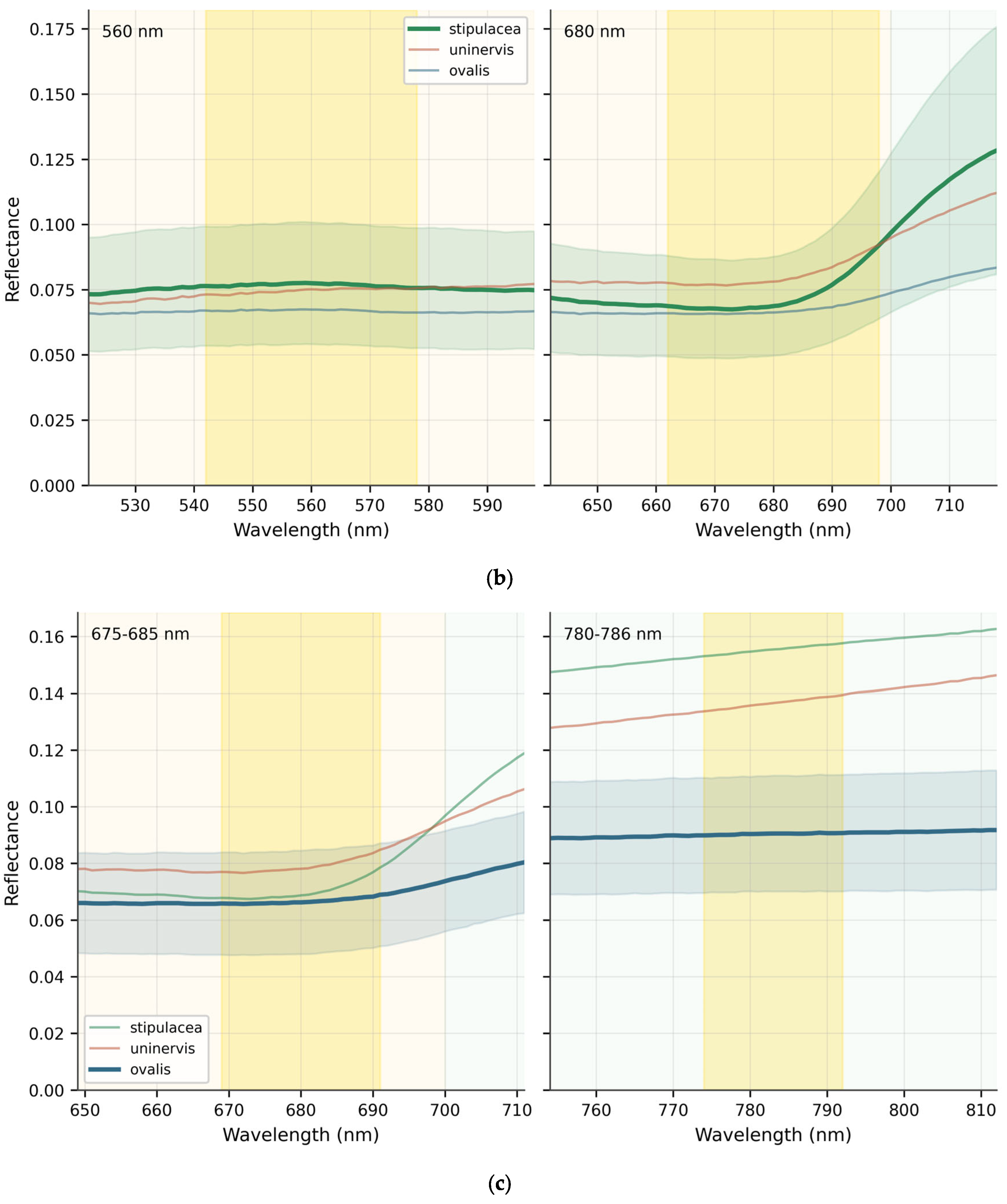
(a) Spectral uniqueness diagnostic windows for Hd. uninervis (HU_VIsub = ND(531, 680)). Yellow shading denotes the 513–549 nm (green) and 662–698 nm (red) reference bands used in the submerged-applicable index. The bold line with the ±1 SD envelope indicates the target species; thin lines show the other two species for comparison. (b) Spectral uniqueness diagnostic windows for H. stipulacea (HS_VI = ND(560, 680)). Yellow shading denotes the 542–578 nm (green) and 662–698 nm (red) reference bands used in the index. The bold line with the ±1 SD envelope indicates the target species; thin lines show the other two species for comparison. (c) Spectral uniqueness diagnostic windows for H. ovalis (HO_VIsub = DIFF(mean R675–685, mean R780–786)). Yellow shading denotes the 675–685 nm (red) and 780–786 nm (NIR) integration windows used in the submerged-applicable index. The bold line with the ±1 SD envelope indicates the target species; thin lines show the other two species for comparison.
Figure 8.
(a) Spectral uniqueness diagnostic windows for Hd. uninervis (HU_VIsub = ND(531, 680)). Yellow shading denotes the 513–549 nm (green) and 662–698 nm (red) reference bands used in the submerged-applicable index. The bold line with the ±1 SD envelope indicates the target species; thin lines show the other two species for comparison. (b) Spectral uniqueness diagnostic windows for H. stipulacea (HS_VI = ND(560, 680)). Yellow shading denotes the 542–578 nm (green) and 662–698 nm (red) reference bands used in the index. The bold line with the ±1 SD envelope indicates the target species; thin lines show the other two species for comparison. (c) Spectral uniqueness diagnostic windows for H. ovalis (HO_VIsub = DIFF(mean R675–685, mean R780–786)). Yellow shading denotes the 675–685 nm (red) and 780–786 nm (NIR) integration windows used in the submerged-applicable index. The bold line with the ±1 SD envelope indicates the target species; thin lines show the other two species for comparison.


Figure 9.
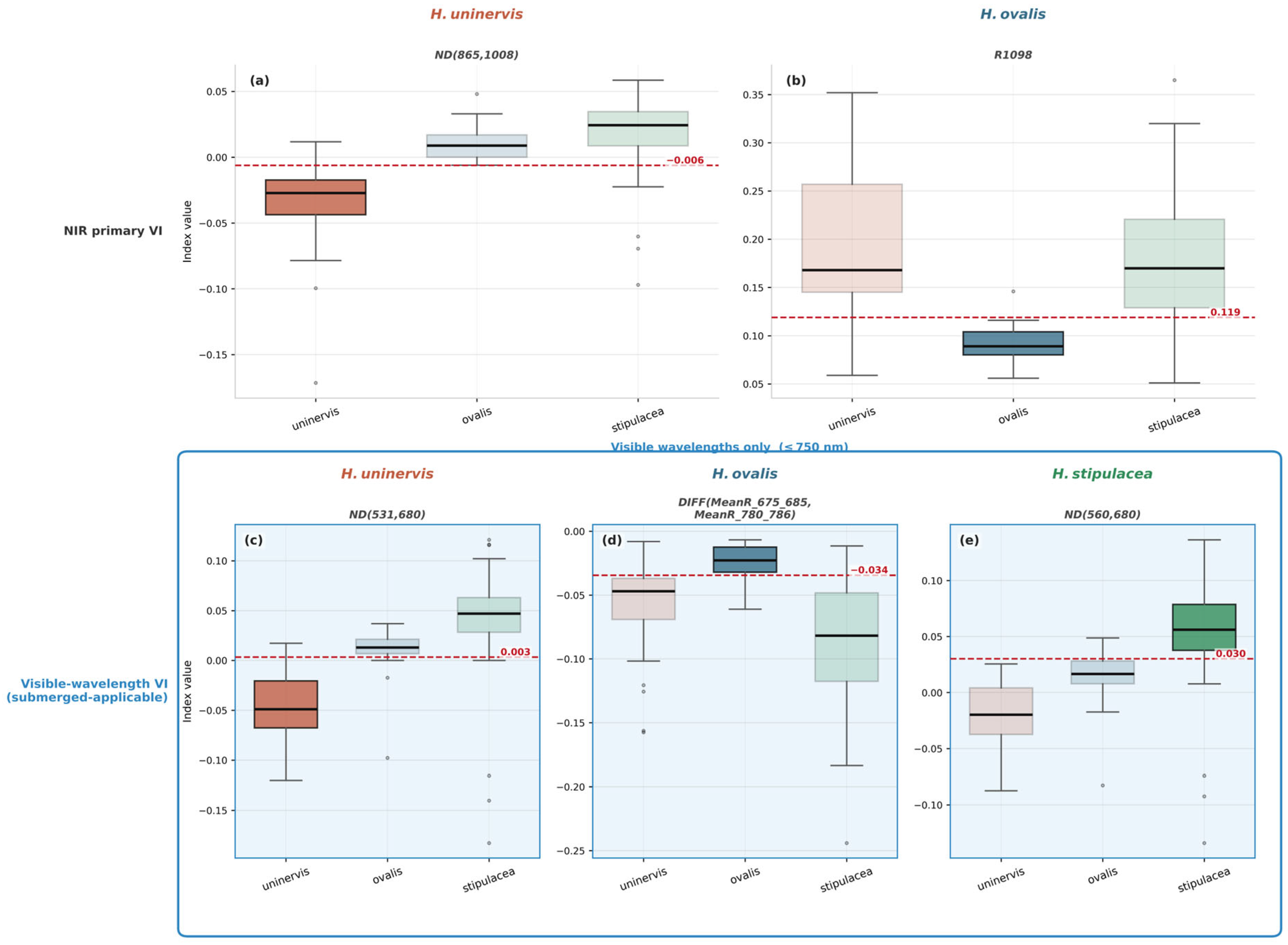
Distribution of species-specific vegetation index values across all three species, with optimal classification thresholds (dashed red line) overlaid. Top row—NIR-based primary VIs: (a) HU_vegetation index (VI) [ND(865, 1008)] for Hd. Uninervis, and (b) HO_VI [R1098] for H. ovalis. Bottom row (shaded, visible wavelengths ≤ 750 nm)—submerged-applicable VIs: (c) HU_VIsub [ND(531, 680)] for Hd. uninervis; (d) HO_VIsub [mean(R675–685) − mean(R780–786)] for H. ovalis; and (e) HS_VI [ND(560, 680)] for H. stipulacea, whose best-overall VI already operates in the visible range and is therefore both the primary and submerged-applicable index. Box plots show a median, an interquartile range, and outliers; the highlighted box corresponds to the target species for each index.
Figure 9.
Distribution of species-specific vegetation index values across all three species, with optimal classification thresholds (dashed red line) overlaid. Top row—NIR-based primary VIs: (a) HU_vegetation index (VI) [ND(865, 1008)] for Hd. Uninervis, and (b) HO_VI [R1098] for H. ovalis. Bottom row (shaded, visible wavelengths ≤ 750 nm)—submerged-applicable VIs: (c) HU_VIsub [ND(531, 680)] for Hd. uninervis; (d) HO_VIsub [mean(R675–685) − mean(R780–786)] for H. ovalis; and (e) HS_VI [ND(560, 680)] for H. stipulacea, whose best-overall VI already operates in the visible range and is therefore both the primary and submerged-applicable index. Box plots show a median, an interquartile range, and outliers; the highlighted box corresponds to the target species for each index.
Figure 10.
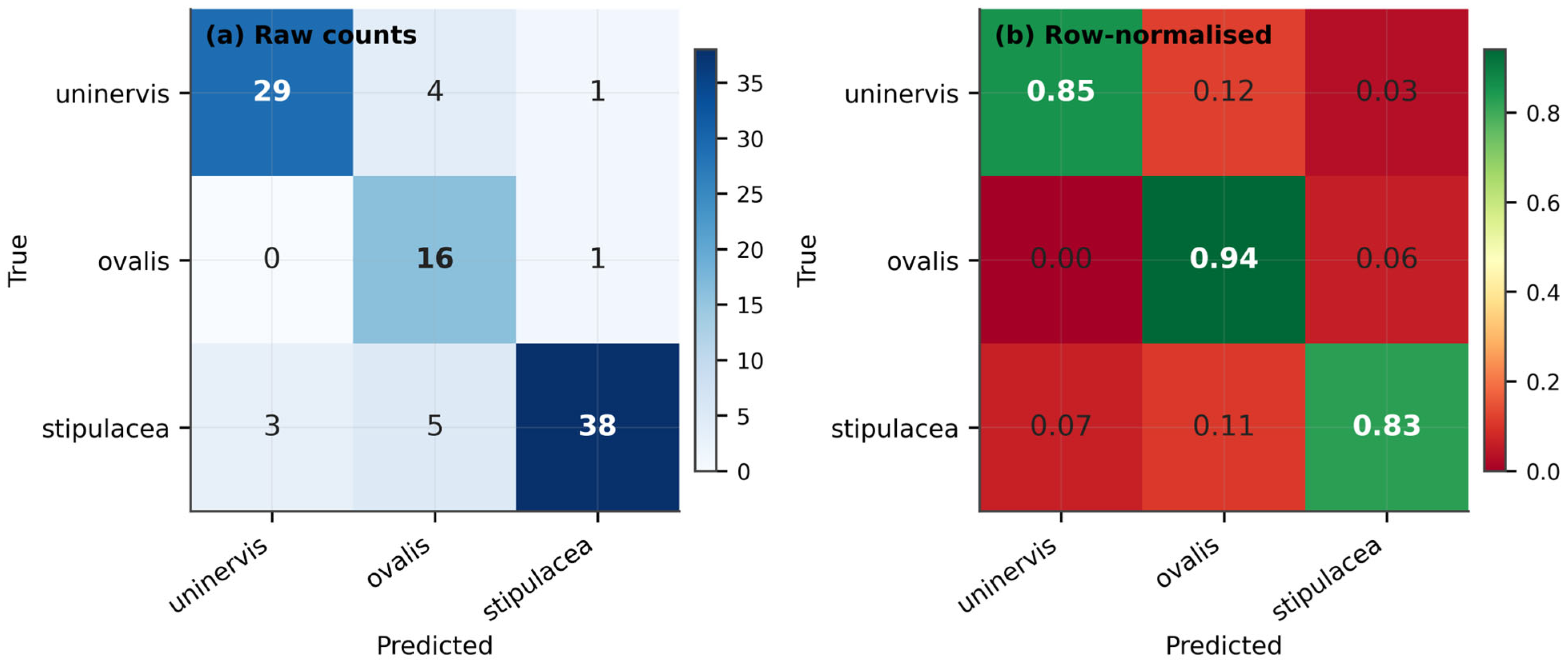
Confusion matrices for the Sentinel-2-proxy LDA classifier (repeated stratified k-fold cross-validation—k = 5 folds, 5 repeats): raw counts (a) and row-normalised proportions (b). Diagonal cells show correctly classified spectra.
Figure 10.
Confusion matrices for the Sentinel-2-proxy LDA classifier (repeated stratified k-fold cross-validation—k = 5 folds, 5 repeats): raw counts (a) and row-normalised proportions (b). Diagonal cells show correctly classified spectra.
Figure 11.
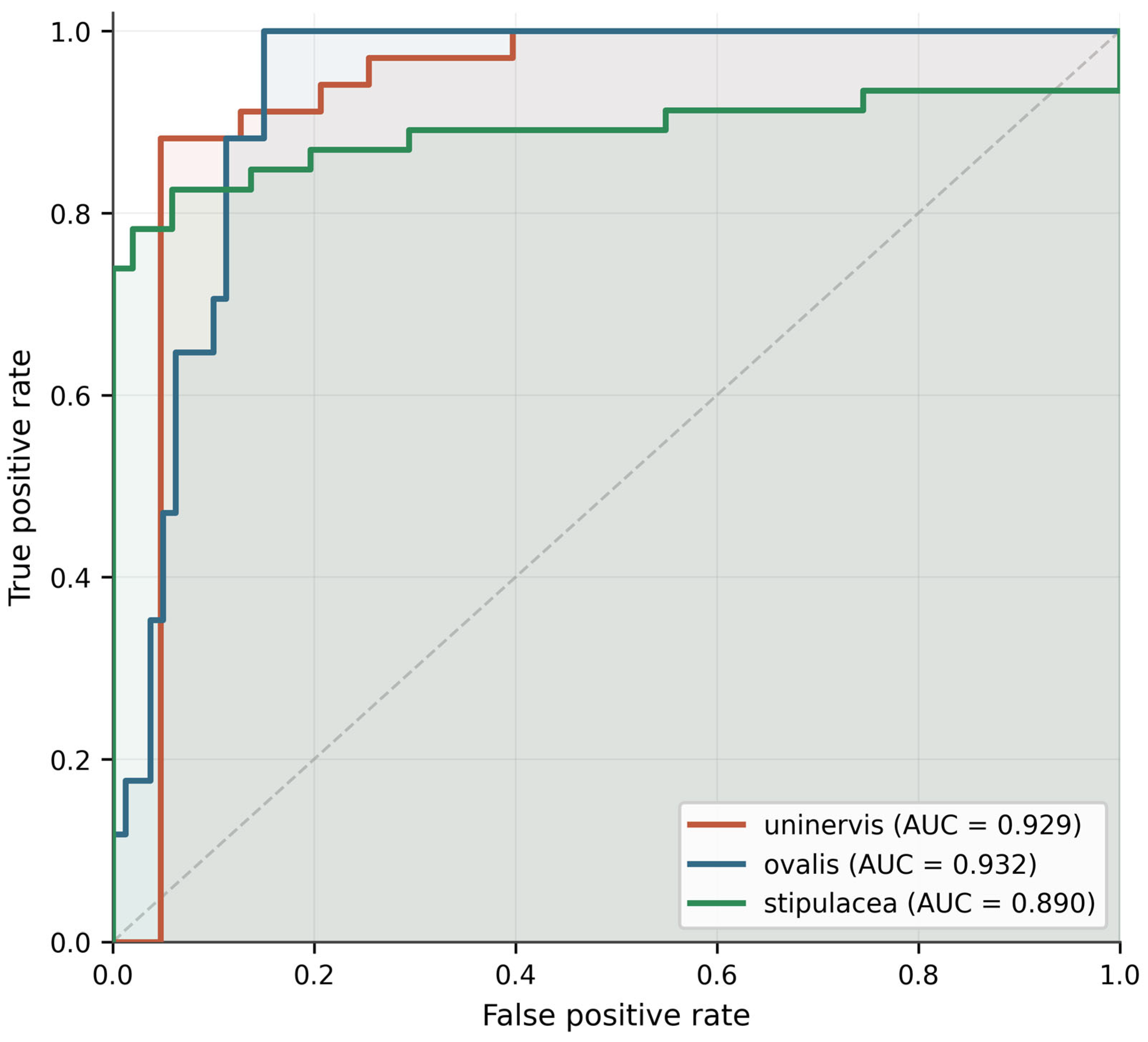
One-versus-rest receiver operating characteristic (ROC) curves for each species class from the Sentinel-2-proxy LDA. AUC values are inset. The diagonal dashed line represents the random classifier baseline.
Figure 11.
One-versus-rest receiver operating characteristic (ROC) curves for each species class from the Sentinel-2-proxy LDA. AUC values are inset. The diagonal dashed line represents the random classifier baseline.
Figure 12.
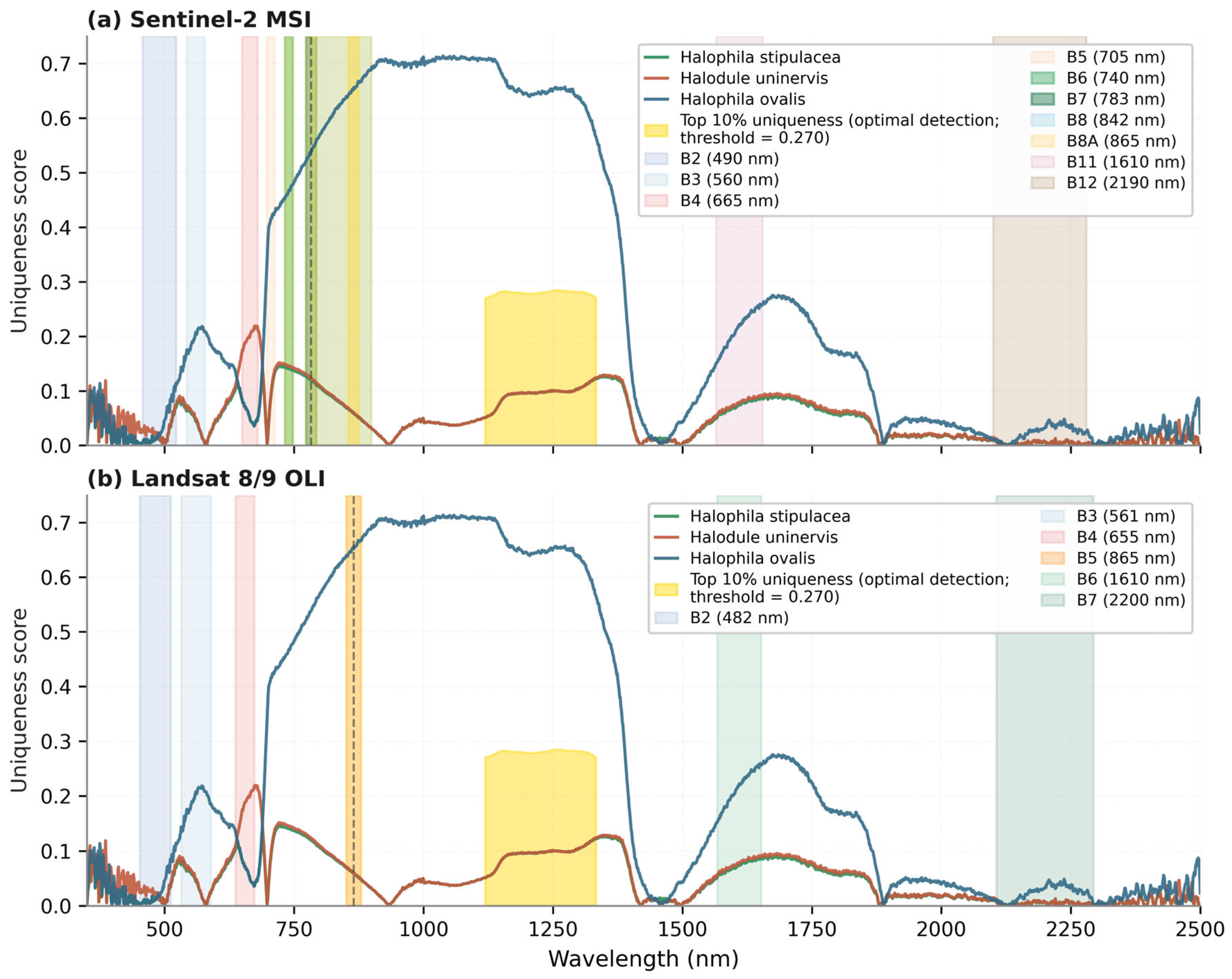
Per-species spectral uniqueness profiles overlaid with sensor band extents for (a) Sentinel-2 MultiSpectral Instrument (MSI) and (b) Landsat 8/9 Operational Land Imager (OLI). Uniqueness score (dimensionless, ≥0; observed maximum ≈ 0.71 in this dataset) quantifies each species’ spectral distinctiveness relative to the other two co-occurring taxa at each wavelength; higher values indicate greater potential for single-wavelength identification. The yellow-filled area denotes the wavelength region where the cross-species mean uniqueness exceeds the 90th-percentile threshold (=0.270), representing the optimal detection window, which is centred in the 950–1350 nm NIR plateau in this case, driven primarily by the distinctive NIR response of H. ovalis. Coloured vertical spans show sensor band extents; bands whose mean uniqueness score reaches ≥80% of the threshold are displayed at higher opacity. The dashed vertical line indicates the centre wavelength of the single highest-ranking band for each sensor. Note: NIR features (≳750 nm) are subject to strong water-column attenuation and primarily applicable to above-water, very-shallow (≲1 m), or low-tide measurements.
Figure 12.
Per-species spectral uniqueness profiles overlaid with sensor band extents for (a) Sentinel-2 MultiSpectral Instrument (MSI) and (b) Landsat 8/9 Operational Land Imager (OLI). Uniqueness score (dimensionless, ≥0; observed maximum ≈ 0.71 in this dataset) quantifies each species’ spectral distinctiveness relative to the other two co-occurring taxa at each wavelength; higher values indicate greater potential for single-wavelength identification. The yellow-filled area denotes the wavelength region where the cross-species mean uniqueness exceeds the 90th-percentile threshold (=0.270), representing the optimal detection window, which is centred in the 950–1350 nm NIR plateau in this case, driven primarily by the distinctive NIR response of H. ovalis. Coloured vertical spans show sensor band extents; bands whose mean uniqueness score reaches ≥80% of the threshold are displayed at higher opacity. The dashed vertical line indicates the centre wavelength of the single highest-ranking band for each sensor. Note: NIR features (≳750 nm) are subject to strong water-column attenuation and primarily applicable to above-water, very-shallow (≲1 m), or low-tide measurements.

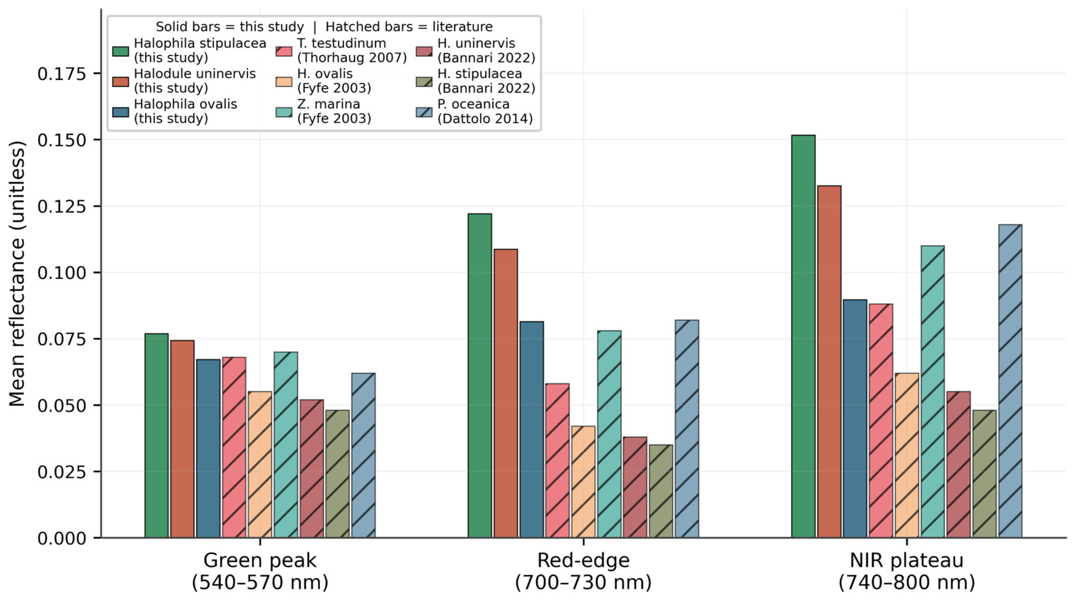
Figure 13.
Quantitative comparison of mean reflectance values from this study against published values for seagrass species in equivalent spectral bands across three spectral regions: green peak (540–570 nm), red-edge (700–730 nm), and NIR plateau (740–800 nm). Solid bars = this study (three Kingdom of Bahrain seagrass species); hatched bars = values from the literature. Sources: Thorhaug et al. [
50] (
T. testudinum); Fyfe [
5] (
H. ovalis,
Z. marina); Bannari et al. [
20] (
Hd. uninervis,
H. stipulacea); Dattolo et al. [
51] (
P. oceanica).
Figure 13.
Quantitative comparison of mean reflectance values from this study against published values for seagrass species in equivalent spectral bands across three spectral regions: green peak (540–570 nm), red-edge (700–730 nm), and NIR plateau (740–800 nm). Solid bars = this study (three Kingdom of Bahrain seagrass species); hatched bars = values from the literature. Sources: Thorhaug et al. [
50] (
T. testudinum); Fyfe [
5] (
H. ovalis,
Z. marina); Bannari et al. [
20] (
Hd. uninervis,
H. stipulacea); Dattolo et al. [
51] (
P. oceanica).
Table 1.
Dataset overview: sample and station counts, quality-control retention, and depth ranges by species.
Table 1.
Dataset overview: sample and station counts, quality-control retention, and depth ranges by species.
| Species | Code | n Spectra (Total) | n Retained | n Excluded | % Retained | n Stations |
|---|
| Halophila stipulacea | A | 47 | 46 | 1 | 98% | 25 |
| Halodule uninervis | B | 36 | 34 | 2 | 94% | 19 |
| Halophila ovalis | C | 17 | 17 | 0 | 100% | 8 |
Table 2.
Mean reflectance (±SD) at key diagnostic wavelengths according to species.
Table 2.
Mean reflectance (±SD) at key diagnostic wavelengths according to species.
| Wavelength (nm) | Region | H. stipulacea (Mean ± SD) | Hd. uninervis (Mean ± SD) | H. ovalis (Mean ± SD) |
|---|
| 443 | Violet | 0.0607 ± 0.0179 | 0.0616 ± 0.0135 | 0.0614 ± 0.0135 |
| 490 | Blue | 0.0636 ± 0.0190 | 0.0644 ± 0.0141 | 0.0629 ± 0.0144 |
| 531 | Green | 0.0750 ± 0.0226 | 0.0712 ± 0.0155 | 0.0665 ± 0.0140 |
| 560 | Green | 0.0775 ± 0.0234 | 0.0751 ± 0.0169 | 0.0674 ± 0.0141 |
| 620 | Red | 0.0738 ± 0.0219 | 0.0778 ± 0.0177 | 0.0666 ± 0.0166 |
| 665 | Red | 0.0680 ± 0.0191 | 0.0768 ± 0.0169 | 0.0657 ± 0.0180 |
| 705 | Red edge | 0.1078 ± 0.0361 | 0.1004 ± 0.0284 | 0.0768 ± 0.0178 |
| 740 | Red edge | 0.1425 ± 0.0560 | 0.1232 ± 0.0426 | 0.0877 ± 0.0195 |
| 783 | NIR | 0.1554 ± 0.0628 | 0.1366 ± 0.0494 | 0.0905 ± 0.0205 |
| 800 | NIR | 0.1596 ± 0.0650 | 0.1421 ± 0.0522 | 0.0911 ± 0.0207 |
| 865 | NIR | 0.1728 ± 0.0722 | 0.1614 ± 0.0630 | 0.0929 ± 0.0220 |
Table 3.
Pairwise spectral separability metrics across 350–900 nm for all three species pairs.
Table 3.
Pairwise spectral separability metrics across 350–900 nm for all three species pairs.
| Species Pair | n_A | n_B | Euclidean Dist. | SAM (°) | MAD | RMSE | Bhattacharyya (PCA) | JM Dist. (PCA) |
|---|
| H. stipulacea vs. Hd. uninervis | 46 | 34 | 0.3481 | 3.9972 | 0.0052 | 0.0075 | 0.6875 | 0.9944 |
| H. stipulacea vs. H. ovalis | 46 | 17 | 1.7728 | 14.8641 | 0.0238 | 0.0383 | 1.6199 | 1.6041 |
| Hd. uninervis vs. H. ovalis | 34 | 17 | 1.8635 | 15.1583 | 0.0258 | 0.0403 | 1.7889 | 1.6657 |
Table 4.
Discriminating spectral windows: start and end wavelengths, mean Hedges’ |g|, and minimum BH-corrected q-value for each species pair. † Windows listed for H. stipulacea vs. Hd. uninervis are candidate windows only; neither one meets the combined criteria for BH significance (q < 0.05) and large effect size (|g| ≥ 0.8) required for a confirmed discriminating window.
Table 4.
Discriminating spectral windows: start and end wavelengths, mean Hedges’ |g|, and minimum BH-corrected q-value for each species pair. † Windows listed for H. stipulacea vs. Hd. uninervis are candidate windows only; neither one meets the combined criteria for BH significance (q < 0.05) and large effect size (|g| ≥ 0.8) required for a confirmed discriminating window.
| Species Pair | Window (nm) | Width (nm) | Mean |g| | Min q | Higher Reflectance |
|---|
| H. stipulacea vs. Hd. uninervis | 648–688 | 41 | 0.473 | 0.688 | Hd. uninervis |
| H. stipulacea vs. Hd. uninervis | 721–732 | 12 | 0.384 | 0.981 | H. stipulacea |
| H. stipulacea vs. H. ovalis | 700–1376 | 677 | 1.206 | 0.000285 | H. stipulacea |
| Hd. uninervis vs. H. ovalis | 692–1394 | 703 | 1.313 | 4.6 × 10⁻⁵ | Hd. uninervis |
| Hd. uninervis vs. H. ovalis | 1607–1755 | 149 | 0.903 | 0.00602 | Hd. uninervis |
Table 5.
Top discriminating wavelengths per species, ranked by uniqueness score U(λ, s) (
Section 2.4).
Table 5.
Top discriminating wavelengths per species, ranked by uniqueness score U(λ, s) (
Section 2.4).
| Species | Wavelength (nm) | Region | Uniqueness Score |
|---|
| Hd. uninervis | 674 | Red | 0.2191 |
| Hd. uninervis | 677 | Red | 0.2189 |
| Hd. uninervis | 675 | Red | 0.2187 |
| Hd. uninervis | 679 | Red | 0.2186 |
| Hd. uninervis | 673 | Red | 0.2168 |
| Hd. uninervis | 678 | Red | 0.2159 |
| Hd. uninervis | 676 | Red | 0.2147 |
| Hd. uninervis | 680 | Red | 0.2123 |
| H. ovalis | 1038 | SWIR | 0.7141 |
| H. ovalis | 1059 | SWIR | 0.7138 |
| H. ovalis | 1058 | SWIR | 0.7133 |
| H. ovalis | 1051 | SWIR | 0.7132 |
| H. ovalis | 1073 | SWIR | 0.7131 |
| H. ovalis | 1074 | SWIR | 0.7129 |
| H. ovalis | 1050 | SWIR | 0.7129 |
| H. ovalis | 1000 | SWIR | 0.7124 |
| H. stipulacea | 721 | Red edge | 0.146 |
| H. stipulacea | 722 | Red edge | 0.146 |
| H. stipulacea | 723 | Red edge | 0.1458 |
| H. stipulacea | 725 | Red edge | 0.1452 |
| H. stipulacea | 724 | Red edge | 0.1452 |
| H. stipulacea | 729 | Red edge | 0.1452 |
| H. stipulacea | 731 | Red edge | 0.1449 |
| H. stipulacea | 728 | Red edge | 0.1447 |
Table 6.
Species-specific vegetation indices: formulation, optimal threshold, balanced accuracy, and area under the curve (AUC).
Table 6.
Species-specific vegetation indices: formulation, optimal threshold, balanced accuracy, and area under the curve (AUC).
| Target Species | Index Formula | Submerged Applicable | Threshold | Bal. Accuracy | AUC | Dir. Consistency |
|---|
| Hd. uninervis | HU_VI = (R_865 − R_1008)/(R_865 + R_1008) | No | −0.0062 | 0.9241 | 0.9388 | 1.0 |
| Hd. uninervis | HU_VI = (R_531 − R_680)/(R_531 + R_680) | Yes | 0.0034 | 0.9071 | 0.9232 | 1.0 |
| H. ovalis | HO_VI = R_1098 | No | 0.119 | 0.8768 | 0.8643 | 1.0 |
| H. ovalis | HO_VI = mean(R_675:685) − mean(R_780:786) | Yes | −0.0344 | 0.818 | 0.8529 | 1.0 |
| H. stipulacea | HS_VI = (R_560 − R_680)/(R_560 + R_680) | Yes | 0.0302 | 0.8836 | 0.902 | 1.0 |
Table 7.
Repeated stratified k-fold cross-validated performance (k = 5, 5 repeats) for all five classifier models: two decision-tree baselines and three linear discriminant analysis (LDA) configurations. Metrics: overall accuracy, balanced accuracy, macro F1, and macro one-versus-rest AUC.
Table 7.
Repeated stratified k-fold cross-validated performance (k = 5, 5 repeats) for all five classifier models: two decision-tree baselines and three linear discriminant analysis (LDA) configurations. Metrics: overall accuracy, balanced accuracy, macro F1, and macro one-versus-rest AUC.
| Rank | Model | Feature Family | Estimator | Accuracy | Bal. Accuracy | F1-Macro | AUC (Macro OvR) |
|---|
| 1 | Sentinel-2 proxy 4-index LDA | sentinel2_proxy_lda | LDA | 0.8557 | 0.8734 | 0.8415 | 0.917 |
| 2 | Best single exploratory feature | single_feature | DecisionTree | 0.7835 | 0.7954 | 0.7647 | 0.8731 |
| 3 | Adapted 3-index LDA | adapted_standard_lda | LDA | 0.7835 | 0.7805 | 0.7581 | 0.8877 |
| 4 | Custom pairwise feature tree | pairwise_tree | DecisionTree | 0.732 | 0.7246 | 0.702 | 0.8265 |
| 5 | Landsat proxy 3-index LDA | landsat_proxy_lda | LDA | 0.732 | 0.6726 | 0.6726 | 0.8544 |
Table 8.
Alignment of Sentinel-2 MSI and Landsat 8/9 OLI band centres with the five diagnostic wavelengths identified in this study. Offsets > 10 nm are flagged †.
Table 8.
Alignment of Sentinel-2 MSI and Landsat 8/9 OLI band centres with the five diagnostic wavelengths identified in this study. Offsets > 10 nm are flagged †.
| Diagnostic Wavelength (nm) | Sensor | Nearest Band | Band Centre (nm) | Bandwidth (nm) | Offset from Target (nm) |
|---|
| 560 | Sentinel-2 | B3 (Green) | 560 | 35 | 0 |
| 560 | Landsat 8/9 | B3 (Green) | 561 | 57 | 1 |
| 665 | Sentinel-2 | B4 (Red) | 665 | 30 | 0 |
| 665 | Landsat 8/9 | B4 (Red) | 655 | 37 | 10 |
| 705 | Sentinel-2 | B5 (Red-edge) | 705 | 15 | 0 |
| 705 | Landsat 8/9 | B4 (Red) | 655 | 37 | 50 † |
| 740 | Sentinel-2 | B6 (Red-edge) | 740 | 15 | 0 |
| 740 | Landsat 8/9 | B4 (Red) | 655 | 37 | 85 † |
| 783 | Sentinel-2 | B7 (NIR) | 783 | 20 | 0 |
| 783 | Landsat 8/9 | B5 (NIR) | 865 | 28 | 82 † |
Table 9.
Sensitivity analysis: The balanced accuracy of the Sentinel-2-proxy LDA under increasing levels of Gaussian noise (σ), a reflectance quantisation step, and wavelength misregistration (±nm). Changes are reported as percentage-point differences from the unperturbed baseline (82.4%) †.
Table 9.
Sensitivity analysis: The balanced accuracy of the Sentinel-2-proxy LDA under increasing levels of Gaussian noise (σ), a reflectance quantisation step, and wavelength misregistration (±nm). Changes are reported as percentage-point differences from the unperturbed baseline (82.4%) †.
| Perturbation Type | Level | Bal. Accuracy | Δ from Baseline (pp) |
|---|
| Baseline (no perturbation) | — | 0.8244 | 0.0 |
| Gaussian noise (σ) | +0.001 | 0.8171 | −0.72 |
| Gaussian noise (σ) | +0.002 | 0.7489 | −7.54 |
| Gaussian noise (σ) | +0.005 | 0.6436 | −18.07 |
| Reflectance quantisation (step) | +0.001 | 0.8244 | 0.0 |
| Reflectance quantisation (step) | +0.002 | 0.8073 | −1.71 |
| Reflectance quantisation (step) | +0.005 | 0.7417 | −8.27 |
| Reflectance quantisation (step) | +0.01 | 0.6066 | −21.78 |
| Wavelength shift (nm) | −3 | 0.6944 | −13.0 |
| Wavelength shift (nm) | −2 | 0.7694 | −5.5 |
| Wavelength shift (nm) | −1 | 0.8274 | 0.3 |
| Wavelength shift (nm) | +1 | 0.8022 | −2.22 |
| Wavelength shift (nm) | +2 | 0.7187 | −10.57 |
| Wavelength shift (nm) | +3 | 0.6671 | −15.73 |
Table 10.
Top-ranking Kruskal–Wallis wavelengths (three-way H-test, BH-corrected) with H-statistic, BH q-value, and spectral region. See
Figure 6 for the full significance profile across the measured spectrum.
Table 10.
Top-ranking Kruskal–Wallis wavelengths (three-way H-test, BH-corrected) with H-statistic, BH q-value, and spectral region. See
Figure 6 for the full significance profile across the measured spectrum.
| Wavelength (nm) | Region | KW H Statistic | BH-adj. q Value | −log10(q) |
|---|
| 1339 | SWIR | 21.53 | 0.000111 | 3.96 |
| 1338 | SWIR | 21.61 | 0.000111 | 3.96 |
| 1337 | SWIR | 21.45 | 0.000111 | 3.96 |
| 1336 | SWIR | 21.59 | 0.000111 | 3.96 |
| 1335 | SWIR | 21.73 | 0.000111 | 3.96 |
| 1334 | SWIR | 21.85 | 0.000111 | 3.96 |
| 1333 | SWIR | 21.98 | 0.000111 | 3.96 |
| 1332 | SWIR | 21.9 | 0.000111 | 3.96 |
| 1331 | SWIR | 21.86 | 0.000111 | 3.96 |
| 1330 | SWIR | 21.83 | 0.000111 | 3.96 |
| 1329 | SWIR | 21.77 | 0.000111 | 3.96 |
| 1328 | SWIR | 21.7 | 0.000111 | 3.96 |
| 1327 | SWIR | 21.87 | 0.000111 | 3.96 |
| 1326 | SWIR | 21.82 | 0.000111 | 3.96 |
| 1325 | SWIR | 22.06 | 0.000111 | 3.96 |
| 1324 | SWIR | 22.07 | 0.000111 | 3.96 |
| 1323 | SWIR | 21.96 | 0.000111 | 3.96 |
| 1322 | SWIR | 21.9 | 0.000111 | 3.96 |
| 1321 | SWIR | 21.84 | 0.000111 | 3.96 |
| 1320 | SWIR | 21.79 | 0.000111 | 3.96 |
Table 11.
Research comparison: key spectral features from this study versus published values for comparable seagrass species and spectral regions.
Table 11.
Research comparison: key spectral features from this study versus published values for comparable seagrass species and spectral regions.
| Species | Metric/Feature | Published Value | This Study | Direct Comparison | Reference |
|---|
| Halophila stipulacea; Halodule uninervis | Blue-absorption-feature position (continuum-removed reflectance) | 485–498 nm | HS blue minimum, 452 nm; HU blue minimum, 452 nm | No | Bannari et al. [20] |
| Halophila stipulacea; Halodule uninervis | Green-reflection peak position (continuum-removed reflectance) | HS ~530 nm; HU ~544 nm | HS green peak, 559 nm; HU green peak, 580 nm | No | Bannari et al. [20] |
| Halophila stipulacea; Halodule uninervis | Red chlorophyll absorption minimum | ~670 nm | HS red minimum, 673 nm; HU red minimum, 672 nm | Yes | Bannari et al. [20] |
| Halophila stipulacea; Halodule uninervis | Maximum inter-species reflectance difference under very dense submerged cover | <=6% visible; <=13% NIR | HS vs. HU maximum mean difference in this dataset: 0.96% across 400–700 nm and 1.98% across 701–900 nm | No | Bannari et al. [20] |
| Halophila ovalis within Australian seagrass comparison | Spectral zones with greatest between-species differences | 500–600 nm and 700–750 nm | H. ovalis corresponds to the strongest unique window here = 1004–1143 nm; H. ovalis green peak = 558 nm | No | Durako [41] |
| Halophila ovalis | Photosynthetic leaf absorptance AL (PAR) | 45 ± 3% to 62 ± 5%; mean 53 ± 5% | Not directly comparable from this dataset because transmittance was not measured, so AL(PAR) cannot be derived conservatively. | No | Durako [41] |
| Seagrasses in general | Leaf reflectance of PAR RL (PAR) | 4.6–9.3%; mean 6.1 ± 1.2% | Mean reflectance over 400–700 nm: HS, 7.01%; HU, 7.20%; HO, 6.52% | Yes | Durako [41] |
| Seagrasses in general | Wavelength zones most affected by optical packaging | Green 500–600 nm most responsive; package effect strongest in blue 400–500 nm and red 600–700 nm | This dataset shows strong pigment-related structure in blue and red absorptions, with remaining visible separation concentrated in green-to-red windows and stronger species separation beyond the red edge. | No | Cummings and Zimmerman [46] |
| Seagrasses in general | Photosynthetic light-harvesting efficiency | approximately 50% of incident PAR | Not directly comparable because photon flux absorption efficiency requires radiometric weighting and absorptance rather than reflectance alone. | No | Cummings and Zimmerman [46] |
| Seagrass species discrimination | Optimal VI central wavelengths for species discrimination | 460, 500, 610, 640, 660, 690 nm | Top compact discriminators in this dataset also draw heavily from visible pigment-sensitive bands, especially green and red contrasts such as 531/665 nm. | No | Pu et al. [31] |