A Methane Emissions Reconciliation Exercise: Comparing Sub-Site Measurement-Based Emission Factor Estimates with Site-Level Measurements at Two LNG Facilities

Highlights

What are the main findings?

• Challenges arise when interpreting the results of dataset comparisons.

What are the implications of the main findings?

• Validation and uncertainty characterisation of emission measurement methods is imperative for meaningful dataset comparison.

Abstract

This study presents the results from a comparison of measurement quantification methods of methane emissions from two onshore liquefied natural gas (LNG) export terminals, comparing site-level measurements, made using an in situ airborne technique, and estimates based on emission factors (EFs) derived from measurements using a remote sensing, ground-based, differential absorption LIDAR (DIAL) technique. The methane emissions from each site were quantified at an approximately one-year interval for each of the two techniques. DIAL was used to measure emissions at the sub-site, functional element (FE) level and calculate EFs for each FE using the specific FE activity data (AD). The total site methane emissions during the airborne measurements were estimated for each site using these EFs and the AD at the time. The results show the estimated methane emissions and the airborne measurements are close to agreement when considering the average of all the flight curtains (down to a 7% difference between uncertainty limits), whilst individual curtains were potentially significantly different. These results highlight the importance of fully characterising the methodology and uncertainty of both approaches. Using up-to-date, site-specific EFs or comparing over a statistically large sample size should improve agreement by reducing unknown emission uncertainties associated with site changes affecting the emission profile. Understanding each FE emission profile across a range of AD is critical to address potential differences due to non-linearity. It is important that accurate, specific and up-to-date AD is obtained to give a reliable estimate of emissions. The potential of the concept to estimate methane emissions from the FE EFs is demonstrated.

1. Introduction

Methane is a potent greenhouse gas with a global warming potential for fossil fuel sources of 82.5 on a 20-year timescale [1]. Reducing anthropogenic methane emissions is key to limiting the effects of climate change and pledges to do so have been made by almost every county [2]. Accurate reporting of methane emissions is crucial to assess the major sources and whether national and international targets are being met, along with the effectiveness of any mitigation measures.

Natural gas (NG), with its primary component being methane, is an important energy source that was used to generate 24% of the global electricity supply in 2019 [3]. The demand for NG continues to grow, increasing by 2.5% in 2021 [4], which was likely in part due to its potential climate benefits when compared to other fossil fuels [5]. The climate benefit of NG is based primarily on the lower carbon dioxide emissions from combustion per unit energy generated compared to other fossil fuels [6]. However, this is dependent on methane intensity, defined as the volume of methane emissions from the oil and gas supply chain expressed as a percentage of the marketed gas [7,8]. Liquefied natural gas (LNG), with a volume 600 times smaller than NG, facilitates the marine transportation of NG between exporting and importing regions where pipelines are not possible. As the demand for NG has grown, so has the demand for LNG, with the global trade in LNG growing by 4.5% between 2020–2021, representing 13% of NG production [9]. Growth in LNG production is expected to continue with additional liquefaction capacity equivalent to 37% of global trade in 2021 approved or under construction as of April 2022 [9].

Despite the growing importance of LNG in the global energy supply, specific research into the methane emissions from this sector is lacking. A recent study by Innocenti et al. quantified, through direct measurement, the methane emissions at a number of LNG liquefaction and regasification sites across the world [10]. Methane emissions were measured, using the differential absorption LIDAR (DIAL) technique, at the functional element (FE) level, providing more granular information on the emission sources compared to site-level measurements, whilst having the advantage of complete emission coverage over component-level measurements. By combining the measured methane emissions for each FE at each site with activity data (AD) specific to that FE at the time of the measurement, a dataset of FE-level emission factors (EFs) was calculated. These EFs can be used to estimate the site emissions at different times for the purpose of comparison between datasets. This study highlights the importance of direct emission measurements, using a validated method to provide an accurate, reliable source of emission quantification data. The high cost of and time required for repeating these campaign-based measurements mean it is not feasible for the direct measurements on their own to be used for annualization and reporting. The small sample size in the study limits the use of the EFs in annualization and more measurements would be needed to calculate EFs across a range of site operational states to do so. This paper provides a case study reconciliation exercise using the FE EF concept to estimate emission rates based on a validated standard technique compared with a site-level measurement technique and highlights challenges which will be common to any reconciliation exercise.

Current emission reporting to national inventories uses EFs to estimate total emissions across equipment, sites, or regions. The internationally agreed framework for reporting emissions is the Intergovernmental Panel on Climate Change’s (IPCC) reporting tiers [11]. Three reporting tiers are defined in the guidance (1 to 3) with each level increasing in methodological complexity to increase the accuracy of the emissions reported. Reporting at tier 1 uses default EFs with AD to crudely estimate emissions. Emissions reported at tier 2 require the use of regionally specific EFs, giving an improvement over the default factors used at tier 1. Reporting at the most comprehensive tier 3 requires the use of facility-level data but can rely on tier-2 EFs. The choice of reporting tier depends on the level of data availability and importance of the source category, as outlined in the guidance. The sites selected in this paper report their emissions in line with national guidance, which is comprised predominantly from estimates following the IPCC tier-2 methodology with emissions from some subsectors estimated using the IPCC tier-3 methodology.

The more specific the EFs and AD (e.g., to the industry, region, company/site, equipment), the more accurate the estimate of the total emissions is expected to be and consequently the more accurate the national inventories. To have confidence in even the most comprehensive estimate it is necessary to validate it periodically against direct emission measurement. Currently, quantification of emissions through measurement is not a mandatory requirement for even the most stringent reporting tier of the IPCC guidance. It is, however, recognised within industry, where there is a growing desire to improve the accuracy and confidence of reported emissions through measurement. The European Union has introduced a regulation which mandates the compulsory measurement of methane emissions from oil and gas operations, with the United States proposing its own, similar regulation [12,13].

In 2020 The Oil and Gas Methane Partnership (OGMP), an initiative including many major oil and gas producers, published version 2.0 of its methane emission reporting framework, which gives guidance to companies in the oil and gas industry on how to report their methane emissions and how to do so in an increasingly thorough way [14]. At its most comprehensive level, level 5, the OGMP 2.0 framework requires total site emission quantification estimation, through the use of specific, source-level EFs measured at the site level. The two site total emission datasets, estimated and measured, must then be reconciled with the aim, if agreement is achieved, to provide confidence that the estimate is an accurate assessment of the actual emissions and that the estimation methodology is suitable for annual emission reporting. The OGMP 2.0 framework gives companies up to 3 years for operated ventures and 5 years for non-operated ventures to achieve a level-5 reporting standard, highlighting a need for work to address the challenges of dataset comparison.

There are countless methods that exist to detect and quantify methane emissions, all of which operate at different spatial scales, be that individual sources, the whole site, or somewhere in between. The timescales over which techniques collect data and make measurements will also vary. The method by which a measurement is made using a technique will be at varying levels of maturity, as will the extent of any validation and understanding of the uncertainty. The reconciliation of datasets, therefore, encounters significant challenges and there is a need for work to develop methods for reconciling datasets, including a thorough assessment of the uncertainties involved.

Throughout this paper the term method or methodology will be used when referring to emission measurements. This is a complete term which encompasses everything related to the measurement including the measurement instrument(s), sampling platform and strategy, procedure, emission quantification approach and any quality assurance process. The methods are specific to the measurements made and therefore are not necessarily representative of other methodologies which may appear similar, for instance when using the same technique. It is important to make this distinction between a technique and a method and to highlight that the method as a whole should be validated rather than just the technique. Validated results can only be produced by following validated methodologies.

This paper provides a reconciliation exercise case study between an emission estimate, based on EFs derived from DIAL measurements, and site-scale measurements, based on an in situ airborne method. It is important to clarify that the two datasets in the reconciliation exercise are of estimated emissions and of measured emissions and not two measurement datasets, with DIAL measurements providing the source data for the estimation dataset. The aim was to conduct the reconciliation exercise between the two datasets, whilst exploring the challenges and limitations. The DIAL method, as deployed by the National Physical Laboratory (NPL), measures total site emissions through the aggregation of measurements made at the more granular FE scale. The spatial scale at which emission quantification is performed is dependent on the measurement technique and methodology. A method may, in a single measurement, quantify the emissions from a whole site or region, the so called ‘site-level’ or, conversely, the quantification scale may be that of individual components, the so called ‘source-level’. When comparing methods, the more granular method can be considered to be more source-level, even if the scale is greater than individual components. NPL’s DIAL method, measuring at the FE scale, can either be more source-level, more site-level or, indeed, the same as a comparative method. NPL’s DIAL method has been used commercially to perform reconciliation exercises, where it has provided the site-level, direct measurements required for an OGMP 2.0 level-5 approach and reconciliation with source-level, component-based estimates. In this work estimated emissions derived from DIAL measurements at the FE level will be compared with airborne, whole-site measurements, where the DIAL is the more granular and therefore more source-level method, akin to an OGMP 2.0 level 4 approach.

While this work does not attempt to perform an OGMP 2.0 framework level-5 reconciliation, the challenges highlighted in this paper, such as assessing measurement uncertainty, the use of appropriate EFs and accounting for different site operational states, should be common for any dataset comparison or reconciliation exercise. A reconciliation exercise aims to assess the level of agreement between datasets; however, that is not to say that achieving agreement is the determinant of success. Rather, a successful exercise will increase understanding of the factors influencing the datasets, leading to future improvement in agreement. Whilst this paper focuses on data relating to the oil and gas industry, the methodology involved in the comparison and the measurement challenges are applicable to any sector.

2. Materials and Methods

Methane emissions were quantified at two LNG liquefaction sites (labelled as sites L1 and L2 in the previous publication [10]) using two different techniques that carried out the measurements at different times. A ground-based, remote sensing, DIAL technique was used to quantify all the FEs EFs, providing the source data to generate a dataset of estimated emissions. An airborne in situ technique was deployed to measure total site emissions. The focus of this paper is on the methodology of the reconciliation exercise and the implications on achieving agreement. As such, only a brief description of the measurement techniques and methodologies is presented here, with more detailed descriptions found in the references.

2.1. NPL DIAL Methodology

The NPL methodology of deploying the DIAL technique has been described in detail in previous publications [10,15,16,17]. In brief, NPL’s DIAL method uses a ground-based remote sensing system capable of making quantified, spatially resolved concentration measurements of a targeted gas, such as methane, in the atmosphere. A pulsed laser is operated alternately at two adjacent wavelengths, for example in the 3.3 µm region for methane. One of these is chosen to be at a wavelength which is absorbed by the targeted species, whilst the other is chosen to be a wavelength which is not absorbed significantly by the targeted species, resulting in a known differential absorption coefficient used to calculate the gas concentration. The process of obtaining a two-dimensional (2D) concentration map is referred to as a DIAL ‘scan’. A scan involves pointing the laser beam at different elevation angles such that the entire concentration plume is captured, producing a concentration map downwind of the targeted FE. Each elevation angle of a DIAL scan is referred to as a DIAL ‘line’, which provides a concentration data point approximately every 3.75 m averaged over several hundred repeat laser shots. The emission rate is calculated by multiplying the 2D concentration map by the measured wind vectors at different elevations from the ground. The collection and application of meteorological data is described by Innocenti et al. [10].

The DIAL, as operated by NPL, is a mature method which has been validated on several occasions [17,18,19,20]. When operated according to the validated method published in EN 17628:2020 [21] it has been proven to yield accurate measurements, calculated from the average of four valid scans, with a representative uncertainty calculated from the random statistical variation in the scans [21]. The DIAL measurements from which the EFs were calculated were made according to this standard method.

2.2. Airborne Technique and Methodology

The airborne measurement technique was operated by Airborne Research Australia (ARA). The method involved acquiring data in situ, by flying through the emission plume downwind of the target area and quantifying the emissions at the site scale at the most granular level.

Gas concentration data is acquired from under the wing of the aircraft using a Los Gatos Research methane analyser (San Jose, CA, USA). Given the speed of the aircraft and the analyser, concentration data points were collected at approximately 40 m intervals along a fixed altitude flight path known as a ‘traverse’. Traverses were made between approximately 2–6 km downwind of the source approximately normal to the wind direction. Data was collected along a series of traverses at progressively higher altitudes and at an approximately constant distance from the source, generating a 2D concentration map of the emission plume. This series of traverses is termed a ‘curtain’.

Meteorological data was also acquired in situ from under the wing of the aircraft. Corrections were made for the speed of the aircraft to give the true wind speed, assuming there was no turbulence effect caused by the aircraft at the point of data capture. No correction was applied to the data to account for deviations between the angle of the flight traverse and the wind direction from normal.

An emission rate was calculated at each concentration data point from the target gas concentration and wind vector at that data point and summed across the concentration map to yield a total emission rate for the curtain. As described by Erland et al., emission plumes tend to follow three profile types, Type I, Type II or Type III [22]. Categorising the plume profile type should determine the methodology to use when extrapolating the concentration data from the lowest traverse to the surface. The report of the measurements included in this paper did not provide details of the plume profile and it is not clear how surface extrapolation was performed. Due to the constraints of the project, the airborne measurement results were submitted under operational constraints and it was not expected that a detailed methodology and full uncertainty analysis be available at the time. A value of 10% uncertainty has been reported in the supporting literature and referenced therein [23,24,25], the suitability of which will be discussed further later in the paper. Following the work conducted in this paper, further work has been ongoing to further develop and improve the methodology and uncertainty assessment. As such, the methodology used in this paper is not the same as in subsequent studies [26,27,28].

2.3. Site Description

The methane emission measurements made using NPL’s DIAL method were conducted as part of broader United Nations Environment Programme (UNEP) International Methane Emissions Observatory (IMEO) activity assessing methane emissions from the LNG supply chain [10]. The two sites included in this paper (sites L1 and L2) were subsequently measured again using ARA’s airborne method under a separate UNEP study. This provided an opportunity to perform a reconciliation exercise comparing a measurement and estimated dataset.

Both sites are LNG liquefaction sites and both included similar FEs, although not necessarily with the same technology. These FEs include LNG trains, storage, power generation and gas distribution areas, utilities, a boil-off gas (BOG) house, gas incomers, stabilisers, flares and a transfer jetty. Each FE is described by Innocenti et al. [10]. For site L1 the operator provided updated estimates of the EFs for selected FEs based on maintenance work performed or on follow-up emission surveys. The FEs where the operator indicated a change in the EF at site L1 were the BOG house, utilities, stabiliser and two of the on-site flares.

2.4. Estimation of Emission Rates

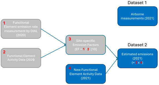
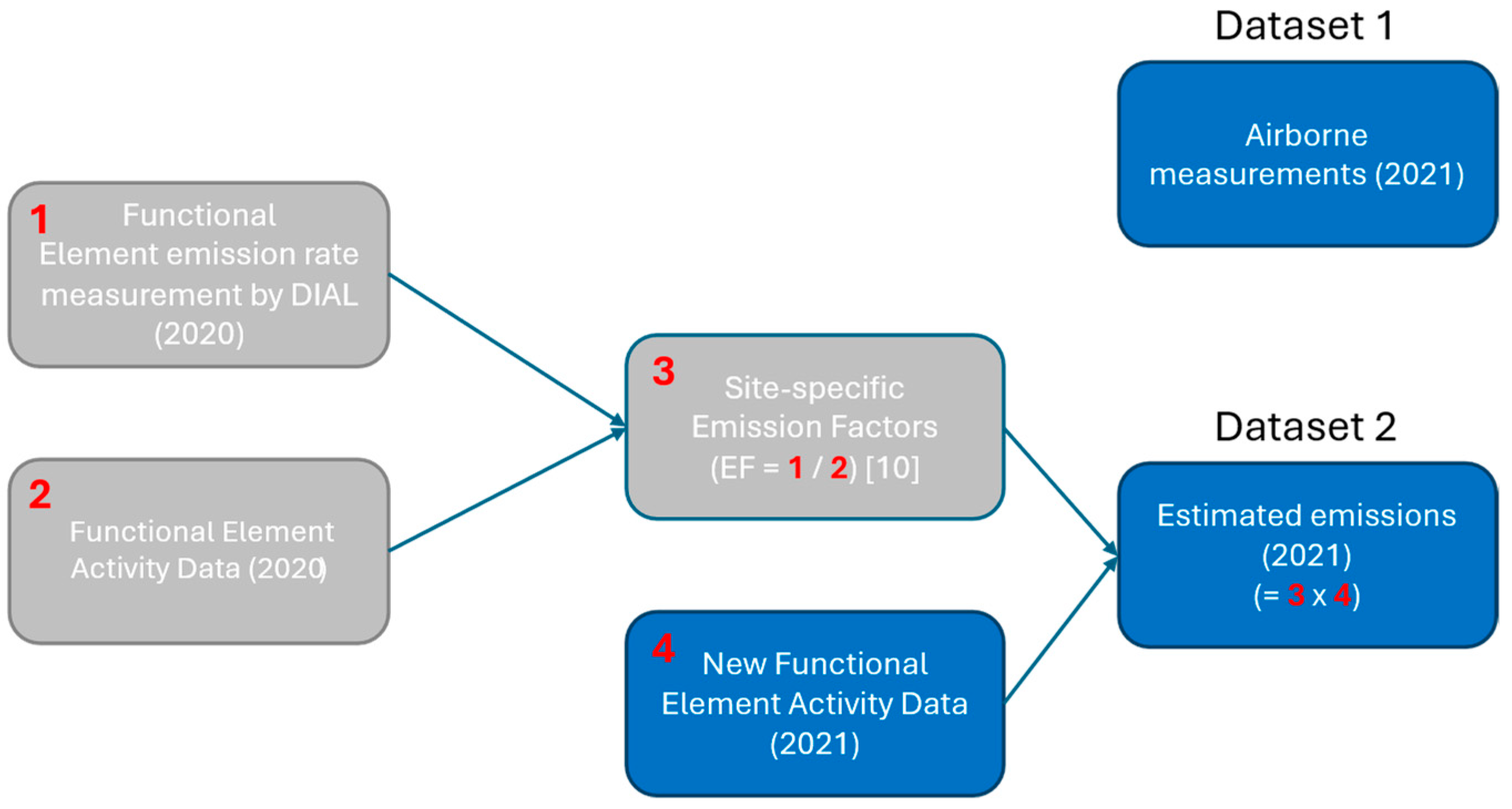
In this case study, one dataset is that of the measured total site emissions from the airborne method and the other is that of estimated total site emissions during this period. The estimated emissions dataset was calculated using FE EFs derived from DIAL measurements which were made approximately one year prior. It should be noted that the comparison is not of the two measurement datasets, rather the DIAL measurements provide the source data for the estimation dataset. This is akin to other EF resources used for emission rate estimation, for example EN 15446:2008 [29], with source data generated many years prior to subsequent use. To estimate the site emissions, the AD for each FE was obtained from the sites pertaining to the period of the airborne measurements. For each FE the AD was then combined with the EF previously reported to calculate an estimated emission rate at the time of the airborne measurements. These were summed across the site to calculate the estimated total site emissions for each site. This calculation was performed for each of the three measurement days using the most specific AD possible. Figure 1 depicts a schematic flow chart of the data sources used in the generation of the datasets in this paper.

Figure 1. Schematic flow chart of data sources comprising the datasets for comparison in this paper. Arrows show the flow of data. Data sources numbered (red) to allow for a simplified equation showing how they are combined. Colours highlight the year of acquisition or calculation, grey: 2020, blue: 2021. Data source 3 from Innocenti et al. [10].

A brief description of the important concepts used in this paper is included here. More detailed information can be found in the previous publication [10]. Firstly, the functional element (FE) concept refers to a unit or area of a site which is spatially separable and related to a specific process. Secondly, an emission factor (EF) is a value which relates the quantity of emissions from a source to another metric associated with that source. Finally, activity data (AD) is the metric of the source to which the EF is applied to calculate the estimated emissions. The EF and AD concepts are routinely used for emission reporting (e.g., to inventories).

In the majority of cases, the FE throughput has been used by Innocenti at al. [10] as the AD from which to calculate the estimated emission rate. However, there were some FEs for which the throughput was not deemed to be the most appropriate metric and an alternative has been used. It was found that emissions from the storage FE were not strongly correlated with the throughput and therefore throughput was not deemed to be the appropriate AD metric. Emissions were measured from storage FEs where no significant throughput was recorded whilst no emissions were measured from others with high throughput. As discussed by Innocenti et al. [10], the EF by number of storage FEs is a more appropriate metric and this is what has been used in this work to estimate the emissions from these FEs. The transfer jetty emission during ship loading activities was also found to be independent of the throughput. Similar emission rates were measured during high and low loading rates at each transfer jetty. Given the apparent independence of the transfer jetty emission rate to the throughput, the absolute mass emission rate previously measured has been used in this work as the estimate of the emission from this FE. There is an unknown level of uncertainty associated with this approach as it is not known how different ships or ship operators affect the emissions during ship loading activities.

The IPCC inventory reporting guidelines includes advice on the choice of EFs. Although provision is included for direct measurement of emissions and for EFs to be determined through measurement, it is recognised that it is common for inventories to be compiled using default EFs, EFs obtained from available literature or the IPCC Emission Factor Database. It is acknowledged within the guidance that some emission types are poorly or uncorrelated with throughput and relies on the assumption that the agreement improves with a large sample size. This may be a suitable approach for emission reporting across a large number of sites, but it highlights the need for specific emissions data when estimating emissions from an individual site.

A second dataset of the expected emissions was produced, taking into account the estimated effect of changes to the equipment, for example through maintenance, as indicated by the site operator. For FEs where the site has indicated an expected change in the emissions, these new expected emission rates have been used in the second dataset. However, whilst some assessment of this effect may have been performed by the site operators, it has not been rigorously determined and therefore a large uncertainty was applied, similar to inventory calculations for categories with large unknowns. In these cases, an uncertainty of 50% has been applied to the new, expected emission rates. The adjustment to the emission rate was set at the midpoint of the expected effect with a 50% uncertainty covering a range from 0 to 100% of the reported effect. This covers all scenarios from the worst case that there was no effect of the maintenance to the best case that the full expected reduction is achieved. It is not known how any other routine/daily maintenance work performed at the sites since the measurements from which the EFs were derived may have affected the emission profile of each FE. Similarly, the potential emergence of new sources is also an unknown factor with the opposite effect of increasing the emission rate. The solutions to improve these uncertainties to be more representative and achieve agreement between datasets would be: (1) Obtain up-to-date site-specific FE EFs close to the time the whole-site measurements are carried out. (2) Use EFs for each FE from the average of a large dataset from different sites that use similar technologies. The uncertainty or spread of each EF should encapsulate the different maintenance stages of the different sites and would address some of the uncertainty unaccounted for in this paper. (3) Compare over a statistically large sample size. This would randomise and minimise the uncertainties since the estimated emission of each FE emission may be larger at one site and smaller at another. This last point (3) would compensate for potentially inaccurate EFs by measuring multiple sites to achieve agreement. This is a similar concept to using an immature measurement technique, without a fully characterised uncertainty, measuring multiple sites to obtain a valid average emission rate with a representative uncertainty (e.g., for inventory purposes) but without valid measurements of each individual site. Conversely, obtaining bespoke FE EFs representative of the whole industry (as described in point (2)) would allow not only for these EFs to be applied at a regional/national scale for inventory purposes but also at a single site for the purpose of performing a reconciliation exercise.

However, the main limitation in this work associated with the estimation of methane emissions arises from the fact the EFs on which the estimates are based were derived from a small dataset with, for the most part, FEs measured in only one operational state. Therefore, a key assumption in this work is that the emission profile of an FE varies linearly with AD and it is not known whether this assumption is correct. This should not be an issue when the AD is approximately the same between the two techniques’ measurement periods. However, it is a potential source of uncertainty for the FEs wherein there is a significant difference in their AD. In this work, four FEs at each site (not necessarily the same FEs) exhibited a >30% difference in AD between the measurements used to derive the EFs and the airborne measurement period. The combined contribution to the site total emission rate from these FEs was 38% and 16% for sites L1 and L2, respectively.

It is worth considering that emission estimates generated for inventories or following existing standards, such as EN15446, rely on non-specific EFs, perhaps even to the industry let alone individual sites, with source data potentially decades old. Therefore, notwithstanding the limitations discussed, the use of site-specific EFs in this work, generated only one year before their use, should represent an improvement over existing approaches.

2.5. Sources of Uncertainty

The standard uncertainty of each DIAL measurement is estimated based on the standard deviation of the individual emission rate measurements from which each mean emission rate value is determined. As such it encapsulates variability occurring during the measurements which will include the measurement itself (random DIAL measurement uncertainty), variability in the source emissions, and variability in the wind direction and speed used, since for each scan a different wind profile is calculated from the wind data collected on-site. In previous validation studies, the standard uncertainty of a set of at least four DIAL scans has been shown to be representative of the measurement uncertainty. These studies also confirmed the dominant DIAL uncertainty sources display random behaviour, with the systematic biases in the DIAL-measured emission estimates being less than 4% [15,18]. When summing the emissions from different parts of the site which have been measured separately, for example when calculating total site emissions, the reported standard uncertainty is the sum in quadrature of the standard uncertainties of each contributing measurement. Such total uncertainty is relatively low when compared to a single DIAL measurement. This is expected for methods where the dominant uncertainty sources have a random behaviour since, by increasing the number of measurements (and scans), the uncertainty can be expected to decrease accordingly.

The standard uncertainty of the AD was derived from on the standard deviation of the timeseries of AD values obtained during the measurement period used to calculate the EFs. To calculate the uncertainty in the EF, the uncertainty in the DIAL-measured emission rate and the uncertainty in the AD were propagated and expanded to a 95% confidence interval using two-sided t-statistic coverage factors as defined in the Joint Committee for Guides in Metrology’s (JCGM) Guide to the expression of uncertainty in measurement (GUM) [30]. The dominant source of uncertainty is the DIAL measurement uncertainty as reported by Innocenti et al. [10].

The uncertainty in the estimated emissions for each FE was calculated by propagation of the EF uncertainty with the uncertainty in the new AD. No attempt had been made to assess the uncertainty in the measurement of the AD used for the calculation of the EFs in the previous paper and the estimated emission in this work. While this is a source of uncertainty for the calculated EFs, it should be noted that any systematic uncertainty in the operator’s measurement of the AD or any correlated uncertainty between the two datasets would cancel out when calculating the estimated emissions. Where it was not possible to estimate the uncertainty in the AD, the uncertainty in the estimated FE emission rate was calculated by expanding only the EF uncertainty. As mentioned in the previous section, the effect of any unknown changes in the site (e.g., emergence of new sources) has not been included, albeit this could potentially be estimated through modelling. For a site with a good maintenance programme, it is statistically likely that the emergence of new sources is balanced by repair of existing ones.

To calculate the estimated emissions for the total site, the individual FE-estimated emissions were summed. The respective uncertainties were summed in quadrature to calculate the uncertainty of the site total estimated emissions.

The method of estimating the site total emissions through the summation of many individual (FE) emission estimates is similar to that used for national inventories. The result, in both cases, is a low uncertainty for the overall estimate despite large unknowns (e.g., for the EF) and large relative uncertainties for the constituent parts (e.g., FE or inventory categories). This arises due to the many independent emission sources comprising the total, providing a large possibility for compensation between sources. That is to say that an underestimate in the emission estimate for one constituent part is likely to be compensated by an overestimate in the emission estimate of another. It is improbable that all constituent estimates are equally incorrect in the same way so as to create a large positive or negative bias in the total. The effect is that, whilst the estimates for individual FEs or inventory categories may be significantly inaccurate with large uncertainties, the total can be expected to be reliable with a representative, and possibly low, uncertainty. The suggestions made in this paper to improve the EFs would provide more representative FE emission values and uncertainties; however, the overall uncertainty of the total will remain relatively low.

In calculating the average estimated emission rate over the three airborne measurement days, the estimated emissions for each FE were weighted according to the number of airborne measurement curtains on the corresponding day. The standard uncertainty for each FE was weighted in the same way when calculating the uncertainty of this value.

A literature review was conducted to assess the possible uncertainty sources and magnitude from airborne emission curtain measurements, similar to those conducted which are included in this work. There are predominately two main approaches to emission rate quantification from such curtain-type airborne measurements. One is a single-curtain approach, where each the emission rate calculated for each curtain is reported as an individual measurement. The other is a multi-traverse/curtain approach, where the reported emission rate measurement is the average of data across multiple flights. The uncertainty assessment has only included literature pertaining to a curtain-type measurement approach as it is most similar to the measurements included in this paper. Other flight measurement approaches, such as box approaches, are not included.

In this work the single-curtain approach was employed to calculate and report the site emission rate, with each of the seven flight curtains reported as a measurement, as reported in Table 1. An assessment of the uncertainty of the single-curtain approach is given by Cambaliza et al. [31]. Cambaliza et al. identify a number of variables in this approach as introducing a significant contribution to the uncertainty, including: the determination of the background concentration, the boundary layer height, the lack of data between the lowest altitude transect and the surface, and the process of interpolation between the ground and lowest transect. Hacker et al. [23] report that a minimum transect altitude of 15 m should only introduce minimal uncertainties, whilst implying that at 150 m the effect could be significant. During the measurements of the LNG sites, the minimum transect altitude was between 60 and 95 m, which could be a significant source of uncertainty. The conclusion drawn by Cambaliza et al. is that the uncertainty in the single-curtain method is conservatively estimated at 50%, although this is actually the maximum relative difference of repeated measurements.

Table 1. Relative methane emission rate for sites L1 and L2 measured by ARA’s airborne method.

Measurement Day	Traverses (#)	Site L1	Site L2	Sites L1 + L2
1	12	0.90	1.66	1.45
	9	0.65	1.30	1.11
2	13	0.53	1.27	1.06
3	11	0.47	0.77	0.68
	3	0.50	1.11	0.94
	5	0.49	1.08	0.91
	9	0.66	1.03	0.92

# indicates the number of traverses performed.

An alternative approach, averaging data across multiple flights, is described in an ESA report [24] which subsequently forms the basis of a scientific paper by Krings et al. [25]. These works contain a detailed discussion on the measurement and calculation approach including a rough sensitivity analysis of some of the parameters affecting the mass emission rate calculation, arriving at a value of 10% uncertainty, predominantly based on variability in the wind speed. The level of confidence in this uncertainty is not stated. The method described by Krings et al. averages the data at the grid cell (bin) level from multiple traverses at the same elevation across different flight curtains. A measurement comprises a (non-defined) number of repeat traverses/curtains. As mentioned by Krings et al., to achieve the stated estimated uncertainty of 10%, many repeats are needed to randomise sources of uncertainty. This uncertainty estimate does not include any systematic uncertainty.

For this paper it was not possible to exactly replicate the method described by Krings et al., averaging multiple traverses of the same elevation, as only data at the curtain level was available. Nonetheless, averaging the seven flight curtains from the ARA measurements should yield something equivalent to the method described by Krings et al. with a comparable uncertainty. This will be discussed further in the Results and Discussion Sections (Section 3 and Section 4).

From the available literature it can be concluded that the uncertainty of a single curtain is likely to be high. This approach requires a full uncertainty budget assessing all the variables and sources of uncertainty. Averaging data from multiple flights could result in uncertainties as low as 10%, albeit the level of confidence is not stated, nor is the required sample size. This approach provides a statistical assessment of the uncertainty from repeat curtains. It does not, however, include any systematic uncertainty, without validation of the methodology. In either case, a high minimum transect altitude and the extrapolation of the plume profile to the ground are potentially significant sources of uncertainty.

3. Results

This paper would not be possible without the cooperation of the site operators and it is required to maintain their anonymity. To that end, all results presented here have been normalised with respect to the absolute mass emission rate measured by DIAL in 2020 at each site. The normalised data has the added benefit of implicitly providing a comparison with the absolute mass emission rates measured by DIAL, which is equal to 1.

Table 1 presents the relative emission rates measured using ARA’s airborne measurement method for each site. For the majority of the Fes, the throughput across the three flight measurement days was stable and consistent with a maximum variation over the 3 days for each FE, with <20% for site L1 and <10% for site L2. However, more importantly, the estimated site total emission rates for both sites does not change significantly across the three days with a maximum variation of 5% and 4% for site L1 and L2, respectively. From this it can be deduced that the site can be expected to exhibit stable emissions across the three days. The site operators also confirmed the stability of the operations and that no emission events were known of. Any variation in the reported emission rates between flight curtains is therefore predominately due to variability in the technique rather than the source and we cannot infer source variability whether present or not.

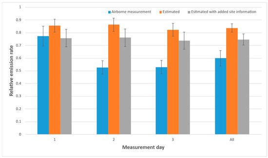
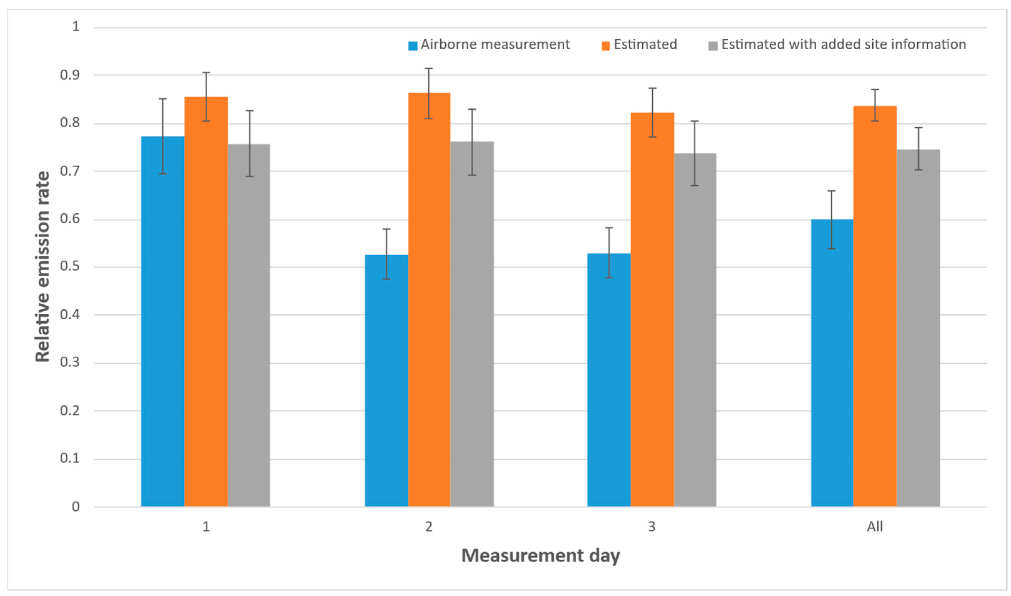
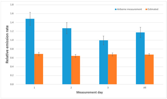
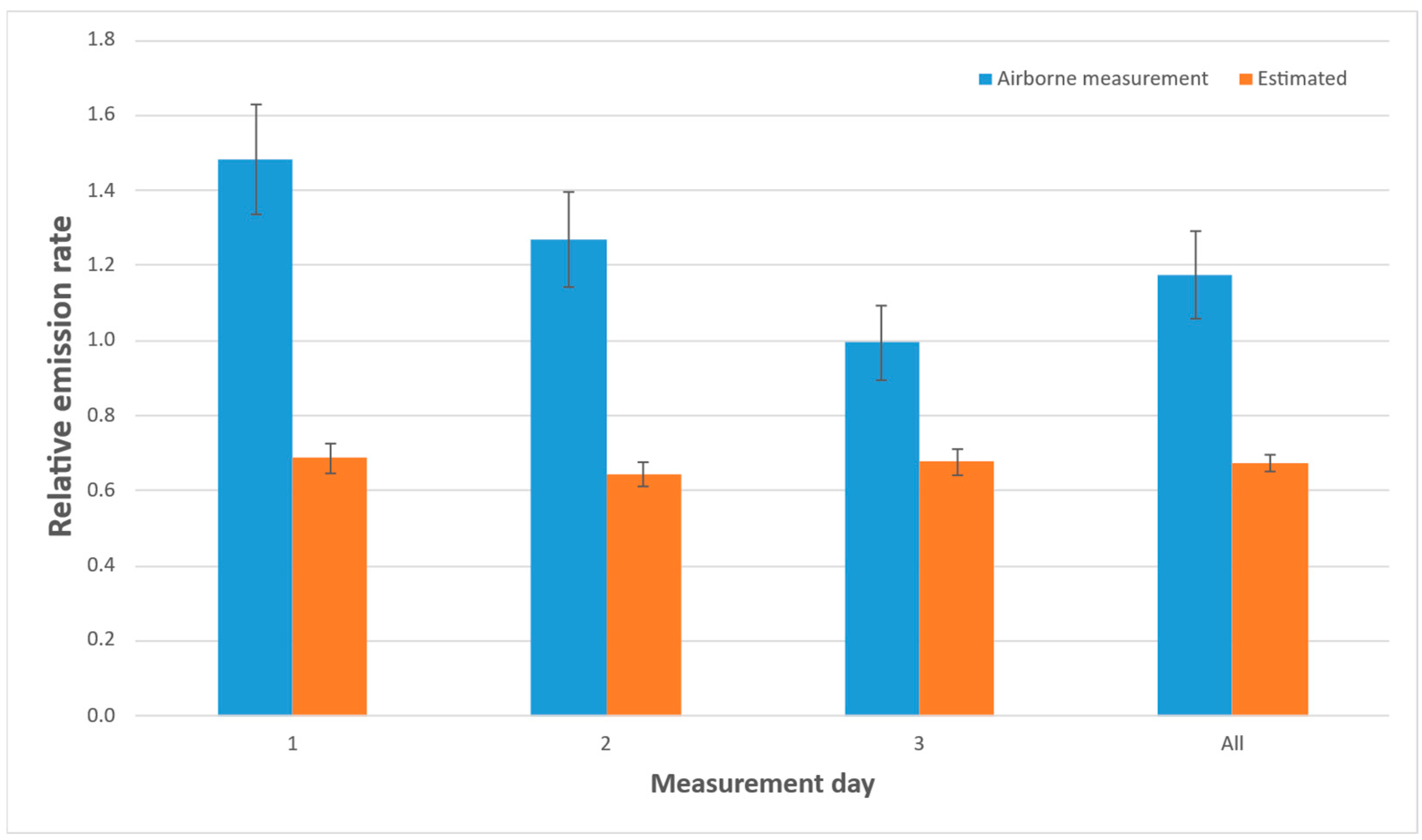
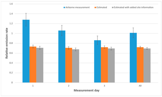
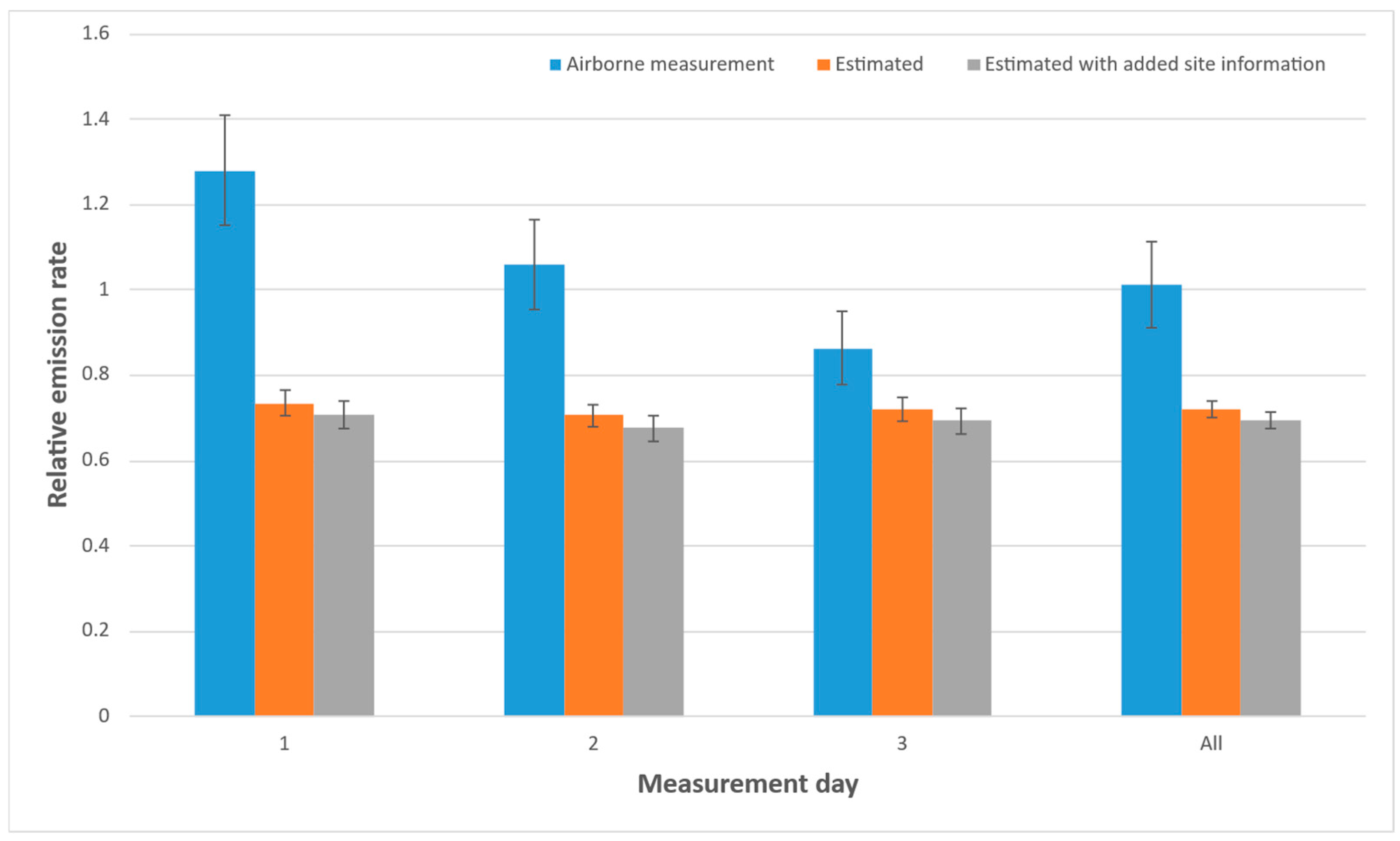
Figure 2 and Figure 3 present the relative emission rates for sites L1 and L2, respectively, measured by the airborne technique and estimated using the EFs and AD. The data has been averaged for each flight measurement day and across all measurement days. To account for the different number of airborne measurements on each day, the estimated emission rates for the average across all days has been weighted. For site L1 the site operators provided extra information on the expected emissions from select FEs which had undergone repair or maintenance, which are taken into account in a second dataset. No such maintenance work was performed at site L2 and as such a second dataset was not created. The uncertainties presented in Figure 2 and Figure 3 for the estimated emissions are at a 2-sigma level of confidence. These have been calculated by propagating the standard uncertainties and expanding using a two-sided t-statistic distribution, giving a 95% confidence value. As it is not possible to review all the uncertainty sources associated with the flight measurements, the uncertainty of a single curtain is not available. Instead, a minimum uncertainty of 10% has been applied to each airborne measurement curtain as a reference only and is likely an underestimate. It has been assumed that this uncertainty in the airborne measurements is also at a 2-sigma level of confidence, although this is not clear and it will be discussed later in the paper.

Figure 2. Relative methane emission rates for site L1 averaged for each measurement day. Airborne measurement (blue), estimated site total (orange) and estimated site total with added site information (grey).

Figure 3. Relative methane emission rates for site L2 averaged for each measurement day. Airborne measurement (blue) and estimated site total (orange).

Agreement between datasets should only be defined by overlapping uncertainty confidence intervals, albeit where an overlap is due to large uncertainties the usefulness of an agreement is diminished. This definition relies on validated uncertainties for both datasets. Where one or both datasets have non-validated uncertainties, as in this case, this definition is not applicable. Instead, it is practical to observe the difference between datasets and, from the non-validated uncertainties, whether agreement could be considered to be relatively close or not. Figure 2 and Figure 3 show that for both sites the airborne measurements are variable between measurement days (38% and 39% maximum difference between days for site L1 and L2, respectively), whilst the estimated emissions are constant (5% and 6% maximum difference for site L1 and L2, respectively). For site L1, agreement has appeared to have been achieved for day 1; however, day 2 and 3 exhibit differences of 33% and 28%, respectively, between the uncertainty limits of the airborne measurement and the estimated emissions. This indicates a high degree of uncertainty for an individual flight measurement curtain and that the measurement has been under-sampled in terms of repeat curtains; however, through repeat sampling the uncertainty of the average may become representative of the measurement.

It was noted by the flight operator that there could be a source of methane in the region upwind of the sites. Given the site locations, the location of the potential upwind source, and the wind conditions at the time of measurement, any potential upwind source would predominantly affect site L1. Upwind sources should be accounted for at the measurement stage, for example by choosing measurement conditions which exclude such sources or through measurement and subtraction of upwind contributions. In this case, site L1 would be primarily affected and removing any upwind methane contribution would lead to a lower likelihood of agreement between the datasets.

The airborne measurements were performed for both sites during a single measurement curtain with site separation achieved during the data analysis stage. It may be that perfect separation of the sites was not always possible, which could explain the difference between the sites, in that the airborne measurements for L1 are lower than estimated whilst for L2 they are higher. The total, L1 + L2 would be unaffected. Figure 4 presents the results of the combined total of sites L1 + L2. Values for the estimated L1 + L2 dataset were calculated by summing the values for the individual sites and normalising by the total mass emission rate measured by DIAL for both sites. As for Figure 2 and Figure 3, the uncertainties presented in Figure 4 for the estimated emissions are expanded uncertainties at a 2-sigma level of confidence. The uncertainty in the airborne measurements is 10%, as a reference only, which has been assumed to be at the same, 2-sigma confidence level.

Figure 4. Relative methane emission rates for site L1 + L2 averaged for each measurement day. Airborne measurement (blue), estimated site total (orange), estimated site total with added site information (grey).

4. Discussion

The uncertainty in the estimated emission rates is calculated from the propagation of the uncertainty in the DIAL measurements underpinning the EFs and the site AD. The dominant source of quantifiable uncertainty in the estimate is the contribution arising from the DIAL measurements. The main limitations in the estimation of the site emission rates have been discussed in Section 2.4. These are the assumption of linearity in the EFs with respect to AD and the potential change in the emission profiles between the derivation of the EFs and the subsequent airborne measurements (e.g., unbalance between the repair of old sources and the emergence of new sources). For these reasons, the reported emission rates could have extra systematic uncertainties which would either increase or decrease these values.

As mentioned, a full review of the uncertainty sources is not possible and a 10% uncertainty is applied initially as a reference. However, the high variability between repeat flight curtains observed in this work supports the findings from Cambaliza et al. that the uncertainty of individual flight curtains is high, particularly when considering the variability between consecutive flights on a single day where the site emissions are not expected to vary. For example, for site L1 on day 1 the two measurements showed a variability of 32% when compared to the average value. These two measurements were made within two hours of each other over a period where all the AD values were constant with the site, confirming the operations were stable and there were no known emission events. This variation must predominantly be due to technique variability and the uncertainty in a single curtain should therefore be expected to be higher than 10%, although, as mentioned, there is ongoing work to improve the uncertainty assessment [28]. A high uncertainty for a single quantification (in this case a curtain) should not be considered an issue in itself and is likely common between atmospheric emission measurement techniques where uncertainties related to wind are likely a dominant factor. Rather, this can highlight the requirements for the method to constrain the uncertainty, for example by defining a measurement as the average of a set number of repeats.

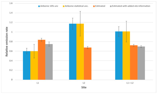
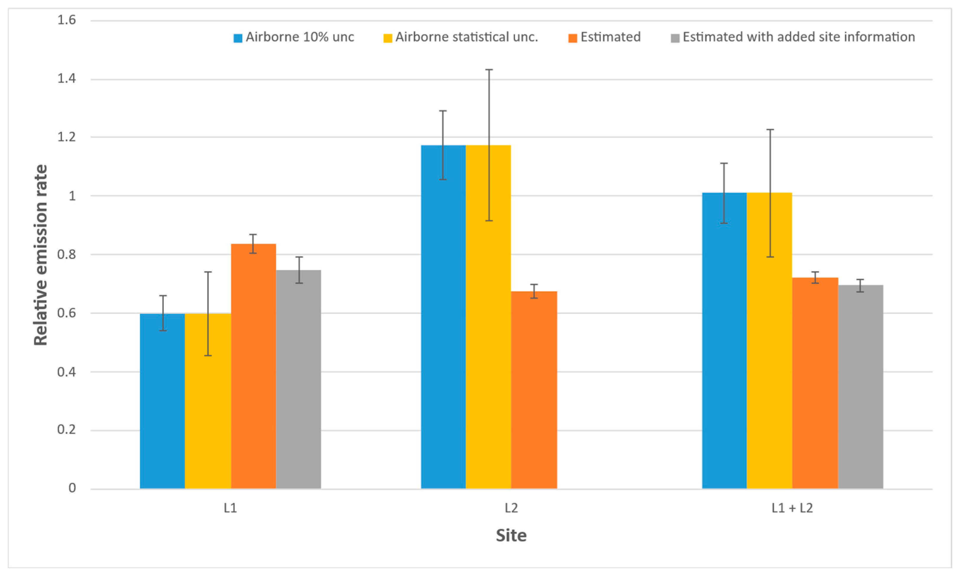
The uncertainty of the airborne method can also be assessed statistically using the standard deviation across a set of flight measurement curtains in the same way as described for the DIAL method to report a 95% confidence level using a two-sided t-statistic distribution. Figure 5 presents the average relative methane emission rates for each site across all measurement days and includes the airborne measurement method with the expanded uncertainty from the statistical uncertainty analysis. These uncertainties are 24% for site L1 and 22% for site L2 and sites L1 + L2. Assessing the uncertainty in this way includes the random uncertainty arising from variability in the technique captured by the distribution of values across the repeat measurements. This is similar to the calculation method described by Krings et al., although involves averaging at the whole-curtain level as opposed to the grid-cell level. The expanded uncertainties from the ARA flights also compare well with the Krings et al. calculation of 10% assuming this was a standard uncertainty (1 sigma) rather than the expanded uncertainty (2 sigma). This shows the potential to achieve relatively small uncertainties for an average measurement. Improvements in the methodology, for example with the minimum transect altitude and extrapolation approach, could reduce the uncertainties further.

Figure 5. Relative methane emission rates averaged across all measurement curtains. Airborne measurement (blue), airborne measurement with statistical uncertainty assessment (yellow), estimated site total (orange), estimated site total with added site information (grey).

Conducting the same statistical uncertainty analysis for the individual measurement days gives an expanded uncertainty of 209% and 157% for day 1 at sites L1 and L2, respectively. This indicates that the sample size of two curtains, and implicitly a single curtain as on day 2, is insufficient for the purpose of individual site quantification and dataset comparison. The approach of using a single or a small number of curtains may work well for inventory reporting purposes across many sites if the sample size is sufficiently large and the validated methodology was proven to be dominated by random uncertainties. However, this cannot be demonstrated within the scope of this paper. For day 3 the statistical expanded uncertainty for sites L1 and L2 is 25% and 26%, respectively, showing an improvement with an increased sample size of four curtains. It should be noted that without a proper validation of the methodology it is not known whether the statistical uncertainty presented in Figure 5 is representative of this method’s true uncertainty. This uncertainty assessment does not account for any systematic uncertainty which may be present that increases the overall uncertainty. A validated method should seek to address any potential source of systematic uncertainty.

Figure 5 shows that for site L1, the average of the airborne measurements and the estimated emissions with the added site info agree within the statistical uncertainties. This cannot be said for site L2 or for the combined site L1 + L2 measurements, with differences of 27% and 10%, respectively, between the uncertainty limits, although the latter is close. This could, in part, be caused by the limitation previously discussed of the estimation method. For example, non-linearity may exist between the AD and emission rate profile for some FEs leading to incorrect emission estimates. Any FE which exhibits a large difference in AD between the measurements used to derive the EF and subsequent measurements would benefit from confirmation of the EF at different AD values. This would be similarly beneficial for an FE which can be operated in multiple modes. FEs which have potentially been included in a maintenance programme would benefit from updated EFs to assess the effect of such maintenance. These issues could be addressed through calculation of FE EFs from the average of a sufficiently large dataset across multiple sites which use similar FE technologies. The average EFs would, statistically, cover FEs with varying states of maintenance and across different AD values. Alternatively, comparison over a statistically large enough sample size of sites would minimise the aforementioned issues as potential over- or underestimations of FE emissions would compensate for each other. In this case, the comparison would only be applicable over the entire sample and a comparison at the individual site level would not be possible.

As discussed in Section 2.5, the summation of individual FE emission estimates to calculate a site total can result in a relatively small uncertainty for the total estimate despite potentially large uncertainties for individual FE estimates due to the possibility for uncertainty compensation. This can be seen in Figure 5, where the total for ‘Estimated with added site information’ (grey bar) includes a number of FEs with a large uncertainty, reflecting the unknown effect of maintenance (see Section 2.4). Despite this, the uncertainty of the total is 5.9% and 2.9% for L1 and L1 + L2, respectively, compared to uncertainties of 4.0% and 2.6% for the ‘Estimated’ (orange bar) total of L1 and L1 + L2, respectively, where the uncertainties of these FEs are not as large. Considering these two main limitations, the estimated emission rates could have extra systematic uncertainties that could either increase or decrease the reported values while maintaining the same uncertainty derived from the EF calculations. On the other hand, the uncertainty of the airborne measurement is not well characterised and could also be underestimated even when the statistical analysis is considered. Given the relatively high variability between the emissions from different curtains in the airborne technique, it could be that the measurement has been under-sampled in terms of sample size and that an increase in the number of repeats may have led to greater agreement with reduced uncertainty. Improvements to the flight technique methodology have the potential to increase the agreement between the datasets. As described the method used in this work does not apply a correction to account for the flight traverse heading deviation from normal with the wind direction, flying at lower elevations, and the choice of an extrapolation method based on an assessment of the plume profile could have a significant effect on the calculated flux. Nevertheless, the datasets are close to agreement.

The difference in the magnitude of the uncertainties presented has no relation to the spatial scale of the measurement technique. That is, it is not correct to assert that site-level techniques are less certain than more granular techniques. Notwithstanding the limitations in the estimated data already mentioned, the primary driver of the difference in the magnitude of the uncertainties is the maturity of the underpinning measurement methodologies involved in this type of comparison.

This work has shown the potential of using estimated methane emissions from EFs derived for each FE and it has also highlighted the limitations of the currently available datasets. While the estimated emissions and site-level data are close to agreement, the use of fully validated methodologies, up-to-date EFs and a larger sample of EFs, both at different AD values and from a large sample at different liquefaction facilities, would significantly improve these types of comparisons by producing representative uncertainties for both estimated and measured emissions. These challenges are not specific to this case study and would apply to any reconciliation exercise, including those conducted under the OGMP 2.0 framework. For example, using fully validated methodologies could support informed interpretations of systematic trends in the data. In this case, it might have been possible to confidently speculate whether the site-level measurement missed emissions at L1 (see Figure 2) or if the EF-based estimates missed emissions at L2 (see Figure 3).

5. Conclusions

The reconciliation exercise case study presented in this paper, comparing a measurement-based emission estimate with site-level measurements, highlighted several challenges which could lead to non-comparable datasets if not properly addressed.

Achieving agreement between datasets could be possible using two validated measurement methodologies and measuring at the same time. A validated methodology should include, at minimum, a definition of the measurement output (e.g., the number of repeats required and under what conditions) and well defined quality assurance and quality checks to exclude invalid or highly uncertain data. The set of these procedures should then be demonstrated to produce validated measurements with an associated uncertainty representative of the estimated emissions. Only through such a validation process can confidence be had in the datasets and therefore the reliability of the comparison. For sites such as LNG facilities where high emissions of carbon dioxide (CO₂) are also present, measurements of CO₂ could help to assess the performance of a methodology and highlight potential sources of bias or uncertainty by providing an independent reference source, as reported by Lunt et al. [28].

To obtain accurate estimates of individual FEs, EFs must be kept up to date and reflect, as closely as possible, the current state of the site at the time of the measurements. Where a long period of time has elapsed between the source measurements from which the EFs are derived and the site measurements, changes to the site may have occurred (e.g., maintenance and new sources) which may render the EFs no longer fully representative. This is only an issue if knowledge of the emissions from individual FEs is important. Agreement between datasets can be achieved at a site or multi-site level with relatively low uncertainty in the estimate where the estimate is the summation of many constituent parts (e.g., FEs). In this case the emission estimates for the FEs may not be accurate and have large associated uncertainties which are, however, likely to compensate for each other. The biggest improvement that can be made, for any reconciliation exercise, is having a statistically large dataset from which to derive EFs, capturing FEs under different and representative AD. After major maintenance of an FE, a new EF should be derived through measurement with a validated method.

It is important to identify the purpose of any measurement and subsequent reconciliation exercise as this will guide the requirements and level of maturity of the measurement methodology and the process for calculating EFs. This work tries to achieve agreement between datasets at the site level, with only one validated measurement methodology and EF derived from a small sample size. Given this, it is expected that achieving such agreement is unlikely; however, the potential is shown if datasets were larger and methodologies developed. Further work is ongoing to improve the flight measurement methodology used in this work.

This paper shows the potential of using site-specific, FE-based EFs to estimate total site methane emissions for the purpose of comparison between measurement datasets. The use of site-specific EFs, based on recent source data, should represent an improvement compared to existing emission estimation approaches. In this case study the FE scale is at a more granular level when compared to the whole-site measurements obtained using the airborne method; however, the approach is valid for any dataset comparison including an OGMP 2.0 framework level-5 reconciliation. A reconciliation exercise within the OGMP 2.0 framework will encounter the same challenges around method validation and uncertainty assessment as presented in this paper, albeit it could be that it is the more granular dataset which is less well defined. As demonstrated in this work, thought must be given towards the representativeness of the uncertainty estimates, as well as the unquantified (or unquantifiable) uncertainties as part of the reconciliation exercise. Through this case study the challenges and limitations on the datasets are identified and discussed. This is pertinent as any reconciliation exercise is likely to encounter similar challenges, including incomplete datasets with unvalidated or no uncertainty. This study is, therefore, a good representation of a real reconciliation exercise. Two complete datasets with perfectly characterised uncertainties would be an ideal scenario and likely improve the chances of dataset agreement. Thus, by highlighting these issues through this work and suggesting routes to improvement, greater value and meaning could be gained from future exercises.

Whenever the results of a reconciliation exercise do not achieve agreement between datasets, an opportunity is presented to understand the causes and aim to improve the results with a future reconciliation exercise. This would enable operators to improve the understanding of their facility emission profile, which is related to operations. In turn this enables targeted maintenance and repair programmes, thus focusing resources where they can have the biggest impact in decreasing the emission footprint, which should be the final aim of any measurement campaign.

References

- Chapter 7: The Earth’s Energy Budget, Climate Feedbacks and Climate Sensitivity. Available online: https://www.ipcc.ch/report/ar6/wg1/downloads/report/IPCC_AR6_WGI_Chapter07.pdf (accessed on 10 June 2026).
- The Paris Agreement | UNFCCC. Available online: https://unfccc.int/process-and-meetings/the-paris-agreement (accessed on 22 June 2023).
- World—World Energy Balances: Overview—Analysis. Available online: https://www.iea.org/reports/world-energy-balances-overview/world (accessed on 22 June 2023).
- Statistical Review of World Energy 2025. Available online: https://www.energyinst.org/statistical-review (accessed on 10 June 2026).
- Zhang, X.; Myhrvold, N.P.; Hausfather, Z.; Caldeira, K. Climate Benefits of Natural Gas as a Bridge Fuel and Potential Delay of Near-Zero Energy Systems. Appl. Energy 2016, 167, 317–322. [Google Scholar] [CrossRef] [Scilit]
- The Role of Gas in Today’s Energy Transitions—Analysis. Available online: https://www.iea.org/reports/the-role-of-gas-in-todays-energy-transitions (accessed on 30 September 2020).
- Brandt, A.R.; Heath, G.A.; Cooley, D. Methane Leaks from Natural Gas Systems Follow Extreme Distributions. Environ. Sci. Technol. 2016, 50, 12512–12520. [Google Scholar] [CrossRef] [Scilit] [PubMed]
- OGCI-Guidance-on-Near-Zero-Methane-Emissions.Pdf. Available online: https://www.ogci.com/wp-content/uploads/2023/08/OGCI-guidance-on-near-zero-methane-emissions.pdf (accessed on 10 June 2026).
- IGU World LNG Report 2022. Available online: https://www.igu.org/igu-reports/world-lng-report-2022 (accessed on 10 June 2026).
- Innocenti, F.; Robinson, R.; Gardiner, T.; Howes, N.; Yarrow, N. Comparative Assessment of Methane Emissions from Onshore LNG Facilities Measured Using Differential Absorption Lidar. Environ. Sci. Technol. 2023. [Google Scholar] [CrossRef] [Scilit]
- Publications—IPCC-TFI. Available online: https://www.ipcc-nggip.iges.or.jp/public/2006gl/index.html (accessed on 22 June 2023).
- ENVIRONMENTAL PROTECTION AGENCY—Greenhouse Gas Reporting Rule: Revisions and Confidentiality Determinations for Petroleum and Natural Gas Systems. Available online: https://www.govinfo.gov/content/pkg/FR-2023-08-01/pdf/2023-14338.pdf (accessed on 10 June 2026).
- Regulation—EU—2024/1787—EN—EUR-Lex. Available online: https://eur-lex.europa.eu/eli/reg/2024/1787/oj/eng (accessed on 4 August 2025).
- Mineral Methane Initiative OGMP2.0 Framework. Available online: https://www.ogmpartnership.org/sites/default/files/resources/2025-04/OGMP_20_Reporting_Framework.pdf (accessed on 10 June 2026).
- Innocenti, F.; Robinson, R.; Gardiner, T.; Finlayson, A.; Connor, A. Differential Absorption Lidar (DIAL) Measurements of Landfill Methane Emissions. Remote Sens. 2017, 9, 953. [Google Scholar] [CrossRef] [Scilit]
- Robinson, R.; Gardiner, T.; Innocenti, F.; Woods, P.; Coleman, M. Infrared Differential Absorption Lidar (DIAL) Measurements of Hydrocarbon Emissions. J. Environ. Monit. 2011, 13, 2213–2220. [Google Scholar] [CrossRef] [Scilit] [PubMed]
- Innocenti, F.; Gardiner, T.; Robinson, R. Uncertainty Assessment of Differential Absorption Lidar Measurements of Industrial Emissions Concentrations. Remote Sens. 2022, 14, 4291. [Google Scholar] [CrossRef] [Scilit]
- Gardiner, T.; Helmore, J.; Innocenti, F.; Robinson, R. Field Validation of Remote Sensing Methane Emission Measurements. Remote Sens. 2017, 9, 956. [Google Scholar] [CrossRef] [Scilit]
- Howes, N.; Finlayson, A.; Smith, T.; Innocenti, F.; Robinson, R.A. CEN/TC 264/WG 38: “Determination of Diffuse VOC Emissions”. Available online: https://www.vdi.de/fileadmin/pages/vdi_de/redakteure/ueber_uns/fachgesellschaften/KRdL/dateien/WG_38_Final_Report_SACEN2014-07.pdf (accessed on 10 June 2026).
- Pikelnaya, O.; Polidori, A.; Tisopulos, L. Controlled Release. Available online: http://www.aqmd.gov/ors-study/controlled-release (accessed on 28 June 2023).
- EN 17628:2022; Fugitive and Diffuse Emissions of Common Concern to Industry Sectors—Standard Method to Determine Diffuse Emissions of Volatile Organic Compounds into the Atmosphere. European Committee for Standardization (CEN): Brussels, Belgium, 2022. Available online: https://standards.iteh.ai/catalog/standards/cen/1134347e-e278-42cd-9967-2a4f34ac0fe6/en-17628-2022?srsltid=AfmBOoryhz5shr8N8YfD7JXNVkZbzMRXG_ZLBTPGTNRhmc0F_TpfQtvN (accessed on 10 June 2026).
- Erland, B.M.; Adams, C.; Darlington, A.; Smith, M.L.; Thorpe, A.K.; Wentworth, G.R.; Conley, S.; Liggio, J.; Li, S.-M.; Miller, C.E.; et al. Comparing Airborne Algorithms for Greenhouse Gas Flux Measurements over the Alberta Oil Sands. Atmos. Meas. Tech. 2022, 15, 5841–5859. [Google Scholar] [CrossRef] [Scilit]
- Hacker, J.M.; Chen, D.; Bai, M.; Ewenz, C.; Junkermann, W.; Lieff, W.; McManus, B.; Neininger, B.; Sun, J.; Coates, T.; et al. Using Airborne Technology to Quantify and Apportion Emissions of CH4 and NH3 from Feedlots. Anim. Prod. Sci. 2016, 56, 190. [Google Scholar] [CrossRef] [Scilit]
- Scientific and Technical Assistance for the Deployment of a Flexible Airborne Spectrometer System During C-MAPExp. Available online: https://earth.esa.int/eogateway/documents/20142/37627/C-MAPExp-Final-Report.pdf (accessed on 10 June 2026).
- Krings, T.; Neininger, B.; Gerilowski, K.; Krautwurst, S.; Buchwitz, M.; Burrows, J.P.; Lindemann, C.; Ruhtz, T.; Schüttemeyer, D.; Bovensmann, H. Airborne Remote Sensing and In-Situ Measurements of Atmospheric CO2 to Quantify Point Source Emissions. Atmos. Meas. Tech. 2016, 11, 721–739. [Google Scholar] [CrossRef] [Scilit]
- Borchardt, J.; Harris, S.J.; Hacker, J.M.; Lunt, M.; Krautwurst, S.; Bai, M.; Bösch, H.; Bovensmann, H.; Burrows, J.P.; Chakravarty, S.; et al. Insights into Elevated Methane Emissions from an Australian Open-Cut Coal Mine Using Two Independent Airborne Techniques. Environ. Sci. Technol. Lett. 2025, 12, 397–404. [Google Scholar] [CrossRef] [Scilit]
- Harris, S.J.; Krautwurst, S.; Hacker, J.; Lunt, M.; Jakob, B.; Bai, M.; Boesch, H.; Brain, T.; Burrows, J.P.; Chakravarty, S.; et al. Evaluation of Coal Mine Methane Inventory Methods Using Aircraft-Based Approaches in the Bowen Basin, Australia. EGUsphere 2026. [Google Scholar] [CrossRef] [Scilit]
- Lunt, M.F.; Harris, S.J.; Hacker, J.; Joynes, I.; Robertson, T.; Thompson, S.; France, J.L. An Evaluation of Airborne Mass Balance and Tracer Correlation Approaches to Estimate Site-Level CH4 Emissions from LNG Facilities Using CO2 as a Tracer of Opportunity. Atmos. Meas. Tech. 2025, 18, 4413–4431. [Google Scholar] [CrossRef] [Scilit]
- EN 15446:2008; Fugitive and Diffuse Emissions of Common Concern to Industry Sectors—Measurement of Fugitive Emission of Vapours Generating from Equipment and Piping Leaks. European Committee for Standardization (CEN): Brussels, Belgium, 2008. Available online: https://standards.iteh.ai/catalog/standards/cen/ca30d7f9-a531-46eb-9ce1-5786a5270bf1/en-15446-2008?srsltid=AfmBOori6IynVEtYaVD0GyCG0zg6_Taz5AyJ2umSGOwwnVK0_WJ_g7hV (accessed on 10 June 2026).
- Guide to the Expression of Uncertainty in Measurement—Part 1: Introduction; Bureau International des Poids et Mesures (BIPM): Sèvres, France, 2023.
- Cambaliza, M.O.L.; Shepson, P.B.; Caulton, D.R.; Stirm, B.; Samarov, D.; Gurney, K.R.; Turnbull, J.; Davis, K.J.; Possolo, A.; Karion, A.; et al. Assessment of Uncertainties of an Aircraft-Based Mass Balance Approach for Quantifying Urban Greenhouse Gas Emissions. Atmos. Chem. Phys. 2014, 14, 9029–9050. [Google Scholar] [CrossRef] [Scilit]
Disclaimer/Publisher’s Note: The statements, opinions and data contained in all publications are solely those of the individual author(s) and contributor(s) and not of MDPI and/or the editor(s). MDPI and/or the editor(s) disclaim responsibility for any injury to people or property resulting from any ideas, methods, instructions or products referred to in the content. |
© 2026 by the authors. Licensee MDPI, Basel, Switzerland. This article is an open access article distributed under the terms and conditions of the Creative Commons Attribution (CC BY) license.