Forest Soil Moisture Monitoring Using L-Band Passive Microwave and Machine Learning

Highlights

What are the main findings?

• Current SMAP and SMOS soil moisture products show substantial uncertainty over boreal and temperate forests.
• Machine learning models significantly improved forest soil moisture estimation, with CatBoost achieving the best performance for both AM and PM overpasses.
• Brightness temperature was the most influential predictor, followed by vegetation water content, air and soil temperatures, and MPDI.

What are the implications of the main findings?

• Combining L-band passive microwave observations with machine learning enhances soil moisture estimation in dense forest ecosystems.
• Accounting for vegetation, soil, and air temperature effects, particularly the differences between AM and PM overpasses, can improve future soil moisture retrieval algorithms.

Abstract

This study evaluates the potential of L-band passive microwave data for monitoring soil moisture (SM) in boreal and temperate forests using SMAP and SMOS AM and PM overpasses. SMAP and SMOS Level 3 SM products were first assessed for spring and summer seasons. SMOS showed lower accuracy (r² = 0.04–0.24, ubRMSE = 0.09–0.13 m³/m³), while SMAP performed better (r² = 0.18–0.62, ubRMSE = 0.05–0.07 m³/m³) across sites and overpasses. Given the larger number of SMAP TB observations at a fixed incidence angle and greater temporal coverage over the study area, SMAP was selected for SM estimation using ML models. Feature importance analysis identified brightness temperature (TB) as the most influential variable, followed by vegetation water content (VWC), air and soil temperatures, and the microwave polarization difference index (MPDI). Soil and air temperatures were interchangeable during AM overpasses, whereas PM overpasses showed distinct differences, likely due to thermal absorption by dense vegetation. Using optimal features, SM was estimated with CatBoost, Gradient Boosting (GB), Random Forest (RF), and Principal Component Regression (PCR), using stratified shuffle split (SSS) and leave-one-year-out cross-validation (LOYOCV). In SSS, CatBoost achieved slightly higher accuracy than the other ensemble models (AM: r² = 0.73; PM: R² = 0.74), while PCR yielded substantially lower accuracy across both overpasses. LOYOCV showed closer rankings among models, with CatBoost ranking highest overall (r² = 0.58 for AM and 0.54 for PM). Results highlight the feasibility of improved SM estimation in forests using L-band TB, VWC, temperature variables, and MPDI.

1. Introduction

Surface soil moisture (SM) is defined as the amount of water within the first few centimetres of topsoil. SM notably affects environmental and hydrological events, especially runoff [1] and evapotranspiration [2]. SM also affects the carbon balance within an ecosystem, although carbon sequestration is complex and depends on various other factors [3]. Studies in forest ecosystems have highlighted the relationship between SM, climate, and the carbon cycle [4,5]. Notably, SM in surface organic soil layers is used as an index of potential fuel flammability in forest stands and plays a role in identifying areas prone to wildfires [6,7]. Indeed, SM is divided into several components to create moisture-level ratings for litter and fine materials (Fine Fuel Moisture Code, FFMC), the duff layer, which is loosely compacted decaying organic material (Duff Moisture Code, DMC), and deep organic layers (Drought Code, DC). Refining these indices is a practical matter, vital in predicting wildfire behavior and assessing fire risk in remote areas, an application in which remote sensing can play a greater role in moisture assessment, among others [8,9,10].

Forests cover one-third of the earth’s terrestrial surface, serve as important carbon sinks, and play a vital role in water conservation and sustaining terrestrial ecosystems [11]. An excessive drop in SM can raise the risk of wildfire in forested areas [12], whereas an extreme increase in SM can cause soil paludification, as reviewed by [13]. Wildfires are a natural and vital characteristic of most of the Earth’s ecosystems, profoundly affecting human lives and environments, with huge expenses incurred in combatting forest fires [14]. Thus, understanding the dynamics and behavior of SM levels is crucial for effectively managing forests. Several methods have been proposed to measure SM in forested areas. These include gravimetric measurements, in situ probes (e.g., time-domain reflectometry (TDR) techniques [15]), and remote sensing [16]. However, SM displays significant variability at small spatial scales [17], thereby limiting the use of in situ techniques, like gravimetric and TDR measurements, as they may not be representative of variability across broader spatial and temporal scales. Moreover, in situ SM measurement techniques can be expensive and time-consuming [18,19]. Consequently, there are serious challenges in measuring SM at large scales using ground-based tools [17,20,21].

Several studies have emphasized the advantages of remote sensing for monitoring surface SM, primarily by utilizing optical, thermal, and microwave techniques [16,20,22,23,24]. Methods for measuring SM using optical remote sensing rely upon the correlation between spectral reflectance and moisture content in the uppermost soil layer [25]. In contrast, thermal imagery-based methods depend upon the relationship between soil thermal properties, such as thermal energy and heat capacity, and moisture content [26]. However, the effectiveness of thermal and optical remote sensing approaches is constrained by their suitability primarily to regions with low or no vegetation and their sensitivity to cloud opacity and atmospheric conditions [27,28].

Low-frequency microwave remote sensing is less affected by cloud cover and vegetation canopy compared to high-frequency microwave observations [29]. The dielectric constant (or relative permittivity, epsilon) of the soil that is measured in microwave remote sensing is directly correlated with its moisture content; the constant for dry soil is 2–3, while that of pure water is about 80 [30]. Microwave remote sensing can be separated into active and passive methods [31]. Active remote sensing techniques either use scatterometry [32] or they apply synthetic aperture radar (SAR). SAR enables measurements at enhanced spatial resolutions [20,22]. Yet, the retrieval accuracy of these active remote sensing methods is lower than that of passive remote sensing methods [33], due to the former’s greater sensitivity to surface roughness and vegetation cover, which complicates SM retrieval. Conversely, passive microwave remote sensing, especially at low frequencies (such as the L-band), is recognized as an important tool for retrieving and monitoring surface SM due to its greater capability to acquire surface emissions through the vegetation canopy and its lower relative sensitivity to surface roughness variations [29,34].

In 2008 and 2015, the European Space Agency (ESA) and the National Aeronautics and Space Administration (NASA) launched the Soil Moisture and Ocean Salinity (SMOS) and Soil Moisture Active Passive (SMAP) satellite missions, respectively, which were both equipped with L-band radiometers [35,36]. These missions have facilitated large-scale SM retrieval in forested areas [24]. The performance anticipated for these missions was the retrieval of volumetric SM measurements with an unbiased root-mean-square error (ubRMSE) estimate of 0.04 m³/m³ for areas with vegetation water content of no more than 5 kg/m² [37,38,39]. On average, current SMOS and SMAP SM products have been shown to meet this performance [40,41] benchmark for conditions with vegetation cover that was of lower density than typical forests [23,42]. Beyond this level of VWC, vegetation attenuation and scattering of surface emission degrades SM retrieval, and meeting this performance threshold becomes increasingly challenging [24,43]. The current SMOS and SMAP SM data products do not reliably represent SM status in forested regions, calling for improved retrieval methods for these conditions [44].

Chan et al. [45] compared SMAP (based on a dual-channel algorithm) and SMOS SM products with in situ observations across various vegetation types. The SMAP and SMOS products showed greater accuracy in grassland regions compared to forested areas. For SMAP, Pearson correlation coefficients (r) reached 0.637 (AM) and 0.632 (PM), with respective RMSE values of 0.080 m³/m³ (AM) and 0.082 m³/m³ (PM). For SMOS, r-values were 0.596 (AM) and 0.609 (PM), with RMSE values of 0.091 m³/m³ (AM) and 0.088 m³/m³ (PM). In evergreen needleleaf forests, however, both products demonstrated poor efficiency. SMAP recorded r-values of 0.515 (AM) and 0.429 (PM), with respective RMSE values of 0.174 (AM) and 0.133 (PM) m³/m³, while SMOS showed r of 0.430 (AM) and 0.585 (PM), with RMSE values of 0.141 (AM) and 0.107 (PM) m³/m³. Colliander et al. [43] evaluated the performance of SMAP SM retrievals in boreal and temperate forests. Their results showed r ranging from 0.61 to 0.80 in the relationships between SMAP-derived reflectivity and in situ SM measurements across different sites and polarizations. Holmberg et al. [46] applied a Bayesian time-series framework to improve soil permittivity retrievals from L-band observations, achieving an r of 0.91, demonstrating the soil information content that is available in L-band microwave radiometry for forested areas. Bourgeau-Chavez et al. [47] showed that SMAP L-band TB can improve fuel moisture estimates in the Arctic-Boreal region.

A key limitation of radiative transfer models (RTM) that are based on single-channel retrieval algorithms (SCA), such as those using the Tau–Omega retrieval model, is their reliance on VWC to estimate the optical depth (τ) using a single multiplicative parameter and assuming a constant scattering albedo (w); this parameterization does not capture temporally changing, polarization-dependent characteristics of vegetation structure [23]. To address this, Park et al. [23] proposed incorporating a weighting factor that was derived from the Microwave Polarization Difference Index (MPDI), which conveys information on vegetation scattering properties. This factor allows the model to simultaneously adjust τ and ω, thereby enhancing sensitivity to scattering while reducing excessive attenuation under dense vegetation conditions [23]. The results that were obtained in [23] showed an improvement in r from 0.36 to 0.44 and a reduction in ubRMSE from 0.179 to 0.125 m³/m³ when compared to the SMAP SM products over forested regions.

These findings indicate that SMAP L-band radiometry remains sensitive to SM under forest canopies; the L-band penetration through forest vegetation appears to be greater than what is assumed in the current SM product parameterization, highlighting the need to revise the retrieval algorithms to improve product accuracy in forest areas.

The current SMAP and SMOS SM retrieval algorithms consider that soil and canopy temperatures are equal during the morning and afternoon overpasses [45,48]. However, the temperature difference between the soil and the canopy varies between morning and afternoon in forests [24]. The difference between soil and vegetation temperatures is more pronounced in the afternoon than in the morning [24,49], leading to differences in SM retrieval accuracy between morning and afternoon overpasses. SM retrieval from RTM that is based on L-band passive microwave observations often assumes that vegetation temperature (frequently estimated using air temperature) is equivalent to soil temperature [50,51]. However, this assumption breaks down over densely vegetated areas such as forests, where canopy cover substantially alters surface energy dynamics [49]. To our knowledge, no existing research has applied ensemble-based machine-learning (ML) algorithms to explicitly investigate the relative influence of air and soil temperature and VWC on SM estimation in forested regions, particularly using both morning (AM) and evening (PM) passive microwave overpasses. We expect that this approach will enable us to achieve the accuracy target of L-band passive microwave missions for SM estimation in forested regions.

The single-channel algorithm (SCA), the dual-channel algorithm (DCA) [52], and the L-band Microwave Emission of the Biosphere (L-MEB) model [53] that have been used to develop the SMAP and SMOS SM products are based on radiative transfer model approximations, such as the Tau–Omega model. They assume that forward scattering is dominant, ignoring the effects of multiple scattering for canopies that create strong scattering, and which negatively affect SM retrieval accuracy [54]. Therefore, the Tau–Omega model performs more poorly in dense forests due to the effects of multiple scattering [54], which occur in canopies with high VWC and significant surface temperature variations [23,24,49]. Nevertheless, although higher-order radiative transfer models more accurately represent microwave interactions with forest canopy geometry at the plot level, their use in SM estimation faces computational obstacles [54].

Recently, machine-learning methods have demonstrated a high degree of effectiveness in estimating SM at detailed spatial and temporal scales by modelling nonlinear relationships between remote sensing data and SM [55]. By integrating various input sources, these methods can potentially address challenges related to vegetation and canopy coverage [20]. However, the vast majority of these ML-based SM studies have focused on agricultural, grassland, or sparsely vegetated areas, while forested environments have been excluded. For instance, Kolassa et al. [56] developed a neural network algorithm for global SM retrieval from SMAP brightness temperatures (TB), achieving a ubRMSE of 0.037 m³/m³ and an r of 0.70 against core validation sites; however, locations with vegetation water content exceeding 5 kg/m² (forested areas) were excluded from the retrieval. Recently, Batchu et al. [20] developed a deep-learning model that was based on convolutional regression for SM estimation. The predictors that were used in the model include data from Sentinel-1 and Sentinel-2, geophysical factors from soil grids (soil texture and bulk density), SMAP SM products, and simulated SM from the Global Land Data Assimilation System (GLDAS). This model estimated SM over closed forests with an r of 0.76 and ubRMSE of 0.058 m³/m³. Moreover, ensemble-based ML methods have proven effective for SM estimation. These models reduce variance (bagging) and minimize bias (boosting) by randomly sampling with replacement from the original dataset, helping to address challenges that are posed by limited sample data on large-scale SM prediction [57].

The objectives of this study were to (1) develop an ML framework trained using combined boreal and temperate forest data to estimate SM in both forest types and (2) investigate the relative importance of air temperature, soil temperature, vegetation optical depth (VOD), VWC, and MPDI on SM estimation during AM and PM satellite overpasses. This study relies on in situ temperature measurements, but the framework can be adapted to other temperature data products (e.g., ERA5 reanalysis or SMAP ancillary data) for areas where in situ measurements are unavailable. First, this study assesses the accuracy of SM products from SMAP and SMOS for both morning and afternoon overpasses by comparing them with in situ measurements. Second, correlation analysis is performed on datasets, including SMAP and SMOS satellite TB in H and V polarizations, MPDI, VOD, MODIS NDVI-derived VWC, combined with ground measurements such as soil and air temperatures, to identify the optimal features for SM estimation. Last, using the selected optimal features, SM is estimated through three ensemble ML methods, including CatBoost, Gradient Boosting (GB), and Random Forest (RF), alongside Principal Component Regression (PCR) as a linear baseline. Section 2 discusses the Materials and Methods that were used for SM estimation, followed by the Results in Section 3 and the Discussion in Section 4. Finally, Section 5 provides the Conclusions.

2. Materials and Methods

2.1. Study Area

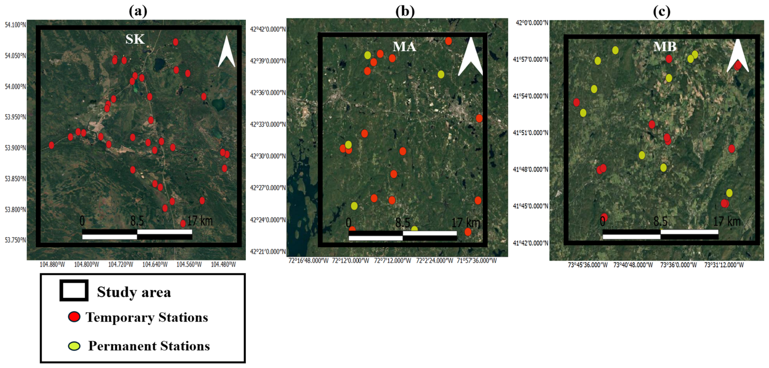
This study analyzes the Boreal Ecosystem Research and Monitoring Sites (BERMS), which are located in the southern section of the Boreal Plain Ecosystem (BPE) in central Saskatchewan (SK), Canada, together with the temperate and evergreen forests in Massachusetts and New York, United States. Figure 1 indicates the locations of the three forested areas. Each area includes a SM measurement network with approximately 20 to 37 stations distributed over approximately 25–40 km extents, encompassing the SMAP retrieval footprint at each location. The SM measurements were recorded during the SMAPVEX19-22 [51] and SMAPVEX-22-Boreal [58] campaigns.

BPE land consists of a mix of boreal forest types, which are predominantly composed of evergreen needle leaf (23%), deciduous broadleaf (19%), and mixed wood (5%) stands [58]. The main types of overstory trees on BPE land are trembling aspen, balsam poplar, paper or white birch, white spruce, black spruce, jack pine, and eastern larch or tamarack [59]. The boreal forest climate is classified as cool, sub-humid continental, characterized by an average annual precipitation of approximately 428 mm, which includes both rainfall and snowfall, and an average frost-free period lasting about 108 days [16].

The Massachusetts (MA) domain (42.34°N–42.69°N; 71.95°W–72.29°W), including the Harvard Forest, is dominated by the following land cover types: beech–maple forest (~46%), pine forest (~24%), oak–hickory forest (12%), wetlands (~13%), and ~4% grassland/hay fields. The operations for the domain were staged out of Amherst (MA), where the Microwave Remote Sensing Laboratory of the University of Massachusetts Amherst served as the logistical center for the campaign, with the storage for equipment and drying ovens for soil and vegetation samples.

The Millbrook (MB) domain in New York (41.68°N–42.03°N; 73.44°W–73.79°W) includes the Cary Institute of Ecosystem Studies, which served as the logistical centre during the campaign, with the storage for equipment and drying ovens for soil and vegetation samples. The deciduous forest in Millbrook is dominated by oak–hickory forests (~30%), beech–maple forests (~30%), and a few conifer forests composed of Hemlock, which make up about 4%. The remaining 36% is non-forested, of which 23% is identified as pasture or hay fields, according to the National Land Cover Database (NLCD) [16,43]. The temperate forests are classified as cool continental to warm temperate, characterized by hot, humid summers and mild to cool winters. Annual precipitation averages between 100 and 150 cm, distributed relatively evenly throughout the year [60]. The campaigns included extensive characterization of surface roughness and vegetation using conventional and novel approaches [61,62,63,64]. To characterize the climatic regime of the three sites using a globally consistent standard, the United Nations Environment Programme (UNEP) Aridity Index (AI = P/PET) was computed for each location using the Global Aridity Index v3 dataset [65]. All three sites fall within the Humid class of the UNEP classification (AI ≥ 0.65; [66]). The boreal forest, SK, had a mean AI of 0.713 (range: 0.685–0.755), Harvard Forest, MA, had a mean AI of 1.301 (range: 1.250–1.368), and Millbrook, NY, had a mean AI of 1.270 (range: 1.150–1.466).

Each of the three forests (boreal and temperate) exhibits unique characteristics.

Table 1. Study area characteristics.

Study Area	Forest Type	Land Cover	References
Saskatchewan (SK)	Boreal	Jack pine, Black spruce, Mixed wood	[58]
Millbrook (MB)	Temperate	Red Maple, Sugar Maple, Hemlock, Pignut Hickory, Beech	[51]
Massachusetts (MA)	Temperate	Pine, Red-maple, Red Oak, Hemlock, Yellow Birch, Grey Birch	[51]

shows the dominant land cover of each forested site.

2.2. Dataset

2.2.1. L-Band Passive Microwave Data

This study utilized passive microwave measurements from the SMOS and SMAP satellites for correlation analysis and SM estimation. Both satellites provide L-band TB measurements globally every 1 to 3 days [43]. For this study, SM, VWC, VOD, TB, and MPDI data for both 6 AM and 6 PM local time overpasses were obtained from the SMAP L3 radiometer (version 8) and SMOS L3 (version 331) products. MPDI is an index that is obtained from the horizontal (H) and vertical (V) polarizations of TB, as defined by Equation (1) [67].

$$\mathrm{MPDI}={\displaystyle \frac{{TB}_V-{TB}_H}{{TB}_V+{ TB}_H}}$$

(1)

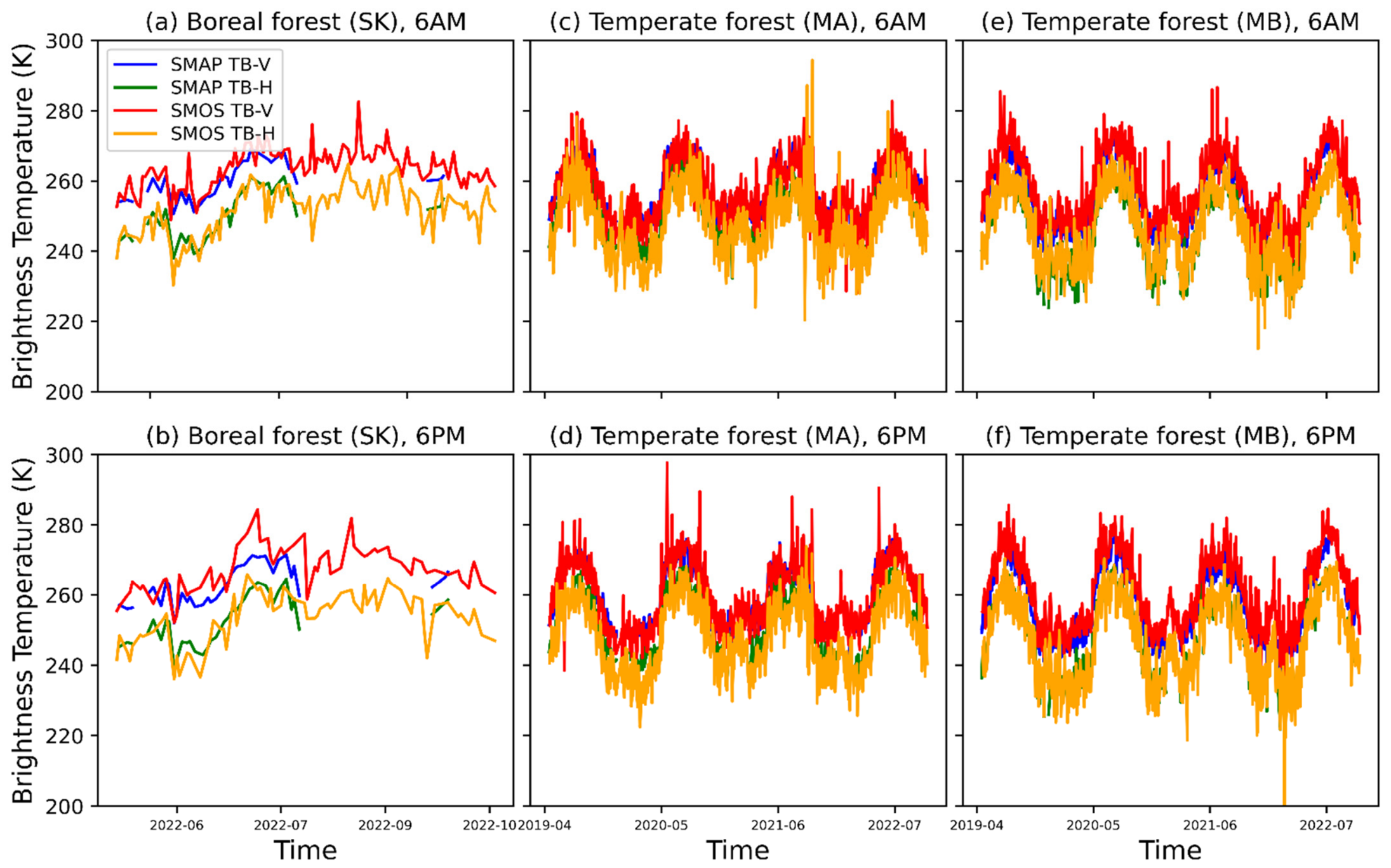
The grid resolutions of the SMAP and SMOS data are 36 km and 25 km, respectively. SMOS L3TB data are organized into 5-wide incidence angle bins and provides H and V polarizations. The SMAP L3 radiometer also provides TB in both H- and V-polarizations. Figure 2 illustrates the temporal variability in TB for H and V polarizations that are derived from SMAP and SMOS (40° incidence angle) for AM and PM overpasses across the three forest sites. The SMAP satellite experienced data outages from 20 June to 22 July 2019 and from 7 August to 25 September 2022, resulting in no available data during these periods [24,58]. SMOS L3SM uses several orbits to retrieve SM based on the L-band microwave emissions of the biosphere (L-MEB) radiative transfer model. The SMAP L3 SM products are based on DCA, using TB data in both H- and V-polarizations to retrieve SM. These L3 products provide improved SM retrievals by combining multiple observations, decreasing random noise, and providing structured results on daily or monthly timescales. Moreover, VOD was obtained from the SMAP L3 product, which is retrieved simultaneously with SM from dual-polarization TB using the regularized DCA based on RTM [68].

2.2.2. In Situ Dataset

SM, soil temperature, and air temperature were recorded hourly at the temporary and permanent stations located at the three forested sites. These ground measurements are used for correlation analyses, to evaluate the accuracy of SMAP and SMOS SM products, and to assess SM estimation methods developed in this study. The SM and temperature measurements in this study were taken at a depth of 0–5 cm, which is aligned with SMAP’s nominal retrieval depth [51,58]. This depth corresponds to probe placement within the organic forest-floor layer in the boreal stands [58]. In temperate forests, it represents a composite of the organic and upper mineral layers, depending on site-specific organic layer thickness. The temperate forest in Massachusetts contains more organic material in the top mineral layer (0–6 cm) than does the Millbrook site [51]. With respect to air temperature, measurements were taken at about 1.5 m height above the ground surface under the canopy in the MA and MB temperate forests [51] and at about 1 m height under the canopy in the boreal forest of SK as a proxy for canopy temperature.

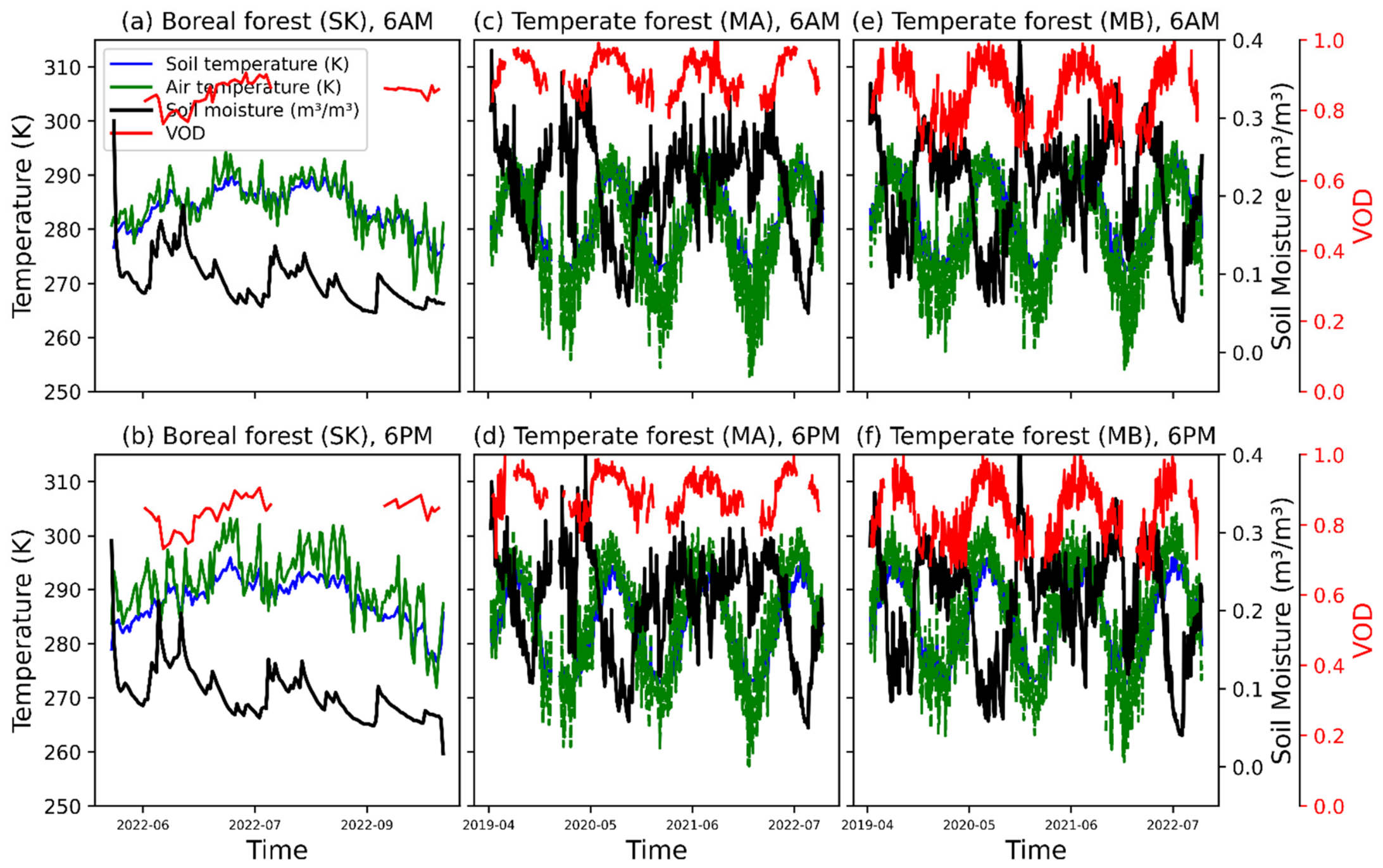
The dataset recorded for the three forested sites was available from 2019 to 2022 over the temperate forests and for 2022 over the boreal forest. Figure 1 illustrates the distribution of the temporary and permanent stations, and

Table 2. Distribution of temporary and permanent stations with their temporal coverage across three forest sites.

Site Characteristics	Boreal Forest	Temperate Forest (MA)	Temperate Forest (MB)
Number of Stations	37	25	25
Study Period	24 May 2022 to 19 October 2022	23 April 2019 to 15 November 2022	25 April 2019 to 17 November 2022

provides their temporal coverage across the three forest sites. In situ SM, air temperature, and soil temperature measurements were aligned with SMAP and SMOS satellite overpasses. Thus, for each forest site, morning (AM) and afternoon (PM) measurements correspond to the mean values of all available station records between 05:00 and 07:00 (AM) and 17:00 and 19:00 (PM), respectively. Figure 3 presents the time series of SM, air temperature, and soil temperature measurements from in situ stations, along with SMAP L3 VOD products at the three forest sites, for both AM and PM overpasses.

VWC was derived from climatology-based NDVI data representing vegetation greenness [69], which were obtained from daily MODIS observations [70]. According to

Table 3. Average air ($T_{air})$, soil temperatures ($T_{soil})$, and vegetation optical depth (VOD) during spring and summer for AM and PM periods, and average daily vegetation water content (VWC) during spring and summer across three forest sites.

Study Area	Year	Tair AM (K)	Tair PM (K)	Tsoil AM (K)	Tsoil PM (K)	VOD (AM)	VOD (PM)	VWC (kg/m2)
Boreal forest, SK	2022	285.60	292.37	285.0	288.87	0.84	0.82	12.52
Temperate forest, MA	2019	286.25	291.83	286.88	288.52	0.94	0.92	12.27
	2020	286.80	292.79	287.62	289.36	0.95	0.94	12.29
	2021	287.22	292.27	288.11	289.48	0.93	0.92	12.28
	2022	287.08	293.16	287.97	289.55	0.94	0.93	12.27
Temperate forest, MB	2019	287.39	293.55	288.50	290.59	0.91	0.89	10.81
	2020	287.63	294.68	288.78	290.91	0.92	0.91	10.87
	2021	287.96	293.90	289.13	290.75	0.91	0.89	10.87
	2022	287.86	295.22	289.14	291.20	0.91	0.89	10.85

, the three forest sites exhibited differences in air temperature ($T_{air}$), soil temperature ($T_{soil}$), VOD, and VWC. Differences in VWC and VOD can cause varying levels of attenuation of microwave radiation by vegetation at each forest site [51]. Moreover, air temperature exhibits greater variation between AM and PM than does soil temperature. It is therefore necessary to account for these variations in SM estimation for AM and PM overpasses.

2.3. Methodology

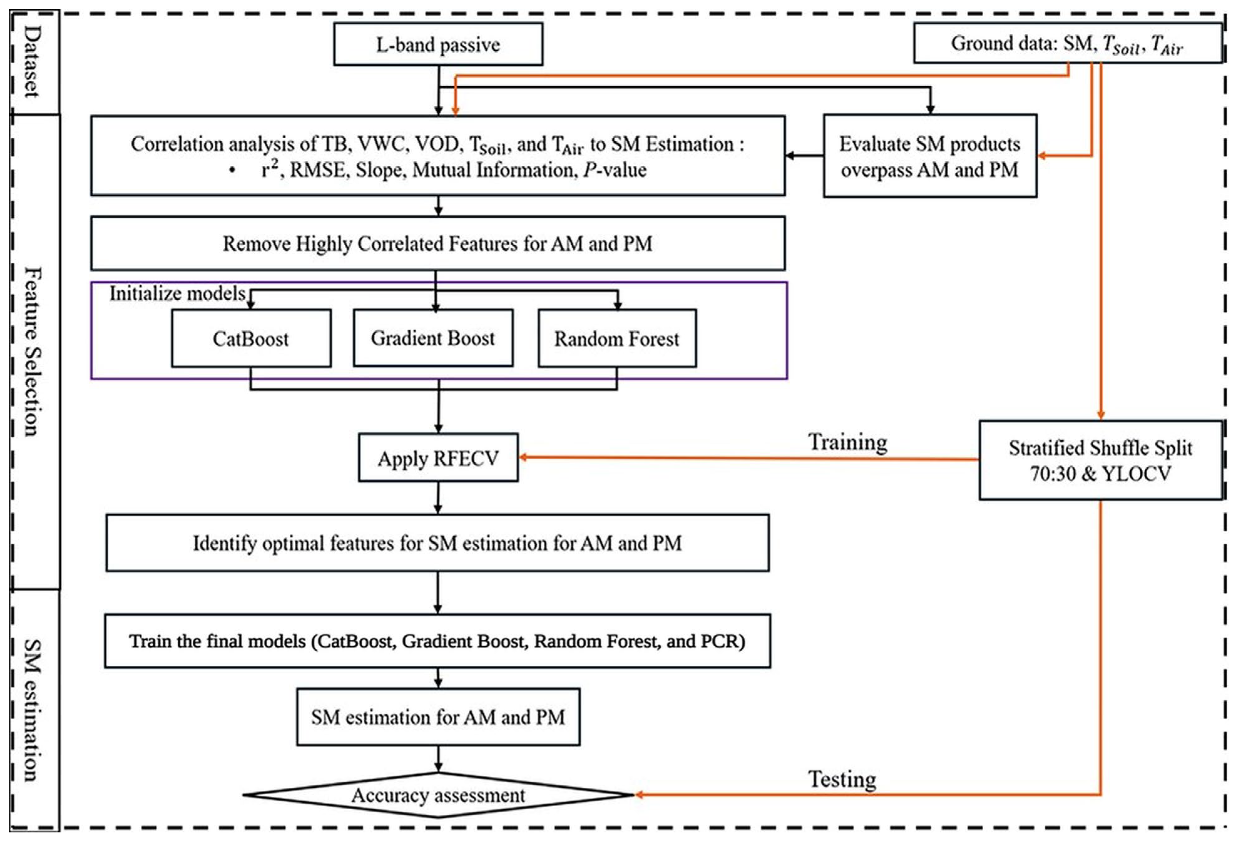
Snow and frozen conditions affect the quality and behavior of TB during the cold season [71]. Therefore, the study focused upon SM retrievals from TB measurements during the spring and summer periods (May to September). The proposed methodology for forest SM monitoring using ML is presented schematically in Figure 4. The study begins by evaluating the performance of SMAP and SMOS SM products through comparisons with in situ measurements in forested areas. The precision and reliability of these SM products were assessed using several statistical metrics, including the coefficient of determination (r²) calculated as the square of the Pearson correlation coefficient, RMSE, ubRMSE, and significance of the correlation coefficients (p-value) [37]. Moreover, correlation analysis was performed on datasets including SMAP and SMOS TB in H and V polarizations by evaluating their r² and p-value in relationship to their ground-based SM measurements to assess the potential of TB for SM estimation.

Different grid resolutions of SMAP and SMOS result in different spatial coverages, meaning that each sensor covers a different set of in situ stations within its grid cells, making their combined use less compatible for ML training. Moreover, SMOS provides TB at multiple incidence angles, and not all angles have observations available at each overpass, which limits the number of samples at a fixed angle (40°) for training an ML model. Beyond resolution and incidence-angle limitations, SMAP and SMOS data also use fundamentally different retrieval algorithms. SMAP L3 retrieves VOD through the DCA baseline using a single-angle dual-polarization tau–omega RTM, with VWC obtained from ancillary data derived from MODIS NDVI at 36 km resolution [68]. In contrast, SMOS retrieves VOD through a multi-angular L-MEB Bayesian inversion without an ancillary VWC product [48]. As the products from the two missions are produced by different physical models and depend on different ancillary information, they are not directly interchangeable. Therefore, combining them as ML features in the same input column could introduce systematic inconsistencies rather than additional information [72,73]. Moreover, downscaling and data-fusion methods for SMAP and SMOS SM retrievals typically operate on existing satellite SM products to disaggregate them to finer scales. However, when the underlying retrieval has limited accuracy over forests, these uncertainties may be propagated to the downscaled product [74]. For these reasons, SM estimation using ML was conducted with SMAP data only, as it provides a larger number of TB observations at a fixed incidence angle with greater temporal coverage over the study area, making these data more suitable for training ML models. Improving SM retrieval accuracy over forests by investigating the relative importance of vegetation, air temperature, and soil temperature during both AM and PM overpasses, as pursued in this study, can help future downscaling and fusion efforts. Excluding SMOS therefore does not artificially limit the model, as SMAP alone provides sufficient temporal coverage and observational consistency. The proposed framework can nonetheless be applied to SMOS separately once sufficient training data become available for ML model training. Feature selection was conducted on datasets including SMAP TB in H and V polarizations, VOD, MPDI, MODIS NDVI-derived VWC, and soil and air temperatures that were obtained from network measurements to identify the optimal features for SM estimation. Three ML models, i.e., CatBoost, GB, and RF, were trained to estimate SM for both AM and PM using two complementary training and evaluation strategies. In addition, PCR, as a linear model, was used under the same training strategies to provide a benchmark comparison with the non-linear models.

In the first strategy, a leave-one-year-out cross-validation (LOYOCV) scheme was applied to the MB and MA sites, where four-year ground SM data were available. The boreal forest site (SK) was excluded from this strategy due to the limited data availability, as SM measurements were only available for 2022. In the second strategy, the dataset was split into training (70%) and testing (30%) subsets using a stratified shuffle split (SSS) strategy [75,76,77,78].

2.3.1. Evaluation of SMAP and SMOS L3SM

To evaluate the accuracy of the SMAP and SMOS Level 3 SM products over forested areas, we compared them with ground-based SM measurements, focusing on both AM and PM overpasses. Ground measurements from all stations within each SMAP (36 km) and SMOS (25 km) pixels were averaged to match the grid resolutions of the respective satellite products. The precision and reliability of these SM products were assessed using statistical metrics, including r² (and the p-value), RMSE, and ubRMSE.

2.3.2. Correlation Analysis of SMAP and SMOS TB, MPDI, VOD vs. VWC, In Situ T_air and T_soil for SM Estimation

This correlation analysis of SMAP and SMOS TB, MPDI, VWC, air temperature, and soil temperature for SM estimation is conducted for the AM and PM overpasses. The r² (and the p-value), RMSE, slope, and mutual information, along with feature selection methods, including the removal of highly correlated features and recursive feature elimination with cross-validation (RFECV), were used in ML algorithms to identify key dependencies and limitations that influence SM retrieval accuracy in forests.

2.3.3. Feature Selection

This study employed a systematic feature selection methodology to identify optimal features for SM estimation across the three forest sites. By addressing issues such as multicollinearity and redundancy, we aimed to improve model accuracy and reduce computational complexity while deriving meaningful insights into the key factors influencing SM dynamics. Moreover, we evaluated the statistical significance of each feature for SM, with p-values that were derived from the t-distribution, where p < 0.05 indicated significant relationships between paired features and between features and SM.

The process of feature selection commenced by evaluating, in terms of SM information, six primary features that were measured during SMAP AM and PM satellite overpasses: SMAP TB in V and H polarizations, MPDI, air temperature, soil temperature, and VWC. While these variables have potential predictive power, interrelations between them pose risks of redundancy, which necessitates a robust feature selection procedure. Our feature selection method is based on two techniques for identifying optimal features:

(a)

A preliminary correlation analysis was conducted to identify and remove highly interdependent variables, thereby reducing multicollinearity and improving model interpretability. Pearson’s correlation coefficient was computed among all input features, and a fixed threshold of 0.8 was used to identify highly correlated feature pairs, indicating collinearity between predictors ([79,80]). For each correlated pair, the earlier-listed variable was retained, while the later-listed variable was removed, ensuring a deterministic and reproducible selection procedure. This filtering step was applied to the full dataset before cross-validation to keep the retained feature set consistent across both training schemes, including random splitting and LOYOCV. This filtering step was applied separately to AM and PM datasets, resulting in two refined feature sets: one for AM and one for PM observations.

(b)

To further refine the feature set, Recursive Feature Elimination with Cross-Validation (RFECV) was used. It iteratively removes the least significant features while validating model performance through cross-validation [81]. RFECV is a wrapper-based feature selection technique that leverages an ML algorithm to identify the most relevant features for model training [82]. This process resulted in an optimized set of features selected for SM estimation under varying temporal conditions.

In this research, feature selection was performed on the training set using RFECV, by applying a 5-fold cross-validation scheme with r² as the scoring metric to evaluate feature subsets. To create the training and testing sets, two strategies were employed as described in Section 2.3: (1) a LOYOCV applied exclusively to the MA and MB Forest sites, in which the model was trained on data from three years and tested on the held-out fourth year, rotating through all four years (2019–2022) to produce four folds. In the LOYOCV strategy, RFECV was performed separately within each outer LOYOCV fold using only the training years. The held-out test year was not used during feature selection or model training, ensuring that RFECV remained independent of the test data; and (2) an SSS technique based on site, ensuring balanced representation of the three forest sites across their temporal variability and maintaining forest type diversity in both splits [83].

2.3.4. Machine-Learning Models

We used ensemble-based ML algorithms, including RF, GB, and CatBoost to address the non-linearity and complexity of SM estimation. These models were selected for their ability to capture patterns from optimally selected features and SM; they also provided an opportunity to assess the potential of bagging (RF) and boosting (GB, CatBoost) methods for estimating SM. Moreover, PCR was implemented as a linear baseline model to quantify the performance gain provided by the non-linear methods.

CatBoost, which is derived from categorical and boosting, employs symmetric decision trees as its core learners. It constructs multiple base learners sequentially while keeping the training sample set unchanged, thereby improving noise resistance through ordered boosting. The final SM estimation is obtained by aggregating the interconnected weak learners using weighted regression.

GB is another ensemble ML method that sequentially incorporates weak learner models, refining predictions at each stage to improve accuracy [57].

RF constructs multiple independent Classification and Regression Tree (CART) units. These individual trees are randomly combined to form a forest. When presented with new data, each tree in the ensemble contributes to the final regression outcome through a voting or averaging process. Key advantages of RF include its ability to randomly select samples, thereby enhancing model robustness, and reducing the risk of overfitting [84].

Hyper-parameters are settings that are determined before training a model [85]. A preliminary sensitivity analysis indicated that different numbers of decision trees (1000, 500, 250, and 100) do not have a critical effect on the overall accuracy of the models. In this study, the optimal number of decision trees for CatBoost, GB, and RF was selected using a trial-and-error approach based on the validation dataset rather than the testing dataset. This procedure was applied under both training strategies: random splitting and LOYOCV. For LOYOCV, the validation split was created within the three training years of each fold, while the held-out test year remained independent. The four tested tree counts (100, 250, 500, and 1000) produced very similar validation accuracy for both AM and PM. Therefore, 1000 decision trees were selected based on the lowest RMSE and the highest r² between the estimated SM and ground-based SM measurements. Another reason is that 1000 trees represent the default setting in CatBoost; we selected the same number of trees for RF and GB models to ensure a fair comparison. Furthermore, boosting models (CatBoost and GB) use sequential decision trees; therefore, the number of trees is not primarily determined by the sample size, but is usually chosen through validation on test data [86,87]. The remaining model-specific hyperparameters were kept at their default library values to ensure a consistent and transparent comparison among the models. Specifically, CatBoost used a learning rate automatically selected by the algorithm, an L2 leaf regularization value of 3, and the RMSE loss function. Gradient Boosting used a learning rate of 0.1 and the squared-error loss function. RF used bootstrap sampling and the squared-error criterion for node splitting.

PCR combines Principal Component Analysis (PCA) with linear regression, where the standardized predictors are first transformed into orthogonal principal components to reduce multicollinearity among the input features, and a linear regression is then fitted on these components [80]. Since RFECV cannot be directly applied during PCR training, the features previously selected by RFECV in the ensemble models were used as input to PCR to ensure a consistent comparison among all models.

The effectiveness of ML algorithms also strongly depends upon the input data quality [88,89]. This study used all optimal features selected through the feature selection methods and ground measurements of SM (982 samples) across the three forest sites to train and test the three ensemble learning models and PCR (Section 2.3.2).

In the LOYOCV strategy, temporal generalization was assessed at Millbrook and Harvard Forest, while the boreal forest served as an extra test set. In this approach, all four models (CatBoost, GB, RF, and PCR) were iteratively trained on data from all years except one and tested on the held-out year, thereby evaluating the temporal generalization capability of the models. Within each LOYOCV fold, 10% of the training data were held out as a validation set. In one LOYOCV fold, the models were trained on the earlier years (2019, 2020, and 2021) and tested on the final year (2022), corresponding to the train-on-earlier-years/test-on-final-year setup suggested by the reviewer. The same logic was applied in the other folds, where each year was used in turn as an independent held-out test year. The boreal forest site, for which ground data were available for a single year only (2022), was used as an additional independent test set to further assess the spatial transferability of the trained models to an unseen forest ecosystem. This combination of strategies allows for a comprehensive evaluation of model performance in terms of both temporal robustness and cross-site generalization, similarly as in [90].

In the SSS strategy, each model was trained using 70% of the optimized feature set and the corresponding ground-based SM measurements and then evaluated on the remaining 30% of the dataset. Within the 70% training partition, 10% of the samples were held out as a validation set for hyperparameter tuning. SSS is a data-splitting technique that is commonly used in ML to create representative training and testing sets. Several studies have used this method for training and evaluating ML models based on remote sensing data [76,77,78,91]. In our study, the test set contains strictly unseen data (no leakage from the training set), and stratification ensures that these test samples still reflect the diversity of forest types. The dataset consisted of three forest sites that differed in SM ranges over time (see Figure 3). Furthermore, the temporal resolution of the input TB data is approximately 3–4 days, based on the SMAP revisit frequency. SSS was applied with a fixed random state to randomize the sample selection over time. All these aspects help reduce temporal correlation between the training and testing sets, thereby lowering the risk of overfitting and avoiding overly optimistic results in SM estimation using ML. In this strategy, cross-validation was applied only within recursive feature elimination (RFE) to identify the most important features. Notably, cross-validation was performed exclusively on the training data during feature selection and was not used for final accuracy assessment. Model performance was evaluated separately on the test set.

3. Results

3.1. Evaluation of Soil Moisture Products

The results for evaluating the performance of SMAP and SMOS SM products showed that the current SMAP and SMOS SM products have large uncertainties in forested areas.

Table 4. Coefficient of determination (r²), RMSE, and bias of SMAP soil moisture products (AM-PM) compared to in situ measurements. Significant correlations are observed for all sites (p < 0.05).

Forest Type	Measurement Time	r2	RMSE (m3/m3)	ubRMSE (m3/m3)	Bias (m3/m3)
Boreal Forest, SK	AM	0.62	0.28	0.06	+0.27
Boreal Forest, SK	PM	0.57	0.31	0.06	+0.30
Temperate Forest, MB	AM	0.51	0.20	0.05	+0.19
Temperate Forest, MB	PM	0.55	0.21	0.05	+0.21
Temperate Forest, MA	AM	0.20	0.23	0.07	+0.22
Temperate Forest, MA	PM	0.18	0.24	0.07	+0.23

and

Table 5. Coefficient of determination (r²), RMSE, and bias of SMOS soil moisture products (AM-PM) compared to in situ measurements. Significant correlations are observed for all sites (p < 0.05).

Forest Type	Measurement Time	r2	RMSE (m3/m3)	ubRMSE (m3/m3)	Bias (m3/m3)
Boreal Forest, SK	AM	0.04	0.19	0.13	+0.13
Boreal Forest, SK	PM	0.10	0.19	0.12	+0.14
Temperate Forest, MB	AM	0.24	0.13	0.09	+0.09
Temperate Forest, MB	PM	0.18	0.12	0.10	+0.06
Temperate Forest, MA	AM	0.06	0.15	0.13	+0.07
Temperate Forest, MA	PM	0.04	0.16	0.13	+0.09

show r², RMSE, and ubRMSE between in situ SM and SMAP and SMOS SM across the three forest sites. Significant correlations are observed for all three forest sites (p < 0.05). However, the comparisons exhibited high RMSE. The ubRMSE across the three forest sites ranges from 0.05 m³/m³ to 0.07 m³/m³ for the SMAP L3 SM product and from 0.09 m³/m³ to 0.13 m³/m³ for the SMOS L3 product. The r²-value for SMAP varied between 0.18 and 0.62 across the sites, with boreal forests showing the highest r² value (0.62 for AM and 0.57 for PM), but also high RMSE that ranged between 0.28 m³/m³ and 0.31 m³/m³). In contrast, SMOS correlations were consistently lower (r² < 0.25 for both AM and PM, with RMSE between 0.11 m³/m³ and 0.19 m³/m³). Furthermore, in this study, the evaluation of SM products over the boreal forest was limited to the spring and summer of one year (2022), whereas the observations for temperate forest sites covered around four years (spring and summer from 2019 to 2022). This difference in the number of samples may have also contributed to the variation in accuracy that was observed between the sites.

3.2. Correlation Analysis

3.2.1. SMAP and SMOS TB

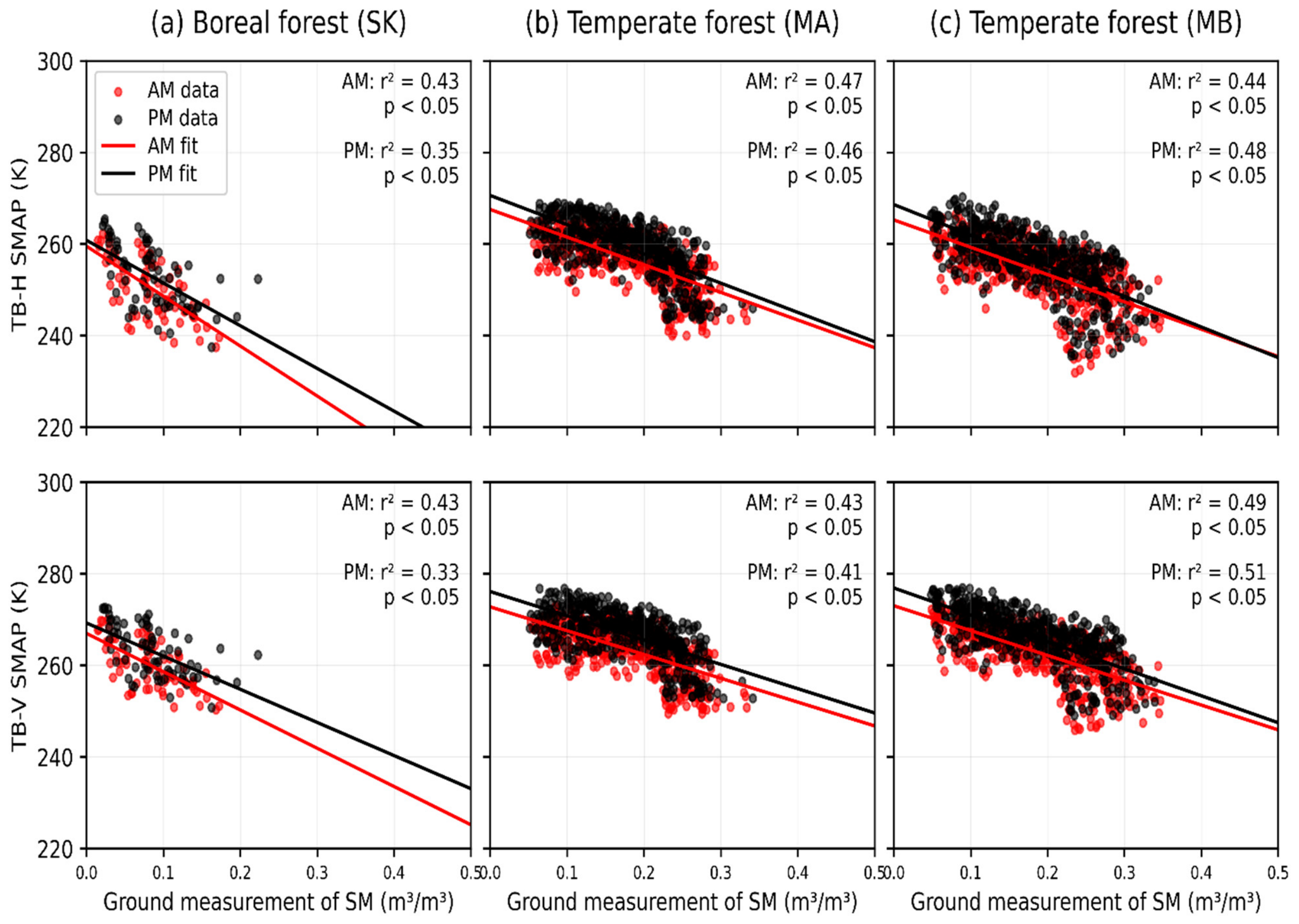
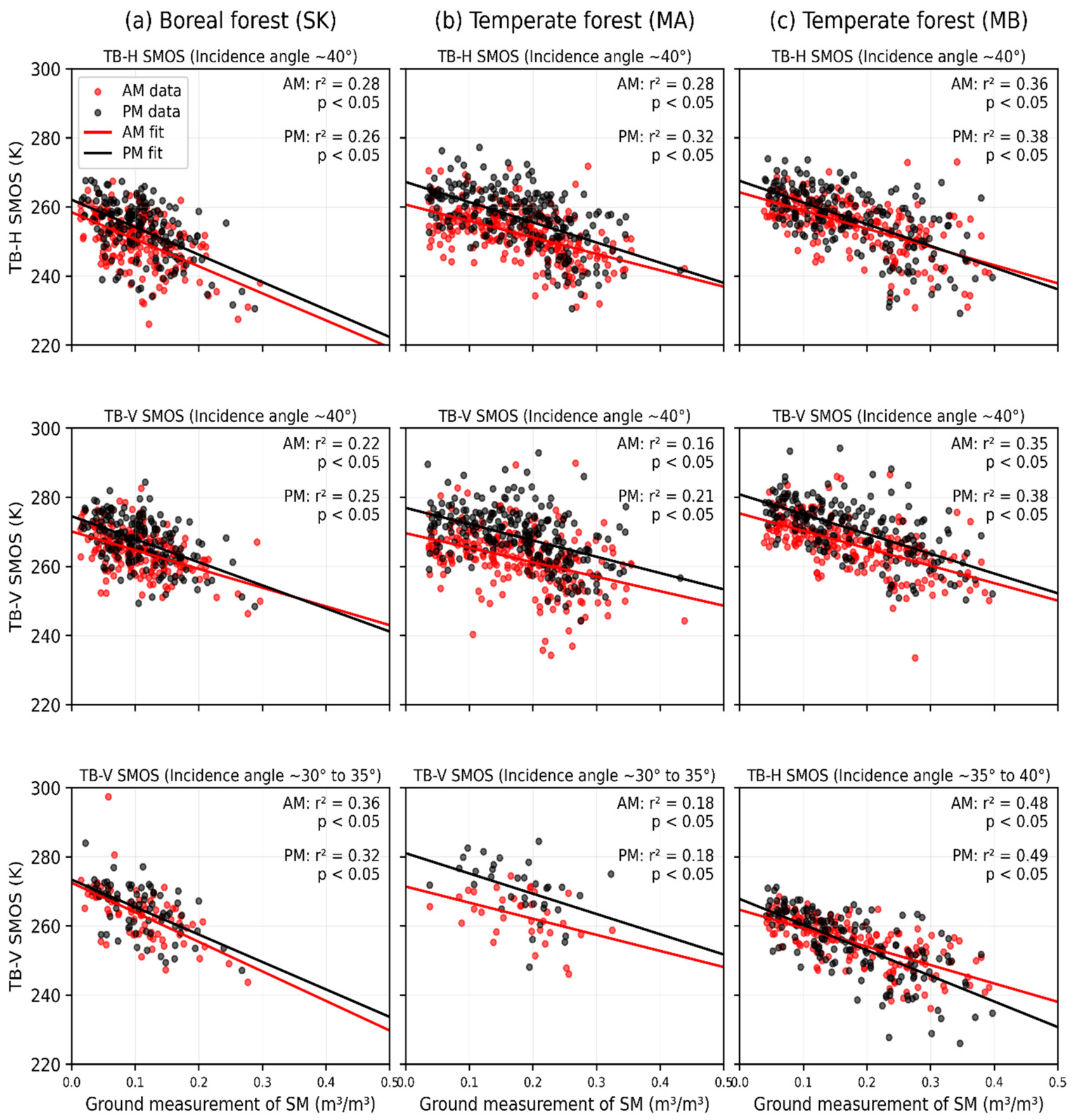
Figure 5 and Figure 6 show scatterplots of SM ground measurements and SMAP and SMOS TB across the three forest sites. Significant correlations were observed for all three forest sites (p < 0.05). Compared to the boreal forest, Figure 5 shows that higher SM, ranging from 0.05 to 0.35 m³/m³, is observed in the temperate forests during spring and summer, probably due to higher quantities or frequencies of precipitation (Section 2.1).

For SMAP TB in both V and H polarizations, r² values range from 0.33 to 0.51 for both AM and PM measurements across all sites, indicating a moderate relationship with the in situ SM. In contrast, SMOS TB (Figure 6) exhibits weaker correlations with in situ SM, where r² values range from 0.16 to 0.49 for both AM and PM measurements across the sites. The differences in correlations between SMAP and SMOS can be partly explained by the differences in the grid resolutions of the sensors. Indeed, SMAP has a grid spacing of 36 km while SMOS has 25 km, which affects the level of detail of the measurements and their agreement with ground-truth data.

3.2.2. Soil and Air Temperature

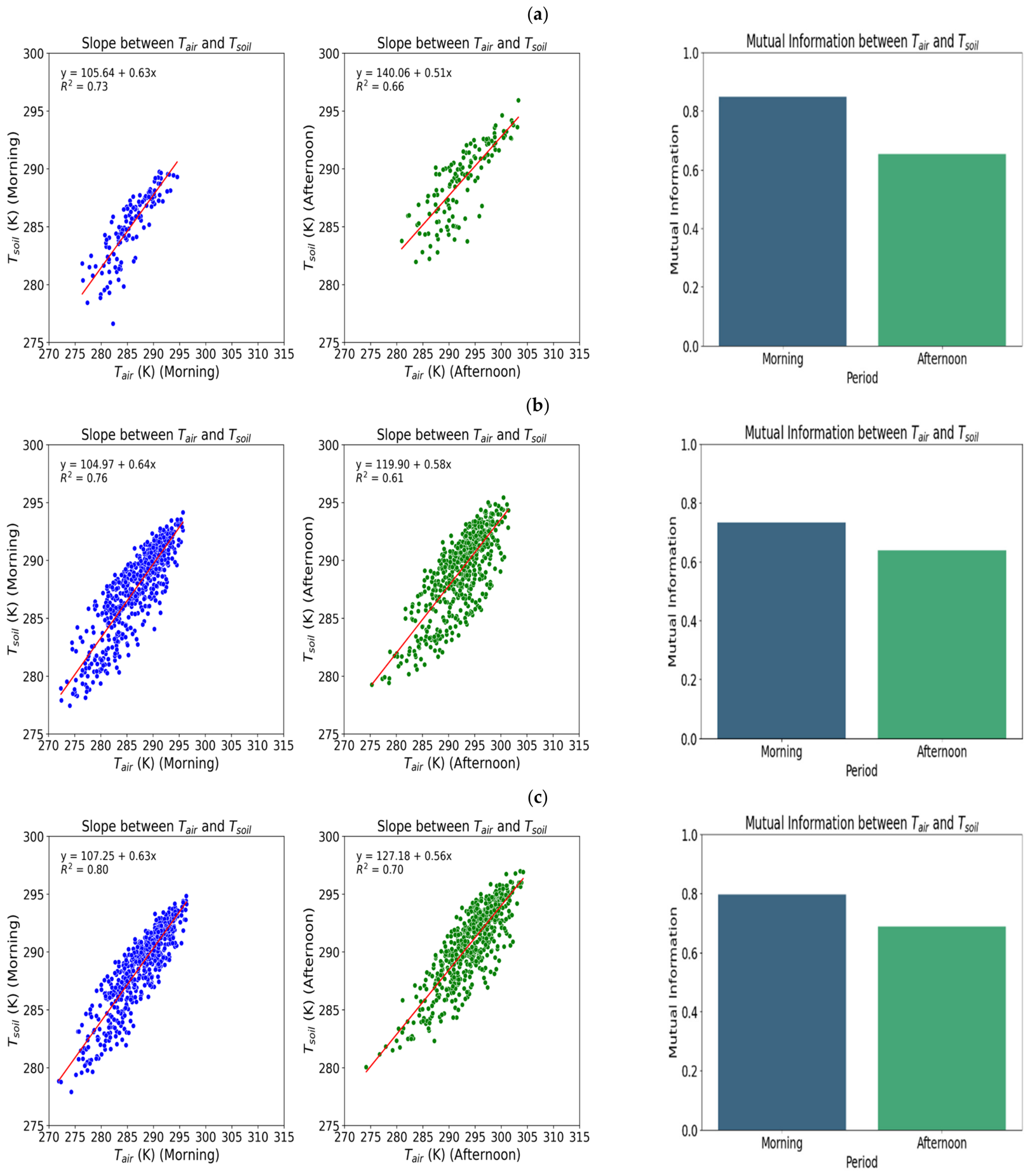
A detailed examination of mutual information and slope analyses across the three forest sites, as shown in Figure 7, reveals that r² between air and soil temperatures is consistently higher for the AM overpass time. During the PM overpass times, the slope and mutual information decrease, indicating distinct thermal variations between the dense canopy and soil (Figure 7).

The correlation analysis between air and soil temperatures highlights their importance in SM estimation for both AM and PM overpasses of SMAP and SMOS. This indicates that for the SMAP and SMOS PM overpasses, air and soil temperatures have distinct effects on SM estimation. The significant difference between air and soil temperatures observed in PM overpasses is primarily due to the thermal effect of the forest canopy.

3.3. Machine Learning

3.3.1. Feature Importance for Soil Moisture Estimation

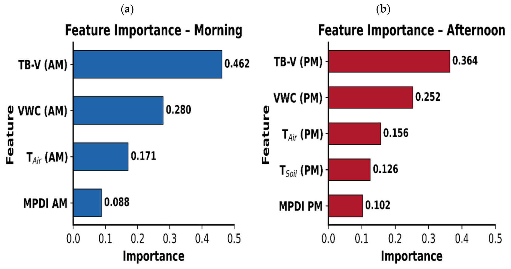
SM that was estimated using ML models depends on various input features, including TB-V, MPDI, soil and air temperature, and VWC. The relative importance of these features [92] was evaluated for both AM and PM timeframes using the built-in feature importance of the CatBoost model, which quantifies each feature’s contribution based on the average change in prediction values caused by splits on that feature across all trees in the ensemble. The results are shown in Figure 8.

The analysis shows that TB-V consistently exhibits the highest importance (~0.4) across all periods and timeframes. TB-H was removed through the feature selection process due to its strong correlation with TB-V, which made it redundant for improving model accuracy.

VWC was identified as the second most important feature (~0.25–0.28). It represents vegetation conditions associated with canopy greenness. Vegetation can absorb or scatter microwave emissions from the soil, thereby influencing the observed microwave signal. VOD, which represents the attenuation of microwave radiation by vegetation, was excluded during the feature selection process due to its high correlation with MPDI (r² ≈ 0.8) for both AM and PM overpasses. Although VOD captures important vegetation-related effects on microwave signals, its removal avoids feature redundancy in the model, as the combination of MPDI and VWC already retains the complementary vegetation information necessary for SM estimation. Temperature variables, although less significant than TB-V and VWC, provide valuable environmental input for SM estimation. The importance of air and soil temperature is more pronounced during PM overpasses, as they have distinct effects on SM. For AM overpasses, the model considers only air temperature, as air and soil temperatures exhibit similar trends (high value of mutual information, Figure 7). This was further confirmed through an additional experiment in which the accuracy of SM estimation was evaluated by varying temperature inputs using the CatBoost model. For AM, the model trained with air temperature alone achieved r² = 0.73 and RMSE = 0.04 m³/m³ and adding soil temperature produced negligible improvement (r² = 0.73, RMSE = 0.04 m³/m³), confirming that soil temperature does not contribute additional predictive information for AM retrieval. For PM, the model trained with air temperature alone achieved r² = 0.70 and RMSE = 0.04 m³/m³, and was improved by including both temperatures (r² = 0.74, RMSE = 0.04 m³/m³). Although MPDI ranks lower than other features, its consideration is essential for SM estimation in both AM and PM overpasses, as it helps mitigate the effects of NDVI saturation and improves the model’s ability to represent vegetation scattering, thereby reducing uncertainties associated with MODIS-derived VWC in forested areas. The study demonstrated the overall impact of these variables on SM estimation across forests for AM and PM, underscoring the importance of incorporating them into passive microwave SM retrieval algorithms. Moreover, in situ soil and air temperature measurements could be substituted with satellite-derived land surface temperature products such as MODIS LST or global climate reanalysis data, such as ERA5, for operational implementation where in situ data are not available.

3.3.2. Model Performance

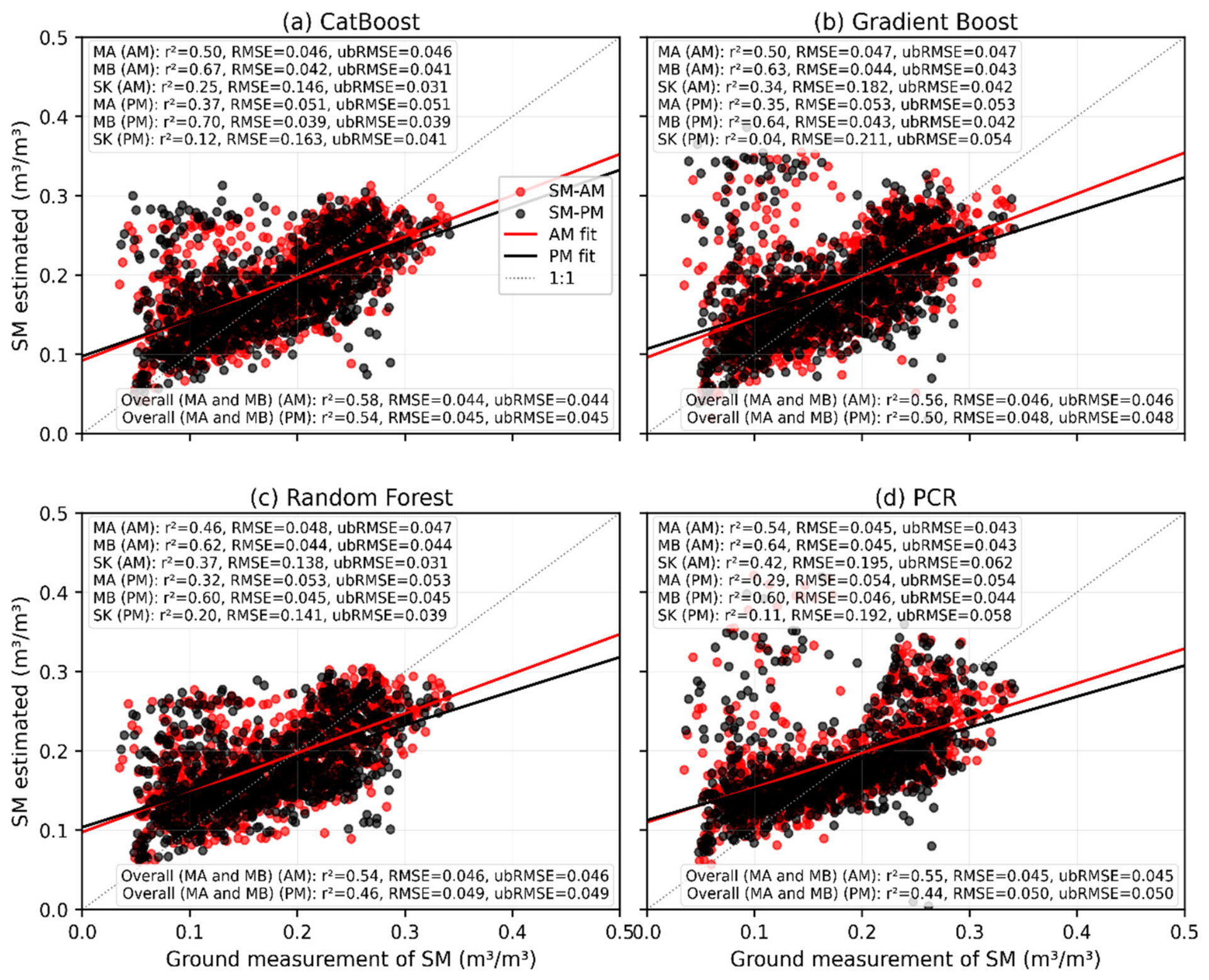
As illustrated in Figure 9, the LOYOCV strategy was applied to evaluate the temporal generalization of the models at MA and MB, while the boreal forest was used exclusively as an independent test set. The overall results at MA and MB showed that CatBoost achieved r² values of 0.58 (AM) and 0.54 (PM) with RMSE and ubRMSE values of 0.044 and 0.045 m³/m³, respectively. GB achieved r² values of 0.56 (AM) and 0.50 (PM) with RMSE and ubRMSE values of 0.046 and 0.048 m³/m³, and RF achieved r² values of 0.54 (AM) and 0.46 (PM) with RMSE and ubRMSE values of 0.046 and 0.049 m³/m³. PCR achieved r² values of 0.55 (AM) and 0.44 (PM), with RMSE and ubRMSE values of 0.045 and 0.050 m³/m³, respectively, showing lower accuracy than CatBoost and GB, particularly for PM. MB consistently outperformed MA across all models, with CatBoost recording r² values of 0.67 (AM) and 0.70 (PM) at MB compared to 0.50 (AM) and 0.37 (PM) at MA. The boreal forest showed poor accuracy (AM: r² = 0.25–0.42, RMSE = 0.138–0.195 m³/m³, ubRMSE = 0.031–0.062 m³/m³; PM: r² = 0.11–0.20, RMSE = 0.141–0.211 m³/m³, ubRMSE = 0.039–0.058 m³/m³). This lower accuracy compared to the other sites can be attributed to the limited number of available ground measurements at the boreal site, which were restricted to a single year (2022), preventing its inclusion in the training process. As a result, the models were unable to learn the unique characteristics of the boreal forest (e.g., vegetation density, canopy structure, and temperature) during training.

Table 6. Soil moisture estimation accuracy from the three machine-learning models (CatBoost, GB, RF) using the LOYOCV training strategy.

		AM				PM
Forest Sites	Model	r2	RMSE (m3/m3)	ubRMSE (m3/m3)	Bias (m3/m3)	r2	RMSE (m3/m3)	ubRMSE (m3/m3)	Bias (m3/m3)
SK	CatBoost	0.25	0.146	0.031	+0.14	0.12	0.163	0.041	+0.15
	GB	0.34	0.182	0.042	+0.18	0.04	0.211	0.054	+0.20
	RF	0.37	0.138	0.031	+0.13	0.20	0.141	0.039	+0.13
	PCR	0.42	0.195	0.062	+0.19	0.11	0.192	0.058	+0.18
MA	CatBoost	0.50	0.046	0.046	+0.01	0.37	0.051	0.051	0.00
	GB	0.50	0.047	0.047	+0.01	0.35	0.053	0.053	0.00
	RF	0.46	0.048	0.047	+0.01	0.32	0.053	0.053	0.00
	PCR	0.54	0.045	0.043	+0.01	0.29	0.054	0.054	0.00
MB	CatBoost	0.67	0.042	0.041	−0.01	0.70	0.039	0.039	0.00
	GB	0.63	0.044	0.043	0.00	0.64	0.043	0.042	0.00
	RF	0.62	0.044	0.044	0.00	0.60	0.045	0.045	0.00
	PCR	0.64	0.045	0.043	−0.01	0.60	0.046	0.044	−0.01
All Sites	CatBoost	0.58	0.044	0.044	0.00	0.54	0.045	0.045	0.00
	GB	0.56	0.046	0.046	0.00	0.50	0.048	0.048	0.00
	RF	0.54	0.046	0.046	0.00	0.46	0.049	0.049	0.00
	PCR	0.55	0.045	0.045	0.00	0.44	0.050	0.050	0.00

presents the accuracy of three ensemble models and PCR for estimating SM using the LOYOCV strategy for AM and PM overpasses across all forest sites, expressed in terms of r², RMSE, and ubRMSE.

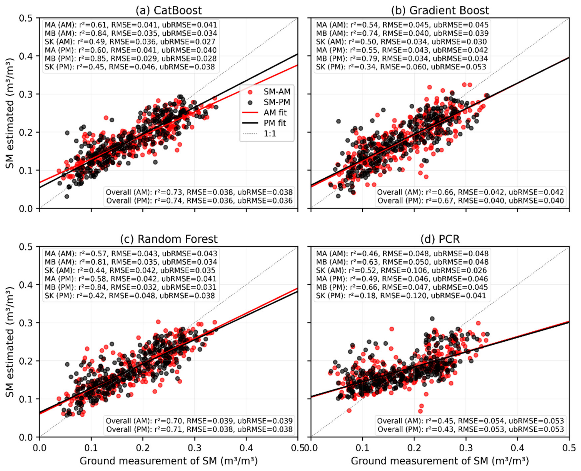
As illustrated in Figure 10, CatBoost, GB, and RF exhibited strong performance in estimating SM using the SSS strategy, with CatBoost leading slightly in terms of accuracy. These results were obtained using the testing dataset (30% of the total data) across three forest sites. CatBoost achieved the highest overall r² values of 0.73 (AM) and 0.74 (PM), paired with low respective RMSE and ubRMSE values of 0.038 m³/m³ (AM) and 0.036 m³/m³ (PM), which reflects its superior predictive capability. RF followed closely, with overall r² values of 0.70 (AM) and 0.71 (PM). Similarly, GB achieved close accuracy, with overall r² values of 0.66 (AM) and 0.67 (PM) and RMSE and ubRMSE values of 0.042 m³/m³ (AM) and 0.040 m³/m³ (PM), respectively. PCR achieved overall r² values of 0.45 (AM) and 0.43 (PM), with RMSE values of 0.054 and 0.053 m³/m³ and ubRMSE values of 0.053 and 0.053 m³/m³, respectively. Its lower performance compared to the non-linear ensemble models confirms the advantage of non-linear approaches over the linear baseline under the SSS strategy.

By focusing on each forest site (SK, MA, and MB), CatBoost recorded r² values of 0.49 (AM) and 0.45 (PM) for SK, 0.61 (AM) and 0.60 (PM) for MA, and 0.84 (AM) and 0.85 (PM) for MB. GB achieved r² values of 0.50 (AM) and 0.34 (PM) in SK, 0.54 (AM) and 0.55 (PM) in MA, and 0.74 (AM) and 0.79 (PM) in MB. RF demonstrated r² values of 0.44 (AM) and 0.42 (PM) in SK, 0.57 (AM) and 0.58 (PM) in MA, and 0.81 (AM) and 0.84 (PM) in MB. PCR yielded r² values of 0.52 (AM) and 0.18 (PM) in SK, 0.46 (AM) and 0.49 (PM) in MA, and 0.63 (AM) and 0.66 (PM) in MB. Across all forest sites, RMSE and ubRMSE values that emerged from the four models ranged between 0.036 m³/m³ and 0.054 m³/m³.

Table 7. Soil moisture estimation accuracy from the three machine-learning models (CatBoost, GB, RF) using the SSS training strategy.

		AM				PM
Forest Sites	Model	r2	RMSE (m3/m3)	ubRMSE (m3/m3)	Bias (m3/m3)	r2	RMSE (m3/m3)	ubRMSE (m3/m3)	Bias (m3/m3)
SK	CatBoost	0.49	0.036	0.027	+0.02	0.45	0.046	0.038	+0.03
	GB	0.50	0.034	0.030	+0.02	0.34	0.060	0.053	+0.03
	RF	0.44	0.042	0.035	+0.02	0.42	0.048	0.038	+0.03
	PCR	0.52	0.106	0.026	+0.10	0.18	0.120	0.041	+0.11
MA	CatBoost	0.61	0.041	0.041	0.00	0.60	0.041	0.040	+0.01
	GB	0.54	0.045	0.045	0.00	0.55	0.043	0.042	+0.01
	RF	0.57	0.043	0.043	0.00	0.58	0.042	0.041	0.00
	PCR	0.46	0.048	0.048	−0.01	0.49	0.046	0.046	0.00
MB	CatBoost	0.84	0.035	0.034	−0.01	0.85	0.029	0.028	0.00
	GB	0.74	0.040	0.039	−0.01	0.79	0.034	0.034	−0.01
	RF	0.81	0.035	0.034	−0.01	0.84	0.032	0.031	−0.01
	PCR	0.63	0.050	0.048	−0.01	0.66	0.047	0.045	−0.01
All Sites	CatBoost	0.73	0.038	0.038	0.00	0.74	0.036	0.036	0.00
	GB	0.66	0.042	0.042	0.00	0.67	0.040	0.040	0.00
	RF	0.70	0.039	0.039	0.00	0.71	0.038	0.038	0.00
	PCR	0.45	0.054	0.053	0.00	0.43	0.053	0.053	0.00

presents the accuracy of the three ensemble models and PCR for estimating SM using the SSS strategy for AM and PM overpasses across all forest sites.

4. Discussion

The SMAP and SMOS SM products showed limited accuracy over forested regions, which is consistent with previous studies. Berg et al. [58] evaluated the accuracy of SMAP L2-enhanced SM products and SMOS L2 products against ground-based measurements in the organic soil layer of the boreal forest. The SMAP products that were based on the DCA demonstrated stronger correlations with in situ observations (r = 0.54 for AM, 0.57 for PM) and a ubRMSE of 0.06 m³/m³. In contrast, SMOS products showed weaker correlations (r = 0.40 for AM, 0.46 for PM) and higher ubRMSE values (0.10 m³/m³ for AM, 0.07 m³/m³ for PM). Although SMAP SM products exhibited better performance, they showed a more pronounced wet bias, as indicated by higher RMSE values than SMOS SM products [58], which is consistent with our findings. Moreover, a study by Ambadan et al. [16] analyzed the accuracy of SMAP L2 SM products based on the Tau–Omega SCA. They found a low r (<0.4) over boreal forests. Park et al. [23] retrieved SM from SMAP TB data using MPDI that was adjusted within the τ–ω model under forests, achieving r of 0.44 and an ubRMSE of 0.125 m³/m³. Overall, the results indicate that existing SMAP and SMOS SM products exhibit limited accuracy in densely vegetated regions due to attenuation and scattering effects incurred by the forest canopy. This limitation likely occurs, given that beyond a certain level of VWC, vegetation attenuation and scattering of surface emissions become too strong to allow accurate SM estimation. Previous studies have demonstrated that these SM products perform better in environments with lower vegetation density, typically where VWC does not exceed 5 kg/m² [23,43,93]. However, based on MODIS NDVI-derived VWC data, Table 3 shows that our forest sites exhibit considerably higher VWC, ranging from 10.81 kg/m² to 12.52 kg/m², affecting the SM retrieval accuracy.

SMAP and SMOS TB showed moderate correlations with SM, with r² values ranging from 0.16 to 0.49. Ambadan et al. [16] showed correlations between SMAP TB and mineral layer SM of about −0.65 for H-polarization and −0.6 for V-polarization over the boreal forest site. Overall, SMAP TB is valuable for SM estimation in forested areas. These studies support its sensitivity to SM under forest canopies. Yet, existing retrieval algorithms assume greater signal attenuation than what is observed from L-band passive microwave observations [43]. This highlights the need to consider vegetation properties, including attenuation and scattering parameters, together with surface temperature, for accurate SM estimation under forest canopies [23,24,49].

Furthermore, mutual information and slope analyses showed that the relationship between soil and air temperatures was stronger during AM overpasses than during PM overpasses, indicating a closer thermal coupling in the morning and distinct thermal behaviour between the canopy and the soil in the afternoon. This contrast can be explained by canopy–soil energy exchange. Dense vegetation reduces solar radiation reaching the ground through canopy shading, limiting daytime soil heating. As a result, the soil cools faster in the afternoon, while the canopy retains absorbed energy and releases it gradually, causing the air within it to cool more slowly than the soil [94]. This differential cooling alters the air–soil temperature relationship and consequently affects SM retrieval. This finding agrees with Abdelkader et al. [49], who compared SMAP Level 2 SM retrievals with in situ data in forests and found better accuracy in the morning (Mean Differences (MD) of 0.09–0.17 m³/m³) than in the afternoon (MD of 0.12–0.20 m³/m³), which is likely due to the assumption in the SM retrieval algorithm that air temperature is considered equivalent to soil temperature for both AM and PM overpasses [49].

Subsequently, feature importance analysis derived from the CatBoost model identified TB as the most influential variable for SM estimation during both AM and PM overpasses, followed by VWC, air temperature, and MPDI during AM overpasses, and by VWC, air temperature, soil temperature, and MPDI during PM overpasses. The inclusion of soil temperature as an additional predictor in the PM model reflects its distinct effect relative to air temperature during afternoon overpasses, as indicated by the mutual information analysis discussed above. TB in both H and V polarizations, derived from SMAP, is sensitive to changes in the soil’s dielectric constant, reflecting variations in SM [95,96]. The importance of TB-V is slightly higher in the morning (~0.46) compared to the afternoon (~0.36). This is likely because the temperature difference between the canopy and soil is smaller during the AM overpasses than the PM overpasses, reducing the impact of soil temperature on TB for SM estimation [24]. Previous studies have also indicated that surface temperature effects are more pronounced during PM overpasses compared to AM overpasses, impacting the TB of the soil [97]. Model performance underscores the critical role of TB-V as a fundamental component in SM estimation models.

The results of SM estimation from the ML models the SSS strategy is preferable to the LOYOCV method because it allows the models to learn the characteristics of both boreal and temperate forest sites simultaneously, thereby improving SM estimation accuracy. Furthermore, Differences in accuracy across the forest sites, as indicated by r², RMSE and ubRMSE, can be attributed to site-specific characteristics (Table 3). This aligns with the findings of Colliander et al. [24], who had retrieved SM using a parameterized emission model. Their retrievals that were based on TB-V polarization achieved higher accuracy in the MB (r = 0.82–0.85; ubRMSD = 0.049–0.050; p < 0.01) than in MA (r = 0.66–0.75; ubRMSD = 0.048–0.053; p < 0.01). Furthermore, in contrast to the retrieval accuracy that was obtained for SMAP SM products (Table 4), SM retrieval accuracy resulting from these ML algorithms is in accord with the quantity of biomass. The ML-based SM estimation achieved notably higher accuracy than the SMAP products, especially at the MA and MB sites, using both SSS and LOYOCV training methods. The low performance at the boreal forest site is likely due to the limited number of available training samples. These results highlight that while all ML models provide robust SM predictions, CatBoost remains the most accurate model, followed closely by GB and RF.

The proposed framework was developed and evaluated across three forested sites, all of which fall within the Humid class of the UNEP Aridity Index (AI ≥ 0.65) (Section 2.1). Although all sites belong to the same broad climate class, they represent a meaningful range of vegetation densities and canopy structures within humid forests, providing a robust baseline for evaluating L-band passive microwave soil moisture retrieval in this ecosystem class. The sites were selected because they correspond to the NASA SMAP Validation Experiment campaigns (SMAPVEX19–22 [51] and SMAPVEX22-Boreal [58]), which provide ground SM measurements under forest canopies. These datasets directly address one of the long-standing challenges in low-frequency microwave remote sensing, namely the retrieval of soil moisture in forests, where SMAP and SMOS products have historically shown high uncertainty due to limited ground validation measurements [51]. Future work should extend the framework to additional climate regimes, including sub-humid, semi-arid, and arid forests, to evaluate the effects of vegetation, soil temperature, and air temperature on SM estimation from L-band TB during both AM and PM overpasses. Such an extension would also enable a Spearman correlation analysis between model performance and the AI gradient, together with the evaluation of adaptive dynamic merging across different climate classes. Furthermore, the present study estimates SSM at the nominal L-band microwave sensing depth of 0–5 cm, consistent with the physical penetration depth of the 1.4 GHz signal into the soil column [35,36] and with the validation depth adopted for SMAP and SMOS products [98]. The ground reference networks used in this study were instrumented at the same depth, ensuring physical consistency between the L-band TB observations and ground-based SM measurements. SSM plays an important role in ecosystem carbon balance; however, carbon sequestration is a complex process influenced by many interacting factors [3]. In forest ecosystems, processes such as water stress, transpiration, and carbon–water coupling are governed not only by SSM but also by root-zone soil moisture (RZSM, 0–100 cm) [99]. However, RZSM cannot be directly retrieved from L-band radiometry because of its limited penetration depth [44,100]. Therefore, an established pathway for future studies to propagate L-band surface observations to the root zone is to assimilate SM estimations into a land surface model using data assimilation techniques [100,101].

5. Conclusions

We developed an ML method trained using combined boreal and temperate forest data to estimate SM in both forest types. The proposed method estimates SM using L-band passive microwave data and investigates the effect of air temperature, soil temperature, MPDI, VOD, and VWC on SM estimation during AM and PM satellite overpasses. This study conducted a comprehensive analysis of SM estimation across three forest sites, (1) to evaluate the accuracy of SMAP and SMOS SM products, (2) to conduct correlation analysis and feature selection to identify key features for SM estimation during both AM and PM satellite overpasses, and (3) to estimate SM during both AM and PM overpasses using CatBoost, GB, RF, and PCR models.

The results indicate that current SMAP and SMOS SM products suffer from great uncertainties in dense forests. Compared to the retrieval accuracy of SMAP and SMOS SM products, the three ML algorithms yield more accurate SM retrievals. The ML algorithms use soil temperature, air temperature, MPDI, VOD, and VWC during both AM and PM overpasses.

A key contribution of this study is that it underscores the role of air and soil temperatures, MPDI, and VWC in SM estimation for both AM and PM overpasses based on correlation analysis and feature importance analysis. Correlation analysis reveals a strong association between air and soil temperatures during SMAP and SMOS AM overpasses, allowing them to be used interchangeably for SM estimation. However, this relationship changes during PM overpasses, given that air and soil temperatures exhibit distinct effects on SM estimation. This variation is likely due to the thermal absorption effect of dense vegetation, preventing canopy cooling relative to that of the soil.

Feature importance analysis confirmed that TB-V consistently exhibits the highest importance due to its sensitivity to changes in the soil’s dielectric constant, followed by VWC, air and soil temperatures, and MPDI. VWC modulates microwave signals by either absorbing or scattering emissions from the soil surface. However, no significant difference in VWC effects was observed between AM and PM overpasses, which may be explained by the fact that daily VWC was derived from climatology-based MODIS NDVI. A more precise dataset would be beneficial for better assessing the influence of VWC across different timeframes. Among the ML models, the ensemble methods (CatBoost, GB, and RF) showed close performance in SM estimation and outperformed PCR under the SSS training strategy. Overall, CatBoost showed slightly higher accuracy. However, model performance varied by site and overpass time, with RF and GB outperforming CatBoost at some sites. These findings emphasize the critical role of L-band TB and the significant impact of VWC, MPDI, soil and air temperatures on SM estimation over forests, for both AM and PM overpasses.

References

1. Wadsworth, E.; Champagne, C.; Berg, A.A. Evaluating the Utility of Remotely Sensed Soil Moisture for the Characterization of Runoff Response over Canadian Watersheds. Can. Water Resour. J. Rev. Can. Ressour. Hydr. 2020, 45, 77–89. [Google Scholar] [CrossRef]
2. Purdy, A.J.; Fisher, J.B.; Goulden, M.L.; Colliander, A.; Halverson, G.; Tu, K.; Famiglietti, J.S. SMAP Soil Moisture Improves Global Evapotranspiration. Remote Sens. Environ. 2018, 219, 1–14. [Google Scholar] [CrossRef]
3. Falloon, P.; Jones, C.D.; Ades, M.; Paul, K. Direct Soil Moisture Controls of Future Global Soil Carbon Changes: An Important Source of Uncertainty. Glob. Biogeochem. Cycles 2011, 25, GB3010. [Google Scholar] [CrossRef]
4. Larson, J.; Wallerman, J.; Peichl, M.; Laudon, H. Soil Moisture Controls the Partitioning of Carbon Stocks across a Managed Boreal Forest Landscape. Sci. Rep. 2023, 13, 14909. [Google Scholar] [CrossRef]
5. Kemppinen, J.; Niittynen, P.; Rissanen, T.; Tyystjärvi, V.; Aalto, J.; Luoto, M. Soil Moisture Variations from Boreal Forests to the Tundra. Water Resour. Res. 2023, 59, e2022WR032719. [Google Scholar] [CrossRef]
6. Thomas Ambadan, J.; Oja, M.; Gedalof, Z.; Berg, A.A. Satellite-Observed Soil Moisture as an Indicator of Wildfire Risk. Remote Sens. 2020, 12, 1543. [Google Scholar] [CrossRef]
7. van Wagner, C. Development and Structure of the Canadian Forest Fire Weather Index System; Canadian Forestry Service: Ottawa, ON, Canada, 1987; ISBN 0-662-15198-4. [Google Scholar]
8. Rodriguez-Jimenez, F.; Lorenzo, H.; Novo, A.; Acuna-Alonso, C.; Alvarez, X. Modelling of Live Fuel Moisture Content in Different Vegetation Scenarios during Dry Periods Using Meteorological Data and Spectral Indices. For. Ecol. Manag. 2023, 546, 121378. [Google Scholar] [CrossRef]
9. Peng, J.; Albergel, C.; Balenzano, A.; Brocca, L.; Cartus, O.; Cosh, M.H.; Crow, W.T.; Dabrowska-Zielinska, K.; Dadson, S.; Davidson, M.W. A Roadmap for High-Resolution Satellite Soil Moisture Applications–Confronting Product Characteristics with User Requirements. Remote Sens. Environ. 2021, 252, 112162. [Google Scholar] [CrossRef]
10. Judge, J.; Liu, P.-W.; Monsiváis-Huertero, A.; Bongiovanni, T.; Chakrabarti, S.; Steele-Dunne, S.C.; Preston, D.; Allen, S.; Bermejo, J.P.; Rush, P. Impact of Vegetation Water Content Information on Soil Moisture Retrievals in Agricultural Regions: An Analysis Based on the SMAPVEX16-MicroWEX Dataset. Remote Sens. Environ. 2021, 265, 112623. [Google Scholar] [CrossRef]
11. Wang, T.; Zhang, H.; Zhao, J.; Wu, R.; Li, H.; Guo, X.; Zhao, H. Increased Atmospheric Moisture Demand Induced a Reduction in the Water Content of Boreal Forest during the Past Three Decades. Agric. For. Meteorol. 2023, 342, 109759. [Google Scholar] [CrossRef]
12. Bourgeau-Chavez, L.L.; Garwood, G.; Riordan, K.; Cella, B.; Alden, S.; Kwart, M.; Murphy, K. Improving the Prediction of Wildfire Potential in Boreal Alaska with Satellite Imaging Radar. Polar Rec. 2007, 43, 321–330. [Google Scholar] [CrossRef]
13. Lavoie, M.; Paré, D.; Fenton, N.; Groot, A.; Taylor, K. Paludification and Management of Forested Peatlands in Canada: A Literature Review. Environ. Rev. 2005, 13, 21–50. [Google Scholar] [CrossRef]
14. Simon, B.; Crowley, C.; Franco, F. The Costs and Costs Avoided from Wildfire Fire Management—A Conceptual Framework for a Value of Information Analysis. Front. Environ. Sci. 2022, 10, 804958. [Google Scholar] [CrossRef]
15. Bircher, S.; Andreasen, M.; Vuollet, J.; Vehviläinen, J.; Rautiainen, K.; Jonard, F.; Weihermüller, L.; Zakharova, E.; Wigneron, J.-P.; Kerr, Y.H. Soil Moisture Sensor Calibration for Organic Soil Surface Layers. Geosci. Instrum. Methods Data Syst. 2016, 5, 109–125. [Google Scholar] [CrossRef]
16. Ambadan, J.T.; MacRae, H.C.; Colliander, A.; Tetlock, E.; Helgason, W.; Gedalof, Z.; Berg, A.A. Evaluation of SMAP Soil Moisture Retrieval Accuracy over a Boreal Forest Region. IEEE Trans. Geosci. Remote Sens. 2022, 60, 4414611. [Google Scholar] [CrossRef]
17. Vereecken, H.; Huisman, J.A.; Pachepsky, Y.; Montzka, C.; van der Kruk, J.; Bogena, H.; Weihermüller, L.; Herbst, M.; Martinez, G.; Vanderborght, J. On the Spatio-Temporal Dynamics of Soil Moisture at the Field Scale. J. Hydrol. 2014, 516, 76–96. [Google Scholar] [CrossRef]
18. Coopersmith, E.J.; Cosh, M.H.; Petersen, W.A.; Prueger, J.; Niemeier, J.J. Soil Moisture Model Calibration and Validation: An ARS Watershed on the South Fork Iowa River. J. Hydrometeor. 2015, 16, 1087–1101. [Google Scholar] [CrossRef]
19. Rowlandson, T.L.; Berg, A.A.; Bullock, P.R.; Ojo, E.R.; McNairn, H.; Wiseman, G.; Cosh, M.H. Evaluation of Several Calibration Procedures for a Portable Soil Moisture Sensor. J. Hydrol. 2013, 498, 335–344. [Google Scholar] [CrossRef]
20. Batchu, V.; Nearing, G.; Gulshan, V. A Deep Learning Data Fusion Model Using Sentinel-1/2, SoilGrids, SMAP, and GLDAS for Soil Moisture Retrieval. J. Hydrometeorol. 2023, 24, 1789–1823. [Google Scholar] [CrossRef]
21. Wakigari, S.A.; Leconte, R. Enhancing Spatial Resolution of SMAP Soil Moisture Products through Spatial Downscaling over a Large Watershed: A Case Study for the Susquehanna River Basin in the Northeastern United States. Remote Sens. 2022, 14, 776. [Google Scholar] [CrossRef]
22. Magagi, R.; Jammali, S.; Goïta, K.; Wang, H.; Colliander, A. Potential of L- and C- Bands Polarimetric SAR Data for Monitoring Soil Moisture over Forested Sites. Remote Sens. 2022, 14, 5317. [Google Scholar] [CrossRef]
23. Park, C.-H.; Jagdhuber, T.; Colliander, A.; Berg, A.; Cosh, M.H.; Lee, J.; Boo, K.-O. Retrieving Forest Soil Moisture from SMAP Observations Considering a Microwave Polarization Difference Index (MPDI) to τ-ω Model. Sci. Remote Sens. 2024, 9, 100131. [Google Scholar] [CrossRef]
24. Colliander, A.; Cosh, M.H.; Kelly, V.R.; Kraatz, S.; Bourgeau-Chavez, L.; Siqueira, P.; Roy, A.; Konings, A.G.; Holtzman, N.; Misra, S. SMAP Detects Soil Moisture under Temperate Forest Canopies. Geophys. Res. Lett. 2020, 47, e2020GL089697. [Google Scholar] [CrossRef]
25. Mardan, M.; Ahmadi, S. Soil Moisture Retrieval over Agricultural Fields through Integration of Synthetic Aperture Radar and Optical Images. GISci. Remote Sens. 2021, 58, 1276–1299. [Google Scholar] [CrossRef]
26. Petropoulos, G.P.; Ireland, G.; Barrett, B. Surface Soil Moisture Retrievals from Remote Sensing: Current Status, Products & Future Trends. Phys. Chem. Earth Parts A/B/C 2015, 83–84, 36–56. [Google Scholar] [CrossRef]
27. Zhang, D.; Zhou, G. Estimation of Soil Moisture from Optical and Thermal Remote Sensing: A Review. Sensors 2016, 16, 1308. [Google Scholar] [CrossRef] [PubMed]
28. Carlson, T.N.; Ripley, D.A.; Schmugge, T.J. Rapid Soil Drying and Its Implications for Remote Sensing of Soil Moisture and the Surface Energy Fluxes. In Thermal Remote Sensing in Land Surface Processing; CRC Press: Boca Raton, FL, USA, 2004; pp. 185–204. [Google Scholar]
29. Njoku, E.G.; Entekhabi, D. Passive Microwave Remote Sensing of Soil Moisture. J. Hydrol. 1996, 184, 101–129. [Google Scholar] [CrossRef]
30. Mohan, R.R.; Paul, B.; Mridula, S.; Mohanan, P. Measurement of Soil Moisture Content at Microwave Frequencies. Procedia Comput. Sci. 2015, 46, 1238–1245. [Google Scholar] [CrossRef][Green Version]
31. Kurvonen, L.; Pulliainen, J.; Hallikainen, M. Active and Passive Microwave Remote Sensing of Boreal Forests. Acta Astronaut. 2002, 51, 707–713. [Google Scholar] [CrossRef]
32. Wagner, W.; Lemoine, G.; Rott, H. A Method for Estimating Soil Moisture from ERS Scatterometer and Soil Data. Remote Sens. Environ. 1999, 70, 191–207. [Google Scholar] [CrossRef]
33. Njoku, E.G.; Wilson, W.J.; Yueh, S.H.; Dinardo, S.J.; Li, F.K.; Jackson, T.J.; Lakshmi, V.; Bolten, J. Observations of Soil Moisture Using a Passive and Active Low-Frequency Microwave Airborne Sensor during SGP99. IEEE Trans. Geosci. Remote Sens. 2002, 40, 2659–2673. [Google Scholar] [CrossRef]
34. Zhou, Y.; Schwank, M.; Boutin, J.; Richaume, P.; Mialon, A.; Holmberg, M.; Kaleschke, L.; Zeiger, P.; Leduc-Leballeur, M.; Ebtehaj, A. Satellite Microwave Radiometry at L-Band for Monitoring Earth’s Essential Climate Variables. IEEE Geosci. Remote Sens. Mag. 2026, 14, 285–328. [Google Scholar] [CrossRef]
35. Entekhabi, D.; Njoku, E.G.; O’Neill, P.E.; Kellogg, K.H.; Crow, W.T.; Edelstein, W.N.; Entin, J.K.; Goodman, S.D.; Jackson, T.J.; Johnson, J.; et al. The Soil Moisture Active Passive (SMAP) Mission. Proc. IEEE 2010, 98, 704–716. [Google Scholar] [CrossRef]
36. Kerr, Y.H.; Waldteufel, P.; Wigneron, J.-P.; Delwart, S.; Cabot, F.; Boutin, J.; Escorihuela, M.-J.; Font, J.; Reul, N.; Gruhier, C.; et al. The SMOS Mission: New Tool for Monitoring Key Elements Ofthe Global Water Cycle. Proc. IEEE 2010, 98, 666–687. [Google Scholar] [CrossRef]
37. Entekhabi, D.; Reichle, R.H.; Koster, R.D.; Crow, W.T. Performance Metrics for Soil Moisture Retrievals and Application Requirements. J. Hydrometeorol. 2010, 11, 832–840. [Google Scholar] [CrossRef]
38. Chan, S.K.; Bindlish, R.; O’Neill, P.E.; Njoku, E.; Jackson, T.; Colliander, A.; Chen, F.; Burgin, M.; Dunbar, S.; Piepmeier, J.; et al. Assessment of the SMAP Passive Soil Moisture Product. IEEE Trans. Geosci. Remote Sens. 2016, 54, 4994–5007. [Google Scholar] [CrossRef]
39. Kerr, Y.H.; Waldteufel, P.; Richaume, P.; Wigneron, J.P.; Ferrazzoli, P.; Mahmoodi, A.; Al Bitar, A.; Cabot, F.; Gruhier, C.; Juglea, S.E.; et al. The SMOS Soil Moisture Retrieval Algorithm. IEEE Trans. Geosci. Remote Sens. 2012, 50, 1384–1403. [Google Scholar] [CrossRef]
40. Colliander, A.; Kerr, Y.; Wigneron, J.-P.; Al-Yaari, A.; Rodriguez-Fernandez, N.; Li, X.; Chaubell, J.; Richaume, P.; Mialon, A.; Asanuma, J.; et al. Performance of SMOS Soil Moisture Products over Core Validation Sites. IEEE Geosci. Remote Sens. Lett. 2023, 20, 2502805. [Google Scholar] [CrossRef]
41. Colliander, A.; Reichle, R.H.; Crow, W.T.; Cosh, M.H.; Chen, F.; Chan, S.; Das, N.N.; Bindlish, R.; Chaubell, J.; Kim, S.; et al. Validation of Soil Moisture Data Products from the NASA SMAP Mission. IEEE J. Sel. Top. Appl. Earth Obs. Remote Sens. 2022, 15, 364–392. [Google Scholar] [CrossRef]
42. Vittucci, C.; Ferrazzoli, P.; Kerr, Y.; Richaume, P.; Guerriero, L.; Rahmoune, R.; Laurin, G.V. SMOS Retrieval over Forests: Exploitation of Optical Depth and Tests of Soil Moisture Estimates. Remote Sens. Environ. 2016, 180, 115–127. [Google Scholar] [CrossRef]
43. Colliander, A.; Cosh, M.H.; Berg, A.; Misra, S.; Thomas, J.; Bourgeau-Chavez, L.; Kelly, V.; Kraatz, S.; Siqueira, P.; Roy, A. Development of SMAP Retrievals for Forested Regions: SMAPVEX19-22 and SMAPVEX22-Boreal. In Proceedings of the IGARSS 2022—2022 IEEE International Geoscience and Remote Sensing Symposium; IEEE: New York, NY, USA, 2022; pp. 4228–4231. [Google Scholar] [CrossRef]
44. Colliander, A.; Schwank, M.; Zhou, Y.; Kurum, M.; Vittucci, C.; Tsang, L.; Roy, A.; Berg, A. A Review of Forward Modelling and Retrieval Approaches for Forest Soil Moisture and Vegetation Optical Depth Using L-Band Radiometry. Remote Sens. Environ. 2026, 334, 115158. [Google Scholar] [CrossRef]
45. Chan, S.K.; Bindlish, R.; O’Neill, P.; Jackson, T.; Njoku, E.; Dunbar, S.; Chaubell, J.; Piepmeier, J.; Yueh, S.; Entekhabi, D.; et al. Development and Assessment of the SMAP Enhanced Passive Soil Moisture Product. Remote Sens. Environ. 2018, 204, 931–941. [Google Scholar] [CrossRef] [PubMed]
46. Holmberg, M.; Lemmetyinen, J.; Richaume, P.; Colliander, A.; Kontu, A.; Tamminen, J. Bayesian Time Series Approach and Its Application to Retrieve Ground and Vegetation Variables from L-Band Passive Microwave Remote Sensing. IEEE Trans. Geosci. Remote Sens. 2025, 63, 4414013. [Google Scholar] [CrossRef]
47. Bourgeau-Chavez, L.L.; Hanes, C.; Billmire, M.; Bosse, K.; Battaglia, M.J.; Colliander, A. Assessing SMAP for Enhanced Wildfire Danger Prediction in Boreal-Arctic Ecosystems. Remote Sens. Appl. Soc. Environ. 2026, 41, 101881. [Google Scholar] [CrossRef]
48. Al Bitar, A.; Mialon, A.; Kerr, Y.H.; Cabot, F.; Richaume, P.; Jacquette, E.; Quesney, A.; Mahmoodi, A.; Tarot, S.; Parrens, M.; et al. The Global SMOS Level 3 Daily Soil Moisture and Brightness Temperature Maps. Earth Syst. Sci. Data 2017, 9, 293–315. [Google Scholar] [CrossRef]
49. Abdelkader, M.; Temimi, M.; Colliander, A.; Cosh, M.H.; Kelly, V.R.; Lakhankar, T.; Fares, A. Assessing the Spatiotemporal Variability of SMAP Soil Moisture Accuracy in a Deciduous Forest Region. Remote Sens. 2022, 14, 3329. [Google Scholar] [CrossRef]
50. Yang, T.; Wan, W.; Wang, J.; Liu, B.; Sun, Z. A Physics-Based Algorithm to Couple CYGNSS Surface Reflectivity and SMAP Brightness Temperature Estimates for Accurate Soil Moisture Retrieval. IEEE Trans. Geosci. Remote Sens. 2022, 60, 4409715. [Google Scholar] [CrossRef]
51. Colliander, A.; Cosh, M.H.; Bourgeau-Chavez, L.; Kelly, V.; Kraatz, S.; Siqueira, P.; Walker, V.A.; Chen, X.; Roy, A.; Lakhankar, T.; et al. SMAP Validation Experiment 2019–2022 (SMAPVEX19-22): Field Campaign to Improve Soil Moisture and Vegetation Optical Depth Retrievals in Temperate Forests. IEEE J. Sel. Top. Appl. Earth Obs. Remote Sens. 2025, 18, 10749–10771. [Google Scholar] [CrossRef]
52. O’Neill, P.; Bindlish, R.; Chan, S.; Chaubell, J.; Colliander, A.; Njoku, E.; Jackson, T. Algorithm Theoretical Basis Document Level 2 & 3 Soil Moisture (Passive) Data Products; JPL D-66480; Jet Propulsion Laboratory: Pasadena, CA, USA, 2021. [Google Scholar]
53. Wigneron, J.-P.; Chanzy, A.; Kerr, Y.H.; Lawrence, H.; Shi, J.; Escorihuela, M.J.; Mironov, V.; Mialon, A.; Demontoux, F.; de Rosnay, P.; et al. Evaluating an Improved Parameterization of the Soil Emission in L-MEB. IEEE Trans. Geosci. Remote Sens. 2011, 49, 1177–1189. [Google Scholar] [CrossRef]
54. Feldman, A.F.; Akbar, R.; Entekhabi, D. Characterization of Higher-Order Scattering from Vegetation with SMAP Measurements. Remote Sens. Environ. 2018, 219, 324–338. [Google Scholar] [CrossRef]
55. Singh, A.; Gaurav, K. Deep Learning and Data Fusion to Estimate Surface Soil Moisture from Multi-Sensor Satellite Images. Sci. Rep. 2023, 13, 2251. [Google Scholar] [CrossRef] [PubMed]
56. Kolassa, J.; Reichle, R.; Liu, Q.; Alemohammad, S.; Gentine, P.; Aida, K.; Asanuma, J.; Bircher, S.; Caldwell, T.; Colliander, A. Estimating Surface Soil Moisture from SMAP Observations Using a Neural Network Technique. Remote Sens. Environ. 2018, 204, 43–59. [Google Scholar] [CrossRef]
57. Das, B.; Rathore, P.; Roy, D.; Chakraborty, D.; Jatav, R.S.; Sethi, D.; Kumar, P. Comparison of Bagging, Boosting and Stacking Algorithms for Surface Soil Moisture Mapping Using Optical-Thermal-Microwave Remote Sensing Synergies. CATENA 2022, 217, 106485. [Google Scholar] [CrossRef]
58. Berg, A.A.; Wicks, K.; Ambadan, J.T.; Roy, A.; Magagi, R.; Helgason, W.; Colliander, A.; Alijani, Z.; Amini, Y.; Cosh, M.H. Soil Moisture Active/Passive Validation Experiment within the Canadian Boreal Forest in 2022 (SMAPVEX22-Boreal). IEEE J. Sel. Top. Appl. Earth Obs. Remote Sens. 2025, 18, 11816–11834. [Google Scholar] [CrossRef]
59. Head, W.K.; Anderson, D.W.; Ellis, J.G. The Soils of the Wapawekka Map Area 73-I Saskatchewan; Saskatchewan Institute of Pedology: Saskatoon, SK, Canada, 1981. [Google Scholar]
60. Gilliam, F.S.; Goodale, C.L.; Pardo, L.H.; Geiser, L.H.; Lilleskov, E.A. Eastern Temperate Forests. In Assessment of Nitrogen Deposition Effects and Empirical Critical Loads of Nitrogen for Ecoregions of the United States; U.S. Department of Agriculture, Forest Service, Northern Research Station: Newtown Square, PA, USA, 2011; Chapter 10. [Google Scholar]
61. Walker, V.A.; Cosh, M.H.; White, W.A.; Colliander, A.; Kelly, V.R.; Siqueira, P. Soil Surface Roughness in Temperate Forest During SMAPVEX19-22. IEEE J. Sel. Top. Appl. Earth Obs. Remote Sens. 2025, 18, 4640–4647. [Google Scholar] [CrossRef]
62. Cook, C.L.; Bourgeau-Chavez, L.; Bilt, D.V.; Miller, M.E.; Kraatz, S.; Cosh, M.H.; Kelly, V.R.; Colliander, A. Comparison of in Situ Plant Area Index and Remotely Sensed Leaf Area Index of Northeastern American Deciduous, Mixed, and Coniferous Forests for SMAPVEX19-22. IEEE J. Sel. Top. Appl. Earth Obs. Remote Sens. 2025, 18, 18251–18263. [Google Scholar] [CrossRef]
63. Kraatz, S.; Cosh, M.H.; Kelly, V.; Bourgeau-Chavez, L.; Chang, J.G.; Cook, C.; Walker, V.A.; Siqueira, P.R.; Colliander, A. A New Digital Cover Photography Dataset and Processing Tool for SMAPVEX19-22: How Siting and Sky Condition Impact Plant Area Index Retrievals in Continuous Measurement Set-Ups. Agric. For. Meteorol. 2025, 373, 110767. [Google Scholar] [CrossRef]
64. Ghosh, A.; Farhad, M.M.; Hoque, M.E.; Boyd, D.R.; Bourgeau-Chavez, L.; Cosh, M.H.; Colliander, A.; Kurum, M. Estimating Vegetation Optical Depth With Mobile GNSS Transmissiometry in Temperate Forests During SMAPVEX22. IEEE J. Sel. Top. Appl. Earth Obs. Remote Sens. 2025, 18, 6451–6463. [Google Scholar] [CrossRef]
65. Trabucco, A.; Zomer, R.J. Global Aridity Index and Potential Evapotranspiration (ET0) Climate Database V2; Figshare: London, UK, 2018. [Google Scholar] [CrossRef]
66. Zomer, R.; Trabucco, A. Global Aridity Index and Potential Evapotranspiration (ET0) Database: Version 3. Sci. Data 2022, 9, 409. [Google Scholar] [CrossRef]
67. Becker, F.; Choudhury, B.J. Relative Sensitivity of Normalized Difference Vegetation Index (NDVI) and Microwave Polarization Difference Index (MPDI) for Vegetation and Desertification Monitoring. Remote Sens. Environ. 1988, 24, 297–311. [Google Scholar] [CrossRef]
68. Chaubell, J.; Yueh, S.; Dunbar, R.S.; Colliander, A.; Entekhabi, D.; Chan, S.K.; Chen, F.; Xu, X.; Bindlish, R.; O’Neill, P. Regularized Dual-Channel Algorithm for the Retrieval of Soil Moisture and Vegetation Optical Depth from SMAP Measurements. IEEE J. Sel. Top. Appl. Earth Obs. Remote Sens. 2021, 15, 102–114. [Google Scholar] [CrossRef]
69. Caccamo, G.; Chisholm, L.A.; Bradstock, R.A.; Puotinen, M.L.; Pippen, B.G. Monitoring Live Fuel Moisture Content of Heathland, Shrubland and Sclerophyll Forest in South-Eastern Australia Using MODIS Data. Int. J. Wildland Fire 2011, 21, 257–269. [Google Scholar] [CrossRef]
70. Chan, S.; Bindlish, R.; Hunt, R.; Jackson, T.; Kimball, J. Vegetation Water Content; Jet Propulsion Laboratory, California Institute of Technology: Pasadena, CA, USA, 2013. [Google Scholar]
71. Kim, Y.; Kimball, J.S.; Xu, X.; Dunbar, R.S.; Colliander, A.; Derksen, C. Global Assessment of the SMAP Freeze/Thaw Data Record and Regional Applications for Detecting Spring Onset and Frost Events. Remote Sens. 2019, 11, 1317. [Google Scholar] [CrossRef]
72. Li, X.; Wigneron, J.-P.; Frappart, F.; Lannoy, G.D.; Fan, L.; Zhao, T.; Gao, L.; Tao, S.; Ma, H.; Peng, Z.; et al. The First Global Soil Moisture and Vegetation Optical Depth Product Retrieved from Fused SMOS and SMAP L-Band Observations. Remote Sens. Environ. 2022, 282, 113272. [Google Scholar] [CrossRef]
73. Mohammed, S.; Budach, L.; Feuerpfeil, M.; Ihde, N.; Nathansen, A.; Noack, N.; Patzlaff, H.; Naumann, F.; Harmouch, H. The Effects of Data Quality on Machine Learning Performance on Tabular Data. Inf. Syst. 2025, 132, 102549. [Google Scholar] [CrossRef]
74. Peng, J.; Loew, A.; Merlin, O.; Verhoest, N.E.C. A Review of Spatial Downscaling of Satellite Remotely Sensed Soil Moisture. Rev. Geophys. 2017, 55, 341–366. [Google Scholar] [CrossRef]
75. Lee, J.; Im, J.; Son, B.; Cosio, E.G.; Salinas, N. Improved SMAP Soil Moisture Retrieval Using a Deep Neural Network-Based Replacement of Radiative Transfer and Roughness Model. IEEE Trans. Geosci. Remote Sens. 2024, 62, 4513119. [Google Scholar] [CrossRef]
76. Jin, J.; Zhang, B.; Mao, X. Improved Stratified Sampling Strategy for Estimating Mean Soil Moisture Based on Auxiliary Variable Spatial Autocorrelation. Soil Tillage Res. 2022, 215, 105212. [Google Scholar] [CrossRef]
77. Kumaraperumal, R.; Pazhanivelan, S.; Geethalakshmi, V.; Nivas Raj, M.; Muthumanickam, D.; Kaliaperumal, R.; Shankar, V.; Nair, A.M.; Yadav, M.K.; Tarun Kshatriya, T.V. Comparison of Machine Learning-Based Prediction of Qualitative and Quantitative Digital Soil-Mapping Approaches for Eastern Districts of Tamil Nadu, India. Land 2022, 11, 2279. [Google Scholar] [CrossRef]
78. Pradhan, B.; Sameen, M.I.; Al-Najjar, H.A.H.; Sheng, D.; Alamri, A.M.; Park, H.-J. A Meta-Learning Approach of Optimisation for Spatial Prediction of Landslides. Remote Sens. 2021, 13, 4521. [Google Scholar] [CrossRef]
79. Shrestha, N. Detecting Multicollinearity in Regression Analysis. Am. J. Appl. Math. Stat. 2020, 8, 39–42. [Google Scholar] [CrossRef]
80. Chan, J.Y.-L.; Leow, S.M.H.; Bea, K.T.; Cheng, W.K.; Phoong, S.W.; Hong, Z.-W.; Chen, Y.-L. Mitigating the Multicollinearity Problem and Its Machine Learning Approach: A Review. Mathematics 2022, 10, 1283. [Google Scholar] [CrossRef]
81. Guyon, I.; Weston, J.; Barnhill, S.; Vapnik, V. Gene Selection for Cancer Classification Using Support Vector Machines. Mach. Learn. 2002, 46, 389–422. [Google Scholar] [CrossRef]
82. Awad, M.; Fraihat, S. Recursive Feature Elimination with Cross-Validation with Decision Tree: Feature Selection Method for Machine Learning-Based Intrusion Detection Systems. J. Sens. Actuator Netw. 2023, 12, 67. [Google Scholar] [CrossRef]
83. Vahrenhold, J.R.; Brandmeier, M.; Müller, M. MMTSCNet: Multimodal Tree Species Classification Network for Classification of Multi-Source, Single-Tree LiDAR Point Clouds. Remote Sens. 2025, 17, 1304. [Google Scholar] [CrossRef]
84. Liu, J.; Hao, Z.; Ding, J.; Zhang, Y.; Miao, Z.; Zheng, Y.; Alimu, A.; Cheng, H.; Li, X. Ensemble Machine-Learning-Based Framework for Estimating Surface Soil Moisture Using Sentinel-1/2 Data: A Case Study of an Arid Oasis in China. Land 2024, 13, 1635. [Google Scholar] [CrossRef]
85. Senyurek, V.; Lei, F.; Boyd, D.; Kurum, M.; Gurbuz, A.C.; Moorhead, R. Machine Learning-Based CYGNSS Soil Moisture Estimates over ISMN Sites in CONUS. Remote Sens. 2020, 12, 1168. [Google Scholar] [CrossRef]
86. Elith, J.; Leathwick, J.R.; Hastie, T. A Working Guide to Boosted Regression Trees. J. Anim. Ecol. 2008, 77, 802–813. [Google Scholar] [CrossRef]
87. Hastie, T.; Tibshirani, R.; Friedman, J. The Elements of Statistical Learning; Springer: New York, NY, USA, 2009. [Google Scholar] [CrossRef]
88. Gong, Y.; Liu, G.; Xue, Y.; Li, R.; Meng, L. A Survey on Dataset Quality in Machine Learning. Inf. Softw. Technol. 2023, 162, 107268. [Google Scholar] [CrossRef]
89. Fenza, G.; Gallo, M.; Loia, V.; Orciuoli, F.; Herrera-Viedma, E. Data Set Quality in Machine Learning: Consistency Measure Based on Group Decision Making. Appl. Soft Comput. 2021, 106, 107366. [Google Scholar] [CrossRef]
90. Ghafari, E.; Walker, J.P.; Zhu, L.; Colliander, A.; Faridhosseini, A. Spatial Downscaling of SMAP Radiometer Soil Moisture Using Radar Data: Application of Machine Learning to the SMAPEx and SMAPVEX Campaigns. Sci. Remote Sens. 2024, 9, 100122. [Google Scholar] [CrossRef]
91. Sahaar, S.A.; Niemann, J.D. Estimating Rootzone Soil Moisture by Fusing Multiple Remote Sensing Products with Machine Learning. Remote Sens. 2024, 16, 3699. [Google Scholar] [CrossRef]
92. Michelucci, U. Feature Importance and Selection. In Fundamental Mathematical Concepts for Machine Learning in Science; Springer International Publishing: Cham, Switzerland, 2024; pp. 229–242. ISBN 978-3-031-56431-4. [Google Scholar]
93. Al-Yaari, A.; Wigneron, J.-P.; Dorigo, W.; Colliander, A.; Pellarin, T.; Hahn, S.; Mialon, A.; Richaume, P.; Fernandez-Moran, R.; Fan, L.; et al. Assessment and Inter-Comparison of Recently Developed/Reprocessed Microwave Satellite Soil Moisture Products Using ISMN Ground-Based Measurements. Remote Sens. Environ. 2019, 224, 289–303. [Google Scholar] [CrossRef]
94. Yu, Z.; Chen, J.; Chen, J.; Zhan, W.; Wang, C.; Ma, W.; Yao, X.; Zhou, S.; Zhu, K.; Sun, R. Enhanced Observations from an Optimized Soil-Canopy-Photosynthesis and Energy Flux Model Revealed Evapotranspiration-Shading Cooling Dynamics of Urban Vegetation during Extreme Heat. Remote Sens. Environ. 2024, 305, 114098. [Google Scholar] [CrossRef]
95. Barrett, B.; Dwyer, E.; Whelan, P. Soil Moisture Retrieval from Active Spaceborne Microwave Observations: An Evaluation of Current Techniques. Remote Sens. 2009, 1, 210–242. [Google Scholar] [CrossRef]
96. Karthikeyan, L.; Pan, M.; Wanders, N.; Kumar, D.N.; Wood, E.F. Four Decades of Microwave Satellite Soil Moisture Observations: Part 1. A Review of Retrieval Algorithms. Adv. Water Resour. 2017, 109, 106–120. [Google Scholar] [CrossRef]
97. Hoang, K.O.; Lu, M. Assessment of the Temperature Effects in SMAP Satellite Soil Moisture Products in Oklahoma. Remote Sens. 2021, 13, 4104. [Google Scholar] [CrossRef]
98. Colliander, A.; Jackson, T.J.; Bindlish, R.; Chan, S.; Das, N.; Kim, S.B.; Cosh, M.H.; Dunbar, R.S.; Dang, L.; Pashaian, L.; et al. Validation of SMAP Surface Soil Moisture Products with Core Validation Sites. Remote Sens. Environ. 2017, 191, 215–231. [Google Scholar] [CrossRef]
99. Stocker, B.D.; Tumber-Dávila, S.J.; Konings, A.G.; Anderson, M.C.; Hain, C.; Jackson, R.B. Global Patterns of Water Storage in the Rooting Zones of Vegetation. Nat. Geosci. 2023, 16, 250–256. [Google Scholar] [CrossRef]
100. Reichle, R.H.; De Lannoy, G.J.; Liu, Q.; Ardizzone, J.V.; Colliander, A.; Conaty, A.; Crow, W.; Jackson, T.J.; Jones, L.A.; Kimball, J.S. Assessment of the SMAP Level-4 Surface and Root-Zone Soil Moisture Product Using in Situ Measurements. J. Hydrometeorol. 2017, 18, 2621–2645. [Google Scholar] [CrossRef]
101. Nambiar, M.K.; Ambadan, J.T.; Rowlandson, T.; Bartlett, P.; Tetlock, E.; Berg, A.A. Comparing the Assimilation of SMOS Brightness Temperatures and Soil Moisture Products on Hydrological Simulation in the Canadian Land Surface Scheme. Remote Sens. 2020, 12, 3405. [Google Scholar] [CrossRef]
Figure 1. Study area. (a) Boreal forest, Saskatchewan (SK), (b) temperate forest, Massachusetts (MA), and (c) temperate forest, Millbrook, New York (MB). The background imagery was obtained from the World Imagery basemap in QGIS (version 3.12.2; QGIS Development Team). In situ datasets from temporary and permanent stations were collected during the SMAPVEX19–22 and SMAPVEX22-Boreal field campaigns. Permanent stations are shown in green and temporary stations in red. The black boundaries indicate the spatial extent of the temporary and permanent stations, covering approximately 30 km × 40 km for the boreal site and 25 km × 35 km for the temperate sites.
Remotesensing 18 01970 g001
Figure 2. Time-series of brightness temperature (TB) in V and H polarizations over boreal forest, SK: (a) morning, (b) afternoon; temperate forest, MA: (c) morning, (d) afternoon; and temperate forest, MB: (e) morning, (f) afternoon.
Remotesensing 18 01970 g002
Figure 3. Time-series of soil moisture, air temperature, and soil temperature from network measurements (temporary and permanent stations) along with SMAP L3 VOD products located over boreal forest, SK: (a) morning, (b) afternoon; temperate forest, MA: (c) morning, (d) afternoon; temperate forest, MB: (e) morning, (f) afternoon.
Remotesensing 18 01970 g003
Figure 4. Schematic diagram of methodological workflow.
Remotesensing 18 01970 g004
Figure 5. Scatter plots of SMAP TB versus ground SM measurements for AM and PM over study areas. (a) Boreal forest, (b) Massachusetts, (c) Millbrook, NY. Significant correlations are observed for all sites (p < 0.05).
Remotesensing 18 01970 g005
Figure 6. Scatter plots of SMOS TB versus ground SM measurements for AM and PM over study areas. (a) Boreal forest, (b) Massachusetts, (c) Millbrook, NY. Significant correlations are observed for all sites (p < 0.05).
Remotesensing 18 01970 g006
Figure 7. Mutual information between soil and air temperatures from May to September. (a) Boreal forest, (b) Massachusetts, (c) Millbrook, NY.
Remotesensing 18 01970 g007
Figure 8. Feature importance derived from the CatBoost model for SM estimation using the SSS training method (on 70% training data). (a) Features that were selected for the AM overpass; (b) features that were selected for the PM overpass.
Remotesensing 18 01970 g008
Figure 9. Estimated soil moisture (SM) across three forest sites (SK, MA, and MB) using the LOYOCV testing dataset, where Harvard Forest (MA) and Millbrook (MB) were evaluated through cross-validation and the boreal forest (SK) served as an independent test set.
Remotesensing 18 01970 g009
Figure 10. Estimated soil moisture (SM) across three forest sites (SK, MA, and MB) using the Stratified Shuffle Split (SSS) testing dataset (30% of the data).
Remotesensing 18 01970 g010