Estimation of Leaf Area Index and Vegetation Fractional Cover in SBG-TIR Configuration Using SCOPE Simulated Data and Sentinel-2 Images

Highlights

What are the main findings?

• Accurate retrieval of LAI and FC using Gaussian Process Regression from SCOPE synthetic data in SBG-TIR mission configuration.
• RED and NIR channels alone provide high predictive accuracy for vegetation parameters. Panchromatic channel and NIRv enhance retrieval accuracy in a mixed-pixel scenario.

What are the implications of the main findings?

• Possibility of leveraging missions with few spectral bands for estimating vegetation parameters and transferability to other multispectral sensors.

Abstract

The forthcoming joint NASA/ASI (National Aeronautics and Space Administration/Italian Space Agency) Surface Biology and Geology Thermal Infrared (SBG-TIR) mission will operate in a sun-synchronous polar orbit collecting data on a global scale. The mission will acquire thermal infrared observations together with limited visible and near-infrared (VNIR) observations, consisting of two spectral bands and one panchromatic channel. In this context, and particularly given the limited number of VNIR bands, accurate retrieval of Vegetation Fractional Cover (FC) and Leaf Area Index (LAI) is particularly relevant. This is because it enables the synergistic use of VNIR and TIR observations to support vegetation monitoring and surface energy flux estimation during the mission. This study evaluates different machine learning approaches under different configurations for the retrieval of FC and LAI using the VNIR observations expected from the SBG-TIR mission. Synthetic datasets generated with the Soil Canopy Observation, Photochemistry and Energy Fluxes (SCOPE) radiative transfer model were used for model training and validation. Different input configurations were tested, including VNIR bands, the panchromatic channel, vegetation indices, and observation geometry variables. Model performance was assessed on independent test data, including uncertainty quantification. The optimal configuration, using Gaussian Process Regression (GPR), achieved RMSE values of 0.046 for FC and 0.053 m²/m² for LAI using a seven-channel input set, while yielding R² values greater than 0.9 for both variables. These results are consistent with previous studies, supporting the validity of the proposed approach. The trained models were subsequently applied to Sentinel-2 and evaluated against GBOV (Ground-Based Observations for Validation) reference measurements and standard Sentinel-2 biophysical products. The results showed strong statistical agreement with the Biophysical Processor implemented in the ESA Sentinel Application Platform (SNAP) toolbox, confirming the robustness of the proposed framework for operational estimation and mapping of FC and LAI in the context of the SBG-TIR space mission.

1. Introduction

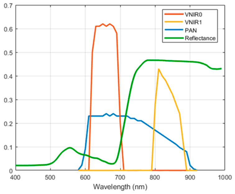
The SBG (Surface Biology and Geology) Thermal InfraRed (TIR) mission is a collaboration of the Italian Space Agency (ASI) with NASA/JPL (Jet Propulsion Laboratory) for the development of an Earth-observing satellite for the measurement and detection of land surface temperature and emissivity, evapotranspiration, snow properties, soil moisture, minerals, wildfires and volcanoes. The instrumental payload of the SBG-TIR satellite is composed of two instruments on the same rotating mirror. The thermal instrument, the Observing Thermal Emission Radiometer (OTTER), consists of a TIR multispectral scanner with six spectral bands operating between 8 μm and 12.5 μm and two mid-infrared bands at 4 μm and 4.8 μm, with a 60 m ground sample distance. The optical instrument, the Visible InfraRed Earth Observation camera (VIREO) consists of a two-band visible and near-infrared (VNIR) scanner operating at 655 nm (VNIR0 in the red spectral region) and 835 nm (VNIR1, in the near-infrared spectral region) with a 60 m ground sampling distance, together with a panchromatic band (PAN) centered at 750 nm and spanning 580–920 nm, providing a 30 m spatial resolution obtained from the native 60 m resolution through super-resolution. The full width at half maximum of the multispectral camera is 80 nm for VNIR bands and 300 nm for the PAN channel. The instrument field of view is ±34.4° and the overall swath is 935 km with a revisit time of less than 3 days. SBG-TIR can acquire images day and night and the local time descending node for the daily overpass is at 12:30.

One of the most important products of the mission is the real evapotranspiration (ET) computed at high spatial resolution. In this context, the exploitation of the data coming from the VIREO camera can allow the estimation of some vegetation parameters that represent key inputs for ET modeling. In particular, the Leaf Area Index (LAI, m²/m²) and the Vegetation Fractional Cover (FC, %) are crucial for a broad variety of land applications and for the modelling of ET.

The FC corresponds to the fraction of ground covered by green vegetation [1] and quantifies the spatial extent of the vegetation as projected at nadir. LAI indicates the one-sided leaf area per unit area of ground [2] and it is closely related to the transpiration process since it drives the actual green biomass. Both parameters are widely used to modulate surface albedo and surface emissivity, and for mixed pixels, it is possible to define a weighted function of the mixture components (e.g., vegetation and soil). The link between these vegetation structural parameters and thermal applications is well demonstrated [3,4], and this link opens synergies between VNIR and TIR cameras during the SBG-TIR space mission.

Indeed, the direct retrieval of the FC and LAI from the VIREO camera is very important in the context of the SBG-TIR mission, since it ensures co-registration with land surface temperature maps and eliminates geolocation errors, which is critical for applications relying on accurate evapotranspiration and surface energy flux estimates. It also reduces reliance on external data sources, minimizing the impact of cloud cover associated with the assimilation of data coming from other space missions. Moreover, it enables consistent retrievals across the sensor’s wide swath and facilitates synergistic use of VNIR and TIR observations throughout the mission. For these reasons, the development of an ad hoc algorithm to retrieve FC and LAI within the SBG-TIR mission is desirable. Although the SBG-TIR mission offers spectral bands in the red and near-infrared regions only, these are particularly effective for estimating biophysical parameters such as the LAI and FC since they contain most of the spectral information sensitive to structural variations in the canopy [5].

In recent years, various approaches based on satellite data have been developed to estimate LAI and FC from multispectral data. Retrieval methods based on the inversion of radiative transfer models (RTMs) have been used to generate operational biophysical products from Earth Observation data. For instance, the CYCLOPES products (Carbon cYcle and Change in Land Observational Products from an Ensemble of Satellites) [6] are derived from VEGETATION satellite data through inversion of the PROSAIL model. The MODIS (MODerate Resolution Imaging Spectroradiometer) LAI and Fraction of Absorbed Photosynthetically Active Radiation (FAPAR) products are based on a 3D RTM defined for eight biomes [7,8]. The GEOV1 products from Copernicus GEOland2 [9] are generated by fusing and scaling MODIS and CYCLOPES products using data from SPOT/VEGETATION and PROBA-V.

However, selecting the most appropriate algorithm requires careful consideration of the reliability of the estimated parameters and their associated uncertainties, considering expected accuracy, robustness, and timeliness for operational production [10]. These criteria tend to favor hybrid approaches based on machine learning techniques, which are computationally efficient, adhere to the physical principles embedded in RTMs, and are generally less prone to the convergence issues that affect physical inversion methods [11,12,13], often caused by the non-linearity of the inverse problem in remote sensing [14].

Hybrid methods combine the generalization capabilities of physical models with the accuracy and efficiency of non-parametric machine learning techniques [10,11,15,16]. Among these, neural networks have been implemented in operational processing chains to retrieve global biophysical parameters by inverting the PROSAIL model [6,17]. More recently, kernel-based algorithms have been introduced for classification and regression tasks in remote sensing [18]. Support Vector Regression has been applied to retrieve the LAI, FVC, and evapotranspiration [19,20], while GPR has demonstrated superior performance in LAI retrieval [21,22]. GPR is particularly effective in handling heterogeneous and noisy data and provides confidence intervals for its predictions. However, kernel-based machine learning approaches have not yet been implemented in operational retrieval chains for global-scale vegetation parameter estimation.

In this study, we explicitly reformulate the retrieval problem of the FC and LAI under SBG-TIR spectral constraints, where the availability of only three spectral bands severely limits spectral redundancy, and vegetation-background separability. The Soil Canopy Observation, Photochemistry and Energy Fluxes (SCOPE, [23]) radiative transfer model was used for the simulation of soil, leaf and canopy reflectance. The simulations were conducted in a wide range of viewing geometries and biophysical vegetation parameters. Then, different machine learning techniques were tested on simulated data, and the best-performing model was applied to Sentinel-2 imagery to validate model transferability and performance under real-world conditions. This ensures that the algorithms trained on synthetic simulations are robust under realistic observation conditions, capturing real-world variability and sensor noise. The novelty of this study lies in a rigorous retrieval framework designed for the low-dimensional spectral configuration of the SBG-TIR VNIR/PAN observations.

The proposed design ensures interpretability and operational flexibility, while providing actionable biophysical information to support applications ranging from agricultural management and forest monitoring to climate change studies. The methodology is fully transferable, allowing adaptation to other multispectral sensors, and lays a solid foundation for future large-scale and physically based retrievals of vegetation biophysical parameters.

2. Overall Methodology

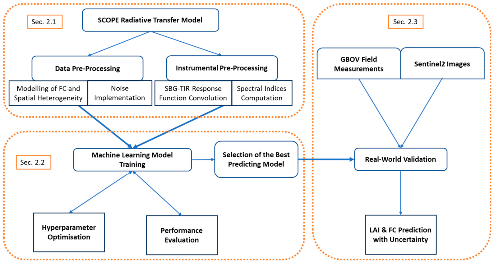
The overall procedure to retrieve the LAI and FC is outlined in Figure 1. Initially, the SCOPE radiative transfer model [23,24] was employed to simulate spectral signatures of soil, leaves, and canopy. SCOPE simulations were conducted over a wide range of viewing geometries, leaf and canopy vegetation parameters, soil optical and physical properties, and thermal variables.

By varying the initial conditions, a spectral library was constructed by pairing the simulated reflectance and thermal signals with the corresponding biophysical parameters. These spectra were then processed using the Instrument Spectral Response Function (ISRF) and then employed in the training phase of a machine learning algorithm aimed at solving the inversion problem, i.e., associating the biophysical variables with the given spectral information. Separate models were trained for each target parameter and subsequently tested on simulated data to identify the best-performing one in terms of accuracy and robustness, based on the synthetic dataset. The final models were then evaluated on Sentinel-2 images and the GBOV (Ground-Based Observations for Validation) data were used to validate the estimates. The following sections describe the workflow according to the scheme illustrated in Figure 1.

2.1. SCOPE Simulations and Pre-Processing

2.1.1. Model Description and Parameterization

SCOPE is a canopy-scale model that couples optical radiative transfer theory with models of photosynthetic activity and thermal emission. It is designed to simulate spectral reflectance, solar-induced chlorophyll fluorescence (SIF), and thermal emission in the VNIR and TIR domains. The model integrates the PROSPECT leaf model [25] and the SAIL canopy model [26], extending them with modules that account for key biochemical and physiological processes including stomatal regulation, leaf temperature dynamics, carbon assimilation, and xanthophyll cycle activity [23,24]. Within the SCOPE model, the leaf and canopy are represented as a one-dimensional (1D) turbid medium, where the electromagnetic radiative transfer equations are solved using a multi-stream approximation. In general, the 1D models assume that the canopy varies only with height above the ground surface and is horizontally homogeneous.

For each simulation run, a random sampling procedure was applied, where the input parameters were drawn from their respective probability distributions as defined in accordance with previous studies [27,28]. SCOPE input parameters used in the simulations are listed in

Table 1. Input parameters used for the simulations. Each parameter was sampled from its probability density function (PDF). Normal distributions are defined by their mean and standard deviation (Std); truncated normal distributions additionally include minimum (Min) and maximum (Max) bounds. Uniform distributions are specified only by their minimum and maximum values.

Category	Parameter	PDF	Min	Max	Mean	Std	Definition
Leaf	N	truncated gaussian	1.2	2.2	1.5	0.3	Leaf mesophyll structure parameter
	Cca	truncated gaussian	0	30	10	5	Carotenoid content (µg/cm2)
	Cdm	joint truncated gaussian	0.003	0.021	0.005	0.005	Dry matter content (g/cm2)
	Cw		0.005	0.035	0.02	0.006	Leaf water equivalent thickness (cm)
	Cab	joint uniform	0.01	80			Chlorophyll a and b content (µg/cm2)
Canopy	LAI		0.001	8			Leaf Area Index (m2/m2)
	LIDFa	joint uniform	−1	1			Leaf Inclination Distribution Function
	LIDFb		−1	1
	vCover	uniform	0	1			Vegetation spectral contribution
Soil	SMC	truncated gaussian	5	55	25	12.5	Soil moisture content in the root zone (%)
	BSMBrightness	truncated gaussian	0.01	0.9	0.5	0.25	BSM model parameter for soil brightness
	BSMlat	truncated gaussian	20	40	25	12.5	BSM model parameter ‘lat’
	BSMlon	truncated gaussian	45	65	50	10	BSM model parameter ‘long’
Geometry	tts (SZA)	uniform	0	60			Solar Zenith Angle (deg)
	tto (VZA)	uniform	0	36			View Zenith Angle (deg)
	psi (RAA)	uniform	0	180			Relative azimuth angle (deg)
Thermal	Ta	uniform	−5	45			Air temperature (°C)
	rs_thermal	uniform	0	0.1			Broadband soil reflectance in thermal range
	rho_thermal	uniform	0	0.1			Broadband thermal reflectance
	tau_thermal	uniform	0	0.1			Broadband thermal transmissivity
	Rss	uniform	1	3000			Soil surface evaporation resistance (s/m)

. Parameter domains were established based on empirical knowledge and designed to capture the heterogeneity of real-world scenes and to uniformly sample the hypercube of plausible experimental configurations [6,12]. The Gaussian distribution was used for most parameters, as it preserves the mean and standard deviation during the aggregation of variables describing both bare soil and vegetated surfaces [29]. In some cases, this distribution was truncated to ensure physical plausibility. The uniform distribution was used only when each value within the domain had an equal likelihood of occurrence.

Some parameters exhibit strong internal correlation. Specifically, the LAI and chlorophyll content (Cab) were sampled using a joint probability scheme, by partitioning the parameter space into four regions for each variable (Cab: 0–2, 5–20, 20–50, 50–80 µg cm⁻²; LAI: 0–0.2, 0.5–2, 2–5, 5–8), which were sampled with a uniform probability density function. For each sampled LAI region, Cab values were drawn from the corresponding subset, ensuring realistic combinations while avoiding implausible cases such as high LAI paired with very low Cab. For the remaining parameters, mutual correlations are often species- or context-dependent and therefore difficult to generalize; imposing joint probability structures could introduce artificial biases into the parameter space. Instead, additional plausibility constraints were applied to the leaf water content (Cw) and dry matter content (Cdm) to ensure realistic leaf composition: the leaf water fraction was constrained between 40% and 95%, reflecting typical values for green foliage [27]. Leaf orientation within the canopy was described using the Leaf Inclination Distribution Functions (LIDFa and LIDFb). LIDFa represents the mean leaf inclination angle, while LIDFb quantifies the variability around this mean orientation. Both parameters are constrained by geometric considerations to ensure that their sum does not exceed 1 [26], thus maintaining a physically realistic canopy structure. For soil parameters, no explicit constraints were applied. The ranges used were based on [30], simulating the effects of soil parameters on soil reflectance by modifying the model proposed in [31] using a statistical-based approach. For example, in the case of soil moisture content (SMC), the model directly generates realistic soil reflectance spectra for topsoil moisture contents up to 55% volumetric.

Geometric solar parameters (viewing and illumination angles) were defined according to the mission-specific observation geometry. Azimuth angles were treated as free parameters, although only the relative azimuth angle (RAA) significantly influences radiative transfer model outputs under the 1-D assumption [26]. Geometrical configurations are crucial due to the large off-nadir viewing geometry of the mission. Hence, we explicitly include Solar Zenith Angle (SZA), View Zenith Angle (VZA, constrained by the satellite’s 935 km swath width), and RAA (derived from the solar and sensor azimuth angles).

Soil spectra were generated using the Brightness–Shape–Moisture (BSM) module, while vegetation leaf spectra were computed via PROSAIL. These outputs were combined into a spectral library consisting of vegetation soil reflectance pairs associated with their respective input parameter sets. This allowed for the creation of a synthetic dataset representing the diversity of scenes expected during the satellite mission [27]. SCOPE outputs are provided at a high spectral resolution of 1 nm in the VNIR–Short-Wave Infrared Region (SWIR) range (400–2400 nm), at 0.1 µm resolution in the TIR range (2.5–15 µm) and 1 µm in the far TIR (15–50 µm). Reflectance in the VNIR-SWIR was computed as the ratio of reflected to incoming radiation (both direct and diffuse components).

The number of simulated spectra ($Ns$) varied between 500 and 12,000 to assess model performance and potential overfitting. In these simulations, the only source of variability was the random sampling of input parameters. Each simulation batch was initialized with a different predefined random seed ($\theta r$) to evaluate model robustness, avoid sampling bias and ensure reproducibility. The spectral library can thus be denoted as: $L(Ns,\theta r)$. Random numbers were generated using MATLAB 2022b’s built-in Mersenne Twister algorithm with varying seeds. This strategy ensured an even sampling on a logarithmic scale, allowing assessment of model sensitivity to the choice of library, and evaluation of the optimal training size by balancing computational cost and parameter space coverage while mitigating overfitting.

2.1.2. Fractional Cover Modeling

Since FC is not an input parameter of the SCOPE model and therefore cannot be directly estimated through inversion, a specific procedure was developed to incorporate this parameter into the modeling framework.

FC is related to the concept of gap fraction, which describes the probability of radiation not intercepting the canopy and reaching the ground [32]. Mathematically, the gap fraction can be expressed as $P(\theta )=\mathrm{e}\mathrm{x}\mathrm{p}[-LAI\cdot {\displaystyle \frac{G\left(\theta \right)}{cos\left(\theta \right)}}]$, where the LAI is the one-sided leaf area per ground area, and $\theta$ is the SZA. $G\left(\theta \right)$ represents the mean projection of the leaf normal vector along the solar direction and accounts for the Leaf Inclination Distribution Function (LIDF) within the canopy. Within SCOPE, the canopy is treated as a 1D turbid medium, implying a random distribution of leaves within the canopy volume [23] and a Poisson distribution is assumed [33]. $G\left(\theta \right)$ has been computed following [26,33,34] and it was obtained by integrating the absolute projection of the leaf normal vector along the solar direction over all possible leaf inclinations ($\phi$) and azimuths (ψ), weighted by the LIDF (Equation (1)). This means calculating how much the leaves “face” the sun on average, accounting for their typical orientation and considering the numerical values of the Gamma function (Γ). The Γ function terms represent the weighted average over the input parameters LIDF (a and b in Equation (1)) and it was computed for each SCOPE simulation.

$$G\left(\theta \right)=cos\left(\theta \right){\displaystyle \frac{\mathsf{\Gamma }\left(\frac{b+2}{2}\right)\mathsf{\Gamma }\left(\frac{a+b+3}{2}\right)}{\mathsf{\Gamma }\left(\frac{b+1}{2}\right)\mathsf{\Gamma }\left(\frac{a+b+4}{2}\right)}}$$

(1)

Usually, the extinction coefficient ($k$) in the Lambert–Beer law for transmittance (T) is defined as $k={\displaystyle \frac{G\left(\theta \right)}{cos\left(\theta \right)}}$, while T can be expressed as $T=exp\left(-k\cdot LAI\right)$. This approach has been well established in several previous studies [10,35,36] and it allows for FC estimation according to Equation (2):

$$FC=1-exp(-k\cdot LAI)$$

(2)

By implementing this procedure, FC can be computed by combining Equation (1) with the Lambert–Beer formulation, providing paired values of LAI and FC for each simulation. In this way, FC was effectively embedded within the SCOPE model.

FC and the LAI are conceptually related through this non-linear relationship. The LAI quantifies the vertical structure of the canopy, representing total leaf area per unit ground area and capturing canopy density and layering. FC represents the horizontal extent of vegetation at the ground within a pixel, derived from the LAI but reflecting areal occupancy rather than vertical complexity. This distinction allows simulation scenarios where the LAI is high even if vegetation covers only a small fraction of the ground, due to the influence of leaf angles in the LIDF.

2.1.3. Modeling Spatial Heterogeneity

Since the SCOPE model does not explicitly simulate variable mixtures of vegetation and bare soil, an additional mixing procedure was developed to better represent the spatial heterogeneity under real-world conditions [6,10]. A linear mixing model was therefore introduced to handle the representation of multiple surface components that may be present within a single pixel at a given spatial resolution. In this context, a variable vegetation fraction parameter (vCover) was introduced as a new model input to represent the fractional spectral contribution of vegetation to the overall pixel reflectance. The mixed reflectance spectrum R for each SCOPE simulation is then computed as

$$R=vCover\cdot Rveg+\left(1-vCover\right)\cdot Rsoil$$

(3)

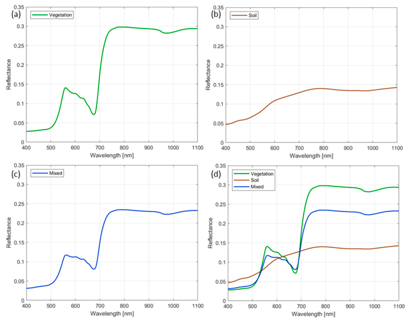
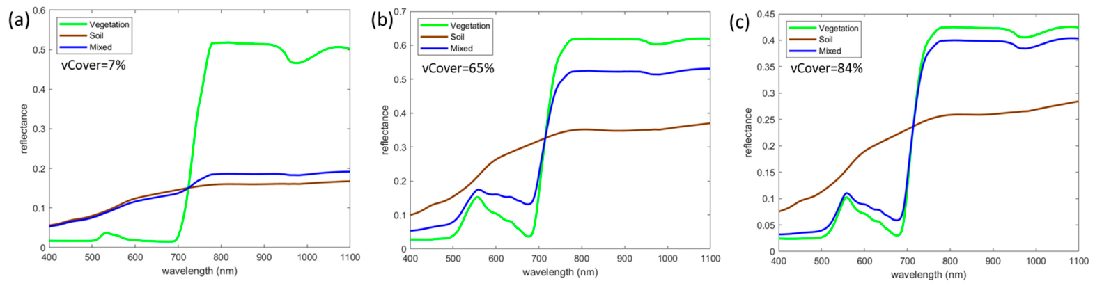
where $Rveg$ is the “pure” reflectance from vegetation, and $Rsoil$ is the “pure” reflectance from soil, with an example reported in Figure 2. The $Rsoil$ spectrum was scaled by the brightness coefficient (BSM Brightness in Table 1) to better represent variations in soil albedo, according to [6,28]. This approach accounts for background variability while limiting the number of parameters and avoiding unnecessary model complexity.

It is important to distinguish between vCover and FC. vCover is a pixel-scale mixing parameter used as an input in the SCOPE model to modulate the fractional contribution of vegetation and soil. FC, as described in Section 2.1.2, is a canopy-scale biophysical variable derived from gap fraction theory and depends on structural properties such as the LAI and leaf inclination distribution [37].

In summary, the proposed approach first simulates reflectance spectra using the SCOPE model and subsequently applies vCover to account for sub-pixel mixtures of vegetation and soil. The LAI parameter was then linearly rescaled according to the vCover values, under the assumption that bare soil exhibits LAI = 0. Therefore, pixel-level LAI becomes $LAImixed=LAIv\mathrm{\ast }vCover$, where $LAIv$ is the LAI used in each SCOPE simulation [6]. FC was subsequently derived consistently using the mathematical formulation defined in Section 2.1.2, applied to the $LAImixed$ values.

The final outcome was the generation of simulated spectra under heterogeneous conditions, thereby producing scenarios that are more representative of real-world surfaces.

2.1.4. Noise Implementation

Radiative transfer model simulations provide an idealized Top-Of-Canopy (TOC) signal. However, real sensor observations are affected by uncertainties arising from different sources, including: physical variability (e.g., clouds, adjacency effects), sensor limitations (e.g., calibration errors), scene heterogeneity at sub-pixel scale, as well as atmospheric, geometric, and radiometric corrections. To introduce realism and avoid overfitting, Gaussian white noise with variable intensity was applied to the reflectance obtained from Equation (3), acting as a regularization mechanism by relaxing the strict input–output mapping during training [38]. In line with [39], we implemented a wavelength-dependent multiplicative Gaussian noise model, $ϵ\left(\lambda \right)\sim N(0,{\sigma }^2)$, where $\sigma$ denotes the standard deviation controlling its magnitude. The noise model is defined as in Equation (4):

$$R\left(\lambda \right)=RSCOPE\left(\lambda \right)\cdot \left[1+ϵ\left(\lambda \right)\right]=RSCOPE\left(\lambda \right)+Rnoise\left(\lambda \right)$$

(4)

where $R SCOPE \left(\lambda \right)$ is the reflectance spectrum obtained from SCOPE simulations and $R noise \left(\lambda \right)$ represents the noise component in the resulting noisy reflectance spectrum ($R\left(\lambda \right))$. This noise model approximates realistic sensing conditions, since relative spectral shape is more important than absolute reflectance in retrieval tasks. The signal-to-noise ratio (SNR) is defined as [40] $SNR={\displaystyle \frac{Power\left(RSCOPE\right)}{Power\left(Rnoise\right)}}={\displaystyle \frac{1}{{\sigma }^2}}$.

For real-world multispectral instruments, SNR values vary across spectral bands. For instance, for Sentinel-2 the SNR in the visible range spans from 70 to 175 [41,42]. In this study, three noise levels were considered to assess model performance under varying observational uncertainty conditions: (i) no noise ($SNR=\mathrm{\infty }$); (ii) low-to-medium noise (SNR = 100), typical of operational satellite data; and (iii) high noise (SNR = 10), simulating severely degraded atmospheric or instrumental conditions. Statistically, these noise levels correspond to reflectance perturbations with 68% probability of falling within ±10% to ±33% of the original signal.

2.1.5. Dataset Resampling and Spectral Index Computation

Spectral reflectance was then resampled at the VIREO camera, using the ISRF of the VNIR0, VNIR1 and PAN (Figure 3). The reflectance values in these three optical channels were obtained by performing a discrete convolution between the SCOPE-simulated reflectance spectra R($\lambda$) and the ISRF of each channel (Figure 3). For a given channel C, the convolution is computed as $C=\sum R\left(\lambda \right)\cdot ISRF\left(\lambda \right)$.

After spectral resampling, a series of vegetation indices were computed to evaluate their contribution as additional inputs in LAI and FC retrieval. In particular, we tested the near-infrared reflectance of the vegetation index (NIRv), defined as the product of near-infrared reflectance and NDVI. NIRv is commonly used to approximate the fraction of pixel reflectance attributable to vegetation within a mixed pixel [43]. Moreover, it has been shown to better capture variations influenced by diurnal or weekly changes in canopy structure and function [44]. Finally, since daily temporal resolution was not considered in the simulation framework, NIRv may provide a useful proxy to reduce the influence of sub-daily variability when temporal resolution is limited to weekly or longer scales, as in the experimental validation dataset used.

The following six configurations (based on different input data) were considered to test the selected six machine learning models described in Section 2.2. The input data configurations considered in this study are: (i) VNIR0, VNIR1, SZA, VZA, and RAA; (ii) VNIR0, VNIR1, SZA, VZA, RAA, and NIRv; (iii) VNIR0, VNIR1, SZA, VZA, RAA, PAN, and NIRv; (iv) VNIR0, VNIR1, SZA, VZA, RAA, and PAN; (v) VNIR0, VNIR1, SZA, VZA, and RAA; and (vi) VNIR0, VNIR1.

2.2. Machine Learning Models, Training, Implementation, Validation and Uncertainty

2.2.1. Model Description

To explore a wide range of learning paradigms and assess their predictive capabilities, we tested six different supervised regression models based on machine learning: (i) decision tree regression (DT), (ii–iii) ensemble methods (Random Forest, RF; and Gradient Boosted Ensemble, specifically Least-Squares Boosting, LSB), (iv) kernel-based regression (Gaussian Process Regression, GPR), (v) Support Vector Machine (SVM), and (vi) neural network approaches (NN). This methodological diversity allows for a comprehensive evaluation of model performance across different regression strategies and provides insights into their generalization abilities in the context of vegetation biophysical parameter retrieval. Each model was optimized via Bayesian optimization over a problem-specific hyperparameter space as further described.

For DT-based models we controlled tree complexity through the minimum number of samples per leaf and the maximum depth. In RF we optimized the number of trees, the minimum leaf size, and the number of randomly selected features at each split. For LSB the learning rate, number of boosting iterations, and individual tree complexity were tuned. SVR models were implemented using a kernel function, with optimization of the kernel type, kernel scale (γ), box constraint (C), and ε-insensitive margin. GPR offers a probabilistic approach to regression, modeling the predictive map as a distribution over possible functions, providing both mean predictions and predictive uncertainty. We optimized kernel type, basis function, and noise level. We implemented an NN following a shallow feedforward architecture with up to 3 hidden layers, inspired by applications in vegetation biophysics [6]. The number of neurons, activation function, and regularization strength were optimized during the training.

Model performance was evaluated to identify the optimal input configuration and training dataset size Ns (the number of spectra). Thirteen values of Ns, ranging from 500 to 10,000 spectra, were tested to evenly sample the range and capture both low- and high-sample-size scenarios. For each Ns, spectral libraries were generated from a distinct configuration of the SCOPE input parameter set, obtained by randomly sampling the multivariate probability density function associated with their distribution. The random seed defining the number generation algorithm was fixed prior to sampling to ensure reproducibility. To evaluate the stability of the pipeline with respect to dataset variability, the experiment was repeated 11 times for each Ns using a different seed, resulting in a total of 143 libraries and approximately 800,000 spectra.

2.2.2. Training and Testing of Machine Learning Models

For each target variable, separate supervised models were trained. Within each spectral library $\mathrm{L}\left(\mathrm{N}\mathrm{s},\mathsf{\theta }\mathrm{r}\right)$, 80% of spectra were randomly selected for training and 20% for testing. Model performance was evaluated on the test set using the Root Mean Square Error (RMSE) and the coefficient of determination (R²).

Hyperparameters were optimized using a Bayesian optimization strategy with the cross-validation error as objective function. At each iteration, candidate configurations were proposed by an acquisition function (Expected Improvement Plus, which includes a penalization mechanism to avoid convergence to local minima). and evaluated using k-fold cross-validation on the training set. Once the optimal configuration is found, the model was retrained on the full training subset and then evaluated on the independent test set.

2.2.3. Model Performance Assessment and Robustness Analysis

Models’ robustness was evaluated with respect to variability arising from both the spectral simulations and the stochastic nature of the training process. Therefore, each model was trained and tested on each spectral library $L\left(Ns,\theta r\right)$. In addition, the machine learning algorithms are subject to internal sources of randomness (denoted by $\phi r)$, which affect: (i) the splitting of the dataset into training and test sets, (ii) the k-fold division, and finally, (iii) the optimization procedures (both parameter and hyperparameter learning). While the final selected model uses a fixed value for Ns, $\theta r$ and $\phi r$, the variability of these parameters was explored to assess model stability. It is worth noting that $\theta r$ is inherently stochastic and cannot be set a priori, as doing so would interfere with the generation of random numbers.

An iterative procedure was followed to train and test the six models across the six input data configurations. These ranged from minimal setups using only two visible-range features (VNIR0 and VNIR1) to richer configurations progressively including angular information (SZA, VZA, RAA), the PAN channel and the NIRv vegetation index. All features were independently normalized to the [0, 1] interval using min–max scaling, i.e., subtracting the minimum and dividing by the range of each feature. Prior analysis confirmed that model performance was not sensitive to the specific normalization method employed. For consistency and to isolate model performance from biases associated with absolute magnitudes, the target variables were mapped to the [0, 1] interval. For FC, this scaling is intrinsic by definition, whereas for the LAI, normalization was performed using the extreme values observed from the training set.

To evaluate the impact of feature dimensionality, a Principal Component Analysis (PCA) was implemented and tested as a dimensionality reduction method. However, given the relatively small number of input variables, PCA did not yield significant improvements in model accuracy and resulted in a slight increase in computational cost. Consequently, PCA was not adopted in the final models, in order to preserve model explainability.

2.2.4. Best Configuration Selection

The optimal Ns was identified by analyzing RMSE and R² as a function of Ns to determine the convergence point, beyond which observed differences are attributed to stochastic fluctuations rather than genuine performance improvements. This test was repeated across varying initial conditions, i.e., for different values of the randomness parameter $\theta r$ (as described in Section 2.1.1), producing a distribution of results rather than a single metric for each Ns. This approach provides statistical robustness for the assessment of model performance, ensuring that the identified optimal Ns is not an artifact of specific random initializations but reflects the true convergence behavior of the algorithm.

To identify the optimal Ns, group-wise comparison was performed using the Kruskal–Wallis (KW) test, suitable for independent groups with potentially non-Gaussian distributions. When statistically significant differences were detected (p-value < 0.05), the Dunn post hoc test (which uses the ranks from the KW analysis and includes a correction for multiple comparisons) was applied. By setting the significance level for each individual comparison to 0.05 divided by the number of comparisons, the overall Type I error is maintained at approximately 5%, ensuring statistically reliable results. The threshold of 0.05 was chosen as a conventional criterion for statistical significance, providing a practical balance between detecting meaningful differences and controlling false positives.

This same rank-based logic was extended to evaluate the comparability between distributions, allowing assessment of whether different feature configurations yield statistically equivalent performance. For the selection of the best variable set and model, training and testing were repeated for each configuration across the different randomness parameter values. This procedure produces a statistical sample of results per configuration, which can be visualized using boxplots showing the median (central value), interquartile range (IQR, 25th–75th percentile), and potential outliers, providing a robust characterization of variability. Using the median rather than the mean ensures that extreme values have a limited influence on the summary statistics.

2.2.5. Uncertainty Estimation

The explicit quantification of uncertainty has become a central requirement in remote sensing retrievals [45], as it enables a more reliable integration of biophysical parameters into data assimilation models, land surface schemes, and climate analyses. The trained models provide forward estimates of the target variables, which can be treated as realizations of random variables and thus described by a probability density function. Modern retrieval frameworks are expected not only to provide a single best estimate but also to characterize the confidence of their predictions, thereby enhancing interpretability and operational usability.

For some models, prediction uncertainty is inherently provided. For example, in GPR, uncertainty is typically expressed as the standard deviation of the posterior distribution. In this case, this intrinsic estimate naturally captures both types of uncertainty considered in our analysis using synthetic data. Aleatoric uncertainty is associated with the intrinsic variability in the data. In the context of the synthetic dataset, it includes instrumental noise, the variability obtained by mixing vegetation and soil spectra, and the natural variability of the simulated system not captured by the model (i.e., the random sampling of the probability distribution for each SCOPE biophysical input parameter). In contrast epistemic uncertainty originates from limitations of the model, such as structural assumptions, incomplete coverage of the input parameter space and also sensitivity to initialization. It reflects the confidence in the predicted values given the model formulation and the available training data. Together, aleatoric and epistemic uncertainties provide a comprehensive characterization of the reliability of model predictions [46].

For the other models, uncertainty was estimated through external procedures. Here, we exploited the bootstrap approach, which consists of repeatedly training the model on different bootstrap samples. Each bootstrap sample is generated by randomly resampling the original dataset with replacement, so some observations appear multiple times while others are omitted, producing a sample of the same size as the original dataset. The final prediction was then computed as the mean of the bootstrap predictions, while the associated uncertainty is estimated as the standard deviation across these outputs. This ensemble-based method captures only the epistemic uncertainty. To also account for the aleatoric component, we augmented the bootstrap-derived uncertainty with the empirical variance of the residual error observed on the training data. Let ŷ₁ denote the prediction of the b-th bootstrap model for a given input, and let μ be the mean of the prediction across all B bootstrap models. The total uncertainty for the bootstrap prediction (${{\sigma }_{tot}}^2)$ is given by the sum of the epistemic and aleatoric components and expressed in Equation (5):

$${{\sigma }_{tot}}^2={{\sigma }_{ep}}^2+{{\sigma }_{al}}^2={\displaystyle \frac{1}{B-1}}{\sum }_{i=1}^B(\widehat{{\mathrm{y}}_i}-\mathsf{\mu }{)}^2+{\displaystyle \frac{1}{N-1}}{\sum }_{i=1}^N{r_{\mathrm{i}}}^2$$

(5)

where N is the number of data points in the original (non-bootstrapped) training set used to train a single model for computing the residuals r_i. The first term ${{\sigma }_{ep}}^2$ represents the epistemic uncertainty, estimated from the variability of the bootstrap predictions, while the second term ${{\sigma }_{al}}^2$ represents the aleatoric uncertainty, estimated from the residuals of the model trained on the full dataset.

Evaluating the calibration of predicted uncertainties is essential to determine whether the model’s estimated confidence accurately reflects the true prediction errors. In other words, a well-calibrated uncertainty indicates that the predicted standard deviation corresponds to the observed variability between model outputs and reference values. To assess this calibration, we computed a normalized residual (t-statistic) for each prediction, defined as the residual divided by the estimated standard deviation. The resulting t-values were analyzed by plotting histograms and fitting several candidate distributions, namely Gaussian, t-Student, and Laplace distributions. A standard deviation of approximately 1 in the fitted t-Student distribution indicates that the estimated uncertainties are well calibrated, providing a stable and reliable measure of predictive error. Deviations from this value highlight potential under- or overestimation of uncertainty. In summary, while the intrinsic GPR uncertainty corresponds to the standard deviation of a Gaussian process, the bootstrap-derived uncertainty does not have a known probability density function a priori. However, if the number of bootstrap repetitions is sufficiently large, the Central Limit Theorem ensures that the distribution of predictions approaches a normal distribution. This justifies the use of the t-test to evaluate prediction accuracy and compute confidence intervals.

2.3. Application to Real Data

2.3.1. Sentinel-2 Images and GBOV Dataset

Once the best-performing model was selected based on the simulated data, it was subsequently applied to Sentinel-2 images and the estimates validated using the Copernicus GBOV service.

Given that the SBG-TIR mission is still in the preparatory phase we selected a satellite mission offering spectral characteristics that match as closely as possible to those used during training. The Sentinel-2 mission, developed and operated by ESA within the Copernicus Programme, provides globally consistent multispectral reflectance observations, making it particularly suitable for emulating the observational configuration of SBG. In particular, the VNIR0 and VNIR1 bands of the VIREO camera were spectrally resampled with Sentinel-2 bands B4 (RED, 665 nm) and B8 (NIR, 842 nm), respectively, with a spatial resolution of 10 m. The panchromatic band, which plays a key role in our model due to its coverage of the red-edge region, was reconstructed by combining multiple S2 bands within the relevant spectral domain. To derive the synthetic panchromatic band, we adopted a linear approximation method. Each Sentinel-2 band was modeled using a Gaussian response function using the central wavelength and full-width at half-maximum (FWHM). A discrete convolution between the Sentinel-2 response functions and the VIREO PAN spectral ISRF was performed to compute the weighted contribution of each band. The resulting synthetic PAN band was generated at a spatial resolution of 20 m, corresponding to the lowest native resolution of the input Sentinel-2 bands.

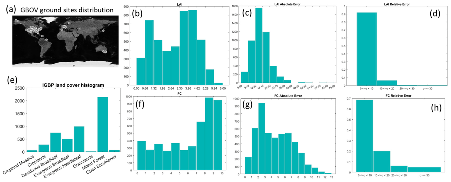
GBOV aims to develop and distribute robust in situ datasets for systematic and quantitative validation of Earth Observation (EO) land products. The dataset contains in situ reference measurements of vegetation biophysical parameters including the LAI and FC, with associated uncertainty. The selected dataset used in this study includes approximately 5000 measurements collected from 20 experimental sites across Europe, North America, and Australia, covering a wide range of soil types, vegetation covers, and different climatic zones. Each GBOV record is accompanied by precise spatial and temporal metadata, enabling direct spatial–temporal matching with satellite observations. For each ground measurement we extracted the corresponding Sentinel-2 (S2) images (from both platforms A and B) that included the point of interest and acquired within a ±3 days window around the GBOV measurement date. Both single-pixel extraction and neighborhood-based approaches (3 × 3 and 5 × 5-pixel buffers) were evaluated to mitigate the impact of sensor noise and sub-pixel heterogeneity.

A brief characterization of the experimental dataset is presented in Figure 4. The first panel shows the geographical distribution of the experimental sites, located across three different continents and covering multiple land cover classes, each represented with varying frequency. The two target variables, LAI and FC, are both well-defined within their theoretical ranges and each measurement is represented with the corresponding uncertainty value, whose distributions are illustrated in the histograms in Figure 4. In relative terms, the uncertainty-to-measurement ratio is below 20% for 90% of FC measurements and for 99% of LAI measurements.

We used 248 GBOV ground observations extracted from 98 different Sentinel-2 images, collected over a six-year period and covering five distinct and representative land cover types. This setup allows for a robust and representative evaluation of model performance under realistic observational conditions.

In summary, for each GBOV sample, a feature vector was constructed comprising three spectral bands (B4, B8, PAN), the NIRv vegetation index, and three solar and viewing variables (View Zenith Angle, sun zenith angle, relative azimuth angle). The dataset was then used as input to the trained models in predictive mode generating LAI and FC estimates under realistic observation geometries. The predictions were subsequently compared with the GBOV ground-truth and performance metrics including RMSE and R² were computed.

2.3.2. Comparison with Traditional Approach

In addition to our machine learning-based inversion, we applied the well-established benchmark model, the Sentinel-2 Biophysical Processor from ESA’s SNAP toolbox [47]. This processor relies on a neural network trained on PROSAIL radiative transfer simulations and requires the full set of Sentinel-2 spectral bands as input. Each biophysical variable (LAI, FC, etc.) is predicted by the same neural architecture but optimized with variable-specific weights.

Regarding the inputs, Sentinel-2 provides spectral bands at native spatial resolutions of 10, 20, or 60 m. Two versions of the processor are available: one exploiting only the 10 m bands and another operating at 20 m resolution, which also includes resampled versions of some 10 m bands. For our comparison, we selected the 20 m version, as it provides richer spectral information and includes the bands used to simulate the panchromatic channel in our dataset.

The comparison between our approach and the SNAP-based estimates was performed over the same spatial and temporal domains and conditions, ensuring a consistent benchmarking framework. Model performance was evaluated as prediction accuracy using the same error metrics (RMSE and R²) used during the best-model selection phase but computed between model predictions and GBOV ground-truth labels.

In addition, the analysis was conducted for different land cover types to assess model performance across diverse vegetation classes. Several regions of interest (ROIs) of varying sizes were tested to examine the influence of spatial representativeness on prediction accuracy.

3. Results

3.1. Simulated Dataset

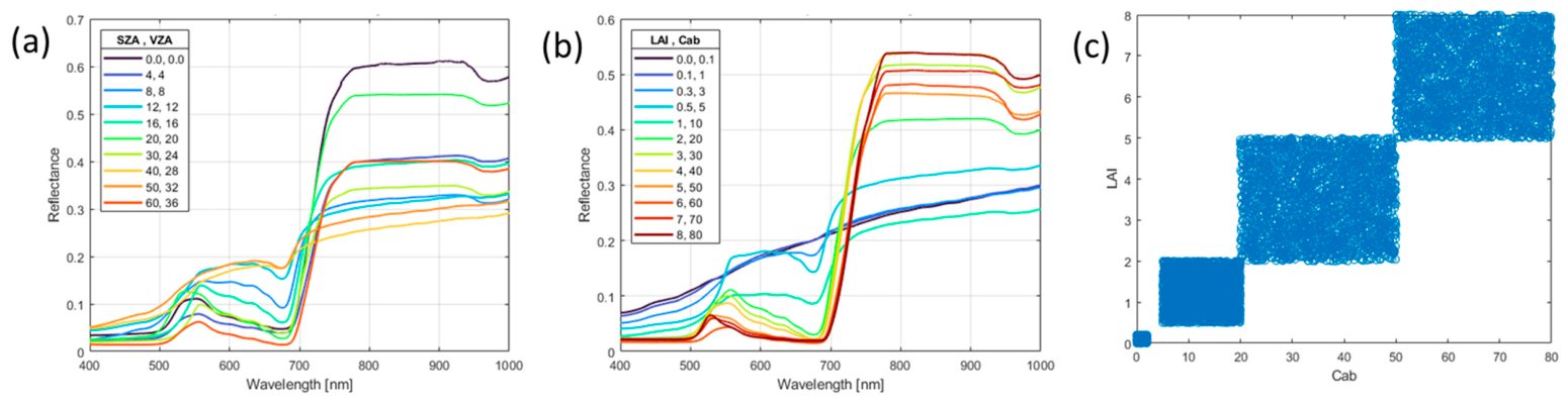
Figure 5 shows an example of the SCOPE simulated reflectance spectra for varying SZA and VZA and different combinations of LAI and chlorophyll content. The joint probability distribution between the LAI and Cab indicates the realistic combination of the vegetation parameters, avoiding implausible combinations.

Figure 6 shows the spectral reflectance obtained after applying the linear mixing model described in Section 2.1.3. When vCover is at its minimum (Figure 6a) the resulting spectrum closely resembles a bare-soil spectrum. For intermediate values (Figure 6b) both vegetation and soil components shape the spectral signature, producing a mixture of features such as partial absorption in the chlorophyll bands (~670 nm) and a subtle red-edge slope (~700 nm). Finally, when vCover is high (Figure 6c), the vegetation component dominates, and the spectrum exhibits the characteristic chlorophyll absorption and prominent red-edge transition associated with a fully vegetated canopy.

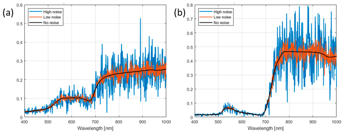
The multiplicative noise applied to the simulated spectra is shown in Figure 7. The resulting spectra, resampled to the SBG configuration, were used as input for the inversion. From Figure 7, it is evident that low noise levels (SNR = 100) slightly perturb the spectra without altering their overall shape. Variations are most pronounced in regions of high reflectance, such as the red-edge region, where multiplicative noise produces modest oscillations around the underlying trend. High noise levels (SNR = 10) induce stronger fluctuations; however, the overall spectral pattern remains preserved.

3.2. Machine Learning Inversion

In this section, we present the results of the machine learning model performance analyses. As described in Section 2.1.1, a total of 143 distinct spectral libraries were available for training, differing in random seed initialization ($\theta r$, 11 values) and the number of spectra (Ns, 13 values). Each spectrum was pre-processed and associated with seven predictive variables (VNIR0, VNIR1, SZA, VZA, RAA, PAN, NIRv) and two target variables (FC and LAI), which constitute the input–output pairs for the models. For each training run, one of the two targets was selected, and a single spectral library was used as input.

Several factors were systematically varied and optimized during training. Specifically, six different machine learning models were tested, along with six different combinations of predictive variables and three levels of added noise. The stability of each model was also evaluated with respect to the random seed to account for the intrinsic stochasticity of the training process.

3.2.1. Sample Size Sensitivity Analysis

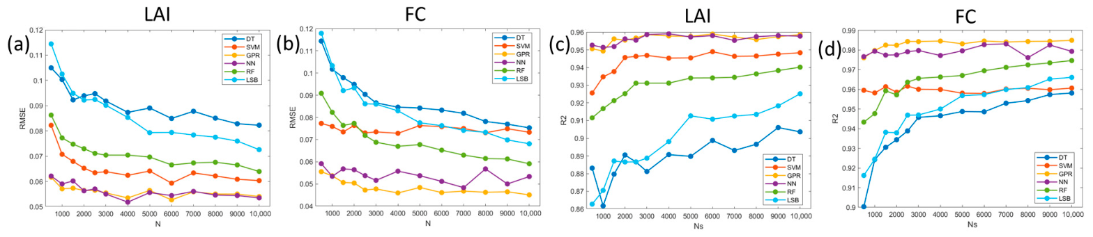
The first analysis aimed to investigate how the number of samples in the training dataset affects retrieval accuracy across all methods. The initial dataset consists of Ns spectra, of which 80% are used for training and the remaining 20% for testing model performance. Ns values ranged from 500 to 3000 with steps of 500, and from 4000 to 10,000 with steps of 1000. As presented in the method section, for each Ns, six different models were trained and evaluated by computing RMSE and R². Only the full set of variables was considered in this analysis, and no additional noise was added to the training spectra. Figure 8 shows the plots of the evaluation metrics as a function of dataset size.

The points shown correspond to median values computed across multiple dataset generated for each Ns, using different random seed ($\theta r$, Section 2.2.3), thereby accounting for stochastic variability in the data generation process. The use of the median ensures robustness against outliers.

The results indicate an almost constant trend of the metrics with increasing Ns, particularly for the two best-performing methods (GPR and NN). For all methods, performance is lower for Ns below 2000. Smaller than Ns = 500 datasets were excluded due to poor generalization performance. Overall, a rapid convergence of metrics is observed as Ns increases.

The KW test was applied to determine the optimal Ns on the GPR and NN models. This non-parametric approach is appropriate because 11 independent measurements per performance metric were available for each Ns, and no assumptions were made regarding the underlying distribution of data. The KW test returned a p-value < 0.05 indicating significant differences among the groups, and subsequent Dunn post hoc tests revealed that the first convergence point for Ns varies depending on both the model type and the evaluation metric, ranging between 1000 and 6000. To ensure consistency across models and to adopt a conservative approach that avoids potential bias from data selection, Ns = 6000 was chosen as a conservative training size for all subsequent analyses, as further increases in Ns would not substantially improve performance.

For numerical evaluation, the interquartile range (IQR) was associated with each metric. Reported values are consistently small, indicating stable predictions that are largely independent of the specific library spectra. In the noise-free case, the numerical metrics are as follows: for FC, RMSE = 0.046 (IQR = 0.002) and R² = 0.98 (IQR = 0.001); for the LAI, the best performance is RMSE = 0.053 (IQR = 0.005) and R² = 0.95 (IQR = 0.001), both obtained with the GPR model.

For SNR = 100, the results are nearly identical, with GPR again providing the best performance for FC, while the LAI exhibits a slightly larger IQR (0.005 for both RMSE and R²). Under high-noise conditions (SNR = 10) FC results are RMSE = 0.056 (IQR = 0.003) and R² = 0.977 (IQR = 0.002), while for the LAI the best results are RMSE = 0.063 (IQR = 0.006) and R² = 0.943 (IQR = 0.006).

Overall, while GPR provides slightly better median performance, the differences with NN are minimal and statistically comparable. Similarly, different feature configurations produce results close to those reported here.

3.2.2. Variable Selection and Preliminary Input Data Definition

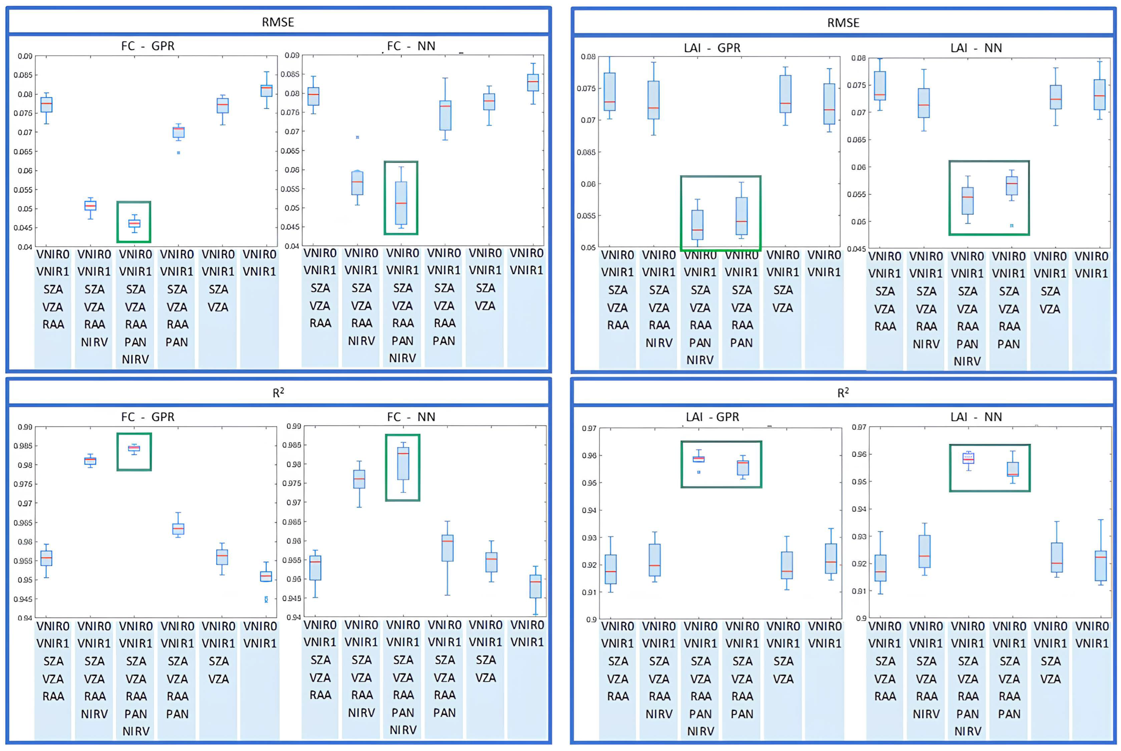
To further assess the stability of the results, boxplots of RMSE and R² for both GPR and NN were generated for different feature subsets (Figure 9).

As in the previous section, the boxplots were obtained by varying the random seed associated with training set generation. For this analysis, we restricted the comparison to the two best-performing models, GPR and NN. From Figure 9, it is evident that some feature configurations provide better statistical performance than others. Importantly, this conclusion does not depend on the metric considered (RMSE or R²), although the best-feature selection strongly depends on the target variable.

In both cases, the baseline configuration (RED, NIR + SZA, VZA, RAA) already provides satisfactory results. Adding further variables improves performance with the effect becoming particularly evident when introducing the PAN band for LAI estimation and the NIRv index for FC. The best overall performance is obtained when both variables are used together, confirming their complementary contribution to model accuracy.

When variables are removed no significant degradation is observed when excluding the mutual viewing geometry (RAA), while zenith angles (SZA and VZA) lead to a slight decrease in performance.

To select the optimal features configuration, the statistical KW test was performed between the two features subsets yielding the best performance in LAI prediction. The results indicate that selecting one subset over the other leads to statistically equivalent outcomes. For FC, however, a difference is observed: the improvement from baseline + NIRv to baseline + NIRv + PAN is statistically significant in the GPR model, with a median RMSE reduction from 0.052 to 0.046. This corresponds to an 11% relative decrease, which can be considered practically meaningful in terms of predictive performance improvement. The variability across repetitions remains low in both cases, with an IQR of approximately 0.002. Moreover, only 2 out of 13 repetitions show overlap in the distribution tails, indicating a consistent improvement across runs. Given the limited number of repetitions and the non-parametric nature of the analysis, emphasis was placed on distribution consistency and practical effect magnitude rather than on confidence interval estimation.

We selected this latter configuration for both variables, as it provides the best performance for FC and is among the top two configurations for LAI. Moreover, when comparing median values, it still yields the best results, even though, from a statistical standpoint, the difference cannot be asserted within a Type I error threshold (i.e., with less than a 5% probability of being wrong). It is also worth remarking that all the variables are available from the mission dataset.

This remains true across all SNR values and for both models. Some numerical results obtained with the full feature configuration, are reported in

Table 2. Test results for both RMSE and R² under two different SNR conditions. For each model the table reports the best median performance along with the interquartile range, corresponding to the best subset-of-features configuration. RMSE values are expressed as absolute percentages to enhance readability. The best-performing results in each case are underlined. A grey background highlights the statistic being referred to, while bold text indicates model and parameter names.

SNR Inf	RMSE%	DT	GPR	LSB	NN	RF	SVM	IQR%	DT	GPR	LSB	NN	RF	SVM
	FC	8.33	4.61	7.63	5.11	6.52	7.58	FC	0.17	0.20	0.22	1.12	0.28	0.34
	LAI	8.49	5.27	7.94	5.44	6.66	5.93	LAI	0.48	0.46	0.27	0.49	0.42	0.58
	R2	DT	GPR	LSB	NN	RF	SVM	IQR	DT	GPR	LSB	NN	RF	SVM
	FC	0.949	0.985	0.957	0.983	0.969	0.958	FC	0.004	0.001	0.004	0.008	0.002	0.004
	LAI	0.899	0.959	0.911	0.958	0.934	0.949	LAI	0.005	0.002	0.006	0.004	0.006	0.004
SNR 10	RMSE%	DT	GPR	LSB	NN	RF	SVM	IQR%	DT	GPR	LSB	NN	RF	SVM
	FC	8.82	5.58	8.17	5.58	6.86	7.91	FC	0.25	0.27	0.70	0.44	0.28	0.29
	LAI	8.81	6.35	8.69	6.34	6.86	7.05	LAI	0.64	0.49	0.51	0.54	0.52	0.63
	R2	DT	GPR	LSB	NN	RF	SVM	IQR	DT	GPR	LSB	NN	RF	SVM
	FC	0.949	0.985	0.957	0.983	0.969	0.958	FC	0.004	0.001	0.004	0.008	0.002	0.004
	LAI	0.899	0.959	0.911	0.958	0.934	0.949	LAI	0.005	0.002	0.006	0.004	0.006	0.004

for both the noise-free case $(SNR Inf = \mathrm{\infty }$) and the high-noise case (SNR 10). In the latter case (not shown as boxplots), the two methods perform equivalently. From the perspective of model performance, GPR appears more stable than the NN algorithm in terms of IQR when predicting FC, whereas no significant differences are observed in the IQR for LAI prediction.

3.2.3. Stability Analysis and Best Model Selection

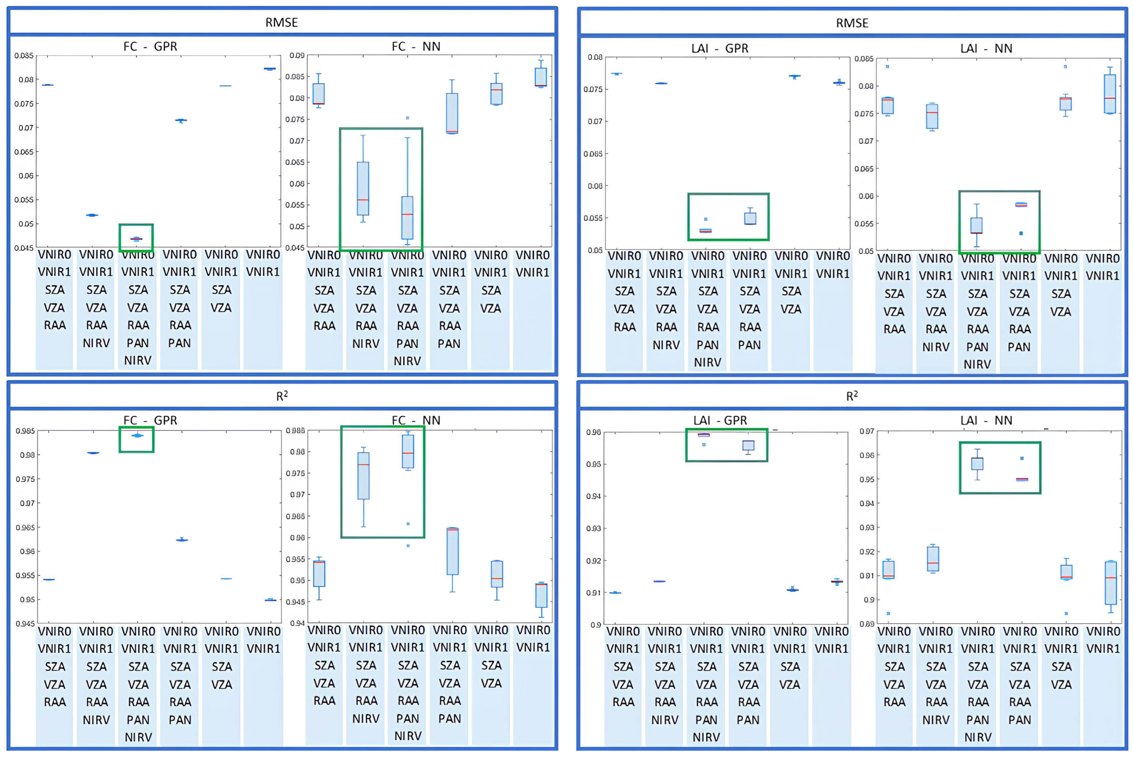
Two models, GPR and NN, were selected for further analysis because they exhibited comparable performance. To assess the results’ stability, the training and testing procedure was repeated while keeping the dataset fixed. During these repetitions the parameter $\phi r$ (described in Section 2.2.3), was varied; this parameter controls the randomness in the model training process, in contrast to θr, which governs the randomness in dataset construction and is kept constant in this analysis.

The boxplots obtained for different feature configurations are shown in Figure 10. The plots report the outcomes for both GPR and NN models under the previously selected feature configuration. GPR exhibits marked stability, whereas NN performance is strongly affected by randomness, resulting in less consistent outcomes that are highly dependent on the initial conditions. This behavior holds across different metrics and also when spectral noise is introduced (SNR = 10). Therefore, GPR was selected as the best-performing model, as it provides more stable results. Importantly, GPR not only delivers more stable predictions but also provides intrinsic estimates of uncertainty, which are more robust than the approach used for NN (see next Section 3.2.4). This combination of stability and uncertainty quantification represents a key methodological advantage, further justifying the selection of GPR as the preferred modeling approach.

3.2.4. Uncertainty Analysis

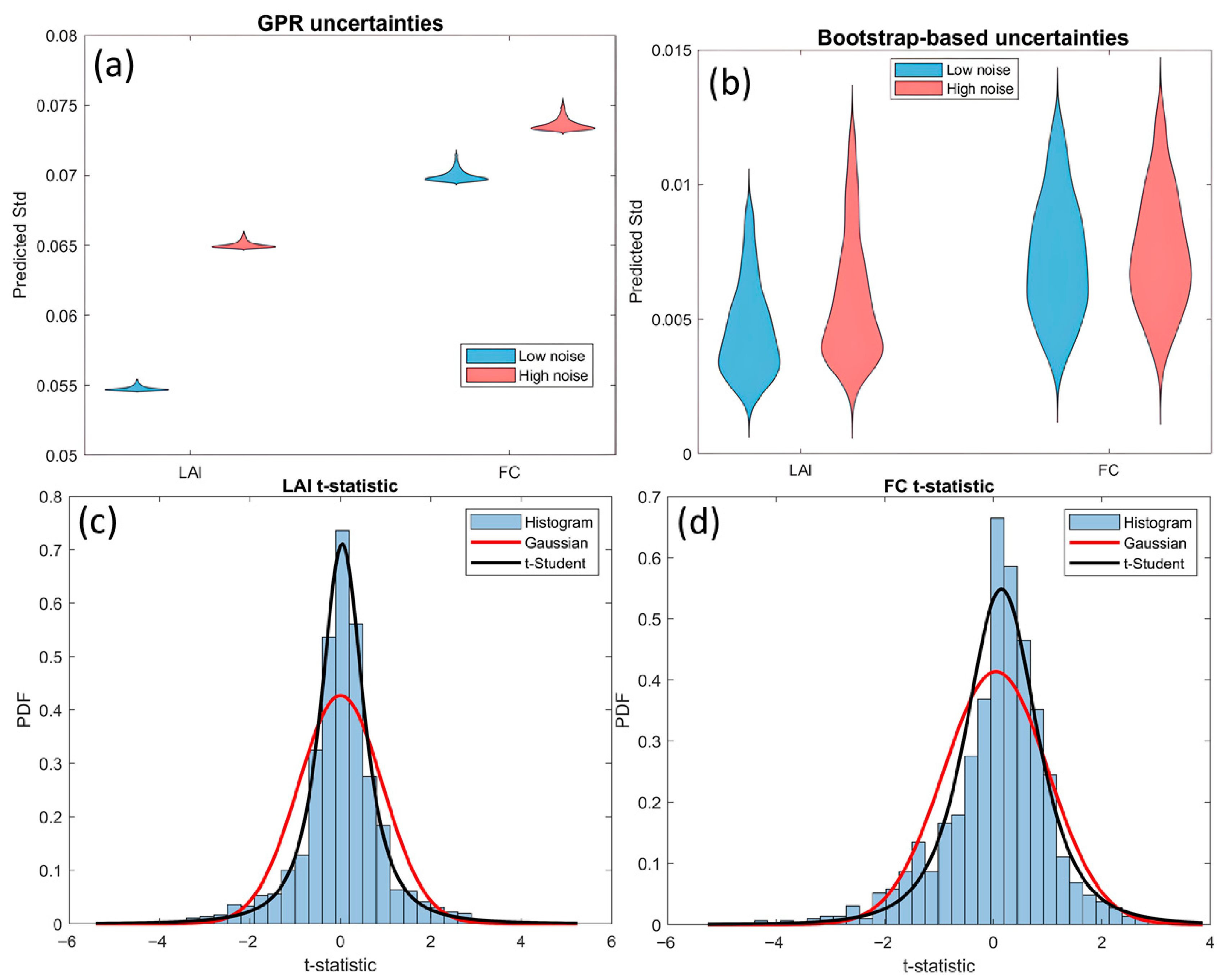
To quantify prediction uncertainty, we evaluated two approaches for the selected GPR model, as described in Section 2.2.4: bootstrap-derived uncertainty and intrinsic uncertainty. Figure 11a shows the violin plot of the uncertainty distributions obtained using the intrinsic GPR method. These plots combine a boxplot with a density estimate, providing visualization of both central tendency and overall spread. These distributions show a well-defined mode around a stable value (the horizontal line), with only a few outliers. For FC, the uncertainty is slightly higher than for the LAI, and in both cases, it increases when using the high-noise dataset. Figure 11b shows that the uncertainty distributions obtained from the bootstrap-based approach appear less concentrated around the mode and exhibit longer tails. Noise tends to further stretch the tails, although without producing significant visible effects. As expected, the absolute magnitude of bootstrap uncertainty is much smaller than the intrinsic estimates provided by GPR. This reflects the fact that GPR is highly stable, leading the bootstrap procedure to underestimate the effective confidence interval.

Figure 11c,d show the distributions of the t-statistic. Both histograms were fit to several candidate distributions, and in both cases, they were found to be well described by rescaled Student’s t distributions, with p-values of 0.56 and 0.47 for LAI and FC, respectively. When bootstrap-based uncertainties are used, the resulting t-values are excessively large compared to those obtained with GPR, confirming that bootstrap variance underestimates the effective uncertainty of the model. In contrast, the intrinsic GPR uncertainties yield residuals normalized with standard deviation close to 1, providing a more conservative and slightly overestimated measure of uncertainty, consistent with the residual spread.

The analysis of the mean values highlights different behaviors for the two target variables. For the LAI, the mean of the t-distribution deviates from zero by less than 5%, indicating that uncertainties are well calibrated relative to the residuals. For FC, residuals themselves are unbiased and centered on zero, but the normalized residuals (t-values) show a shifted mean. This suggests that while the predictions are unbiased, the estimated uncertainties are not perfectly calibrated, leading to systematic deviations in the normalized error distribution. From a numerical perspective, the t-statistic can be viewed as a rescaling of the residuals by an uncertainty value that remains approximately constant across predictions. Therefore, the bias observed in the FC t-distribution arises from a predominance of slightly overestimated predictions. The longer left tail corresponds to a small number of underestimated predictions. Nevertheless, the variance of the FC t-distribution is closer to 1 than that of the LAI, which can be interpreted as a smaller degree of uncertainty overestimation for FC.

In summary, the uncertainties estimated by GPR provide a reliable and conservative measure of predictive error, with good calibration for the LAI and a slight overestimation for FC. Bootstrap-based estimates tend to underestimate the model uncertainty; therefore, the intrinsic GPR uncertainties will be used in the final product.

3.2.5. Hyperparameter Optimization

The optimal hyperparameter configurations identified through the iterative Bayesian cross-validation strategy are reported in

Table 3. Hyperparameter configurations yielding the best performance for each model. Two SNR conditions, namely no noise and high noise (i.e., SNR = 10), are reported. Values were obtained through Bayesian hyperparameter optimization, with k-fold cross-validation used to iteratively update the objective function.

Algorithm	Hyperparameter	Range Values	Best LAI—Low Noise	Best FC— Low Noise	Best LAI— High Noise	Best FC— High Noise
Decision Tree Regression	Min Leaf Size	[1, 50]	44	6	25	6
	Max Depth	[10, 500]	234	414	72	438
Support Vector Regression	Box Constraint—C	[1 × 10−3, 1 × 103]	0.0012596	0.0012596	0.0012596	0.0012596
	Kernel Function	{gaussian, linear, polynomial}	linear	linear	linear	linear
	Kernel Scale	[1 × 10−3, 1 × 102]	0.0012173	0.0012173	0.0012173	0.0012173
	Epsilon	[1 × 10−3, 1]	0.014517	0.014517	0.014517	0.014517
Gaussian Process Regression	Basis Function	{constant, linear, quadratic}	constant	constant	constant	constant
	Kernel Function	{squaredexp, mat3/2, mat5/2}	squaredexp	squaredexp	squaredexp	squaredexp
	Sigma	[0.0030142, 1]	0.1876	0.1831	0.1876	0.063197
Shallow Fully- Connected Neural Networks	Number of Neurons	[5, 100]	66	39	29	69
	Number of Layers	[1, 3]	1	1	1	1
	Lambda	[1 × 10−5, 1 × 10−1]	2.12 × 10−5	2.13 × 10−5	2.15 × 10−5	1.23 × 10−5
	ActivationFunction	{relu, tanh, sigmoid}	relu	relu	relu	relu
Random Forest	Number of Trees	[10, 500]	485	18	464	17
	Min Leaf Size	[1, 50]	1	6	1	1
	Subsample fraction	[1, 7]	5	5	4	5
Least-Squares Boosting	Number of Trees	[50, 300]	124	124	124	124
	Min Leaf Size	[1, 50]	27	27	27	27
	Learning rate	[1 × 10−3, 1]	0.19523	0.19523	0.19523	0.19523
	NumVariables	[1, 7]	6	6	6	6

. For NN, the selected hyperparameters varied slightly across repetitions, due to the non-convexity of the hyperparameter space and high sensitivity to initial conditions. In contrast, GPR showed highly consistent hyperparameter selection, as the marginal likelihood surface is relatively smooth. Across all experiments, the GPR base function yielding the best performance was the constant function. This indicates that the predictive mean does not require a complex trend to model the relationship between inputs and target variables. Moreover, the squared exponential kernel is sufficient to capture the non-linear variations in the data. This resulted in minimal variability in model performance across repetitions and noise levels.

Overall, the hyperparameter optimization ensured that each model was evaluated under its best configuration, allowing a fair comparison of predictive accuracy and stability across both models and feature subsets. Additionally, the Bayesian optimization approach mitigates the risk of overfitting by efficiently exploring the hyperparameter space, leading to robust model performance across varying data subsets and noise conditions. By combining iterative hyperparameter tuning with cross-validation, each model was optimized while maintaining generalization capability, ensuring stability across repetitions and noise levels. The observed differences in stability between NN and GPR highlight the importance of model-specific hyperparameter tuning, especially for models sensitive to initial conditions.

3.2.6. Best-Case Results and Benchmarking

Before being applied to real satellite data, the best configurations identified were first evaluated on the independent test set to assess their generalization performance. The best configuration, as described in the previous sections, corresponds to the GPR model with the hyperparameters listed in Table 3. The training, validation, and testing phases were performed using a library of Ns = 6000 simulated spectra generated with the SCOPE model. All available variables were retained after the feature selection process. Consequently, in addition to the baseline feature set (RED, NIR, SZA, VZA, RAA), the PAN and NIRv indices were also included. When the model operates in predictive mode, all these variables must be provided as input data. Two independent algorithms were trained, one for each target variable (LAI and FC).

As shown in Section 3.2.1, results for the low-noise and no-noise cases were not significantly different. Therefore, the low-noise setup was selected for real-data application, as moderate noise slightly increased training variability and improved the representation of the irreducible (aleatoric) uncertainty, reducing overfitting.

The two random parameters, respectively controlling the initialization of the simulated library generation and the model training, were drawn once and then fixed. Otherwise, different random seeds could lead to variations in the learned parameters that would compromise the statistical validity and generalization capability of the model. Consequently, the resulting models represent those with the highest probability of achieving optimal performance metrics, as discussed in Section 3.2.2 and Section 3.2.3, rather than the absolute best values obtained by post hoc selection.

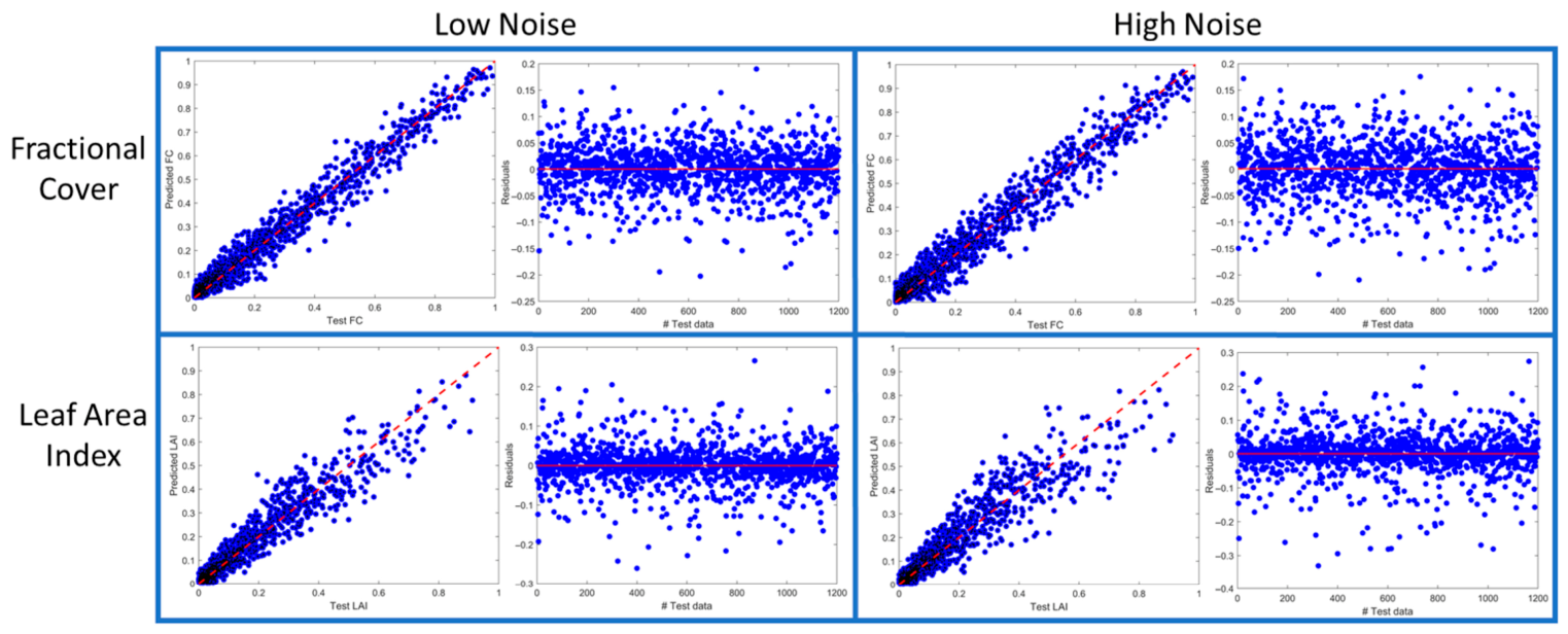
Figure 12 shows the results obtained for the four selected models. In the low-noise scenario (SNR = 100), the test-phase performance metrics were an RMSE of 0.052 and R² = 0.95 for the LAI, and an RMSE of 0.046 and R² = 0.98 for FC. Under high-noise conditions (SNR = 10), the corresponding results increased slightly, with an RMSE of 0.063 and R² = 0.93 for the LAI, and an RMSE of 0.054 and R² = 0.98 for FC.

These results indicate that FC predictions are slightly more accurate than those for the LAI, and that while high noise slightly affects performance, very high R² values are maintained for both variables. This behavior is consistent with results reported in previous studies. The obtained validation metrics are consistent with those in the literature.

It should be noted that LAI values were normalized to the [0, 1] range, as described in Section 2, to isolate model performance from biases associated with absolute LAI magnitudes. When applied to real data, predictions are rescaled using the inverse of the normalization relation. For comparison with other works, RMSE values were expressed as percentages. In some cases, where other studies did not follow this normalization procedure, their results have been rescaled using our relation and the minimum and maximum values reported in the corresponding references to enable a clear and consistent comparison across methods.

In [48] the model was trained on PROSAIL-simulated data using Sentinel-2A/B spectral response functions. Their best results were achieved with a neural network (one per target variable) using eight spectral bands and three geometric variables as inputs. Averaging the Sentinel-2A/B results, R² = 0.98 for FC (identical to ours), and R² = 0.82 for the LAI, slightly lower than our model. Their RMSEs are comparable: RMSE(FC) = 0.041 and RMSE(LAI) = 0.060 (after normalization to [0, 1] with reported LAI max = 15).

Similarly, in [10], the model was trained on PROSAIL-simulated data using the spectral response functions of the AVHRR optical channels. Their best model, a multi-output GPR, achieved R² > 0.88 across variables, in agreement with our results. Their reported RMSE(FC) = 0.043, slightly better than ours, while RMSE(LAI) = 0.081, slightly worse (already normalized).

3.3. Model Application to Sentinel-2 Data

As a result of the training and evaluation on synthetic datasets (Section 3.2), the best-performing and most robust models were selected for application to real observational data. A GPR model using the seven selected input variables (RED, NIR, SZA, VZA, RAA, PAN, NIRv) was used. Two separate single-output GPR models were trained, one for the LAI and one for FC. Each model was implemented under two noise conditions (low and high), reflecting the variability introduced during synthetic training, resulting in a total of four models applied to real-world measurements.

To ensure consistency, input parameters were defined according to the same configuration used during model training. Sentinel-2 imagery was used, with spectral bands reconfigured to match the SBG-TIR setup, as described in Section 2.3.2. The NIRv index was computed and the geometric parameters of the Sentinel-2 scene (SZA, VZA, RAA) were included. These inputs were then used to estimate the LAI and FC, and the results were compared with GBOV field measurements.

3.3.1. Validation on the GBOV Dataset

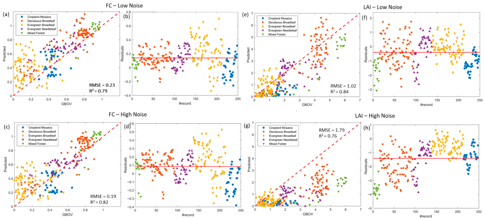
The scatterplots and residual plots comparing the Sentinel-2 modeled LAI and FC with GBOV field measurements are presented in Figure 13. In these scatterplots, the y-axis shows the model predictions while the x-axis represents GBOV field measurements. Overall, a clear decrease in performance is observed compared to the synthetic data, with considerable dispersion, as expected due to the complexity of real-world conditions.

Adding noise to the training data had contrasting effects on model performance. For FC, the inclusion of noise slightly improved predictions, reducing RMSE from 0.23 to 0.19 (Figure 13a,c). In contrast, LAI performance was substantially degraded, with RMSE increasing from 1.02 to 1.97 (Figure 13e,g).

Residual plots show the deviation between predicted and observed values on the y-axis. No pronounced trends were observed and bias levels were consistently low. Land cover-stratified analysis reveals clear patterns, with different classes clustering within specific value ranges. These distributions align with the seasonal timing of field data collection, which was primarily conducted during spring and summer. Systematic overestimation of FC is observed for evergreen broadleaf forests, and slight overestimation for deciduous broadleaf and mixed forest classes. These biases are mitigated by adding noise to the training data, reducing the mean residual bias (from 0.14 to 0.08) and also decreasing the number of predictions yielding non-physical values (i.e., exceeding 1). For LAI estimation, cropland and mixed forest tend to be underestimated, whereas deciduous broadleaf exhibits a high degree of variability.

To explore potential spatial effects on performance, we also tested ROIs of 3 × 3 and 5 × 5 sizes to evaluate whether spatial representativeness could affect the results, without observing significant differences in model performance. No significant differences were observed, which is both consistent and expected given that GBOV reference measurements [49] are point-based and Sentinel-2 imagery has a 20 m spatial resolution.

3.3.2. Comparison with SNAP Toolbox

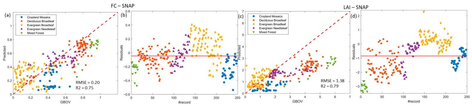
Machine learning results were compared with those obtained using the LAI/FC/FAPAR algorithm included in the SNAP toolbox [48]. Since the SNAP algorithm operates on full Sentinel-2 images, the LAI and FC values were extracted specifically for the same pixels and ROIs used to validate our models. This ensured a direct and consistent comparison between the GPR predictions and the SNAP outputs. The SNAP processor consistently underestimates LAI values across all land cover classes, whereas our proposed approach demonstrates improved performance on this dataset (Figure 14c,d). Regarding FC, both methods exhibit class-dependent clustering effects (Figure 14a,b). Evergreen broadleaf forests are generally overestimated, with SNAP showing a lower bias compared to our model. In contrast, mixed forest and deciduous broadleaf classes are slightly underestimated by SNAP, whereas our approach yields a mild overestimation. Cropland areas also tend to be underestimated by SNAP. Despite these differences, the overall bias remains limited.

Comparisons were conducted at the pixel level. Increasing the ROI size did not result in any significant improvement in model performance or correlation metrics, suggesting that spatial aggregation does not enhance the reliability of the retrievals in this context.

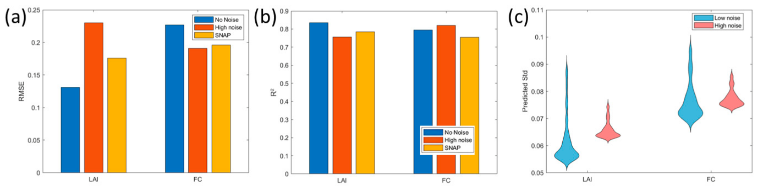
To further quantify model performance, Figure 15 presents a statistical comparison in terms of RMSE and R² for both the proposed model, evaluated under low- and high-noise configurations, and the SNAP Biophysical Processor. For LAI retrieval, the low-noise configuration of our model yields the highest accuracy, outperforming both the SNAP processor and the high-noise variant. Consequently, this configuration is recommended for LAI estimation within the SBG-TIR framework. In the case of FC, the inclusion of high noise in the training data produces results statistically comparable to those obtained with SNAP, indicating that this configuration is more suitable for FC retrieval in the same context.

Beyond the accuracy metrics, the uncertainty distributions, shown in Figure 15c, align well with theoretical expectations. When noise is introduced during training, the resulting uncertainty distribution becomes more concentrated, characterized by a higher mode and shorter tails.

A stratified analysis was performed to evaluate retrieval performance across different LAI ranges and land cover types. The corresponding quantitative results are reported in

Table 4. Statistical performance metrics for FC and LAI retrievals obtained from the stratified analysis. The left panel reports results stratified by LAI range (low and high), together with the comparison between the proposed SBG-TIR retrieval framework and the SNAP benchmark applied to the full dataset. The right panel shows retrieval performance stratified by different land cover classes.

Retrieval Performance Stratified by LAI	FC		LAI		Retrieval Performance Stratified by Land Cover	FC		LAI
	RMSE	R2	RMSE	R2		RMSE	R2	RMSE	R2
Low LAI (LAI < 2)	0.22	0.30	0.75	0.46	Cropland Mosaics	0.17	0.21	1.28	0.44
High LAI (LAI ≥ 2)	0.15	0.76	1.32	0.66	Deciduous Broadleaf	0.16	0.90	1.02	0.85
Full range (SBG-TIR)	0.19	0.82	1.02	0.84	Evergreen Broadleaf	0.25	0.15	0.67	0.33
Full range (SNAP)	0.20	0.75	1.38	0.79	Evergreen Needleleaf	0.14	0.54	1.08	0.13
					Mixed Forest	0.13	0.85	1.79	0.96

. When considering only experimental samples characterized by low LAI values (LAI < 2, selected with reference to Figure 5), FC retrieval accuracy is lower compared to the high-LAI regime. Conversely, LAI estimation shows the opposite behavior, with improved performance at low LAI and degraded accuracy at higher LAI values. In both cases, the best-performing models identified in the previous analysis were adopted: the low-noise training configuration for LAI retrieval and the high-noise injected configurations for FC retrieval. It is further observed that the coefficient of determination (R²) increases when the full dataset is considered, compared to retrievals performed on restricted LAI subsets. When trained and evaluated over the full range of conditions, the model effectively averages local biases, correlations, and RMSE that may dominate in narrower regimes. For completeness, Table 4 also reports a comparison with the configuration obtained using the SNAP benchmark processor. Retrieval performance also varies across different land cover types. In general, FC retrieval shows poorer performance over evergreen broadleaf forests, whereas LAI estimates remain acceptable for this class. Conversely, the best FC performance is observed over mixed forests and deciduous broadleaf forests, while the poorest LAI retrieval occurs in mixed forest areas. The R² values exhibit substantial variability across land cover classes, with deciduous and mixed forests being particularly well described by the model, indicating a stronger consistency between simulated and observed variability for these canopy types.

4. Discussion

4.1. Assumptions and Limitations of the SCOPE Simulation Framework

The simulated spectra generated in this study with the SCOPE model and using the proposed approach span a smooth transition from soil- to vegetation-dominated reflectance, providing a realistic representation of the variability that can occur in a single pixel in a natural landscape.

Alternative methodologies that employ three-dimensional (3D) RTMs, such as DART (Discrete Anisotropic Radiative Transfer [50]), may be more suitable for future applications aimed at improving FC estimation and linear mixing analysis. Although they are capable of representing complex canopy architectures, their advantages are reduced at SBG-TIR satellite pixel scale, where fine-scale effects are largely averaged. Moreover, the increased structural realism of 3D models requires higher computational costs and detailed ground-based measurements of both optical and structural vegetation properties [51]. Since under homogeneous conditions, 3D model outputs tend to converge toward those of one-dimensional (1D) models [29,52], a 1D radiative transfer approximation was adopted in this study, offering computational efficiency and simpler parametrization.

Within this framework, two simplifying assumptions were adopted: soil–vegetation mixing was modeled as linear, and surface elements were assumed to behave as Lambertian reflectors. Linear mixing represents a reasonable approximation at these satellite pixel scales and aligns with the assumptions of the SCOPE model. Non-linear soil–canopy coupling (e.g., via a multiplicative term in Equation (3), Section 2.1.3) could improve physical realism under very dense canopies, but the linear formulation was retained to avoid unnecessary model complexity. In this formulation, anisotropic reflectance effects, canopy clumping, and hotspot phenomena are not explicitly represented; however, efficient inversion and robust retrieval of the LAI and FC can be achieved using this approximation [26,53].

The inclusion of multiplicative, wavelength-dependent noise ensures that the simulated dataset better represents realistic measurement variability. This improves the generalization of retrieval algorithms trained on these spectra while preserving the physical integrity of the key spectral information. However, noise fluctuations are subsequently mitigated by the spectral convolution applied to derive sensor-level bands (see Section 2.1.5), which acts as a smoothing operation by averaging the signal within bands. As a result, local noise contributions are reduced while the main spectral features are preserved. Consequently, even under high-noise conditions, trends such as the increase in reflectance in the red-edge region associated with high-chlorophyll-content vegetation remain discernible.

At the same time, the level of noise introduced during training affects retrieval performance differently for each target variable. The LAI, being structurally driven, is more sensitive to added noise and is therefore more prone to degradation, whereas FC, being more directly related to broadband reflectance, may benefit from the regularizing effect of moderate noise, e.g., [32,54]. This behavior is also reflected in the predictive uncertainty, where higher noise leads to increased uncertainty that better captures the intrinsic (aleatoric) variability while reducing spurious fluctuations associated with epistemic uncertainty.

To ensure reproducibility, all simulations are generated using the explicitly defined parameter ranges reported in Table 1. The distributions of the individual parameters are sampled as described in Section 2.1.1, using fixed random seeds for both parameter sampling and noise generation. A separate random seed is used for the machine learning pipeline, including the train/validation split and the model training procedures (GPR and NN), ensuring full repeatability of the retrieval results. Under this configuration, all stochastic components are fully controlled and no variability remains across independent runs. Additional processing steps, such as linear mixing and spectral convolution to sensor bands, are fully deterministic given the same input data and random seed configuration.

4.2. Interpretation of Input Features in FC and LAI Retrieval

With regard to the retrieval performance obtained using simulated data, several observations merit further discussion. For both the LAI and FC, excluding angular information leads to a slight degradation in performance (Figure 9 and Figure 10), although the effect is moderate and not always statistically significant. This suggests that spectral variables (VNIR0 and VNIR1) already encode most of the information related to the biophysical parameters, while geometric variables (particularly SZA and VZA) play a supportive role. Their inclusion remains advisable, especially when dealing with real imagery, where illumination and observation conditions vary spatially and temporally [55,56].

From a physical perspective, the structural properties of vegetation are primarily encoded by the red and near-infrared regions of the spectrum, making VIREO bands essential inputs for both LAI and FC retrieval. However, the explicit representation of mixed-pixel effects introduces additional spectral variability that increases inversion complexity. To address this, NIRv is introduced as a partially redundant but informative feature that improves FC retrieval by isolating the photosynthetically active-vegetation signal [42], by partially removing background and illumination effects [57]. Previous studies [43] have shown NIRv to outperform NDVI in representing vegetation-related variability, particularly under conditions of mixed soil–vegetation cover and moderate to high canopy density. In contrast, the PAN band is particularly important for LAI estimation in heterogeneous conditions, as including the red-edge region it captures subtle variations in canopy chlorophyll content and structural variations [58]. In contrast, FC, being derived from the LAI according to Equation (2), tends to saturate in dense canopies [5] and is less sensitive to structural variability.

4.3. Consideration on GPR Performance

With regard to the retrieval pipeline, GPR was identified as the best-performing model for LAI and FC retrieval. Importantly, GPR not only delivers stable predictions but also provides intrinsic estimates of uncertainty, which are more robust than those obtained using NN (see Section 3.2.4.). This combination of stability and uncertainty quantification represents a key methodological advantage, supporting its selection as the preferred modeling approach.

The superior performance of GPR can be explained by the low-dimensional, physics-constrained input space, and the properties of kernel-based distance metrics. In the present low-dimensional 2 + 1 spectral band configuration, GPR benefits from meaningful distance calculation, whereas more flexible models such as Random Forests or neural networks rely on latent representations and higher computational cost to maintain performance. Additionally, NN performance exhibits higher fluctuations (Figure 10), which can be related to random weight initialization, while GPR provides stable predictions across different runs.

In addition, the smoothness imposed by the kernel function aligns naturally with the continuous and monotonic, physically constrained mappings generated by the SCOPE forward model. This implicit smoothness, combined with the limited and controlled parameter space (including the LAI-Cab relationship and the parametric LIDF), acts as a strong regularization mechanism, promoting robust generalization and reducing overfitting.

Although well-suited to low-dimensional settings, GPR can still perform competitively with additional spectral bands or sensors, as shown in [54], where it maintains predictive performance through the identification and removal of redundant spectral information.

An additional methodological aspect concerns whether the retrieval is performed jointly or separately for different target variables. Both approaches are valid: for example, ref. [48] adopts a separate retrieval strategy, whereas [10] implements a joint retrieval framework. These represent distinct methodological choices, and neither approach is intrinsically superior in principle. While joint retrievals can be formulated to avoid cross-parameter correlations, maintaining full control over the predictive pipeline through single-variable algorithms allows for clearer interpretation and a more direct association between each retrieved variable and its corresponding training labels.

The explicit incorporation of noise also serves as an implicit additional regularization, further enhancing model reliability. Moreover, recent studies have confirmed GPR uncertainty quantification as a benchmark for biophysical parameter retrieval [5].

Retrieval performance should also be evaluated in terms of predictive uncertainty [45]. In GPR, predictive uncertainty is primarily determined by the location of the input in feature space and the learned kernel structure, and does not directly depend on the absolute value of the target. Since FC is derived from the LAI via the gap fraction, it results in a non-linear mapping that compresses the data at high FC values, facilitating prediction (as visible in the scatterplot in Figure 12). As a result, the GPR predictive variance (based on input location in parameter space rather than the actual residuals) slightly overestimates uncertainty for FC, because the kernel variance still “sees” potential dispersion that the residuals do not exhibit. The residuals are therefore narrower and more tightly centered, leading to a minor overestimation of predictive uncertainty relative to the actual error. In contrast, the LAI is directly simulated and has a smoother, well-conditioned relationship with the inputs, resulting in well-calibrated GPR uncertainty (Figure 11c,d).

Additionally, inspection of the hyperparameters shown in Table 3 further illustrates this behavior. In response to the added noise, the optimized GPR noise parameter σₙ remained largely unaffected for the LAI, indicating limited adaptability to compensate for the perturbations. In contrast, for FC, σₙ exhibited a noticeable adjustment. This contrasting behavior can be explained by the nature of the perturbations, as the added noise introduces small fluctuations in the local parameter space explored during training, allowing the model to experience realistic variability. The GPR model is intrinsically robust to such variations, as it explicitly accounts for Gaussian noise through the relation ${\mathrm{y}}_i=\mathrm{f}\left({\mathrm{x}}_i\right)+{\mathsf{\epsilon }}_i$, where $ϵ\left(\lambda \right)\sim N(0,{{\mathsf{\sigma }}_{\mathrm{n}}}^2)$ with the noise variance σₙ² optimized as a hyperparameter.

4.4. Model Performance with Sentinel-2 Data and Comparison with Previous Studies

Overall, the retrieval performances obtained in this study are comparable to those reported in the literature, with comparable accuracy across methodologies. The slightly lower LAI performance in [10] can be attributed to the differences in spectral configuration. Our setup includes one band in the red, one in the NIR, and one covering both plus the red-edge region, whereas the configuration in [10] uses three different channels: one in the red, one spanning red-edge to NIR, and one in the SWIR (1.6 µm). The absence of separate bands capturing the rapid increase in vegetation reflectance in the red-edge and the subsequent plateau may explain the small accuracy gap. Supporting this observation, ref. [48] does not experience this limitation because their setup includes a larger number of spectral bands.

Moreover, a discrepancy between simulated and real data remains, representing the primary source of increased uncertainty when transitioning from synthetic to observed datasets. This highlights the intrinsic difficulty of reproducing real-world conditions using synthetic simulations, especially when validation relies on spectral features that may be slightly biased and not perfectly aligned with SBG characteristics. Performance is further constrained when accounting simultaneously for SBG and Sentinel-2 instruments’ configuration, due to differences in spectral response functions and acquisition conditions.

Additionally, several sources of uncertainty contribute to this domain gap. First, residual effects may arise from the atmospheric correction process, which can introduce biases or errors not fully captured in the synthetic dataset. For example, residual aerosol scattering or water vapor correction inaccuracies may slightly alter VNIR0 and VNIR1 reflectance values, propagating uncertainty into vegetation parameter retrievals. Second, although a Lambertian assumption was adopted within the synthetic simulation framework for consistency with the SCOPE 1D formalism, real Sentinel-2 observations may still exhibit anisotropic reflectance effects associated with BRDF variability that are not fully reproduced by the simulations. Third, the simplified one-dimensional representation of vegetation in SCOPE cannot fully capture the complexity of three-dimensional canopy structure, including shadowing and sub-pixel heterogeneity, which may further increase uncertainty.

A further source of uncertainty arises from the mismatch between point-scale in situ GBOV measurements [49] and pixel-scale Sentinel-2 observations at 20 m resolution. Although sensitivity analyses using different spatial aggregation windows (3 × 3 and 5 × 5 ROIs) did not reveal significant differences, this indicates that the signal is relatively stable within the considered spatial extent and that a 1-pixel representation is sufficient to capture local spatial variability. However, this does not remove the fundamental representativeness mismatch between point measurements, which can be regarded as infinitesimal samples within the pixel, and satellite observations, which integrate heterogeneous land surface conditions within a finite spatial support. This limitation becomes even more relevant in the context of the forthcoming SBG-TIR mission, which operates at a coarser spatial resolution of 60 m, where the larger pixel footprint is expected to further increase subpixel heterogeneity and therefore amplify scale-related representativeness errors in the validation and retrieval of biophysical parameters.

To mitigate all these limitations, approaches such as active learning (where the model iteratively selects the most informative real observations to refine the training set) or coupling synthetic data generation with atmospheric radiative transfer simulation (e.g., using MODTRAN) could be explored, potentially enhancing both predictive accuracy and robustness. Techniques such as noise injection, mixing, and the introduction of NIRv proved effective in reducing this gap and improving model performance. A further comparison between the two methods can be made in terms of their practical applicability and operational differences. While the two approaches share similar methodological foundations, some practical differences exist. The SNAP processor requires the full Sentinel-2 scene and a dedicated software environment, while our machine learning method can be applied directly to specific pixels of interest, offering greater flexibility and computational efficiency. Moreover, our machine learning-based inversion provides pixel-level uncertainty estimates, which are not available in SNAP. Conversely, the SNAP processor includes data quality flags based on likelihood analyses both within and across spectral bands, identifying pixels whose spectral signatures fall outside the training hypercube domain.

4.5. Stratified Analysis of Retrieval Performance

The stratified analysis provides additional insight into the behavior of the proposed retrieval model across different LAI regimes. When restricting the analysis to a specific domain (low or high LAI) and comparing it to the use of the full dataset, an increase in R² is observed in the full-range case. This behavior is expected because, from a statistical perspective, the model better explains the underlying variability of the data when evaluated across a broader range of conditions. In this configuration, local fluctuations that may dominate within restricted domains (such as regime-specific biases and variance) are effectively averaged out.

Additionally, when the model is trained and evaluated only on low-LAI samples, larger absolute deviations between predicted and reference values are observed. This reflects the inherent difficulty of estimating low LAI, which arises from two main factors. First, the model tends to learn the underlying canopy–radiation relationship more robustly at higher LAI values, where vegetation dominates the signal, while predictions at low LAI are more sensitive to noise and background effects. Second, under low-LAI conditions, similar vegetation spectra can correspond to different soil backgrounds, increasing spectral ambiguity. In contrast, at a high LAI, soil contributions are largely masked, reducing this degeneracy. For LAI retrieval, the degradation of performance in the high-LAI regime is primarily related to increased dispersion in the reference data, which is less pronounced for FC. In the case of FC, this dispersion is partially mitigated by its non-linear derivation from the LAI, which compresses variability at high canopy cover. As a result, FC retrievals exhibit a more stable behavior across regimes, while the LAI remains more sensitive to regime-dependent variability.

4.6. Novelty, Implications, and Perspectives

To summarize, it can be stated that the overall proposed approach lies in the integration of a physically based synthetic training framework with a dedicated end-to-end machine learning retrieval pipeline, specifically tailored to the spectral configuration of the SBG-TIR mission. A key feature of the proposed methodology is its explicit treatment of mixed-pixel conditions, wherein sub-pixel mixtures of soil and vegetation exert a significant influence on reflectance properties. To address this complexity, the framework incorporates the panchromatic channel, which captures broadband visible reflectance and enhances sensitivity to both soil and canopy brightness. This integration improves the model robustness to spatial heterogeneity and supports more accurate retrievals of biophysical parameters from both simulated and Sentinel-2 data. Furthermore, FC is explicitly derived here from canopy structural parameters simulated by the SCOPE radiative transfer model, ensuring a physically consistent definition that is directly linked to vegetation architecture rather than relying on empirical spectral proxies. This structural grounding enhances the interpretability and generalizability of the retrievals across different ecosystems and sensor platforms, as demonstrated using Sentinel-2 data resampled in the SBG-TIR configuration, making the approach particularly suitable for scalable application in upcoming missions such as SBG-TIR under limited ground-truth availability.

Importantly, while the individual components of the framework are based on established radiative transfer and machine learning methods, the methodological contribution of this work lies in their systematic integration under strongly constrained spectral conditions. In this setting, the inversion problem is defined not by novel individual components, but by their physically consistent coupling under low-dimensional spectral information, absence of SWIR data, and partial redundancy between PAN and VNIR spectral channels. This constraint-driven formulation requires a coherent linkage between canopy physical modeling, mixed-pixel representation, and uncertainty-aware regression, resulting in a retrieval strategy specifically adapted to the information-limited nature of the target sensor configuration.

While this study focuses on the accuracy of LAI and FC retrievals, it is important to recognize that errors in these parameters can propagate into downstream products, such as evapotranspiration and surface energy fluxes. For example, underestimation of the LAI can lead to systematic underestimation of canopy transpiration, since leaf area directly controls the total stomatal surface available for water vapor exchange. FC biases may alter the partitioning of net radiation between sensible and latent heat fluxes, thereby influencing the surface energy balance. For instance, ref. [59] observed that evapotranspiration is highly sensitive to variations in LAI compared to other variables such as surface albedo, highlighting the key role of leaf area in controlling canopy-scale water fluxes. Impacts on sensible heat flux exist but are generally more moderate. Future work could further quantify these effects within the context of SBG-TIR mission simulations.

Building on the results of this study, future work could focus on generalizing the retrieval framework to other satellite missions and sensor configurations beyond the VIREO VNIR/PAN setup.

5. Conclusions

In this study, we present a machine learning framework for the retrieval of the Leaf Area Index and Vegetation Fractional Cover in the context of the SBG-TIR mission. Multiple machine learning models were trained and validated using both SCOPE synthetic and real datasets. The optimal configurations were selected based on their consistent performance across varying initial conditions, including randomized parameters for synthetic library generation and training initialization. This strategy ensures robustness to training variability and enhances model stability with respect to data and parameter fluctuations.

Gaussian Process Regression emerged as the most accurate approach for both the LAI and FC. Specifically, the LAI model performed best under low-noise training conditions, while the FC model benefited from high-noise training, indicating that noise injection can act as an effective regularization strategy. A distinctive methodological contribution of this work is the explicit derivation of FC from leaf angle distribution, yielding results that are both biophysically meaningful and numerically consistent.

Seven input variables (RED, NIR, PAN, SZA, VZA, RAA, and NIRv) were utilized; however, sensitivity analysis revealed that the RED and NIR channels alone already provided high predictive accuracy, with marginal gains from additional variables.

The selected models were applied to Sentinel-2 imagery, demonstrating predictive behavior consistent with theoretical expectations and comparable to existing benchmarks. Mixed-pixel effects were essential for achieving reliable results on real-world data. In this context, the panchromatic channel proved particularly valuable, offering an integrative measure of the visible reflectance spectrum, enhancing sensitivity to soil reflectance, and improving the retrieval of biophysical parameters.

The primary innovation of this study lies in the tailored application of the framework to the SBG-TIR mission, given its specific spectral configuration and operational constraints. While individual components such as noise injection and mixed-pixel handling have been explored in previous research, this work integrates them into a coherent and operationally viable machine learning pipeline. In particular, the ambiguity introduced by mixed-pixel effects is addressed through the complementary use of the PAN channel for LAI retrieval and NIRv for FC estimation. The resulting framework enables accurate and robust retrievals of the LAI and FC and represents a transferable solution for deployment in SBG-TIR and future multispectral missions.

References

1. Bonham, C.D. Measurements for Terrestrial Vegetation; John Wiley & Sons, Ltd.: Chichester, UK, 2013. [Google Scholar] [CrossRef]
2. Chen, J.M.; Black, T.A. Defining Leaf Area Index for Non-Flat Leaves. Plant Cell Environ. 1992, 15, 421–429. [Google Scholar] [CrossRef]
3. Lin, X.; Wen, J.; Liu, Q.; You, D.; Wu, S.; Hao, D.; Xiao, Q.; Zhang, Z.; Zhang, Z. Spatiotemporal Variability of Land Surface Albedo over the Tibet Plateau from 2001 to 2019. Remote Sens. 2020, 12, 1188. [Google Scholar] [CrossRef]
4. Yin, C.L.; Meng, F.; Yu, Q.R. Calculation of Land Surface Emissivity and Retrieval of Land Surface Temperature Based on a Spectral Mixing Model. Infrared Phys. Technol. 2020, 108, 103333. [Google Scholar] [CrossRef]
5. Carlson, T.N.; Ripley, D.A. On the Relation between NDVI, Fractional Vegetation Cover, and Leaf Area Index. Remote Sens. Environ. 1997, 62, 241–252. [Google Scholar] [CrossRef]
6. Baret, F.; Hagolle, O.; Geiger, B.; Bicheron, P.; Miras, B.; Huc, M.; Berthelot, B.; Niño, F.; Weiss, M.; Samain, O.; et al. LAI, fAPAR and fCover CYCLOPES Global Products Derived from VEGETATION. Remote Sens. Environ. 2007, 110, 275–286. [Google Scholar] [CrossRef]
7. Myneni, R.B.; Hoffman, S.; Knyazikhin, Y.; Privette, J.L.; Glassy, J.; Tian, Y.; Wang, Y.; Song, X.; Zhang, Y.; Smith, G.R.; et al. Global Products of Vegetation Leaf Area and Fraction Absorbed PAR from Year One of MODIS Data. Remote Sens. Environ. 2002, 83, 214–231. [Google Scholar] [CrossRef]
8. Knyazikhin, Y.; Martonchik, J.V.; Diner, D.J.; Myneni, R.B.; Verstraete, M.; Pinty, B.; Gobron, N. Estimation of Vegetation Canopy Leaf Area Index and Fraction of Absorbed Photosynthetically Active Radiation from Atmosphere-corrected MISR Data. J. Geophys. Res. 1998, 103, 32239–32256. [Google Scholar] [CrossRef]
9. Baret, F.; Weiss, M.; Lacaze, R.; Camacho, F.; Makhmara, H.; Pacholcyzk, P.; Smets, B. GEOV1: LAI and FAPAR Essential Climate Variables and FCOVER Global Time Series Capitalizing over Existing Products. Part1: Principles of Development and Production. Remote Sens. Environ. 2013, 137, 299–309. [Google Scholar] [CrossRef]
10. García-Haro, F.J.; Campos-Taberner, M.; Muñoz-Marí, J.; Laparra, V.; Camacho, F.; Sánchez-Zapero, J.; Camps-Valls, G. Derivation of Global Vegetation Biophysical Parameters from EUMETSAT Polar System. ISPRS J. Photogramm. Remote Sens. 2018, 139, 57–74. [Google Scholar] [CrossRef]
11. Verrelst, J.; Muñoz, J.; Alonso, L.; Delegido, J.; Rivera, J.P.; Camps-Valls, G.; Moreno, J. Machine Learning Regression Algorithms for Biophysical Parameter Retrieval: Opportunities for Sentinel-2 and -3. Remote Sens. Environ. 2012, 118, 127–139. [Google Scholar] [CrossRef]
12. Verrelst, J.; Camps-Valls, G.; Muñoz-Marí, J.; Rivera, J.P.; Veroustraete, F.; Clevers, J.G.P.W.; Moreno, J. Optical Remote Sensing and the Retrieval of Terrestrial Vegetation Bio-Geophysical Properties—A Review. ISPRS J. Photogramm. Remote Sens. 2015, 108, 273–290. [Google Scholar] [CrossRef]
13. Camps-Valls, G.; Verrelst, J.; Munoz-Mari, J.; Laparra, V.; Mateo-Jimenez, F.; Gomez-Dans, J. A Survey on Gaussian Processes for Earth-Observation Data Analysis: A Comprehensive Investigation. IEEE Geosci. Remote Sens. Mag. 2016, 4, 58–78. [Google Scholar] [CrossRef]
14. Camps-Valls, G.; Svendsen, D.H.; Martino, L.; Muñoz-Marí, J.; Laparra, V.; Campos-Taberner, M.; Luengo, D. Physics-Aware Gaussian Processes for Earth Observation. In Image Analysis. SCIA 2017; Springer: Cham, Switzerland, 2017; pp. 205–217. [Google Scholar] [CrossRef]
15. Verger, A.; Baret, F.; Weiss, M. Performances of Neural Networks for Deriving LAI Estimates from Existing CYCLOPES and MODIS Products. Remote Sens. Environ. 2008, 112, 2789–2803. [Google Scholar] [CrossRef]
16. Houborg, R.; McCabe, M.F. A Hybrid Training Approach for Leaf Area Index Estimation via Cubist and Random Forests Machine-Learning. ISPRS J. Photogramm. Remote Sens. 2018, 135, 173–188. [Google Scholar] [CrossRef]
17. Bacour, C.; Bréon, F.-M.; Maignan, F. Normalization of the Directional Effects in NOAA–AVHRR Reflectance Measurements for an Improved Monitoring of Vegetation Cycles. Remote Sens. Environ. 2006, 102, 402–413. [Google Scholar] [CrossRef]
18. Pérez-Suay, A.; Amorós-López, J.; Gómez-Chova, L.; Laparra, V.; Muñoz-Marí, J.; Camps-Valls, G. Randomized Kernels for Large Scale Earth Observation Applications. Remote Sens. Environ. 2017, 202, 54–63. [Google Scholar] [CrossRef]
19. Yang, F.; White, M.A.; Michaelis, A.R.; Ichii, K.; Hashimoto, H.; Votava, P.; Zhu, A.-X.; Nemani, R.R. Prediction of Continental-Scale Evapotranspiration by Combining MODIS and AmeriFlux Data Through Support Vector Machine. IEEE Trans. Geosci. Remote Sens. 2006, 44, 3452–3461. [Google Scholar] [CrossRef]
20. Durbha, S.S.; King, R.L.; Younan, N.H. Support Vector Machines Regression for Retrieval of Leaf Area Index from Multiangle Imaging Spectroradiometer. Remote Sens. Environ. 2007, 107, 348–361. [Google Scholar] [CrossRef]
21. Lazaro-Gredilla, M.; Van Vaerenbergh, S. A Gaussian Process Model for Data Association and a Semidefinite Programming Solution. IEEE Trans. Neural Netw. Learn. Syst. 2014, 25, 1967–1979. [Google Scholar] [CrossRef]
22. Campos-Taberner, M.; García-Haro, F.J.; Camps-Valls, G.; Grau-Muedra, G.; Nutini, F.; Crema, A.; Boschetti, M. Multitemporal and Multiresolution Leaf Area Index Retrieval for Operational Local Rice Crop Monitoring. Remote Sens. Environ. 2016, 187, 102–118. [Google Scholar] [CrossRef]
23. Van Der Tol, C.; Verhoef, W.; Timmermans, J.; Verhoef, A.; Su, Z. An Integrated Model of Soil-Canopy Spectral Radiances, Photosynthesis, Fluorescence, Temperature and Energy Balance. Biogeosciences 2009, 6, 3109–3129. [Google Scholar] [CrossRef]
24. Yang, P.; Prikaziuk, E.; Verhoef, W.; Van Der Tol, C. SCOPE 2.0: A Model to Simulate Vegetated Land Surface Fluxes And satellite Signals. Geosci. Model Dev. 2021, 14, 4697–4712. [Google Scholar] [CrossRef]
25. Jacquemoud, S.; Baret, F. PROSPECT: A Model of Leaf Optical Properties Spectra. Remote Sens. Environ. 1990, 34, 75–91. [Google Scholar] [CrossRef]
26. Verhoef, W. Light Scattering by Leaf Layers with Application to Canopy Reflectance Modeling: The SAIL Model. Remote Sens. Environ. 1984, 16, 125–141. [Google Scholar] [CrossRef]
27. Lauvernet, C.; Baret, F.; Hascoët, L.; Buis, S.; Le Dimet, F.-X. Multitemporal-Patch Ensemble Inversion of Coupled Surface–Atmosphere Radiative Transfer Models for Land Surface Characterization. Remote Sens. Environ. 2008, 112, 851–861. [Google Scholar] [CrossRef]
28. Claverie, M.; Vermote, E.F.; Weiss, M.; Baret, F.; Hagolle, O.; Demarez, V. Validation of Coarse Spatial Resolution LAI and FAPAR Time Series over Cropland in Southwest France. Remote Sens. Environ. 2013, 139, 216–230. [Google Scholar] [CrossRef]
29. Frank, S.A. The Common Patterns of Nature. J. Evol. Biol. 2009, 22, 1563–1585. [Google Scholar] [CrossRef]
30. Verhoef, W.; Van Der Tol, C.; Middleton, E.M. Hyperspectral Radiative Transfer Modeling to Explore the Combined Retrieval of Biophysical Parameters and Canopy Fluorescence from FLEX—Sentinel-3 Tandem Mission Multi-Sensor Data. Remote Sens. Environ. 2018, 204, 942–963. [Google Scholar] [CrossRef]
31. Bach, H.; Mauser, W. Modelling and Model Verification of the Spectral Reflectance of Soils under Varying Moisture Conditions. In Proceedings of the IGARSS ’94—1994 IEEE International Geoscience and Remote Sensing Symposium; IEEE: Pasadena, CA, USA, 1994; Volume 4, pp. 2354–2356. [Google Scholar]
32. Weiss, M.; Baret, F.; Smith, G.J.; Jonckheere, I.; Coppin, P. Review of Methods for in Situ Leaf Area Index (LAI) Determination. Agric. For. Meteorol. 2004, 121, 37–53. [Google Scholar] [CrossRef]
33. Nilson, T. A Theoretical Analysis of the Frequency of Gaps in Plant Stands. Agric. Meteorol. 1971, 8, 25–38. [Google Scholar] [CrossRef]
34. Campbell, G.S. Extinction Coefficients for Radiation in Plant Canopies Calculated Using an Ellipsoidal Inclination Angle Distribution. Agric. For. Meteorol. 1986, 36, 317–321. [Google Scholar] [CrossRef]
35. Ding, Y.; Zheng, X.; Jiang, T. Comparison of Fractional Vegetation Cover Estimating Methods Using In-Situ Measurements and the PROSAIL Model. In Proceedings of the 2016 IEEE International Geoscience and Remote Sensing Symposium (IGARSS); IEEE: Beijing, China, 2016; pp. 4351–4354. [Google Scholar]
36. De Grave, C.; Verrelst, J.; Morcillo-Pallarés, P.; Pipia, L.; Rivera-Caicedo, J.P.; Amin, E.; Belda, S.; Moreno, J. Quantifying Vegetation Biophysical Variables from the Sentinel-3/FLEX Tandem Mission: Evaluation of the Synergy of OLCI and FLORIS Data Sources. Remote Sens. Environ. 2020, 251, 112101. [Google Scholar] [CrossRef]
37. Li, L.; Mu, X.; Jiang, H.; Chianucci, F.; Hu, R.; Song, W.; Qi, J.; Liu, S.; Zhou, J.; Chen, L.; et al. Review of Ground and Aerial Methods for Vegetation Cover Fraction (fCover) and Related Quantities Estimation: Definitions, Advances, Challenges, and Future Perspectives. ISPRS J. Photogramm. Remote Sens. 2023, 199, 133–156. [Google Scholar] [CrossRef]
38. Brede, B.; Verrelst, J.; Gastellu-Etchegorry, J.-P.; Clevers, J.G.P.W.; Goudzwaard, L.; Den Ouden, J.; Verbesselt, J.; Herold, M. Assessment of Workflow Feature Selection on Forest LAI Prediction with Sentinel-2A MSI, Landsat 7 ETM+ and Landsat 8 OLI. Remote Sens. 2020, 12, 915. [Google Scholar] [CrossRef]
39. Locherer, M.; Hank, T.; Danner, M.; Mauser, W. Retrieval of Seasonal Leaf Area Index from Simulated EnMAP Data through Optimized LUT-Based Inversion of the PROSAIL Model. Remote Sens. 2015, 7, 10321–10346. [Google Scholar] [CrossRef]
40. Schowengerdt, R.A. Remote Sensing: Models and Methods for Image Processing, 3rd ed.; Academic Press: Burlington, MA, USA, 2007. [Google Scholar]
41. Chambrelan, A.; S2 MPC Team. Sentinel-2 Level-1 Algorithm Theoretical Bases Document (ATBD); European Space Agency: Paris, France, 2023; Available online: https://sentiwiki.copernicus.eu/__attachments/1692737/S2-PDGS-MPC-ATBD-L1%20-%20Sentinel-2%20Level%201%20Algorithm%20Theoretical%20Bases%20Document%202023%20-%201.1.pdf?inst-v=19224347-b78a-4e98-8878-0bb2ef5b4589 (accessed on 19 December 2025).
42. Drusch, M.; Del Bello, U.; Carlier, S.; Colin, O.; Fernandez, V.; Gascon, F.; Hoersch, B.; Isola, C.; Laberinti, P.; Martimort, P.; et al. Sentinel-2: ESA’s Optical High-Resolution Mission for GMES Operational Services. Remote Sens. Environ. 2012, 120, 25–36. [Google Scholar] [CrossRef]
43. Badgley, G.; Field, C.B.; Berry, J.A. Canopy Near-Infrared Reflectance and Terrestrial Photosynthesis. Sci. Adv. 2017, 3, e1602244. [Google Scholar] [CrossRef] [PubMed]
44. Chen, S.; Zhao, W.; Zhang, R.; Sun, X.; Zhou, Y.; Liu, L. Higher Sensitivity of NIRv,Rad in Detecting Net Primary Productivity of C4 Than That of C3: Evidence from Ground Measurements of Wheat and Maize. Remote Sens. 2023, 15, 1133. [Google Scholar] [CrossRef]
45. Tran, B.N.; Van Der Kwast, J.; Seyoum, S.; Uijlenhoet, R.; Jewitt, G.; Mul, M. Uncertainty Assessment of Satellite Remote-Sensing-Based Evapotranspiration Estimates: A Systematic Review of Methods and Gaps. Hydrol. Earth Syst. Sci. 2023, 27, 4505–4528. [Google Scholar] [CrossRef]
46. Kendall, A.; Gal, Y. What Uncertainties Do We Need in Bayesian Deep Learning for Computer Vision? arXiv 2017, arXiv:1703.04977. [Google Scholar] [CrossRef]
47. Weiss, M.; Baret, F. ATBD_S2ToolBox_L2B_V1.1; INRAE: Montpellier, France, 2016; Available online: https://step.esa.int/docs/extra/ATBD_S2ToolBox_L2B_V1.1.pdf (accessed on 8 April 2026).
48. Weiss, M.; Baret, F.; Jay, S. ATBD_S2ToolBox_L2B_V2.0: S2ToolBox Level 2 Products LAI, FAPAR, FCOVER; INRAE: Montpellier, France, 2020; Available online: https://step.esa.int/docs/extra/ATBD_S2ToolBox_V2.0.pdf (accessed on 8 April 2026).
49. Bai, G.; Gobron, N.; Dash, J.; Brown, L.; Meier, C.; Lerebourg, C.; Ronco, E.; Lamquin, N.; Bruniquel, V.; Clerici, M. GBOV (Ground-Based Observation for Validation): A Copernicus Service for Validation of Vegetation Land Products. In Proceedings of the IGARSS 2019—2019 IEEE International Geoscience and Remote Sensing Symposium; IEEE: Yokohama, Japan, 2019; pp. 4592–4594. [Google Scholar]
50. Gastellu-Etchegorry, J.P.; Grau, E.; Lauret, N. DART: A 3D Model for Remote Sensing Images and Radiative Budget of Earth Surfaces. In Modeling and Simulation in Engineering; Alexandru, C., Ed.; InTech: London, UK, 2012. [Google Scholar]
51. Meroni, M.; Colombo, R.; Panigada, C. Inversion of a Radiative Transfer Model with Hyperspectral Observations for LAI Mapping in Poplar Plantations. Remote Sens. Environ. 2004, 92, 195–206. [Google Scholar] [CrossRef]
52. Banskota, A.; Serbin, S.P.; Wynne, R.H.; Thomas, V.A.; Falkowski, M.J.; Kayastha, N.; Gastellu-Etchegorry, J.-P.; Townsend, P.A. An LUT-Based Inversion of DART Model to Estimate Forest LAI from Hyperspectral Data. IEEE J. Sel. Top. Appl. Earth Obs. Remote Sens. 2015, 8, 3147–3160. [Google Scholar] [CrossRef]
53. Jacquemoud, S.; Verhoef, W.; Baret, F.; Bacour, C.; Zarco-Tejada, P.J.; Asner, G.P.; François, C.; Ustin, S.L. PROSPECT+SAIL Models: A Review of Use for Vegetation Characterization. Remote Sens. Environ. 2009, 113, S56–S66. [Google Scholar] [CrossRef]
54. Garrigues, S.; Lacaze, R.; Baret, F.; Morisette, J.T.; Weiss, M.; Nickeson, J.E.; Fernandes, R.; Plummer, S.; Shabanov, N.V.; Myneni, R.B.; et al. Validation and Intercomparison of Global Leaf Area Index Products Derived from Remote Sensing Data. J. Geophys. Res. 2008, 113, 2007JG000635. [Google Scholar] [CrossRef]
55. Verrelst, J.; Schaepman, M.E.; Koetz, B.; Kneubühler, M. Angular Sensitivity Analysis of Vegetation Indices Derived from CHRIS/PROBA Data. Remote Sens. Environ. 2008, 112, 2341–2353. [Google Scholar] [CrossRef]
56. Petri, C.A.; Galvão, L.S. Sensitivity of Seven MODIS Vegetation Indices to BRDF Effects during the Amazonian Dry Season. Remote Sens. 2019, 11, 1650. [Google Scholar] [CrossRef]
57. Gitelson, A.A.; Arkebauer, T.J.; Suyker, A.E. Convergence of Daily Light Use Efficiency in Irrigated and Rainfed C3 and C4 Crops. Remote Sens. Environ. 2018, 217, 30–37. [Google Scholar] [CrossRef]
58. Delegido, J.; Verrelst, J.; Alonso, L.; Moreno, J. Evaluation of Sentinel-2 Red-Edge Bands for Empirical Estimation of Green LAI and Chlorophyll Content. Sensors 2011, 11, 7063–7081. [Google Scholar] [CrossRef] [PubMed]
59. Peng, J.; Kharbouche, S.; Muller, J.-P.; Danne, O.; Blessing, S.; Giering, R.; Gobron, N.; Ludwig, R.; Müller, B.; Leng, G.; et al. Influences of Leaf Area Index and Albedo on Estimating Energy Fluxes with HOLAPS Framework. J. Hydrol. 2020, 580, 124245. [Google Scholar] [CrossRef]
Figure 1. Flowchart summarizing the main steps for FC and LAI retrieval. Details are provided in Section 2.1, Section 2.2 and Section 2.3.
Remotesensing 18 01931 g001
Figure 2. Linear mixing model scheme. To better represent the reflectance spectrum of a real pixel, the vegetation and soil spectra were linearly combined using a weighted average controlled by the parameter vCover. The (a) panel shows the vegetation spectrum, the (b) panel the soil spectrum, the (c) panel the resulting mixed spectrum, and the (d) panel the three spectra displayed together. The example shown corresponds to vCover = 0.66.
Remotesensing 18 01931 g002
Figure 3. SBG-TIR spectral response functions in the optical domain, showing three main channels: VNIR0 (RED region), VNIR1 (near-infrared, NIR), and the panchromatic (PAN) band. The green line represents an example of a simulated vegetation spectrum.
Remotesensing 18 01931 g003
Figure 4. The first panel (a) reports the geographical distribution of the experimental sites together with the associated land cover classes (e). Adjacent histograms illustrate the distributions of the two target variables, LAI (b) and FC (f), along with their corresponding uncertainty (c,g) and relative error distributions (d,h).
Remotesensing 18 01931 g004
Figure 5. Simulated reflectance spectra illustrating the combined effects of observation geometry and biophysical parameters. (a): Variations in reflectance induced by changes in Solar Zenith Angle (SZA) and View Zenith Angle (VZA), highlighting geometric effects on canopy–sensor interactions. (b): Spectral variability associated with different combinations of Leaf Area Index (LAI) and chlorophyll content (Cab), showing the influence of canopy structure and leaf optical properties. (c): Distribution of Cab and LAI parameter pairs.
Remotesensing 18 01931 g005
Figure 6. Simulated mixed reflectance spectra obtained using a linear mixing model of vegetation and soil components. The parameter vCover represents the fractional contribution of vegetation in the mixture. (a): A soil-dominated spectrum, where reflectance is primarily influenced by the soil component. (b): A mixed spectrum in which both vegetation and soil contribute significantly. (c): A vegetation-dominated spectrum, where the reflectance is largely determined by the vegetation component.
Remotesensing 18 01931 g006
Figure 7. Simulated canopy reflectance spectra for two distinct base reflectance cases (a,b), each with three noise levels: Low noise corresponds to a signal-to-noise ratio (SNR) of 100. High noise corresponds to SNR = 10.
Remotesensing 18 01931 g007
Figure 8. Performance metrics as a function of the number of spectra (Ns). (a,b) panels show RMSE for the LAI and FC respectively, while (c,d) show R2 for the LAI and FC, respectively. Results are shown for all selected methods, without added noise to the reflectance. Each point represents the median of results obtained from models trained on 11 different training sets.
Remotesensing 18 01931 g008
Figure 9. Boxplots of performance metrics summarizing results from 11 different training sets, used to evaluate the impact of training set variability on model stability. The x-axis shows different feature subsets, starting with the baseline configuration that includes the two spectral variables (VNIR0 and VNIR1) plus three geometric variables (VZA, SZA, RAA), shown as the first configuration in each plot. The variables are then added or removed to assess feature selection effects. Four pairs of plots are presented, each pair comparing GPR (left) and NN (right) models. The (top) pairs show RMSE, while the (bottom) pairs show R2; FC is displayed on the two (left) pairs, the LAI on the (right) ones. The best-performing configurations from a statistical perspective are highlighted in green. In the boxplots, the horizontal red line indicates the median, the whiskers represent the range of non-outlier values, and the cross markers indicate outliers.
Remotesensing 18 01931 g009
Figure 10. Boxplots of performance metrics obtained by training the selected model 11 times with different initial random conditions, used to evaluate the stability of the results with respect to the training procedure. As in Figure 9, the x-axis shows different feature subsets, starting with the baseline configuration that includes the two spectral variables (VNIR0 and VNIR1) plus three geometric variables (VZA, SZA, RAA), shown as the first configuration in each plot. The variables are then added or removed to assess feature selection effects. Four pairs of plots are presented, comparing GPR (left) and NN (right) models. The (top) pairs show RMSE, while the (bottom) pairs show R2; FC is displayed on the (left), the LAI on the (right). The best-performing configurations from a statistical perspective are highlighted in green. In the boxplots, the horizontal red line indicates the median, the whiskers represent the range of non-outlier values, and the cross markers indicate outliers.
Remotesensing 18 01931 g010
Figure 11. Uncertainty-related plots. The two top panels (a,b) show violin plots of the estimated uncertainties over the test set: GPR-based (left,a), bootstrap-based (right,b). For both LAI and FC, the distributions are stable around the mode (with respect to labels normalized between 0 and 1), and results are reported for two different SNR conditions (low, SNR = 100 and high, SNR = 10). The bottom panels show histograms of the t-statistics computed from the GPR-based residuals of the test set: (c) the LAI on the left, (d) FC on the right. Gaussian and Student’s t best-fitting distributions are shown.
Remotesensing 18 01931 g011
Figure 12. Application of the best model to the unseen test set. Scatter plots and residual are presented for FC (top) and the LAI (bottom), with low-noise and high-noise conditions shown on the (left) and (right) side, respectively.
Remotesensing 18 01931 g012
Figure 13. Sentinel-2 data analysis for FC (left) and the LAI (right). The scatterplots for low-noise (a,e) and high-noise (c,g) cases are shown, while panels (b,f) and (d,h) display the corresponding residual plots. Different colors represent the investigated land cover.
Remotesensing 18 01931 g013
Figure 14. Real-data testing results for the SNAP Biophysical Processor. Scatterplots and residual plots are shown for the LAI (a,b) and FC (c,d), based on Sentinel-2 pixels corresponding to GBOV reference points.
Remotesensing 18 01931 g014
Figure 15. Performance comparison on real data. (a): Bar plots of RMSE for LAI and FC predictions validated against the GBOV dataset, under three conditions (no noise, SNR = 10, SNAP Biophysical Processor). (b): The same bar plots for R2. (c): A violin plot of the estimated uncertainties.
Remotesensing 18 01931 g015