High-Accuracy Remote Sensing Identification of Winter Wheat Based on Feature Selection and Cross-Temporal Fusion in Shandong Province, China

Highlights

What are the main findings?

• Growth-stage ranking and key spectral variable selection effectively reduced the original 64-dimensional feature space to 16 informative variables.
• The cross-temporal fusion model achieved high winter wheat identification accuracy (OA = 0.9658, UA = 0.9609) using only 10 fused features.

What are the implications of the main findings?

• Cross-temporal feature fusion provides a more efficient alternative to direct stacking of multi-temporal remote sensing features.
• The proposed framework supports reliable 10 m regional-scale winter wheat mapping with strong consistency with statistical data.

Abstract

Accurate crop distribution mapping using multi-temporal remote sensing has become increasingly important for agricultural monitoring and management. However, existing methods often rely on the direct stacking of multi-temporal features, which leads to feature redundancy and reduced model efficiency. To address this issue, this study proposes a winter wheat identification framework that integrates growth-stage ranking, key spectral variable selection, and cross-temporal feature fusion. Taking Shandong Province as the study area, eight typical growth stages during the 2023–2024 winter wheat growing season were analyzed using Sentinel-2 imagery. Random Forest models were first constructed for each growth stage to evaluate discriminative ability. Then, spectral variable contributions were quantified using permutation importance, and key spectral variables were selected under correlation constraints. The progressive accumulation model (PAM) was then developed according to the ranking of discriminative ability across different growth stages, while the cross-temporal fusion model (CTFM) was constructed by extracting inter-stage mean values (mean) and inter-stage differences (diff) of key variables. The results show that the feature space was reduced from 64 dimensions (8 stages × 8 variables) to 16 key variables, substantially improving feature representation efficiency. Among the eight growth stages, the jointing, overwintering, heading, and grain-filling stages exhibited relatively strong discriminative ability. In the cross-temporal experiments, CTFM M6, which integrates information from the top six growth stages ranked by discriminative ability, achieved an overall accuracy (OA) of 0.9658 and a user’s accuracy (UA) of 0.9609 using only 10 fused features, providing the best balance between identification accuracy and feature dimensionality. Based on this model, a 10 m resolution winter wheat distribution map of Shandong Province was generated, and the estimated planting area showed high consistency with statistical yearbook data. These results demonstrate that the proposed strategy can effectively reduce feature dimensionality while maintaining high identification accuracy, providing an efficient and scalable approach for regional-scale remote sensing mapping of winter wheat.

1. Introduction

Winter wheat is one of the three major staple grain crops in China and is crucial for national food security and regional agricultural sustainable development [1,2]. Accurate and timely mapping of its spatial distribution is fundamental for yield estimation and agricultural monitoring, and is also essential for precision agriculture and climate change studies [1,2]. However, traditional agricultural surveys and ground-based monitoring are time-consuming, labor-intensive, and spatially limited, making it difficult to achieve large-scale and continuous updates. Therefore, these methods are insufficient for the timely information requirements of modern precision agricultural management [1,2]. With the rapid development of remote sensing technology, its advantages in wide-area coverage, periodic observation, and non-destructive monitoring have made it an important tool for winter wheat mapping [3,4]. In particular, the increasing availability of medium- and high-resolution satellite data and the rapid development of cloud computing platforms have made it an important research focus to fully exploit multi-temporal crop phenological information while balancing identification accuracy and computational efficiency.

In studies of crop-type classification and winter wheat mapping based on remote sensing, the use of phenological temporal information can be broadly classified into three categories. The first kind of approach is winter wheat identification based on spectral information from a single growth stage. This method selects a key stage in the crop growth cycle, such as the jointing or heading stage, and builds classification models using differences in spectral features or vegetation indices between crops and other land cover types at that stage [3,4]. Studies typically determine key temporal windows according to crop phenological calendars, extract spectral or vegetation index features from optical imagery acquired during the corresponding stage, and perform classification using supervised methods or machine learning models such as maximum likelihood and random forest. For example, Qi et al. (2008) used Landsat TM and SPOT-2 imagery of winter wheat at different growth stages in the Beijing region and found that supervised classification using jointing-stage imagery (early April) achieved an overall accuracy of 92.94%, significantly higher than that of other stages [4]. Saini et al. (2018) developed a wheat identification model using Sentinel-2 imagery acquired on 19 February 2018, in the Roorkee region of India, and the random forest model achieved an F1 score of 82.11% [5]. Although simple to implement, this approach relies on a single growth stage and therefore provides limited information. Its accuracy and robustness still need improvement under substantial spatial or interannual variability.

The second kind of approach uses spectral information from multiple growth stages for crop-type classification or winter wheat mapping. This method integrates spectral or vegetation index features from several key growth stages and exploits temporal phenological differences to improve identification accuracy and robustness [6,7]. Studies usually select representative growth stages according to crop phenological calendars, extract features from these temporal windows, and directly stack multi-temporal features for integrated modeling with classifiers such as decision trees and random forests. By combining information from different stages and their variation patterns, this approach can better characterize crop phenological dynamics and improve classification accuracy. For example, Liu et al. (2015) used Landsat 8 OLI imagery acquired on 20 May, 23 July, and 9 September 2013, representing the early, middle, and late stages of the growing season, to extract NDVI variation characteristics and construct a decision tree model for identifying cropping structures in Wensu County, Xinjiang [3]. Compared with single-temporal classification based on the 20 May imagery, the multi-temporal approach improved overall accuracy by 7.90% and increased the Kappa coefficient by 0.10. Zhang et al. (2015) used Landsat 8 OLI imagery from five temporal phases in 2014 to extract NDVI temporal variation characteristics of different crops and identify cropping structures in Quzhou County, Hebei Province, achieving an overall accuracy of 89.17% and a Kappa coefficient of 0.8574 [8]. However, most existing studies still rely on empirically selected temporal phases and lack systematic evaluation of the contribution of each growth stage. As a result, the selected combinations may not be optimal and model robustness may be affected under complex backgrounds or interannual variability [9,10]. In addition, simply stacking more temporal phases and spectral features may introduce redundancy and increase model complexity, thereby limiting generalization performance.

The third kind of approach is winter wheat identification based on full time-series spectral information. Such methods typically rely on multi-source or high-temporal-resolution data (e.g., SPOT-5 Take5, Sentinel-1/2, and MODIS) and construct classification models through time-series interpolation and feature extraction, enabling dynamic monitoring of crop phenological characteristics throughout the entire growth cycle. For example, Inglada et al. (2015) constructed a high-temporal-resolution optical image time series covering the entire crop growing season using SPOT-4 (Take5) and Landsat-8, and developed an operational crop classification system for rapid crop mapping at 12 sites worldwide, with an overall accuracy of 92.7% at the China site [7]. This study demonstrated the feasibility and high potential of complete time-series information for operational crop identification. However, although full time-series methods perform well, existing studies mainly focus on improving overall accuracy and rarely evaluate the relative contributions of different growth stages, making it difficult to identify key stages and their optimal combinations [9,10]. Moreover, under full time-series and multi-source conditions, increasing the number of temporal phases and feature dimensions may introduce redundancy and increase model complexity if stage selection and feature reduction are not performed. Simple feature stacking may therefore reduce generalization performance and computational efficiency [11,12,13]. With the increasing dimensionality of remote sensing data, feature selection has become an important way to improve classification efficiency and model stability. By selecting key variables and removing redundant features, feature selection can improve model generalization and reduce computational complexity [11,12,13].

In summary, single-growth-stage methods provide limited information and still require improved accuracy; multi-growth-stage methods rely heavily on empirical stage selection and do not fully exploit information from the optimal growth periods; and although full time-series methods cover the entire growth cycle, they are often accompanied by feature redundancy and high computational complexity. Therefore, quantitatively evaluating the discriminative ability of different growth stages, selecting optimal stage combinations, and controlling feature redundancy are key to improving the accuracy and efficiency of remote sensing-based winter wheat identification models.

To address these issues, this study takes Shandong Province as the study area. It systematically quantifies the discriminative ability of winter wheat identification at different growth stages, performs key feature selection, and further conducts cross-temporal fusion modeling to balance identification accuracy and model complexity.

Specifically, this study considers eight typical growth stages of winter wheat from sowing to maturity in Shandong Province (see

Table 1. Number of remote sensing images for different winter wheat growth stages.

Growth Stage	Time Range	Number of Valid Images
Sowing Stage	5 October–25 October	113
Emergence Stage	25 October–10 November	100
Overwintering Stage	15 November–15 February	487
Green-up Stage	20 February–10 March	93
Jointing Stage	15 March–5 April	74
Heading Stage	10 April–30 April	78
Grain-filling Stage	10 May–31 May	118
Maturity Stage	1 June–20 June	80

The number of valid images refers to the original Sentinel-2 images with cloud cover below 20% before median compositing in GEE. Data source: Sentinel-2 imagery provided by ESA and processed in Google Earth Engine.

). Based on Sentinel-2 multispectral imagery, single-growth-stage classification models, including Random Forest and Support Vector Machine, are constructed to evaluate the identification performance of winter wheat at different growth stages and quantify differences in discriminative ability among stages. Correlation analysis and permutation importance are then combined to select key spectral variables within each stage and reduce feature redundancy. On this basis, a progressive accumulation model (PAM) is constructed according to the ranking of discriminative ability. A cross-temporal fusion model (CTFM) is further introduced to extract the inter-stage mean values and inter-stage differences in key spectral variables that repeatedly appear across growth stages, thereby efficiently representing multi-stage information. Unlike conventional multi-temporal feature stacking or phenology-based classification approaches that directly use all available temporal observations or predefined phenological metrics, the proposed CTFM first relies on growth-stage ranking and key spectral variable selection before constructing cross-temporal mean and difference features. This design aims to retain the main phenological information of winter wheat while reducing redundant temporal–spectral inputs. Finally, the optimal model is used to map the distribution of winter wheat in Shandong Province, and its performance is validated against statistical yearbook data, thereby improving the accuracy and feature efficiency of regional-scale winter wheat mapping.

2. Materials and Methods

2.1. Materials

2.1.1. Study Area

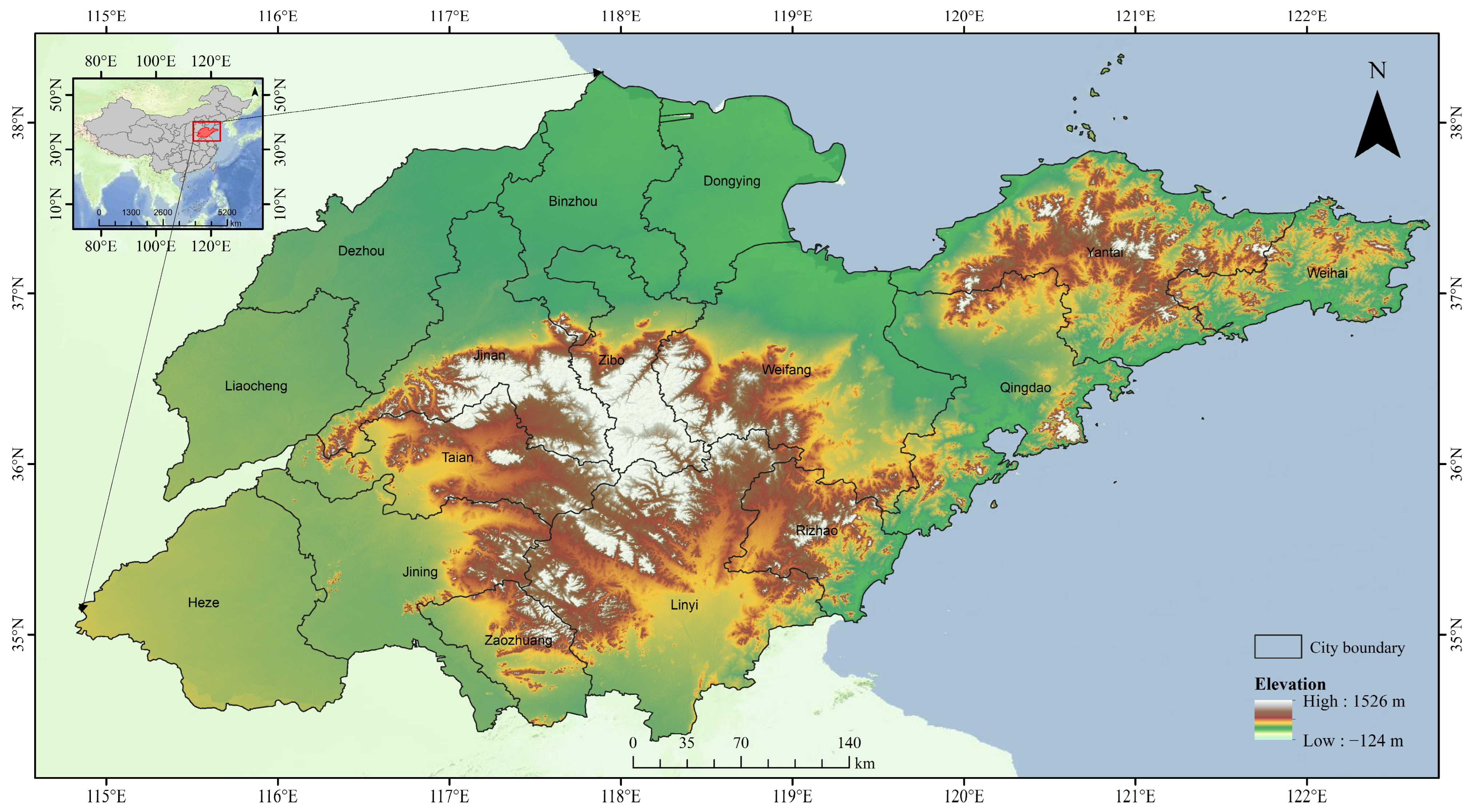
The study area is Shandong Province, which is situated in eastern China along the lower Yellow River (about 34–38°N, 114–122°E). The province experiences a warm temperate monsoon climate characterized by marked seasonal variation, including cold, dry winters and hot, wet summers. Mean annual precipitation ranges from about 500 to 700 mm and falls predominantly during summer, creating suitable moisture and heat conditions for winter wheat cultivation. Owing to these climatic conditions, Shandong is recognized as one of the principal winter wheat-producing provinces in China.

Topographically, plains account for most of the province, while mountainous landforms are concentrated in the central region and hilly areas occur in the east. The northwestern, central, and southwestern plains constitute the principal winter wheat-growing zones, where cultivation is facilitated by relatively complete agricultural infrastructure and suitable irrigation systems.

To support growth-stage-based analysis, the growth-stage windows in this study were defined according to local agricultural calendars, field knowledge, and Sentinel-2 time-series observations. These windows provide a consistent temporal framework for province-wide winter wheat mapping, while local phenological differences may still exist across Shandong Province. The geographic position and spatial coverage of the study area are presented in Figure 1.

2.1.2. Data Acquisition and Preprocessing

The remote sensing data employed in this study were acquired from Sentinel-2 satellites and processed using the Google Earth Engine (GEE) platform. The Sentinel-2 imagery was accessed on 3 May 2025. The Sentinel-2 program consists of Sentinel-2A and Sentinel-2B, offering 13 spectral bands with spatial resolutions of 10 m, 20 m, and 60 m, which are appropriate for crop monitoring and vegetation analysis. The revisit interval of a single satellite is 10 days, whereas the joint operation of the two satellites enables observations every 5 days and thus meets the requirement for multi-temporal data collection.

To maintain the reliability of the dataset, atmospherically corrected Level-2A products were adopted. The image acquisition period extended from October 2023 to June 2024 and covered the entire growth cycle of winter wheat. The growth-stage windows were defined according to the winter wheat agricultural calendar in Shandong Province and local field knowledge. A unified set of windows was used to ensure consistent feature extraction and model comparison across the province. Because each window covered a period rather than a single date, the approach could partially accommodate local differences in phenological timing. At each of the eight growth stages, several Sentinel-2 scenes were chosen, and a median composite was produced to represent that stage. The analysis mainly used the blue (B2), green (B3), red (B4), and near-infrared (B8) bands, all of which were resampled to a spatial resolution of 10 m. The red-edge bands (B5, B6, and B7) together with the shortwave infrared band (B11) were also incorporated for spectral index calculation. Before spectral index calculation, Sentinel-2 Level-2A surface reflectance values were scaled by a factor of 0.0001 to convert the original integer values to reflectance values in the range of 0–1. All spectral indices were calculated using these scaled reflectance values.

During preprocessing, Sentinel-2 images with scene-level cloud cover below 20% were first selected and clipped to the study area boundary in GEE. Median compositing was then performed for each growth-stage window to generate representative images and reduce the influence of residual clouds, cloud shadows, and outliers. Samples with missing spectral index values after compositing were excluded from subsequent feature extraction. The number and distribution of the selected images are shown in Table 1.

2.1.3. Construction of Spectral Variables

Based on Sentinel-2 multispectral imagery, eight spectral variables were extracted across the eight winter wheat growth stages from sowing to maturity: NDVI, EVI, SAVI, GNDVI, NDPI, PSRI, BSI, and B8 (near-infrared reflectance). These variables were used to characterize spectral responses at different growth stages. NDVI, GNDVI, and EVI mainly reflect canopy greenness and crop vigor. SAVI introduces a soil adjustment factor to reduce soil background effects and is therefore more suitable for stages with low vegetation cover. BSI and NDPI characterize bare soil and non-vegetation information and provide auxiliary discrimination at stages with strong vegetation–soil contrast. PSRI is sensitive to vegetation senescence and can be used to characterize changes in canopy structure and physiological status during later growth stages. In addition, B8 can directly reflect crop canopy structural characteristics and provides complementary information to vegetation indices. Therefore, the selected spectral variables cover key information on vegetation growth, soil background, and senescence, and serve as basic inputs for classification modeling and for analyzing the importance of spectral variables within each growth stage.

On this basis, the statistical characteristics of spectral variables at each growth stage were extracted for winter wheat and non-winter wheat samples, and their temporal variations across growth stages were compared. This analysis was used to characterize differences in spectral responses between the two land cover types at different growth stages and to support subsequent analysis of discriminative ability across growth stages and multi-stage combination modeling. The spectral variables and their formulas are listed in

Table 2. Spectral variables and their calculation formulas.

Spectral Variable	Formula	Reference
Normalized Difference Vegetation Index (NDVI)	${\displaystyle \frac{NIR-RED}{NIR+RED}}$	[14]
Enhanced Vegetation Index (EVI)	${\displaystyle \frac{2.5(NIR-RED)}{NIR+6RED-7.5BLUE+1}}$	[15]
Soil-Adjusted Vegetation Index (SAVI)	${\displaystyle \frac{(1+L)(NIR-RED)}{NIR+RED+L}}$	[16]
Green Normalized Difference Vegetation Index (GNDVI)	${\displaystyle \frac{NIR-GREEN}{NIR+GREEN}}$	[17]
Normalized Difference Phenology Index (NDPI)	${\displaystyle \frac{NIR-(0.74\times RED+0.26\times SWIR)}{NIR+(0.74\times RED+0.26\times SWIR)}}$	[18]
Plant Senescence Reflectance Index (PSRI)	${\displaystyle \frac{RED-BLUE}{NIR}}$	[19]
Bare Soil Index (BSI)	${\displaystyle \frac{SWIR+RED-NIR-BLUE}{SWIR+RED+NIR+BLUE}}$	[20]
Near-infrared reflectance (B8/NIR)	Original reflectance of the near-infrared band	[21]

NDVI, EVI, and SAVI are commonly used vegetation indices; B8 (NIR) represents the original reflectance of the near-infrared band; L is the soil adjustment factor (commonly set to 0.5), used to suppress the influence of the soil background.

.

2.1.4. Sample Data in Wheat Field

In this study, a sample database was constructed on the GEE platform. Samples were identified by visual interpretation using Google high-resolution satellite base maps and Sentinel-2 multispectral time-series imagery.

Winter wheat samples were mainly identified based on the clear image differences between the vigorous growth stage, characterized by high vegetation cover, and the maturity and harvest stage, characterized by bare-soil features. Spatial texture information from the high-resolution base maps was used as auxiliary evidence to ensure that sample points were located in homogeneous areas near the centers of fields.

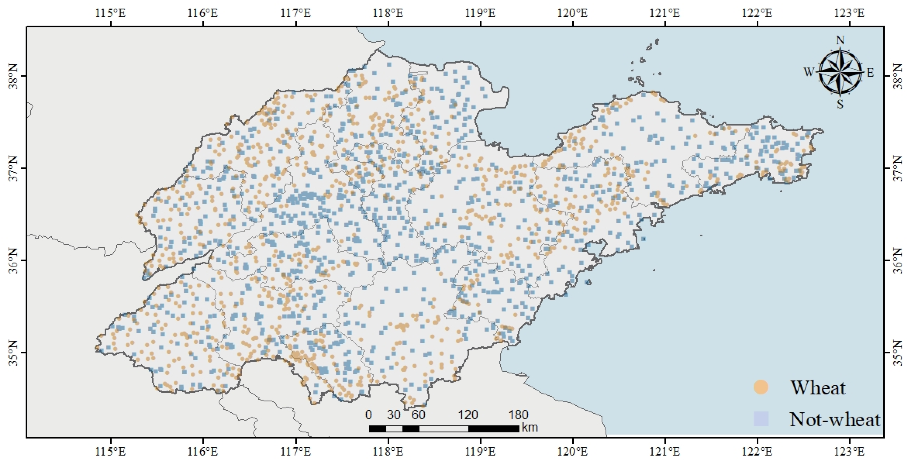
A total of 1015 winter wheat sample points were collected from known winter wheat planting areas across the study region. In addition, 1131 non-winter-wheat sample points were collected, mainly including built-up areas, bare land, water bodies, and other crops, so as to represent heterogeneous non-wheat background conditions. The sample points are discretely distributed across the study area and cover different parts of Shandong Province, helping to represent the spatial distribution of winter wheat and major non-wheat land-cover types. All samples were obtained through manual visual interpretation.

After sample collection, the dataset was randomly divided into a training set and a validation set, with 70% used for model training and 30% used for accuracy validation. After the 70/30 split, the spatial distributions of the training and validation subsets were checked to ensure that both subsets maintained broad spatial coverage across Shandong Province and similar class composition. The spatial distribution of winter wheat and non-winter-wheat sample points in the study area is shown in Figure 2.

2.2. Methods

2.2.1. Technical Framework

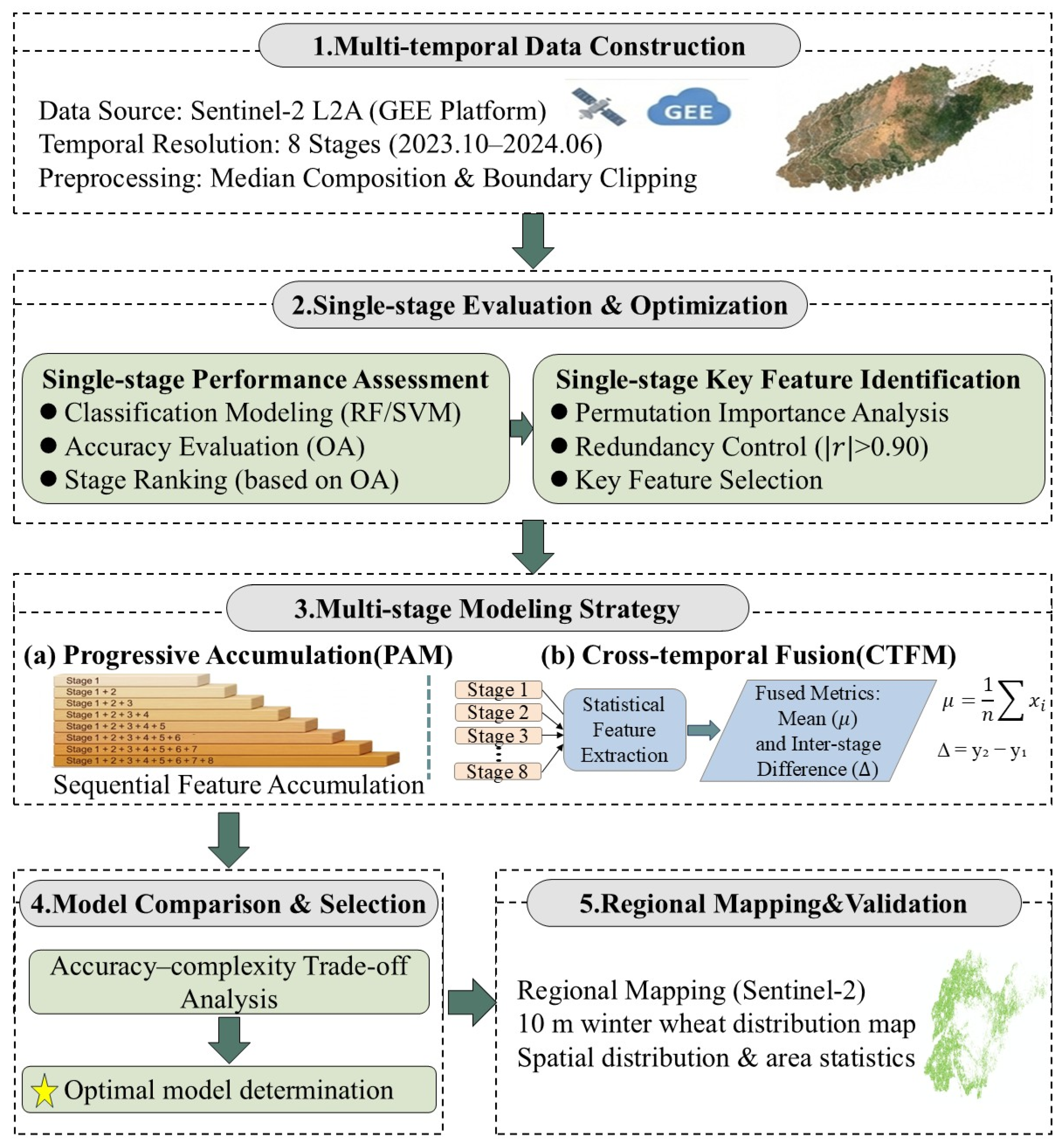
Based on Sentinel-2 multispectral imagery from the 2023–2024 growing season and the phenological characteristics of winter wheat, this study first quantifies the discriminative ability of individual growth stages. A correlation filtering method and permutation importance are then applied to remove redundant variables and select key spectral features.

Next, a progressive accumulation model is constructed by sequentially adding growth stages in descending order of discriminative ability, and the effects of increasing the number of stages on classification accuracy and feature dimensionality are analyzed. For spectral variables that repeatedly appear across multiple stages, a cross-temporal fusion model is further developed by extracting inter-stage mean values and inter-stage differences, enabling a compact representation of multi-stage information.

Finally, the optimal feature combination is applied to Sentinel-2 imagery at the regional scale to produce a winter wheat distribution map at 10 m resolution, followed by analysis of spatial distribution patterns and planting area statistics. The overall technical framework is shown in Figure 3.

2.2.2. Construction and Validation of Single-Stage Identification Models

For the eight growth stages of winter wheat, two supervised classification methods, Support Vector Machine (SVM) and Random Forest (RF), were employed to construct identification models [22,23]. Both models used eight spectral variables—NDVI, EVI, SAVI, GNDVI, NDPI, PSRI, BSI, and B8—as input features, and were evaluated under the same sample conditions and assessment framework.

The SVM used the radial basis function (RBF) kernel, with other hyperparameters kept at their default settings. For the RF model, the number of trees was set to 100 and the maximum tree depth was set to 10, while other hyperparameters were kept at their default settings. Before training, all input features were normalized using Min–Max scaling, and model performance was evaluated using an independent validation dataset.

Model performance was assessed mainly using overall accuracy (OA), F1-score, producer’s accuracy (PA), and user’s accuracy (UA), while the Kappa coefficient was additionally reported as a supplementary metric [24]. OA reflects overall classification accuracy, and Kappa provides an additional measure of agreement beyond chance. Following recent recommendations on classification accuracy assessment, model comparison and selection in this study were mainly based on OA, F1-score, PA, UA, and feature dimensionality [25].

$$OA={\displaystyle \frac{TP+TN}{N}}$$

(1)

$$Kappa={\displaystyle \frac{P_o-P_e}{1-P_e}}$$

(2)

$$P_o={\displaystyle \frac{TP+TN}{N}},P_e={\displaystyle \frac{\left(TP+FP\right)\left(TP+FN\right)+\left(FN+TN\right)\left(FP+TN\right)}{N^2}}$$

(3)

where TP and TN denote correctly classified winter wheat and non-winter-wheat samples, respectively; FP and FN denote misclassified samples; and $N$ is the total number of samples.

In addition, PA and UA represent omission error and classification reliability, respectively, while the F1-score provides a comprehensive evaluation of winter wheat classification performance [26].

To ensure the reliability of subsequent modeling, SVM and RF were compared at each growth stage under identical conditions. The classifier with superior and more stable performance, mainly judged by OA and F1-score, was then selected for the progressive accumulation model and the cross-temporal fusion model, thereby avoiding the propagation of suboptimal classification performance in later modeling stages. Meanwhile, the eight growth stages were ranked according to the overall accuracy of the single-stage models to quantify their discriminative ability.

2.2.3. Key Spectral Variable Selection

At the single-growth-stage level, the importance of spectral variables was evaluated using the Random Forest (RF) model. For each of the eight growth stages, independent RF classification models were constructed (with parameter settings consistent with Section 2.2.2), using eight spectral variables—NDVI, EVI, SAVI, GNDVI, NDPI, PSRI, BSI, and B8—as input features.

To reduce multicollinearity among spectral variables, a correlation-based filtering strategy was introduced. Pearson correlation coefficients among the spectral variables within each growth stage were first calculated:

$$r={\displaystyle \frac{{\displaystyle {\sum }_{i=1}^n}(x_i-\stackrel{-}{x}\left)\right(y_i-\stackrel{-}{y})}{\sqrt{{\displaystyle {\sum }_{i=1}^n}(x_i-\stackrel{-}{x}{)}^2{\displaystyle {\sum }_{i=1}^n}(y_i-\stackrel{-}{y}{)}^2}}}$$

(4)

Variables with an absolute Pearson correlation coefficient greater than 0.90 were considered highly correlated, following previous correlation-based covariate filtering practices in remote-sensing studies [27]. Permutation importance was then used to quantify the contribution of each spectral variable. This method evaluates the change in model performance after randomly permuting a given variable in the validation dataset while keeping the model unchanged. A larger decrease in performance indicates higher importance of the variable. The permutation importance is defined as:

$$I_j={\displaystyle \frac{1}{R}}{\displaystyle \sum _{r=1}^R}\left[S\left(D_{val}\right)-S\left({\pi }_j^{\left(r\right)}\left(D_{val}\right)\right)\right]$$

(5)

where $I_j$ is the importance of the $j$-th variable, $S(\cdot )$ denotes the evaluation metric (overall accuracy, OA, in this study), $D_{val}$ is the validation dataset, ${\pi }_j^{\left(r\right)}(\cdot )$ represents the dataset after permuting the $j$-th variable in the $r$-th iteration, and $R$ is the number of permutations.

The spectral variables were first ranked in descending order of permutation importance. To further reduce redundancy, the correlation constraint was applied: if the absolute correlation between a candidate variable and the retained variables exceeded 0.90, the variable was considered redundant and discarded, and only the variable with higher importance was retained.

To facilitate comparison within each growth stage, the mean importance of all remaining variables was used as a threshold:

$$\stackrel{-}{I}={\displaystyle \frac{1}{m}}{\displaystyle \sum _{j=1}^m}{I}_j$$

(6)

where $m$ is the number of variables after redundancy removal. Variables satisfying $I_j\ge \stackrel{-}{I}$ were selected as key spectral variables for that growth stage. These selected variables were used as input features for subsequent construction of the progressive accumulation model and the cross-temporal fusion model.

2.2.4. Multi-Stage Model Construction and Validation

Based on the key spectral variables selected for each growth stage, two multi-stage feature construction strategies were developed: a progressive accumulation model (PAM) and a cross-temporal fusion model (CTFM). Both strategies were evaluated using the same classifier and parameter settings as the single-stage models to ensure comparability.

In the PAM, the eight growth stages were first ranked according to the overall accuracy (OA) of the single-stage models. Multi-stage information was then progressively accumulated following this ranking to construct models $M_1$–$M_8$. Specifically, model $M_n$ incorporates the key spectral variables from the top $n$ growth stages ranked by discriminative ability. Spectral variables with the same name but from different growth stages were treated as distinct features to preserve stage-specific information.

In the CTFM, spectral variables that appeared in multiple growth stages were identified and aggregated. Following the chronological order of growth stages, cross-temporal statistical features were constructed, including inter-stage mean values (mean) and inter-stage differences (diff), where the difference was defined as the value at the last included growth stage minus that at the first included growth stage. For variables available from only one included growth stage, the same feature-construction framework was retained, with the difference term contributing no additional temporal variation. These features represent the overall spectral level and the cumulative temporal change, respectively. Corresponding fusion models $M_1$–$M_8$ were then developed.

It should be noted that growth stages were ranked by discriminative ability for PAM construction, while chronological order was used for cross-temporal feature computation in CTFM.

To evaluate model performance and feature efficiency, a unified set of training and validation samples was used for both strategies. Classification performance was assessed using overall accuracy (OA), F1-score, producer’s accuracy (PA), and user’s accuracy (UA), while the Kappa coefficient was also reported as a supplementary metric. Combined with feature dimensionality, the trade-off between classification accuracy and model complexity was systematically analyzed. In addition, a full-stacked RF baseline was constructed by directly stacking all eight spectral variables from the eight growth stages, resulting in 64 temporal–spectral features. This baseline was used to evaluate whether the proposed feature selection and fusion strategies could maintain comparable accuracy while reducing feature dimensionality. To further compare the proposed framework with a representative deep learning temporal classification method, a one-dimensional convolutional neural network (1D-CNN), which is a commonly used Temporal CNN architecture for sequence classification, was constructed using the complete 8 × 8 temporal–spectral feature matrix. The eight growth stages were arranged according to the chronological order of winter wheat development, and the eight spectral variables at each stage were used as input channels. The 1D-CNN was evaluated using the same five-fold cross-validation strategy and accuracy metrics as the RF-based models. The 1D-CNN consisted of two one-dimensional convolutional layers with 32 and 64 filters, respectively, followed by batch normalization, max-pooling, a fully connected layer with 64 neurons, dropout, and a sigmoid output layer. The model was trained using the Adam optimizer and early stopping.

Finally, the optimal model was determined by jointly considering classification accuracy, feature dimensionality, and cross-validation stability. Its performance was further validated at the regional scale through spatial distribution analysis, provincial-level area error assessment, and consistency evaluation with municipal-level statistical data. At the municipal scale, regression analysis between remotely sensed estimates and statistical yearbook data was conducted, and model performance was quantified using the coefficient of determination ($R^2$).

3. Results

3.1. Temporal Variation in Spectral Variables Across Growth Stages

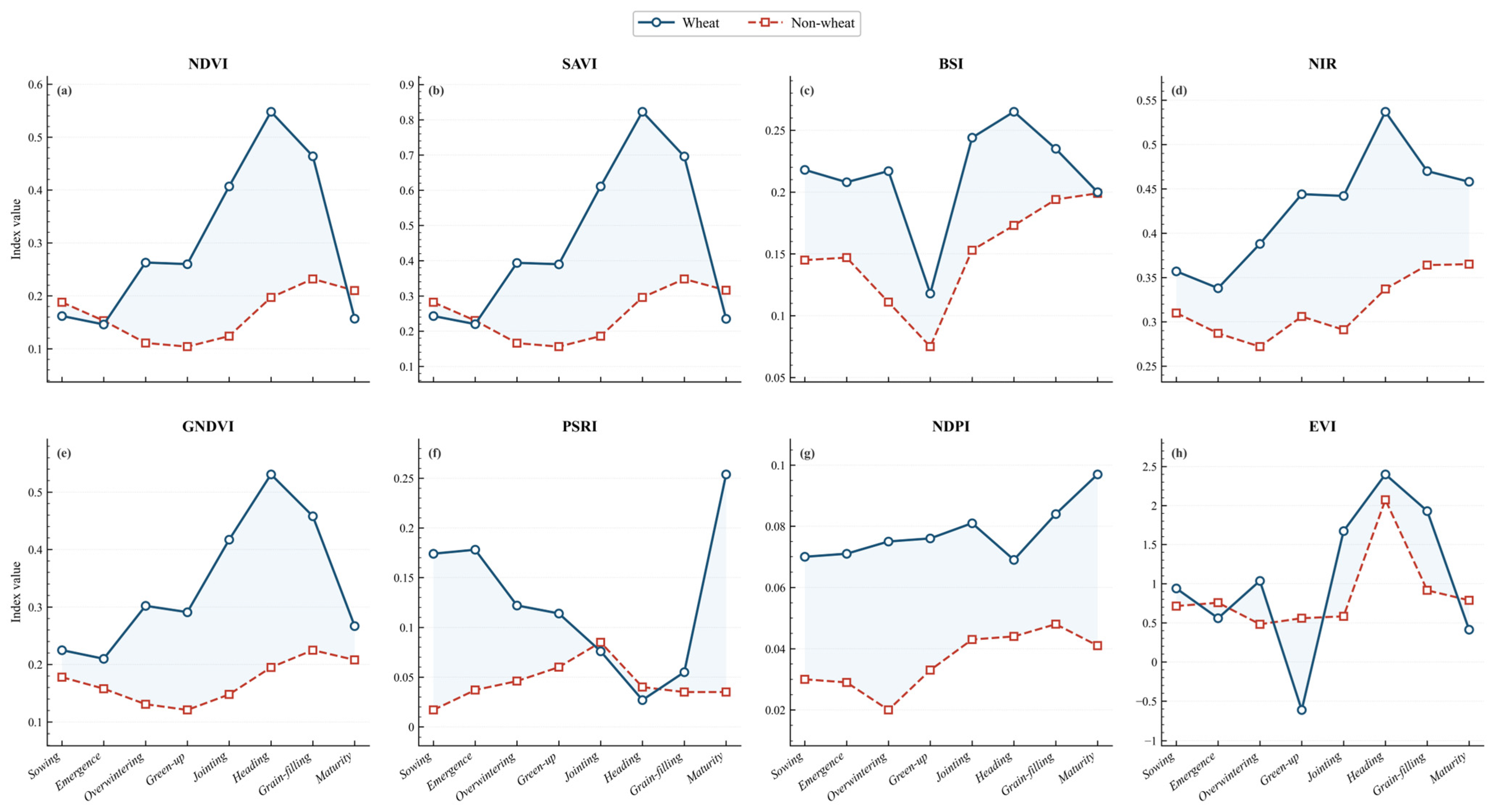
The temporal variations in winter wheat and non-wheat samples across eight spectral variables (NDVI, SAVI, BSI, NIR (B8), GNDVI, PSRI, NDPI, and EVI) over different growth stages are shown in Figure 4.

Overall, non-wheat samples exhibit consistently low values in vegetation-related variables (NDVI, SAVI, and GNDVI) from the overwintering to grain-filling stages, with relatively limited variation across stages. In contrast, winter wheat samples show pronounced stage-dependent patterns along the growth cycle. NDVI, SAVI, and GNDVI gradually increase from the overwintering stage, peak during the jointing–heading stages, remain relatively high during the heading–grain-filling stages, and decline sharply at maturity. EVI increases rapidly from the jointing stage, reaches its maximum at heading, and then decreases toward maturity. Similarly, NIR (B8) shows an increasing trend from the emergence stage, peaks at heading, and declines thereafter. In contrast, BSI exhibits relatively low values during the green-up stage but increases during the jointing–grain-filling stages. PSRI and NDPI show clear increasing trends from the grain-filling stage to maturity, with PSRI exhibiting a particularly sharp increase at the maturity stage.

Inter-class comparisons reveal distinct spectral differences between winter wheat and non-wheat samples across most growth stages. These differences are especially pronounced for NDVI, SAVI, GNDVI, and NIR (B8) during the jointing–heading stages, and remain evident during the grain-filling stage. At the maturity stage, PSRI shows the strongest discriminative ability between the two classes. These results highlight the stage-dependent discriminative potential of spectral variables and provide a basis for subsequent stage ranking and key variable selection.

3.2. Single-Stage Identification of Winter Wheat

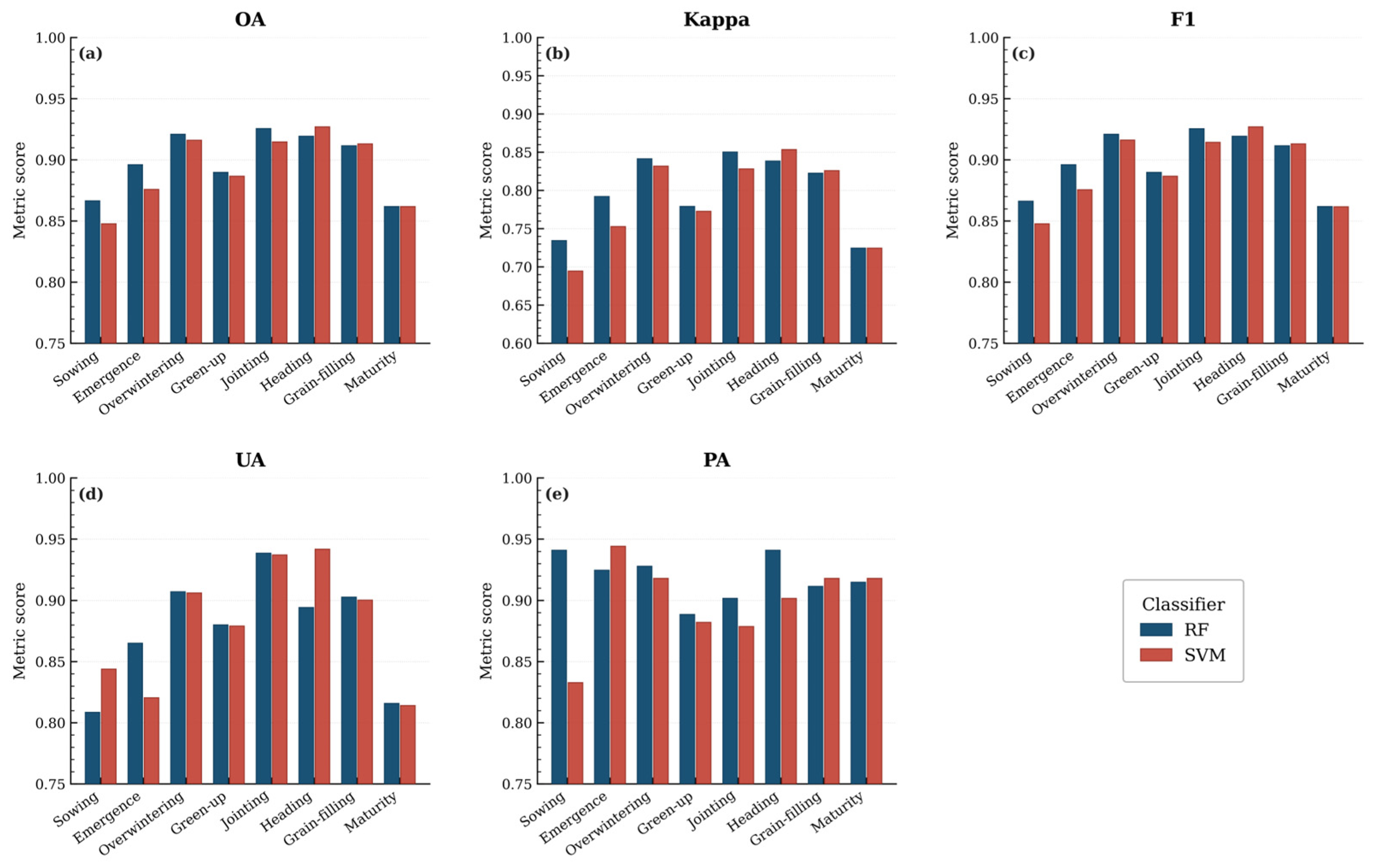
To ensure a reliable evaluation of discriminative ability across growth stages, the classification performance of Support Vector Machine (SVM) and Random Forest (RF) was first compared across the eight growth stages (Figure 5). Overall, RF slightly outperformed SVM in most stages, mainly in terms of OA and F1-score, while Kappa showed a similar supplementary trend. The average F1-scores were 0.8989 for RF and 0.8928 for SVM, while the average Kappa coefficients were 0.7978 and 0.7855, respectively. Although SVM showed advantages in some individual cases, RF demonstrated slightly better overall performance and more consistent results across growth stages, and was therefore selected for subsequent analysis.

Under the RF framework, winter wheat identification accuracy varied significantly across growth stages. Based on OA from independent validation samples, the stages ranked in descending order were: jointing (0.9255), overwintering (0.9208), heading (0.9193), grain-filling (0.9115), emergence (0.8960), green-up (0.8898), sowing (0.8680), and maturity (0.8618). The jointing, overwintering, and heading stages achieved the highest accuracy, indicating strong discriminative ability, whereas the sowing and maturity stages showed a weaker performance.

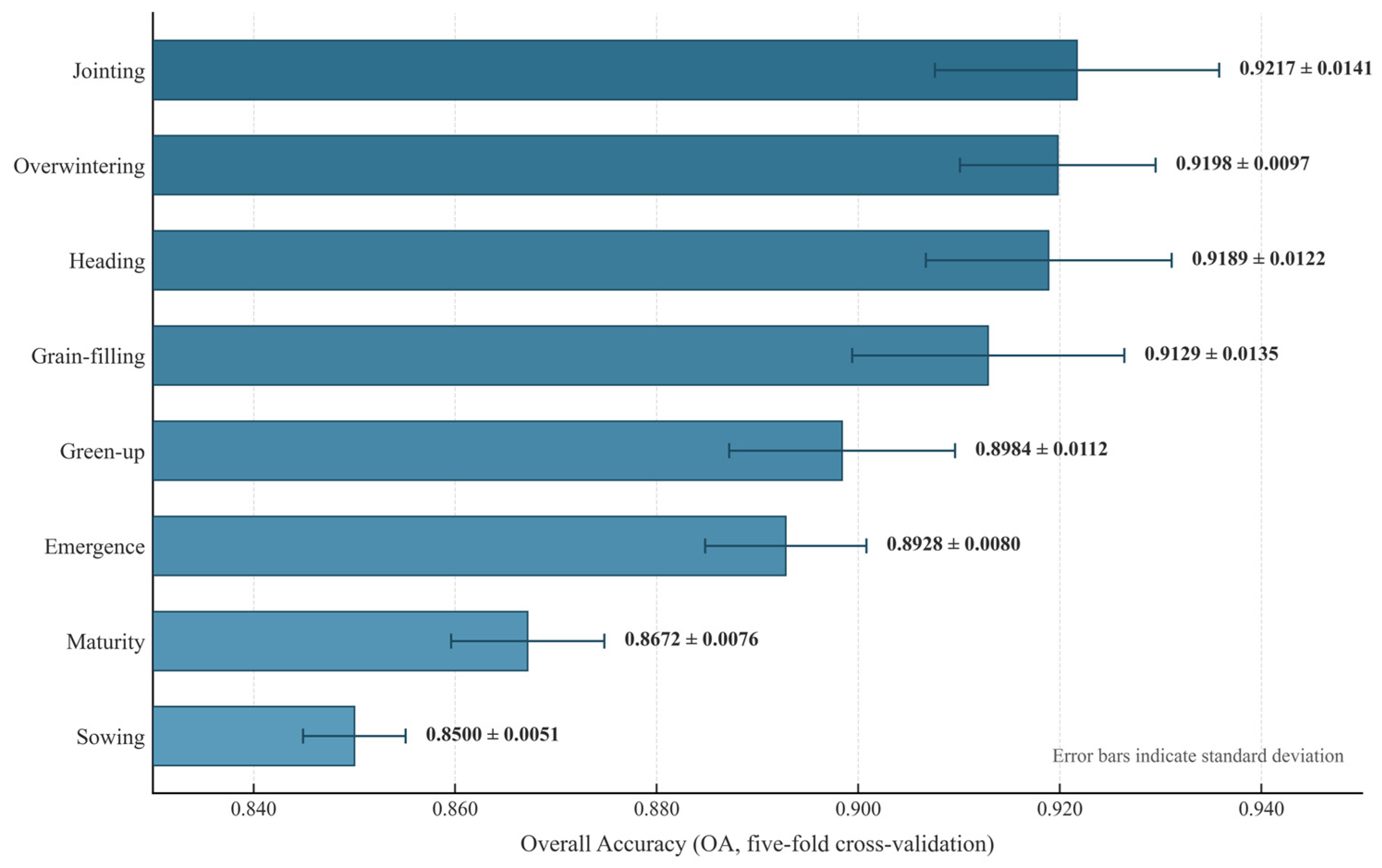
To further evaluate the stability of single-stage classification performance under different sample partitions, five-fold cross-validation was conducted for the RF models (Figure 6). The cross-validation results showed a pattern generally consistent with the independent validation results. The jointing, overwintering, heading, and grain-filling stages maintained relatively high OA values of 0.9217 ± 0.0141, 0.9198 ± 0.0097, 0.9189 ± 0.0122, and 0.9129 ± 0.0135, respectively. In contrast, the sowing and maturity stages showed lower OA values of 0.8500 ± 0.0051 and 0.8672 ± 0.0076, respectively. These results indicate that the ranking of growth-stage discriminative ability was generally stable under different sample partitions.

These results indicate that the most informative stages for winter wheat identification are concentrated in the jointing, overwintering, heading, and grain-filling stages, while the sowing and maturity stages contribute less discriminative information. This stage-dependent variability provides a basis for subsequent stage ranking and model construction in the progressive accumulation model (PAM) and the cross-temporal fusion model (CTFM).

3.3. Key Spectral Variables Across Growth Stages

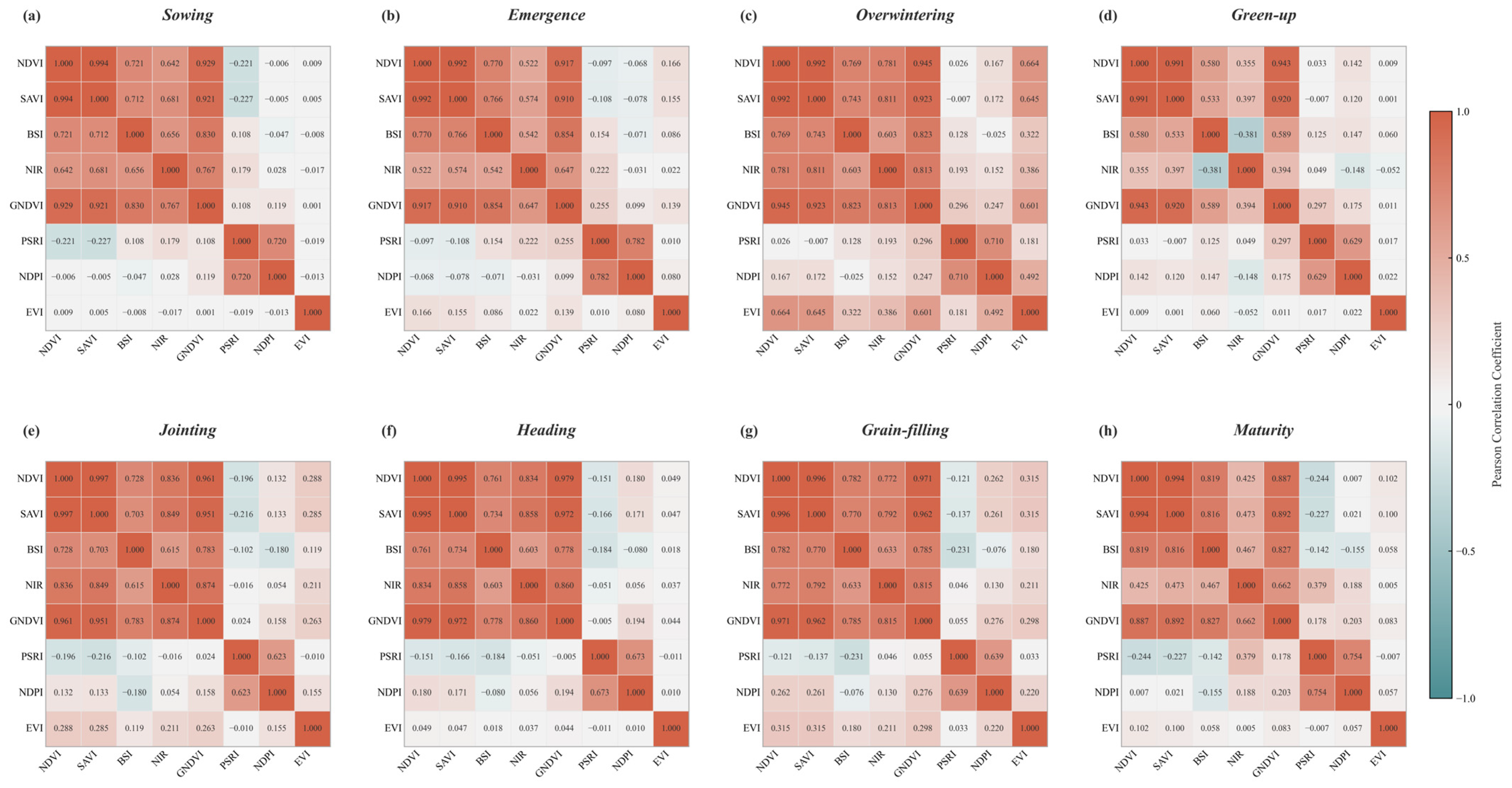
As shown in Figure 7, strong correlations were observed among multiple spectral variables across different growth stages. NDVI and SAVI exhibited extremely high positive correlations throughout all stages ($r\ge 0.991$). NDVI and GNDVI also showed strong positive correlations, particularly at the heading ($r=0.979$) and grain-filling ($r=0.971$) stages. In addition, PSRI and NDPI maintained consistent positive correlations across all stages ($r=0.623–0.782$). These results indicate clear correlation clustering among vegetation-related indices within individual growth stages.

However, the correlation structure varied across growth stages. For example, the correlation between EVI and NDVI was 0.664 at the overwintering stage but decreased to 0.009 at the green-up stage. Similarly, NIR and BSI were negatively correlated at the green-up stage ($r=-0.381$) but positively correlated at the sowing stage ($r=0.656$). These variations suggest that inter-variable relationships are stage-dependent.

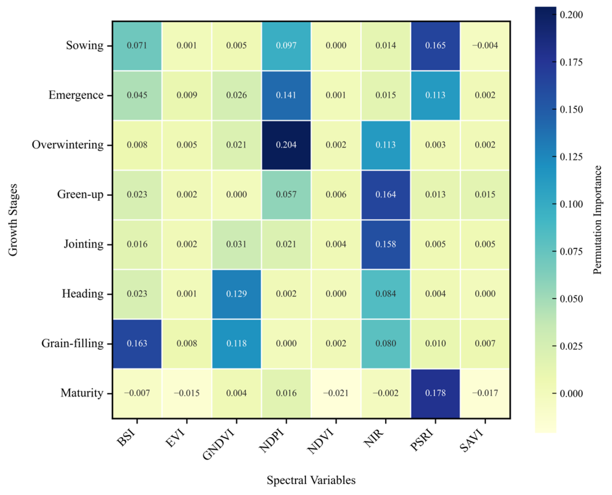
Based on these patterns, permutation importance was applied to evaluate the contribution of spectral variables in single-growth-stage RF models, combined with a correlation threshold ($\mid r\mid >0.90$) to reduce redundancy. This strategy enables the identification of key variables with strong complementary information.

The distribution of permutation importance values for each growth stage is shown in Figure 8. Using the mean importance as a threshold, variables with above-average importance were retained, and further filtered using the correlation constraint. As shown in

Table 3. Selection results of key spectral variables for different growth stages.

Growth Stage	No. of Key Spectral Variables	Key Spectral Variables
Sowing Stage	3	PSRI, NDPI, BSI
Emergence Stage	2	NDPI, PSRI
Overwintering Stage	2	NDPI, NIR
Green-up Stage	2	NIR, NDPI
Jointing Stage	1	NIR
Heading Stage	2	GNDVI, NIR
Grain-filling Stage	3	BSI, GNDVI, NIR
Maturity Stage	1	PSRI

, the number of variables was reduced from eight to one–three per stage.

Specifically, PSRI, NDPI, and BSI were selected during the sowing stage, while NDPI and PSRI were retained during the emergence stage. NDPI and NIR were retained during the overwintering and green-up stages, while GNDVI and NIR were selected during the heading stage. In contrast, only a single dominant feature was retained for the jointing and maturity stages, namely NIR and PSRI, respectively. Notably, variables such as NDPI and PSRI appeared repeatedly across multiple stages, indicating consistent representational capability for winter wheat across growth stages.

After feature selection, the original 64-dimensional feature space (eight stages × eight variables) was reduced to 16 dimensions. To examine the sensitivity of the correlation threshold, additional tests were conducted using alternative thresholds of $\mid r\mid$ > 0.85 and $\mid r\mid$ > 0.95. The total number of selected stage-specific variables changed only slightly from 15 to 17, compared with 16 under the $\mid r\mid$ > 0.90 threshold. However, the set of unique selected spectral variables remained unchanged, including BSI, GNDVI, NDPI, NIR, and PSRI. This indicates that the key variable selection results were not highly sensitive to the specific correlation threshold, and suggests that $\mid r\mid$ > 0.90 provided a practical balance between redundancy reduction and information preservation. Overall, this feature selection strategy effectively mitigates multicollinearity while preserving key discriminative information, providing compact and efficient inputs for the subsequent progressive accumulation model (PAM) and cross-temporal fusion model (CTFM).

3.4. Multi-Stage Identification Models: Accumulation vs. Fusion

Based on the key spectral variables selected for each growth stage, two multi-stage models were constructed: the progressive accumulation model (PAM) and the cross-temporal fusion model (CTFM). Their classification performance is shown in

Table 4. Classification Performance of the Progressive Accumulation Model (PAM) and the Cross-Temporal Fusion Model (CTFM).

Type	Model	Added Growth Stage	Dim	OA	Kappa	F1	PA	UA
PAM	M1	Jointing	1	0.8354	0.6704	0.8355	0.8426	0.8159
	M2	+Overwintering	3	0.9193	0.8383	0.9193	0.9311	0.9016
	M3	+Heading	5	0.9425	0.8848	0.9425	0.9377	0.9408
	M4	+Grain-filling	8	0.9503	0.9004	0.9503	0.9508	0.9446
	M5	+Emergence	10	0.9627	0.9253	0.9627	0.9705	0.9518
	M6	+Green-up	12	0.9674	0.9347	0.9674	0.9770	0.9551
	M7	+Sowing	15	0.9689	0.9378	0.9690	0.9770	0.9582
	M8	+Maturity	16	0.9689	0.9378	0.9690	0.9770	0.9582
CTFM	M1	Jointing	2	0.8354	0.6704	0.8355	0.8426	0.8159
	M2	+Overwintering	4	0.9270	0.8540	0.9271	0.9475	0.9031
	M3	+Heading	6	0.9363	0.8723	0.9363	0.9344	0.9314
	M4	+Grain-filling	8	0.9410	0.8817	0.9410	0.9377	0.9377
	M5	+Emergence	10	0.9643	0.9284	0.9643	0.9705	0.9548
	M6	+Green-up	10	0.9658	0.9315	0.9658	0.9672	0.9609
	M7	+Sowing	10	0.9643	0.9284	0.9643	0.9607	0.9638
	M8	+Maturity	10	0.9627	0.9253	0.9627	0.9672	0.9547

PAM and CTFM denote the progressive accumulation model and cross-temporal fusion model, respectively. “+” indicates the incremental addition of growth stages based on the previous model. PA and UA denote Producer’s Accuracy and User’s Accuracy, respectively.

.

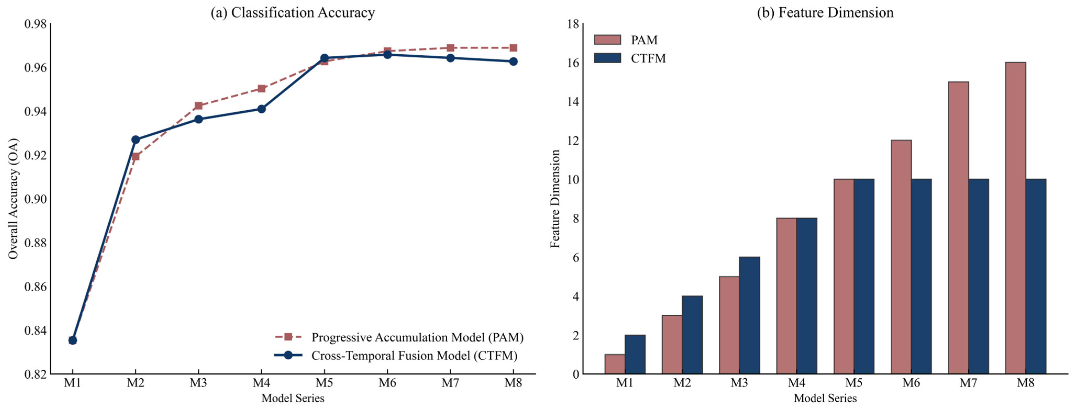
As growth-stage information was progressively incorporated, both models showed overall improvements in the primary accuracy metrics, especially OA and F1-score, although the magnitude and pattern of improvement differed. The performance trends and feature-dimensionality changes are further illustrated in Figure 9.

For the PAM, feature dimensions increase from 1 (M1) to 16 (M8) through sequential accumulation of stage-specific features. Model performance improves steadily, reaching a maximum OA of 0.9689 at M7 (15 dimensions), with no further improvement at M8. This indicates that simply adding features from later growth stages provides limited additional benefit and may introduce redundancy.

In contrast, the CTFM constructs features by integrating inter-stage mean and difference (diff) characteristics of key spectral variables. Feature dimensionality stabilizes at 10 after M5. The OA reaches 0.9643 at M5 and slightly increases to 0.9658 at M6, after which no further sustained improvement is observed. Compared with PAM, CTFM achieves stable performance at intermediate stages without increasing feature dimensionality.

Comparative analysis shows that PAM achieves the highest OA (0.9689) but requires 15–16 feature dimensions. In contrast, CTFM achieves comparable accuracy (OA = 0.9658) using only 10 dimensions and attains a relatively high user’s accuracy (UA = 0.9609) at M6. Considering the trade-off between accuracy improvement and feature dimensionality, CTFM demonstrates superior efficiency in feature utilization.

To further evaluate model stability and provide baseline comparisons, five-fold cross-validation was conducted for representative models, including the full-stacked RF model using all 64 original temporal–spectral features, PAM M7, CTFM M6, and a 1D-CNN temporal classification baseline (

Table 5. Five-fold cross-validation results of representative multi-stage and deep-learning baseline models.

Model	Dim	OA	Kappa	F1	PA	UA
Full-stacked RF	64	0.9716 ± 0.0078	0.9430 ± 0.0157	0.9700 ± 0.0085	0.9744 ± 0.0182	0.9660 ± 0.0097
PAM M7	15	0.9660 ± 0.0042	0.9319 ± 0.0084	0.9645 ± 0.0042	0.9764 ± 0.0088	0.9531 ± 0.0114
CTFM M6	10	0.9613 ± 0.0094	0.9225 ± 0.0189	0.9593 ± 0.0189	0.9635 ± 0.0205	0.9554 ± 0.0157
1D-CNN	8 × 8	0.9078 ± 0.0486	0.8131 ± 0.0992	0.8917 ± 0.0612	0.8296 ± 0.1113	0.9720 ± 0.0132

Full-stacked RF denotes the baseline model constructed by directly stacking all 64 temporal–spectral features. PAM M7 and CTFM M6 denote the best-performing progressive accumulation model and the selected cross-temporal fusion model, respectively. The 1D-CNN denotes the representative Temporal CNN baseline constructed using the complete 8 × 8 temporal–spectral feature matrix. Values are reported as mean ± standard deviation.

). The full-stacked RF model served as a baseline representing direct multi-temporal feature stacking without feature selection or fusion, while the 1D-CNN was used as a representative deep-learning temporal baseline.

To complement the summary accuracy metrics, confusion matrices of the representative multi-stage and deep-learning baseline models were calculated from the out-of-fold predictions of five-fold cross-validation (

Table 6. Confusion matrices of representative multi-stage and deep-learning baseline models based on out-of-fold predictions from five-fold cross-validation.

Model	Correct Wheat	Wheat Missed	Non-Wheat Misclassified as Wheat	Correct Non-Wheat
Full-stacked RF	989	26	35	1096
PAM M7	991	24	49	1082
CTFM M6	978	37	46	1085
1D-CNN	842	173	25	1106

Values were obtained by aggregating out-of-fold predictions across the five folds; therefore, each of the 2146 samples was predicted once. Wheat and non-wheat denote winter wheat and non-winter-wheat samples, respectively.

).

The full-stacked RF model achieved the highest OA of 0.9716 ± 0.0078 and showed the fewest total misclassified samples in the cross-validation confusion matrix, but required 64 input features. In comparison, CTFM M6 achieved an OA of 0.9613 ± 0.0094 and an F1-score of 0.9593 ± 0.0189 using only 10 fused features, reducing the feature dimensionality by 84.4% relative to the full-stacked baseline. The 1D-CNN baseline achieved an OA of 0.9078 ± 0.0486 and an F1-score of 0.8917 ± 0.0612, which were lower than those of the RF-based multi-stage models. In addition, the relatively larger standard deviations indicate that the 1D-CNN was less stable under the current sample size and feature setting. Although CTFM M6 was slightly less accurate than the full-stacked RF and PAM M7 models, it provided a compact representation of multi-stage information with stable cross-validation performance, supporting its selection as the optimal model when both accuracy and feature efficiency were considered.

Therefore, considering classification accuracy, cross-validation stability, and feature dimensionality, CTFM M6 was selected as the optimal model for subsequent winter wheat mapping. This model incorporates cross-temporal mean and difference features of key spectral variables from six growth stages—jointing, overwintering, heading, grain-filling, emergence, and green-up—resulting in a compact feature set of 10 variables.

3.5. Model Application and Winter Wheat Mapping in Shandong Province

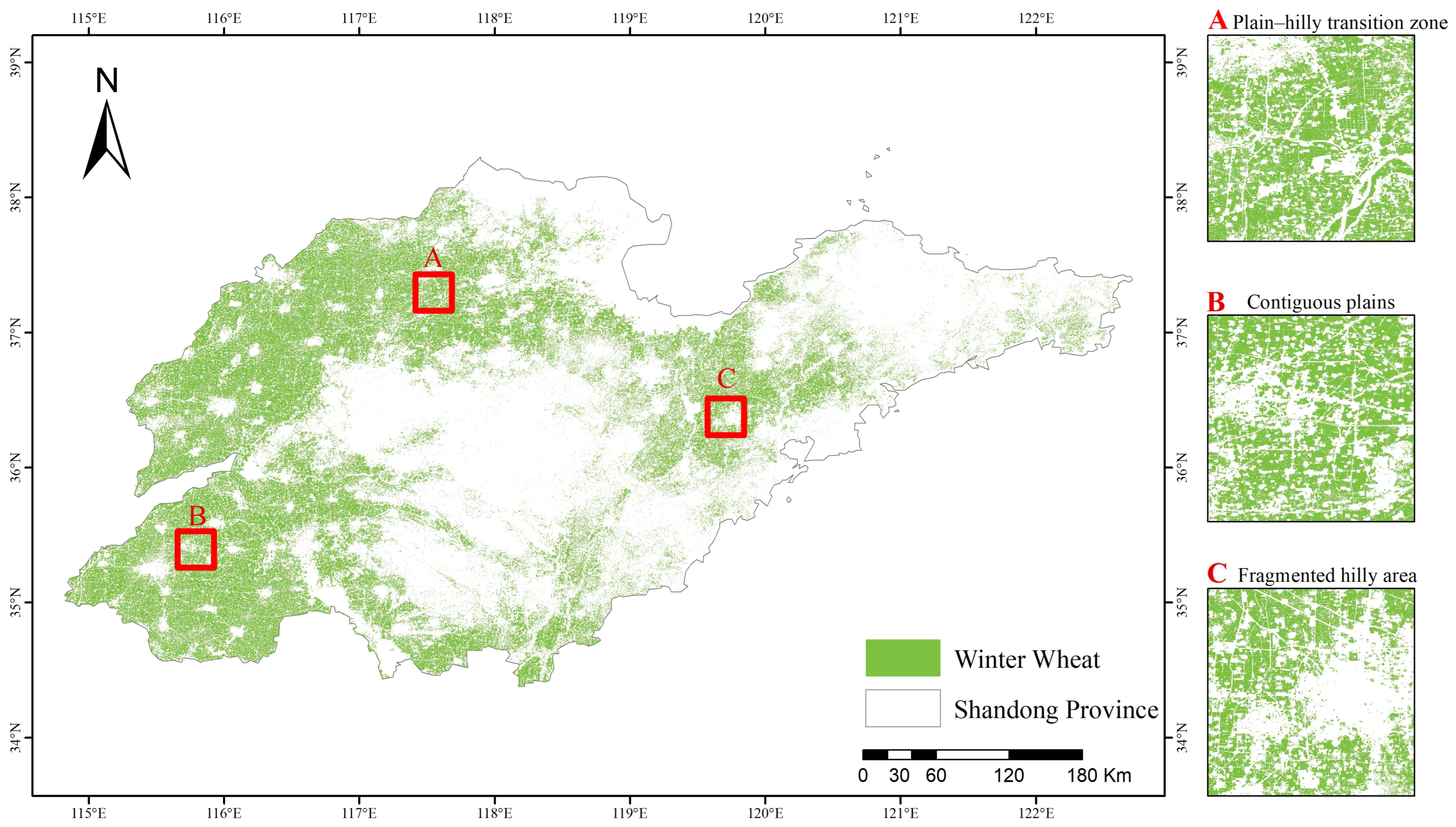
Based on the above analysis of the progressive accumulation model and the cross-temporal fusion model, the cross-temporal fusion model (CTFM) M6 was selected as the optimal model to map winter wheat distribution across Shandong Province using Sentinel-2 imagery from the 2023–2024 growing season. This model employs a Random Forest classifier and uses fused features derived from key spectral variables, including inter-stage mean values (mean) and inter-stage differences (diff), resulting in a total of 10 input features. Based on this model, a winter wheat distribution map with a spatial resolution of 10 m was generated (Figure 10).

As shown in Figure 10, winter wheat is mainly distributed in southwestern Shandong, the northwestern Shandong Plain, and central Shandong, forming large, contiguous planting areas. In contrast, the distribution is more fragmented in mountainous regions of central and eastern Shandong. The overall spatial pattern is consistent with the known geographic distribution of major winter wheat production areas, indicating that the CTFM effectively captures regional-scale distribution characteristics.

To further evaluate spatial performance, three representative regions (A–C) were selected for local analysis, corresponding to the plain–hilly transition zone, contiguous plains, and fragmented hilly areas, respectively. Region B (contiguous plains) shows high spatial continuity and clear field boundaries, whereas Region C (fragmented hilly area) exhibits scattered patches and limited misclassification, likely due to terrain complexity and fragmented cropland structure.

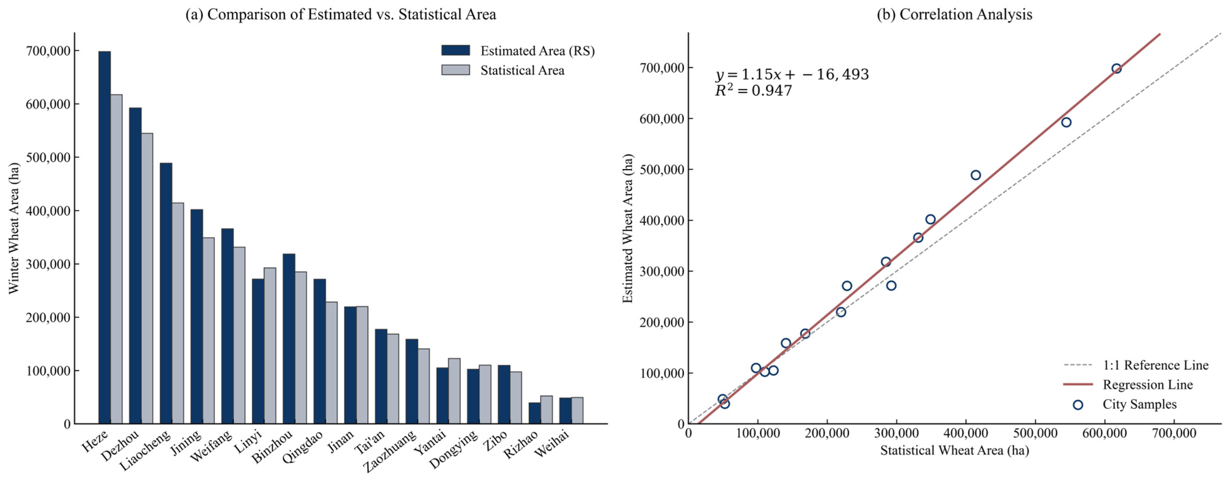
At the provincial scale, the relative error between the remotely sensed estimated winter wheat area and statistical yearbook data was 8.55%. At the municipal scale, Figure 11a shows that the spatial distribution of estimated areas is generally consistent with statistical data, with higher values observed in major producing regions and slight underestimation in some non-major producing areas. Furthermore, Figure 11b demonstrates a strong linear relationship between remotely sensed estimates and statistical data (R² = 0.947), with a regression slope of 1.15. The RMSE, MAE, and MAPE were 37,739 ha, 29,137 ha, and 11.38%, respectively, providing additional quantitative measures of municipal-level estimation error.

4. Discussion

4.1. Differences in Identification Performance Among Growth Stages

The results of this study indicate that remote sensing-based winter wheat identification performance differs significantly across growth stages. Among them, the jointing stage showed the strongest discriminative ability, with an OA of 0.9255 and a high F1-score. This result is closely related to the physiological characteristics of the jointing stage. As a key period in the transition from vegetative to reproductive growth, the jointing stage is characterized by rapid increases in leaf area index and vegetation cover, enabling winter wheat to form stable and distinct spectral differences from non-wheat land cover types in the near-infrared band and vegetation indices such as NDVI, GNDVI, and SAVI. This provides a strong basis for remote sensing identification. These findings are consistent with previous studies. For example, Liu et al. (2022), based on Sentinel-2 time-series imagery, reported that the jointing-to-heading stage is the period with the highest winter wheat identification accuracy, with an overall accuracy of up to 96.90% [28].

The overwintering stage also shows relatively high identification accuracy (OA = 0.9208). Although winter wheat biomass remains low at this stage, it still maintains a certain level of vegetation cover compared with bare land, forming stable distinctions from non-wheat land cover types in variables such as NDPI and near-infrared reflectance. This conclusion is also supported by previous studies. Liu et al. (2023) reported that NDPI during the overwintering stage can effectively suppress interference from soil and snow backgrounds, thereby enhancing weak vegetation signals [29]. Dong et al. (2020) likewise found that the relative stability of vegetation cover during the overwintering stage improves the reliability of regional-scale winter wheat identification in North China [30].

The identification accuracy during the heading and grain-filling stages is slightly lower than that during the jointing and overwintering stages, but remains relatively high overall. During the heading stage, the winter wheat canopy structure tends to stabilize, and vegetation indices reach or approach their peak values, allowing effective discrimination from other crops and non-crop land cover types. Although some vegetation indices begin to decline during the grain-filling stage, differences in physiological status and spectral responses between winter wheat and background land cover types still provide useful discriminative information. Qiu et al. (2017), through EVI2 time-series analysis, showed that vegetation index changes around the heading stage are important for winter wheat identification [31]. Similarly, Lv et al. (2023), in optimizing winter wheat extraction using NDPI time series, identified the jointing–heading stage and the grain-filling-harvest stage as core discriminative periods, which is consistent with the present findings [32].

In contrast, identification performance during the sowing and maturity stages is weak. During the sowing stage, winter wheat has not yet formed continuous vegetation cover, and its spectral characteristics are easily confused with those of bare land and winter fallow fields. Therefore, this stage was not expected to provide strong direct spectral evidence of winter wheat plants. It was included mainly as an early background reference period within the complete phenological sequence, rather than as a core stage for direct winter wheat identification. The weak performance at the sowing stage therefore helps identify the temporal boundary before winter wheat becomes spectrally separable from non-wheat background land cover. This is also consistent with the optimal CTFM M6 model, in which the sowing stage was not retained as one of the core stages. During the maturity stage, plants enter senescence, and declining chlorophyll content reduces vegetation index values, causing spectral responses to become more similar to those of some non-crop land cover types and increasing classification uncertainty. Yang et al. (2023) found in a national-scale study that winter wheat identification accuracy remains relatively low from the sowing stage to the pre-overwintering stage because of low vegetation cover and severe spectral confusion [33]. Qu et al. (2021), through NDVI time-series analysis, also showed that the harvest stage of winter wheat is easily confused with bare soil, and that multi-growth-stage information is needed to improve discrimination accuracy [34].

Overall, the contributions of different growth stages to remote sensing-based winter wheat identification vary markedly. The jointing, overwintering, heading, and grain-filling stages exhibit relatively strong discriminative ability in the 2023–2024 growing season, whereas the sowing and maturity stages contribute less useful discriminative information.

These results provide a phenological basis for subsequent growth-stage selection and multi-growth-stage model construction. They also suggest that, in multi-temporal remote sensing identification, prioritizing growth-stage information with clear discriminative advantages can help maintain identification accuracy while avoiding unnecessary feature redundancy.

4.2. Accumulation and Fusion Strategies for Multi-Stage Modeling

The results of this study indicate that remote sensing-based winter wheat identification generally improves as key spectral variables from additional growth stages are introduced. However, this improvement is not linear; instead, it shows clear stage dependence and diminishing marginal gains. The progressive accumulation model, constructed according to the ranking of growth-stage discriminative ability, improves identification accuracy markedly in the early stages. For example, the overall accuracy increases from 0.8354 at M1 to 0.9425 at M3. However, after M5, the rate of improvement slows substantially, with OA increasing only from 0.9627 at M5 to 0.9689 at M7, and remaining unchanged from M7 to M8. This indicates that once the main discriminative information from key growth stages has been incorporated, the additional contribution of later stages becomes limited. Therefore, simply increasing the number of growth stages cannot continuously improve model performance, and the rational selection of representative stages is essential for efficient multi-stage identification.

To address this issue, a cross-temporal fusion model was further introduced. In this model, key spectral variables that repeatedly appear across multiple growth stages are represented by cross-temporal statistical features, including inter-stage mean values (mean) and inter-stage differences (diff). Compared with the progressive accumulation model, this approach maintains relatively high classification accuracy with lower feature dimensionality. For example, using only 10 fused features, the model achieved an OA of 0.9658, which is very close to the highest OA of 0.9689 obtained by the 15–16-dimensional progressive accumulation model.

From the perspective of feature representation, the mean feature mainly characterizes the overall spectral response level of winter wheat across multiple growth stages and reflects its general growth status. In contrast, the diff feature captures the difference between the last and first growth stages included in the model, thereby representing the overall temporal change in spectral responses. These two features correspond to the “state information” and “change information” of crop growth, respectively, and together provide a compact representation of multi-temporal information. For winter wheat, the mean features can summarize persistent canopy conditions across key stages, such as overall vegetation vigor, canopy density, and background soil exposure. The diff features further capture cumulative spectral changes associated with phenological transitions, including canopy development from early growth to the jointing–heading period and the subsequent transition toward senescence. Compared with directly stacking features from different stages, the cross-temporal fusion strategy retains the main discriminative information while reducing redundant inputs, thereby maintaining stable identification accuracy under lower feature dimensionality.

Overall, the value of the multi-stage strategy lies not in simply increasing the number of growth stages, but in the structured representation and compact integration of temporal information. By combining progressive selection of key growth stages with cross-temporal statistical fusion, high identification performance can be maintained while controlling feature dimensionality, thereby improving feature utilization efficiency.

The comparison with the 1D-CNN baseline further indicates that more complex temporal models do not necessarily improve classification accuracy under all data conditions. In this study, the available sample size was relatively limited, and the temporal sequence consisted of only eight growth-stage observations. In addition, the input variables were already compact spectral indices and spectral bands rather than dense raw time-series observations. Under these conditions, the 1D-CNN may not have had sufficient data or temporal depth to fully exploit its representation-learning capability. By contrast, CTFM explicitly incorporates growth-stage ranking, key spectral variable selection, and cross-temporal mean/difference fusion, which embeds phenological prior knowledge into the feature construction process and provides a more stable and interpretable solution.

The importance of selecting representative growth stages and reducing redundant temporal information is also supported by previous studies. Lv et al. (2023) showed that temporal features spanning multiple key growth stages help reduce the spectral confusion associated with single-stage identification [32]. Liu et al. further emphasized that, compared with simply increasing the number of growth stages, strategies based on selecting key growth stages are more effective at reducing feature redundancy and improving model stability [35]. Weiss et al. also noted in a review of agricultural remote sensing that, for crops with distinct seasonal growth cycles, a moderate amount of multi-temporal information with strong phenological representativeness often provides a better balance among classification accuracy, model complexity, and computational efficiency [36].

Therefore, the multi-stage combination and cross-temporal fusion strategy proposed in this study provides an effective way to balance identification accuracy and model efficiency in winter wheat remote sensing.

Although this study focused on binary winter wheat mapping, the proposed strategy may also provide useful insights for higher thematic resolution crop classification. Compared with single-crop mapping, multi-crop classification requires the simultaneous discrimination of multiple crop types, which may have more complex and overlapping phenological trajectories. Therefore, the optimal growth stages identified for winter wheat in this study should not be directly transferred to other crops without further evaluation. Nevertheless, growth-stage ranking, key spectral variable selection, and cross-temporal feature fusion may help reduce feature redundancy and improve interpretability in multi-crop classification.

4.3. Comparative Analysis of Key Spectral Variables Across Different Growth Stages

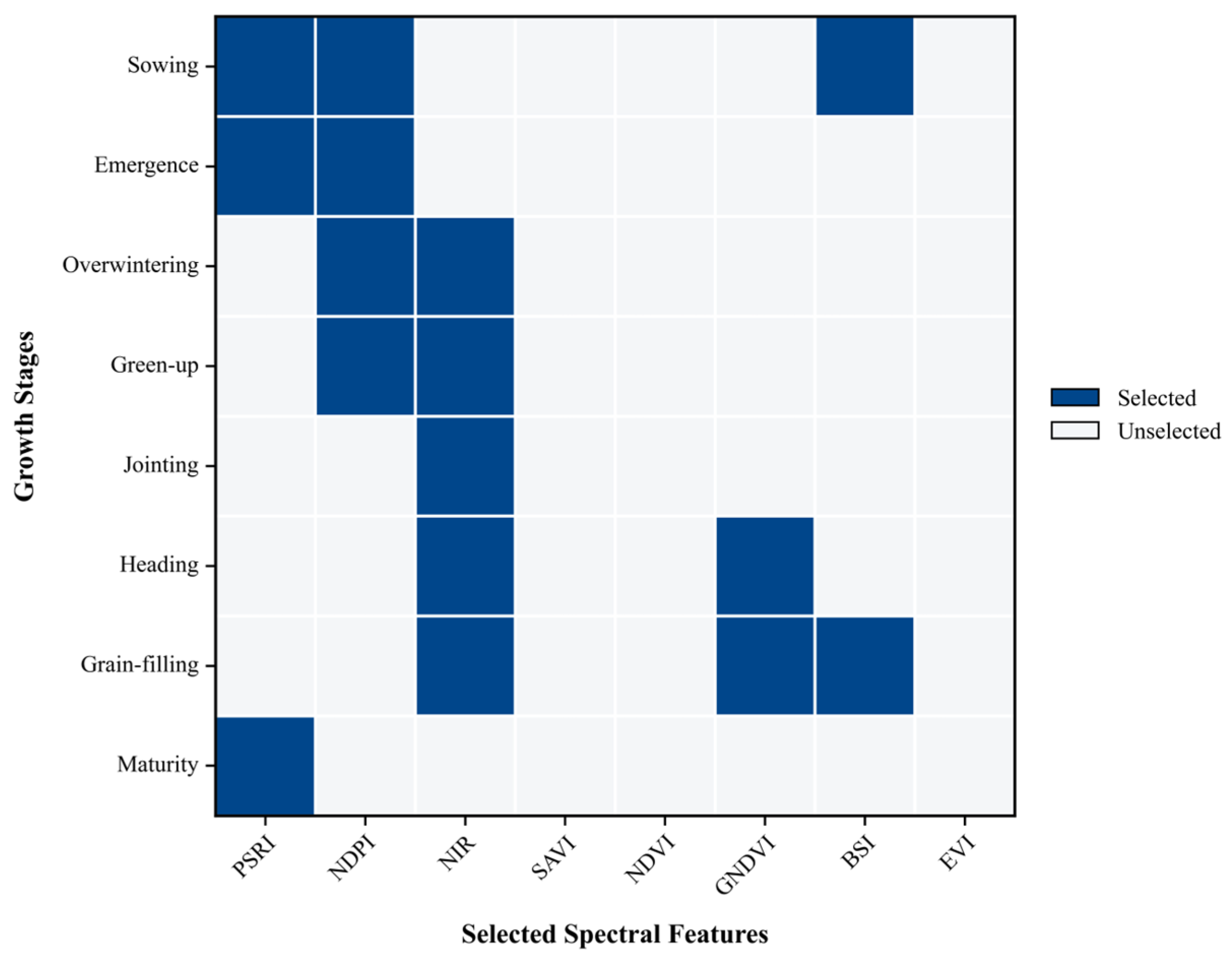
To analyze the behavior of key spectral variables across growth stages, the selected variables for each stage were summarized using a heatmap (Figure 12), where a value of 1 indicates that a variable was identified as a key feature.

The composition of key spectral variables varies across growth stages, while also showing partial overlap. At the sowing stage, PSRI, NDPI, and BSI were selected as key features, whereas at the emergence stage, NDPI and PSRI dominated. This indicates that under early low-vegetation conditions, spectral information related to senescence and soil background plays an important role in discrimination. During the overwintering and green-up stages, NDPI and near-infrared reflectance (NIR) were consistently selected, suggesting that NIR and vegetation indices are particularly effective at capturing weak vegetation signals.

Under the redundancy control strategy, the jointing and maturity stages exhibited strong feature concentration, with only one dominant variable retained—NIR and PSRI, respectively. This reflects the decisive role of stage-specific physiological characteristics in these periods. At the heading stage, GNDVI and NIR were identified as core features, while at the grain-filling stage, BSI, GNDVI, and NIR were jointly retained, indicating that multiple types of spectral information contribute complementarily during the transition from peak growth to senescence.

Further comparison reveals that several variables repeatedly appear across multiple growth stages, indicating consistent cross-stage representational capability. NDPI was consistently selected from the sowing to green-up stages, suggesting its usefulness for characterizing weak vegetation conditions. NIR appeared from the overwintering to grain-filling stages, reflecting its high sensitivity to canopy structure and growth dynamics. GNDVI was mainly associated with the heading and grain-filling stages, highlighting its effectiveness in capturing chlorophyll variation during vigorous growth. In contrast, PSRI was primarily selected in the sowing, emergence, and maturity stages, while BSI appeared mainly in the sowing and grain-filling stages, indicating their sensitivity to early sparse vegetation and late-stage senescence, respectively.

These results demonstrate that key spectral variables exhibit both stage specificity and cross-stage consistency. On the one hand, dominant features differ among growth stages, indicating that a single stage cannot fully represent the spectral characteristics of winter wheat throughout its growth cycle. On the other hand, certain variables repeatedly appear across stages, suggesting stable discriminative value.

These findings are consistent with previous studies. It has been shown that different growth stages correspond to different dominant features, while some core variables contribute continuously across multiple periods [35]. Omia et al. further emphasized that, for phenology-sensitive crops, selecting representative indices based on stage-specific physiological characteristics is more effective than simply stacking multiple spectral features [37].

Therefore, the results of key spectral variable selection not only reveal stage-dependent feature variation, but also highlight the importance of integrating stable cross-stage features. This provides an empirical basis for the progressive accumulation model (PAM) and the cross-temporal fusion model (CTFM), where both stage-specific and cross-stage information are jointly utilized.

4.4. Limitations and Future Work

Although the proposed framework achieved promising performance for winter wheat mapping in Shandong Province, several aspects could be further improved in future studies. First, this study was conducted using Sentinel-2 imagery from the 2023–2024 winter wheat growing season. Five-fold cross-validation was used to evaluate model stability under different sample partitions; however, multi-year validation would be useful for further assessing the influence of inter-annual variations in weather conditions, phenological development, and management practices. In addition, although the study area covers the main winter wheat-producing region of Shandong Province, further tests in other regions with different climatic conditions, cropping systems, and phenological calendars would help evaluate the broader applicability of the proposed framework.

Second, the sample dataset was obtained through manual visual interpretation and included both winter wheat and non-winter-wheat samples distributed across the study area. This sampling strategy supported model training and validation in the present study, but future work could further improve sample representativeness by incorporating field survey data, spatially stratified sampling, or independent validation samples. However, the random split may not fully guarantee spatial independence between training and validation samples, and residual spatial autocorrelation may still exist. Future studies should adopt block-based or prefecture-level spatial cross-validation to further assess spatial transferability. Similarly, the use of fixed growth-stage windows provided a consistent temporal framework for province-wide feature extraction, while dynamic phenological windows may better capture local differences in crop development.

Third, the CTFM used inter-stage mean and difference features to provide a compact and interpretable representation of multi-stage information. This design reduced feature dimensionality while maintaining high classification accuracy. Nevertheless, more detailed temporal descriptors, such as growth rate, peak timing, curve-fitting parameters, and harmonic features, could be explored in future studies to characterize complex phenological dynamics. Although a representative Temporal CNN baseline was included in this study, further comparisons with other advanced time-series models, such as LSTM, Transformers, and multi-source data fusion approaches, would help clarify the broader application scenarios of the proposed method. From an operational perspective, CTFM M6 requires observations from six growth stages and is therefore more suitable for middle-to-late season or post-season mapping; for near-real-time applications, intermediate models such as CTFM M3–M5 may provide a practical trade-off between timeliness and accuracy.

5. Conclusions

To improve regional-scale winter wheat mapping, this study developed a multi-stage identification framework integrating growth-stage ranking, key spectral variable selection, and cross-temporal feature fusion. The main conclusions are as follows:

(1)

The discriminative ability of winter wheat varied across growth stages. The jointing, overwintering, heading, and grain-filling stages showed relatively strong identification performance, whereas the sowing and maturity stages contributed less discriminative information.

(2)

By combining permutation importance with correlation constraints, the original 64-dimensional temporal–spectral feature space was reduced to 16 key variables. The selected variables, including NDPI, PSRI, NIR, GNDVI, and BSI, effectively represented the main spectral differences in winter wheat across growth stages.

(3)

Both PAM and CTFM improved winter wheat identification by integrating multi-stage information. PAM achieved the highest OA of 0.9689 at M7, while CTFM M6 achieved a comparable OA of 0.9658 using only 10 fused features. Considering both accuracy and feature dimensionality, CTFM M6 was selected as the optimal model.

(4)

Based on CTFM M6, a 10 m winter wheat distribution map of Shandong Province was generated. The estimated area showed good agreement with statistical yearbook data, with a municipal-scale R² of 0.947 and a provincial-scale relative error of 8.55%. These results indicate that the proposed feature selection and multi-stage fusion strategy can achieve reliable regional-scale mapping of winter wheat in Shandong Province during the 2023–2024 growing season.

References

1. Dong, J.; Pang, Z.; Fu, Y.; Peng, Q.; Li, X.; Yuan, W. Annual winter wheat mapping dataset in China from 2001 to 2020. Sci. Data 2024, 11, 1218. [Google Scholar] [CrossRef] [Scilit]
2. Dong, J.; Fu, Y.; Wang, J.; Tian, H.; Fu, S.; Niu, Z.; Han, W.; Zheng, Y.; Huang, J.; Yuan, W. Early-season mapping of winter wheat in China based on Landsat and Sentinel images. Earth Syst. Sci. Data 2020, 12, 3081–3095. [Google Scholar] [CrossRef] [Scilit]
3. Liu, J.K.; Zhong, S.Q.; Liang, W.H. Extraction of crop planting structure based on multi-temporal Landsat 8 OLI imagery. Remote Sens. Technol. Appl. 2015, 30, 775–783. (In Chinese) [Google Scholar]
4. Qi, L.; Liu, L.Y.; Zhao, C.J.; Wang, J.H.; Wang, J.D. Selection of Optimum Periods for Extracting Winter Wheat Based on Multi-temporal Remote Sensing Images. Remote Sens. Technol. Appl. 2008, 23, 154–160. (In Chinese) [Google Scholar]
5. Saini, R.; Ghosh, S.K. Crop classification on single-date Sentinel-2 imagery using random forest and support vector machine. Int. Arch. Photogramm. Remote Sens. Spat. Inf. Sci. 2018, XLII-5, 683–688. [Google Scholar] [CrossRef] [Scilit]
6. Vuolo, F.; Neuwirth, M.; Immitzer, M.; Atzberger, C.; Ng, W.-T. How much does multi-temporal Sentinel-2 data improve crop type classification? Int. J. Appl. Earth Obs. Geoinf. 2018, 72, 122–130. [Google Scholar] [CrossRef] [Scilit]
7. Inglada, J.; Arias, M.; Tardy, B.; Hagolle, O.; Valero, S.; Morin, D.; Dedieu, G.; Sepulcre, G.; Bontemps, S.; Defourny, P.; et al. Assessment of an operational system for crop type map production using high temporal and spatial resolution satellite optical imagery. Remote Sens. 2015, 7, 12356–12379. [Google Scholar] [CrossRef] [Scilit]
8. Zhang, R.Q.; Wang, S.A.; Gao, W.L.; Sun, W.J.; Wang, J.L.; Niu, L.A. Remote-sensing classification method of county-level agricultural crops using time-series NDVI. Trans. Chin. Soc. Agric. Mach. 2015, 46, 246–252. (In Chinese) [Google Scholar] [CrossRef]
9. Heupel, K.; Spengler, D.; Itzerott, S. A progressive crop-type classification using multitemporal remote sensing data and phenological information. PFG J. Photogramm. Remote Sens. Geoinf. Sci. 2018, 86, 53–69. [Google Scholar] [CrossRef] [Scilit]
10. Kussul, N.; Lavreniuk, M.; Kolotii, A.; Skakun, S.; Rakoid, O.; Shumilo, L. A workflow for sustainable development goals indicators assessment based on high-resolution satellite data. Int. J. Digit. Earth 2019, 13, 309–321. [Google Scholar] [CrossRef] [Scilit]
11. Belgiu, M.; Drăguţ, L. Random forest in remote sensing: A review of applications and future directions. ISPRS J. Photogramm. Remote Sens. 2016, 114, 24–31. [Google Scholar] [CrossRef] [Scilit]
12. Yang, S.; Gu, L.; Li, X.; Jiang, T.; Ren, R. Crop classification method based on optimal feature selection and hybrid CNN-RF networks for multi-temporal remote sensing imagery. Remote Sens. 2020, 12, 3119. [Google Scholar] [CrossRef] [Scilit]
13. Georganos, S.; Grippa, T.; Vanhuysse, S.; Lennert, M.; Shimoni, M.; Kalogirou, S.; Wolff, E. Less is more: Optimizing classification performance through feature selection in a very-high-resolution remote sensing object-based urban application. GISci. Remote Sens. 2018, 55, 221–242. [Google Scholar] [CrossRef] [Scilit]
14. Rouse, J.W., Jr.; Haas, R.H.; Schell, J.A.; Deering, D.W. Monitoring vegetation systems in the Great Plains with ERTS. In Proceedings of the Third Earth Resources Technology Satellite-1 Symposium; Freden, S.C., Mercanti, E.P., Becker, M.A., Eds.; NASA: Washington, DC, USA, 1974; pp. 309–317. [Google Scholar]
15. Huete, A.; Didan, K.; Miura, T.; Rodriguez, E.P.; Gao, X.; Ferreira, L.G. Overview of the radiometric and biophysical performance of the MODIS vegetation indices. Remote Sens. Environ. 2002, 83, 195–213. [Google Scholar] [CrossRef] [Scilit]
16. Huete, A.R. A soil-adjusted vegetation index (SAVI). Remote Sens. Environ. 1988, 25, 295–309. [Google Scholar] [CrossRef] [Scilit]
17. Miao, H.; Zhang, R.; Song, Z.; Chang, Q. Estimating winter wheat canopy chlorophyll content through the integration of unmanned aerial vehicle spectral and textural insights. Remote Sens. 2025, 17, 406. [Google Scholar] [CrossRef] [Scilit]
18. Xu, D.; Wang, C.; Chen, J.; Shen, M.; Shen, B.; Yan, R.; Li, Z.; Karnieli, A.; Chen, J.; Yan, Y.; et al. The superiority of the normalized difference phenology index (NDPI) for estimating grassland aboveground fresh biomass. Remote Sens. Environ. 2021, 264, 112578. [Google Scholar] [CrossRef] [Scilit]
19. Anderegg, J.; Yu, K.; Aasen, H.; Walter, A.; Liebisch, F.; Hund, A. Spectral vegetation indices to track senescence dynamics in diverse wheat germplasm. Front. Plant Sci. 2020, 10, 1749. [Google Scholar] [CrossRef] [Scilit]
20. Mzid, N.; Pignatti, S.; Huang, W.; Casa, R. An analysis of bare soil occurrence in arable croplands for remote sensing topsoil applications. Remote Sens. 2021, 13, 474. [Google Scholar] [CrossRef] [Scilit]
21. Brenes Fuentes, M.V.; Heenkenda, M.K.; Sahota, T.S.; Segura Serrano, L. Analyzing winter wheat (Triticum aestivum) growth pattern using high spatial resolution images: A case study at Lakehead University Agriculture Research Station, Thunder Bay, Canada. Crops 2024, 4, 115–133. [Google Scholar] [CrossRef] [Scilit]
22. Razaque, A.; Ben Haj Frej, M.; Almi’ani, M.; Alotaibi, M.; Alotaibi, B. Improved support vector machine enabled radial basis function and linear variants for remote sensing image classification. Sensors 2021, 21, 4431. [Google Scholar] [CrossRef] [Scilit]
23. Breiman, L. Random forests. Mach. Learn. 2001, 45, 5–32. [Google Scholar] [CrossRef] [Scilit]
24. Congalton, R.G.; Green, K. Assessing the Accuracy of Remotely Sensed Data: Principles and Practices, 3rd ed.; CRC Press: Boca Raton, FL, USA, 2019. [Google Scholar] [CrossRef] [Scilit]
25. Foody, G.M. Explaining the unsuitability of the kappa coefficient in the assessment and comparison of the accuracy of thematic maps obtained by image classification. Remote Sens. Environ. 2020, 239, 111630. [Google Scholar] [CrossRef] [Scilit]
26. Sokolova, M.; Lapalme, G. A systematic analysis of performance measures for classification tasks. Inf. Process. Manag. 2009, 45, 427–437. [Google Scholar] [CrossRef] [Scilit]
27. Maynard, J.J.; Levi, M.R. Hyper-temporal remote sensing for digital soil mapping: Characterizing soil-vegetation response to climatic variability. Geoderma 2017, 285, 94–109. [Google Scholar] [CrossRef] [Scilit]
28. Liu, S.; Peng, D.; Zhang, B.; Chen, Z.; Yu, L.; Chen, J.; Pan, Y.; Zheng, S.; Hu, J.; Lou, Z.; et al. The Accuracy of Winter Wheat Identification at Different Growth Stages Using Remote Sensing. Remote Sens. 2022, 14, 893. [Google Scholar] [CrossRef] [Scilit]
29. Liu, X.; Li, X.; Gao, L.; Zhang, J.; Qin, D.; Wang, K.; Li, Z. Early-season and refined mapping of winter wheat based on phenology algorithms: A case of Shandong, China. Front. Plant Sci. 2023, 14, 1016890. [Google Scholar] [CrossRef] [Scilit]
30. Dong, Q.; Chen, X.; Chen, J.; Zhang, C.; Liu, L.; Cao, X.; Zang, Y.; Zhu, X.; Cui, X. Mapping winter wheat in North China using Sentinel-2A/B data: A method based on phenology-time weighted dynamic time warping. Remote Sens. 2020, 12, 1274. [Google Scholar] [CrossRef] [Scilit]
31. Qiu, B.; Luo, Y.; Tang, Z.; Chen, C.; Lu, D.; Huang, H.; Chen, Y.; Chen, N.; Xu, W. Winter wheat mapping combining variations before and after estimated heading dates. ISPRS J. Photogramm. Remote Sens. 2017, 123, 35–46. [Google Scholar] [CrossRef] [Scilit]
32. Lv, S.; Xia, X.; Pan, Y. Optimization of characteristic phenological periods for winter wheat extraction using remote sensing in plateau valley agricultural areas in Hualong, China. Remote Sens. 2023, 15, 28. [Google Scholar] [CrossRef] [Scilit]
33. Yang, G.; Li, X.; Liu, P.; Yao, X.; Zhu, Y.; Cao, W.; Chen, T. Automated in-season mapping of winter wheat in China with training data generation and model transfer. ISPRS J. Photogramm. Remote Sens. 2023, 202, 422–438. [Google Scholar] [CrossRef] [Scilit]
34. Qu, C.; Li, P.; Zhang, C. A spectral index for winter wheat mapping using multi-temporal Landsat NDVI data of key growth stages. ISPRS J. Photogramm. Remote Sens. 2021, 175, 431–447. [Google Scholar] [CrossRef] [Scilit]
35. Liu, M.; He, W.; Zhang, H. WPS: A whole phenology-based spectral feature selection method for mapping winter crop from time-series images. ISPRS J. Photogramm. Remote Sens. 2024, 210, 141–159. [Google Scholar] [CrossRef] [Scilit]
36. Weiss, M.; Jacob, F.; Duveiller, G. Remote sensing for agricultural applications: A meta-review. Remote Sens. Environ. 2020, 236, 111402. [Google Scholar] [CrossRef] [Scilit]
37. Omia, E.; Bae, H.; Park, E.; Kim, M.S.; Baek, I.; Kabenge, I.; Cho, B.-K. Remote sensing in field crop monitoring: A comprehensive review of sensor systems, data analyses and recent advances. Remote Sens. 2023, 15, 354. [Google Scholar] [CrossRef] [Scilit]
Figure 1. Location of the study area
Remotesensing 18 01927 g001
Figure 2. Spatial distribution of winter wheat and non-wheat sample points.
Remotesensing 18 01927 g002
Figure 3. Technical framework. The yellow star indicates the optimal model selected based on the accuracy–complexity trade-off analysis.
Remotesensing 18 01927 g003
Figure 4. Temporal variation curves of spectral variables for wheat and non-wheat samples across different growth stages. The shaded area is used to highlight the difference between wheat and non-wheat samples across growth stages.
Remotesensing 18 01927 g004
Figure 5. Accuracy comparison of single-growth-stage models: (a) overall accuracy (OA); (b) Kappa coefficient; (c) F1-score; (d) user’s accuracy (UA); and (e) producer’s accuracy (PA).
Remotesensing 18 01927 g005
Figure 6. Five-fold cross-validation OA ranking of single-stage RF models. Error bars indicate standard deviations.
Remotesensing 18 01927 g006
Figure 7. Correlation distribution characteristics of spectral variables across growth stages (Pearson correlation coefficient). Each subplot (a–h) corresponds to one growth stage: (a) Sowing, (b) Emergence, (c) Overwintering, (d) Green-up, (e) Jointing, (f) Heading, (g) Grain-filling, and (h) Maturity.
Remotesensing 18 01927 g007
Figure 8. Distribution of permutation importance across growth stages.
Remotesensing 18 01927 g008
Figure 9. Classification performance and feature dimensionality changes in the progressive accumulation model and the cross-temporal fusion model across growth stages.
Remotesensing 18 01927 g009
Figure 10. Spatial distribution of winter wheat in Shandong Province during the 2023–2024 growing season.
Remotesensing 18 01927 g010
Figure 11. Comparison and validation of remotely sensed winter wheat area and statistical yearbook data in Shandong Province.
Remotesensing 18 01927 g011
Figure 12. Distribution of key spectral variable selection across growth stages.
Remotesensing 18 01927 g012