A Multi-Level Cross-Modal Edge Filtering Method for High-Resolution Optical-SAR Image Registration

Highlights

What are the main findings?

• We construct a large-scale, high-resolution optical–SAR registration dataset, pairing 3-m SAR imagery from the HongTu-1 satellite with Google Earth optical imagery at zoom level 17, covering the major geographical regions of China, and we release the standardized pipeline—including full-scene pairing, DEM-based terrain correction, geometric refinement, standardized 512 × 512 slicing and multi-stage quality filtering—that was used to build it.
• Our proposed Log-domain reformulation of the Total Variation (Log-TV) filter substantially improves SAR image preprocessing by converting the multiplicative speckle noise model into an additive one, thereby enabling effective suppression of speckle while preserving edge structures and providing a much cleaner foundation for subsequent keypoint detection.
• Combining a machine learning-based edge filter (Structured Random Forest, SRF) with the hand-crafted phase congruency filter yields a strong synergistic effect for cross-modal optical–SAR edge filtering, producing more stable and consistent shared structural responses than either component alone.

What are the implications of the main findings?

• Large-scale, high-resolution optical–SAR datasets are both essential and scarce for registration and other downstream tasks. Only on larger and more complex benchmarks do the robustness and the true relative performance of competing algorithms become evident, making such datasets a necessary foundation for future research in this area.
• Different imaging modalities require different filtering strategies: for heavily speckled data such as SAR imagery, regularisation in the logarithmic domain is more appropriate than directly applying denoisers designed for additive noise, highlighting the importance of modality-aware preprocessing in cross-modal registration.
• Hybrid pipelines that integrate learning-based components with hand-crafted filters are a promising direction: beyond edge filtering, similar combinations of deep features and classical hand-crafted operators may also benefit cross-modal feature description and matching stages.

Abstract

Optical and Synthetic Aperture Radar (SAR) image registration is a fundamental task in remote sensing information fusion, yet it remains challenging due to significant differences in imaging mechanisms, radiation characteristics, and noise properties between the two modalities. Existing public datasets suffer from limited resolution, small scale, and insufficient scene diversity, and these limitations have hindered algorithm development. This paper constructs a large-scale, high-resolution optical–SAR registration dataset based on the HongTu-1 satellite 3-m SAR imagery and Google Earth optical imagery at zoom level 17, covering diverse scenes across China with a standardized pipeline including terrain correction, geometric alignment, standardized slicing, and quality filtering. Building upon this dataset, a hand-crafted keypoint-based cross-modal registration method is proposed, incorporating multi-level edge filtering and hybrid feature detection. Unlike conventional hand-crafted methods such as RIFT, SRIF, and LNIFT, which mainly refine keypoint detection, description, or matching within a SIFT-style pipeline, the core novelty of this work lies in SAR-specific preprocessing and multi-level hybrid filtering. These components are designed to suppress speckle while extracting more stable and discriminative shared edge responses for cross-modal registration. An improved Log-domain Total Variation (Log-TV) denoising model is introduced for SAR preprocessing. A hybrid edge filtering framework combining phase congruency analysis and Structured Random Forest (SRF) edge detection is constructed within a Gaussian scale space. A dual-branch feature detection scheme integrating blob and corner features is designed with a robust orientation assignment strategy. Feature description uses the Gradient Location–Orientation Histogram (GLOH) descriptor with Principal Component Analysis (PCA) reduction, while geometric estimation employs the Fast Sample Consensus (FSC) algorithm. Experiments on the self-constructed HT dataset and on the public OSdataset and SAR2Opt benchmarks show that the proposed method consistently achieves low RMSE and high success rates. It also maintains competitive efficiency among hand-crafted methods while retaining strong robustness to scale and rotation variations.

1. Introduction

For downstream remote-sensing tasks such as object detection [1,2,3,4,5,6], instance segmentation [7,8,9,10], image fusion [11,12] and change detection [13,14,15,16,17], cross-modal registration is a critical preprocessing step. Reliable spatial alignment is required before the complementary information carried by optical and SAR imagery can be fused under a common geographic reference. Once noticeable registration errors are introduced, the consistency of object locations, structural boundaries, and semantic regions across modalities is inevitably degraded, which in turn compromises the reliability of subsequent multi-temporal analysis, cross-modal knowledge transfer, and quantitative evaluation. Therefore, accurate and robust cross-modal registration should be regarded not only as an independent research problem but also as an essential foundation for higher-level remote-sensing interpretation tasks.

Hand-crafted optical and SAR image registration methods form a well-established class of algorithms that follow the conventional keypoint-based registration paradigm. These methods sequentially perform keypoint extraction, dominant orientation assignment, feature descriptor construction, feature matching, and geometric transformation model estimation. Their main improvements are typically concentrated in the front-end feature construction stage, particularly in multi-level filters, structural enhancement strategies, and feature response extraction mechanisms designed to address cross-modal differences. By enhancing image textures, edges, or local structural information in a targeted manner, these algorithms can alleviate the radiometric differences and noise interference between optical and SAR images to some extent, thereby improving the stability of subsequent feature extraction and matching.

In comparison, these methods generally still adopt basic strategies similar to SIFT [18] for feature description, matching filtering, and geometric transformation estimation. Their innovations are more reflected in the preprocessing, filtering, and feature detection stages rather than in restructuring the entire registration pipeline. Since they do not rely on large-scale training data, these hand-crafted algorithms possess strong interpretability and good cross-scene generalization capabilities. Meanwhile, the relationships between their processing modules are clear, facilitating analysis of how different steps affect the final registration performance. Therefore, improving preprocessing methods, filter structure design, and feature orientation assignment strategies for cross-modal images remains an important research direction in hand-crafted optical–SAR image registration.

Due to Nonlinear Radiation Distortions (NRDs), cross-modal images exhibit significant differences in grayscale response and local texture representation [19,20,21,22,23,24]. For optical-SAR image registration tasks, the multiplicative speckle noise prevalent in SAR images is one of the important factors affecting registration performance [25,26,27]. This type of noise not only weakens the discriminability of local structures but also interferes with keypoint detection, dominant orientation assignment, and descriptor construction, thereby reducing matching stability and registration accuracy.

In the field of edge detection, Dollár et al. [28] proposed the Structured Random Forest (SRF) method, which models edge detection as a structured prediction problem of local image patches. However, SRF is primarily designed for natural optical images and tends to produce weak edge responses when directly applied to SAR images due to speckle noise and nonlinear radiometric differences. Phase congruency-based structural features [29] have been widely used for robust cross-modal matching, as they maintain stable responses under intensity scaling, contrast changes, and even certain degrees of modal differences.

Existing hand-crafted registration algorithms such as OS-SIFT [30], RIFT [31], MS-HLMO [32], LNIFT [33], and 3MRS [34] have made notable contributions, but they still face limitations in handling high-resolution SAR with strong speckle noise and significant cross-modal discrepancies while registering with optical images.

Compared with RIFT, SRIF, and LNIFT, whose main improvements are concentrated in keypoint detection, descriptor construction, or matching refinement within a conventional SIFT-style pipeline, the principal innovation of this study lies in the SAR-oriented front end. By combining Log-TV preprocessing with a multi-level hybrid edge filtering design, the proposed method suppresses speckle and modality-induced radiometric inconsistency before keypoint extraction, thereby producing more robust and accurate structural responses for subsequent registration.

This paper proposes a cross-modal registration method based on the hand-crafted keypoint paradigm, accompanied by a self-constructed large-scale high-resolution dataset, with the following key contributions:

• A large-scale, high-resolution optical–SAR registration dataset is constructed based on HongTu-1 satellite 3-m SAR imagery and Google Earth [35] optical imagery at zoom level 17, covering diverse scenes across China with a standardized pipeline including terrain correction, geometric alignment, standardized slicing, and multi-stage quality filtering;
• An improved Log-domain Total Variation (Log-TV) denoising model for SAR image preprocessing that effectively suppresses multiplicative speckle noise while preserving edge structures;
• A hybrid edge filtering framework that combines phase congruency analysis with SRF edge detection within a multi-scale Gaussian scale space, enabling stable extraction of cross-modal shared structural information;
• A dual-branch feature detection scheme combining blob and corner features, with a robust orientation assignment strategy that integrates histogram-based and centroid-based methods.

2. Related Work

Optical and SAR images differ fundamentally in their imaging mechanisms, leading to large discrepancies in intensity distribution, texture appearance, speckle characteristics, and local geometric deformation [36,37,38]. Single-modality registration techniques therefore cannot be applied directly to optical–SAR scenarios, and a substantial body of work has extended the classical SIFT-style pipeline—feature detection, description, matching, and parametric transformation estimation—along three complementary directions: (i) cross-modal filtering and structural enhancement to reduce the gap between modalities [39]; (ii) modality-aware feature detection and descriptor design for more consistent representations [40]; and (iii) robust outlier rejection and model estimation to mitigate mismatches [41].

Cross-modal filtering and feature design. Because optical and SAR sensors obey distinct physical models, nonlinear radiometric distortions are unavoidable; recent work therefore designs filters that suppress modality-specific noise while emphasising shared structures. RIFT adopts phase congruency for keypoint detection and a maximum-index-map descriptor that replaces gradient histograms, providing strong robustness across optical, infrared, SAR and depth imagery. LNIFT reduces inter-modal radiometric differences through locally normalised filtering and operates in the spatial domain. On the detection side, OS-SIFT uses multi-scale Sobel operators on optical images and the ROEWA operator on SAR so that the two modalities yield more comparable gradient maps; subsequent works further enrich the gradient computation and inject scale/orientation information into matching. On the descriptor side, MS-HLMO introduces a multi-scale histogram of local main orientations to handle intensity, rotation and scale variations. CFOG-style channel-of-oriented-gradients descriptors are faster and more accurate than [42] for multi-modal template matching. WSSF [43] constructs weighted structural saliency features by integrating pointwise shape-adaptive texture filtering, steerable filtering and phase-based representations, enabling more reliable matching under severe nonlinear radiometric distortions. Compared with gradient-dominated descriptors, the method relies more heavily on structural consistency and therefore exhibits improved robustness in low-texture and cross-modal scenarios.

Matching, outlier rejection, and limitations. The matching stage commonly relies on fixed-threshold matching, nearest-neighbour matching, or the nearest-neighbour distance-ratio test, all of which still leave outliers. RANSAC [44] repeatedly samples minimal subsets, fits a candidate model, partitions correspondences into inliers and outliers, and retains the model with the largest inlier set; FSC [45] introduces a high-confidence subset together with a large consensus set and refines the model through an iterative consensus mechanism, obtaining more correct correspondences in fewer iterations. More recently, learning-based matchers have pushed correspondence quality substantially further on natural-image benchmarks: SuperGlue [46] formulates matching as an attention-based graph-neural-network problem over sparse keypoints, jointly reasoning about appearance and geometric context to reject outliers; LoFTR [47] removes the detector stage altogether and produces dense coarse-to-fine correspondences with a transformer, which is particularly effective in low-texture regions where classical keypoint detectors fail; and LightGlue [48] revisits the SuperGlue architecture with adaptive iteration depth, achieving comparable accuracy at a fraction of the inference cost and making learned matching practical for large-scale registration. Despite this maturity, hand-crafted optical–SAR registration remains limited in three ways: it relies heavily on hand-crafted features that only partially close the radiometric gap on dense urban scenes and under heavy speckle; it underuses higher-level semantic and contextual cues, hurting performance in low-texture or repetitive regions; and its performance is closely tied to the resolution and scene diversity of the evaluation data—no existing method consistently outperforms the others as resolution and inter-region differences increase. These observations motivate the dataset and the multi-level edge-filtering pipeline introduced below.

3. High-Resolution Optical–SAR Registration Dataset

3.1. Motivation and Overview

Although optical–SAR image registration technology has important application value in remote sensing information fusion, target detection, change monitoring, and scene understanding, its further development is still significantly constrained by the scarcity of high-quality public datasets. Currently available public optical–SAR registration datasets are relatively limited in number and generally suffer from small data scales, low image resolution, single scene types, insufficient control point accuracy, and inconsistent annotation quality. In particular, standardized high-resolution data for complex urban scenes, diverse land-cover distributions, and multi-temporal imaging conditions remain scarce, greatly limiting the training effectiveness, robustness verification, and fair comparison of existing registration algorithms, especially data-driven deep learning methods.

Representative public datasets include OSdataset [49] based on GaoFen-3 imagery, and SEN12MS [50]. OSdataset has promoted the open data sharing of optical–SAR registration research to some extent, but its optical data uses single-channel format, limiting the full utilization of texture and spectral information. SEN12MS has larger data scale and wider spatial coverage, but its 10 m spatial resolution and 256 × 256 slice size are mainly oriented toward multi-modal remote sensing scene classification, with limitations in image detail expression and high-resolution registration task adaptability. Additionally, QXS-SAROPT [51] provides SAR data from GaoFen-3 and optical data from Google Earth for registration tasks. SAR2Opt [52] pairs 1-m TerraSAR-X SAR images with co-registered Google Earth Engine optical tiles of $600\times 600$ pixels and contains roughly six thousand pairs; although it was originally curated for GAN-based SAR-to-optical translation rather than registration, its high spatial resolution and geographically diverse urban scenes make it a useful complementary benchmark for cross-modal matching, where the limited dataset size (a few thousand pairs) remains the main bottleneck for training and large-scale evaluation. A summary comparison of representative datasets is provided in

Table 1. Comparison of the self-constructed dataset with other large-scale paired datasets.

Dataset	SAR Source	Resolution	Slice Size	Pairs
OSdataset	GaoFen-3	1-m (SAR)	256 × 256 & 512 × 512	10,692
SEN12MS	Sentinel-1	10-m	256 × 256	180,662
QXS-SAROPT	GaoFen-3	1-m (SAR)	256 × 256	20,000
Ours (HT)	HongTu-1	3-m (SAR)/1-m (Opt.)	512 × 512	30,733

.

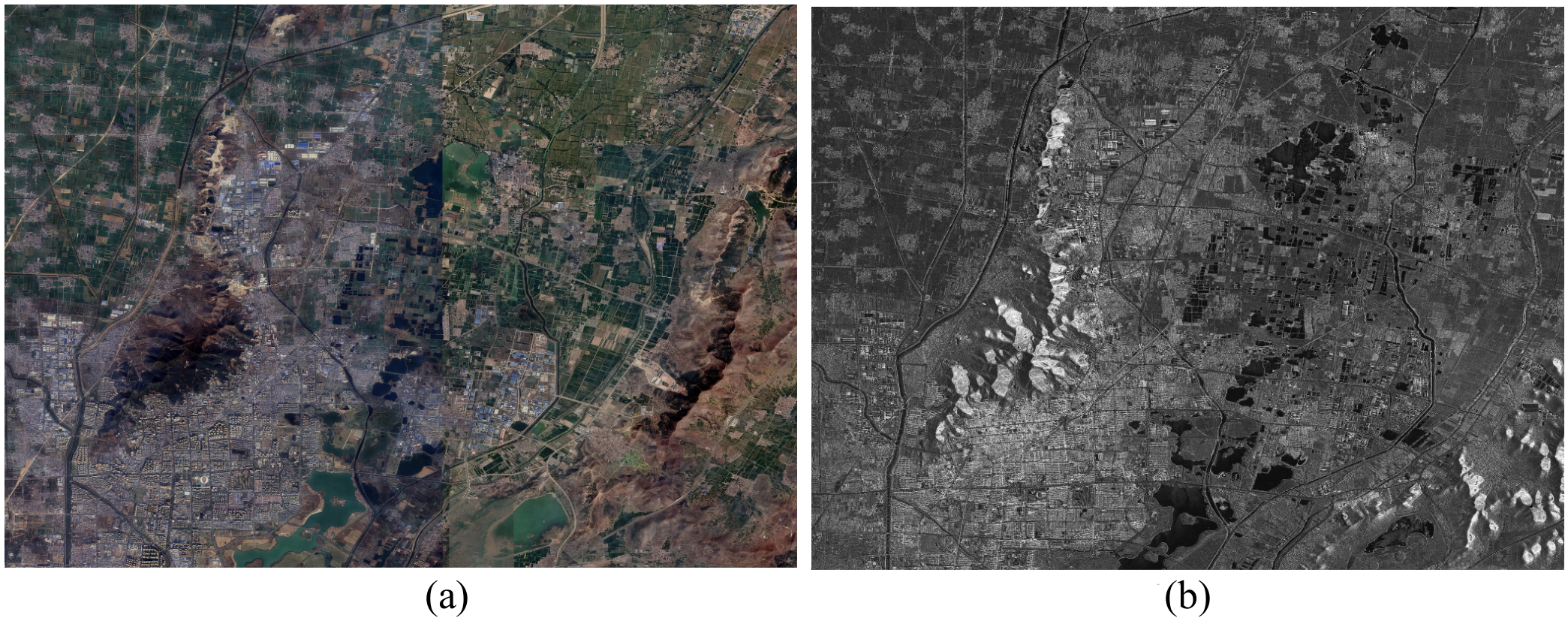
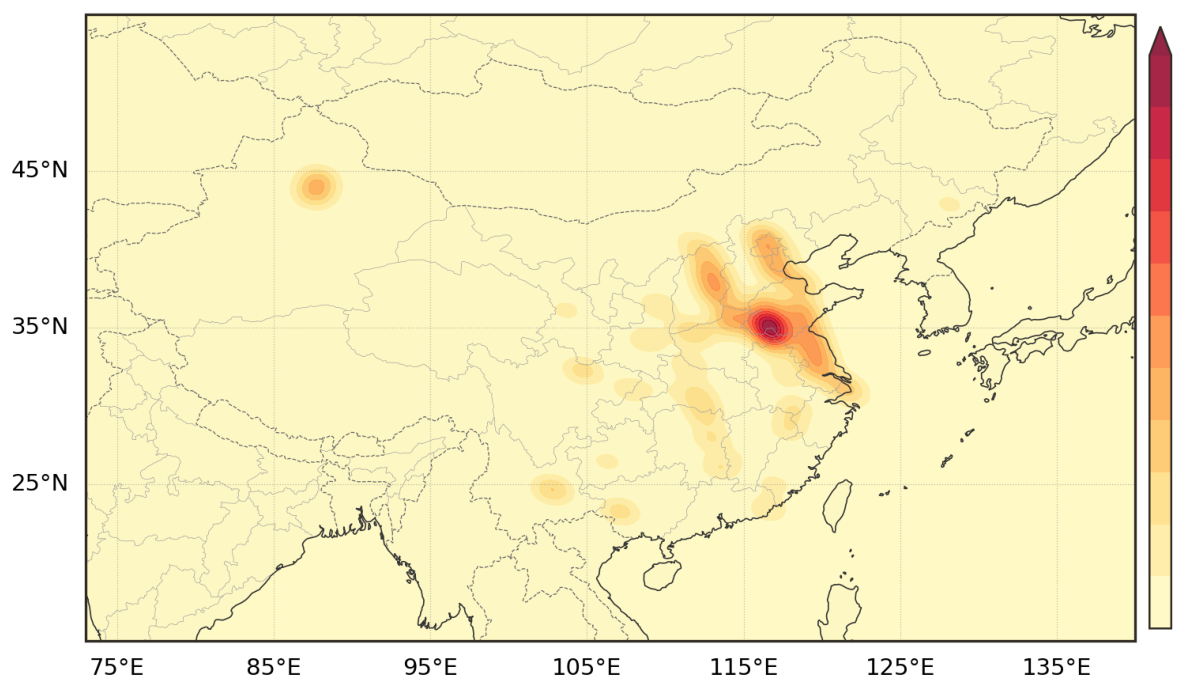
To address these limitations, this paper constructs a dedicated dataset for optical–SAR image registration tasks. The dataset uses SAR images acquired by the domestic HongTu-1 series satellite (PIESAT Information Technology Co., Ltd., Beijing, China) at 3-m resolution, paired with corresponding Google Earth optical imagery at zoom level 17 (approximately 1-m resolution). Figure 1 presents an example of a full-scene optical and SAR image pair, in which the optical image exhibits visible stitching seams caused by multi-temporal compositing, while the SAR image displays typical speckle noise characteristics. The spatial coverage of the dataset spans the major geographical regions of China, with collection sites distributed across the Northeast, North, Northwest, Central, East, Southwest, and South regions to ensure scene diversity, as illustrated by the sampling distribution heatmap in Figure 2. The dataset construction process fully considers the requirements of registration tasks for geometric consistency, scene diversity, and annotation reliability.

3.2. Dataset Construction Pipeline

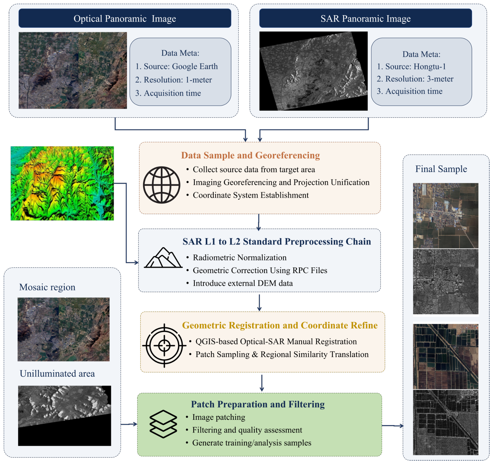
The dataset construction follows a standardized pipeline as illustrated in Figure 3, comprising the following steps:

(1) Data Sample and georeferencing. Optical remote sensing images and SAR images within the study area are selected as basic data pairs. Using the spatial extent of one SAR scene as the reference, the corresponding sub-image from the optical image is extracted through boundary-box-based cropping, ensuring spatial coverage consistency between the optical and SAR images.

(2) SAR L1 to L2 Standard Preprocessing Chain. Starting from L1 SAR products, we first perform radiometric normalization/calibration using scene metadata (META information) to ensure consistent backscatter representation across acquisition conditions. We then apply geometric correction based on the Rational Polynomial Coefficient (RPC) file to improve geolocation consistency at the sensor-model level. A Digital Elevation Model (DEM) is introduced for terrain correction of SAR images [53,54]. The SRTM (Shuttle Radar Topography Mission) [55] elevation data is used, which covers most global land areas with public accessibility and good compatibility with mainstream SAR processing chains. Due to the side-looking imaging nature of SAR, terrain undulations cause geometric distortions such as layover, shadow, and foreshortening. Radiometric Terrain Correction (RTC) is further applied to normalize the SAR imagery to a more stable scattering representation, reducing the influence of terrain on brightness and scattering intensity [56].

(3) Geometric registration and coordinate refinement. We first perform a preliminary manual registration using the QGIS toolbox (QGIS 3.34) [57] to obtain an initial coarse alignment between optical and SAR images. Then the terrain-corrected SAR image is processed through block slicing. Randomly sampled paired slices are matched using regional similarity algorithms at different displacement parameters, maximizing window similarity after translation. The average translation across all sampled slices yields translation parameters converted to a coordinate transformation matrix. This matrix is applied to the optical image through coordinate transformation algorithms (affine or projective), mapping optical pixel coordinates to the SAR geometric reference frame.

(4) Patch preparation and filtering. Since full-scene optical and SAR images are too large for mainstream deep learning model inputs, matching image pairs are cut into 512 × 512 pixel slices using overlapping windows with uniform sampling, following the standard adopted by OSdataset, balancing data volume and computational efficiency. Due to the limited observation range of SAR radar, pixels outside the observation range are set to zero, creating black edges. A high-frequency energy metric is computed using Sobel operators to measure texture richness:

$${\mathit{G}}_x={\mathit{S}}_x\ast \mathit{I},{\mathit{G}}_y={\mathit{S}}_y\ast \mathit{I}$$

(1)

where ∗ denotes 2D convolution, $\mathit{I}$ is the input image, and ${\mathit{S}}_x$, ${\mathit{S}}_y$ are the horizontal and vertical Sobel kernels.

The edge energy is computed as the mean squared gradient magnitude:

$$E={\displaystyle \frac{1}{N}}\sum _i({\mathit{G}}_x^2\left(i\right)+{\mathit{G}}_y^2\left(i\right))$$

(2)

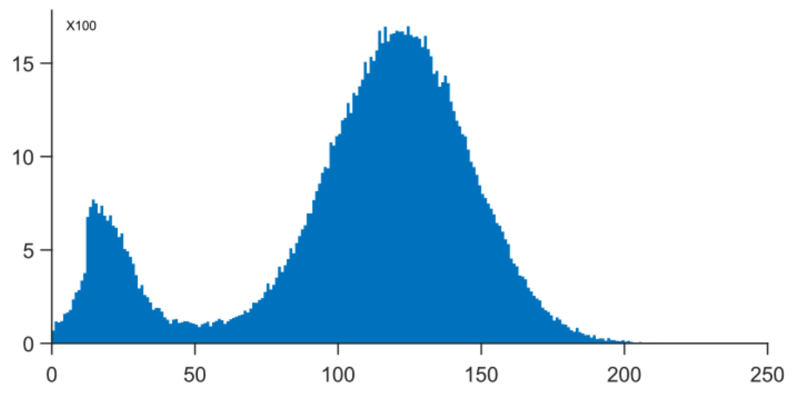
The energy distribution exhibits a clear bimodal pattern, as shown in Figure 4, enabling threshold-based separation of texture-rich regions from featureless areas. In practice, the threshold is set to 70, which is selected from the valley between the two peaks in the distribution to filter out texture-deficient slices and prevent low-texture regions from entering the final dataset. Slices with rich textures and strong cross-modal complementarity (urban areas, farmland, etc.) are retained, while uniform regions (black borders, textureless areas) are filtered out.

Additionally, optical images contain stitching seams from Google Earth multi-temporal compositing. A Vision–Language Model (Qwen3-VL-8B-Instruct [58]) is employed for binary classification to detect and filter out slices containing stitching artifacts.

3.3. Dataset Description

The dataset covers SAR data collected nationwide across China, including the Northeast, North China, East China, South China, Central China, Northwest, and Southwest regions, with a small amount of international data. The dataset primarily targets texture-complex urban scenes, also including ports, mountainous areas, desert terrain, and plains/farmland. The original SAR data has a physical resolution of approximately 3-m, and the optical data resolution is approximately 1-m.

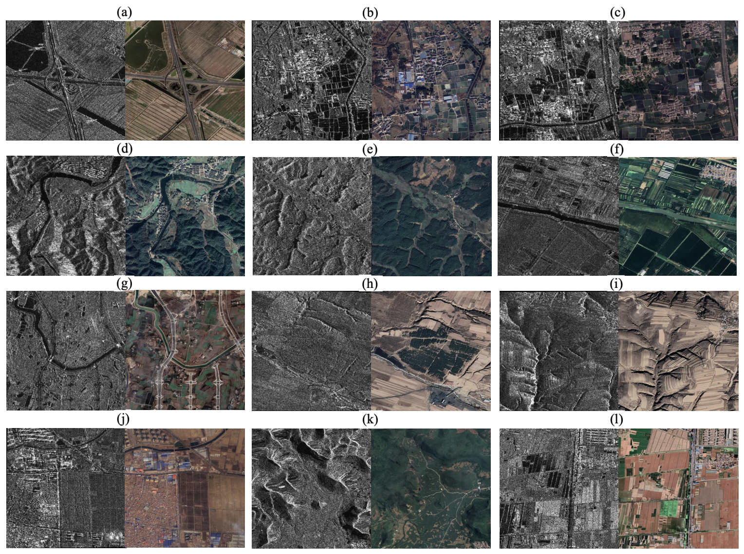
Figure 5 shows a random preview of 512 × 512 paired slices drawn from the final dataset, with each column presenting an optical tile alongside its co-registered SAR counterpart and covering a mix of urban, port, mountainous, desert and farmland scenes. After the complete construction pipeline, the two modalities are visually well aligned on shared structures such as road networks, coastlines and building blocks while still retaining the distinct radiometric and textural signatures of each modality (e.g., speckle and bright scatterers in SAR, spectral colour and fine texture in optical), providing a representative and diverse set of samples for cross-modal registration evaluation.

3.4. Geometric Transformation Models

For subsequent algorithm verification and validation set construction, the geometric transformation models used in this paper are introduced. Image registration aims to find a spatial transformation function that aligns the overlapping region between two images. Throughout the mathematical derivations, scalar variables are set in italic, vectors and matrices are set in bold italic, and named operators or functions are set in upright font.

The affine transformation, suitable for locally planar scenes with small viewpoint changes, describes translation, rotation, scaling, and shearing in 2D. For a 2D point $\mathit{x}$ with homogeneous coordinate $\tilde{\mathit{x}}$, the affine transformation is:

$${\tilde{\mathit{x}}}^{\prime }=\left[\begin{array}{cc}\mathit{A}& \mathit{t}\\ {\mathbf{0}}^{\top }& 1\end{array}\right]\tilde{\mathit{x}}$$

(3)

where $\mathit{A}\in {\mathbb{R}}^{2\times 2}$ represents the linear transformation and $\mathit{t}\in {\mathbb{R}}^2$ is the translation. The affine model has 6 degrees of freedom, requiring at least 3 non-degenerate point pairs for solution.

The projective transformation (homography) for more significant viewpoint differences is expressed as:

$$\lambda {\tilde{\mathit{x}}}^{\prime }=\mathit{H}\tilde{\mathit{x}}=\left[\begin{array}{ccc}{h}_{11}& h_{12}& h_{13}\\ h_{21}& h_{22}& h_{23}\\ h_{31}& h_{32}& h_{33}\end{array}\right]\tilde{\mathit{x}}$$

(4)

where $\lambda$ is the scale factor. Since homography is equivalent up to scale, it has 8 effective degrees of freedom, requiring at least 4 non-collinear point pairs. In practice, both models are combined with RANSAC-type robust estimation.

3.5. Dataset Validation

A subset of data was extracted to construct a validation set for subsequent registration algorithm performance verification. The reference evaluation metric used here is the Root Mean Square Error (RMSE). For each test image pair, K control point pairs are selected, where ${\mathit{p}}_k$ is located in the reference image and ${\mathit{p}}_k^{\prime }$ is its correspondence. Given the estimated transformation $\widehat{\mathit{H}}$, the point-wise geometric error for the k-th pair is defined as:

$$e_k={\parallel \widehat{\mathit{H}}{\mathit{p}}_k-{\mathit{p}}_k^{\prime }\parallel }_2$$

(5)

$$\mathrm{RMSE}=\sqrt{{\displaystyle \frac{1}{K}}\sum _{k=1}^K{e}_k^2}$$

(6)

Without applying random geometric transformations, a subset of urban terrain with clear textures was extracted, and several representative hand-crafted optical–SAR registration algorithms (HPOC [59] and CFOG [60]) were evaluated on this subset to verify the geometric quality of the dataset. The results are reported in

Table 2. Performance of representative hand-crafted optical–SAR registration algorithms on the dataset validation subset (no random geometric transformation applied).

Method	HPOC	CFOG	Manually Annotated Control Point
Avg. RMSE	2.71	2.53	1.33
Time (s)	142.35	7.89	N/A

. Both methods achieve low RMSE values, indicating good global geometric consistency of the data pairs. In particular, the manually annotated control points achieving lower RMSE values further confirm that this validation subset provides reliable geometric alignment quality.

4. Materials and Methods

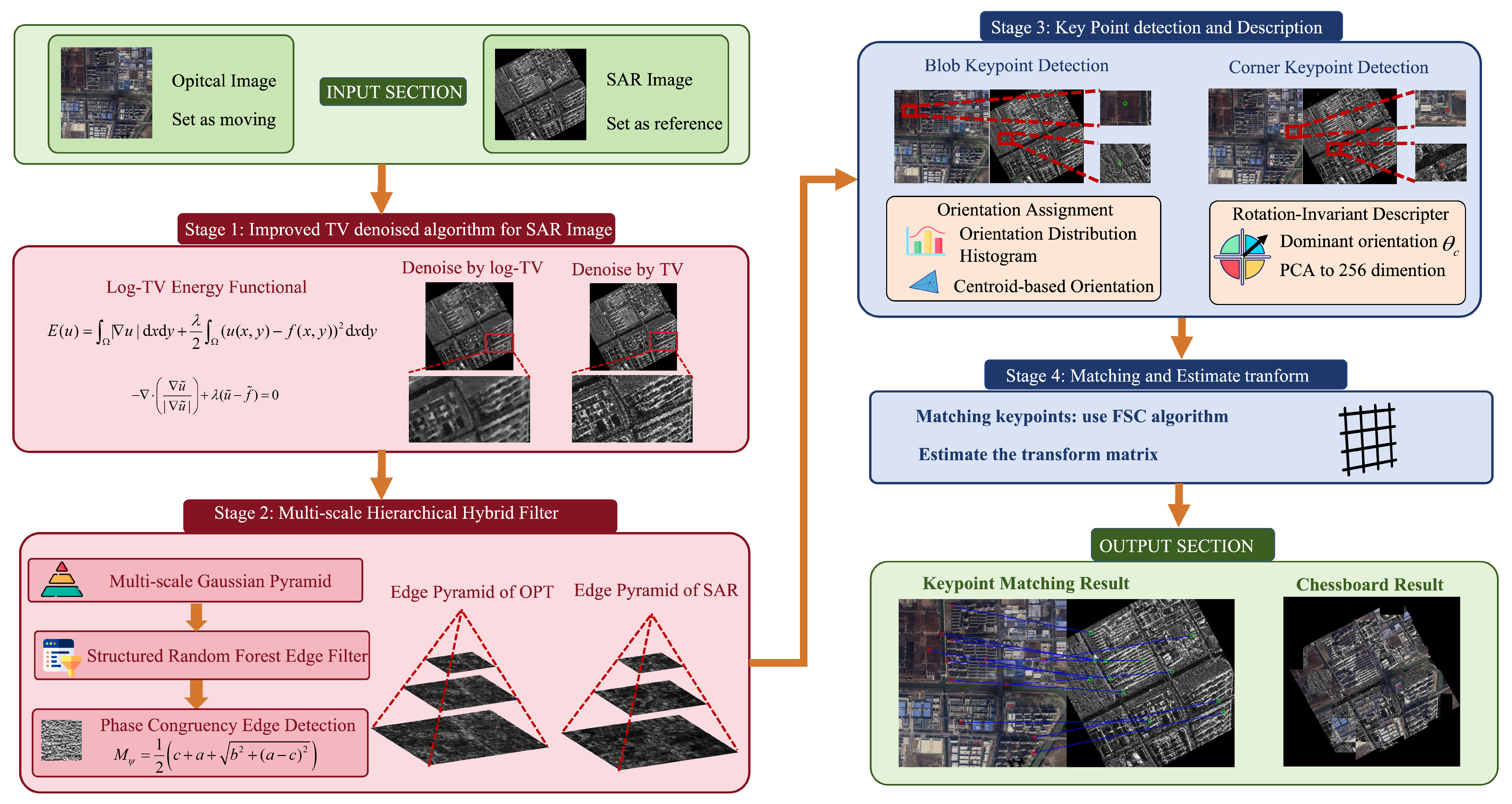
An overview of the proposed registration pipeline is given in Figure 6; the remainder of this section details each stage.

4.1. SAR Image Preprocessing

Before feature extraction, SAR images need to be preprocessed in order to reduce the radiometric inconsistency between modalities and enhance stable structural information. This paper builds on the Total Variation (TV) denoising model of Rudin et al. [61]: by imposing an $L_1$-type constraint on the image gradient, TV suppresses high-frequency oscillatory noise while preserving the discontinuities that correspond to image edges, which is in general a more edge-friendly choice than linear smoothing or $L_2$-based regularisers.

Under the additive Gaussian noise assumption $\mathit{f}=\mathit{u}+\mathit{\eta }$, where $\mathit{f}$ is the observed image on a bounded domain $\Omega$ and $\mathit{u}$ is the underlying clean image, the TV estimate is obtained by minimising

$$E\left(\mathit{u}\right)={\int }_{\Omega }|\nabla \mathit{u}|\mathrm{d}x+{\displaystyle \frac{\lambda }{2}}{\int }_{\Omega }{(\mathit{f}-\mathit{u})}^2\mathrm{d}x,$$

(7)

in which the first term suppresses noise oscillations while permitting finite jumps at object boundaries, the second term enforces fidelity to the observation, and $\lambda$ balances the two.

However, the standard TV denoising model is not ideal for SAR image denoising because SAR images are affected by multiplicative speckle noise, while the TV model assumes additive Gaussian noise. For multiplicative noise, the common approach is to apply a logarithmic transform to convert it into an additive noise problem. The SAR image noise model is:

$$\mathit{f}=\mathit{u}\odot \mathit{\eta }$$

(8)

where $\mathit{f}$ is the observed noisy image, $\mathit{u}$ is the desired noise-free image, and $\mathit{\eta }$ is the multiplicative noise term (typically assumed to follow a Gamma or Rayleigh distribution). Taking the logarithm of both sides:

$$ln\mathit{f}=ln\mathit{u}+ln\mathit{\eta }$$

(9)

In many practical cases, $ln\mathit{\eta }$ can be approximately treated as additive noise with constant mean. Denoting $\tilde{\mathit{f}}=ln\mathit{f}$, $\tilde{\mathit{u}}=ln\mathit{u}$, and $\tilde{\mathit{\eta }}=ln\mathit{\eta }$, we obtain the standard additive noise model $\tilde{\mathit{f}}=\tilde{\mathit{u}}+\tilde{\mathit{\eta }}$. The Log-TV energy functional can then be constructed as:

$$E\left(\tilde{\mathit{u}}\right)={\int }_{\Omega }|\nabla \tilde{\mathit{u}}|\mathrm{d}x+{\displaystyle \frac{\lambda }{2}}{\int }_{\Omega }{(\tilde{\mathit{f}}-\tilde{\mathit{u}})}^2\mathrm{d}x$$

(10)

The Euler–Lagrange equation of the Log-TV model is:

$$-div\left({\displaystyle \frac{\nabla \tilde{\mathit{u}}}{|\nabla \tilde{\mathit{u}}|}}\right)+\lambda (\tilde{\mathit{u}}-\tilde{\mathit{f}})=0$$

(11)

After obtaining the optimal solution $\widehat{\tilde{\mathit{u}}}$ through numerical computation, the final denoising result is obtained by exponential mapping back to the original intensity domain:

$$\widehat{\mathit{u}}=exp(\widehat{\tilde{\mathit{u}}})$$

(12)

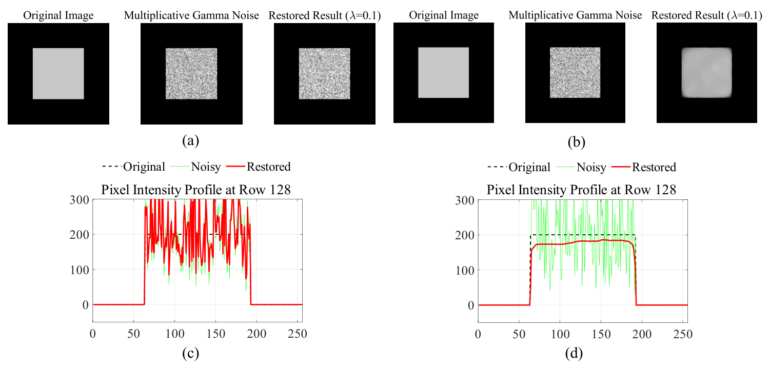
The improved TV algorithm demonstrates significant effectiveness on multiplicative noise, as shown in Figure 7. The improved algorithm can effectively handle noise perturbation while reconstructing a quasi-rectangular flat signal at the signal level, providing a clean foundation for subsequent edge filtering of SAR images.

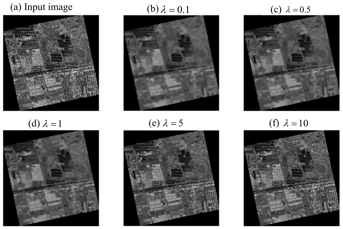
The regularisation parameter $\lambda$ in Equation (10) directly controls the trade-off between smoothness and fidelity: small values let the total-variation term dominate, which suppresses speckle strongly but also oversmooths edges, while large values pull the solution toward the observation and leave residual speckle. Figure 8 visualises this trade-off on a representative SAR patch across $\lambda \in \{0.1,0.5,1,2,5\}$: for $\lambda \le 0.5$ salient edges are blurred together with the noise, whereas for $\lambda \ge 2$ speckle is clearly preserved in homogeneous regions. The setting $\lambda =1$ provides the best compromise between speckle suppression and edge preservation on our data and is therefore adopted as the default value in all subsequent experiments.

4.2. Multi-Level Cross-Modal Edge Filtering

In optical–SAR image registration, edges and structural information serve as the important foundation for achieving stable cross-modal matching. The SRF method models edge detection as a structured prediction problem of local image patches, capable of utilizing common local structural patterns within edge blocks, such as straight lines, parallel lines, and T-type and Y-type intersections.

In the random forest framework, let the input sample be image patch $\mathit{x}$ with corresponding structured label $\mathit{y}$. The t-th decision tree at node j uses a binary split function $h(\mathit{x},{\mathit{\theta }}_j)$ to recursively partition samples. For the sample set $S_j$ at node j, the information gain can be written as:

$$∆H\left(S_j\right)=H\left(S_j\right)-\sum _{c\in \{L,R\}}{\displaystyle \frac{|S_j^c|}{|S_j|}}H\left(S_j^c\right)$$

(13)

where $H(·)$ denotes the node impurity measure (e.g., entropy). During testing, each tree outputs a local structured prediction at its leaf node, and the overall forest output is obtained by averaging across all trees:

$$\widehat{\mathit{y}}={\displaystyle \frac{1}{T}}{\displaystyle \sum _{t=1}^T}{\widehat{\mathit{y}}}_t$$

(14)

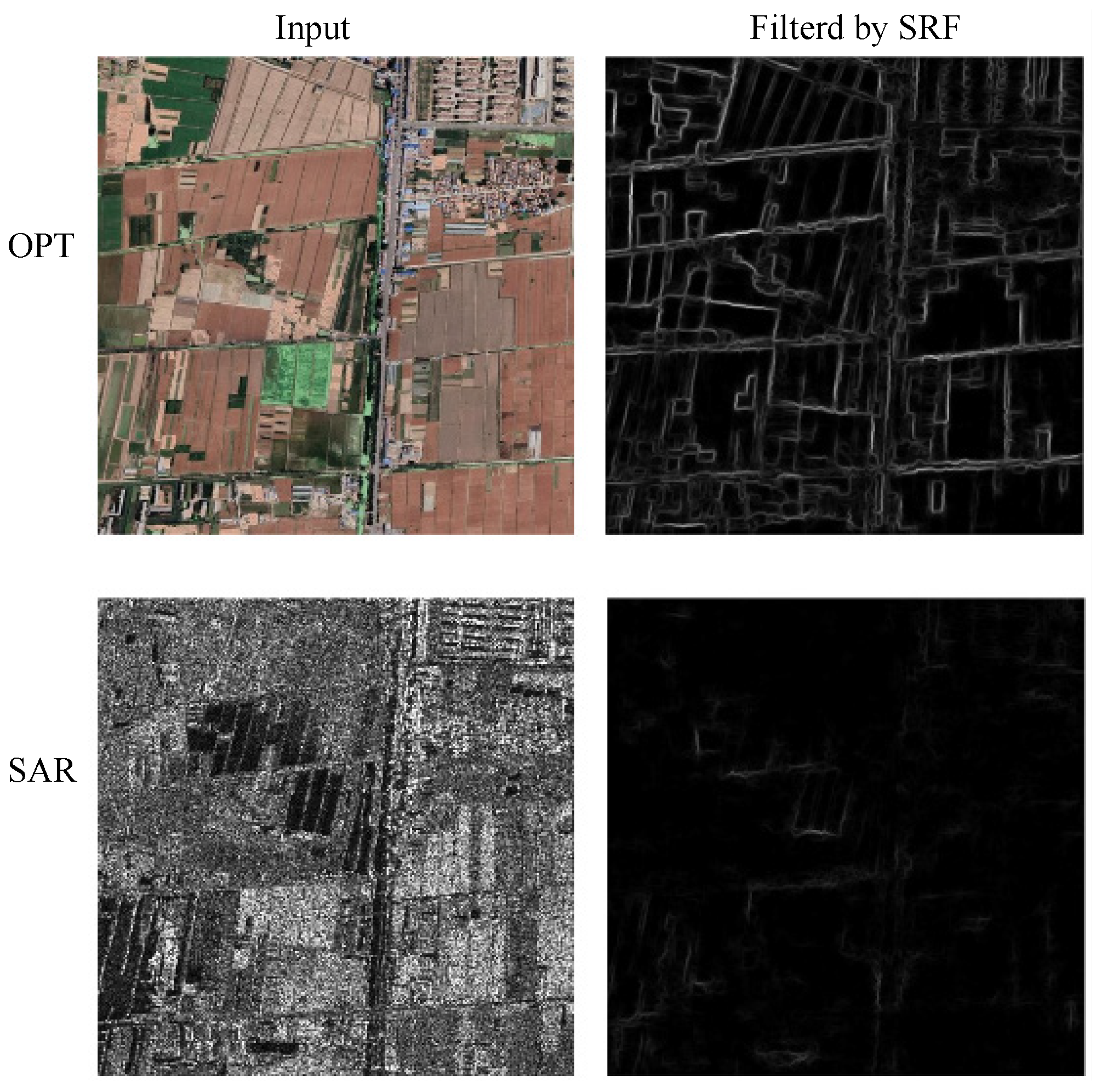
where T is the number of decision trees in the forest. However, SRF is designed for optical modality and requires adaptation for other modalities, as shown in Figure 9. This paper employs the phase congruency filter to reduce the modal difference of SAR images and improve the applicability of SRF.

Phase congruency is a feature based on multi-scale, multi-orientation wavelet analysis that maintains stable responses under intensity scaling, contrast changes, and modal differences. Let the image responses after convolution with even-symmetric filter ${\mathit{M}}_n^o$ and odd-symmetric filter ${\mathit{H}}_n^o$ at scale n and orientation o be:

$${\mathbf{e}}_{no}=\mathit{I}\ast {\mathit{M}}_n^o,{\mathbf{o}}_{no}=\mathit{I}\ast {\mathit{H}}_n^o$$

(15)

At each scale and orientation, the local amplitude and phase are defined as:

$$A_{no}=\sqrt{e_{no}^2+o_{no}^2},{\varphi }_{no}=atan2(o_{no},e_{no})$$

(16)

Combining all scales and orientations with noise compensation, the 2D phase congruency model is defined as:

$$PC\left(x\right)={\displaystyle \frac{{\sum }_o{W}_o⌊{\sum }_n{A}_{no}∆{\Phi }_{no}-T_o⌋}{{\sum }_o{\sum }_n{A}_{no}+\epsilon }}$$

(17)

where $W_o$ is the scale-orientation weight function, $\epsilon$ is a small constant to prevent division by zero, $\lfloor ·\rfloor$ is the truncation operator, and $∆{\Phi }_{no}$ is the phase deviation function. The normalized even-symmetric and odd-symmetric components across all scales and orientations are:

$$E_o=\sum _n{e}_{no},O_o=\sum _n{o}_{no}$$

(18)

For anisotropic characterization, moment analysis is applied to the phase congruency map. Let ${PC}_o$ be the phase congruency response at orientation o, then three intermediate quantities are computed:

$$a=\sum _o{PC}_o{cos}^2{\theta }_o,b=2\sum _o{PC}_{o}cos{\theta }_{o}sin{\theta }_o,c=\sum _o{PC}_o{sin}^2{\theta }_o$$

(19)

The principal axis direction, minimum moment, and maximum moment are then:

$${\theta }_p={\displaystyle \frac{1}{2}}atan2(b,a-c)$$

(20)

$$m={\displaystyle \frac{1}{2}}\left(a+c-\sqrt{b^2+{(a-c)}^2}\right),M={\displaystyle \frac{1}{2}}\left(a+c+\sqrt{b^2+{(a-c)}^2}\right)$$

(21)

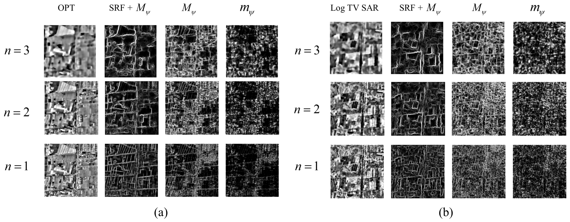
Experimental results show that the maximum moment response primarily corresponds to edge regions in the image, while the minimum moment response tends to characterize corner-like locally salient structures. The two provide complementary information for feature detection.

This paper fuses the advantages of the phase congruency filter and the SRF edge detector. The phase congruency filter enhances stable edge structures with cross-modal consistency, while the SRF algorithm further suppresses noise and fine-grained texture interference within the maximum moment space. Through their synergistic effect, clearer, more stable, and more consistent cross-modal edge responses can be obtained, as illustrated in Figure 10.

4.3. Keypoint Detection

4.3.1. Blob and Corner Detection

In cross-modal registration tasks, the keypoint detection stage is typically built upon edge filtering results, extracting locally salient structures at edge intersections as candidate keypoints. This paper extracts two types of keypoints.

The rationale for simultaneously extracting both blob and corner features lies in their complementary characteristics. Corner features [62] offer high localization accuracy and computational efficiency, yet they are sensitive to noise and exhibit limited scale robustness. In contrast, blob features [63], detected via scale-space extrema such as the Laplacian of Gaussian or nonlinear diffusion operators, provide stronger scale invariance and greater robustness to radiometric variations, albeit with relatively lower spatial localization precision. In optical–SAR cross-modal registration, these two feature types complement each other: corner keypoints supply precise geometric constraints, while blob keypoints contribute robust correspondences under significant scale and radiometric discrepancies. Combining both types yields higher matching density, enhanced robustness, and improved stability of the geometric transformation estimation.

First, the KAZE algorithm [64] is used to extract blob features, such as bright spots, dark spots, or local texture clusters, whose centers are typically local extrema. Coordinate deduplication and spatial non-maximum suppression (retaining only the point with the maximum response within the neighborhood) are performed to obtain a spatially uniform and response-stable final blob keypoint set.

In addition, a corner detection branch is constructed to supplement the response to high-curvature structures. Let the grayscale scale-space image at the l-th scale level be ${\mathit{I}}_l$, which is first linearly stretched and normalized. A tunable Gaussian filter is applied for smoothing:

$${\mathit{C}}_l={\mathit{G}}_{{\sigma }_c}\ast {\mathit{I}}_l$$

(22)

where ∗ denotes 2D convolution and ${\mathit{G}}_{{\sigma }_c}$ is a two-dimensional Gaussian kernel defined as

$${\mathit{G}}_{{\sigma }_c}(x,y)={\displaystyle \frac{1}{2\pi {\sigma }_c^2}}exp\left(-{\displaystyle \frac{x^2+y^2}{2{\sigma }_c^2}}\right)$$

(23)

with ${\sigma }_c$ controlling the degree of smoothing. To highlight high-curvature structures, a first-order Sobel filter is applied to obtain the gradient $\nabla {\mathit{C}}_l$, followed by a second-order Sobel filter on the gradient magnitude. The two directional filter templates are:

$${\mathit{S}}_x=\left[\begin{array}{ccc}-1& 0& 1\\ -2& 0& 2\\ -1& 0& 1\end{array}\right],{\mathit{S}}_y=\left[\begin{array}{ccc}-1& -2& -1\\ 0& 0& 0\\ 1& 2& 1\end{array}\right]$$

(24)

The second-order gradient components and magnitude are computed as:

$${\mathit{G}}_{xx}={\mathit{S}}_x\ast |\nabla {\mathit{C}}_l|,{\mathit{G}}_{yy}={\mathit{S}}_y\ast |\nabla {\mathit{C}}_l|$$

(25)

$${\mathit{G}}_{\mathrm{corner}}=\sqrt{{\mathit{G}}_{xx}^2+{\mathit{G}}_{yy}^2}$$

(26)

where ${\mathit{G}}_{\mathrm{corner}}$ is the enhanced corner gradient magnitude map, which more effectively highlights high-curvature regions in the image. After feature point detection, non-maximum suppression (NMS) is adopted. The suppression is implemented with a fixed hyperparameter window size of 5 pixels. After detecting the two types of feature points, feature description and matching are carried out in two separate branches, and the correspondences produced by the blob and corner branches are then merged into a single global match set for final transformation estimation. Specifically, let ${\mathcal{M}}_{\mathrm{blob}}$ and ${\mathcal{M}}_{\mathrm{corner}}$ denote the correspondence sets obtained from blob and corner features, respectively. The final correspondence set and transformation estimate are expressed as

$$\begin{array}{cc}\hfill {\mathcal{M}}_{\mathrm{all}}& ={\mathcal{M}}_{\mathrm{blob}}\cup {\mathcal{M}}_{\mathrm{corner}},\hfill \end{array}$$

(27)

$$\begin{array}{cc}\hfill \widehat{\mathit{H}}& =error\left({\mathcal{M}}_{\mathrm{all}}\right),\hfill \end{array}$$

(28)

where $\widehat{\mathit{H}}$ is the single global transformation matrix estimated from the pooled correspondences. In other words, the two feature branches are matched separately, but no branch-specific transformation matrices are solved and fused; instead, FSC is applied once on the combined correspondence set to obtain a globally consistent model.

4.3.2. Dominant Orientation Assignment

Since keypoints exhibit different local gradient directions, a stable dominant orientation is assigned before matching to improve rotational consistency.

The proposed assignment combines an orientation histogram with an intensity-centroid direction. The histogram captures dominant local gradients, but in cross-modal patches it often contains several comparable peaks. The centroid direction is therefore used as a structural cue to stabilise peak selection.

For a keypoint at the l-th scale level with pixel coordinates $(x_0,y_0)$, the gradient magnitude m and orientation $\theta$ of each pixel within the neighborhood are precomputed. A Gaussian-weighted orientation histogram is constructed by weighting gradient magnitudes:

$$w_G(x,y)=exp\left(-{\displaystyle \frac{{(x-x_0)}^2+{(y-y_0)}^2}{2{\left(1.5{\sigma }_l\right)}^2}}\right)$$

(29)

A circular mask with radius r retains only pixels within the circle, and the final contribution weight of each pixel is:

$$w(x,y)=w_G(x,y)·\mathbb{I}\left({(x-x_0)}^2+{(y-y_0)}^2\le r^2\right)$$

(30)

The orientation is quantized into $n=36$ bins, forming an orientation histogram:

$$H\left(k\right)=\sum _{(x,y)}w(x,y)·m(x,y)·\delta \left[bin\left(\theta \right(x,y\left)\right)=k\right],k=0,1,\dots ,35$$

(31)

For stability, a circular smoothing similar to SIFT’s five-point smoothing is applied:

$$\overline{H}\left(k\right)={\displaystyle \frac{H(k-2)+4H(k-1)+6H\left(k\right)+4H(k+1)+H(k+2)}{16}}$$

(32)

An orientation bin is considered a candidate dominant orientation when it simultaneously satisfies extremum and threshold conditions:

$$\overline{H}\left(k\right)>\overline{H}(k-1)\mathrm{and}\overline{H}\left(k\right)>\overline{H}(k+1)\mathrm{and}\overline{H}\left(k\right)\ge 0.8·\underset{j}{max}\overline{H}\left(j\right)$$

(33)

Following the ORB algorithm [65], a centroid-based orientation estimate is further introduced. For a local image patch P with grayscale values $I(x,y)$, the total grayscale sum is:

$$m_{00}=\sum _{x,y}I(x,y)$$

(34)

The centroid coordinates and orientation are computed as:

$$m_{10}=\sum _{x,y}x·I(x,y),m_{01}=\sum _{x,y}y·I(x,y)$$

(35)

$${\theta }_c=atan2(m_{01},m_{10})$$

(36)

Let ${\mathcal{B}}_{\mathrm{hist}}$ denote the set of significant histogram bins and let $b_c=bin\left({\theta }_c\right)$ be the bin index of the centroid direction. The final orientation is selected according to the number of significant histogram peaks:

$$\Theta =\left\{\begin{array}{cc}\left\{{\theta }_{\mathrm{hist},1}\right\},\hfill & |{\mathcal{B}}_{\mathrm{hist}}|=1,\hfill \\ \{{\theta }_{\mathrm{hist},i}\mid bin\left({\theta }_{\mathrm{hist},i}\right)\in {\mathcal{B}}_{\mathrm{hist}}\cap \left\{b_c\right\}\},\hfill & |{\mathcal{B}}_{\mathrm{hist}}|>1\mathrm{and}{\mathcal{B}}_{\mathrm{hist}}\cap \left\{b_c\right\}\ne ⌀,\hfill \\ \left\{{\theta }_c\right\},\hfill & |{\mathcal{B}}_{\mathrm{hist}}|>1\mathrm{and}{\mathcal{B}}_{\mathrm{hist}}\cap \left\{b_c\right\}=⌀.\hfill \end{array}\right.$$

(37)

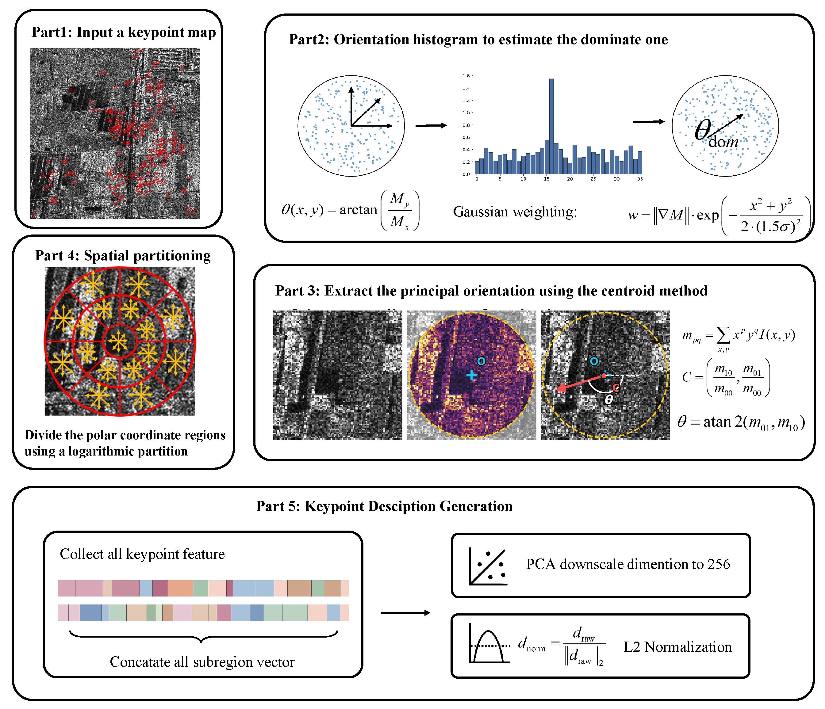
where ${\theta }_{\mathrm{hist},i}$ are the significant peaks of the orientation histogram and ${\theta }_c$ is the centroid-based direction. In practice, if the histogram contains only one significant peak, that peak is directly adopted as the final orientation. When multiple significant peaks exist, the centroid direction is used as an additional structural constraint, and only the intersection between the histogram-peak bin set and the centroid-direction bin is retained. This rule helps suppress the ambiguity caused by multiple comparable peaks while preserving both gradient saliency and structural consistency. If the intersection is empty, the centroid direction is used as a fallback. The subsequent descriptor uses the selected orientation for rotation alignment. The overall workflow is summarised in Figure 11.

4.4. Feature Description and Matching

In registration algorithms, detected keypoints require high-dimensional characterization through feature descriptors. Descriptors should maintain good properties including rotation invariance, distinctiveness, and robustness to illumination changes. This paper adopts the classic GLOH (Gradient Location–Orientation Histogram) descriptor [66], which demonstrates excellent stability.

For improved rotational consistency, the descriptor space is designed as a circular region divided into three radial levels and angular sectors, forming 17 spatial bins in total. Within each bin, GLOH quantizes local gradient orientations into $B=16$ direction bins. Gradient magnitudes of all pixels within each spatial region are accumulated into corresponding direction bins using trilinear interpolation. Concatenating the orientation histograms of all 17 spatial regions yields the original GLOH descriptor with dimension $17\times 16=272$.

However, the 272-dimensional original feature vector has high dimensionality with strong correlations between adjacent spatial and directional bins. To improve computational efficiency, PCA is introduced for dimensionality reduction and normalization.

For feature matching, this paper employs the FSC (Fast Sample Consensus) algorithm. Compared to RANSAC, the core idea of FSC is to progressively refine model parameters through an iterative consensus mechanism rather than immediately discarding the current model after each sampling and retaining only the highest-scoring candidate.

Let the minimum sample size be p (for affine transformation, $p=3$). First, p non-collinear matching point pairs are randomly sampled from the candidate set $\mathcal{M}$ to solve for the initial transformation matrix using least squares, obtaining the initial model ${\mathit{H}}^{\left(0\right)}$. The iterative consensus stage then begins. At the k-th iteration with current model ${\mathit{H}}^{\left(k\right)}$, the projection residual for each candidate matching pair is computed:

$$r_i^{\left(k\right)}={∥{\mathit{p}}_i^{\prime }-{\mathit{H}}^{\left(k\right)}{\mathit{p}}_i∥}_2$$

(38)

Given a distance threshold $\tau$, the current iteration’s inlier set is constructed:

$${\mathcal{I}}^{\left(k\right)}=\left\{i\in \{1,\dots ,N\}\mid r_i^{\left(k\right)}<\tau \right\}$$

(39)

The transformation model is then re-estimated only on the inlier set through least-squares optimization:

$${\mathit{H}}^{(k+1)}=arg\underset{\mathit{H}}{min}\sum _{i\in {\mathcal{I}}^{\left(k\right)}}{∥{\mathit{p}}_i^{\prime }-\mathit{H}{\mathit{p}}_i∥}_2^2$$

(40)

The above steps alternate until convergence or the maximum number of iterations is reached. Convergence is characterized by constraining the change between consecutive inlier sets below a threshold:

$$|{\mathcal{I}}^{(k+1)}▵{\mathcal{I}}^{\left(k\right)}|\le ϵ$$

(41)

where $|·|$ denotes set cardinality and ∆ denotes symmetric difference. When this condition is satisfied, the final geometric transformation estimate ${\mathit{H}}^{(k+1)}$ is output for precise alignment of the SAR image to the optical image coordinate system.

5. Results

5.1. Evaluation Metrics

The algorithm is comprehensively evaluated from four dimensions: registration accuracy, computational efficiency, the number of effective matches, and registration success rate. For each test image pair, each method first outputs its keypoint matching results (candidate correspondence set) and estimates a predicted transformation matrix $\widehat{\mathit{H}}$; the ground-truth transformation matrix is denoted as ${\mathit{H}}^{\ast }$.

Let a method obtain N matching point pairs on an image pair, with source image coordinates denoted as ${\mathit{p}}_i$. The ground-truth and predicted transformations map points to the target coordinate system:

$${\mathit{q}}_i^{\ast }=\mathcal{N}\left({\mathit{H}}^{\ast }{\tilde{\mathit{p}}}_i\right),{\widehat{\mathit{q}}}_i=\mathcal{N}\left(\widehat{\mathit{H}}{\tilde{\mathit{p}}}_i\right)$$

(42)

where ${\tilde{\mathit{p}}}_i$ is the homogeneous coordinate and $\mathcal{N}(·)$ is the homogeneous normalization operator. The point-wise geometric error is defined as:

$$e_i={∥{\mathit{q}}_i^{\ast }-{\widehat{\mathit{q}}}_i∥}_2$$

(43)

For the Number of Correct Matches (NCM), a threshold $\tau =5$ pixels is used to filter inliers:

$$\mathrm{NCM}=\left|\right\{i:e_i<\tau \left\}\right|$$

(44)

The Correct Match Ratio (CMR) further normalises NCM by the number of extracted feature points, providing a scale-independent measure of matching quality:

$$\mathrm{CMR}={\displaystyle \frac{N_{\mathrm{correct}}}{N}}$$

(45)

where $N_{\mathrm{correct}}$ corresponds to the NCM defined above, and N denotes the number of extracted feature points. In the experiments of this paper, N is set to the top 5000 feature points with the highest response values for all methods, and CMR is reported as a percentage.

To additionally measure robustness at the image-pair level, we report the success rate $\gamma$, defined as the percentage of test pairs whose final registration error satisfies a preset success threshold ${\tau }_s$:

$$\gamma ={\displaystyle \frac{1}{M}}{\displaystyle \sum _{j=1}^M}\mathbb{I}({\mathrm{RMSE}}_j<{\tau }_s)\times 100\%$$

(46)

where $\mathbb{I}(·)$ is the indicator function, ${\mathrm{RMSE}}_j$ is the registration error of the j-th test pair, and the success threshold is fixed at ${\tau }_s=4$ pixels in this work. When the test set contains M image pairs, the reported NCM, RMSE, and time are averages over all pairs, while CMR and success rate are reported as percentages.

5.2. Algorithm Effectiveness and Performance

All experiments were conducted on a Windows 11 workstation equipped with an AMD Ryzen 7 7735H CPU (Advanced Micro Devices, Inc., Santa Clara, CA, USA) and an NVIDIA GeForce RTX 4060 Laptop GPU (NVIDIA Corporation, Santa Clara, CA, USA), and GPU acceleration was enabled throughout the experiments. The algorithms were implemented in Matlab R2023a version. For FSC, the maximum number of iterations was set to 10,000, and the inlier threshold was fixed at 3 pixels. For all experiments, the Log-TV denoising strength and the number of Log-TV iterations are set to 1.0 and 50, respectively. The GLOH descriptor radius is fixed at 48. The base Gaussian scale is set to 1.6, with an inter-scale ratio of $2^{1/3}$ across three octaves. The image pyramid scaling factor (also used as the back-projection upsampling factor) is set to 1.6, and the initial Gaussian smoothing window size is 5. Quantitative testing was conducted on the validation set of the self-constructed optical–SAR registration dataset (denoted as HT dataset). The results are shown in

Table 3. Performance comparison of different algorithms on the self-constructed HT dataset. ↑ indicates that higher values are better, and ↓ indicates that lower values are better. Bold values denote the best result in each column.

Category	Method	Avg. RMSE ↓	Avg. NCM ↑	CMR (%) ↑	Succ. Rate $\mathit{\gamma }$ (%) ↑	Time (s) ↓
hand-crafted	3MRS	18.084	2.102	0.042	7.200	2.656
	LNIFT	7.781	3.680	0.074	62.500	0.768
	MS-HLMO	14.210	8.340	0.167	16.900	165.589
	RIFT	9.089	6.720	0.134	68.200	93.250
	OS-SIFT	15.071	2.404	0.048	4.600	7.430
	SRIF	3.907	6.528	0.131	83.600	10.907
Deep Learning	Matching Anything	1.869	193.450	3.869	100.000	15.003
	MapGlue	2.273	210.400	4.208	89.300	1.362
Ours	Ours	1.882	68.185	1.363	100.000	36.218

. For a fair comparison, the learning-based baselines Matching Anything and MapGlue are evaluated directly with their official pretrained weights in a zero-shot setting on the HT dataset and other benchmarks, without retraining or fine-tuning.

Specifically, 16 representative optical–SAR image pairs were sampled from the constructed dataset to form the validation set. To evaluate the stability and generalisation ability of the compared methods under realistic geometric perturbations, each pair was subjected to a random affine transformation, in which the scaling factor was randomly sampled from the range 0.8–1.2 and the rotation angle was randomly sampled from $-{90}^{°}$ to $+{90}^{°}$. The transformed pairs were then used to build the evaluation set for model performance assessment, which serves as the basis for the subsequent algorithm comparison, robustness analysis, and comprehensive performance testing.

On the HT dataset, the proposed method achieves the lowest RMSE (1.882) among the hand-crafted keypoint-based methods while also obtaining the highest NCM (68.185), the highest CMR (1.363), and a 100% success rate. These results indicate a favorable balance between geometric accuracy, effective correspondence quantity, and overall robustness. Since the proposed algorithm adopts a more complex filter structure and additionally involves SAR image preprocessing, its time cost is much higher than that of LNIFT with a relatively simple structure. Nevertheless, it achieves a higher matching success rate and better robustness. Among the learning-based baselines, Matching Anything yields a slightly lower RMSE, whereas MapGlue attains higher NCM and CMR values.

The higher NCM and CMR values of the learning-based methods mainly reflect their dense correspondence generation capability. Trained on large-scale data with strong matching priors, they tend to produce more candidate matches and higher recall, especially in texture-rich regions, which directly increases correspondence-count-based metrics.By contrast, the proposed hand-crafted pipeline emphasizes explicit structural consistency and geometric reliability, so it intentionally produces fewer but more stable correspondences. This trade-off is appropriate for training-free deployment under severe domain shifts, where transparent control of the preprocessing, detection, and matching stages is often more important than maximizing match density alone.

In terms of computational efficiency, the average time of the proposed method, while not the smallest, remains within an acceptable range. On the HT dataset, the total runtime is approximately 36.218 s. Within this total, the construction of the multi-scale filtering space takes about 9.87 s, and the extraction of blob and corner features takes about 15.91 s in total, which account for the main portion of the computational cost. These stages are the principal bottlenecks because they repeatedly evaluate multi-scale responses and process high-resolution slices in two feature branches. Compared with computationally expensive methods such as MS-HLMO and RIFT, the proposed method significantly improves registration accuracy and the number of inlier matches while maintaining good overall efficiency.

Several practical optimization strategies could further reduce runtime without changing the overall framework. First, the Log-TV preprocessing and multi-scale filtering stages can be accelerated by GPU implementation or multithreaded parallelisation. Second, the scale-space responses can be cached and reused between the blob and corner branches to avoid redundant filtering. Third, low-texture regions can be pruned earlier so that keypoint detection is performed only on candidate areas with sufficient structural information. Finally, approximate nearest-neighbour search and parallel consensus updates can accelerate matching and FSC estimation. These measures are expected to improve efficiency while preserving the accuracy advantage of the current design.

To avoid dataset bias affecting the evaluation, supplementary experiments were conducted on the widely recognized public OSdataset. Specifically, we adopt the validation set provided by ReDFeat [19], which is a curated subset of the OSdataset. As shown in

Table 4. Performance comparison on the OSdataset. ↑ indicates that higher values are better, and ↓ indicates that lower values are better. Bold values denote the best result in each column.

Category	Method	Avg. RMSE ↓	Avg. NCM ↑	CMR (%) ↑	Succ. Rate $\mathit{\gamma }$ (%) ↑	Time (s) ↓
hand-crafted	3MRS	2.802	220.132	4.440	63.200	0.923
	LNIFT	2.393	33.450	0.669	100.000	0.718
	MS-HLMO	6.012	10.582	2.512	34.500	0.720
	RIFT	4.317	12.723	0.255	64.900	30.260
	OS-SIFT	9.146	14.274	0.286	22.500	2.556
	SRIF	2.181	119.556	2.391	92.300	10.965
Deep Learning	Matching Anything	1.984	373.283	7.466	100.000	13.923
	MapGlue	3.473	206.012	4.120	100.000	1.563
Ours	Ours	2.015	47.235	1.180	100.000	22.295

, on this dataset the proposed method achieves the lowest RMSE (2.015) among the hand-crafted keypoint-based methods while maintaining a 100% success rate, further demonstrating good generalization capability and stable registration performance across different datasets.

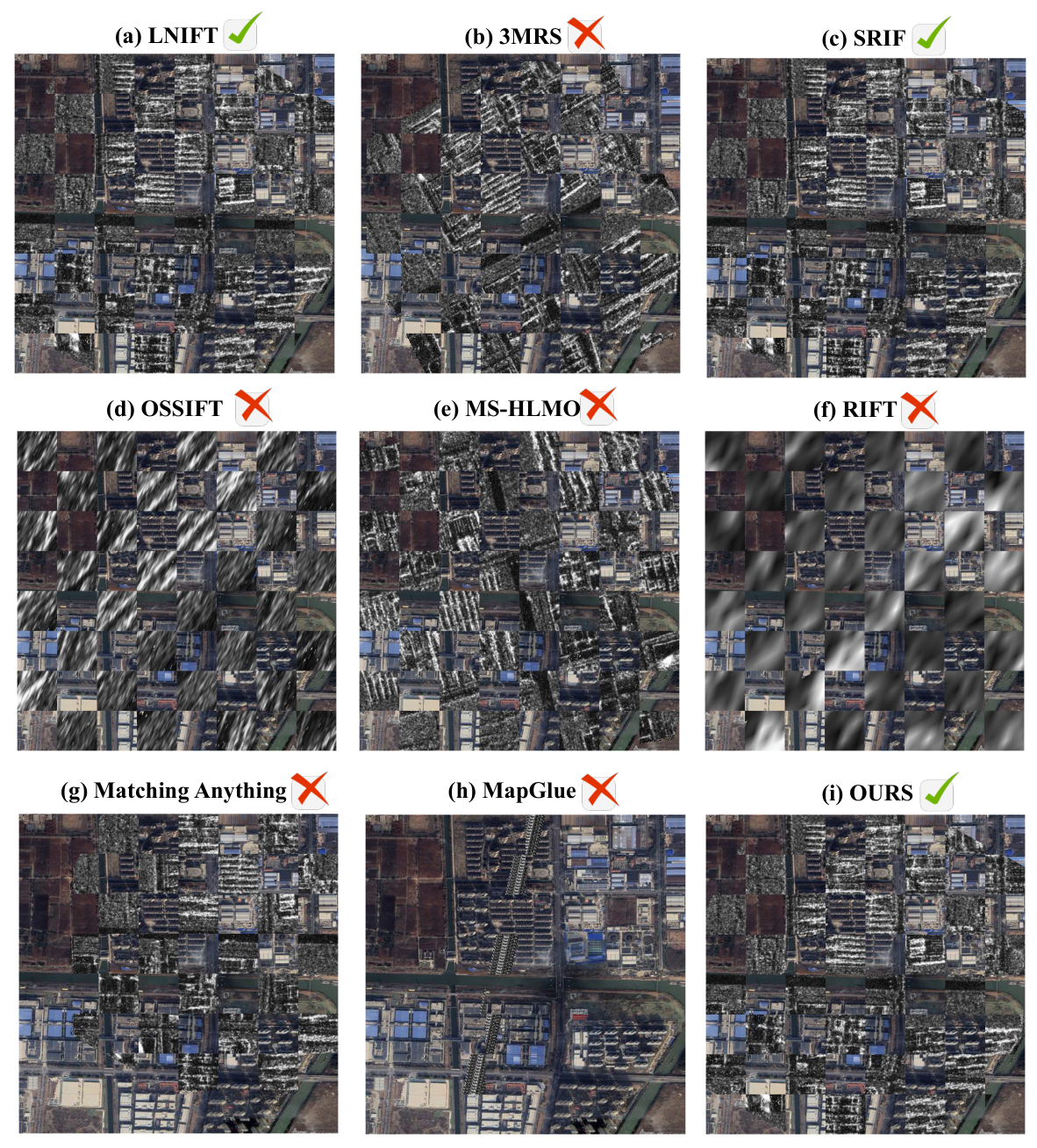
The proposed method maintains superior performance among hand-crafted keypoint-based methods across different datasets, validating the effectiveness of the multi-level edge filtering strategy and hybrid keypoint detection method. In qualitative terms, its correspondences are more spatially uniform and the checkerboard overlays preserve linear structures more continuously, which is consistent with the quantitative advantage in RMSE and success rate. By enhancing cross-modal shared structural information and improving keypoint extraction stability, the overall registration performance is significantly improved. Meanwhile, the average running time of 22.295 s maintains acceptable computational cost while achieving high registration accuracy and strong matching robustness.

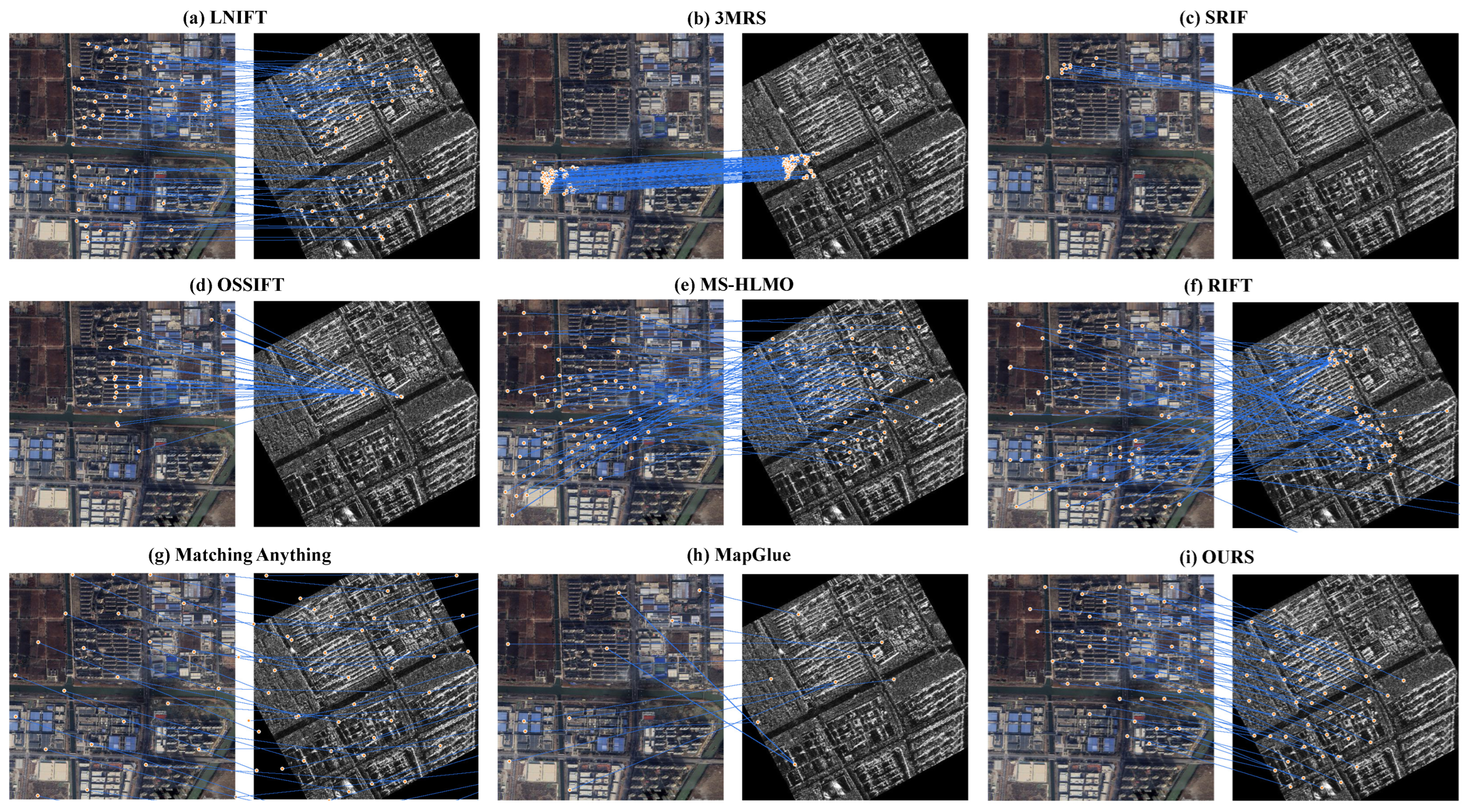
Compared with the hand-crafted baselines, the proposed method yields correspondences that are spatially more uniform and more widely distributed across the scene, with markedly fewer cross-image outlier links. This visual evidence is consistent with, and further reinforces, the higher NCM and lower RMSE reported in Table 3.

For further evaluating the generalization ability of the proposed method on different public datasets, quantitative results on the SAR2Opt dataset are additionally reported here. The corresponding table follows the same format and metrics as Table 3 to enable a consistent comparison.

As shown in

Table 5. Performance comparison of different algorithms on the SAR2Opt dataset. ↑ indicates that higher values are better, and ↓ indicates that lower values are better. Bold values denote the best result in each column.

Category	Method	Avg. RMSE ↓	Avg. NCM ↑	CMR (%) ↑	Succ. Rate $\mathit{\gamma }$ (%) ↑	Time (s) ↓
hand-crafted	3MRS	2.039	321.920	6.438	62.350	1.024
	LNIFT	2.039	33.421	0.668	100.000	0.643
	MS-HLMO	5.821	11.274	0.225	12.720	0.872
	RIFT	4.821	12.652	0.253	32.760	32.356
	OS-SIFT	10.233	14.231	0.284	23.250	2.621
	SRIF	1.981	107.702	2.154	94.200	11.242
Deep Learning	Matching Anything	1.923	327.251	6.545	100.000	6.231
	MapGlue	1.819	220.217	4.440	30.000	1.189
Ours	Ours	1.821	77.423	1.548	100.000	33.512

, on the SAR2Opt dataset the proposed method achieves the lowest RMSE (1.821) among the hand-crafted keypoint-based methods while maintaining a 100% success rate. Meanwhile, Matching Anything and MapGlue still perform more strongly on match-count-related metrics, which is consistent with the data-driven dense matching nature of these methods under zero-shot evaluation.

5.3. Robustness Tests

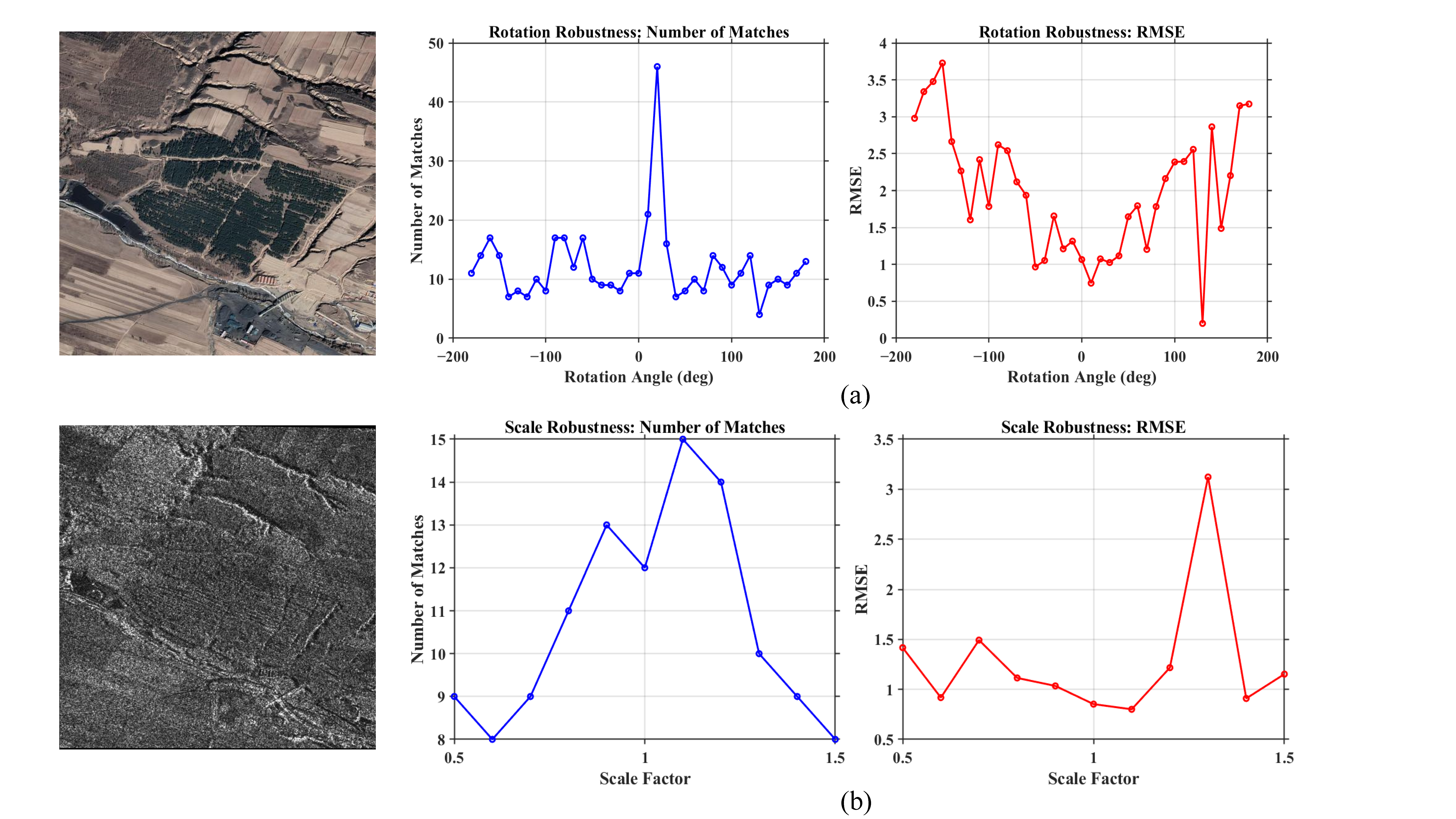
Robustness testing focused on two aspects: rotation invariance and scale invariance. Image pairs were randomly selected from the HT dataset to test registration performance under different rotation angles and scaling ratios, evaluated using the number of matching points and RMSE.

For scale invariance testing, the experimental results in Figure 12a show that within a moderate scaling range, the algorithm’s RMSE consistently remains at a low level. Within the 0.8–1.2 range, the RMSE even achieves sub-pixel level, and the number of effective matching points remains above 7, maintaining good robustness.

For rotation invariance testing, Figure 12b shows that at small rotation angles, the algorithm maintains a high number of matching points and low RMSE. When the rotation angle increases sharply, the number of matching points and RMSE decrease rapidly, but the number of matching points remains above 4, and the inlier RMSE hovers around 3, indicating that the algorithm still possesses strong robustness under rotational transformations. This validates the effectiveness of the rotationally invariant GLOH feature descriptor.

5.4. Ablation Study: SAR Image Preprocessing

To validate the effectiveness of the improved SAR-specific noise filtering strategy, ablation experiments were conducted on both the HT dataset, OSdataset and Sar2Opt, comparing results with and without the Log-TV preprocessing step. The results are shown in

Table 6. Performance comparison before and after SAR image preprocessing improvement. ↑ indicates that higher values are better, and ↓ indicates that lower values are better.

Dataset	Setting	Avg. Matches ↑	Avg. RMSE ↓	Avg. Time (s)
HT	w/o preprocessing	10.17	2.314	32.00
	w/preprocessing	68.18	1.882	34.06
OSdataset	w/o preprocessing	48.23	2.207	22.298
	w/preprocessing	47.31	2.015	21.3308
SAR2Opt	w/o preprocessing	72.42	2.213	33.215
	w/preprocessing	69.92	1.827	32.328

.

The SAR-specific filtering improves the overall registration quality on both datasets. On HT, it increases the average number of matches from 10.17 to 68.23 and reduces the average RMSE from 2.314 to 1.882, with only a slight increase in runtime; on SAR2Opt, it further reduces the average RMSE from 2.213 to 1.827 while slightly reducing runtime.

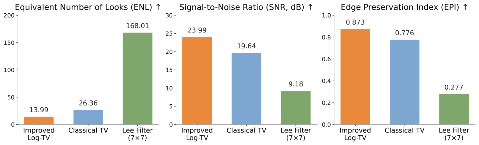
To further evaluate the denoising quality of the proposed Log-TV filter at the image level, we compare it against two widely used SAR despeckling baselines—the classical TV filter and the $7\times 7$ Lee filter—using three complementary image-quality metrics. The Equivalent Number of Looks (ENL) measures the smoothness of homogeneous regions and is defined as $\mathrm{ENL}={\mu }^2/{\sigma }^2$, where $\mu$ and $\sigma$ are the mean and standard deviation over a flat patch; a higher ENL indicates stronger speckle suppression and more uniform homogeneous regions. The Signal-to-Noise Ratio (SNR, in dB) reflects the overall fidelity of the denoised image with respect to the underlying clean signal, with larger values indicating better noise removal. The Edge Preservation Index (EPI) quantifies how well high-frequency structures (edges) are retained after filtering by comparing local gradient correlations between the filtered and reference images; values closer to 1 indicate stronger edge preservation.

It should be emphasised that ENL is inherently in conflict with the other two metrics: a larger ENL means that homogeneous regions are more uniform and speckle is more strongly suppressed, but such aggressive smoothing tends to blur edges as well, which in turn lowers SNR and EPI. ENL alone is therefore not a sufficient indicator of filter quality—it must be read together with SNR and EPI to judge whether a filter achieves a reasonable trade-off between speckle suppression and edge preservation. As shown in Figure 13, the Lee filter has the highest ENL ($168.01$) but the lowest SNR ($9.18$ dB) and EPI ($0.28$), a clear sign of over-smoothing, while classical TV lies in between ($26.36$/$19.64$ dB/$0.78$). The proposed Improved Log-TV filter keeps ENL at a reasonable $13.99$ yet achieves the best SNR ($23.99$ dB) and EPI ($0.87$), giving the most favourable trade-off between speckle suppression and edge preservation for downstream matching.

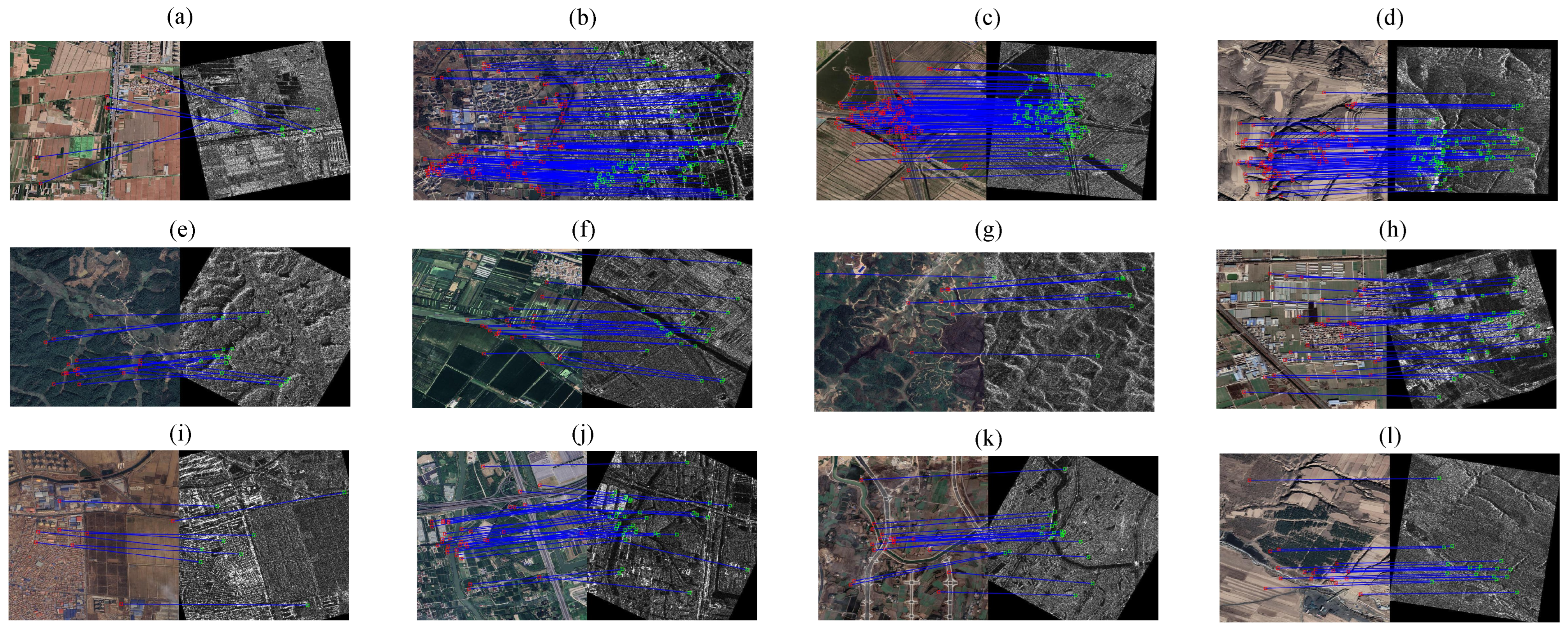
Beyond the quantitative metrics, the keypoint matching visualization provides an intuitive view of the registration quality. As shown in Figure 14, the correspondences established by the proposed method are highly consistent and clean: the matching lines connect semantically equivalent structures—such as road intersections, building corners, and field boundaries—across the optical and SAR tiles with very few crossing or outlier links, and the correspondences are spread over the entire scene rather than clustering in a small region. This visually consistent and outlier-free matching pattern corroborates the low RMSE and high success rate reported in the quantitative comparison, indicating that the hybrid keypoint detection together with the multi-level edge filtering produces stable and geometrically reliable correspondences under cross-modal differences.

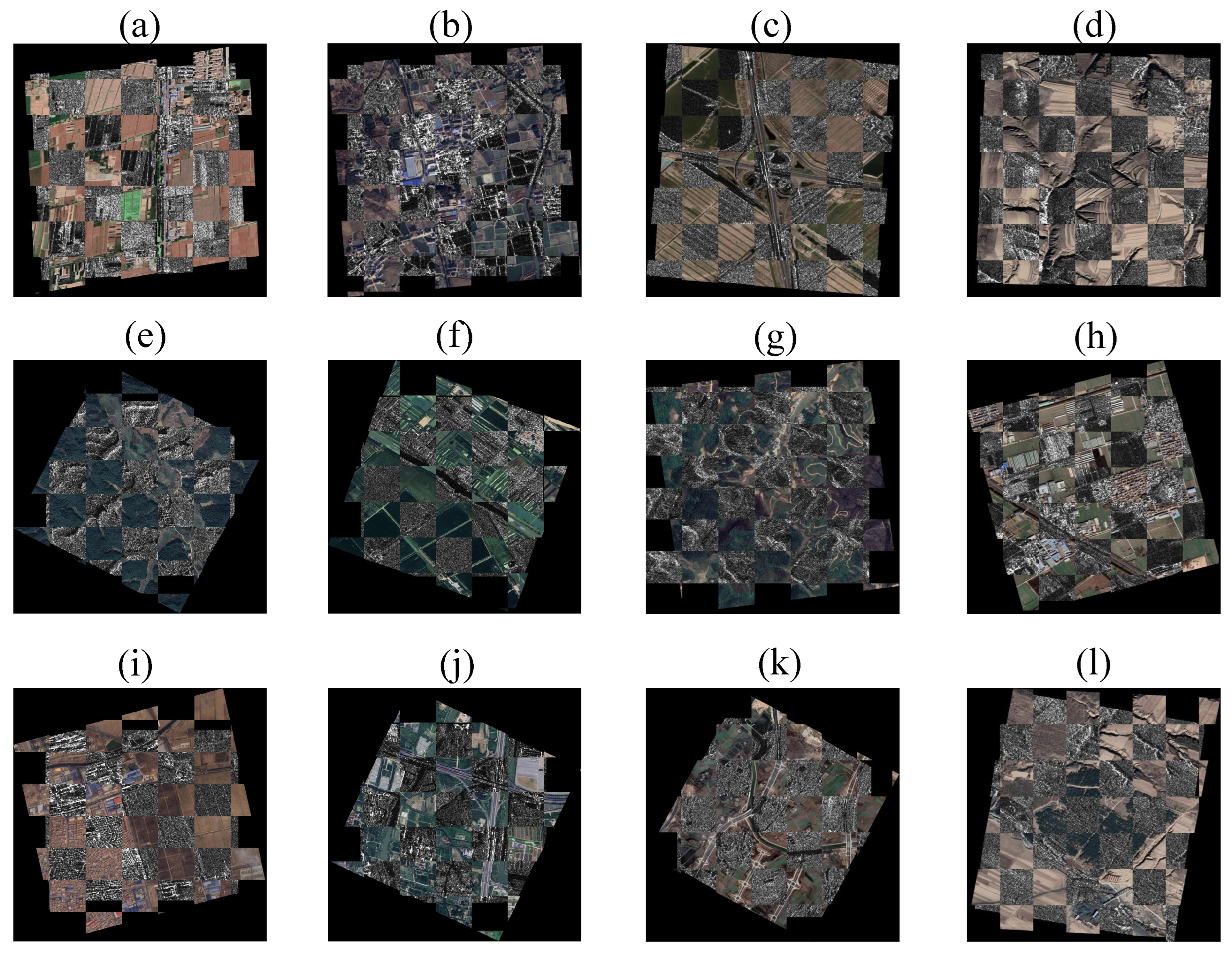
The checkerboard visualization in Figure 15 further confirms the alignment quality: linear structures such as roads, field boundaries and building outlines remain continuous when alternating between optical and SAR tiles, indicating sub-pixel-level geometric consistency after transformation estimation. The remaining artefacts are concentrated in regions where SAR-side speckle dominates fine texture, which is consistent with the observations reported in Section 5.4.

6. Discussion

The construction of the high-resolution optical–SAR registration dataset addresses a critical gap in the field. Compared to existing public datasets such as OSdataset (single-channel optical, 256 × 256), SEN12MS (10-m resolution), and QXS-SAROPT, the proposed HT dataset offers advantages in spatial resolution (3-m SAR/1-m optical), slice size (512 × 512), and scene diversity covering multiple terrain types across China. The multi-stage quality filtering pipeline, including high-frequency energy-based texture screening and VLM-assisted stitching artifact detection, ensures high data quality. Validation through registration metrics confirms that the dataset provides a solid foundation for algorithm development and evaluation.

The experimental results demonstrate strong comprehensive advantages of the proposed registration method among hand-crafted keypoint-based approaches across multiple evaluation metrics. Achieving the lowest RMSE together with consistently high success rates on multiple datasets indicates that the estimated transformation model is more consistent with the ground-truth transformation while preserving reliable registration stability. Qualitatively, the proposed method produces cleaner matches and more continuous structural alignment in the visual comparisons, suggesting that its advantage is perceptible beyond the metric values alone. This validates the effectiveness of the multi-level edge filtering strategy in enhancing cross-modal shared structural information. Although learning-based matchers such as Matching Anything and MapGlue can produce more matches, the proposed method offers a competitive training-free alternative with strong interpretability and cross-scene generalization.

The multi-level hybrid edge filtering strategy, which combines phase congruency analysis with structured random forest edge detection, effectively addresses two key challenges: the inadequacy of SRF when directly applied to SAR images, and the noise-sensitivity of phase congruency in SAR imagery. By operating within a Gaussian scale space, the framework ensures scale-invariant structural feature extraction.

The dual-branch keypoint detection scheme provides complementary structural representations through blob and corner features. The robust orientation assignment strategy, combining histogram-based and centroid-based methods, improves the stability of orientation estimation in cross-modal scenarios, directly benefiting the subsequent GLOH descriptor computation and matching reliability.

The ablation study shows that the Log-TV preprocessing step consistently reduces RMSE across HT, OSdataset, and SAR2Opt while keeping the computational overhead acceptable in practice. This indicates that the proposed preprocessing strategy provides a stable performance gain for cross-modal registration. The logarithmic domain transformation effectively converts the multiplicative noise problem into an additive one, enabling the classical TV framework to be applied to SAR denoising.

It should be noted that due to the relatively complex multi-scale filtering, hybrid edge enhancement, and multi-branch feature detection processes introduced in the front end, the computational overhead of the proposed method is relatively large. Future work should focus on lightweight design of the filtering module, efficient implementation of key steps, and computational optimization of the overall pipeline.

Figure 16 and Figure 17 are produced from the same optical–SAR image pair and provide complementary views of registration quality: the former visualises the keypoint correspondences directly, whereas the latter overlays the registered SAR image onto the optical image as a checkerboard so that residual misalignment shows up as breakage of linear features (roads, building outlines, field boundaries). The selected pair represents a typical complex-texture urban scene with densely interleaved buildings, roads and vegetation, and pronounced speckle on the SAR side—a stringent test of cross-modal registration reliability.

As shown in the checkerboard overlay (Figure 17), even under such cluttered urban texture, the proposed method preserves road and building outlines continuously across alternating tiles, indicating reliable sub-pixel-level alignment. Among the hand-crafted baselines, LNIFT and SRIF remain competitive on this scene as well: their checkerboard tile boundaries are visibly aligned. The remaining baselines (3MRS, MS-HLMO, RIFT, OS-SIFT) leave noticeable mis-registration along linear structures, which is consistent with the relative ordering of the proposed method, LNIFT and SRIF in Table 3.

7. Conclusions

This paper addresses the substantial modal differences and noise interference between optical and SAR images by constructing a large-scale, high-resolution registration dataset and proposing a cross-modal registration method within the hand-crafted keypoint paradigm, augmented with multi-level edge filtering. The main contributions and findings are summarized as follows:

• A large-scale, high-resolution optical–SAR registration dataset is constructed based on HongTu-1 satellite 3-m SAR imagery and Google Earth optical imagery at zoom level 17, covering diverse scenes across China. The standardized construction pipeline includes terrain correction, georeferencing, standardized slicing, and multi-stage quality filtering.
• An improved Log-TV denoising model is introduced for SAR image preprocessing, which effectively suppresses multiplicative speckle noise by transforming the problem to the logarithmic domain while preserving important edge structures.
• A multi-level hybrid edge filtering strategy combining phase congruency analysis and structured random forest edge detection is constructed within a Gaussian scale space. This strategy enhances stable geometric structural responses at different scales while suppressing noise and fine-grained pseudo-texture interference.
• A dual-branch feature detection framework integrating blob and corner features is designed, along with a coordinated orientation assignment strategy that incorporates both histogram-based peak detection and centroid-based orientation estimation, improving the consistency and reliability of feature descriptions and matching.
• Experimental results on the self-constructed high-resolution HT dataset, as well as on the public OSdataset and SAR2Opt benchmarks, demonstrate that the proposed method consistently achieves low RMSE and high success rates. It also maintains competitive computational efficiency and strong robustness to scale and rotation variations among hand-crafted methods.
• In practical deployment, the proposed method is well suited to training-free optical–SAR registration scenarios in which annotated data are limited and interpretability is required, such as dataset construction, geospatial mapping, and preprocessing for downstream change detection or multimodal fusion pipelines.

Future research directions include lightweight design of the filtering module, GPU-accelerated and parallel implementation of Log-TV preprocessing and multi-scale filtering, reuse of shared scale-space responses, early pruning of low-texture regions, and faster approximate matching and consensus estimation.

References

1. Zhou, Y.; Yang, X.; Zhang, G.; Wang, J.; Liu, Y.; Hou, L.; Jiang, X.; Liu, X.; Yan, J.; Lyu, C.; et al. Mmrotate: A rotated object detection benchmark using pytorch. In Proceedings of the 30th ACM International Conference on Multimedia, Lisbon, Portugal, 10–14 October 2022; pp. 7331–7334. [Google Scholar]
2. Yang, X.; Yan, J.; Feng, Z.; He, T. R3det: Refined single-stage detector with feature refinement for rotating object. In Proceedings of the AAAI Conference on Artificial Intelligence, Online, 2–9 February 2021; Volume 35, pp. 3163–3171. [Google Scholar]
3. Zhang, W.; Liu, X.; Liu, N.; Liu, M.; Liao, W.; Xu, C.; Yang, X. SPWOOD: Sparse Partial Weakly-Supervised Oriented Object Detection. arXiv 2026, arXiv:2602.03634. [Google Scholar] [CrossRef]
4. Yang, X.; Zhou, Y.; Zhang, G.; Yang, J.; Wang, W.; Yan, J.; Zhang, X.; Tian, Q. The KFIoU loss for rotated object detection. arXiv 2022, arXiv:2201.12558. [Google Scholar]
5. Yu, Y.; Yang, X.; Li, Q.; Zhou, Y.; Da, F.; Yan, J. H2RBox-v2: Incorporating symmetry for boosting horizontal box supervised oriented object detection. Adv. Neural Inf. Process. Syst. 2023, 36, 59137–59150. [Google Scholar]
6. Shi, Y.; Jia, H.; Teng, S.; Wang, H. Enhancing Dense Ship Detection in SAR Images Through Cluster-Region-Based Super-Resolution. IEEE J. Sel. Top. Appl. Earth Obs. Remote Sens. 2026, 19, 8478–8492. [Google Scholar] [CrossRef]
7. Zhang, T.; Zhang, X.; Zhu, P.; Tang, X.; Li, C.; Jiao, L.; Zhou, H. Semantic attention and scale complementary network for instance segmentation in remote sensing images. IEEE Trans. Cybern. 2021, 52, 10999–11013. [Google Scholar] [CrossRef] [PubMed]
8. Sharma, R.; Saqib, M.; Lin, C.T.; Blumenstein, M. A survey on object instance segmentation. SN Comput. Sci. 2022, 3, 499. [Google Scholar] [CrossRef]
9. Wen, Q.; Yang, J.; Yang, X.; Liang, K. Patchdct: Patch refinement for high quality instance segmentation. In Proceedings of the Eleventh International Conference on Learning Representations, Online, 25–29 April 2022. [Google Scholar]
10. Zhou, W.; Xie, W.; Kamata, S.i.; Hou, H.C.; Wong, M.S.; Wang, H. HSIseg: Progressively enhanced extensible multi-modality framework for large patch-wise hyperspectral image segmentation. Neurocomputing 2026, 667, 132261. [Google Scholar]
11. He, J.; Yuan, Q.; Li, J.; Xiao, Y.; Zhang, L. A self-supervised remote sensing image fusion framework with dual-stage self-learning and spectral super-resolution injection. ISPRS J. Photogramm. Remote Sens. 2023, 204, 131–144. [Google Scholar]
12. He, J.; Lin, L.; Zheng, Z.; Yuan, Q.; Li, J.; Zhang, L.; Zhu, X.X. Spatial-X fusion for multi-source satellite imageries. Remote Sens. Environ. 2026, 334, 115214. [Google Scholar]
13. Tewkesbury, A.P.; Comber, A.J.; Tate, N.J.; Lamb, A.; Fisher, P.F. A critical synthesis of remotely sensed optical image change detection techniques. Remote Sens. Environ. 2015, 160, 1–14. [Google Scholar] [CrossRef]
14. Cheng, G.; Huang, Y.; Li, X.; Lyu, S.; Xu, Z.; Zhao, H.; Zhao, Q.; Xiang, S. Change detection methods for remote sensing in the last decade: A comprehensive review. Remote Sens. 2024, 16, 2355. [Google Scholar] [CrossRef]
15. Li, W.; Li, Y.; Zhu, Y.; Wang, H. Unsupervised multitemporal SAR image change detection via foreground-background collaborative optimization. Int. J. Appl. Earth Obs. Geoinf. 2026, 146, 105008. [Google Scholar] [CrossRef]
16. Chen, H.; Song, J.; Han, C.; Xia, J.; Yokoya, N. ChangeMamba: Remote sensing change detection with spatiotemporal state space model. IEEE Trans. Geosci. Remote Sens. 2024, 62, 1–20. [Google Scholar] [CrossRef]
17. Chen, H.; Lan, C.; Song, J.; Ibañez, D.; Xia, J.; Schindler, K.; Yokoya, N. Multimodal remote sensing change detection: An image matching perspective. ISPRS J. Photogramm. Remote Sens. 2026, 233, 487–501. [Google Scholar] [CrossRef]
18. Lowe, D.G. Distinctive image features from scale-invariant keypoints. Int. J. Comput. Vis. 2004, 60, 91–110. [Google Scholar] [CrossRef]
19. Deng, Y.; Ma, J. ReDFeat: Recoupling detection and description for multimodal feature learning. IEEE Trans. Image Process. 2022, 32, 591–602. [Google Scholar] [CrossRef] [PubMed]
20. Cui, S.; Xu, M.; Ma, A.; Zhong, Y. Modality-free feature detector and descriptor for multimodal remote sensing image registration. Remote Sens. 2020, 12, 2937. [Google Scholar] [CrossRef]
21. Ryu, S.; Kim, S.; Sohn, K. LAT: Local area transform for cross modal correspondence matching. Pattern Recognit. 2017, 63, 218–228. [Google Scholar] [CrossRef]
22. Liu, X.; Lei, Z.; Yu, Q.; Zhang, X.; Shang, Y.; Hou, W. Multi-modal image matching based on local frequency information. EURASIP J. Adv. Signal Process. 2013, 2013, 3. [Google Scholar] [CrossRef]
23. Lin, H.; Yuan, X.; Yin, Y.; Fang, Z.; Wang, Z.; Cheng, L. BMSR: A multimodal image registration method for addressing modal differences and spatial misalignment. Infrared Phys. Technol. 2026, 155, 106484. [Google Scholar] [CrossRef]
24. Peng, T.; Zhou, L.; Lei, G.; Yang, P.; Ye, Y. Robust multimodal image matching based on radiation invariant phase correlation. ISPRS Ann. Photogramm. Remote Sens. Spat. Inf. Sci. 2024, 10, 309–316. [Google Scholar] [CrossRef]
25. Lee, J.S. Digital image enhancement and noise filtering by use of local statistics. IEEE Trans. Pattern Anal. Mach. Intell. 1980, 2, 165–168. [Google Scholar] [CrossRef]
26. Dellinger, F.; Delon, J.; Gousseau, Y.; Michel, J.; Tupin, F. SAR-SIFT: A SIFT-like algorithm for SAR images. IEEE Trans. Geosci. Remote Sens. 2014, 53, 453–466. [Google Scholar] [CrossRef]
27. Yu, Q.; Ni, D.; Jiang, Y.; Yan, Y.; An, J.; Sun, T. Universal SAR and optical image registration via a novel SIFT framework based on nonlinear diffusion and a polar spatial-frequency descriptor. ISPRS J. Photogramm. Remote Sens. 2021, 171, 1–17. [Google Scholar] [CrossRef]
28. Dollár, P.; Zitnick, C.L. Fast edge detection using structured forests. IEEE Trans. Pattern Anal. Mach. Intell. 2014, 37, 1558–1570. [Google Scholar] [CrossRef] [PubMed]
29. Kovesi, P. Phase Congruency Detects Corners and Edges. In Proceedings of the DICTA, Sydney, Australia, 10–12 December 2003; Volume 2003, pp. 309–318. [Google Scholar]
30. Xiang, Y.; Wang, F.; You, H. OS-SIFT: A robust SIFT-like algorithm for high-resolution optical-to-SAR image registration in suburban areas. IEEE Trans. Geosci. Remote Sens. 2018, 56, 3078–3090. [Google Scholar] [CrossRef]
31. Li, J.; Hu, Q.; Ai, M. RIFT: Multi-modal image matching based on radiation-variation insensitive feature transform. IEEE Trans. Image Process. 2019, 29, 3296–3310. [Google Scholar] [CrossRef]
32. Ye, Y.; Shen, L.; Hao, M.; Wang, J.; Xu, Z. Robust optical-to-SAR image matching based on shape properties. IEEE Geosci. Remote Sens. Lett. 2017, 14, 564–568. [Google Scholar] [CrossRef]
33. Li, J.; Xu, W.; Shi, P.; Zhang, Y.; Hu, Q. LNIFT: Locally normalized image for rotation invariant multimodal feature matching. IEEE Trans. Geosci. Remote Sens. 2022, 60, 1–14. [Google Scholar] [CrossRef]
34. Fan, Z.; Liu, Y.; Liu, Y.; Zhang, L.; Zhang, J.; Sun, Y.; Ai, H. 3MRS: An effective coarse-to-fine matching method for multimodal remote sensing imagery. Remote Sens. 2022, 14, 478. [Google Scholar] [CrossRef]
35. Google. Google Earth. 2026. Available online: https://earth.google.com/ (accessed on 10 May 2026).
36. Sommervold, O.; Gazzea, M.; Arghandeh, R. A survey on SAR and optical satellite image registration. Remote Sens. 2023, 15, 850. [Google Scholar] [CrossRef]
37. Li, B.; Guan, D.; Xie, Y.; Zheng, X.; Chen, Z.; Pan, L.; Zhao, W.; Xiang, D. Global optical and SAR image registration method based on local distortion division. Remote Sens. 2025, 17, 1642. [Google Scholar] [CrossRef]
38. Li, Z.; Zhang, H.; Huang, Y.; Li, H. A Robust Strategy for Large-Size Optical and SAR Image Registration. Remote Sens. 2022, 14, 3012. [Google Scholar] [CrossRef]
39. Fan, B.; Huo, C.; Pan, C.; Kong, Q. Registration of optical and SAR satellite images by exploring the spatial relationship of the improved SIFT. IEEE Geosci. Remote Sens. Lett. 2012, 10, 657–661. [Google Scholar] [CrossRef]
40. Fan, J.; Xiong, Q.; Li, J.; Liu, G.; Song, W. Multimodal image matching using phase congruency-based self-similarity structural features. In Proceedings of the 2022 17th International Conference on Control, Automation, Robotics and Vision (ICARCV); IEEE: Piscataway, NJ, USA, 2022; pp. 322–325. [Google Scholar]
41. Raguram, R.; Chum, O.; Pollefeys, M.; Matas, J.; Frahm, J.M. USAC: A universal framework for random sample consensus. IEEE Trans. Pattern Anal. Mach. Intell. 2012, 35, 2022–2038. [Google Scholar] [CrossRef]
42. Dalal, N.; Triggs, B. Histograms of oriented gradients for human detection. In Proceedings of the 2005 IEEE Computer Society Conference on Computer Vision and Pattern Recognition (CVPR’05); IEEE: Piscataway, NJ, USA, 2005; Volume 1, pp. 886–893. [Google Scholar]
43. Wan, G.; Ye, Z.; Xu, Y.; Huang, R.; Zhou, Y.; Xie, H.; Tong, X. Multimodal remote sensing image matching based on weighted structure saliency feature. IEEE Trans. Geosci. Remote Sens. 2023, 62, 1–16. [Google Scholar] [CrossRef]
44. Fischler, M.A.; Bolles, R.C. Random sample consensus: A paradigm for model fitting with applications to image analysis and automated cartography. Commun. ACM 1981, 24, 381–395. [Google Scholar] [CrossRef]
45. Wu, Y.; Ma, W.; Gong, M.; Su, L.; Jiao, L. A novel point-matching algorithm based on fast sample consensus for image registration. IEEE Geosci. Remote Sens. Lett. 2014, 12, 43–47. [Google Scholar] [CrossRef]
46. Sarlin, P.E.; DeTone, D.; Malisiewicz, T.; Rabinovich, A. Superglue: Learning feature matching with graph neural networks. In Proceedings of the IEEE/CVF Conference on Computer Vision and Pattern Recognition, Seattle, WA, USA, 13–19 June 2020; pp. 4938–4947. [Google Scholar]
47. Sun, J.; Shen, Z.; Wang, Y.; Bao, H.; Zhou, X. LoFTR: Detector-free local feature matching with transformers. In Proceedings of the IEEE/CVF Conference on Computer Vision and Pattern Recognition, Online, 19–25 June 2021; pp. 8922–8931. [Google Scholar]
48. Lindenberger, P.; Sarlin, P.E.; Pollefeys, M. Lightglue: Local feature matching at light speed. In Proceedings of the IEEE/CVF International Conference on Computer Vision, Paris, France, 1–6 October 2023; pp. 17627–17638. [Google Scholar]
49. Xiang, Y.; Tao, R.; Wang, F.; You, H.; Han, B. Automatic registration of optical and SAR images via improved phase congruency model. IEEE J. Sel. Top. Appl. Earth Obs. Remote Sens. 2020, 13, 5847–5861. [Google Scholar] [CrossRef]
50. Schmitt, M.; Hughes, L.H.; Qiu, C.; Zhu, X.X. SEN12MS–A curated dataset of georeferenced multi-spectral sentinel-1/2 imagery for deep learning and data fusion. arXiv 2019, arXiv:1906.07789. [Google Scholar] [CrossRef]
51. Huang, M.; Xu, Y.; Qian, L.; Shi, W.; Zhang, Y.; Bao, W.; Wang, N.; Liu, X.; Xiang, X. The QXS-SAROPT dataset for deep learning in SAR-optical data fusion. arXiv 2021, arXiv:2103.08259. [Google Scholar]
52. Zhao, Y.; Celik, T.; Liu, N.; Li, H.C. A Comparative Analysis of GAN-based Methods for SAR-to-Optical Image Translation. IEEE Geosci. Remote Sens. Lett. 2022, 19, 3512605. [Google Scholar] [CrossRef]
53. Wivell, C.E.; Steinwand, D.R.; Kelly, G.G.; Meyer, D.J. Evaluation of terrain models for the geocoding and terrain correction, of synthetic aperture radar (SAR) images. IEEE Trans. Geosci. Remote Sens. 1992, 30, 1137–1144. [Google Scholar] [CrossRef]
54. Loew, A.; Mauser, W. Generation of geometrically and radiometrically terrain corrected SAR image products. Remote Sens. Environ. 2007, 106, 337–349. [Google Scholar] [CrossRef]
55. Farr, T.G.; Rosen, P.A.; Caro, E.; Crippen, R.; Duren, R.; Hensley, S.; Kobrick, M.; Paller, M.; Rodriguez, E.; Roth, L.; et al. The shuttle radar topography mission. Rev. Geophys. 2007, 45, RG2004. [Google Scholar] [CrossRef]
56. Small, D. Flattening gamma: Radiometric terrain correction for SAR imagery. IEEE Trans. Geosci. Remote Sens. 2011, 49, 3081–3093. [Google Scholar] [CrossRef]
57. Flenniken, J.M.; Stuglik, S.; Iannone, B.V. Quantum GIS (QGIS): An introduction to a free alternative to more costly GIS platforms: FOR359/FR428, 2/2020. EDIS 2020, 2020, 7. [Google Scholar] [CrossRef]
58. Bai, S.; Cai, Y.; Chen, R.; Chen, K.; Chen, X.; Cheng, Z.; Deng, L.; Ding, W.; Gao, C.; Ge, C.; et al. Qwen3-vl technical report. arXiv 2025, arXiv:2511.21631. [Google Scholar] [CrossRef]
59. Ye, Y.; Shan, J.; Bruzzone, L.; Shen, L. Robust registration of multimodal remote sensing images based on structural similarity. IEEE Trans. Geosci. Remote Sens. 2017, 55, 2941–2958. [Google Scholar] [CrossRef]
60. Ye, Y.; Bruzzone, L.; Shan, J.; Bovolo, F.; Zhu, Q. Fast and robust matching for multimodal remote sensing image registration. IEEE Trans. Geosci. Remote Sens. 2019, 57, 9059–9070. [Google Scholar] [CrossRef]
61. Rudin, L.I.; Osher, S.; Fatemi, E. Nonlinear total variation based noise removal algorithms. Phys. D Nonlinear Phenom. 1992, 60, 259–268. [Google Scholar] [CrossRef]
62. Harris, C.; Stephens, M. A Combined Corner and Edge Detector. In Proceedings of the Alvey Vision Conference, Manchester, UK, 31 August–2 September 1988. [Google Scholar]
63. Lindeberg, T. Feature detection with automatic scale selection. Int. J. Comput. Vis. 1998, 30, 79–116. [Google Scholar] [CrossRef]
64. Alcantarilla, P.F.; Bartoli, A.; Davison, A.J. KAZE features. In Proceedings of the European Conference on Computer Vision; Springer: Berlin/Heidelberg, Germany, 2012; pp. 214–227. [Google Scholar]
65. Rublee, E.; Rabaud, V.; Konolige, K.; Bradski, G. ORB: An efficient alternative to SIFT or SURF. In Proceedings of the 2011 International Conference on Computer Vision; IEEE: Piscataway, NJ, USA, 2011; pp. 2564–2571. [Google Scholar]
66. Mikolajczyk, K.; Schmid, C. A performance evaluation of local descriptors. IEEE Trans. Pattern Anal. Mach. Intell. 2005, 27, 1615–1630. [Google Scholar] [CrossRef]
Figure 1. Example of an image pair from our self-constructed dataset, shown as cropped subregions of the full-scene data. (a): Google Earth optical imagery at zoom level 17, with multi-temporal stitching seams clearly visible; (b): terrain-corrected 3-m resolution SAR image from the HongTu-1 satellite, exhibiting characteristic speckle noise.
Remotesensing 18 01741 g001
Figure 2. Heatmap of the spatial distribution of full-scene sampling locations. The horizontal axis denotes longitude, the vertical axis denotes latitude, and darker colors indicate a larger number of samples in the corresponding region.
Remotesensing 18 01741 g002
Figure 3. Dataset construction pipeline overview. The process includes full-scene pairing via geographic coordinates, SAR Preprocessing Chain, geometric registration refinement, and standardized slicing with quality filtering.
Remotesensing 18 01741 g003
Figure 4. High-frequency energy distribution of dataset slices. The bimodal pattern clearly separates texture-rich regions (right peak) from featureless black-border areas (left peak), enabling effective threshold-based filtering.
Remotesensing 18 01741 g004
Figure 5. Sub-figures (al) are randomly sampled preview pairs from our self-constructed dataset, which will serve as the validation set in subsequent experiments. In each sub-figure, the left tile is the SAR image and the right tile is the optical image.
Remotesensing 18 01741 g005
Figure 6. Overall pipeline of the proposed registration method. Stage 1 applies improved Log-TV denoising. Stage 2 extracts hierarchical edge pyramids with SRF filtering and phase congruency detection. Stage 3 detects blob and corner keypoints and generates 256-dimensional descriptors via PCA. Stage 4 matches features and estimates the transformation matrix with FSC.
Remotesensing 18 01741 g006
Figure 7. Comparison of TV and Log-TV denoising on multiplicative Gamma noise ( L = 4 , λ = 0.1 ). (a) Denoising result of the TV algorithm on the square region corrupted by Gamma noise. (b) Denoising result of the Log-TV algorithm on the same noisy square region. (c) Row-128 intensity profile before and after denoising with the TV algorithm. (d) Row-128 intensity profile before and after denoising with the Log-TV algorithm. It can be seen that Log-TV effectively eliminates the perturbations introduced by noise.
Remotesensing 18 01741 g007
Figure 8. Sub-figures (af) illustrate the effect of the regularisation parameter λ in the Log-TV model. Small λ oversmooths structural edges together with speckle, while large λ leaves residual speckle in homogeneous regions. The setting λ = 1 balances the two effects and is adopted as the default in this work.
Remotesensing 18 01741 g008
Figure 9. Comparison of SRF edge detection on optical and SAR images. On optical images the SRF filter extracts clean and well-localised edge responses, whereas on SAR images–due to the very different intensity distribution and the heavy speckle noise–SRF fails to produce coherent edge responses, motivating the modality-aware adaptation introduced in this section.
Remotesensing 18 01741 g009
Figure 10. Effect of the proposed hybrid edge filter on the two modalities. Panel (a) shows optical images, and panel (b) shows SAR images preprocessed by Log-TV. Within each panel, the columns show the input image at different scales, the hybrid response, the phase congruency maximum-moment response, and the phase congruency minimum-moment response.
Remotesensing 18 01741 g010
Figure 11. Pipeline of the proposed dominant orientation assignment, combining a Gaussian-weighted gradient orientation histogram with the ORB-style intensity-centroid direction to form the final orientation set Θ .
Remotesensing 18 01741 g011
Figure 12. Robustness analysis under scale and rotation transformations in a chosen pair. (a) Scale robustness analysis. (b) Rotation robustness analysis.
Remotesensing 18 01741 g012
Figure 13. Filter ablation on SAR despeckling. Comparison of the proposed Improved Log-TV filter, the classical TV filter and the 7 × 7 Lee filter in terms of Equivalent Number of Looks (ENL), Signal-to-Noise Ratio (SNR) and Edge Preservation Index (EPI). Higher SNR and EPI indicate better fidelity and edge preservation; an extremely high ENL accompanied by a low EPI reflects over-smoothing rather than superior denoising.
Remotesensing 18 01741 g013
Figure 14. Sub-figures (al) show the keypoint matching visualization results on a subset of the HT dataset test set.
Remotesensing 18 01741 g014
Figure 15. Sub-figures (al) show the checkerboard visualization of registration results on a subset of the HT dataset test set.
Remotesensing 18 01741 g015
Figure 16. Sub-figures (ai) show the visual comparison of matching results on representative HT pairs. The proposed method yields more uniformly distributed correspondences and fewer outlier links than the hand-crafted baselines, consistent with Table 3.
Remotesensing 18 01741 g016
Figure 17. Sub-figures (ai) show the checkerboard overlay of the same pair as in Figure 16. Continuous linear structures across alternating tiles indicate reliable sub-pixel alignment. The proposed method, LNIFT, and SRIF preserve structure continuity, while 3MRS, MS-HLMO, RIFT, and OS-SIFT show clear misalignment.
Remotesensing 18 01741 g017