Benchmarking Object Detection and a Novel Self-Supervised Framework for Weed Detection in Soybean

Highlights

What are the main findings?

• Across eight object detectors, YOLO models led on accuracy and computational cost, while two-stage detectors achieved the highest threshold-independent weed coverage (WCR-AUC).
• GeoCLR, a self-supervised framework pretrained on unlabeled aerial imagery, produced more class-discriminative features than ImageNet pretraining and recovered roughly 95% of full-data detection accuracy using only half of the annotations.

What are the implications of the main findings?

• Detector selection for precision spraying should be based on operational and deployment metrics in addition to mAP, as the weed detector solely relying on accuracy may not provide highest spraying efficacy or the lowest deployment cost.
• Self-supervised pretraining on unlabeled UAS imagery can substantially reduce the annotation effort needed to field a usable weed detector, improving scalability across fields and seasons.

Abstract

Palmer amaranth is one of the most problematic weeds in soybean production in the United States and can cause major yield loss if not managed early. This study benchmarked eight object detection models for site-specific Palmer amaranth detection in soybean using high-resolution uncrewed aerial system (UAS) imagery, with the goal of supporting targeted herbicide application and reducing herbicide usage. The models YOLOv8m, YOLOv9m, YOLOv10m, YOLOv11m, Faster R-CNN, RetinaNet, RT-DETR, and a self-supervised Faster R-CNN variant were evaluated using five-fold cross-validation on 2064 annotated aerial RGB image tiles containing 5990 bounding-box instances across multiple growth stages and field conditions, with an additional 7615 unlabeled tiles used for self-supervised pretraining. All detectors followed an identical 150-epoch schedule with early stopping and were compared using Friedman with Iman–Davenport correction and post hoc Nemenyi tests. Detectors were assessed on three axes: detection accuracy (mAP and class-wise AP), operational spraying efficacy summarized by a threshold-independent weed coverage rate area under the curve (WCR-AUC), and computational deployment cost across batch sizes from 1 to 32. The YOLO models achieved the highest detection accuracy along with the lowest inference latency and memory use but showed weaker threshold-independent weed coverage; the two-stage Faster R-CNN models showed the opposite pattern. Weighing all three axes, YOLOv8m provided the most practical balance for real-time deployment. The study also introduced GeoCLR, a self-supervised pretraining framework that constructs positive pairs from UAS flight overlap rather than synthetic augmentation. GeoCLR produced more structured and class-discriminative features than ImageNet pretraining, and a detector fine-tuned on only half of the annotations recovered approximately 95% of full-data accuracy. Together, these results highlight the importance of operational metrics for practical model selection and show that self-supervised pretraining can reduce annotation effort for scalable precision agriculture.

1. Introduction

Weeds interfere with crop growth and compete for soil nutrients, water, light, and space [1]. Weeds have the potential to reduce soybean (Glycine max (L.) Merr.) crop yield by 26–29% globally [2]. It has been estimated that weed infestations in soybean result in an annual revenue loss of $16.2 billion in the United States (U.S.) [3]. Following the widespread adoption of genetically modified herbicide-resistant crops, herbicides became the most commonly used tool by growers to manage weeds. However, various research studies have highlighted the negative impact of herbicides on groundwater quality, human health, and the environment [4,5,6,7]. Furthermore, the problem of herbicide-resistant weeds is becoming more prevalent, making it difficult for growers to manage weeds efficiently and effectively [8,9,10]. According to a survey conducted by the Weed Science Society of America (WSSA) in 2022, Palmer amaranth (Amaranthus palmeri S. Watson) has been recognized as number one among the seven most troublesome weeds in soybean crop in the U.S. [11]. It has been found that early emerging Palmer amaranth can have a more negative impact on the crop yield than those that emerge when the crop is fully grown [12]. The presence of just eight Palmer amaranth weeds per meter of row can cause soybean yield loss of up to 78% [13]. Therefore, it is crucial for growers to monitor the Palmer amaranth densities in their fields right from the beginning of crop plantation to design the most effective weed management strategies and implement them at the right time to reduce crop yield loss. Even when herbicides are sprayed early, Palmer amaranth plants that escape control or emerge later in the season can cause significant yield loss; hence, detection at multiple growth stages is also essential.

Herbicides are traditionally applied using agricultural boom sprayers; however, that approach results in the wastage of herbicides due to uniform spread even in those areas where weeds are absent. Recently, site-specific weed control (SSWC) measures have gained popularity in effectively controlling weeds. The SSWC focuses on targeting only those areas where weeds are present in the field and thus reducing herbicide usage [14,15]. Building SSWC tools require a comprehensive understanding of weed densities in the fields [16]. Several factors such as similarities in color, texture, and shape between crops and weeds, different lighting conditions, and the growth stage of the crops and weeds can affect the performance of SSWC tools in precisely locating the locations of the weeds in the large field [17].

The early years of computer vision weed detection research date back to the 1990s and relied on manual feature extraction based on color, texture, and shape by weed science experts [18,19,20,21]. Classical machine learning methods such as artificial neural networks, support vector machines, and random forests achieved good accuracy in this setting [22,23,24], but generalize poorly to natural field conditions and required expert-driven feature design [25,26]. Convolutional neural networks (CNNs) have since become the standard deep-learning approach for agricultural image analysis [27,28,29,30,31,32,33,34]. However, CNN classification models treat an entire image as a single class, while uncrewed aerial system (UAS) and ground robotic platforms commonly capture multiple weed and crop species in a single frame. Object detection algorithms such as You Only Look Once (YOLO) address this by localizing multiple instances within an image [35,36,37].

CNN-based algorithms require large amounts of annotated data to train robust weed detection models. The quality and diversity of training imagery strongly influence model performance and depend on factors such as sensor type, acquisition platform (e.g., UAS, robots, handheld cameras), weather conditions, illumination, and field variability [38,39]. Previous studies have used RGB imagery collected from handheld cameras and UAS platforms for Palmer amaranth detection in cotton and soybean. For example, a previous study achieved 76.9% mAP@0.5 using YOLOv5n for detecting carpetweed (Mollugo verticillata L.), morning glory (Ipomoea spp.), and Palmer amaranth in cotton [36]. Similarly, another study trained YOLOv5 on handheld and aerial imagery for Palmer amaranth detection in soybean and reported 77% mAP@0.5 [40]. Although YOLO-based models are the most widely used object detection algorithms for weed recognition, their evaluation in agriculture has often been limited to relatively small or controlled datasets and usually focused on a single generation such as YOLOv3 or YOLOv5. Since then, newer YOLO versions (YOLOv8 to YOLOv11) have introduced architectural and training modifications intended to improve both detection accuracy and computational efficiency. However, newer architectures do not necessarily perform better under real aerial field conditions [41]. In addition, other detector families such as Faster R-CNN, RetinaNet, and transformer-based detectors follow substantially different localization and feature-representation strategies [42,43,44,45]. Evaluating these detector families together therefore provides a broader understanding of how single-stage, two-stage, and transformer-based architectures behave under aerial agricultural imaging conditions. However, no study has systematically compared recent YOLO generations alongside other major detector families on high-resolution UAS imagery of Palmer amaranth in soybean across diverse growth stages and field environments.

Developing robust object detection models for SSWC requires large volumes of expert-annotated bounding boxes, making dataset generation both time-intensive and expensive, particularly when expanding across new fields, weed species, or growing seasons. Self-supervised learning (SSL) offers an alternative approach in which visual representations are learned directly from unlabeled imagery and later transferred to downstream tasks using relatively small labeled datasets [46,47]. Existing SSL frameworks such as SimCLR [46], MoCo [48], and Seasonal Contrast (SeCo) [49] have shown that meaningful image representations can be learned either from augmentation-based views or from naturally occurring spatial and temporal relationships. These hypotheses are particularly relevant for UAS-based agricultural imaging because overlapping flight trajectories naturally provide multiple views of the same physical field region under slight variation in viewing angle, illumination, and acquisition conditions. However, the use of UAS flight-overlap geometry as a positive-pair signal for self-supervised pretraining in aerial weed detection has not been systematically explored.

Beyond standard object detection metrics, a weed detection model should also be evaluated based on how useful it is for site-specific spraying. Metrics such as mAP@0.5 and mAP@0.5:0.95 are useful for measuring detection accuracy and localization quality, but they do not directly show how many weeds would actually be sprayed or how much herbicide could be saved. Previous studies have proposed deployment-oriented metrics such as weed coverage rate and area sprayed to evaluate precision spraying performance [50]; however, these metrics have generally been reported only at a single fixed confidence threshold, which does not capture detector behavior across the full operating range used in commercial spot-spraying systems [51]. Computational deployment characteristics such as inference latency at multiple batch sizes, throughput, model size, and GPU memory have similarly been under-reported, despite being decisive for on-board UAS deployment. Together, these gaps in operational and deployment reporting limit how directly current weed detector benchmarks translate into field-deployment guidance for UAS-based precision spraying.

The present study addresses these gaps through three methodological contributions. First, a novel self-supervised pretraining framework that constructs positive pairs from the natural spatial overlap between adjacent UAS images within a flight, rather than from synthetic augmentations of a single image, is introduced. Second, a threshold-independent operational metric is introduced to summarize weed-targeting performance across the full range of confidence thresholds rather than at a single operating point. Third, a three-axis evaluation framework combining detection accuracy, operational spraying behavior, and computational deployment cost is used to compare detector architectures jointly, rather than along a single criterion. To our knowledge, benchmarking recent YOLO variants alongside Faster R-CNN, RetinaNet, and a transformer-based detector within this framework on UAS imagery of Palmer amaranth in soybean has not been reported in the precision spraying literature.

The current study was designed using data collected from U.S. soybean production fields in the Mid-Atlantic region with the following three objectives:

1.

Develop an annotated Palmer amaranth and soybean image dataset representative of diverse weather conditions and growth stages.

2.

Benchmark recent YOLO models (v8–v11) alongside Faster R-CNN, RetinaNet, and a transformer-based detector using an evaluation framework spanning detection accuracy, operational spraying efficacy, and computational deployment cost.

3.

Introduce a self-supervised pretraining framework that learns from unlabeled UAS imagery, and evaluate its label efficiency for downstream Palmer amaranth detection in soybean.

2. Materials and Methods

2.1. Data Acquisition

The research study was conducted at the Eastern Shore Agricultural Research and Extension Center, Painter, Virginia (37.58566°N, 75.78511°W). Soybean for this experiment was planted in two different fields on 17 June 2022, using the Enlist E3^® (Corteva Agriscience, Indianapolis, IN, USA) variety at a seeding rate of 140,000 seeds per acre. The experiment included three weed density treatments—low (5 m⁻²), medium (10 m⁻²), and high (20 m⁻²)—along with a weed-free control. These densities were created by spreading Palmer amaranth seeds within plots and thinning them to the desired density to allow variation in plant growth, overlap, and competition with soybean. To maintain Palmer amaranth presence, grasses were selectively controlled using clethodim (Select Max^®, Valent USA LLC, Walnut Creek, CA, USA), while other broadleaf weeds were removed manually. The experiment followed a randomized complete block design (RCBD) with four replications. Each treatment plot measured 12 m in width and 3.7 m in length, with a 1 m border on all sides. The goal of this experimental design was to introduce variability in weed density and field conditions so that the collected aerial imagery represents realistic scenarios for model development and deployment.

RGB images of soybean and Palmer amaranth were collected at different crop development stages, where soybean image data was collected through multiple flights at vegetative stages (V2–V5 and V6–V8), and reproductive stages (R1–R3 and R5–R8). Palmer amaranth image data was collected, starting from 7.5 cm tall seedlings to approximately 75 cm. Apart from the two structured experimental fields, separate fields containing only soybean and natural infestations of Palmer amaranth without soybean were also imaged to capture pure class representations. These additional datasets were collected across two growing seasons (2022 and 2023).

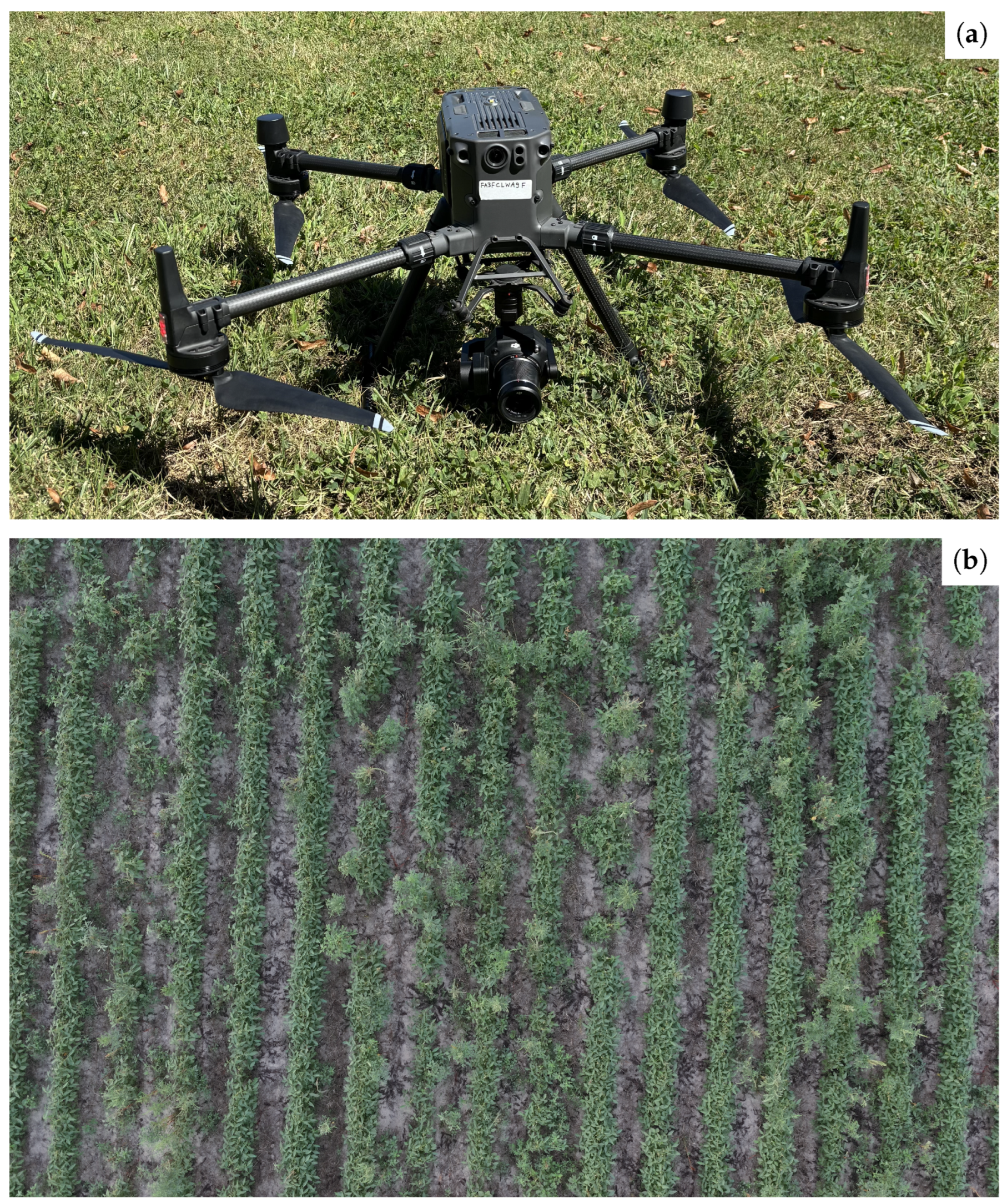
Data were collected using a Zenmuse P1 camera (focal length 0.035 m) mounted on a DJI Matrice-300 UAS (DJI, Shenzhen, China). The drone was flown at a height of 12 m with a constant horizontal speed of 5.6 km/h. The ground sampling distance of the grid flight plan was 0.15 cm/pixel, with side and frontal overlap ratios of 70% and 80%, respectively. The total area covered in one complete flight was 3030 m², with an average flight time of 14 min. Flights were conducted between 9:00 am and 3:00 pm to ensure good lighting conditions. The average wind speed during flights was 4.8 km/h. A total of 16,589 RGB images were collected across the growing seasons. Each raw image had a resolution of $8192\times 5460$ pixels. The DJI Matrice-300 UAS with the Zenmuse P1 camera, along with a representative raw RGB image of a soybean field infested with Palmer amaranth, are shown in Figure 1.

2.2. Image Processing and Annotation

The original aerial RGB images had a resolution of $8192\times 5460$ pixels, which was too large to be directly processed during model training. To address this issue, image tiles of $640\times 640$ pixels were extracted using Python version 3.8.16 and the Pillow library (version 9.5.0). Tiles were generated using a non-overlapping sliding-window approach starting from the top-left corner of each raw image, producing a fixed grid of patches per image. 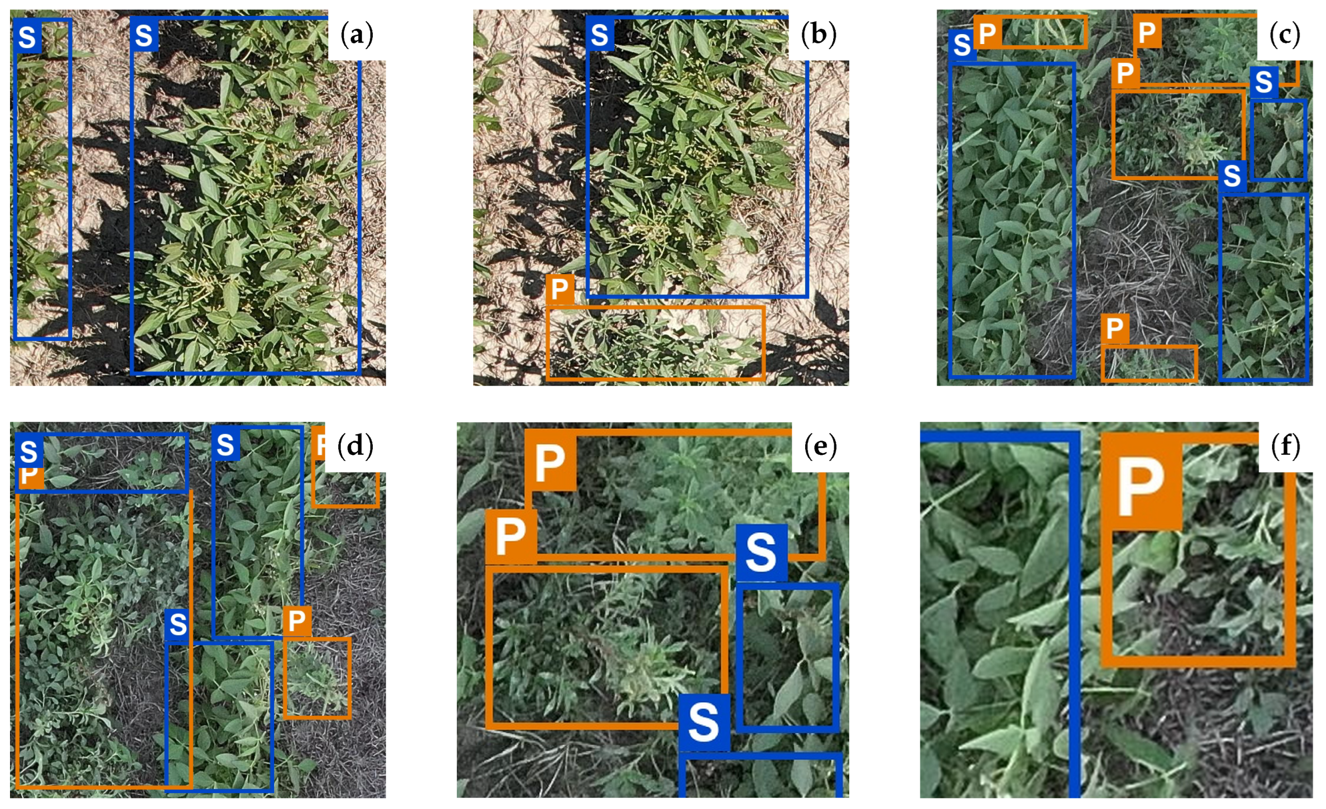For object detection training, the extracted tiles were manually annotated using LabelImg (https://github.com/heartexlabs/labelImg, accessed on 13 May 2026). A total of 2064 images were labeled with rectangular bounding boxes around soybean and Palmer amaranth plants. During annotation, images with poor visual quality or unclear plant features were excluded. The final dataset captured diversity in lighting conditions, backgrounds, plant densities, and growth stages, as illustrated in Figure 2. In total, 5990 bounding box instances were annotated, including 4513 Palmer amaranth and 1477 soybean objects. The dataset included variation in Palmer amaranth morphology across growth stages and densities, whereas soybean generally exhibited more consistent visual structure. The original YOLO annotations were converted to COCO JSON format to ensure compatibility with Faster R-CNN, RetinaNet, and RT-DETR. Using a unified annotation format ensured that all object detection models were trained and evaluated under identical conditions for fair benchmarking.

To characterize the visual properties of the annotated classes, all 5990 bounding-box instances were analyzed for object size and color distribution. Soybean instances were generally larger than Palmer amaranth instances, with a median bounding-box area of 67,417 px² compared to 40,209 px² for Palmer amaranth (Mann–Whitney U, $p=5.6\times {10}^{-24}$). Soybean foliage also showed a higher excess-green index than Palmer amaranth (39.8 vs. 30.1; Mann–Whitney U, $p<{10}^{-190}$), indicating stronger contrast against the soil background.

A separate set of 1523 raw aerial images that were not part of the object detection dataset was used for SSL pretraining. From each raw image, five $640\times 640$ tiles were extracted using flight-metadata-driven sampling (described in Section 2.4), resulting in a total of 7615 unlabeled images for SSL training. These unlabeled images were used to construct positive pairs for contrastive learning. To evaluate the quality of SSL-learned representations for plant species classification, an independent labeled dataset consisting of 468 images (216 soybean and 252 Palmer amaranth) was used as a held-out test set. This classification dataset was fully separated from both the SSL pretraining data and the object detection annotation dataset, ensuring that no image appeared in more than one experimental pipeline.

2.3. Object Detection Networks

Eight object detection models were evaluated in this study: four single-stage anchor-free YOLO detectors (YOLOv8m, YOLOv9m, YOLOv10m, and YOLOv11m), a single-stage anchor-based detector (RetinaNet), a two-stage anchor-based detector (Faster R-CNN), a real-time transformer-based detector (RT-DETR), and a Faster R-CNN model initialized using the SSL framework described in Section 2.4 (Faster R-CNN-GeoCLR). These models represent different object detection approaches, including anchor-based, anchor-free, two-stage, transformer-based, and SSL-initialized detection frameworks. All models were trained and evaluated on the same aerial Palmer amaranth and soybean dataset to compare how model architecture and pretraining strategy influence detection accuracy, inference speed, trainability, and deployment performance.

2.3.1. YOLO

YOLO is a single-stage object detection model that divides an image into grids, where each grid predicts bounding box coordinates, objectness confidence, and class probabilities in a single forward pass. The model uses three main loss components: bounding box regression loss, objectness loss, and classification loss. Non-Maximum Suppression (NMS) is generally used to remove redundant detections based on IoU thresholds. Unlike earlier YOLO versions that relied on predefined anchor boxes, YOLOv8 through YOLOv11 use an anchor-free detection approach. However, YOLOv10 is an NMS-free training strategy designed to reduce post-processing overhead during inference [52]. Each YOLO version is available in five model sizes—nano, small, medium, large, and extra-large—allowing trade-offs between accuracy, computational cost, and inference speed. In this study, the medium variants of YOLOv8 through YOLOv11 were used as the primary benchmark models. Additional experiments comparing different sizes of the best-performing YOLO model were also conducted.

2.3.2. Faster R-CNN

Faster R-CNN is a two-stage object detection architecture that separates region proposal and classification. A Region Proposal Network (RPN) first generates candidate object regions from shared convolutional feature maps, and these candidate regions are then refined and classified by a secondary detection head. The model uses anchor boxes to represent potential object locations across multiple scales and aspect ratios and is trained using a multi-task loss that combines classification and bounding box regression.

Two variants of Faster R-CNN were evaluated in this study. The first used a standard ResNet-50 backbone initialized with ImageNet-pretrained weights, while the second used a ResNet-50 backbone initialized using the SSL framework described in Section 2.4. All other architectural settings, including the feature pyramid network, RPN configuration, and detection head structure, were kept identical between the two variants.

2.3.3. RetinaNet

RetinaNet is a single-stage object detection model that uses a feature pyramid network for multi-scale feature extraction. The model introduces focal loss to address class imbalance between foreground objects and background regions, which is a common challenge in dense object detection tasks. Smooth L1 loss is used for bounding box regression. Unlike Faster R-CNN, RetinaNet performs object classification and localization in a single forward pass without a separate region proposal stage, making it computationally lighter than two-stage detectors while still using anchor boxes for object localization.

2.3.4. RT-DETR

RT-DETR is a transformer-based end-to-end object detector that performs object classification and bounding box regression in a single forward pass without using anchor boxes or NMS. Similar to DETR, the model uses a transformer-based encoder–decoder architecture to directly predict object locations and class labels. However, RT-DETR was specifically designed for real-time detection by improving computational efficiency and reducing inference overhead compared to earlier DETR architectures. RT-DETR is trained using a bipartite matching loss that combines classification loss with L1 and Generalized IoU (GIoU) losses for bounding box regression.

2.4. Self-Supervised Learning

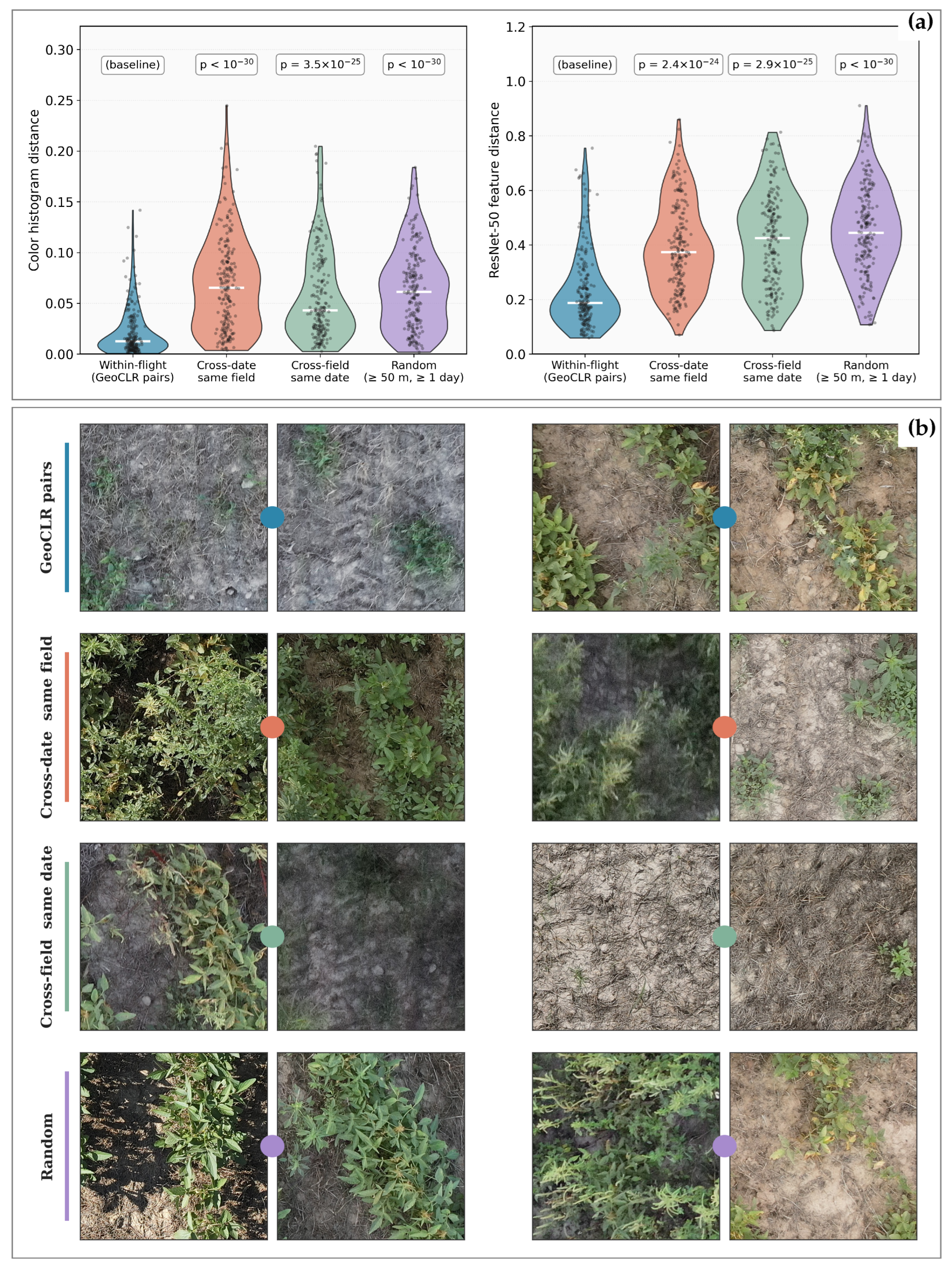
The SSL framework proposed in this study is based on the hypothesis that spatial overlap between adjacent UAS images within a flight provides a stronger positive-pair signal than synthetic augmentations alone, because overlapping images capture the same physical ground region under slightly different viewing angles, illumination conditions, and timing. To evaluate this empirically before constructing the SSL pipeline, a similarity analysis was conducted on 800 image pairs (200 pairs per condition) sampled from four conditions: (i) within-flight pairs, defined as image pairs from the same field and flight whose GPS positions were within 4 m and whose timestamps were within 180 s; (ii) cross-date same-field pairs, defined as image pairs from the same field collected on different dates; (iii) cross-field same-date pairs, defined as image pairs from different fields collected within seven days of each other; (iv) random pairs separated by at least 50 m and one day in time. For each image pair, two similarity distances were computed: a chi-squared distance between 32-bin RGB color histograms generated using the color analysis functions from PlantCV v4 [53], and a cosine distance between 2048-dimensional features extracted from the penultimate layer of an ImageNet-pretrained ResNet-50. The resulting similarity-distance distributions and representative image-pair examples across the evaluated pair-selection conditions are shown in Figure 3. Within-flight pairs showed approximately three-fold lower median color-histogram distance and two-fold lower median ResNet-50 feature distance compared to all other conditions, with all comparisons significant at $p<{10}^{-24}$ using one-sided Mann–Whitney U tests. These results support the use of within-flight overlap as the positive-pair signal for contrastive learning.

For each raw image in the unlabeled pretraining set, GPS coordinates, altitude, and timestamp were extracted from EXIF metadata recorded by the Zenmuse P1 camera. GPS coordinates were projected into local Universal Transverse Mercator (UTM, EPSG:32618) coordinates to calculate metric distance. Two images were considered candidate positive-pair sources if their GPS-derived ground positions were within 4 m and their timestamps were within 180 s. The 4 m spatial threshold was derived from the planned flight geometry. The ground footprint of each image was computed from the camera and flight parameters as

$$W_g={\displaystyle \frac{H·W_s}{f}},H_g={\displaystyle \frac{H·H_s}{f}},$$

where H is the flight altitude (12 m), $W_s$ and $H_s$ are the physical sensor width and height (35.9 mm and 24.0 mm for the Zenmuse P1 full-frame sensor), and f is the lens focal length (35 mm). This yields a ground footprint of approximately $12.3\times 8.2$ m per image. Given the $8192\times 5460$ pixel raw image resolution, this corresponds to ground sampling distances of

$${\displaystyle \frac{12.3\mathrm{m}}{8192\mathrm{pixel}}}\approx 0.150\mathrm{cm}/\mathrm{pixel}$$

along the image width and

$${\displaystyle \frac{8.2\mathrm{m}}{5460\mathrm{pixel}}}\approx 0.150\mathrm{cm}/\mathrm{pixel}$$

along the image height, consistent with the planned ground sampling distance. At the planned 80% frontal overlap, consecutive frames along the flight direction are spaced

$$d_{\mathrm{frame}}=(1-p_f)·W_g\approx 2.5\mathrm{m}$$

apart on the ground, where $p_f=0.80$ is the planned frontal overlap. The 4 m threshold therefore captures adjacent overlapping frames while allowing tolerance for GPS error and excluding most non-overlapping neighboring frames. The 180 s temporal threshold was selected to retain pairs from adjacent flight lines that overlap spatially because of the planned 70% side overlap but may be separated temporally by a full pass length. For each raw image, overlapping neighbors were identified by applying the 4 m and 180 s thresholds to all other images in the pretraining pool. Tile pairs were then constructed by sampling $640\times 640$ regions from the spatial overlap zone between the source image and one overlapping neighbor and extracting the corresponding tile from each image. Each tile was constrained to remain fully within its source-image boundary. This procedure was repeated $K=5$ times per source image, producing 7615 tiles from 1523 raw images in the SSL pretraining pool.

The extracted tiles covered a wide range of field conditions, including dense Palmer amaranth clusters, weeds overlapping with soybean canopy, treatment-boundary regions, and bare-soil patches. Positive pairs were intentionally similar but not identical, representing different views of the same physical region under slight variation in viewing angle, illumination, and framing. This variation encourages the encoder to learn features that are robust to nuisance factors instead of memorizing pixel-level appearance. During training, positive pairs were formed from overlapping image footprints satisfying the spatial and temporal thresholds, while negative pairs were formed implicitly within each batch from non-overlapping tiles. The 1523 unlabeled raw images used for SSL pretraining were collected from two RCBD field locations on a single flight date. Restricting SSL pretraining to a single date helped keep all positive pairs within the empirically validated within-flight condition. In contrast, the labeled object detection dataset spans multiple dates and growth stages, allowing evaluation of whether representations learned from a single-date SSL dataset transfer to downstream detection under varying field conditions. The raw images used for object detection annotation were not included in the SSL pretraining pool so that SSL pretraining and downstream detection evaluation remained fully separated. No image used during SSL pretraining later appeared as labeled training or validation data for the detection task.

The complete SSL framework proposed in this study is referred to as GeoCLR (Geographic Contrastive Learning of Representations). GeoCLR follows the encoder–projection-head architecture and NT-Xent contrastive loss used in SimCLR [46], but differs in how positive pairs are constructed. A shared encoder $f_{\theta }$ based on ResNet-50 was initialized from ImageNet-pretrained weights with the final classification layer removed. The encoder generated a 2048-dimensional feature representation for each image. A two-layer multilayer perceptron projection head $g_{\varphi }$ with one hidden layer of width 2048 and ReLU activation projected the encoder features into a 128-dimensional contrastive embedding space. To improve robustness to variation between overlapping views, each image underwent mild photometric augmentation, including random brightness, contrast, saturation, hue jitter, and occasional Gaussian blur. The NT-Xent loss for a positive pair $(i,j)$ within a batch of N positive pairs (yielding $2N$ tiles in total) was defined as

$${\mathcal{L}}_{i,j}=-\log {\displaystyle \frac{\exp (\mathrm{sim}(z_i,z_j)/{\tau }_c)}{{\sum }_{k=1}^{2N}⊮[k\ne i]\exp (\mathrm{sim}(z_i,z_k)/{\tau }_c)}}$$

where $z_i=g_{\varphi }\left(f_{\theta }\left(x_i\right)\right)$ denotes the projected embedding of tile $x_i$, $\mathrm{sim}(·,·)$ denotes cosine similarity, ${\tau }_c$ is the temperature parameter, and $⊮[·]$ is the indicator function. This objective pulls embeddings from positive-pair tiles closer together while separating embeddings from unrelated tiles within the same batch, allowing the encoder to learn features that remain stable under changes in viewpoint and illumination while still distinguishing different field regions. The GeoCLR encoder was trained for 200 epochs using a batch size of 32 and an input tile size of $640\times 640$ pixels. The temperature parameter was set to ${\tau }_c=0.5$. Optimization used stochastic gradient descent with momentum 0.9, weight decay of $5\times {10}^{-4}$, and an initial learning rate of 0.06 with cosine annealing over the full training schedule. After training, the projection head was discarded and the encoder weights were frozen for downstream evaluation. To evaluate whether GeoCLR-learned representations could distinguish Palmer amaranth from soybean, the frozen encoder was used to extract 2048-dimensional features from the held-out 468-image classification dataset. The resulting embeddings were visualized using Principal Component Analysis (PCA) and t-distributed Stochastic Neighbor Embedding (t-SNE) to assess class separability in the learned feature space. The same frozen encoder was then used as the backbone initialization for the Faster R-CNN-GeoCLR detector. The GeoCLR encoder weights replaced the standard ImageNet-pretrained backbone weights, while the feature pyramid network, region proposal network, and detection heads were trained from scratch during downstream detection training. Faster R-CNN was selected as the downstream detector because it is commonly used as a transfer-learning benchmark in SSL literature for object detection evaluation. Faster R-CNN-GeoCLR training and evaluation followed the same protocol described in Section 2.5.

2.5. Training and Evaluation

All training and inference experiments were conducted on the Virginia Tech Advanced Research Computing (ARC) Tinkercliffs cluster using NVIDIA A100 GPUs. To evaluate model generalization and reduce split-dependent bias, five-fold cross-validation was implemented [54]. The 2064 annotated image tiles were partitioned into five non-overlapping folds at the level of the original raw aerial image so that tiles extracted from the same aerial image never appeared in both training and validation sets. Fold assignment was stratified to balance Palmer amaranth and soybean instance counts across folds. Standardized training and evaluation settings shared across all detection models, SSL label-fraction experiments, and YOLO variant-size experiments are summarized in

Table 1. Standardized training and evaluation hyperparameters applied across all detection models, SSL label-fraction experiments, and YOLO variant-size experiments.

Hyperparameter	Value
Input image size	$640\times 640$ pixels
Batch size	32
Maximum epochs	150
Early stopping metric	Validation mAP@0.5
Early stopping patience	50 epochs
Cross-validation strategy	5-fold cross-validation
Random seed	42
GPU	NVIDIA A100 (80 GB)
CPU cores per run	4
Precision	FP32

. Architecture-specific settings were retained at their standard published configurations where appropriate.

To evaluate label efficiency, Faster R-CNN-GeoCLR was trained using 10%, 25%, 50%, and 100% of the annotated object detection training data within each fold. A nested subsampling strategy was used in which smaller label fractions formed strict subsets of larger ones. Specifically, the 10% subset was contained within the 25% subset, which was contained within the 50% subset, and all were contained within the full training set. Training images were deterministically ordered using a fixed random seed (seed = 42), and the first 10%, 25%, 50%, and 100% of the ordered list were selected for the respective experiments. This design ensured that performance differences across label fractions reflected only the effect of training-data volume rather than variation in sampled images. Validation was always performed on the full validation fold.

Beyond standard detection metrics, three deployment-oriented operational metrics were computed to evaluate how Palmer amaranth weed detector predictions translate into practical site-specific spraying outcomes: the weed coverage rate (WCR), the herbicide saving rate (HSR), and the weed coverage rate area under the curve (WCR-AUC). These metrics are more directly connected to field deployment because a weed detector with high mAP may still miss weeds outside the spray region or spray unnecessary areas. Spray geometry was modeled after the Ecorobotix^® (Yverdon, Switzerland) ARA field sprayer [55] as an operational example, which reports ultra-localized spraying precision of up to 6 cm × 6 cm. Each predicted weed detection retained at confidence threshold $\tau$ was assumed to trigger a single spray cell centered at the detection bounding-box centroid. At the ground sampling distance of 0.15 cm/pixel used in this study, each spray cell corresponded to a $40\times 40$ pixel region in image space.

Let G denote the set of ground-truth Palmer amaranth instances in an image, let I denote the image domain, and let $D\left(\tau \right)$ denote the set of detections retained after applying confidence threshold $\tau$. For any predicted detection $d\in D\left(\tau \right)$, let $c_d\in {\mathbb{R}}^2$ denote its centroid in pixel coordinates and let $C_d\left(\tau \right)\subset I$ denote the corresponding $40\times 40$ pixel spray cell centered at $c_d$. Similarly, for any ground-truth Palmer amaranth instance $g\in G$, let $c_g$ denote its annotated centroid.

WCR at threshold $\tau$ was defined as

$$\mathrm{WCR}\left(\tau \right)={\displaystyle \frac{1}{\left|G\right|}}\sum _{g\in G}⊮\left[\underset{d\in D\left(\tau \right)}{\min }{\parallel c_g-c_d\parallel }_{\infty }\le r\right]$$

where ${\parallel ·\parallel }_{\infty }$ denotes the Chebyshev ($L_{\infty }$) distance, $r=20$ pixels corresponds to half the spray-cell side length, and $⊮[·]$ is the indicator function. A ground-truth Palmer amaranth was considered covered if its centroid fell within the spray region of at least one retained detection.

HSR at threshold $\tau$ was defined as the proportion of image area that remained unsprayed:

$$\mathrm{HSR}\left(\tau \right)=1-{\displaystyle \frac{\left|{\bigcup }_{d\in D\left(\tau \right)}{C}_d\left(\tau \right)\right|}{\left|I\right|}}$$

where $\left|I\right|$ denotes the total image area. The union of spray cells was implemented using raster operations so that overlapping spray regions from adjacent detections were merged and counted only once.

Both WCR and HSR depend on the confidence threshold $\tau$, which determines which detections are retained as spray triggers. Existing precision-spraying studies [50] have reported these metrics only at fixed operating points, leaving no threshold-independent summary of detector performance. To address this limitation, this study introduces WCR-AUC, defined as the normalized area under the WCR($\tau$) curve over $\tau \in [0.05,0.95]$.

$$\mathrm{WCR}\text{-}\mathrm{AUC}={\displaystyle \frac{1}{{\tau }_{\max }-{\tau }_{\min }}}{\int }_{{\tau }_{\min }}^{{\tau }_{\max }}\mathrm{WCR}\left(\tau \right)d\tau$$

where ${\tau }_{\min }=0.05$ and ${\tau }_{\max }=0.95$. The integral was approximated using the trapezoidal rule with threshold increments of 0.05. WCR and HSR were reported at $\tau =0.25$ as representative single-operating-point operational metrics.

2.6. Statistical Analysis

To evaluate whether performance differences among object detection models were statistically significant, non-parametric statistical tests were used because the analysis involved paired measurements across five cross-validation folds without assuming normality of the performance metrics [56,57]. The Friedman test was first used as the global repeated-measures comparison across all models. The average rank of the $k^{th}$ model $(k=1,\dots ,K)$ was defined as

$$R_k={\displaystyle \frac{1}{J}}{\displaystyle \sum _{j=1}^J}{r}_k^j,$$

where J is the number of datasets (here $J=5$ folds) and $r_k^j$ is the rank assigned to the $k^{th}$ model in the $j^{th}$ fold. The Friedman statistic was then calculated as

$${\chi }_F^2={\displaystyle \frac{12J}{K(K+1)}}\left({\displaystyle \sum _{k=1}^K}{R}_k^2-{\displaystyle \frac{K{(K+1)}^2}{4}}\right),$$

which follows a chi-square distribution with $K-1$ degrees of freedom under the null hypothesis.

Because the Friedman test can be conservative for small sample sizes, the Iman–Davenport correction was also applied:

$$F_{ID}={\displaystyle \frac{(J-1){\chi }_F^2}{J(K-1)-{\chi }_F^2}},$$

which follows an F-distribution with $(K-1)$ and $(K-1)(J-1)$ degrees of freedom.

When the global test rejected the null hypothesis at $\alpha =0.05$, post hoc pairwise comparisons were performed using the Nemenyi test [58], which compares the average ranks of all detector pairs while controlling for multiple comparisons. The Nemenyi test was selected because it is commonly used as the post hoc procedure following the Friedman test for comparing multiple models across datasets or cross-validation folds.

Deployment-characteristic metrics including parameter count, GFLOPs, inference latency, throughput, and GPU memory usage were reported as point estimates and were not subjected to statistical testing because they depend on architecture design and inference hardware rather than fold-level variation. All statistical analyses were implemented in Python using the scipy and statsmodels libraries.

2.7. Overall Workflow

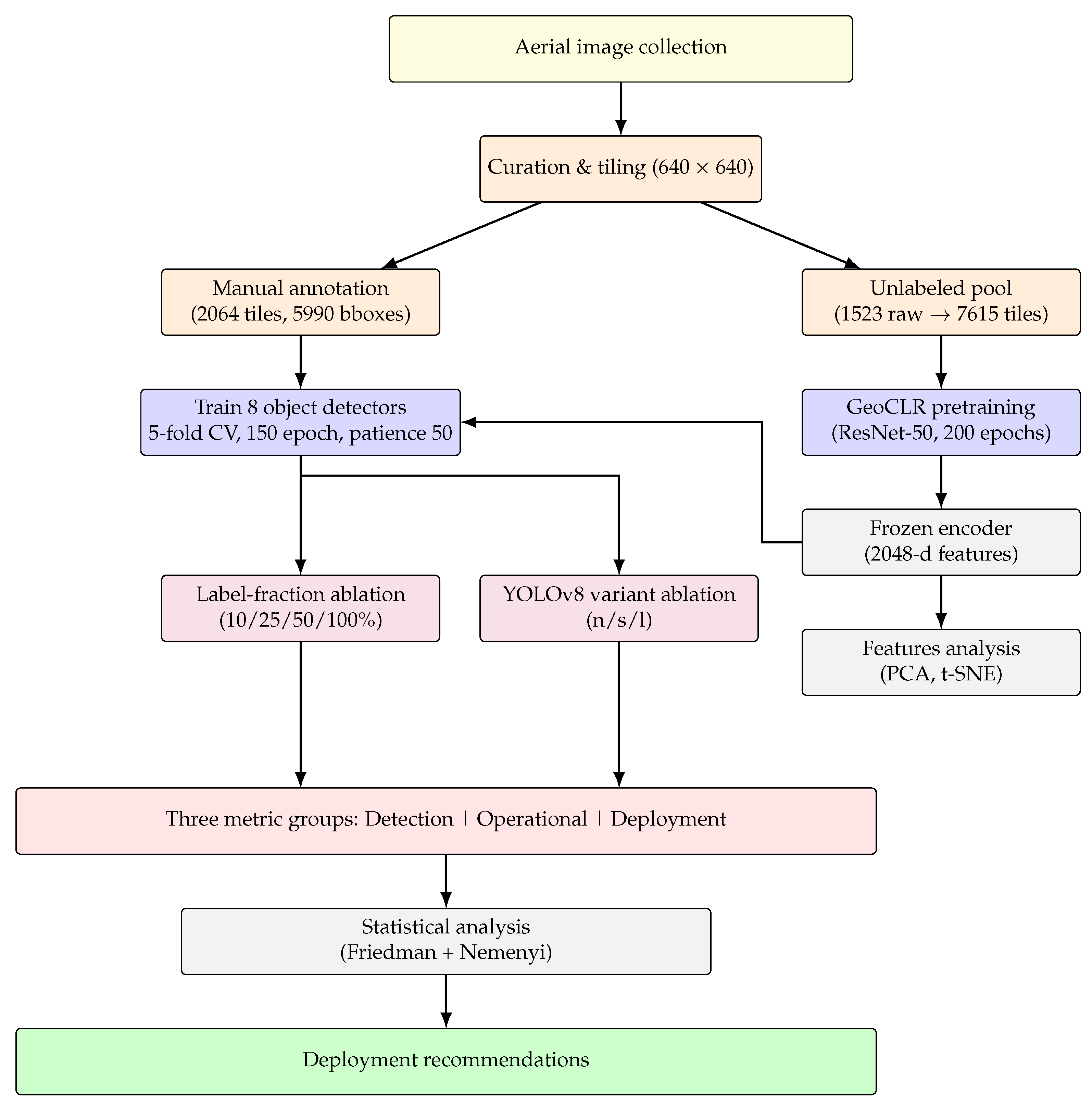
The complete experimental workflow used in this study is summarized in Figure 4. The pipeline consisted of two parallel branches originating from the same aerial image collection process. The first branch focused on supervised object detection benchmarking across multiple detector families, while the second branch focused on GeoCLR-based self-supervised pretraining using unlabeled aerial imagery.

The object detection branch included model benchmarking, YOLOv8 variant-size comparison, and label-fraction ablation experiments. The GeoCLR branch pretrained a ResNet-50 encoder using overlapping flight-image regions as positive pairs for contrastive learning. The pretrained encoder was then used for downstream transfer into Faster R-CNN-GeoCLR and for feature-space visualization.

Outputs from both branches were integrated into a unified evaluation stage consisting of detection, operational spraying, and deployment-oriented metrics, followed by statistical comparison and deployment-level interpretation.

3. Results

3.1. Detection Metrics Results

The eight object detection models were compared in terms of mAP at IoU thresholds of 0.5 and 0.5:0.95, as well as class-wise average precision for soybean and Palmer amaranth. All results are reported as mean ± standard deviation across the five cross-validation folds to indicate the stability of performance.

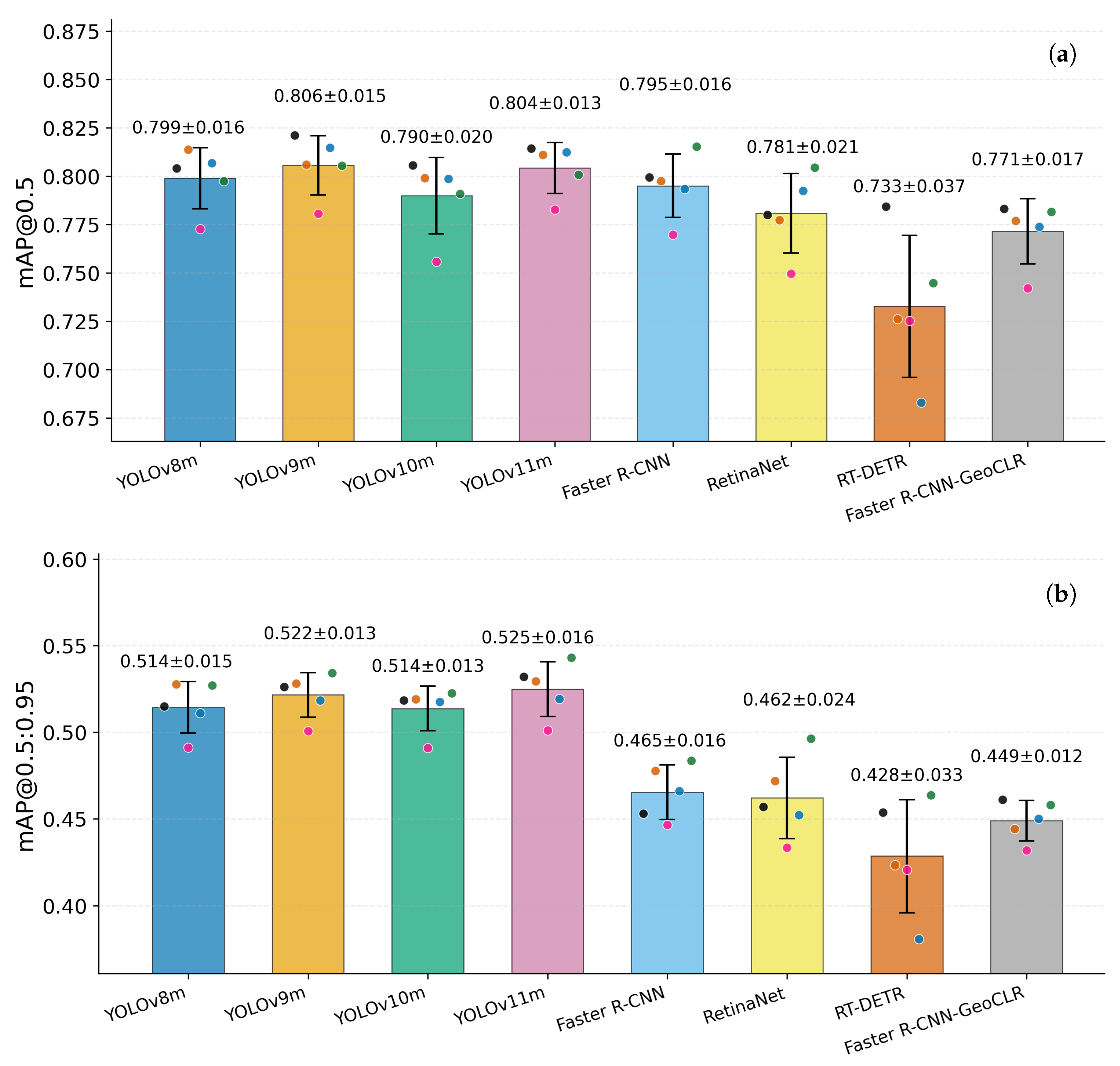
At IoU 0.5, the four YOLO models achieved similar mAP values in a narrow range of 0.790–0.806 (Figure 5a): YOLOv9m at 0.806 ± 0.015, YOLOv11m at 0.804 ± 0.013, YOLOv8m at 0.799 ± 0.016, and YOLOv10m at 0.790 ± 0.020. Faster R-CNN reached 0.795 ± 0.016, placing it within the YOLO performance range, while RetinaNet followed at 0.781 ± 0.021. Faster R-CNN-GeoCLR achieved 0.771 ± 0.017. RT-DETR recorded the lowest mAP@0.5 at 0.733 ± 0.037 and also showed the highest fold-to-fold variability. The relatively small standard deviations across folds indicate that detector performance remained stable across different train–test partitions of the dataset. At IoU 0.5, the overall gap between the strongest and weakest detectors was modest, spanning approximately 0.07 mAP.

The architectural differences became more apparent at the stricter IoU 0.5:0.95 threshold (Figure 5b). The four YOLO models maintained the highest performance, with mAP values in a narrow range of 0.514–0.525 (YOLOv11m at 0.525 ± 0.016, YOLOv9m at 0.522 ± 0.013, YOLOv8m at 0.514 ± 0.015, and YOLOv10m at 0.514 ± 0.013). In comparison, Faster R-CNN, RetinaNet, Faster R-CNN-GeoCLR, and RT-DETR dropped to 0.428–0.465, with RT-DETR recording the lowest value at 0.428 ± 0.033. The larger performance gap at the stricter IoU threshold suggests that the YOLO models produced more precise bounding-box localization, while the non-YOLO weed detectors were more strongly penalized as the overlap requirement increased.

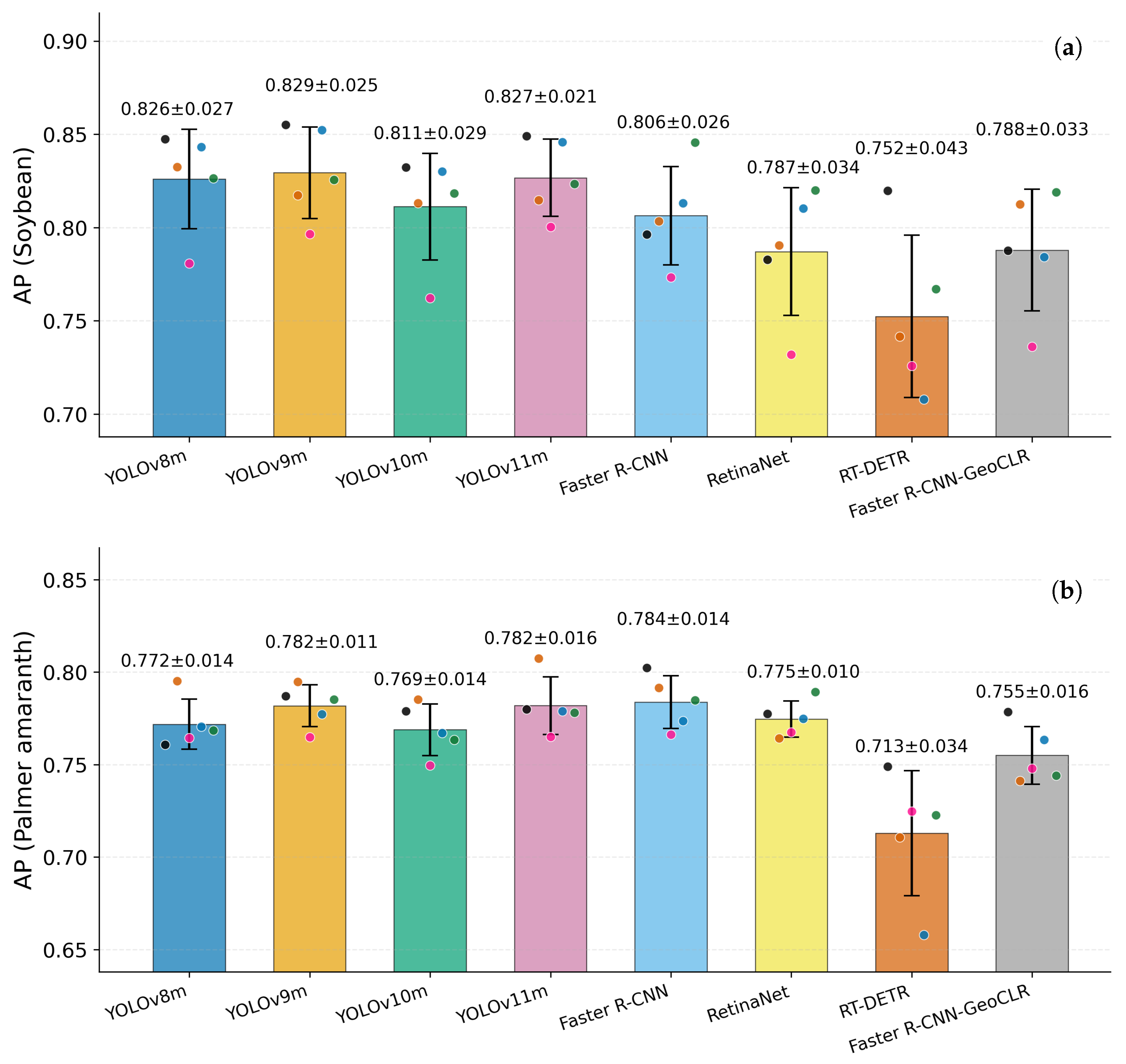
Class-specific average precision analysis showed that soybean was generally detected more accurately than Palmer amaranth across all weed detectors (Figure 6). For soybean, the YOLO variants performed nearly identically: YOLOv9m at 0.829 ± 0.025, YOLOv11m at 0.827 ± 0.021, YOLOv8m at 0.826 ± 0.027, and YOLOv10m at 0.811 ± 0.029. The non-YOLO weed detectors fell in a slightly lower band, with Faster R-CNN at 0.806 ± 0.026, Faster R-CNN-GeoCLR at 0.788 ± 0.033, and RetinaNet at 0.787 ± 0.034. RT-DETR recorded the lowest soybean AP at 0.752 ± 0.043. For Palmer amaranth, the eight detectors spanned a narrow range of 0.713–0.784. Faster R-CNN, YOLOv9m, and YOLOv11m sat at the top of this range (0.784, 0.782, and 0.782, respectively), with YOLOv8m (0.772 ± 0.014), RetinaNet (0.775 ± 0.010), and YOLOv10m (0.769 ± 0.014) only marginally behind. Faster R-CNN-GeoCLR achieved 0.755 ± 0.016 and RT-DETR recorded the lowest Palmer amaranth AP at 0.713 ± 0.034.

To assess whether the observed performance differences across weed detectors were statistically significant, mAP@0.5 was used as the primary metric for statistical testing, and the per-fold values were compared using the Friedman test. The Friedman test showed significant variation among the eight detectors (${\chi }^2\left(7\right)=26.73$, $p=3.7\times {10}^{-4}$), and the Iman–Davenport correction confirmed this result ($F=12.94$, $p<{10}^{-4}$). Average ranks across the five folds placed YOLOv9m first (mean rank 1.8), followed by YOLOv11m (2.2) and YOLOv8m (3.2), while RT-DETR ranked lowest (7.6) and Faster R-CNN-GeoCLR second-lowest (7.0). Post hoc pairwise comparisons using the Nemenyi test identified significant differences primarily between the strongest and weakest detectors. YOLOv9m and YOLOv11m both significantly outperformed RT-DETR ($p=0.0045$ and $p=0.0115$, respectively) and Faster R-CNN-GeoCLR ($p=0.0180$ and $p=0.0409$, respectively). No additional pairwise comparisons reached the significance threshold. The large middle group of detectors, including YOLOv8m, YOLOv10m, Faster R-CNN, and RetinaNet, could not be statistically separated from one another or from the top-ranked YOLO models at IoU 0.5. This result suggests that although the strongest YOLO variants showed measurable advantages over the weakest detectors, most architectures achieved relatively similar performance under the permissive IoU 0.5 criterion. The limited number of folds ($n=5$) also reduces the power of the pairwise comparisons to resolve smaller differences among closely clustered weed detectors.

3.2. Operational Metrics Results

Operational performance results were computed under the simulated precision-spraying protocol described in Section 2.5, in which each retained detection triggered a single $6\times 6$ cm spray cell modeled after the Ecorobotix^® ARA commercial sprayer [55]. Results are reported as mean ± standard deviation across the five cross-validation folds (

Table 2. Operational metrics for the eight Palmer amaranth weed detectors evaluated under the simulated precision-spraying protocol using a $6\times 6$ cm spray cell. WCR and HSR are reported at $\tau =0.25$, while WCR-AUC summarizes weed coverage across $\tau \in [0.05,0.95]$. Values are reported as mean ± standard deviation across five cross-validation folds.

Detector	WCR @ $\mathit{\tau }=0.25$	HSR @ $\mathit{\tau }=0.25$	WCR-AUC
Faster R-CNN	$0.705\pm 0.018$	$0.979\pm 0.003$	$0.664\pm 0.018$
Faster R-CNN-GeoCLR	$0.685\pm 0.037$	$0.980\pm 0.004$	$0.645\pm 0.034$
RT-DETR	$0.790\pm 0.025$	$0.968\pm 0.007$	$0.609\pm 0.046$
RetinaNet	$0.697\pm 0.013$	$0.984\pm 0.001$	$0.535\pm 0.031$
YOLOv9m	$0.632\pm 0.015$	$0.991\pm 0.001$	$0.501\pm 0.009$
YOLOv11m	$0.636\pm 0.008$	$0.991\pm 0.000$	$0.496\pm 0.015$
YOLOv10m	$0.605\pm 0.012$	$0.992\pm 0.000$	$0.488\pm 0.019$
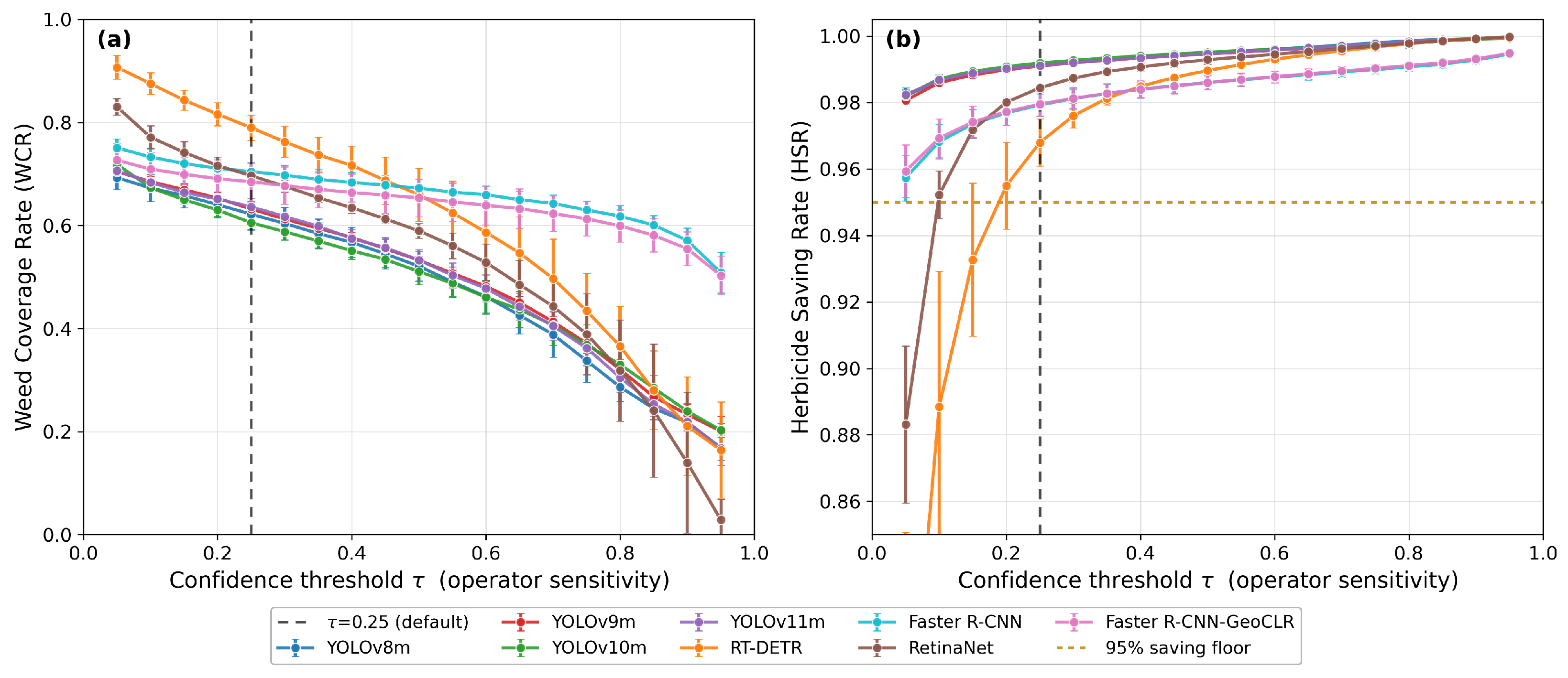
YOLOv8m	$0.622\pm 0.031$	$0.991\pm 0.001$	$0.483\pm 0.027$

). HSR showed limited variation across most detectors. At $\tau =0.25$, HSR ranged from 0.968 to 0.992, indicating that all detectors triggered spray coverage over only a small fraction of the total image area. The per-threshold analysis shown in Figure 7 indicated that HSR exceeded 0.97 by $\tau =0.15$ for six of the eight detectors; RT-DETR, which produced the highest volume of low-confidence detections, reached that level by $\tau =0.25$. The largest HSR reductions occurred at low confidence thresholds ($\tau \le 0.10$), where RT-DETR and RetinaNet produced larger numbers of low-confidence detections that activated additional spray cells.

Compared with HSR, WCR and WCR-AUC provided stronger separation among detectors. Faster R-CNN achieved the highest WCR-AUC at $0.664\pm 0.018$, followed by Faster R-CNN-GeoCLR at $0.645\pm 0.034$ and RT-DETR at $0.609\pm 0.046$. RetinaNet followed at $0.535\pm 0.031$, while the four YOLO models produced the lowest WCR-AUC values, ranging from 0.483 to 0.501.

The statistical significance of the WCR-AUC ranking was evaluated using the same Friedman + Nemenyi framework described in Section 2.6. The Friedman test rejected the null hypothesis of equal detector performance (${\chi }^2\left(7\right)=28.73$, $p=1.6\times {10}^{-4}$), and the Iman–Davenport correction confirmed this result ($F=18.34$, $p<{10}^{-5}$). Average WCR-AUC ranks placed Faster R-CNN highest (1.2), followed by Faster R-CNN-GeoCLR (2.0) and RT-DETR (3.0), while the YOLO models occupied the four lowest ranks (6.0–7.0). Post hoc Nemenyi comparisons showed that Faster R-CNN significantly outperformed all four YOLO models (p = 0.005–0.041), and Faster R-CNN-GeoCLR significantly outperformed YOLOv10m (p = 0.027). No additional pairwise differences reached statistical significance.

The threshold-dependent behavior of the detectors is shown in Figure 7a. RT-DETR achieved the highest WCR at the default operating point ($0.790\pm 0.025$ at $\tau =0.25$), exceeding Faster R-CNN by approximately 0.085. However, RT-DETR coverage decreased more rapidly as the confidence threshold increased, causing its overall WCR-AUC to fall below both Faster R-CNN variants. In contrast, Faster R-CNN maintained more stable weed coverage across the full threshold range.

3.3. Deployment Metrics Results

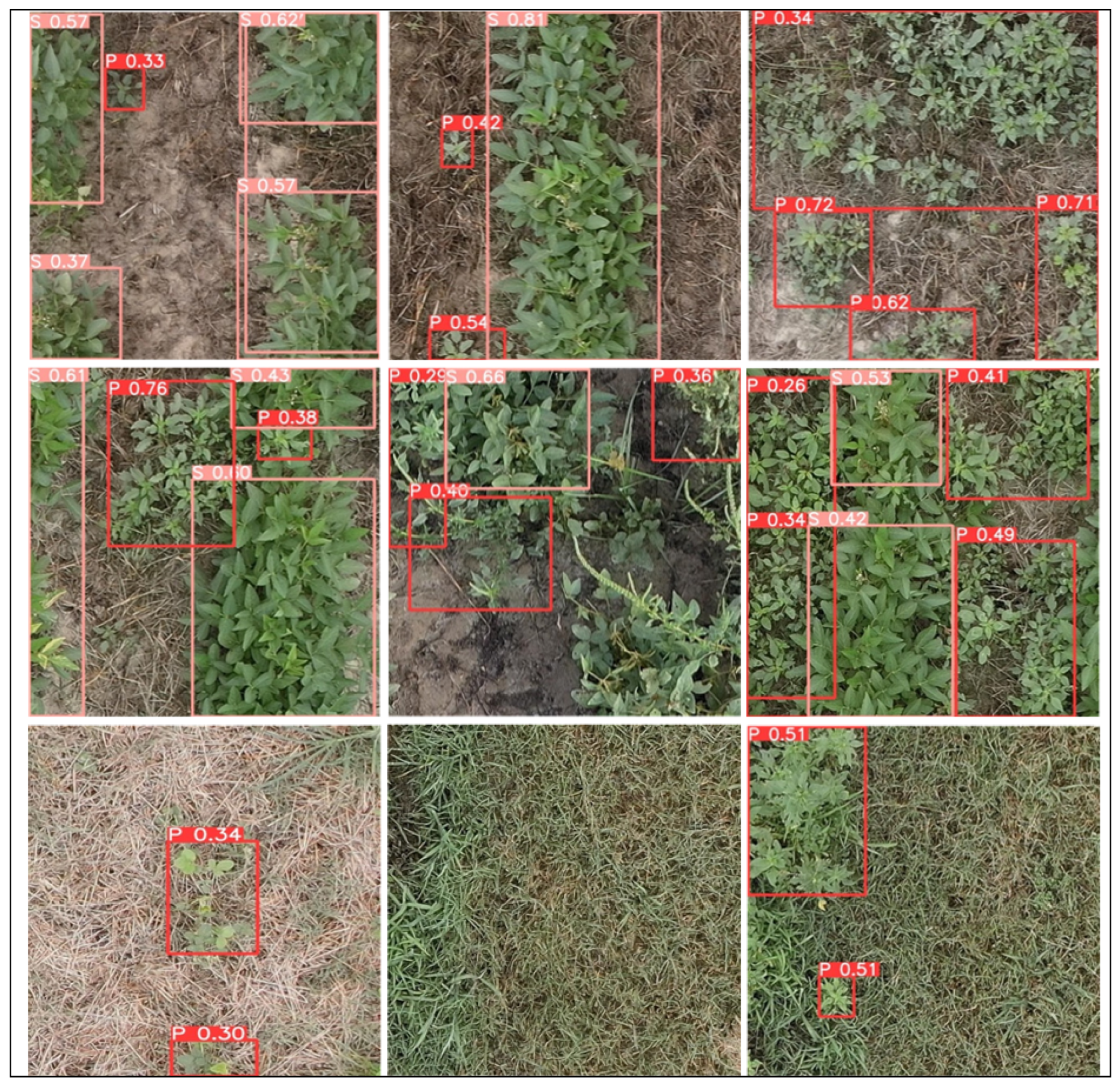
Deployment characteristics were benchmarked for all eight detectors on a single NVIDIA A100 GPU using $640\times 640$ input resolution and FP32 precision. Batch sizes of 1, 4, 8, 16, and 32 were evaluated. For each configuration, latency was measured over 200 timed iterations following 50 warm-up iterations. Five deployment metrics were recorded: parameter count, GFLOPs, inference latency, throughput in frames per second (FPS), and peak GPU memory usage. To complement the quantitative deployment metrics, representative prediction examples generated by YOLOv8m on held-out aerial field images that were not part of the annotated object detection dataset are shown in Figure 8. These examples span a range of Palmer amaranth densities, canopy overlap conditions, and field backgrounds observed across the test imagery and serve as a visual reference rather than for quantitative evaluation.

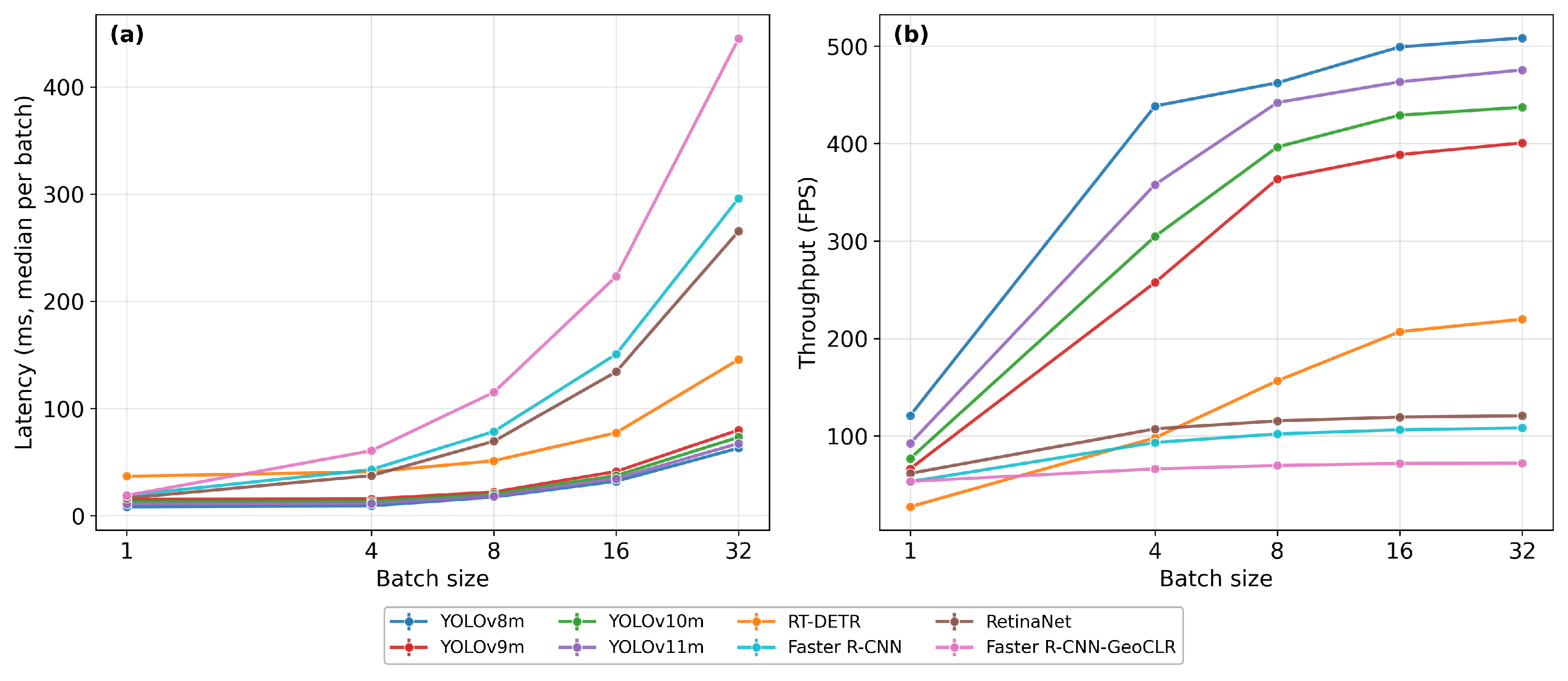
Headline deployment metrics at batch size 1, representing the regime most relevant for real-time field deployment, are summarized in

Table 3. Deployment metrics for the eight detectors measured on a single NVIDIA A100 GPU at $640\times 640$ input resolution and FP32 precision. Latency, FPS, and GPU memory usage are reported at batch size 1. Latency values represent the median over 200 timed iterations following 50 warm-up iterations.

Detector	Params (M)	GFLOPs	Latency (ms)	FPS	GPU Mem (GB)
YOLOv8m	25.9	39.5	8.3	120.9	0.31
YOLOv9m	20.2	38.8	15.1	66.2	0.30
YOLOv10m	16.5	32.0	13.0	76.7	0.30
YOLOv11m	20.1	34.1	10.8	92.3	0.34
RT-DETR	32.8	54.0	36.7	27.2	0.50
Faster R-CNN	41.1	89.0	18.9	53.0	0.72
RetinaNet	36.1	79.8	16.3	61.5	1.08
Faster R-CNN-GeoCLR	43.3	280.4	18.8	53.2	1.03

, while batch-size scaling of latency and throughput is presented in Figure 9.

The eight detectors spanned a broad range of model sizes, from 16.5 M parameters for YOLOv10m to 43.3 M for Faster R-CNN-GeoCLR. At batch size 1, the YOLO models achieved the lowest inference latency. YOLOv8m was fastest at 8.3 ms per frame (120.9 FPS), followed by YOLOv11m at 10.8 ms (92.3 FPS), YOLOv10m at 13.0 ms (76.7 FPS), and YOLOv9m at 15.1 ms (66.2 FPS). RetinaNet and the two Faster R-CNN variants formed a middle group at 16.3–18.9 ms (53–62 FPS). RT-DETR showed the highest single-frame latency at 36.7 ms (27.2 FPS).

The batch-size sweep showed clear differences in scaling behavior across architectures (Figure 9). The YOLO models scaled most efficiently, with throughput increasing strongly as batch size increased. YOLOv8m reached approximately 508 FPS at batch size 32. RT-DETR also scaled well under batching, increasing from 27 FPS at batch size 1 to 220 FPS at batch size 32, suggesting that a larger portion of its runtime comes from fixed computational overhead that becomes amortized under larger batches. In contrast, Faster R-CNN, Faster R-CNN-GeoCLR, and RetinaNet scaled more slowly, reaching approximately 72–121 FPS at batch size 32. These differences are important for deployment because single-frame systems depend mainly on low inference latency, while buffered systems benefit more from high batched throughput.

GPU memory usage generally followed model size and architecture complexity. At batch size 1, the YOLO models required only 0.30–0.34 GB of GPU memory, RT-DETR required 0.50 GB, and the two-stage detectors required 0.72–1.08 GB. The gap widened further under batching. At batch size 32, the YOLO models and RT-DETR remained between 2.46 and 3.63 GB, whereas Faster R-CNN reached 6.70 GB and Faster R-CNN-GeoCLR reached 10.57 GB.

3.4. Self-Supervised Feature Analysis

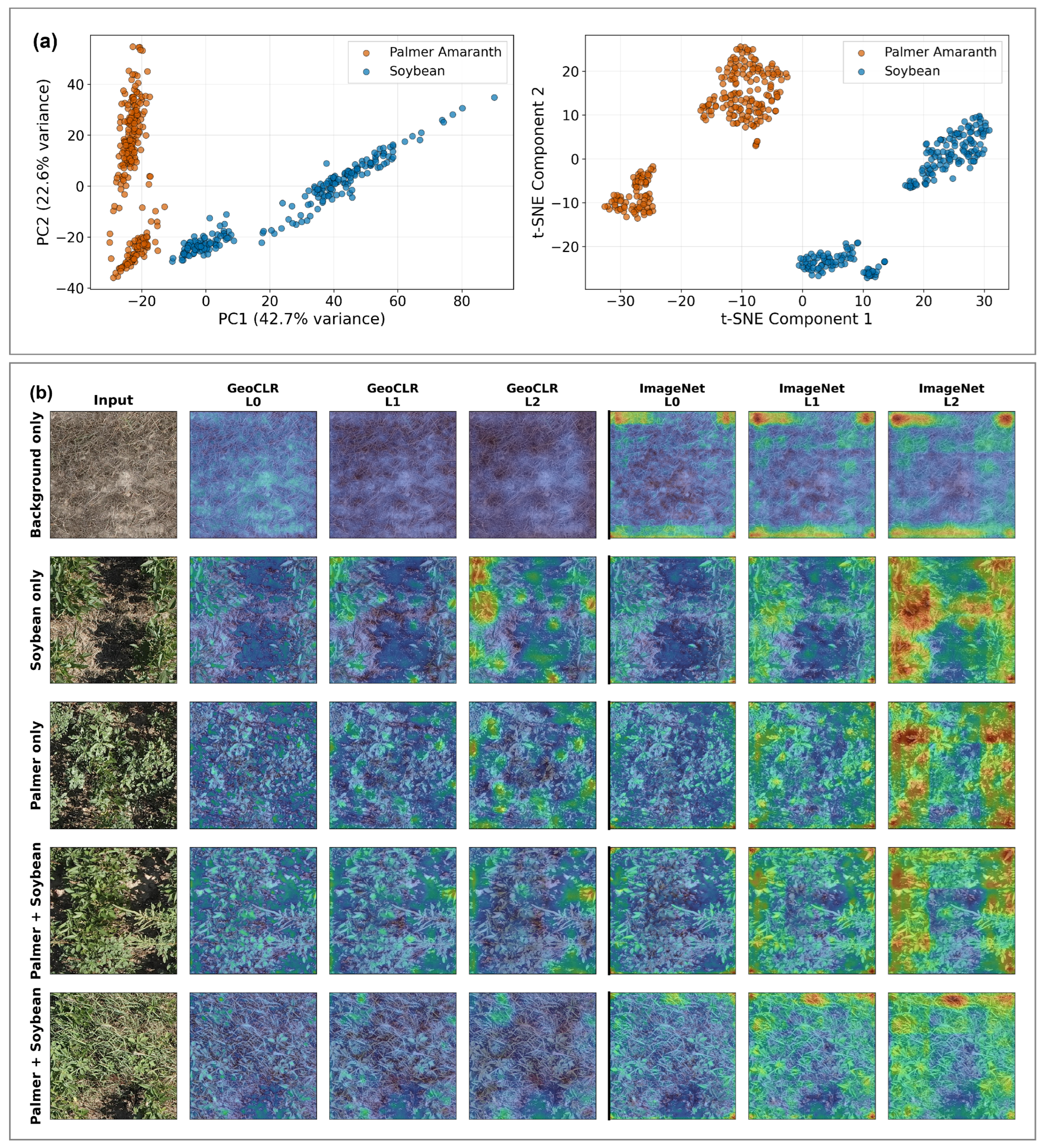
To better understand what the GeoCLR self-supervised pretraining contributed beyond downstream detection accuracy, the learned ResNet-50 backbone was analyzed in two complementary ways: (i) separability of the learned feature embeddings for Palmer amaranth and soybean, and (ii) spatial activation structure across network depth. In both analyses, the GeoCLR-pretrained backbone was compared against an ImageNet-pretrained backbone of identical architecture, with all feature extraction and processing steps kept identical so that any observed differences were attributable to the pretraining strategy alone. Both pretraining schemes produced class-separable features, which is expected given the visual differences between Palmer amaranth and soybean. However, the GeoCLR backbone separated the two classes substantially more cleanly and compactly than the ImageNet-pretrained backbone. The frozen GeoCLR backbone produced clear separation between Palmer amaranth and soybean in the feature space (Figure 10a). In the PCA projection, the two classes separated primarily along PC1, which explained 42.7% of the variance, while PC2 explained an additional 22.6%, resulting in 65.3% cumulative variance captured by the first two principal components. In contrast, the first two principal components of the ImageNet-pretrained backbone captured only 20.3% of the total variance, indicating that the GeoCLR features concentrated the class-relevant structure into a substantially lower-dimensional subspace.

The t-SNE projection showed a similar trend, with Palmer amaranth and soybean forming compact and well-separated clusters under GeoCLR pretraining. This improvement was also reflected quantitatively by the silhouette coefficient computed on the full 2048-dimensional feature space, which increased from 0.113 for the ImageNet-pretrained backbone to 0.335 for the GeoCLR backbone, representing approximately a threefold improvement in class separation quality. Together, the embedding projections and silhouette analysis showed stronger class separation under GeoCLR pretraining than under ImageNet pretraining.

To characterize how the two backbones responded spatially across network depth, activation maps were extracted from three successive feature levels (L0, L1, and L2) for representative aerial tiles spanning background-only regions, soybean-dominant regions, Palmer-dominant regions, and mixed Palmer–soybean scenes (Figure 10b). Activation maps from the GeoCLR-pretrained and ImageNet-pretrained backbones were visualized using the same normalization scale at each level so that differences in intensity reflected differences in feature response rather than independent per-image rescaling. The clearest difference between the two backbones appeared in the background-only tile. Across all three feature levels, the GeoCLR backbone produced relatively weak and spatially uniform responses over bare soil and crop-residue regions, and this suppression became stronger at deeper levels. By L2, the background region was largely quiescent with only limited localized activation remaining. In contrast, the ImageNet-pretrained backbone produced broader responses across the same background tile, including strong activations near image borders and corners that became increasingly pronounced at deeper levels. A similar trend was observed across tiles containing vegetation. In the soybean-only, Palmer-only, and mixed Palmer–soybean scenes, the GeoCLR backbone produced more spatially coherent and selective responses that increasingly concentrated around vegetation structure with depth. The ImageNet-pretrained backbone produced broader responses extending further into background texture and edge regions, particularly at the deeper L2 level.

3.5. Ablation Studies

Two ablation studies were conducted to support key methodological decisions used throughout the main benchmark. The first evaluated whether increasing detector capacity materially changed detection accuracy within the YOLOv8 family, addressing the choice of the medium-capacity variant used in the main experiments. The second evaluated the label efficiency of the Faster R-CNN-GeoCLR by quantifying how detection performance changes as the amount of annotated training data is reduced.

3.5.1. Effect of Model Scale

The main benchmark used the medium-capacity variant for each YOLO family. To determine whether this choice influenced the comparative results, additional experiments were conducted using the nano, small, and large variants of YOLOv8 under the identical 5-fold cross-validation protocol, training schedule, and data splits used in the primary benchmark (

Table 4. Effect of YOLOv8 model scale on detection performance. All variants were trained using the identical 5-fold cross-validation protocol, training schedule, and data splits. Values are reported as mean ± standard deviation across the five folds.

YOLOv8 Variant	mAP@0.5	mAP@0.5:0.95
Nano (n)	$0.797\pm 0.006$	$0.511\pm 0.007$
Small (s)	$0.785\pm 0.020$	$0.503\pm 0.012$
Large (l)	$0.800\pm 0.014$	$0.517\pm 0.010$

).

Detector scale produced only modest differences in accuracy. Mean mAP@0.5 ranged from 0.785 to 0.800 across the three additional variants, corresponding to a spread of approximately 1.5 percentage points. The relationship between model size and performance was also non-monotonic: the nano variant achieved performance comparable to the large variant, while the small variant produced a similar mean accuracy of 0.785. The medium-capacity model used in the primary benchmark fell within this same narrow performance range. Similar trends were observed for mAP@0.5:0.95.

These results suggest that, for this two-class aerial weed-detection task, increasing detector capacity beyond the medium regime provides limited accuracy benefit relative to the additional computational cost. The medium-capacity variants therefore provided a reasonable tradeoff between detection performance and deployment efficiency, while also enabling a consistent comparison across detector families.

3.5.2. Label Efficiency of GeoCLR

Because GeoCLR pretraining operates entirely on unlabeled aerial imagery, only the detector fine-tuning stage requires manually annotated bounding-box labels. To quantify how detection performance scales with annotation availability, the Faster R-CNN-GeoCLR was fine-tuned using 10%, 25%, 50%, and 100% of the available manually annotated training datasets, as described in Section 2.5 (

Table 5. Label efficiency of the Faster R-CNN-GeoCLR. The detector was fine-tuned using increasing fractions of the available training annotations. Values are reported as mean ± standard deviation across the five folds.

Label Fraction	mAP@0.5	mAP@0.5:0.95	% of Full-Data mAP@0.5
10%	$0.622\pm 0.008$	$0.327\pm 0.012$	80.6%
25%	$0.687\pm 0.015$	$0.381\pm 0.013$	89.0%
50%	$0.730\pm 0.017$	$0.418\pm 0.014$	94.6%
100%	$0.772\pm 0.017$	$0.449\pm 0.012$	100.0%

).

Detection accuracy increased rapidly at low annotation fractions and then gradually approached saturation as additional bounding-box annotations were introduced. Using only 10% of the annotated training datasets, the detector achieved an mAP@0.5 of 0.622, corresponding to 80.6% of the full-data performance. At 50% of the annotated training set, performance increased to 0.730 mAP@0.5, recovering 94.6% of the full-data result. Similar behavior was observed for mAP@0.5:0.95, which increased from 0.327 at 10% labels to 0.418 at 50%.

The performance gains per additional annotation fraction progressively decreased as more bounding-box labels were added. Increasing the label fraction from 10% to 25% improved mAP@0.5 by 0.065, whereas increasing the label fraction from 50% to 100% improved performance by only 0.042. This indicates that much of the discriminative representation learned through GeoCLR pretraining can already be transferred using a relatively small subset of manually annotated bounding boxes.

4. Discussion

This study evaluated weed detection models from a practical precision-agriculture perspective. The goal was not only to identify which detector produced the highest accuracy, but also to understand which models may be useful for site-specific spraying. For agricultural users, this distinction is important because a model with strong detection accuracy is not automatically the best model for field deployment. A useful spraying model should detect weeds reliably, maintain good weed coverage across confidence thresholds, and run fast enough for the intended hardware platform.

The results showed that detector rankings changed depending on the evaluation criterion. The YOLO models achieved the strongest detection accuracy and the lowest computational cost, while the Faster R-CNN models showed stronger threshold-independent weed coverage. This means that model selection should depend on the final use case. A real-time UAS or edge-based spraying workflow may favor a faster detector, whereas an offline mapping or decision-support workflow may tolerate a slower model if weed coverage is the main objective. GeoCLR also addressed a different but related problem: reducing dependence on large manually labeled datasets by learning useful representations from unlabeled overlapping UAS images.

4.1. Suitability of YOLO Architectures for Aerial Weed Detection

The four YOLO variants achieved the highest detection accuracy, and their advantage became more apparent at the stricter mAP@0.5:0.95 threshold. This suggests that the YOLO models did not only identify the correct plant class, but also localized plant regions more accurately than the two-stage, transformer-based, and non-YOLO single-stage detectors evaluated in this study. This result is consistent with prior weed-detection studies showing that YOLO-based models are effective for crop-weed detection in field images, including Palmer amaranth detection in soybean and cotton systems [36,40,41].

At the same time, previous weed-detection studies were often limited to fewer model generations, smaller datasets, ground-level imagery, or more controlled field conditions [36,40,59,60]. The present study extends this earlier work by comparing recent YOLO generations with two-stage, transformer-based, and non-YOLO single-stage detectors using high-resolution aerial imagery collected across multiple plant growth stages. This broader comparison is important because recent work has also shown that newer YOLO versions do not always outperform older versions under all weed-detection conditions [41]. Therefore, agricultural users should select models based on field performance, deployment needs, and operating conditions rather than model release order alone.

One likely reason the YOLO family performed well is that the image structure matched the strengths of single-stage detection. The aerial tiles contained many small and broadly similar-scale plant instances against relatively uniform field backgrounds. The single-stage YOLO design with multi-scale feature aggregation appears well matched to this type of dense small-object detection. In comparison, RT-DETR relies on attention over a limited set of object queries, which may be less suitable when many small plant instances occur within the same aerial tile. Similarly, the additional proposal stage used by Faster R-CNN did not improve localization accuracy under these relatively homogeneous field conditions. These findings support the broader observation that YOLO models can be strong candidates for field deployment when speed and localization quality are both important [61,62].

Soybean was generally easier to detect than Palmer amaranth across nearly all detectors. As described in Section 2.2, soybean foliage had a higher excess-green index than Palmer amaranth and therefore showed stronger contrast against the soil background. Soybean plants were also larger on average, with a median bounding-box area approximately 1.68 times larger than Palmer amaranth. Larger and visually distinct objects are easier to localize in aerial imagery, while Palmer amaranth showed greater variation in morphology, overlap, and canopy density across growth stages. These visual differences likely explain why soybean detection accuracy was consistently higher than Palmer amaranth detection accuracy.

4.2. Detection Accuracy and Operational Spraying Behavior Are Not Equivalent

A major finding of this study is that detection accuracy and spraying usefulness are related but not identical. Standard object detection metrics such as mAP reward correct class prediction, confidence, and bounding-box overlap. These metrics are important, but they do not directly show whether the predicted spray region would cover the weed in a practical spraying workflow. For this reason, deployment-oriented metrics such as WCR, HSR, and WCR-AUC provide additional information that mAP alone cannot provide [50].

The difference between mAP and operational spraying behavior was especially clear when comparing YOLO and Faster R-CNN. The YOLO models achieved the highest mAP values, but the Faster R-CNN models achieved stronger threshold-independent weed coverage across confidence levels. This means that a detector can be accurate by standard computer-vision criteria but still behave differently when translated into a spraying decision. For example, a detector may produce high-confidence boxes that improve mAP, but if detections become unstable across thresholds, the effective spray coverage may decline. RT-DETR showed this issue clearly. It achieved high weed coverage at lower confidence thresholds, but coverage declined rapidly as the confidence threshold increased. This led to lower WCR-AUC despite competitive low-threshold behavior. In contrast, Faster R-CNN maintained more stable weed coverage across thresholds, even though its mAP was lower than the best YOLO models. The HSR metric showed less separation among detectors because the simulated spray-cell area occupied only a small fraction of the image across models. Under these imaging and simulation conditions, operational performance was driven more by weed coverage than by sprayed area.

These findings have practical implications for precision spraying. If the goal is to build a real-time spraying system, model evaluation should include both detection accuracy and spraying behavior. Reporting only mAP may lead to selecting a model that performs well on benchmark metrics but is not optimal for actual spray coverage. Threshold-independent metrics such as WCR-AUC are therefore useful because they show how robustly a detector covers weeds across the confidence range used in deployment.

4.3. Detector Selection for Field Deployment

No single architecture dominated across all evaluation axes. YOLOv8m provided the most balanced deployment profile by combining strong detection accuracy, low latency, high throughput, and relatively low GPU memory usage. This makes YOLOv8m a practical candidate for real-time or near-real-time aerial spraying workflows. In contrast, Faster R-CNN provided stronger weed coverage across thresholds but required substantially more computational resources. Therefore, Faster R-CNN may be more useful for offline weed mapping, generating field maps that guide where herbicide should be applied, or decision-support systems where speed is less restrictive.

The deployment results also show why the intended operating mode should guide model choice. For on-board UAS inference or edge-computing systems, single-image latency and memory cost are critical because the model must process images quickly during flight or immediately after acquisition. Under this use case, the YOLO family is more practical than heavier two-stage or transformer-based models. For buffered post-flight processing, however, batching can reduce the penalty of slower architectures. RT-DETR, for example, had slow single-frame inference but scaled more efficiently under batching. This suggests that transformer-based models may be more suitable for offline processing than for direct real-time spraying.

These findings extend previous UAS and precision-agriculture studies by evaluating accuracy, spraying behavior, and computational cost together. Prior studies have commonly emphasized mAP or F1-score or latency, while deployment-related metrics such as throughput, memory use, and spraying coverage are less often reported together [36,40,41,50]. The current results show that these evaluation axes can lead to different model rankings. For practical agricultural deployment, this means that detector selection should be based on the full workflow rather than a single accuracy metric.

4.4. Significance of GeoCLR

GeoCLR was developed to address the labeling challenge in UAS-based weed detection. Manual annotation of weed and crop bounding boxes is time-consuming, especially when datasets must cover different fields, seasons, growth stages, and image acquisition conditions. GeoCLR uses spatial overlap between adjacent UAS images to form positive pairs for self-supervised pretraining. This is different from standard augmentation-based contrastive learning, where positive pairs are usually created only from transformed versions of the same image. The approach builds on the idea that naturally occurring spatial or temporal relationships can provide useful supervision for representation learning [46,48,49].

The feature analysis showed that GeoCLR produced stronger class separation than standard ImageNet pretraining. On the held-out classification dataset, the GeoCLR backbone separated Palmer amaranth and soybean more clearly than an ImageNet-pretrained backbone of the same architecture, with a silhouette coefficient of 0.335 compared with 0.113. The GeoCLR features were also more compact, with most class-related variation concentrated into a lower-dimensional subspace. The activation-map analysis showed a similar pattern: deeper GeoCLR features responded more selectively to vegetation structure while suppressing more homogeneous background regions.

The main benefit of GeoCLR was not a large increase in fully supervised detection mAP. Faster R-CNN-GeoCLR remained close to the standard ImageNet-pretrained Faster R-CNN, with only a small gap in mAP@0.5. The stronger practical contribution was label efficiency. Because GeoCLR uses unlabeled aerial imagery during pretraining, it recovered 80.6% of full-data accuracy using only 10% of the annotations and 94.6% using half of the annotations. This pattern is consistent with prior agricultural self-supervised learning studies showing that SSL is often most useful when labeled data are limited [63,64,65].

For weed scientists and agricultural engineers, this result is useful because UAS imagery is often easier to collect than to annotate. Large collections of routine aerial images could be used for pretraining, and only a smaller subset may need manual labeling for downstream detection. This could reduce the cost and time required to build new weed-detection models for additional fields, seasons, or crop systems. Recent weed dataset studies have also highlighted that public weed datasets are limited by variation, distribution shift, and cross-season generalization challenges [66]. Under these conditions, methods that use unlabeled imagery more effectively may help improve model development when large labeled datasets are unavailable.

4.5. Limitations and Future Work

Several limitations should be considered when interpreting these results. Most of the dataset was collected under experimental field conditions with a single soybean cultivar in one U.S. region and under controlled weed-density treatments. Commercial production fields can be more variable, with mixed weed species, irregular canopy structure, different soil backgrounds, and changing illumination. Therefore, the detectors evaluated here should be interpreted as benchmarked under controlled aerial acquisition conditions rather than fully validated for commercial deployment across all soybean systems.

Future studies should test these models across additional locations, soybean cultivars, weed communities, growth stages, flight conditions, and management systems. Field management practices such as tillage, strip-till, and no-till systems may change soil background, residue cover, canopy structure, and weed visibility. Weather and imaging conditions, including cloud cover, shadows, sun angle, and illumination changes, may also affect detection accuracy and spraying behavior. Evaluating these factors will be important before deployment in broader commercial settings.

The analysis also did not explicitly separate performance by growth stage, although the dataset included multiple soybean and Palmer amaranth growth stages. This is important because both species change substantially during canopy development, especially when plants overlap or weed density increases. The YOLOv8 variant-size ablation suggested that increasing model capacity beyond the medium-scale model produced only limited performance improvement. This indicates that dataset diversity may currently be a larger limitation than model size for this task.

GeoCLR pretraining was restricted to a single flight date so that all positive pairs satisfied the empirically validated within-flight overlap condition. Future work should evaluate whether the same framework generalizes across seasons, locations, crop systems, and acquisition conditions. Additional comparisons with other self-supervised approaches would also help determine how much of the observed improvement is specific to GeoCLR.

Finally, this study evaluated detection-derived operational metrics using simulated spraying behavior. Additional field validation is needed to determine how these weed maps translate into herbicide savings, economic return, weed control efficacy, and reducing crop yield loss under real spraying conditions.

5. Conclusions

This study compared eight object detection models for Palmer amaranth and soybean detection in high-resolution aerial imagery. The models were evaluated using detection accuracy, spraying-oriented operational behavior, and computational deployment cost. The study also introduced GeoCLR, a self-supervised pretraining framework that uses spatial overlap between adjacent UAS images to learn from unlabeled aerial imagery.

The results showed that model choice should depend on the intended agricultural use. The YOLO family achieved the highest detection accuracy and the lowest computational cost, making these models strong candidates for real-time or edge-based precision spraying workflows. Among the evaluated detectors, YOLOv8m provided the most balanced deployment profile. Faster R-CNN models showed stronger threshold-independent weed coverage, suggesting that they may still be useful for offline weed mapping or generating field maps that guide where herbicide should be applied when weed coverage is more important than speed.

Detection accuracy alone did not fully describe spraying behavior. Standard mAP metrics are useful for measuring object detection performance, but they do not directly show whether weeds would be covered by a spray decision. Operational metrics such as WCR, HSR, and WCR-AUC provide additional information about how a detector may behave in a site-specific spraying workflow.

GeoCLR improved feature separation and label efficiency by learning from unlabeled overlapping UAS images. This is important for agricultural applications because aerial imagery can be collected routinely, while manual weed annotation is expensive and time-consuming. The results suggest that GeoCLR can reduce the amount of labeled data required to build useful weed-detection models.

Together, these findings suggest that YOLO-based detectors and GeoCLR pretraining can play complementary roles in precision agriculture. YOLO models provide the speed required for practical field deployment, while GeoCLR can reduce the manual labeling burden involved in model development. This combination can support site-specific weed management by improving weed detection, reducing excessive herbicide application, and contributing to more sustainable farming practices.