Landsat Imagery Built-Up Area Extraction Method with Use of Multiple Indexes and Tasseled Cap Transformation

Highlights

What are the main findings?

• A new built-up area extraction method based on PCA was proposed using a multi-band composite of NDBI, SAVI, MNDWI, and Tasseled Cap components; the second principal component (CorPC2 and CovPC2) significantly enhanced built-up features while effectively suppressing bare land interference.
• Both CorPC2 and CovPC2 methods produced typical twin peaks in gray histograms, enabling automatic threshold determination via an optimizing algorithm, and achieved higher producer’s and user’s accuracy compared to existing built-up indices.

What are the implications of the main findings?

• The CovPC2 method offers higher automation by naturally suppressing bare land without requiring additional masks or manual correction, making it more practical for large-scale urban mapping.
• The proposed methods demonstrate strong anti-noise capability and superior separability between built-up areas and spectrally similar features (especially bare land), providing more regular, homogeneous, and reliable extraction results for urban development monitoring.

Abstract

Built-up area extraction is important for monitoring urban development and land-use change. Index-based methods are widely used for extracting built-up areas from Landsat imagery because of their simplicity and efficiency. However, conventional built-up indices often enhance bare land together with built-up areas due to their similar spectral characteristics, which reduces extraction accuracy and limits automatic threshold selection. To address this problem, this study proposes a built-up area extraction method based on multi-index synthesis and principal component analysis (PCA). First, NDBI (Normalization Differential Building Index), SAVI (Soil-Adjusted Vegetation Index), MNDWI (Modified Normalized Difference Water Index), and the brightness, greenness, and wetness components of the Tasseled Cap transformation were stacked to construct a six-band synthetic index image, enhancing the contrast among built-up areas, bare land, vegetation, and water bodies. PCA was then applied to the synthetic image using both correlation and covariance matrices, and the second principal component was used to enhance built-up area information. The resulting CorPC2 and CovPC2 methods were evaluated and compared with conventional built-up indices. The results showed that both PC2-based methods improved the separability between built-up areas and background features, while CovPC2 achieved the best performance by more effectively suppressing bare-land interference without requiring an additional bare-land mask. In the main experimental area, CovPC2 achieved higher accuracy than the comparison methods, and its Otsu-based result remained close to the optimal-threshold result. Validation in three typical cities further demonstrated the applicability of the proposed method across different Landsat sensors and urban environments. The proposed PC2-based method, particularly CovPC2, provides an effective and more automated approach for Landsat-based built-up area extraction under bare-land interference. Additionally, by using a threshold optimizing algorithm, built-up areas can be automatically extracted with high accuracy.

1. Introduction

As the epicenter of human activity and habitation, cities are undergoing increasingly complex and diverse changes, particularly in the context of economic development and population growth. Urbanization, marked by its expanding area and population, has become a central theme for development in most developing countries and regions around the world. However, the rapid urbanization has led to a range of issues that pose significant obstacles to the city’s continued progress, including environmental pollution, climate change, water resource scarcity, urban waterlogging, and urban heat islands [1,2,3,4,5]. Therefore, it is of paramount importance to promptly understand the spatial distribution of the city for rational urban planning and optimal resource allocation [6].

Remote sensing technology is a crucial method for acquiring extensive urban spatial information [7,8,9]. As one of the most widely utilized resources for regional-scale Earth observation, the Landsat series of satellites, encompassing Landsat MSS, Landsat 5 TM, Landsat 7 ETM+, and Landsat 8 OLI images, has been instrumental in extracting and detecting changes in urban spatial information [10,11,12]. However, the rapid and automatic extraction of urban spatial information from these numerous images has consistently been a fundamental and highly prioritized area of research.

Built-up area, the main content of urban spatial information, is the direct reflection of urban development and change [13]. The expansion and transformation of built-up areas provide valuable insights into urban growth [14]. Understanding these is essential for urban planning, resource management, and environmental conservation [13,14,15]. Therefore, accurate and timely monitoring of built-up areas is crucial for sustainable urban development and effective decision-making.

So far, research on the extraction of built-up areas from remote sensing images has primarily focused on three types of methods. The first involves utilizing image spectrum information, texture, and other characteristics to classify the built-up area using supervised or unsupervised algorithms. Especially in recent years, the use of deep learning (DL) for semantic segmentation of remote sensing images has emerged as a highly effective method for extracting built-up areas [16,17,18,19,20,21,22]. Due to its ability to autonomously learn features, DL network models, such as U-Net, Long Short-Term Memory (LSTM), and dilated-ResUnet have shown outstanding performance in the task of built-up area extraction [16,21,22]. However, most of these methods are data-driven, and the accuracy of built-up area extraction is often influenced by factors such as samples, model training parameters, and other various elements [18,19,20,21,22,23,24,25]. The second approach involves analyzing the spectrum characteristics to obtain image spectral knowledge of different features. A logical evaluation method or decision tree is then used to build a model for extracting built-up areas. However, the efficiency of built-up area extraction and the universality of the model may be limited due to the variability in spectrum relationships between different bands when the region and temporal conditions change [26,27].

The third approach involves building index models to automatically extract built-up area information. These methods are characterized by their general applicability and high efficiency [28,29]. Numerous index models have been developed based on the multi-spectral characteristics of Landsat remote sensing images for the extraction of built-up areas. For instance, Zha et al. proposed the Normalization Differential Building Index (NDBI) based on the separability of residents’ gray values in TM band 4 and band 5 [30]. Subsequently, Xu developed the Index-based Built-up Index (IBI) using Soil-Adjusted Vegetation Index (SAVI) and Modified Normalized Difference Water Index (MNDWI) to suppress the influence of vegetation, soil, and water [31]. J. Chen et al. (2010) analyzed spectral reflectivity of different land covers and introduced the New Built-up Index (NBI) based on high reflectivity separation in TM band 3, TM band 4, and TM band 5 [32]. While these indexes have enhanced the extraction of built-up areas to varying degrees, they also inadvertently enhanced bare land due to the spectral reflectivity confusion among vegetation, bare land, and built-up areas. To address this issue, He et al. utilized a semi-automatic segmentation approach with sufficient samples to adjust the optimal threshold of NDBI [33]. Additionally, some researchers have developed bare land indexes, such as Bare Soil Index (BI) [34] and Normalized Built-up Area Index (NDBaI) [35], to exclude bare land mixed with built-up areas. Waqar et al. proposed NBAI (Normalized Built-up Area Index), BRBA (Band Ratio for Built-up Area), and SI (Soil Index) to eliminate the effect of soil when extracting built-up areas, but they failed to consider the similarity of bare land and buildings with high spectral reflectance [36]. As-Syakur developed Enhanced Built-Up and Bareness Index (EBBI) to enlarge the differences between bare land and buildings in the image, and built-up areas and bare land were classified using a double threshold method [29]. Bhatti et al. improved NDBI for Landsat 8 OLI application, successfully suppressing the effect of vegetation and water bodies using NDVI and NDWI [26]. Currently, research on the extraction of built-up areas with index models is primarily focused on developing new indexes based on spectral differences [28,37]. However, most index models enhance both built-up areas and bare land due to the similarity of spectral characteristics between buildings and bare lands.

In summary, the current challenges in the research of built-up area index models using Landsat images can be outlined as follows: (1) The use of index models often leads to the enhancement of both built-up areas and bare land. To address this, additional bare land index models are required, but the failure to consider the effects of high reflectance land cover limits the accuracy of built-up area extraction. (2) While some index models aim to amplify the differences between built-up areas and bare land, they often suffer from poor separability, making it difficult to automatically classify the built-up area. (3) The absence of a fixed threshold for these built-up area indexes to distinguish between built-up areas and non-built-up areas means that the threshold needs to be reset when the region or image changes temporally.

In addressing the aforementioned limitations, this paper introduces a novel method aimed at overcoming these challenges. Firstly, the images, which were analyzed by indexes to enhance features, were overlaid as a multi-band image. Subsequently, the spatial dimension was reduced using principal component analysis (PCA) to obtain components suitable for built-up area extraction. Different from previous PCA-based studies that directly used original spectral bands or general feature combinations, the proposed method first constructs a multi-index composite image by integrating built-up-, vegetation-, water-, and brightness-related features to strengthen the contrast between built-up areas and spectrally similar bare land. Finally, by applying an optimal threshold, the built-up area was accurately obtained.

2. Study Area and Data

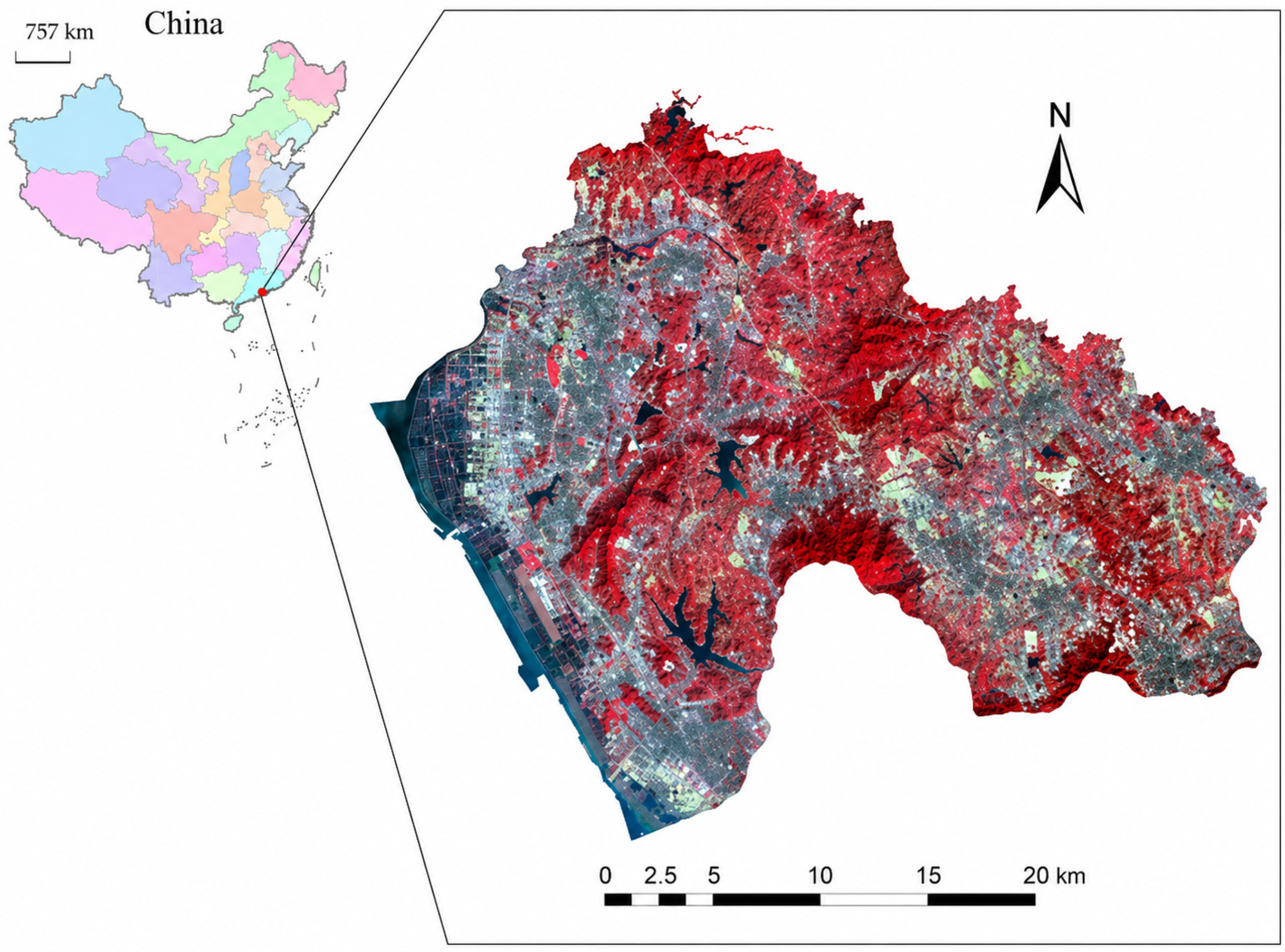
The research utilized Landsat 7 ETM+ imagery (path: 122, row: 44) acquired on 1 January 2003, with minimal cloud cover. The study area, depicted in Figure 1, is situated in Baoan district, Shenzhen, China, covering approximately 733.352 km², with a central coordinate of 113°52′E, 22°35′N. The chosen land cover types were well-suited for our research due to the rapid urban expansion during that period, leading to significant emergence of bare lands for new construction surrounding the city.

By leveraging high-resolution imagery from Google Earth, a local land use map from 2003, and the panchromatic band of the remote sensing image under study, we interpreted 245.991 km² of built-up area, 50.557 km² of bare land, and 436.804 km² of other land uses as reference data, which were then converted into raster format with a resolution of 30 m. To mitigate variations arising from lighting and atmospheric conditions, the remote sensing image underwent correction using the FLASSH module of ENVI 5.3 software.

In order to broaden the applicability of the proposed methods and verify their generalizability, we selected three typical cities—Beijing, Xian, and Guangzhou—located in the north, west, and south of China, respectively, for verification. The remote sensing images were obtained from different Landsat satellites at various times, as indicated in

Table 1. Landsat data used for verification.

Verification Region	Platform	Sensor	Acquisition Date
Xian	Landsat 5	TM	11 January 2011
Beijing	Landsat 7	ETM+	25 May 2003
Guangzhou	Landsat 8	OLI	3 January 2015

. The acquisition dates were selected according to image availability, low cloud contamination, and the presence of representative land-cover types in each city. These scenes include built-up areas, bare land, vegetation, and water bodies with clear spectral differences, thereby providing suitable conditions for evaluating the applicability of the proposed method across different urban environments and Landsat sensors.

3. Methodology

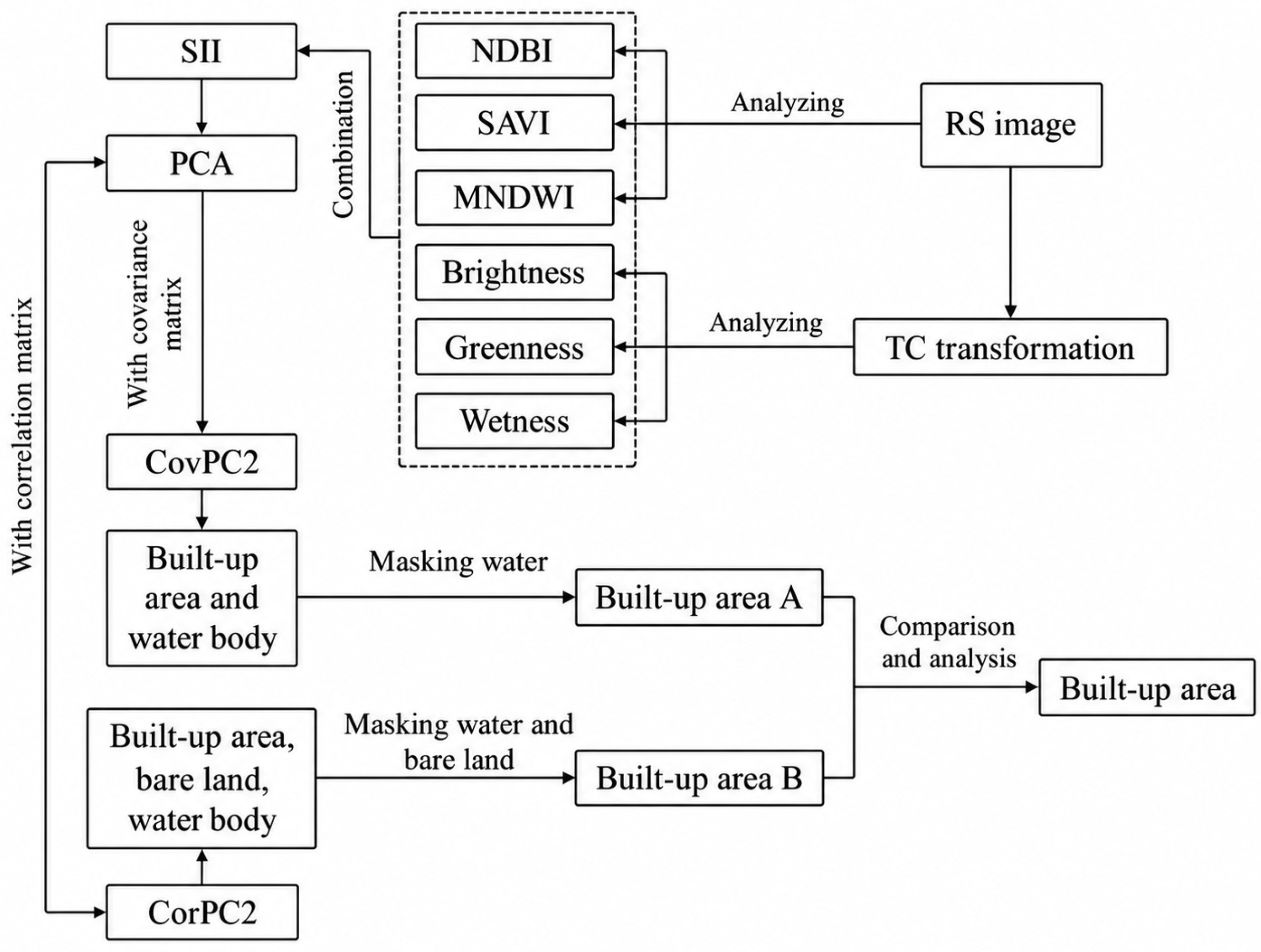
Compared to built-up area extraction index models that rely on the special expression of band calculation, the composition of a multi-index model offers more advantages in extracting the built-up area [37,38,39]. Figure 2 represents a diagram of the built-up area extraction in this research. Initially, the images of NDBI, SAVI, MNDWI, and the components of the Tasseled Cap transformation were overlaid to create a multi-band image (identified as the six indexes image, SII). Subsequently, the PCA method was applied to this image using two different matrices, namely the correlation matrix and the covariance matrix. Following the PCA, the second component was utilized to extract the built-up area. Here, the second component of the covariance matrix-based PCA was referred to as CovPC2, while the second component of the correlation matrix-based PCA was referred to as CorPC2. Considering its stronger ability to suppress bare-land information, CovPC2 was regarded as the main extraction branch, whereas CorPC2 was retained as a comparative variant requiring an additional bare-land mask. Afterwards, a mask was applied to eliminate bare land and water bodies separately, resulting in Built-up Area A and Built-up Area B. Finally, an analysis and comparison were conducted on the extraction results of these two built-up areas to evaluate the performance and applicability of the CovPC2 and CorPC2 methods.

3.1. Composition of Multi Indices

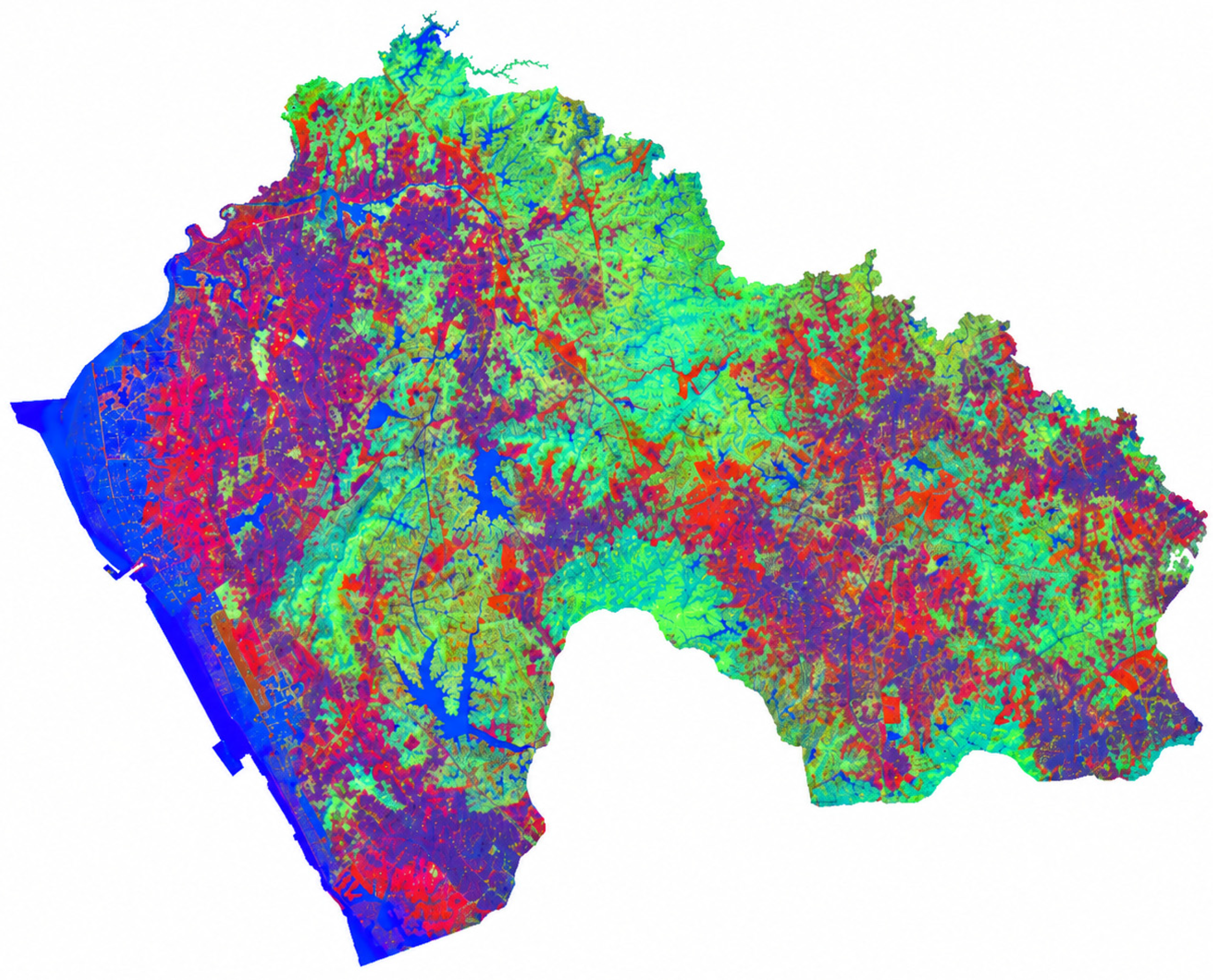
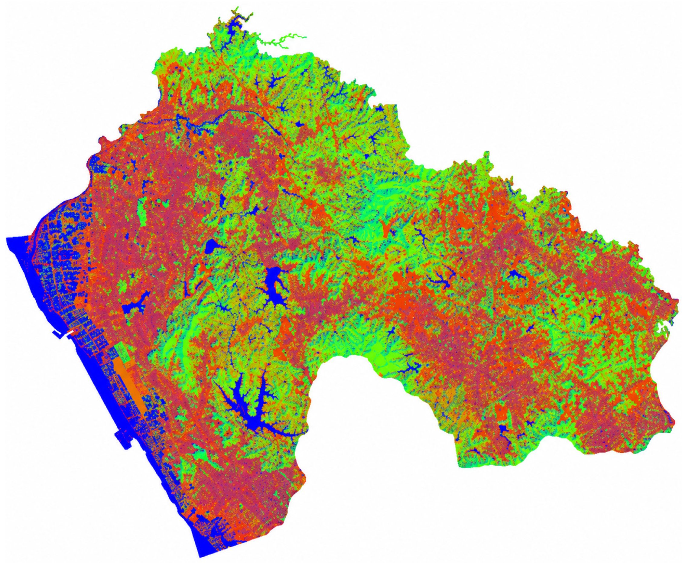
To enhance the contrast between different features, a multi-band image was created by combining images analyzed using different index models in the study. By utilizing various band combinations, certain features could be easily identified. Specifically, urban land use types can be broadly categorized into three groups: built-up areas, vegetation, and water bodies. These categories were represented by NDBI, SAVI, and MNDWI, respectively. This approach reduced data redundancy and spectrum confusion in remote sensing images, while enhancing the separability of different features [40]. Figure 3 illustrates the RGB image overlayed in the order of “NDBI, SAVI, MNDWI” (abbreviated as NSM image). It is evident that built-up areas, bare land, vegetation, and water bodies are assigned distinct colors due to their pronounced differences in each band of the multi-band image.

While the NSM image effectively reveals variations in land use, vegetation, and water bodies, the distinction between bare land and built-up areas is not very pronounced. To enhance this differentiation, we employed the Tasseled Cap (TC) transformation to extract information on soil brightness, vegetation greenness, and moisture levels from the remote sensing imagery. TC transformation is a technique that not only eliminates redundant information among the bands of the original remote sensing image but also captures the information of brightness, greenness, and wetness [41,42]. Built-up areas and bare land are characterized by high intensity, while greenness indicates the distribution of vegetation, and wetness represents factors related to moisture [43,44]. We overlay these three components in the order of “brightness–greenness–wetness” (referred to as BGW imagery) and display them in the form of RGB false color, as shown in Figure 4. It can be observed that in the BGW imagery, bare land is highlighted in red, while other features such as vegetation and water bodies are also enhanced.

The NSM image and BGW image contain rich information for enhancing different land features. To facilitate the analysis and utilization of the differences between various indices, this study combines these two images to create a new image with six bands (SII).

3.2. Dimension Reduction

The different bands of the SII contain enhanced information for built-up areas, bare land, vegetation, water bodies, and other features, as well as some redundant information. To reduce the complexity of the data and effectively separate the enhanced features, spatial dimensionality reduction is required for the multidimensional data. PCA is currently one of the most effective methods for spatial dimensionality reduction [45,46]. This method primarily removes the correlation between bands by rotating the spectral spatial coordinate axes and concentrates the main information into the first 2–3 principal components. This allows for the concentration of useful information from the multi-band image into as few principal component images as possible, ensuring that these component images are mutually independent and effectively reducing the impact of noise [45,46,47].

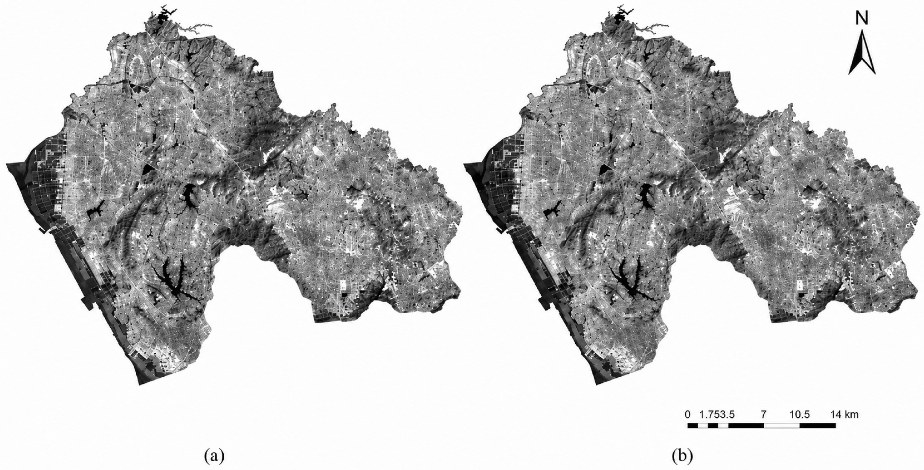
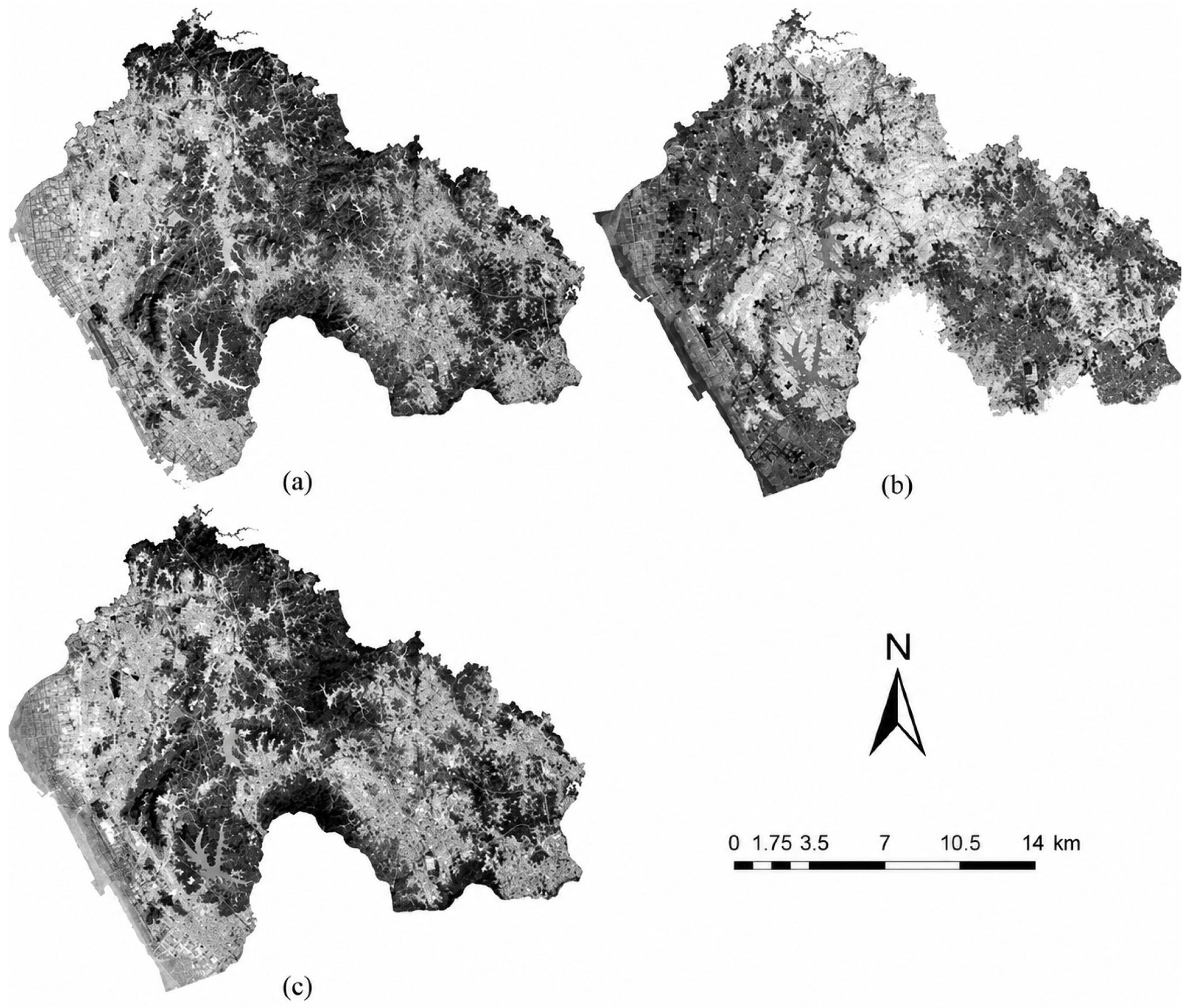
Based on this, the experiment performed PCA on the 6-band image using both the correlation matrix and the covariance matrix. The objective was to concentrate the primary information contained in the image into the first two principal components. Through analysis, it was observed that in the first principal component, the bare land was effectively isolated and enhanced (as shown in Figure 5). This indicates that the first principal component mainly represents the dominant variance related to bare land and brightness information in the multi-index image, rather than the contrast most useful for built-up area extraction. The second principal component was therefore further analyzed because it is orthogonal to the first component and can retain the remaining contrast information among built-up areas, bare land, vegetation, and water bodies. For the covariance-matrix PCA result, both urban areas and water bodies were enhanced in the second principal component, while other land cover types were mostly suppressed, as shown in Figure 6a; this image was referred to as CovPC2. In contrast, for the correlation-matrix PCA result, urban areas, water bodies, and bare land appeared as dark gray in the second principal component, as shown in Figure 6b. To facilitate experimental comparison, Figure 6b was inverted by multiplying it by −1 to obtain Figure 6c, which was referred to as the CorPC2 image.

The difference between CovPC2 and CorPC2 is mainly related to the different treatments of variance in covariance-matrix PCA and correlation-matrix PCA. Covariance-matrix PCA retains the original variance differences among the input indices and components, so features with stronger contrast in the multi-index image have greater influence on the principal components. In contrast, correlation-matrix PCA standardizes all input variables to unit variance, giving different indices more balanced contributions; therefore, part of the bare-land response may still remain in CorPC2, whereas CovPC2 can suppress bare land more effectively in this study.

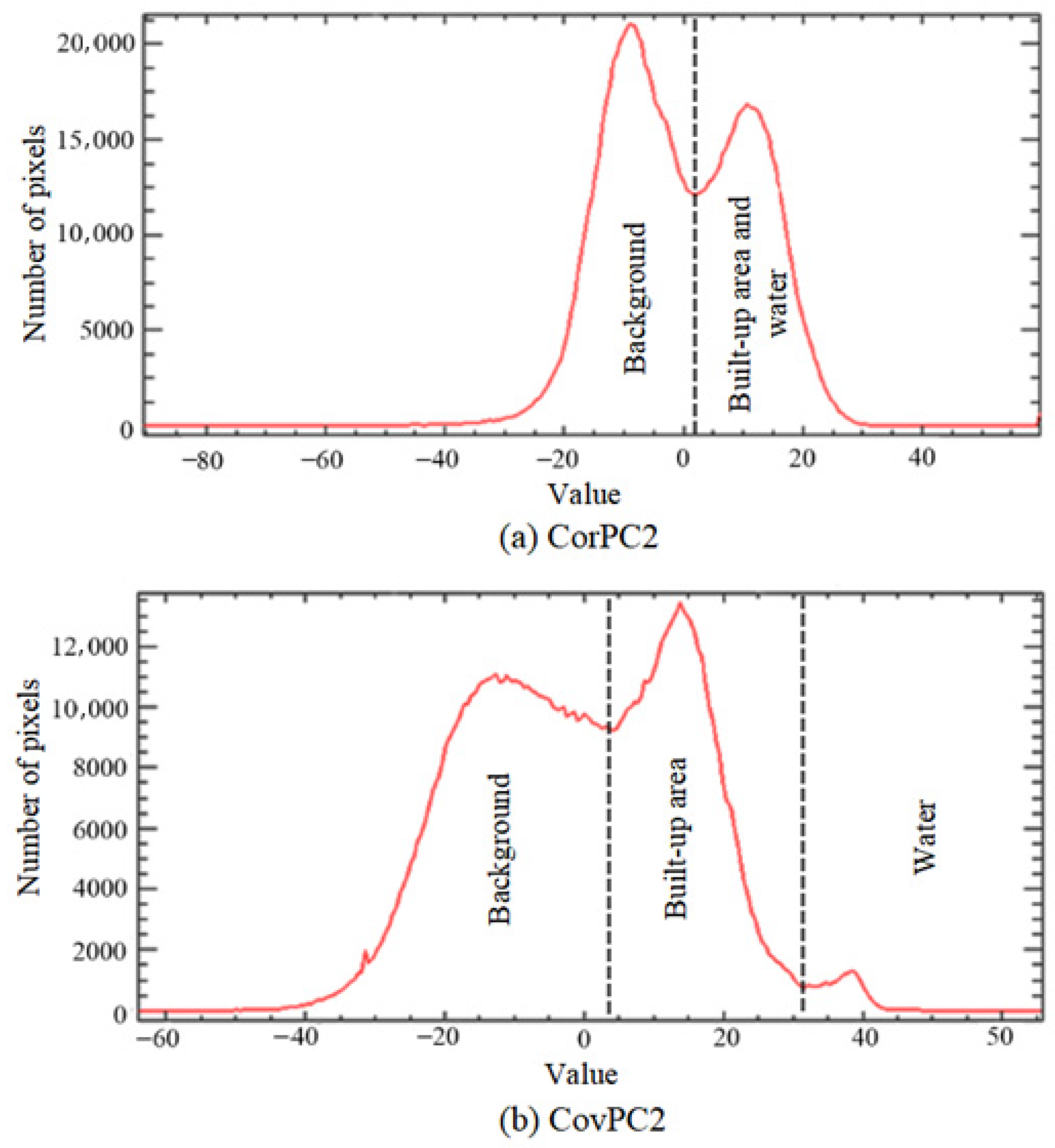
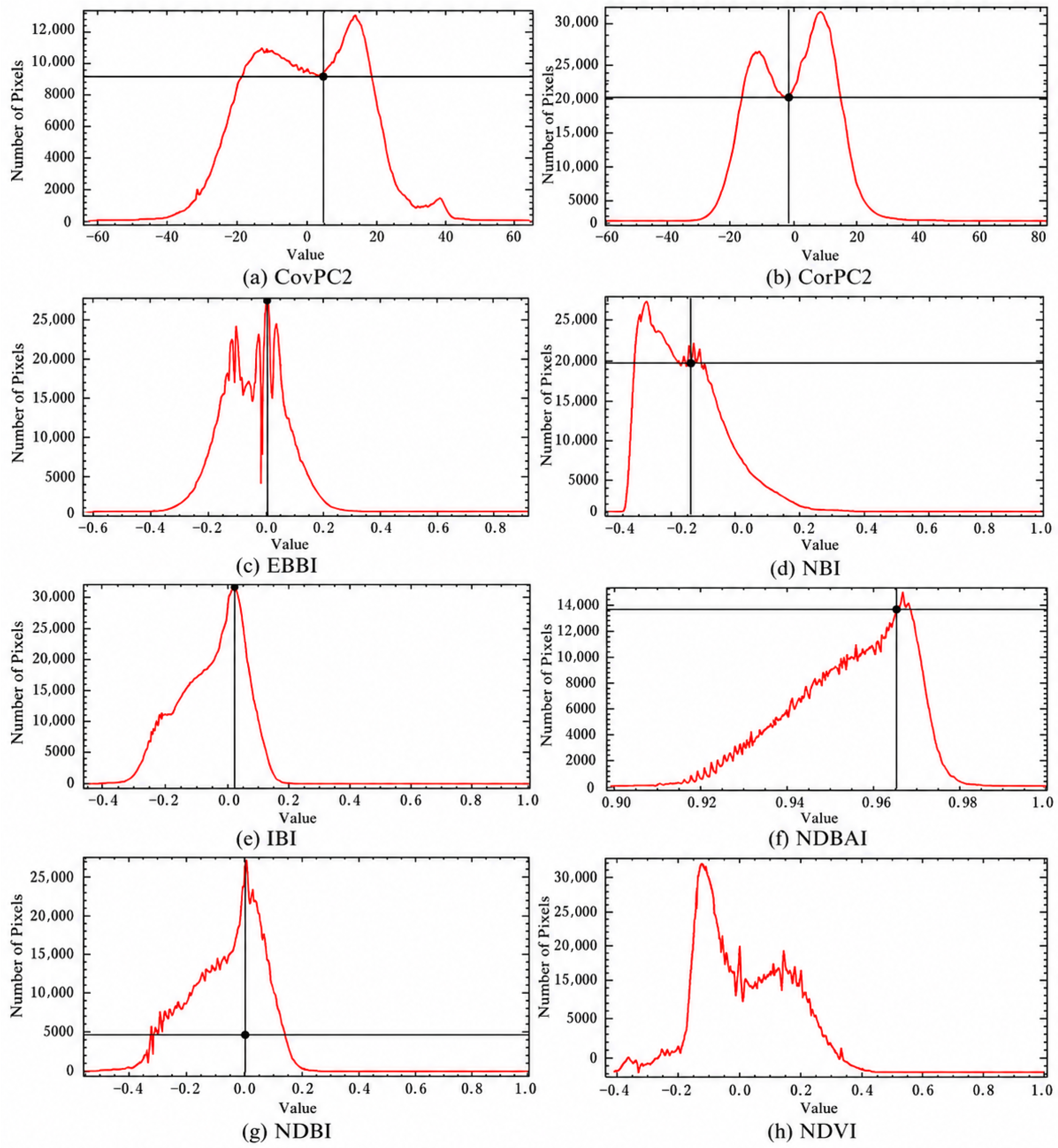
Figure 7 presents the grayscale statistical histograms of the CorPCA2 and CovPCA2 images. It is evident that there are distinct valleys between the enhanced land cover and the background, indicating a high separability between the enhanced land cover and other land cover types in the second principal component derived from the PCA transformation of the SII.

3.3. Water and Bare Land Mask Building

Due to the enhancement of the water body in the CovPC2 image and CorPC2 image, a mask is generated to exclude the water body area. MNDWI is an index model used for extracting water bodies by modifying the band combination of NDWI [40]. This index effectively minimizes the influence of shadows and vegetation. By applying Equation (1), an MNDWI image is obtained, and then, based on the conditional argument provided in Equation (2), the MNDWI image is converted into a binary image, MNDWIB. The expressions for Equations (1) and (2) are as follows:

$$\mathrm{M}\mathrm{N}\mathrm{D}\mathrm{W}\mathrm{I}={\displaystyle \frac{\mathrm{T}\mathrm{M}2-\mathrm{T}\mathrm{M}5}{\mathrm{T}\mathrm{M}2+\mathrm{T}\mathrm{M}5}}$$

(1)

if MNDWI > 0 then MDBWIB = 1 else MDBWIB = 0

(2)

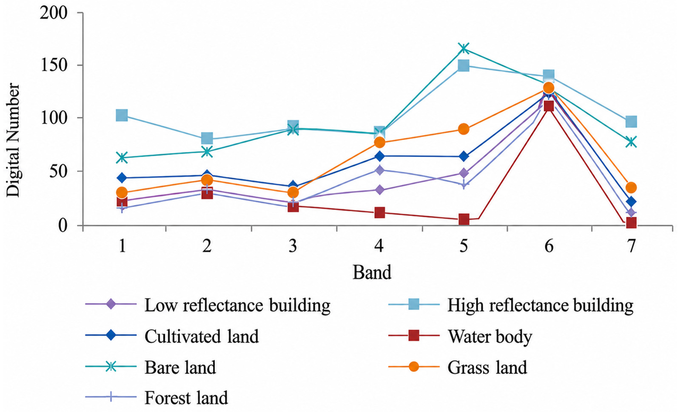
An index model is typically used to mask bare land in the CorPC2 image. However, existing bare land index models often misclassify high-reflectance buildings as bare land due to the lack of consideration for spectral similarity between the two. In order to accurately identify bare land while excluding the effects of high reflectance buildings, we propose a novel index model called the Bareness Area Index (BAI). This model is developed by analyzing the spectral signatures of various land use types, as shown in Figure 8. The DN (Digital Number) value of bare land is higher than that of high reflectance buildings and other land use types in TM band 1 and TM band 2. On the other hand, high reflectance buildings are characterized by a higher DN value in TM band 5. Therefore, TM1 and TM2 were combined to represent the short-wavelength response of bare land, and their sum was used to reduce the uncertainty caused by a single visible band. The contrast between TM5 and (TM1 + TM2) was then used to distinguish bare land from high-reflectance buildings. Consequently, the enhancement of bare land can be achieved by applying the formula (TM5 − (TM1 + TM2))/(TM5 + (TM1 + TM2)). Additionally, to mitigate the influences of vegetation and water bodies, the Soil-Adjusted Vegetation Index (SAVI) and MNDWI can be subtracted. Here, SAVI and MNDWI were subtracted to reduce the interference of sparse vegetation and water bodies, respectively. Since bare land generally has lower vegetation and water-index responses than vegetation and water bodies, this subtraction is not expected to over-suppress bare land. Other commonly used indices, such as NDVI and NDWI, were also considered for representing vegetation and water bodies. However, SAVI was selected because it can reduce the influence of soil background in areas with sparse vegetation, while MNDWI was selected because it enhances water bodies and suppresses built-up land more effectively than conventional NDWI. The equations for BAI and SAVI are as follows:

$$\mathrm{B}\mathrm{A}\mathrm{I}={\displaystyle \frac{\mathrm{T}\mathrm{M}5-(\mathrm{T}\mathrm{M}1+\mathrm{T}\mathrm{M}2)}{\mathrm{T}\mathrm{M}5+(\mathrm{T}\mathrm{M}1+\mathrm{T}\mathrm{M}2)}}-\mathrm{S}\mathrm{A}\mathrm{V}\mathrm{I}-\mathrm{M}\mathrm{N}\mathrm{D}\mathrm{W}\mathrm{I}$$

(3)

if BAI > T then BAIB = 1 else BAIB = 0

(4)

$$\mathrm{S}\mathrm{A}\mathrm{V}\mathrm{I}={\displaystyle \frac{\left(\mathrm{T}\mathrm{M}4-\mathrm{T}\mathrm{M}3\right)+(1+l)}{\mathrm{T}\mathrm{M}4+\mathrm{T}\mathrm{M}3+l}}$$

(5)

where T is the optimal threshold for BAI image segmentation; BAIB is the binary result of BAI image segmentation; l is a constant between 0 and 1, its default value is 0.5.

3.4. Built Up Area Extraction

Before extracting the built-up area, the enhanced features are first separated from their background. In Figure 7, the CorPC2 image and CovPC2 image exhibit a strong contrast between the enhanced features and their background, resulting in a typical double peak in their histograms. One peak represents the enhanced features, while the other corresponds to the background. By leveraging the histogram with a double peak, a threshold can be automatically selected. The Otsu method, a widely used image segmentation algorithm, determines the threshold by analyzing the distribution of peaks in the image’s gray histogram [48]. Its effectiveness has been well-established through years of research and experimentation [49,50]. In this study, we applied the Otsu method to the gray histograms of the CorPC2 image and CovPC2 image to automatically select the threshold. The algorithmic procedure can be found in [48]. The equations for extracting the enhanced features are as follows.

If PC2Cor > TCor then ExtCor = 1 else ExtCor = 0,

(6)

If PC2Cov > TCov then ExtCov = 1 else ExtCov = 0,

(7)

where PC2Cor and PC2Cov represent the pixels value of CorPC2 image and CovPC2 image, respectively; TCor and TCov are the threshold calculated by Ostu algorithm; ExtCor and ExtCov are the binarized outputs after segmentation of CorPC2 image and CovPC2 image.

Finally, after masking the water bodies in the CorPC2 and CovPC2 images, as well as the bare land in the CorPC2 image, the process for extracting the built-up areas is as follows:

BACor = ExtCor − MNDWIB,

(8)

BACor = ExtCor − MNDWIB − BAIB.

(9)

Here, BACov and BACor represent the binary images where 1 is assigned to built-up areas and 0 to non-built-up areas. In this paper, we refer to the built-up area extraction method using the CovPC2 image as the CovPC2 method and the method using the CorPC2 image as the CorPC2 method.

4. Experiment and Results

In order to assess the effectiveness of built-up area extraction methods using CorPC2 and CovPC2 images, the results were compared with those obtained from existing index models such as IBI, NDBI, NBI, NBAI, and EBBI. The equations for these models are as follows.

$$\mathrm{N}\mathrm{D}\mathrm{B}\mathrm{I}={\displaystyle \frac{\mathrm{T}\mathrm{M}5-\mathrm{T}\mathrm{M}4}{\mathrm{T}\mathrm{M}5+\mathrm{T}\mathrm{M}4}}$$

(10)

$$\mathrm{N}\mathrm{B}\mathrm{I}={\displaystyle \frac{\mathrm{T}\mathrm{M}3\cdot \mathrm{T}\mathrm{M}5}{\mathrm{T}\mathrm{M}4}}$$

(11)

$$\mathrm{N}\mathrm{B}\mathrm{A}\mathrm{I}={\displaystyle \frac{\mathrm{T}\mathrm{M}7-\mathrm{T}\mathrm{M}5/\mathrm{T}\mathrm{M}2}{\mathrm{T}\mathrm{M}7-\left(\mathrm{T}\mathrm{M}5/\mathrm{T}\mathrm{M}2\right)}}$$

(12)

$$\mathrm{E}\mathrm{B}\mathrm{B}\mathrm{I}={\displaystyle \frac{\mathrm{T}\mathrm{M}5-\mathrm{T}\mathrm{M}4}{10\sqrt{\mathrm{T}\mathrm{M}5+\mathrm{T}\mathrm{M}6}}}$$

(13)

A progressive search method was utilized to determine the optimal threshold for extracting built-up areas or bare land for accuracy evaluation. Initially, the maximum and minimum values of each image were calculated, and then the range was divided into N equal parts to establish the search step. Subsequently, the optimal threshold was determined by accumulating the search step from the minimum value. The threshold value (T) can be calculated using Formula (14).

$$\mathrm{T}=\mathrm{M}\mathrm{i}\mathrm{n}+\mathrm{i}\ast \left(\mathrm{M}\mathrm{a}\mathrm{x}-\mathrm{M}\mathrm{i}\mathrm{n}\right)/\mathrm{N}$$

(14)

where i is an integer ranging from 0 to N. With N set as 1000, the threshold for each image segmentation was optimized incrementally. The transition matrix from the extraction result to the reference data was then computed to determine the producer’s accuracy and user’s accuracy. A higher producer’s accuracy and user’s accuracy indicate a greater correspondence between the extracted result and its reference. The producer’s accuracy and user’s accuracy for built-up areas or bare land using the CorPC2 method, CovPC2 method, and other existing index model methods are listed in

Table 2. Accuracy of built-up areas and bearland extracted by different methods.

	Methods	PA (%)	UA (%)	F1 (%)	IoU (%)	OA (%)
Built-up areas	IBI	80.92	75.97	78.37	64.43	85.01
	NDBI	66.19	79.69	72.32	56.64	83.00
	NBI	66.72	83.61	74.22	59.00	84.45
	NBAI	81.23	58.49	68.01	51.53	74.37
	EBBI	66.86	72.77	69.69	53.48	80.49
	CorPC2Opt	83.66	90.18	86.80	76.67	91.46
	CorPC2Otsu	82.98	89.33	86.04	75.50	90.97
	CovPC2Opt	91.09	96.57	93.75	88.24	95.93
	CovPC2Otsu	90.00	95.88	92.85	86.65	95.35
Bare land	IBI	71.55	76.62	74.00	58.73	96.53
	NDBI	58.56	66.32	62.20	45.14	95.09
	NBI	65.28	78.90	71.45	55.58	96.40
	NBAI	4.99	5.77	5.35	2.75	87.83
	EBBI	62.21	69.68	65.73	48.96	95.53
	BAI	90.99	87.29	89.10	80.35	98.47

Note: PA, UA, F1, IoU, and OA represent Producer’s Accuracy, User’s Accuracy, F1-score, Intersection over Union, and Overall Accuracy, respectively.

(CovPC2Opt and CovPC2Opt refer to the thresholds Tcor and Tcov in Equation (6) and Equation (7), respectively, which were obtained using a gradual search method. CovPC2Otsu and CovPC2Otsu indicate that the thresholds in Equations (6) and (7) were calculated using the Otsu algorithm).

To further examine the influence of the BAI mask on the CorPC2 method, the intermediate CorPC2 result after water removal only was also evaluated. Compared with this intermediate result, the final CorPC2 result after both water and bare-land removal showed (changes in PA, UA, F1, IoU, and OA), indicating that the BAI mask reduced bare-land commission errors but also introduced some uncertainty due to omission and commission errors in bare-land extraction.

As shown in Table 2, the proposed CovPC2 and CorPC2 methods outperformed the conventional built-up indices in terms of both producer’s accuracy and user’s accuracy. Among all methods, CovPC2Opt achieved the best performance, with a producer’s accuracy of 91.09% and a user’s accuracy of 96.57%, followed closely by CovPC2Otsu with 90.00% and 95.88%, respectively. The CorPC2 method also yielded strong results, with producer’s accuracies above 82% and user’s accuracies around 89–90%, which were consistently higher than those of the conventional indices. Moreover, the derived evaluation metrics further confirmed these advantages: CovPC2Opt achieved the highest F1-score (93.75%), IoU (88.24%), and approximate OA (95.93%), while CovPC2Otsu ranked second with an F1-score of 92.85%, an IoU of 86.65%, and an approximate OA of 95.35%. Similarly, CorPC2Opt and CorPC2Otsu achieved F1-scores of 86.80% and 86.04%, IoU values of 76.68% and 75.50%, and approximate OA values of 91.46% and 90.97%, respectively. In addition, although the two peaks in the gray histograms were not completely symmetrical, the Otsu-based extraction results were highly consistent with those obtained using the gradual-search optimal threshold. For CovPC2, the differences in PA and UA between CovPC2Opt and CovPC2Otsu were only 1.09 and 0.69 percentage points, respectively. For CorPC2, the corresponding differences were 0.68 and 0.85 percentage points. This consistency indicates that Otsu can provide a reliable automatic threshold for the proposed PC2 images in this study.

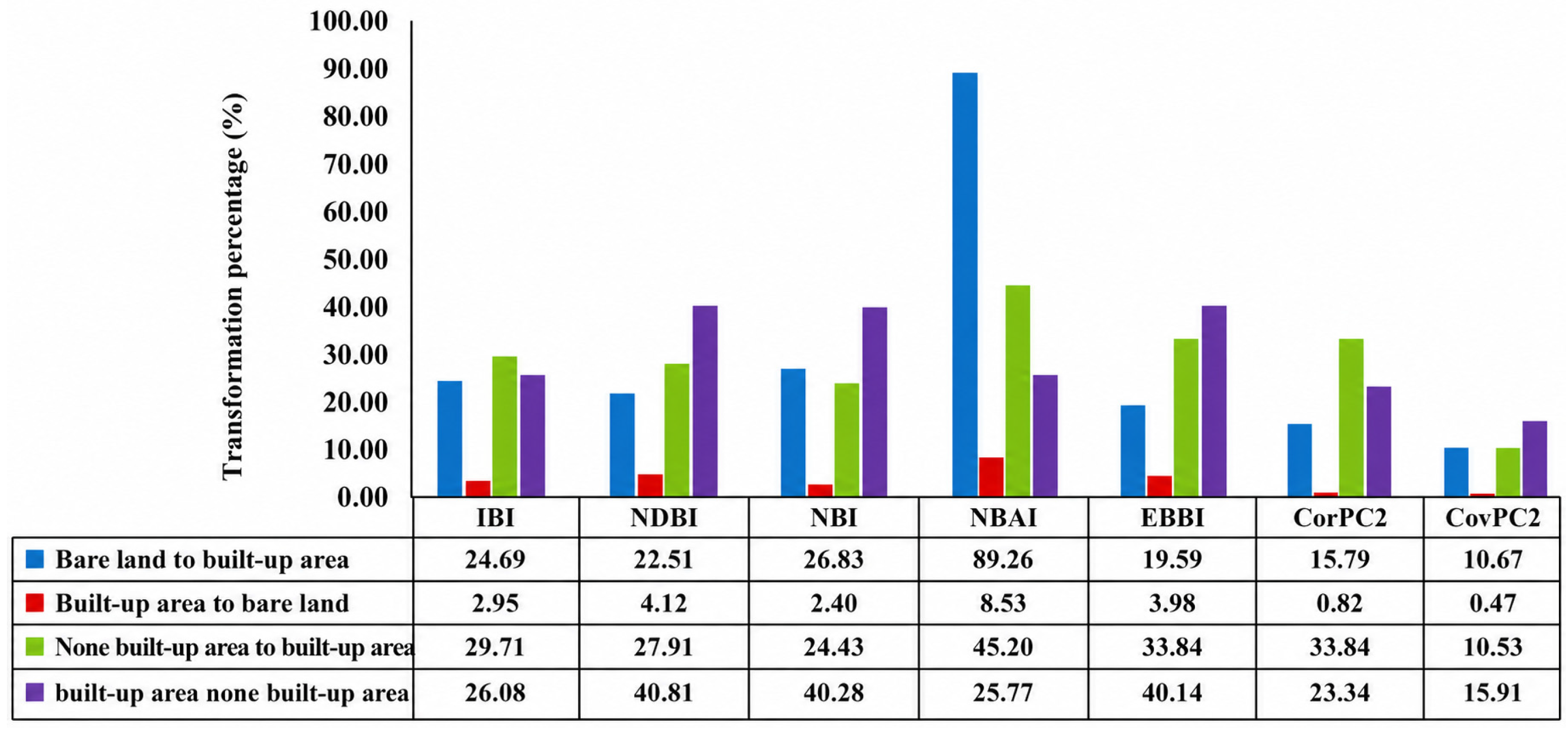
Figure 9 illustrates the error rates between built-up areas and bare land, as well as between built-up areas and non-built-up areas. It is evident that when using the CorPC2 method and CovPC2 method, the misclassification rates of bare land and built-up areas were significantly lower compared to other index methods, demonstrating their strong capability in identifying bare land and built-up areas. Similarly, the misclassification rate between built-up areas and non-built-up areas was lower when using the CorPC2 method and CovPC2 method compared to other index methods. The CovPC2 method exhibited a lower rate of misclassification in this regard than the CorPC2 method, likely because the CovPC2 method effectively suppressed almost all bare land information. Conversely, when using the BAI to eliminate bare land in the CorPC2 image, some errors were introduced. Overall, the CovPC2 method demonstrated higher accuracy in built-up area extraction compared to the CorPC2 method. This is consistent with the accuracy assessment of BAI in Table 2, where BAI achieved a PA of 90.99% and a UA of 87.29% for bare-land extraction; although these values indicate good bare-land identification ability, the remaining omission and commission errors can still propagate into the final CorPC2 result.

In order to further verify whether the performance differences among methods were statistically meaningful, a pixel-wise paired significance analysis was conducted for the experiment as shown in

Table 3. Statistical significance analysis for pairwise comparison of built-up area extraction methods in the experiment.

Comparison	b (A Correct, B Wrong)	c (A Wrong, B Correct)	Chi-Square (cc)	p-Value	Significant (α = 0.05)
CovPC2 vs. CorPC2	39,977	19,210	7285.8357	<0.001	Yes
CovPC2 vs. EBBI	162,921	36,123	80,773.4933	<0.001	Yes
CovPC2 vs. NBAI	749,230	42,079	631,941.6593	<0.001	Yes
CovPC2 vs. NBI	139,197	28,078	73,813.8390	<0.001	Yes
CovPC2 vs. NDBI	739,941	38,091	633,125.6540	<0.001	Yes
CorPC2 vs. EBBI	137,275	31,244	66,712.7202	<0.001	Yes
CorPC2 vs. NBAI	739,842	53,458	593,875.7377	<0.001	Yes
CorPC2 vs. NBI	102,130	11,778	71,665.7583	<0.001	Yes
CorPC2 vs. NDBI	738,236	57,153	583,202.2956	<0.001	Yes

Note: Chi-square uses McNemar’s test with continuity correction; p-value computed as right-tail probability of χ² with 1 d.f.

. Since all methods were evaluated against the same reference map, McNemar’s test was adopted for pairwise comparison using the discordant classifications between each pair of methods. The significance testing results showed that the proposed CovPC2 method significantly outperformed all comparison methods, including CorPC2, EBBI, NBAI, NBI, and NDBI (ρ < 0.001). In addition, CorPC2 also significantly outperformed EBBI, NBAI, NBI, and NDBI (ρ < 0.001). These results provide statistical evidence that the PCA-based methods achieved clear advantages over the conventional index-based approaches for built-up area extraction. This finding is consistent with the accuracy results in Table 2, where CovPC2Opt and CorPC2Opt achieved higher producer’s accuracy and user’s accuracy than the traditional indices.

Considering the large number of evaluated pixels, relative percentage improvements were further calculated to indicate the practical magnitude of the accuracy differences. Taking the best conventional-index result as the baseline, CovPC2Opt improved the F1-score, IoU, and OA by 15.38, 23.81, and 10.92 percentage points, corresponding to relative improvements of 19.62%, 36.95%, and 12.85%, respectively. CorPC2Opt improved the corresponding metrics by 8.43, 12.24, and 6.45 percentage points, corresponding to relative improvements of 10.76%, 19.00%, and 7.59%, respectively. These improvements indicate that the statistical significance shown in Table 3 corresponds to meaningful accuracy gains rather than only to the large sample size.

Figure 10 displays the gray-level histograms of the CorPC2 image, CovPC2 image, and other images analyzed by IBI, NDBI, NBI, NBAI, EBBI, and NDVI (NDVI was used for comparison purposes). When using the existing index models, the built-up area was enhanced, but it was challenging to achieve a sharp contrast between the built-up area and its background. As shown in the gray histogram of the NDVI image in Figure 10, both the enhanced feature and its background have their own peaks, and vegetation could be separated with a threshold near zero. In contrast to NDVI, the existing built-up area index models lack a fixed threshold for image segmentation, making it difficult to find the best threshold automatically. Therefore, the progressive-search optimal threshold was used for these conventional indices to provide their best possible binarization results, which makes the comparison with the proposed automatic Otsu-based PC2 methods conservative rather than favorable to the proposed methods. Similarly, in the gray histograms of the CovPC2 image, a distinct trough appears due to the high degree of separation between the enhanced feature and its background, indicating that a threshold could be optimized using a typical algorithm. Furthermore, the smooth and delicate incurves in both the gray histograms of the CorPC2 image and CovPC2 image were quite different from the zigzagged incurves of the existing index model images, suggesting that the noises were effectively filtered by the CovPC2 method and CorPC2 method after principal component analysis.

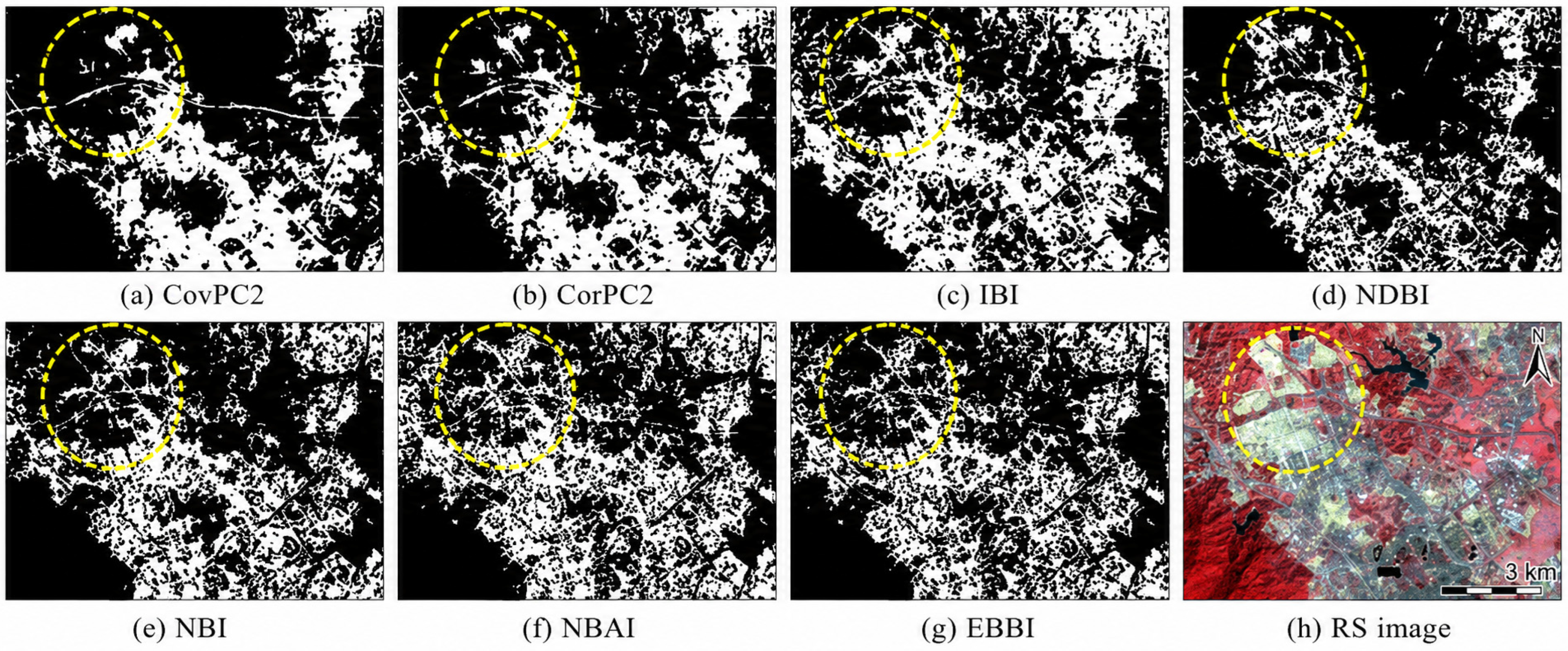
The built-up area extraction results are depicted in Figure 11, clearly demonstrating that the extracted built-up areas were more regular and homogeneous when using the CorPC2 method and CovPC2 method compared to other existing index methods. These methods effectively removed bare land, resulting in higher overall accuracy. Specifically, the CovPC2Opt method achieved PA, UA, F1-score, IoU, and OA values of 91.09%, 96.57%, 93.75%, 88.24%, and 95.93%, respectively, while the CorPC2Opt method achieved corresponding values of 83.66%, 90.18%, 86.80%, 76.67%, and 91.46%. These quantitative results further support the visual comparison shown in Figure 11. Additionally, most buildings with high reflectance were correctly recognized as built-up areas, leading to a decrease in confusion with bare land.

5. Discussion

5.1. Feature Enhance Analysis

Table 4. Correlation coefficient among NDBI, SAVI, MNDWI, brightness, greenness, and wetness.

	NDBI	SAVI	MNDWI	Brightness	Greenness	Wetness
NDBI	1.000	−0.293	−0.625	0.684	−0.441	−0.700
SAVI	−0.293	1.000	−0.461	−0.093	0.951	−0.282
MNDWI	−0.625	−0.461	1.000	−0.691	−0.271	0.946
Brightness	0.684	−0.093	−0.691	1.000	−0.327	−0.784
Greenness	−0.441	0.951	−0.271	−0.327	1.000	−0.105
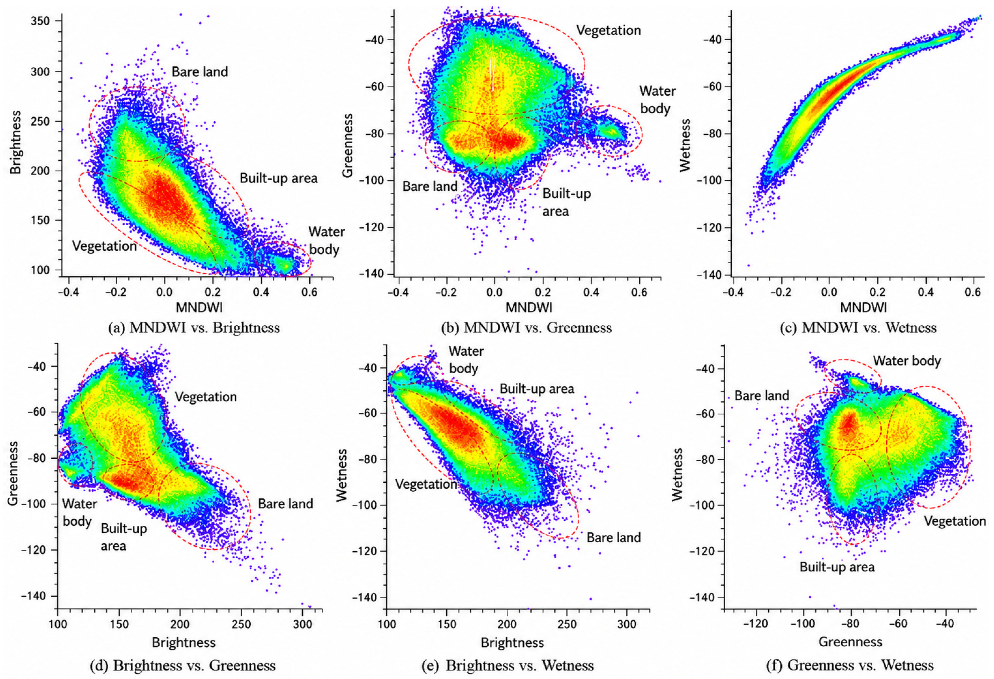
Wetness	−0.700	−0.282	0.946	−0.784	−0.105	1.000

presents the correlation coefficients between the six bands of the SII. It can be observed that, except for SAVI and Greenness, MNDWI shows a high correlation with Wetness (correlation coefficients of 0.951 and 0.946, respectively). The correlation coefficients between other indices (or components) are relatively low, indicating a high degree of independence between these indices (or components) and a strong contrast among them. The relatively high correlations between SAVI and Greenness and between MNDWI and Wetness indicate partial redundancy among the six input layers, which further supports the use of PCA to transform correlated variables into mutually orthogonal principal components and reduce redundant information.

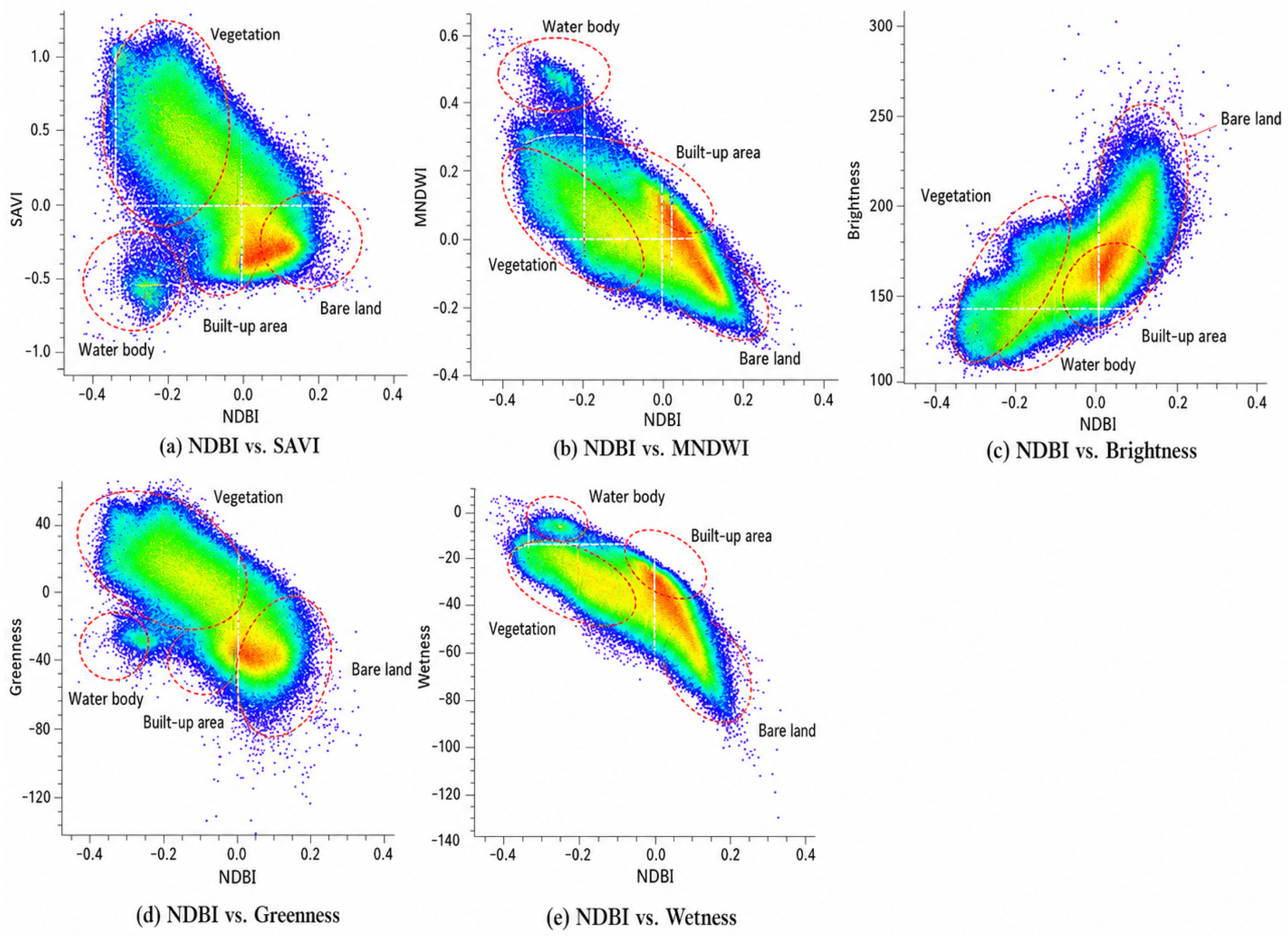
In the scatterplots of the NDBI image versus the MNDWI image (Figure 12b) and the NDBI image versus the wetness image (Figure 12e), the distribution of bare land, built-up areas, and vegetation towards the vertex direction of the point cluster polygon indicated a higher separability of each class compared to the scatterplots in Figure 12a,c,d. This suggests that the combination of the NDBI image and the MNDWI image, as well as the combination of the NDBI image and the wetness image, could enhance the differences among different classes. Clearly, the enhancement of bare land is evident in the scatterplots shown in Figure 12e.

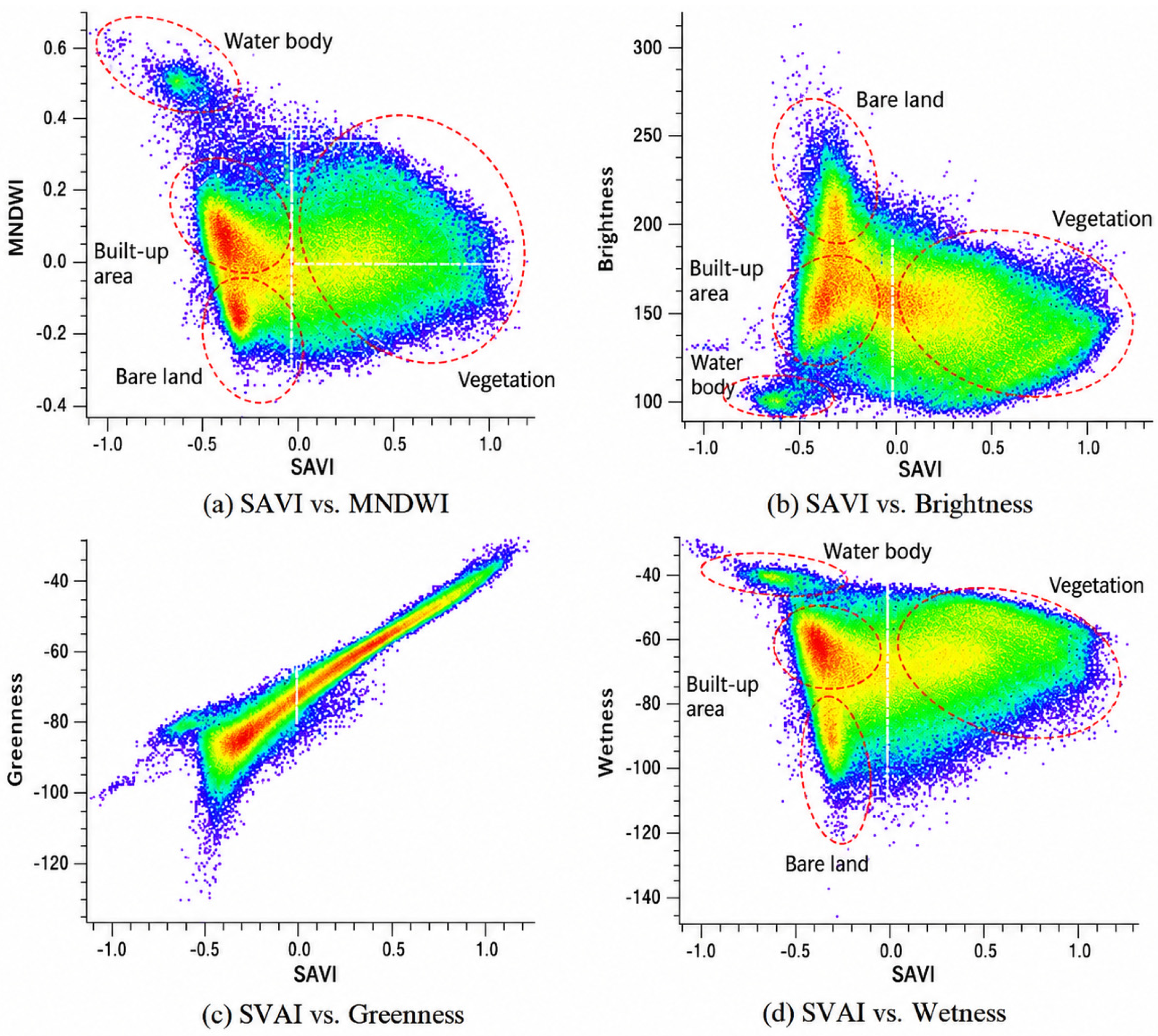
Figure 13a,b,d demonstrate clear separability characteristics, with improved performance in vegetation separation. In Figure 13b, aside from the water body and vegetation regions, the built-up area and bare land were distinctly located on opposite sides of a rugby-ball-like point cluster, indicating a high level of separation between them. Similarly, a triangle-like point cluster is evident in Figure 13d, clearly showing that the points representing built-up areas, bare land, and vegetation were clustered at each corner, thus confirming that the combination of SAVI and wetness enhanced the characteristics of the built-up area, bare land, and vegetation.

The combinations of indexes in Figure 14 were not effective in separating different classes, similar to the results in Figure 10 and Figure 11. However, the water body was effectively distinguished from other features in all cases, as it exhibited distinct characteristics in each index image. Different combinations of index images allowed for varying levels of separation among features such as built-up areas, bare land, water bodies, and vegetation. Nonetheless, not all combinations were suitable for feature enhancement due to the presence of data redundancy (Figure 13c and Figure 14c). Therefore, it is necessary to eliminate data redundancy in the SII to simplify the complexity of built-up area extraction.

5.2. Generalization Analysis

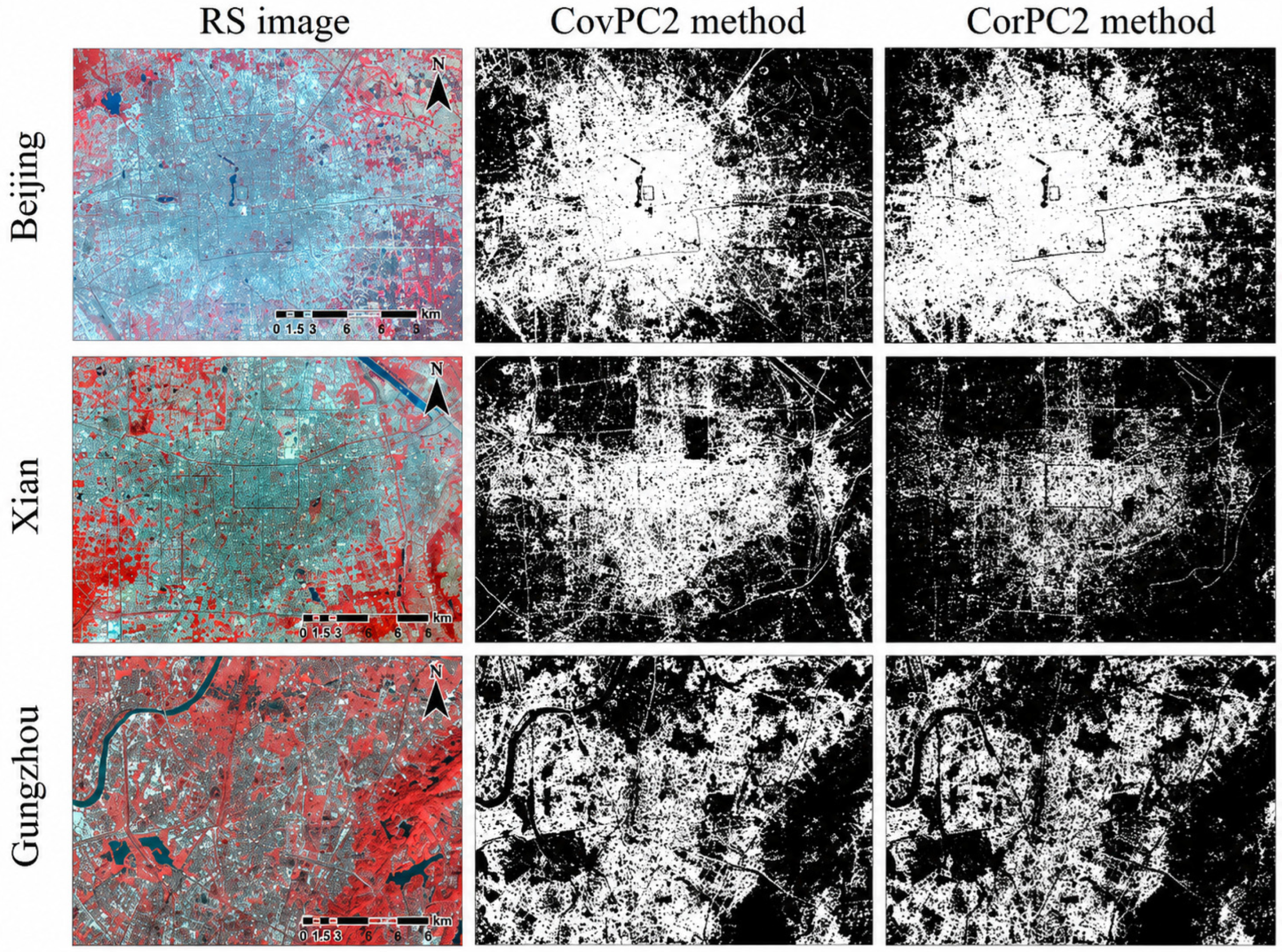
In order to validate the generality of the proposed method in this paper, we utilized the CovPC2 and CorPC2 methods to extract the built-up areas in three regions located in Beijing, Xi’an, and Guangzhou, China. The results of the built-up area extraction with the CovPC2 and CorPC2 methods are presented in Figure 15. The final accuracy evaluation revealed that the built-up area extraction accuracy using the CovPC2 method was 87.13% for Beijing, 88.13% for Xi’an, and 88.13% for Guangzhou. On the other hand, the accuracy using the CorPC2 method was 85.65% for Beijing, 83.35% for Xi’an, and 87.51% for Guangzhou. Overall, the built-up area extraction accuracy with the CovPC2 method was higher than that with the CorPC2 method. It was verified that the accuracy of built-up area extraction would be affected with the CorPC2 method due to errors in eliminating bare land in the CorPC2 image, while bare land was effectively suppressed with the CovPC2 method. This difference was particularly evident in the Xi’an verification region, where the accuracy of CovPC2 reached 88.13%, whereas that of CorPC2 was 83.35%. The main reason is that the CorPC2 image enhances not only built-up areas but also part of the bare land, and therefore an additional BAI-based bare land mask is required. In Xi’an, bare land and sparse vegetation are widely distributed around the urban fringe, and their spectral characteristics are similar to those of some built-up surfaces. As a result, residual bare land or masking errors may occur in the CorPC2 result. In contrast, the CovPC2 method suppresses most bare land information during PCA transformation and therefore produces a cleaner and more stable built-up area extraction result. This explains the more obvious difference between the two methods in Xi’an shown in Figure 15.

Since the index models for generating the SII are common to most remote sensing images from different satellites, these two methods, based on the SII, can also be applied to images obtained by other Landsat sensors. In fact, they demonstrated better performance in extracting the built-up area of Xi’an from TM images and Guangzhou from OLI images with high accuracies. Although Landsat 5 TM, Landsat 7 ETM+, and Landsat 8 OLI have differences in spectral response and radiometric characteristics, the corresponding bands used for calculating NDBI, SAVI, MNDWI, and tasseled cap components have consistent physical meanings. In this study, sensor-specific band combinations and tasseled cap coefficients were used, and all images were preprocessed before index calculation. Therefore, sensor differences may slightly affect the absolute values of the indices and principal components, but they are unlikely to change the relative separability among built-up areas, bare land, vegetation, and water bodies, which is the basis of the proposed method. The validation results from different Landsat sensors further indicate that the proposed method has good cross-sensor applicability.

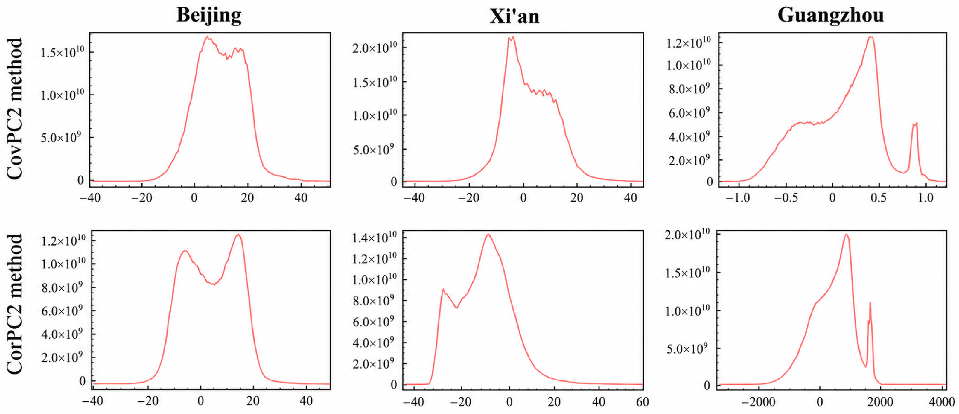
As depicted in Figure 16, the gray level histograms of the CovPC2 and CorPC2 images for each verification area were characterized by distinct peaks, representing enhanced features and backgrounds. It was evident that the enhanced features were clearly separated from the backgrounds in both the CovPC2 and CorPC2 images. The curves in all the histograms were smooth, indicating that the noise was effectively suppressed when PCA was applied to the SIIs. In the histogram of the CovPC2 image for the Guangzhou verification region, a small but distinct peak was observed at the right end of the curve, representing the water body, which was also evident in the CorPC2 image. This indicated a clear separation between the water body and its background in both the CovPC2 and CorPC2 images.

No peaks representing the water body were observed in the gray-level histograms of the CovPC2 images for the Beijing and Xi’an verification regions, as well as the CorPC2 images for these two regions. Upon analyzing the composition and distribution of land use types in these two regions, it was observed that the water body accounted for a very small portion of the total area. The absence of peaks for the water body in the histograms was attributed to the distribution of frequencies being directly related to the proportion of each land use type in the total area. Therefore, it was concluded that a statistical area should be carefully selected to obtain the gray level histograms of the CovPC2 and CorPC2 images for threshold optimization. To enable the proposed method to be applied in a wider area, our suggestion is to first obtain the segmentation thresholds for CovPC2 and CorPC2 images in an area with equal built-up areas, water bodies, and vegetation distribution. Then, apply the obtained segmentation thresholds to the entire Landsat image to ultimately extract built-up areas.

The CovPC2 and CorPC2 images enhance both water bodies and built-up areas, making our proposed CovPC2 and CorPC2 methods potentially sensitive to water bodies. Therefore, we recommend that when water bodies occupy a small area in the region and finding threshold values in the histogram is challenging, using masks generated by MNDWI to eliminate water bodies from the enhanced results of CovPC2 and CorPC2 can be effective for extracting built-up areas. However, if water bodies are widely distributed in the region, optimizing threshold values through histogram analysis would be the most effective way to extract built-up areas, as demonstrated in the southern Chinese cities of Guangzhou and Shenzhen. Considering the above accuracy comparison and practical applicability, the CovPC2 result is recommended as the final built-up area extraction result in practical applications because it showed higher accuracy and better bare-land suppression in the verification experiments, whereas the CorPC2 result can be used as an auxiliary reference.

6. Conclusions

In this paper, we utilized the PCA method to reduce spatial dimensionality and thereby lower the complexity of analysis. We introduced two built-up area methods, namely the CorPC2 method and the CovPC2 method, based on the correlation matrix and covariance matrix, respectively. Subsequently, we derived several key conclusions as follows:

(1) The enhanced features in the second component of the PCA method, when applied to the SII, can effectively extract built-up areas. In the CorPC2 image, built-up areas, bare land, and water bodies were enhanced, while in the CovPC2 image, bare land was effectively suppressed, and built-up areas as well as water bodies were enhanced. The non-built-up areas in the enhanced features could be eliminated using a mask, such as the bare land in the CorPC2 image being erased with the mask produced by BAI.

(2) The high separability led to the appearance of typical twin peaks in the gray histogram of both the CorPC2 and CovPC2 images, which can be utilized to automatically determine the threshold for image segmentation using an algorithm.

(3) In comparison with existing index methods, both the CorPC2 and CovPC2 methods demonstrated higher producer’s accuracy and user’s accuracy. Their strong anti-noise capabilities resulted in more regular and homogeneous built-up area extraction results.

(4) During the built-up area extraction process, the CovPC2 method proved to be more automatic than the CorPC2 method, as it effectively suppressed bare land without the need for manual intervention, unlike the CorPC2 method which utilized a mask produced by BAI for bare land elimination. Although BAI could precisely extract bare land, errors still required manual correction.

(5) Both the CorPC2 and CovPC2 methods effectively identified high reflectivity buildings as built-up areas, demonstrating superior performance in suppressing spectral confusion between built-up areas and bare land when compared to existing index models.

References

1. Wu, H.; Gai, Z.; Guo, Y.; Li, Y.; Hao, Y.; Lu, Z.N. Does environmental pollution inhibit urbanization in China? A new perspective through residents’ medical and health costs. Environ. Res. 2020, 182, 109128. [Google Scholar] [CrossRef]
2. Ren, Z.; Fu, Y.; Dong, Y.; Zhang, P.; He, X. Rapid urbanization and climate change significantly contribute to worsening urban human thermal comfort: A national 183-city, 26-year study in China. Urban Clim. 2022, 43, 101154. [Google Scholar] [CrossRef]
3. Li, W.; Hai, X.; Han, L.; Mao, J.; Tian, M. Does urbanization intensify regional water scarcity? Evidence and implications from a megaregion of China. J. Clean. Prod. 2020, 244, 118592. [Google Scholar] [CrossRef]
4. Wang, Y.; Zhai, J.; Song, L. Waterlogging risk assessment of the Beijing-Tianjin-Hebei urban agglomeration in the past 60 years. Theor. Appl. Climatol. 2021, 145, 1039–1051. [Google Scholar] [CrossRef]
5. Chatterjee, U.; Majumdar, S. Impact of land use change and rapid urbanization on urban heat island in Kolkata city: A remote sensing based perspective. J. Urban Manag. 2022, 11, 59–71. [Google Scholar] [CrossRef]
6. Ma, S.; Cai, Y.; Xie, D.; Zhang, X.; Zhao, Y. Towards balanced development stage: Regulating the spatial pattern of agglomeration with collaborative optimal allocation of urban land. Cities 2022, 126, 103645. [Google Scholar] [CrossRef]
7. Yin, J.; Dong, J.; Hamm, N.A.; Li, Z.; Wang, J.; Xing, H.; Fu, P. Integrating remote sensing and geospatial big data for urban land use mapping: A review. Int. J. Appl. Earth Obs. Geoinf. 2021, 103, 102514. [Google Scholar] [CrossRef]
8. Shao, Z.; Wu, W.; Li, D. Spatio-temporal-spectral observation model for urban remote sensing. Geo-Spat. Inf. Sci. 2021, 24, 372–386. [Google Scholar] [CrossRef]
9. Du, S.; Du, S.; Liu, B.; Zhang, X.; Zheng, Z. Large-scale urban functional zone mapping by integrating remote sensing images and open social data. GISci. Remote Sens. 2020, 57, 411–430. [Google Scholar] [CrossRef]
10. Feng, Z.; Liu, Y.; Shi, Y.; Yang, J. Tracking the historical urban development by classifying Landsat MSS data with training samples migrated across time and space. Int. J. Digit. Earth 2023, 16, 2487–2502. [Google Scholar] [CrossRef]
11. Chai, B.; Li, P. An ensemble method for monitoring land cover changes in urban areas using dense Landsat time series data. ISPRS J. Photogramm. Remote Sens. 2023, 195, 29–42. [Google Scholar] [CrossRef]
12. Lin, H.; Li, S.; Xing, J.; He, T.; Yang, J.; Wang, Q. High resolution aerosol optical depth retrieval over urban areas from Landsat-8 OLI images. Atmos. Environ. 2021, 261, 118591. [Google Scholar] [CrossRef]
13. Wang, H.; Gong, X.; Wang, B.; Deng, C.; Cao, Q. Urban development analysis using built-up area maps based on multiple high-resolution satellite data. Int. J. Appl. Earth Obs. Geoinf. 2021, 103, 102500. [Google Scholar] [CrossRef]
14. Yin, C.; Meng, F.; Yang, X.; Yang, F.; Fu, P.; Yao, G.; Chen, R. Spatio-temporal evolution of urban built-up areas and analysis of driving factors—A comparison of typical cities in north and south China. Land Use Policy 2022, 117, 106114. [Google Scholar] [CrossRef]
15. Guo, Z.; Hu, Y.; Zheng, X. Evaluating the effectiveness of land use master plans in built-up land management: A case study of the Jinan Municipality, eastern China. Land Use Policy 2020, 91, 104369. [Google Scholar] [CrossRef]
16. Temenos, A.; Temenos, N.; Doulamis, A.; Doulamis, N. On the exploration of automatic building extraction from RGB satellite images using deep learning architectures based on U-Net. Technologies 2022, 10, 19. [Google Scholar] [CrossRef]
17. Temenos, A.; Temenos, N.; Kaselimi, M.; Doulamis, A.; Doulamis, N. Interpretable deep learning framework for land use and land cover classification in remote sensing using SHAP. IEEE Geosci. Remote Sens. Lett. 2023, 20, 8500105. [Google Scholar] [CrossRef]
18. Ayala, C.; Sesma, R.; Aranda, C.; Galar, M. A deep learning approach to an enhanced building footprint and road detection in high-resolution satellite imagery. Remote Sens. 2021, 13, 3135. [Google Scholar] [CrossRef]
19. Cai, B.; Shao, Z.; Huang, X.; Zhou, X.; Fang, S. Deep learning-based building height mapping using Sentinel-1 and Sentienl-2 data. Int. J. Appl. Earth Obs. Geoinf. 2023, 122, 103399. [Google Scholar]
20. Zhou, Y.; Wei, T.; Zhu, X.; Collin, M. A parcel-based deep-learning classification to map local climate zones from sentinel-2 images. IEEE J. Sel. Top. Appl. Earth Obs. Remote Sens. 2021, 14, 4194–4204. [Google Scholar] [CrossRef]
21. Wang, Y.; Gu, L.; Li, X.; Ren, R. Building extraction in multitemporal high-resolution remote sensing imagery using a multifeature LSTM network. IEEE Geosci. Remote Sens. Lett. 2020, 18, 1645–1649. [Google Scholar] [CrossRef]
22. Dixit, M.; Chaurasia, K.; Mishra, V.K. Dilated-ResUnet: A novel deep learning architecture for building extraction from medium resolution multi-spectral satellite imagery. Expert Syst. Appl. 2021, 184, 115530. [Google Scholar] [CrossRef]
23. Sun, C.; Wu, Z.F.; Lv, Z.Q.; Yao, N.; Wei, J.B. Quantifying different types of urban growth and the change dynamic in Guangzhou using multi-temporal remote sensing data. Int. J. Appl. Earth Obs. Geoinf. 2013, 21, 409–417. [Google Scholar] [CrossRef]
24. Mertes, C.M.; Schneider, A.; Sulla-Menashe, D.; Tatem, A.J.; Tan, B. Detecting change in urban areas at continental scales with MODIS data. Remote Sens. 2015, 158, 331–347. [Google Scholar] [CrossRef]
25. Goodarzi, M.S.; Sakieh, Y.; Navardi, S. Scenario-based urban growth allocation in a rapidly developing area: A modeling approach for sustainability analysis of an urban-coastal coupled system. Habitat Int. 2016, 56, 147–156. [Google Scholar] [CrossRef]
26. Bhatti, S.S.; Tripathi, N.K. Built-up area extraction using Landsat 8 OLI imagery. GISci. Remote Sens. 2014, 51, 445–467. [Google Scholar] [CrossRef]
27. Zhang, H.; Zhou, J. Assessing the long-term impact of urbanization on run-off using a remote-sensing-supported hydrological model. Int. J. Remote Sens. 2015, 36, 5336–5352. [Google Scholar] [CrossRef]
28. Prasomsup, W.; Piyatadsananon, P.; Aunphoklang, W.; Boonrang, A. Extraction technic for built-up area classification in Landsat 8 imagery. Int. J. Environ. Sci. Dev. 2020, 11, 15–20. [Google Scholar] [CrossRef]
29. As-Syakur, A.R.; Adnyana, I.W.S.; Arthana, I.W.; Nuarsa, I.W. Enhanced built-up and bareness index (EBBI) for mapping built-up and bareland in an urban area. J. Remote Sens. 2012, 4, 2957–2970. [Google Scholar] [CrossRef]
30. Zha, Y.; Gao, Y.; Ni, S. Use of normalized difference built-up index in automatically mapping urban areas from TM imagery. Int. J. Remote Sens. 2003, 24, 583–594. [Google Scholar] [CrossRef]
31. Xu, H. A new index for delineating built-up land features in satellite imagery. Int. J. Remote Sens. 2008, 29, 4269–4276. [Google Scholar] [CrossRef]
32. Chen, J.L.; Li, M.C.; Liu, Y.X.; Shen, C.L.; Hu, W. Extract Residential Areas Automatically by New Built-up Index. In Proceedings of the 18th International Conference on Geoinformatics, Beijing, China, 18–20 June 2010. [Google Scholar]
33. He, C.Y.; Shi, P.J.; Xie, D.Y.; Zhao, Y.Y. Improving the normalized difference built-up index to map urban built-up areas using a semiautomatic segmentation approach. Remote Sens. Lett. 2010, 1, 213–221. [Google Scholar] [CrossRef]
34. Chen, W.H.; Liu, L.Y.; Zhang, C.; Wang, J.H.; Wang, J.D.; Pan, Y.C. Monitoring the seasonal bare soil areas in Beijing using multi-temporal TM images. In Proceedings of the IEEE International Geoscience and Remote Sensing Symposium, Anchorage, AK, USA, 20–24 September 2004; Volume 5, pp. 3379–3382. [Google Scholar]
35. Zhao, H.; Chen, X.L. Use of normalized difference bareness index in quickly mapping bare areas from TM/ETM+. In Proceedings of the IEEE International Geoscience and Remote Sensing Symposium, Seoul, Republic of Korea, 25–29 July 2005; Volume 99, pp. 1166–11168. [Google Scholar]
36. Waqar, M.M.; Mirza, J.F.; Mumtaz, R.; Hussain, E. Development of new indices for extraction of built-up area and bare soil from Landsat data. Open Access Sci. Repos. 2012, 1, 136. [Google Scholar]
37. Bai, Y.; He, G.; Wang, G.; Yang, G. WE-NDBI-A new index for mapping urban built-up areas from GF-1 WFV images. Remote Sens. Lett. 2020, 11, 407–415. [Google Scholar] [CrossRef]
38. Ma, X.M.; Li, X.F. Extracting impervious surface and its change information using satellite remote sensing data. Agric. Sci. Technol. 2008, 9, 113–117. [Google Scholar]
39. Kaur, R.; Pandey, P. A review on spectral indices for built-up area extraction using remote sensing technology. Arab. J. Geosci. 2022, 15, 391. [Google Scholar] [CrossRef]
40. Xu, H. Modification of normalised difference water index (NDWI) to enhance open water features in remotely sensed imagery. Int. J. Remote Sens. 2006, 27, 3025–3033. [Google Scholar] [CrossRef]
41. Xu, H.; Ren, M.; Yang, L. Evaluating the consistency of surface brightness, greenness, and wetness observations between Landsat-8 OLI and Landsat-9 OLI2 through underfly images. Int. J. Appl. Earth Obs. Geoinf. 2023, 124, 103546. [Google Scholar] [CrossRef]
42. Healey, S.P.; Cohen, W.B.; Yang, Z.; Krankina, O.N. Comparison of tasseled cap-based Landsat data structures for use in forest disturbance detection. Remote Sen. Environ. 2005, 97, 301–310. [Google Scholar] [CrossRef]
43. Sexton, J.O.; Urban, D.L.; Donohue, M.J.; Song, C. Long-term land cover dynamics by multi-temporal classification across the Landsat-5 record. Remote Sens. Environ. 2013, 128, 246–258. [Google Scholar] [CrossRef]
44. Du, P.J.; Li, X.L.; Wen, W.; Luo, Y.; Zhang, H.P. Monitoring urban land cover and vegetation change by multi-temporal remote sensing information. Min. Sci. Technol. 2010, 20, 922–932. [Google Scholar] [CrossRef]
45. Hongjun, S.U. Dimensionality reduction for hyperspectral remote sensing: Advances, challenges, and prospects. Natl. Remote Sens. Bull. 2022, 26, 1504–1529. [Google Scholar] [CrossRef]
46. Dharani, M.; Sreenivasulu, G. Land use and land cover change detection by using principal component analysis and morphological operations in remote sensing applications. Int. J. Comput. Appl. 2021, 43, 462–471. [Google Scholar] [CrossRef]
47. Yan, Y.; Ren, J.; Liu, Q.; Zhao, H.; Sun, H.; Zabalza, J. PCA-domain fused singular spectral analysis for fast and noise-robust spectral-spatial feature mining in hyperspectral classification. IEEE Geosci. Remote Sens. Lett. 2021, 20, 5505405. [Google Scholar] [CrossRef]
48. Ohtsu, N. A threshold selection method from gray-level histograms. IEEE Trans. Syst. Man Cybern. 1979, 9, 62–66. [Google Scholar] [CrossRef]
49. Yang, P.; Song, W.; Zhao, X.; Zheng, R.; Qingge, L. An improved Otsu threshold segmentation algorithm. Int. J. Comput. Sci. Eng. 2020, 22, 146–153. [Google Scholar] [CrossRef]
50. Yu, Y.; Bao, Y.; Wang, J.; Chu, H.; Zhao, N.; He, Y.; Liu, Y. Crop row segmentation and detection in paddy fields based on treble-classification otsu and double-dimensional clustering method. Remote Sens. 2021, 13, 901. [Google Scholar] [CrossRef]
Figure 1. Study area.
Remotesensing 18 01721 g001
Figure 2. Diagram of built-up area extraction in the research.
Remotesensing 18 01721 g002
Figure 3. NSM image assigned as RGB false color.
Remotesensing 18 01721 g003
Figure 4. BGW image assigned as RGB false color.
Remotesensing 18 01721 g004
Figure 5. Images of first component of PCA with (a) covariance matrix and (b) correlation matrix.
Remotesensing 18 01721 g005
Figure 6. Images of second component of PCA with (a) covariance matrix (CovPC2) and (b) correlation matrix; (c) shows the color inversed image of (b) (CorPC2).
Remotesensing 18 01721 g006
Figure 7. Gray histograms for second principal component of PCA.
Remotesensing 18 01721 g007
Figure 8. Spectral signatures of different land use types in ETM+ bands 1–7.
Remotesensing 18 01721 g008
Figure 9. Transformation percentages from the extracted built-up area, bare land, and non-built-up area to the reference data.
Remotesensing 18 01721 g009
Figure 10. Gray-level histograms for each image analyzed by different built-up area extraction indexes.
Remotesensing 18 01721 g010
Figure 11. RS image (h) in a megascopic region and its built-up area extraction results using (a) the CovPC2 method, (b) the CorPC2 method, (c) IBI, (d) NDBI, (e) NBI, (f) NBAI, and (g) EBBI. The yellow dashed circle highlights the effectiveness of the method proposed in this paper in removing bare land.
Remotesensing 18 01721 g011
Figure 12. Scatterplots of NDBI vs. (a) SAVI, (b) MNDWI, (c) brightness, (d) greenness, and (e) wetness.
Remotesensing 18 01721 g012
Figure 13. Scatterplots of SAVI vs. (a) MNDWI, (b) brightness, (c) greenness, and (d) wetness.
Remotesensing 18 01721 g013
Figure 14. Scatterplots of MNDWI vs. (a) brightness, (b) greenness, and (c) wetness; scatterplots between brightness, greenness, and wetness: (df).
Remotesensing 18 01721 g014
Figure 15. Built-up area extraction results of Beijing, Xi’an and Guangzhou with use of CovPC2 and CorPC2 methods.
Remotesensing 18 01721 g015
Figure 16. The gray level histograms of CovPC2 and CorPC2 images for the verification regions of Beijing, Xi’an, and Guangzhou (the horizontal axis represents the image values, and the vertical axis represents the number of pixels).
Remotesensing 18 01721 g016