DLG-GS: Dynamic Lighting-Aware Real-Time 3D Gaussian Splatting for Weak-Texture Tunnel Scenes

Highlights

What are the main findings?

• Propose DLG-GS, a dynamic lighting-aware 3D Gaussian splatting framework for real-time tunnel-oriented reconstruction.
• Introduce a lighting-adaptive appearance model and a voxel–depth joint constraint to improve reconstruction stability and reduce illumination artifacts.

What are the implications of the main findings?

• Improve image-based reconstruction under dynamic lighting and weakly constrained conditions in tunnels and other low-visibility scenes.
• Provide a practical real-time framework for tunnel reconstruction, with promising transferability to other engineering environments.

Abstract

Recent advances in 3D Gaussian splatting (3DGS) have enabled efficient image-based scene reconstruction, but existing methods that rely heavily on multi-view photometric consistency remain sensitive to dynamic illumination and weakly constrained regions. This issue is especially evident in tunnel scenes, where limited ambient light and localized active illumination cause strong appearance variation and shadowed regions that appear weakly textured in the captured images. As a result, existing methods often suffer from appearance inconsistency, floating artifacts, and unstable Gaussian distributions. To address these challenges, we present dynamic lighting-aware Gaussian splatting (DLG-GS), a real-time framework designed primarily for tunnel-oriented reconstruction under dynamic lighting. DLG-GS includes two complementary components: a dynamic lighting-adaptive appearance modeling strategy that reduces illumination-induced artifacts while preserving local texture details, and a voxel–depth joint constraint that uses monocular depth priors to regularize the spatial distribution of voxel anchors and neural Gaussians, thereby improving optimization stability and suppressing floating artifacts in shadow-induced weak-texture regions. By jointly optimizing appearance adaptation and depth-guided spatial regularization, DLG-GS improves reconstruction stability and rendering quality while maintaining real-time performance. Experiments on a self-collected tunnel dataset show clear improvements over selected baselines, and additional evaluations on public benchmarks indicate competitive performance beyond the target tunnel setting.

1. Introduction

Three-dimensional (3D) reconstruction and novel view synthesis (NVS) from images are fundamental problems in computer vision, supporting applications such as immersive visualization, scene understanding, and vision-based inspection. Compared with sensor-intensive pipelines, image-based reconstruction provides a flexible and scalable way to capture complex environments. However, achieving both robustness and efficiency under real-world imaging conditions remains challenging.

Existing reconstruction techniques exhibit complementary strengths and limitations. LiDAR-based approaches can deliver accurate geometry but require additional hardware and nontrivial deployment and acquisition procedures in practice [1,2,3]. Visual SLAM methods—ranging from direct formulations [4,5] to feature-based systems [6,7]—are efficient for online mapping, but their map representations (e.g., sparse points, voxels, or meshes) often fall short in producing high-fidelity novel-view rendering or detailed surface appearance [8]. A comprehensive SLAM survey also highlights sensitivity to scene characteristics and imaging conditions [9]. These limitations motivate learning-based NVS as an alternative.

Recent neural rendering methods, especially neural radiance fields (NeRFs), model a continuous radiance field and achieve high-quality view synthesis with strong 3D consistency [10,11,12,13]. However, NeRF inference typically requires dense ray sampling and expensive MLP evaluations, resulting in slow rendering that hinders real-time deployment [14,15,16,17]. Bridging the gap between rendering quality and efficiency is therefore crucial for practical reconstruction in unconstrained scenarios.

To improve efficiency, 3D Gaussian splatting (3DGS) represents scenes with anisotropic 3D Gaussian primitives and enables fast rendering via differentiable splatting and rasterization, achieving real-time novel-view synthesis while maintaining an explicit scene representation [18]. This formulation is closely related to prior differentiable point/surface splatting and point-based neural rendering efforts [19,20,21]. Building on 3DGS, a series of methods further reduce redundancy and memory footprint through compression, pruning, and structured Gaussian representations, thereby improving efficiency and rendering quality [22,23,24,25,26,27,28,29,30].

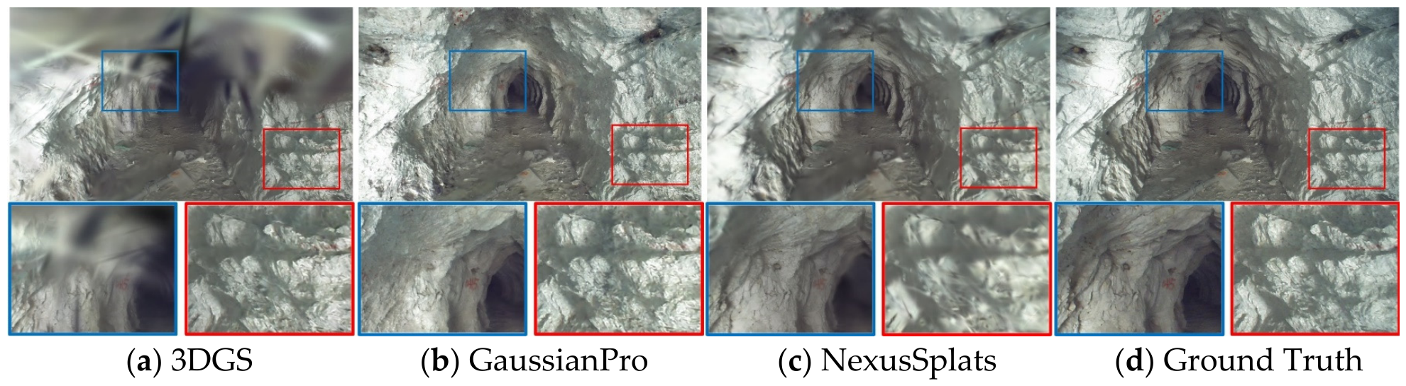
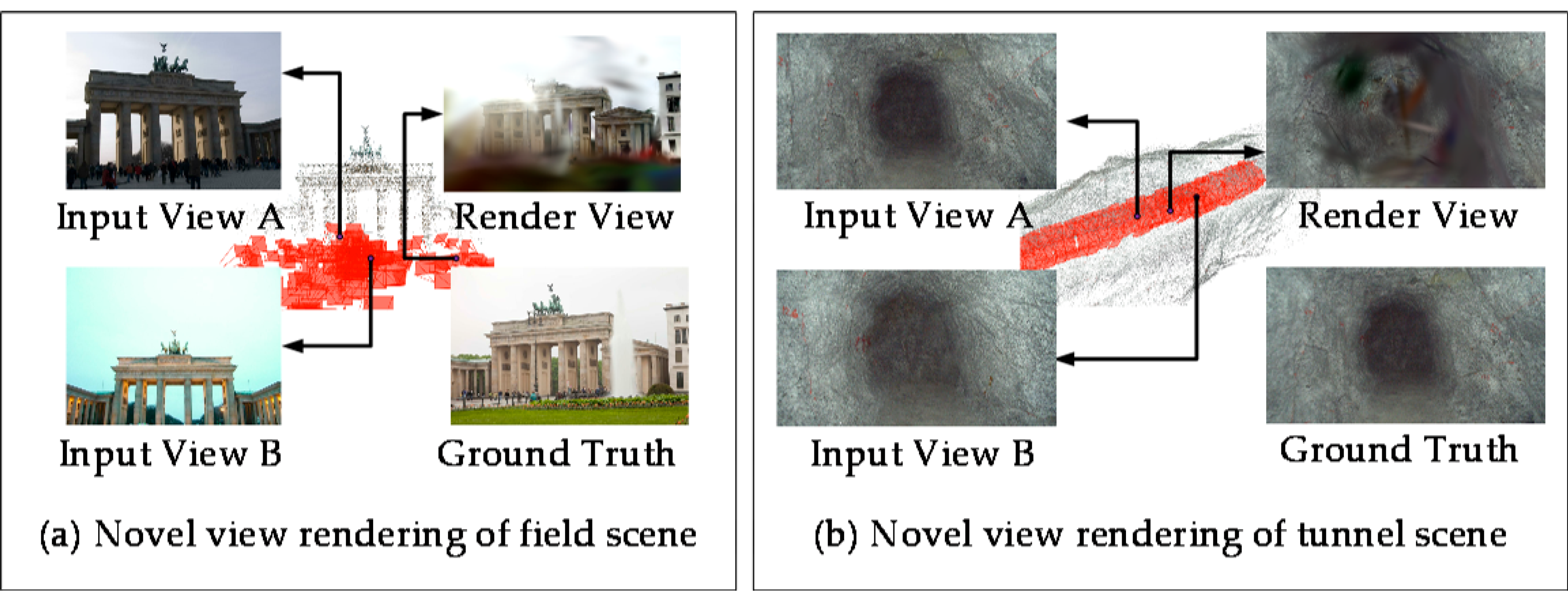
Despite these advances, existing 3DGS methods still rely heavily on multi-view photometric consistency, which becomes fragile under illumination changes [31]. This issue is particularly pronounced in tunnel environments, where natural illumination is largely absent, and image acquisition often depends on localized active lighting mounted on the capture platform. Because such lighting is spatially limited and changes with viewpoint and motion, the same surface may exhibit strong appearance variation across views, creating optimization ambiguities and leading to lighting-induced artifacts in novel views (Figure 1). Related efforts for handling photometric variation have been explored in both radiance field and Gaussian-based methods, including appearance embeddings, exposure-aware modeling, relightable Gaussian representations, and global appearance harmonization strategies [32,33,34,35,36,37,38,39,40,41].

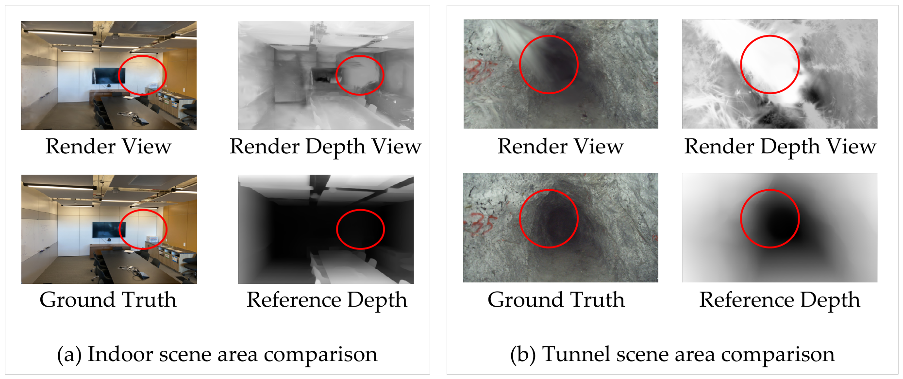
In addition to illumination variation, tunnel reconstruction is further challenged by under-illuminated regions outside the main light coverage. These areas are not necessarily textureless in the physical sense; however, due to insufficient illumination, they often appear weakly textured, low-contrast, and poorly constrained in the captured images. As a result, photometric supervision becomes less reliable, and the spatial optimization of Gaussian primitives can become unstable, producing floating artifacts, inconsistent rendered depth, and spatial distortions even when rendered colors remain visually plausible (Figure 2). Existing studies have introduced depth or structural priors to improve optimization stability in such poorly constrained regions, including voxel-anchored representations, depth-regularized optimization, and depth-guided densification strategies [42,43,44,45].

For scenes affected by both illumination-induced appearance inconsistency and shadow-induced weak visual constraints, previous 3DGS variants based on appearance decoupling [37] or depth regularization [44] can mitigate floating artifacts to some extent. However, as illustrated in Figure 3, they still exhibit varying degrees of texture degradation or residual instability because the two failure modes are mainly handled separately rather than jointly. This observation motivates a unified framework that simultaneously incorporates lighting-adaptive appearance modeling and depth-guided spatial regularization for tunnel-oriented reconstruction.

In practice, these two issues are tightly coupled in Gaussian optimization. Dynamic lighting corrupts the photometric cues used for appearance fitting, while shadowed under-illuminated regions often appear weakly textured and provide insufficient constraints for stable Gaussian placement; together, they amplify floating artifacts and reconstruction instability. This coupled failure pattern is especially pronounced in tunnel scenes captured under localized active illumination.

To address these issues, this paper proposes DLG-GS, a dynamic lighting-aware real-time 3D Gaussian splatting framework designed primarily for tunnel scenes captured under localized active illumination. DLG-GS contains two complementary components. First, a dynamic lighting-adaptive appearance modeling strategy leverages Fourier-encoded spatial descriptors, view-dependent illumination cues, and local multi-granularity attention to disentangle intrinsic appearance from transient lighting effects while preserving high-frequency texture details. Second, a voxel–depth joint constraint introduces monocular depth priors into the optimization of voxel anchors and neural Gaussians, thereby regularizing their spatial distribution, improving rendered-depth consistency, and suppressing floating artifacts in shadow-induced weak-texture regions. By jointly optimizing lighting-adaptive appearance modeling and depth-guided spatial regularization within a unified framework, DLG-GS improves reconstruction stability under dynamic lighting while maintaining real-time rendering performance. Although the framework is developed with tunnel scenes as the primary target, we also evaluate its transferability on several public benchmarks.

The main contributions of this work are summarized as follows:

We propose DLG-GS, a tunnel-oriented real-time 3D Gaussian splatting framework that explicitly addresses the coupled challenges of dynamic-lighting-induced appearance inconsistency and shadow-induced weakly constrained regions during reconstruction.

The framework introduces a dynamic lighting-adaptive appearance modeling strategy that combines Fourier-based spatial encoding, view-dependent illumination descriptors, and local multi-granularity attention to reduce illumination-induced artifacts while preserving fine texture details.

The proposed voxel–depth joint constraint regularizes the spatial distribution of voxel anchors and neural Gaussians using monocular depth priors, improving reconstruction stability and suppressing floating artifacts in shadowed weak-texture regions.

Experiments on a challenging self-collected tunnel dataset show clear improvements over the selected baselines, while additional evaluations on public benchmarks indicate that the proposed method remains competitive beyond the target tunnel setting, all while preserving real-time rendering capability.

2. Materials and Methods

2.1. Problem Analysis and Framework Overview

Three-dimensional reconstruction in tunnel scenes captured under localized active illumination faces two coupled challenges when applying the original 3DGS framework.

• The challenge of appearance inconsistency under dynamic lighting: Because tunnel environments usually lack stable ambient illumination, image acquisition often depends on localized active light sources mounted on the capture platform. As the platform moves, the illumination pattern changes with viewpoint and position, causing the same surface to exhibit noticeable appearance differences across views. This weakens the multi-view photometric consistency assumption of 3DGS and leads to ambiguous appearance fitting, color distortion, and floating artifacts.
• The challenge of shadow-induced weak constraints: Another difficulty arises in under-illuminated shadow regions. These regions are not necessarily textureless in the physical sense, but they often appear weakly textured, low-contrast, and poorly constrained in the captured images. Under such conditions, photometric supervision becomes unreliable, and the spatial optimization of Gaussian primitives tends to become unstable, resulting in irregular Gaussian distributions, rendered-depth inconsistency, and floating artifacts.

To address the above challenges, this paper proposes the DLG-GS framework. Its core idea is to jointly optimize lighting-adaptive appearance modeling and depth-prior-guided spatial regularization within a unified 3DGS framework.

• DLAAM: This module is designed to disentangle intrinsic scene appearance from transient illumination effects. By combining Fourier-encoded spatial descriptors, view-dependent illumination cues, and local multi-granularity attention, it improves appearance consistency under dynamic lighting while preserving local texture details.
• VDJC: This module introduces monocular depth priors to regularize the spatial distribution of voxel anchors and neural Gaussians. It improves rendered-depth consistency and suppresses floating artifacts, especially in shadow-induced weakly constrained regions.

To further couple the two modules, DLAAM provides an appearance-guided weighting signal for VDJC. Specifically, the discrepancy between the illumination-adapted appearance and the original rendered color is used as a heuristic cue to construct an appearance-guided weighting map. Under localized active illumination, regions with a smaller discrepancy are treated as more likely to be under-illuminated and weakly constrained, and are therefore assigned stronger depth-guided spatial regularization in VDJC.

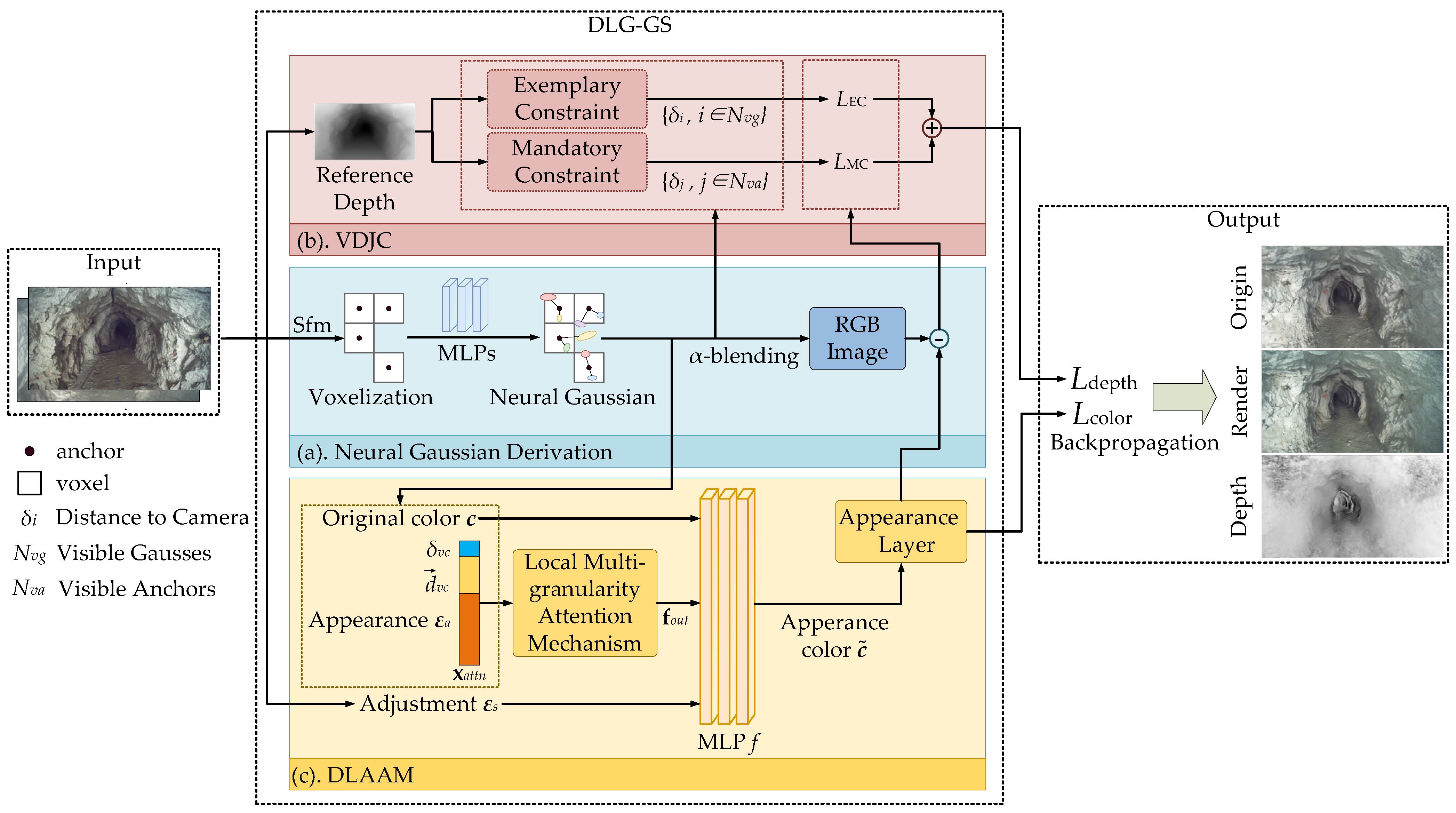
DLG-GS is built upon the voxelized neural Gaussian architecture of Scaffold-GS [30]. The overall pipeline is illustrated in Figure 4. Based on the initial voxel–neural Gaussian representation, VDJC introduces dual depth constraints to stabilize Gaussian optimization in weakly constrained regions (Section 2.2), while DLAAM enhances appearance prediction and provides the appearance-guided weighting signal for adaptive depth regularization (Section 2.3). These two modules are jointly embedded into the optimization process of 3DGS.

2.2. Voxel–Depth Joint Constraint (VDJC)

During training, 3DGS optimization may rely excessively on fitting individual training views, leading to redundant Gaussians and unstable spatial distributions. As discussed in Section 2.1, these problems become more severe in under-illuminated shadow regions, where the captured images often appear weakly textured, low-contrast, and poorly constrained. In such regions, photometric supervision alone is insufficient to provide stable guidance for Gaussian optimization, making floating artifacts and rendered-depth inconsistency more likely to occur. Although the voxel anchors in Scaffold-GS provide an initial spatial prior, the generation and optimization of neural Gaussians still depend mainly on photometric error, which remains unreliable in these weakly constrained areas. Recent methods such as GaussianPro [44] also introduce depth supervision into 3D Gaussian splatting, but they mainly use per-ray depth consistency losses between rendered depth and predicted depth maps. While such strategies can improve optimization stability in some cases, they do not explicitly regularize the joint spatial distribution of voxel anchors and neural Gaussians, nor are they specifically designed for the shadow-induced weak-constraint regions commonly encountered in tunnel scenes under localized active illumination.

To improve optimization stability in weakly constrained regions, we introduce the voxel–depth joint constraint (VDJC) module. VDJC uses monocular depth priors as a spatial regularization signal for voxel anchors and neural Gaussians, with the goal of stabilizing Gaussian optimization and improving rendering quality under weak visual constraints. Specifically, the module regularizes the spatial distribution of neural Gaussians at two levels: an exemplary constraint (EC) at the neural Gaussian level and a mandatory constraint (MC) at the voxel-anchor level. The EC provides fine-grained depth guidance by encouraging the rendered depth of neural Gaussians to remain consistent with the estimated depth map, which helps reduce local depth ambiguity. The MC further imposes anchor-level depth regularization on the voxel representation, encouraging the generated Gaussians to remain spatially consistent with the underlying depth prior and thereby providing a stronger structural constraint on their overall distribution. By combining these two levels of regularization, VDJC helps suppress irregular Gaussian placement, floating artifacts, and rendered-depth inconsistency in shadow-induced weak-texture regions. This voxel–depth joint design is particularly suitable for tunnel scenes under localized active illumination, where local photometric cues are often unreliable and Gaussian optimization benefits from both fine-grained depth guidance and anchor-level spatial regularization.

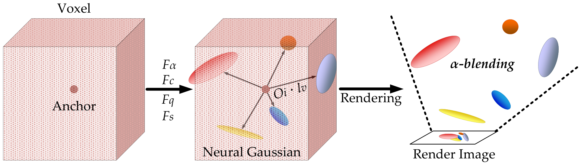
First, we clarify the voxel–neural Gaussian model generated by the Scaffold-GS framework. Simply put, Scaffold-GS uses the points from the initial point cloud as the initial positions $\mathbf{V}\in {\mathbb{R}}^{\tilde{N}\times 3}$ for generating voxels, establishing geometric priors by voxelizing the 3D space. Each voxel $\mathrm{v}\in \mathbf{V}$ is centered with an anchor point $x_v$, equipped with a local feature $f_v\in {\mathbb{R}}^{32}$, a scaling factor $l_v\in {\mathbb{R}}^3$, and k learnable offsets $O_v\in {\mathbb{R}}^{k\times 3}$. Using these attributes of the voxel anchor, the attributes of each neural Gaussian are dynamically predicted based on viewing direction and distance. The specific process is illustrated in Figure 5.

The position of each neural Gaussian is derived by summing the anchor position with the product of its offsets and scaling factor. Other Gaussian attributes—opacity $\alpha$, color $c$, quaternion $q$ (related to covariance), and scaling $s$—are predicted from the anchor feature $f_v$, the relative viewing distance ${\delta }_{vc}$, and the viewing direction ${\overrightarrow{d}}_{vc}$ through corresponding MLPs (denoted as $F_{\alpha }$, $F_c$, $F_q$, and $F_s$). Subsequently, using a differentiable point rendering technique, the 3D Gaussian primitives are projected onto a 2D imaging plane after being sorted by depth. The pixel colors are then computed via α-blending, resulting in a rendered 2D image. The photometric loss $L_1$ and SSIM loss $L_{\mathrm{S}\mathrm{S}\mathrm{I}\mathrm{M}}$ are computed between the rendered image and the Ground Truth (GT) [46]. Based on the gradient magnitude of the neural Gaussians, new anchors are dynamically added and redundant anchors that fail to generate valid Gaussians are removed, thereby improving computational efficiency.

Building upon the voxel–neural Gaussian representation, we introduce depth priors to regularize the spatial distribution of Gaussians. As noted above, voxel anchors not only determine where neural Gaussians are generated but also provide the inputs used to predict their other attributes. For this reason, we do not directly impose large position updates on the anchors. Instead, we regularize the generated neural Gaussians and use this process to indirectly improve their spatial arrangement. As shown in Figure 4b, the VDJC module takes three inputs: monocular depth predictions, voxel-anchor positions, and neural Gaussian positions. We first apply the exemplary constraint (EC) at the neural Gaussian level. Specifically, we fix the scale ($s$) and rotation ($q$) of each Gaussian and optimize only its position ($u$) and opacity ($\alpha$), so that the Gaussian can better match the depth prior through spatial relocation rather than compensating for supervision errors by changing its shape. For monocular depth estimation, we use the pretrained large version of Depth Anything V2 [47] to predict a reference depth map $D_r$ from each training image. Since monocular depth predictions are scale-ambiguous, we use the normalized depth map as a relative structural prior rather than as metric geometric ground truth. Before computing the depth losses, the predicted and rendered depth maps are normalized to a comparable range. Based on the current neural Gaussian positions generated from voxel anchors and their learned offsets, we then render a depth map by computing the camera distance of the visible Gaussians, as defined below:

$$\{\begin{array}{c}{u}_{v,i}=x_v+l_v\cdot O_{v,i}\\ {\delta }_{v,i}={\parallel u_{v,i}-x_c\parallel }_2\end{array},\mathrm{ }i=\mathrm{1,2},\dots ,k$$

(1)

where $u_{v,i}$ denotes the spatial position of the i-th neural Gaussian generated from voxel anchor $v$, $x_v$ denotes the position of the anchor point at the voxel center, $O_{v,i}$ denotes the corresponding offset vector, and $l_v$ denotes the scaling factor associated with that voxel. For the current camera view with optical center $x_c$, the depth value ${\delta }_{v,i}$ is defined as the distance from $u_{v,i}$ to $x_c$.

After obtaining the neural Gaussian positions, we render a depth map by using their camera distances as depth values in the splatting process. Specifically, the rendered depth map $D_{ng}$ is computed by α-blending the depth contributions of the projected neural Gaussians, as defined below:

$$D_{ng}\left(p\right)={\sum }_{i=1}^{N_p}\left({\delta }_i\cdot {\sigma }_i\cdot {\prod }_{j=1}^{i-1}\left(1-{\sigma }_j\right)\right),\mathrm{ }{\sigma }_i={\alpha }_i{G}^{\prime }\left(p\right)$$

(2)

where $p$ denotes a pixel location in the rendered depth map $D_{ng}$, $N_p$ denotes the number of depth-sorted projected Gaussians contributing to pixel $p$, and ${\delta }_i$ denotes the distance from the i-th visible neural Gaussian to the camera center in the current view. The term ${\sigma }_i$ denotes the effective opacity weight of the i-th Gaussian, computed from its learned opacity ${\alpha }_i$ and its projected 2D Gaussian value $G^{\prime }\left(p\right)$. The resulting $D_{ng}$ represents the depth map implied by the current spatial distribution of neural Gaussians and is then compared with the monocular depth prior for optimization.

In parallel with the neural-Gaussian-level regularization, we further introduce the mandatory constraint (MC) at the voxel-anchor level. Instead of using the positions of the generated neural Gaussians, this constraint renders depth by using the corresponding voxel-anchor positions as the depth carriers while keeping the opacity term fixed. In this way, the rendered depth is determined by the anchor locations that underlie Gaussian generation, allowing the depth prior to directly regularize the coarse spatial layout of the anchor representation. The corresponding anchor-level rendered depth map $D_{va}$ is defined in Equation (3).

$$D_{va}(p)={\sum }_{i=1}^{N_p}({\parallel x\left(u_i\right)-x_c\parallel }_2\cdot {\sigma }_i^{\prime }\cdot {\prod }_{j=1}^{i-1}(1-{\sigma }_j^{\prime })), {\sigma }_i^{\prime }=\tau G^{\prime }\left(p\right)$$

(3)

where $x\left(u_i\right)$ denotes the position of the voxel anchor that generates the neural Gaussian $u_i$, $\tau$ denotes the fixed opacity value used in this constraint, and ${\parallel x\left(u_i\right)-x_c\parallel }_2$ indicates the replacement of the distance from the neural Gaussian to camera $x_c$ with the distance from the anchor point to camera $x_c$. The remaining variables follow the same definitions as in Equation (2). Compared with the neural-Gaussian-level constraint, this anchor-level depth rendering provides a stronger structural regularization signal for the underlying voxel representation, which helps stabilize the overall spatial distribution of the generated Gaussians in weakly constrained regions.

Finally, we combine the two rendered depth maps described above to regularize the spatial distribution of Gaussians under the monocular depth prior. Specifically, the neural-Gaussian-level depth map $D_{ng}$ and the anchor-level depth map $D_{va}$ are both compared with the reference depth map $D_r$ using pixel-wise depth differences. To make the regularization adaptive to lighting-induced uncertainty, we further introduce a pixel-wise weighting term $\widehat{\omega }\left(p\right)$, which modulates the strength of the depth loss at each pixel. The detailed construction of this weighting term is introduced later in Section 2.3. The two depth loss components are defined as:

$$\{\begin{array}{c}{L}_{\mathrm{E}\mathrm{C}}={\displaystyle \frac{1}{W\times H}}{\sum }_{i=1}^W{\sum }_{j=1}^H\left(\widehat{\omega }\left(p\right)\cdot \left|D_{ng}\left(i,j\right)-D_r\left(i,j\right)\right|\right)\\ L_{\mathrm{M}\mathrm{C}}={\displaystyle \frac{1}{W\times H}}{\sum }_{i=1}^W{\sum }_{j=1}^H\left(\widehat{\omega }\left(p\right)\cdot \left|D_{va}\left(i,j\right)-D_r\left(i,j\right)\right|\right)\end{array}$$

(4)

where $W\times H$ denotes the pixel dimensions of the image. The weighting term $\widehat{\omega }\left(p\right)$ is used to adaptively strengthen depth regularization in regions that are more likely to be weakly constrained. The two loss components are combined to form the overall constraint loss function $L_{\mathrm{d}\mathrm{e}\mathrm{p}\mathrm{t}\mathrm{h}}$ for regulating the neural Gaussian distribution:

$$L_{\mathrm{d}\mathrm{e}\mathrm{p}\mathrm{t}\mathrm{h}}={\lambda }_{\mathrm{E}\mathrm{C}}{L}_{\mathrm{E}\mathrm{C}}+{\lambda }_{\mathrm{M}\mathrm{C}}{L}_{\mathrm{M}\mathrm{C}}$$

(5)

where ${\lambda }_{\mathrm{E}\mathrm{C}}$ and ${\lambda }_{\mathrm{M}\mathrm{C}}$ are balance weights for the neural-Gaussian-level and anchor-level constraints, respectively. This loss is incorporated into the overall 3DGS optimization and jointly updates the generated neural Gaussians and the underlying voxel-anchor representation during backpropagation. By combining fine-grained depth-guided regularization with anchor-level spatial regularization, VDJC helps suppress irregular Gaussian placement, floating artifacts, and local instability in weakly constrained regions, thereby improving the spatial stability of the learned representation under rendering-oriented optimization.

2.3. Dynamic Lighting-Adaptive Appearance Modeling (DLAAM)

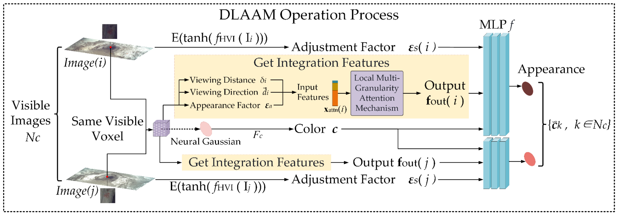
Dynamic lighting disrupts multi-view appearance consistency and is a major source of reconstruction artifacts in tunnel scenes. Existing appearance modeling or decoupling methods (e.g., NexusSplats [37]) can alleviate part of this problem, but they may still over-smooth local details under strong illumination variation. To address this issue, we introduce the dynamic lighting-aware appearance modeling (DLAAM) module, as illustrated in Figure 6. DLAAM aims to separate transient illumination effects from more stable scene appearance while preserving fine-grained local structures during optimization [48]. This design is particularly motivated by two characteristics of tunnel imaging:

• Spatially localized illumination patterns caused by active moving light sources;
• Shadow-affected regions that appear weakly textured and poorly constrained in the captured images.

To model these properties, DLAAM combines Fourier-based spatial encoding, an illumination-sensitive latent representation in the HVI space, and a local multi-granularity attention mechanism.

The combination of Fourier encoding, HVI-based illumination features, and local attention is well-suited to the imaging characteristics of tunnel scenes. Fourier encoding enriches the spatial representation with multi-frequency components, which helps describe localized appearance variations under changing active illumination. The HVI-based representation provides an illumination-sensitive view descriptor extracted from the input image, enabling the model to capture view-dependent lighting changes more effectively. Based on these cues, the local multi-granularity attention mechanism further aggregates nearby contextual features, helping suppress transient illumination disturbance while preserving local structural details. This design is motivated by the tunnel setting, where the scene layout is highly repetitive and elongated, whereas the illumination pattern can vary noticeably along the acquisition trajectory.

The workflow of DLAAM is illustrated in Figure 4c and consists of three stages. Factor encoding: an appearance factor ${\mathit{\epsilon }}_a$ is extracted from the voxel representation, and an image-dependent adjustment factor ${\mathit{\epsilon }}_s$ is introduced to characterize view-specific illumination variation. Context fusion: these factors are integrated with local spatial context through a local multi-granularity attention mechanism, producing a refined feature representation ${\mathbf{f}}_{out}$. Appearance decoupling: based on the refined feature ${\mathbf{f}}_{out}$, a lightweight MLP $f$ predicts color adjustment parameters for each neural Gaussian, yielding an illumination-decoupled appearance color $\tilde{\mathit{c}}$ for rendering.

First, DLAAM constructs feature representations from the voxel anchors, the input image, and the original Gaussian color prediction. Specifically, its inputs include: (1) a voxel appearance factor ${\mathit{\epsilon }}_a$ derived from the anchor coordinates, (2) an image-dependent adjustment factor ${\mathit{\epsilon }}_s$ extracted from the current training view, and (3) the original color $\mathit{c}$ predicted for each neural Gaussian. For the voxel appearance factor, we apply a Fourier-based coordinate encoding to the spatially distributed voxel anchors. By using multi-frequency mapping together with phase shifting, the raw 3D coordinates of each anchor are transformed into a feature representation with richer spectral content:

$${\mathit{\epsilon }}_a^{\left(j\right)}=\mathsf{\Phi }\left(x_v^{\left(j\right)}\right)=\mathrm{concat}\left(\mathrm{s}\mathrm{i}\mathrm{n}(2\pi {\mathit{\omega }}_{\kappa }{x}_v^{\left(j\right)}+{\mathit{\varphi }}_{\kappa }),\mathrm{c}\mathrm{o}\mathrm{s}(2\pi {\mathit{\omega }}_{\kappa }{x}_v^{\left(j\right)}+{\mathit{\varphi }}_{\kappa })\right)$$

(6)

where ${\mathit{\epsilon }}_a^{\left(j\right)}$ denotes the appearance factor for the j-th anchor (each anchor is learned independently), $\mathsf{\Phi }\left(·\right)$ represents its Fourier-based feature encoding. $x_v^{\left(j\right)}$ is the center coordinate of the j-th voxel anchor. $\mathrm{concat}\left(·\right)$ denotes concatenation along the feature dimension, ${\mathit{\omega }}_{\kappa }$ denotes the exponentially increasing frequency basis vector ($\kappa =1,\dots ,K$), and ${\mathit{\varphi }}_{\kappa }$ denotes the alternating phase shift vector.

For each training view, we derive an image-dependent adjustment factor ${\mathit{\epsilon }}_s$ from the HVI representation [49] of the input image to characterize view-specific illumination variation:

$${\mathit{\epsilon }}_s^{\left(t\right)}=\mathrm{t}\mathrm{a}\mathrm{n}\mathrm{h}\left(f_{\mathrm{H}\mathrm{V}\mathrm{I}}\left({\mathbf{I}}_t\right)\right)$$

(7)

where ${\mathbf{I}}_t$ denotes the t-th training image, $f_{\mathrm{H}\mathrm{V}\mathrm{I}}$ denotes the HVI-based feature extractor, $\mathrm{t}\mathrm{a}\mathrm{n}\mathrm{h}\left(·\right)$ denotes the hyperbolic tangent function used to stabilize the feature response, and ${\mathit{\epsilon }}_s^{\left(t\right)}$ denotes the resulting adjustment factor for the current view. This factor serves as an illumination-sensitive descriptor that is later fused with the voxel appearance factor for appearance modeling.

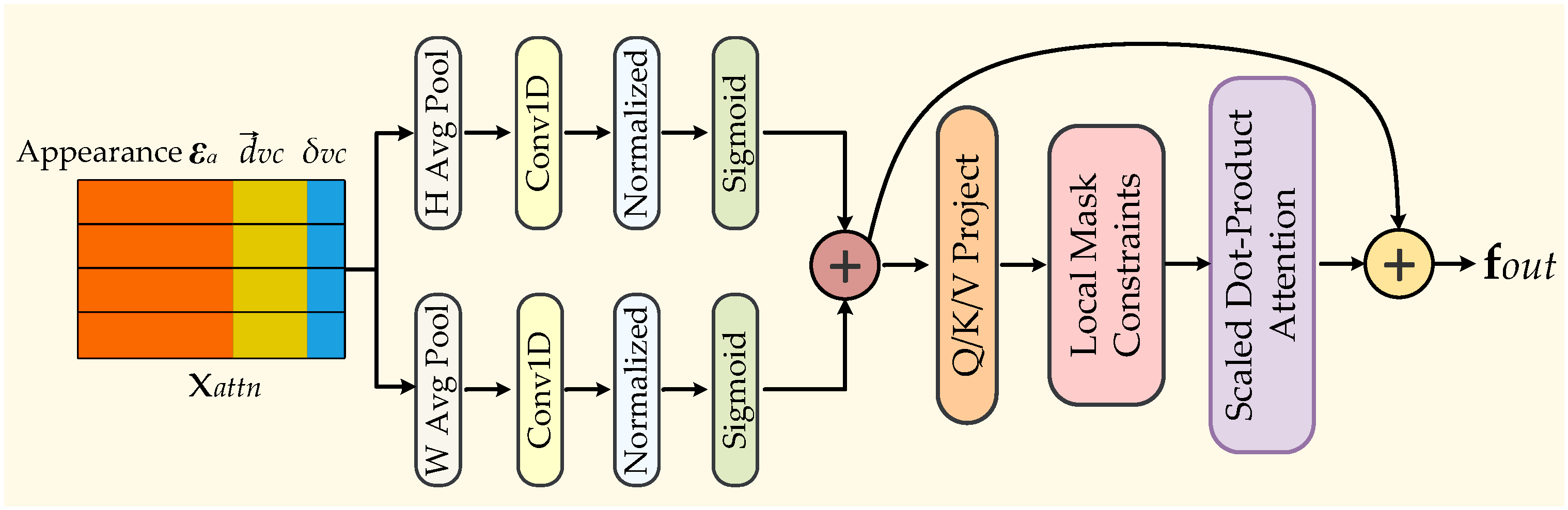
Subsequently, a local multi-granularity attention mechanism is introduced to adaptively fuse the voxel appearance factor with spatial contextual information, so as to refine local appearance features under varying illumination. As illustrated in Figure 7, the voxel appearance factor (${\mathit{\epsilon }}_a$) and positional information (${\delta }_{vc}$ and ${\overrightarrow{d}}_{vc}$) are concatenated to form the input feature ${\mathbf{x}}_{attn}$, which is then fed into the attention module to produce the refined feature ${\mathbf{f}}_{out}$.

During this process, the input feature ${\mathbf{x}}_{attn}={\mathit{\epsilon }}_a^{\left(v\right)}\oplus {\overrightarrow{d}}_{vc}\oplus {\delta }_{vc}$ first undergoes average pooling separately along the vertical (height) and horizontal (width) directions to capture directional contextual statistics. The pooled features are then passed through a 1D convolution followed by a Sigmoid activation, yielding attention weights for feature refinement. These weights (the anchored dimension attention ${\mathbf{z}}_h$ and the feature dimension input features ${\mathbf{z}}_w$) are broadcast and multiplied with the input feature to obtain the granularity-refined feature ${\mathbf{f}}_{\mathrm{g}\mathrm{r}\mathrm{a}}$, as defined in Equation (8).

$${\mathbf{f}}_{\mathrm{g}\mathrm{r}\mathrm{a}}={\mathbf{x}}_{attn}\odot {\mathbf{z}}_h\odot {\mathbf{z}}_w,\{\begin{array}{c}{\mathbf{z}}_h=\mathrm{s}\mathrm{i}\mathrm{g}\left(\mathrm{C}\mathrm{o}\mathrm{n}\mathrm{v}1\mathrm{D}\left(\mathrm{A}\mathrm{v}\mathrm{g}\mathrm{P}\mathrm{o}\mathrm{o}{\mathrm{l}}_h\left({\mathbf{x}}_{attn}\right)\right)\right)\\ {\mathbf{z}}_w=\mathrm{s}\mathrm{i}\mathrm{g}\left(\mathrm{C}\mathrm{o}\mathrm{n}\mathrm{v}1\mathrm{D}\left(\mathrm{A}\mathrm{v}\mathrm{g}\mathrm{P}\mathrm{o}\mathrm{o}{\mathrm{l}}_w\left({\mathbf{x}}_{attn}\right)\right)\right)\end{array}$$

(8)

where $\mathrm{s}\mathrm{i}\mathrm{g}\left(·\right)$ denotes the Sigmoid activation function, and $\odot$ denotes element-wise multiplication with broadcasting.

Subsequently, a local self-attention mechanism is applied to the granularity-refined feature ${\mathbf{f}}_{\mathrm{g}\mathrm{r}\mathrm{a}}$ to further model local dependencies and enhance structural context. Specifically, ${\mathbf{f}}_{\mathrm{g}\mathrm{r}\mathrm{a}}$ is projected into the query, key, and value subspaces, denoted by Query (Q), Key (K), and Value (V), through learnable linear transformations:

$$\mathbf{Q}={\mathbf{W}}_q{\mathbf{f}}_{\mathrm{g}\mathrm{r}\mathrm{a}},\mathrm{ }\mathbf{K}={\mathbf{W}}_k{\mathbf{f}}_{\mathrm{g}\mathrm{r}\mathrm{a}},\mathbf{ }\mathbf{V}={\mathbf{W}}_v{\mathbf{f}}_{\mathrm{g}\mathrm{r}\mathrm{a}}$$

(9)

where ${\mathbf{W}}_q,{\mathbf{W}}_k,{\mathbf{W}}_v\in {\mathbb{R}}^{d\times d_k}$ are learnable projection matrices that map the input into the semantic spaces of Q, K, and V, respectively, $d$ denotes the input feature dimension, and $d_k$ denotes the dimensionality of the key vectors.

To reduce computational cost while preserving local structural interactions, we introduce a local attention mask ${\mathbf{M}}_{local}$, which restricts each anchor to attend only to its spatially neighboring anchors. The pairwise feature correlations are then computed using masked scaled dot-product attention:

$${\mathbf{M}}_{local}[i,j]=\{\begin{array}{c}0, \mathrm{if} {\parallel {\mathrm{pos}}_i-{\mathrm{pos}}_j\parallel }_2\le r \\ -\infty , else \end{array}$$

(10)

where ${\mathbf{M}}_{local}$ denotes the local attention mask, $r$ denotes the predefined neighborhood radius, and ${\mathrm{pos}}_i$ and ${\mathrm{pos}}_j$ denote the spatial positions of the i-th and j-th anchors, respectively. In this way, attention is confined to local neighborhoods, which helps improve computational efficiency while preserving local structural dependencies.

The resulting attention weights are used to aggregate contextual information and produce the refined feature ${\mathbf{f}}_{out}$:

$${\mathbf{f}}_{out}=\mathrm{Attention}(\mathbf{Q},\mathbf{K},\mathbf{V})=\mathrm{S}\mathrm{o}\mathrm{f}\mathrm{t}\mathrm{m}\mathrm{a}\mathrm{x}({\displaystyle \frac{\mathbf{Q}{\mathbf{K}}^{\mathrm{T}}}{\sqrt{d_k}}}+{\mathbf{M}}_{local})\mathbf{V}$$

(11)

The refined feature ${\mathbf{f}}_{out}$, which integrates multi-granularity contextual cues and local structural information, is then fed into the appearance-decoupling MLP $f$ to predict the appearance-related color adjustment parameters.

Finally, a lightweight appearance-decoupling MLP $f$ is used to dynamically predict the color adjustment parameters for each neural Gaussian. Specifically, the attention feature ${\mathbf{f}}_{out}^{\left(j\right)}$, the image adjustment factor ${\mathit{\epsilon }}_s^{\left(t\right)}$, and the original color ${\mathit{c}}_i$ predicted by the baseline Scaffold-GS branch are concatenated and fed into $f$, which outputs an appearance-related reference color component and a corresponding fusion weight. These outputs are then used to generate the view-adaptive appearance color of the neural Gaussian. The formulation is given in Equation (12).

$${\mathsf{\alpha }}_i,{\mathsf{\beta }}_i=f({\mathit{c}}_i,{\mathit{\epsilon }}_s^{\left(t\right)},{\mathbf{f}}_{out}^{\left(j\right)})$$

(12)

where ${\mathit{c}}_i$ denotes the original color of the i-th neural Gaussian generated from the j-th anchor in the baseline Scaffold-GS branch, ${\mathit{\epsilon }}_s^{\left(t\right)}$ denotes the image adjustment factor of the current view ${\mathbf{I}}_t$, and ${\mathbf{f}}_{out}^{\left(j\right)}$ denotes the refined feature produced by the attention module for the j-th anchor. The MLP $f$ outputs a reference color component ${\mathsf{\alpha }}_i$ and a fusion weight ${\mathsf{\beta }}_i$, which are used to compute the final view-adaptive appearance color.

The structure of the appearance-decoupling MLP $f$ is illustrated in Figure 8. The network consists of three fully connected layers with ReLU activations between successive layers. A Sigmoid activation is applied to the final layer to constrain the output to [0, 1], yielding the color-related adjustment parameters. Owing to its lightweight design, this module introduces only limited additional computational overhead during training and inference.

The output of the MLP is combined with the original color through a weighted sum to obtain the view-adaptive appearance color of each neural Gaussian:

$${\tilde{\mathit{c}}}_i={\mathsf{\beta }}_i{\mathit{c}}_i+\left(1-{\mathsf{\beta }}_i\right){\mathsf{\alpha }}_i$$

(13)

The resulting appearance color ${\tilde{\mathit{c}}}_i$ then replaces the original color ${\mathit{c}}_i$ in the rendering process, enabling the model to better adapt to illumination-induced appearance changes across views.

Using the appearance-adaptive colors of the neural Gaussians generated from visible anchors within the current camera frustum, the appearance rendering image ${\mathbf{I}}_a$ is obtained via α-blending:

$${\mathbf{I}}_a\left(p\right)={\sum }_{i=1}^{N_p}\left({\tilde{\mathit{c}}}_i\cdot {\sigma }_i\cdot {\prod }_{j=1}^{i-1}\left(1-{\sigma }_j\right)\right)$$

(14)

where $p$ denotes a pixel location in the appearance rendering image ${\mathbf{I}}_a$, $N_p$ denotes the number of depth-sorted 2D Gaussians contributing to pixel $p$, and ${\sigma }_i$ denotes the effective opacity weight of the i-th Gaussian, computed from its learned opacity (${\alpha }_i$) and projected 2D Gaussian ($G^{\prime }\left(p\right)$) response.

Similarly, the original rendering image ${\mathbf{I}}_r$ is obtained by rendering the same neural Gaussians with their original colors. Based on the discrepancy between ${\mathbf{I}}_a$ and ${\mathbf{I}}_r$, we further construct an appearance-guided weighting map as follows:

$$\widehat{\omega }\left(p\right)=1-\mathrm{c}\mathrm{l}\mathrm{i}\mathrm{p}\left(\parallel {\mathbf{I}}_a\left(p\right)-{\mathbf{I}}_r\left(p\right)\parallel ,\mathrm{0,1}\right)$$

(15)

where larger values correspond to smaller appearance discrepancies. In our setting, such pixels are more likely to belong to shadow-induced weak-texture regions, where appearance adaptation remains limited and photometric supervision is still insufficient. Therefore, in the VDJC optimization, larger weights are assigned to these pixels to strengthen depth regularization, thereby establishing an explicit coupling between appearance adaptation and geometry stabilization.

For appearance supervision, a photometric reconstruction loss ($L_1$) is imposed on ${\mathbf{I}}_a$, while a structural similarity loss ($L_{\mathrm{S}\mathrm{S}\mathrm{I}\mathrm{M}}$) is imposed on ${\mathbf{I}}_r$. In this way, ${\mathbf{I}}_a$ mainly accounts for view-dependent illumination adaptation, whereas ${\mathbf{I}}_r$ helps preserve structural consistency in the baseline rendering branch. The resulting color-related loss is defined as:

$$L_{\mathrm{c}\mathrm{o}\mathrm{l}\mathrm{o}\mathrm{r}}=(1-{\lambda }_{\mathrm{S}\mathrm{S}\mathrm{I}\mathrm{M}})L_1({\mathbf{I}}_a,{\mathbf{I}}_t)+{\lambda }_{\mathrm{S}\mathrm{S}\mathrm{I}\mathrm{M}}{L}_{\mathrm{S}\mathrm{S}\mathrm{I}\mathrm{M}}\left({\mathbf{I}}_r,{\mathbf{I}}_t\right)$$

(16)

2.4. Joint Optimization Objective

To jointly optimize appearance adaptation and geometry stabilization, the proposed framework is trained with a unified objective consisting of four components: a color reconstruction loss $L_{\mathrm{c}\mathrm{o}\mathrm{l}\mathrm{o}\mathrm{r}}$, an appearance-guided depth regularization loss $L_{\mathrm{d}\mathrm{e}\mathrm{p}\mathrm{t}\mathrm{h}}$, a volume regularization term $L_{\mathrm{v}\mathrm{o}\mathrm{l}}$, and a random dropout regularization term $L_{\mathrm{A}\mathrm{R}\mathrm{D}\mathrm{R}}$. Among them, $L_{\mathrm{c}\mathrm{o}\mathrm{l}\mathrm{o}\mathrm{r}}$ encourages illumination-adaptive appearance modeling, $L_{\mathrm{d}\mathrm{e}\mathrm{p}\mathrm{t}\mathrm{h}}$ regularizes the spatial distribution of neural Gaussians in weakly constrained regions, $L_{\mathrm{v}\mathrm{o}\mathrm{l}}$ suppresses excessive Gaussian expansion, and $L_{\mathrm{A}\mathrm{R}\mathrm{D}\mathrm{R}}$ improves robustness by preventing the model from over-relying on a small subset of Gaussians.

To discourage overly large Gaussian supports and reduce redundant spatial overlap, we adopt a volume regularization term:

$$L_{\mathrm{vol}}={\sum }_{i=1}^{N_{ng}}\mathrm{P}\mathrm{r}\mathrm{o}\mathrm{d}\left(s_i\right)$$

(17)

where $N_{ng}$ denotes the number of neural Gaussians in the scene, $\mathrm{P}\mathrm{r}\mathrm{o}\mathrm{d}(·)$ calculates the product of vector components, and $s_i$ represents the scale parameters of each neural Gaussian.

To further improve robustness during training, we introduce appearance random dropout regularization [50]. Specifically, each neural Gaussian is assigned a binary activation mask $m_i$, sampled as:

$$\{\begin{array}{c}{m}_i =\left[\mathrm{Uniform}\left(\mathrm{0,1}\right)>\gamma \right], i=\mathrm{1,2},\dots N_{ng} \\ {\widehat{\mathbf{I}}}_a\left(p\right)={\sum }_{i=1}^N\left({\tilde{c}}_i·m_i·{\sigma }_i·{\prod }_{j=1}^{i-1}(1-m_j·{\sigma }_j)\right) \end{array}$$

(18)

where $\gamma$ is the dropout probability and $\left[·\right]$ denotes the Iverson bracket. Based on the sampled masks, a dropout sub-model is formed by temporarily disabling a subset of neural Gaussians during training. Let ${\widehat{\mathbf{I}}}_a$ denote the appearance rendering produced by this dropout sub-model. The random dropout regularization loss is then defined as:

$$L_{\mathrm{A}\mathrm{R}\mathrm{D}\mathrm{R}}=(1-{\lambda }_{\mathrm{S}\mathrm{S}\mathrm{I}\mathrm{M}})L_1({\widehat{\mathbf{I}}}_a,{\mathbf{I}}_a)+{\lambda }_{\mathrm{S}\mathrm{S}\mathrm{I}\mathrm{M}}{L}_{\mathrm{S}\mathrm{S}\mathrm{I}\mathrm{M}}\left({\widehat{\mathbf{I}}}_a,{\mathbf{I}}_a\right)$$

(19)

which encourages the sub-model to remain consistent with the full appearance rendering. In this way, the representation capacity is distributed more evenly across neural Gaussians, reducing overfitting to a few dominant primitives and improving rendering stability under incomplete local support. During inference, all neural Gaussians remain active.

Finally, the overall training objective is formulated as:

$$L=L_{\mathrm{c}\mathrm{o}\mathrm{l}\mathrm{o}\mathrm{r}}+L_{\mathrm{d}\mathrm{e}\mathrm{p}\mathrm{t}\mathrm{h}}+{\lambda }_{\mathrm{v}\mathrm{o}\mathrm{l}}{L}_{\mathrm{v}\mathrm{o}\mathrm{l}}+{\lambda }_{\mathrm{A}\mathrm{R}\mathrm{D}\mathrm{R}}{L}_{\mathrm{A}\mathrm{R}\mathrm{D}\mathrm{R}}$$

(20)

where $L_{\mathrm{c}\mathrm{o}\mathrm{l}\mathrm{o}\mathrm{r}}$ is the color-related loss defined in Equation (16), and $L_{\mathrm{d}\mathrm{e}\mathrm{p}\mathrm{t}\mathrm{h}}$ denotes the appearance-guided weighted depth loss used in VDJC.

Through this unified objective, the appearance branch provides an adaptive weighting cue for geometry regularization, while the spatial regularization branch stabilizes Gaussian placement in under-constrained regions, thereby enabling coupled optimization of appearance and geometry.

3. Results

To evaluate the performance of DLG-GS, we conducted experiments on a self-collected tunnel dataset and several selected public benchmark scenes. The tunnel dataset is designed to reflect the tunnel-oriented setting considered in this work, featuring localized active illumination, shadow-induced weak-texture regions, and complex rock-surface appearances. In addition, representative scenes from the Tanks and Temples dataset [51], the LLFF dataset [52], and the Photo Tourism dataset [53] are included to examine the transferability of the proposed method beyond the tunnel setting. Quantitative comparisons are reported using PSNR, SSIM, and LPIPS, and the evaluation includes the original 3DGS, the baseline Scaffold-GS, and several recent 3DGS-based comparison methods, including NexusSplats. Finally, ablation experiments are conducted to analyze the individual contributions of DLAAM and VDJC.

3.1. Tunnel Data Collection

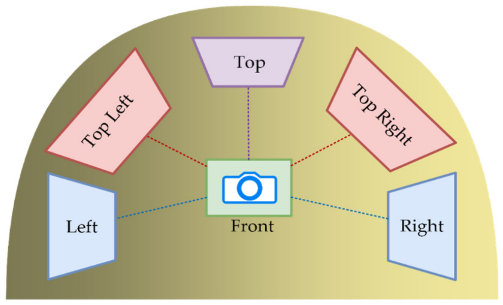
The tunnel dataset used in this study was collected in an enclosed tunnel segment approximately 100–200 m in length, where no stable natural illumination was available during acquisition. As shown in Figure 9, data were captured using a rigid multi-camera platform equipped with six monocular RGB pinhole cameras (1920 × 1080 resolution, 8-bit sRGB). The cameras were arranged to cover the main tunnel surfaces from complementary viewpoints, including the forward direction, the two sidewalls, the vault, and the sidewall–vault transition regions. To ensure consistent imaging geometry, all cameras were rigidly mounted with fixed optical axes throughout data collection.

The imaging parameters were kept unchanged across the acquisition process, including a focal length of 23 mm, an aperture of f/4, an exposure time of 1/60 s, and an ISO sensitivity of 800. Since the tunnel interior lacked stable natural light, a constant-current LED array was mounted at the front of the platform as the primary active illumination source. The LED array had a color temperature of approximately 5000 ± 100 K and produced a spatially varying illumination pattern that attenuated with distance, thereby creating localized bright regions, shadow transitions, and under-illuminated areas in the captured images.

During acquisition, the platform moved incrementally along the tunnel axis, and all six cameras were triggered synchronously at intervals of approximately 50 cm. This setup allowed the collected image sequences to cover the tunnel surfaces from multiple overlapping viewpoints while preserving the dynamic lighting characteristics induced by the moving illumination source.

3.2. Dataset Composition and Implementation Details

For the tunnel-oriented evaluation, we used three representative scenes from the self-collected tunnel dataset, denoted as Tunnel_1, Tunnel_2, and Tunnel_3. Tunnel_1 contains a complete cross-section with the tunnel face, while Tunnel_2 and Tunnel_3 correspond to two longitudinal tunnel sections captured away from the face region under different illumination conditions. These scenes exhibit distinct appearance characteristics, including shadow-dominated weak-texture regions, localized bright areas, and varying rock-surface textures. Camera poses and sparse point clouds are recovered using COLMAP [54], which provides the initialization required for subsequent 3DGS-based optimization. For within-sequence novel-view evaluation, 12.5% of the images are held out as the test set using temporal stratified sampling, with every eighth frame selected for testing.

To provide additional evidence on the behavior of the proposed method beyond the tunnel setting, we further evaluate it on selected scenes from three public benchmarks: Tanks and Temples, LLFF, and Photo Tourism. Tanks and Temples is used to examine performance on general bounded real scenes, LLFF is included to test forward-facing scenes with limited viewpoint variation, and Photo Tourism is used to assess performance under larger appearance variations, illumination differences, and occlusions. Since only selected scenes from these datasets are used, the corresponding results are intended to complement the tunnel-oriented evaluation rather than to establish broad scene-level generalization.

All experiments are conducted on a single NVIDIA RTX 3090 GPU with 24 GB of memory. Each scene is trained for 30,000 iterations. Unless otherwise stated, the implementation inherits the main configuration of Scaffold-GS [30]. The number of neural Gaussians generated per voxel is set to $k$ = 10, the feature dimension is set to $d$ = 28, and the Fourier frequency level is set to $K$ = 4. For the VDJC module, the fixed opacity used in the anchor-level strong depth constraint is set to $\tau$ = 0.95. The loss weights are set to ${\lambda }_{\mathrm{S}\mathrm{S}\mathrm{I}\mathrm{M}}$ = 0.2, ${\lambda }_{\mathrm{v}\mathrm{o}\mathrm{l}}$ = 0.001, ${\lambda }_{\mathrm{E}\mathrm{C}}$ = ${\lambda }_{\mathrm{M}\mathrm{C}}$ = 0.01, and ${\lambda }_{\mathrm{A}\mathrm{R}\mathrm{D}\mathrm{R}}$ = 0.1.

3.3. Baseline

We compared the proposed method with several representative baselines from different perspectives. The original 3DGS and Scaffold-GS [30] are included as foundational references. NexusSplats [37] is used as a particularly relevant comparison because it is also built on a voxel-based representation and introduces appearance-aware modeling for unconstrained image collections. We further included NeRF-W [34] and WildGaussians [41] as appearance-related baselines. To examine the effect of depth-guided regularization in weakly constrained regions, we used GaussianPro as a comparison [44]. In addition, we included 3D Student Splatting and Scooping (SSS) [23], which adopts a non-monotonic mixed representation based on Student’s t-distributions and positive/negative density components to improve expressive capacity and parameter efficiency; 2D Gaussian splatting (2DGS) [22], which uses surface-oriented Gaussian primitives to improve geometric consistency while maintaining efficient rendering; and Mip-Splatting [29], which introduces filtering strategies to reduce aliasing and improve detail stability across views.

To improve the fairness of comparison, all baselines are reproduced using their public implementations whenever available. For each method, we follow the authors’ recommended or default settings as closely as possible. At the same time, the train/test split, input image resolution, and training iteration budget are kept consistent whenever these factors can be unified across methods. Importantly, within each method, the same method-specific hyperparameter configuration is used across different scenes, and no scene-by-scene retuning is performed unless required by the official implementation. This setting is intended to reduce performance variations caused by manual scene-specific adjustment and to make the comparison protocol more consistent across tunnel and non-tunnel scenes.

Quantitative evaluation is reported using PSNR, SSIM, and LPIPS, which measure pixel-level fidelity, structural similarity, and perceptual similarity, respectively. In addition, qualitative comparisons on held-out novel views are provided to examine texture continuity, artifact suppression, and visual consistency under dynamic lighting and shadow-induced weak-texture conditions.

3.4. Analysis of Experimental Results

3.4.1. Tunnel Dataset

Table 1. Quantitative results of different methods on the tunnel test dataset. (The symbol ↓ indicates that lower values in that column represent better quality, while ↑ indicates that higher values represent better quality. Best results per column are bolded; second-best are underlined).

Methods	GPU h/FPS	Tunnel_1			Tunnel_2			Tunnel_3
		PSNR ↑	SSIM ↑	LPIPS ↓	PSNR ↑	SSIM ↑	LPIPS ↓	PSNR ↑	SSIM ↑	LPIPS ↓
NeRF-W	9.15/<1	19.4372	0.6480	0.5256	19.8636	0.7034	0.4957	19.3977	0.6633	0.5353
3DGS	0.53/148	21.5072	0.7449	0.4370	20.7701	0.7890	0.4642	18.2952	0.6568	0.5542
GaussianPro	0.63/120	23.4453	0.7060	0.4107	22.5089	0.7412	0.4226	19.7672	0.6084	0.4696
Scaffold-GS	0.41/160	26.0471	0.7827	0.3934	26.1402	0.8173	0.4117	23.4969	0.7224	0.4538
2DGS	0.56/93	22.1873	0.7453	0.4774	20.0589	0.7612	0.5300	19.2337	0.6658	0.5539
Mip-Splatting	0.63/91	18.7557	0.7192	0.4999	18.1065	0.7498	0.5393	16.0621	0.6534	0.5854
SSS	1.64/30	20.1280	0.6702	0.5283	17.3556	0.6365	0.5966	16.0010	0.6322	0.5551
WildGaussians	4.21/26	25.7487	0.7508	0.6074	26.2512	0.7979	0.6209	23.9182	0.6967	0.6990
NexusSplats	0.93/48	26.3193	0.7481	0.5488	26.3067	0.8118	0.5677	23.3792	0.7117	0.6171
Ours	1.12/52	26.8275	0.7895	0.3899	27.4617	0.8259	0.4059	24.5368	0.7333	0.4561

reports the quantitative results on the three tunnel test scenes. On this tunnel-oriented evaluation, the proposed method achieves the highest PSNR in all three scenes, reaching 26.83 dB, 27.46 dB, and 24.54 dB on Tunnel_1, Tunnel_2, and Tunnel_3, respectively. Compared with Scaffold-GS, the PSNR gains are 0.78 dB, 1.32 dB, and 1.04 dB, respectively, while the improvements over the original 3DGS are larger in all three cases. These results indicate that the proposed appearance adaptation and depth-guided spatial regularization are beneficial under the localized active illumination and shadow-induced weak-texture conditions present in the tunnel dataset.

For SSIM, our method also obtains the highest values across the three scenes, suggesting more stable image-level structural consistency on the held-out views. For LPIPS, the proposed method achieves the best result on Tunnel_1 and Tunnel_2, and the second-best result on Tunnel_3, where it remains close to the strongest competing baseline. Overall, the gains are more pronounced in PSNR, while SSIM and LPIPS show that the method maintains competitive or improved perceptual quality across the three tunnel scenes.

Among the three scenes, the improvement is most evident in Tunnel_2, which contains more severe shadow coverage and weaker visual constraints. This trend is consistent with the design motivation of the proposed method, namely, to improve appearance consistency under dynamic lighting and to stabilize reconstruction in poorly constrained regions. At the same time, the efficiency results show that the proposed method incurs additional training and rendering cost relative to Scaffold-GS but remains practically usable for tunnel-oriented reconstruction.

Since these results are evaluated mainly with rendering-oriented image-quality metrics, they should be interpreted primarily as evidence of improved rendered-view fidelity and optimization stability under challenging illumination conditions, rather than as a strict validation of physical geometric accuracy.

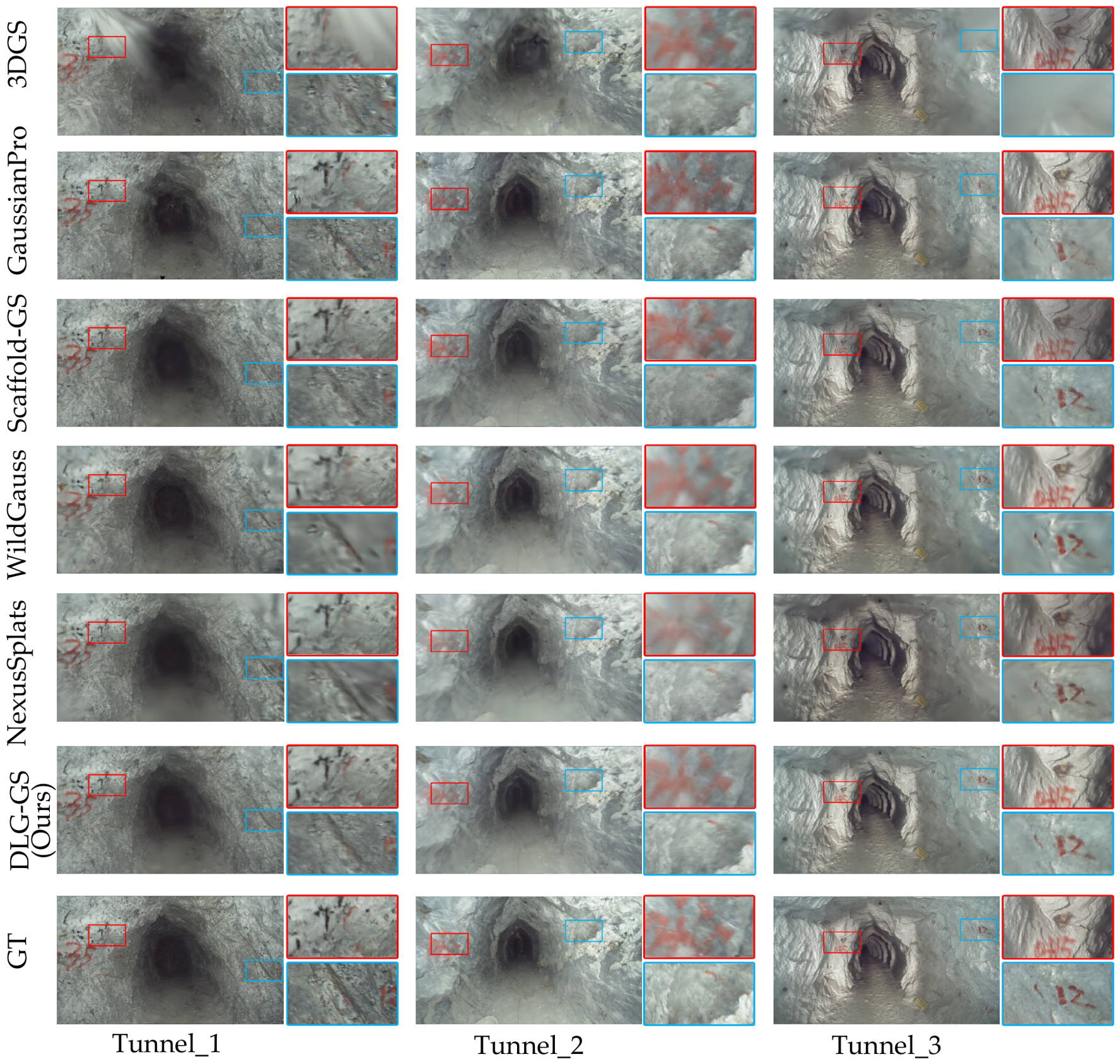
Figure 10 provides qualitative comparisons of the tunnel test scenes. Compared with several baselines, the proposed method generally shows clearer local texture recovery and fewer visible artifacts in shadowed or weakly constrained regions. In the enlarged areas, NexusSplats tends to exhibit blur or color deviation, whereas our method preserves more stable local detail and appearance consistency.

3.4.2. Public Dataset

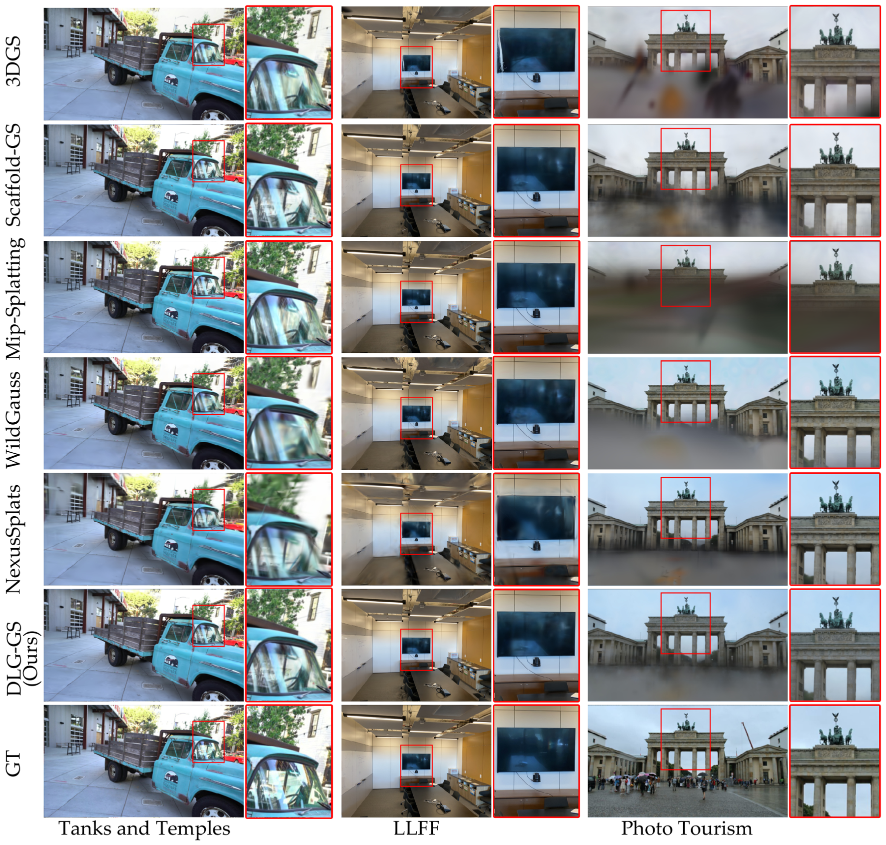
To further examine the behavior of the proposed method beyond the tunnel setting, we evaluate it on selected scenes from three public benchmarks: Tanks and Temples, LLFF, and Photo Tourism. The quantitative results are reported in

Table 2. Quantitative comparison of rendering quality on selected scenes from the Tanks and Temples [51], LLFF [52], and Photo Tourism datasets [53]. (The symbol ↓ indicates that lower values in that column represent better quality, while ↑ indicates that higher values represent better quality. Best results per column are bolded; second-best are underlined).

Methods	GPU h/FPS	Tanks and Temples			LLFF			Photo Tourism
		PSNR ↑	SSIM ↑	LPIPS ↓	PSNR ↑	SSIM ↑	LPIPS ↓	PSNR ↑	SSIM ↑	LPIPS ↓
NeRF	>10/<1	21.0746	0.7634	0.2759	28.3708	0.8428	0.2719	14.4048	0.6067	0.4809
3DGS	0.27/102	24.8474	0.8617	0.1588	31.8008	0.9512	0.1343	16.5302	0.7483	0.3197
GaussianPro	0.32/98	23.3371	0.7052	0.4115	30.9268	0.9460	0.1367	16.6577	0.7517	0.3185
Scaffold-GS	0.30/95	25.1026	0.8627	0.1544	33.5998	0.9610	0.1098	17.2014	0.7672	0.2997
2DGS	0.33/100	24.5804	0.8535	0.1824	28.4300	0.9345	0.1749	17.0199	0.7599	0.3132
Mip-Splatting	0.36/126	25.1033	0.8730	0.1288	33.2610	0.9643	0.0679	15.2936	0.7189	0.3503
SSS	1.22/28	25.0805	0.8686	0.1208	32.6911	0.9576	0.1025	10.8454	0.5658	0.5435
WildGaussians	1.45/29	23.4230	0.7910	0.2139	28.5508	0.9484	0.1312	19.1844	0.7827	0.3348
NexusSplats	0.92/48	22.1526	0.7277	0.3058	25.9311	0.9426	0.4195	19.3614	0.7725	0.3337
Ours	1.13/41	25.7103	0.8652	0.1576	33.8096	0.9601	0.1143	20.3193	0.7971	0.2836

. Overall, the proposed method achieves the highest PSNR on the three selected scenes, with values of 25.71 dB, 33.81 dB, and 20.32 dB, respectively. These results suggest that the proposed framework remains effective outside the tunnel setting, although the magnitude of improvement is generally smaller than that observed on the tunnel dataset.

More specifically, on the selected Tanks and Temples scene, our method achieves the highest PSNR, while SSIM and LPIPS remain competitive but are not the best among all methods. On the selected LLFF scene, our method again obtains the highest PSNR, but the differences relative to Scaffold-GS and Mip-Splatting are small, and the best SSIM and LPIPS are achieved by other baselines. On the selected Photo Tourism scene, the proposed method achieves the best results on all three metrics, indicating stronger adaptation under larger appearance variation, illumination inconsistency, and occlusion.

Taken together, these results provide complementary evidence that the proposed method can transfer to selected non-tunnel scenes, while also indicating that its gains are more pronounced in the tunnel-oriented setting considered in this work. Therefore, the public-dataset results are better interpreted as supporting transferability rather than establishing broad scene-independent generalization.

Figure 11 shows qualitative comparisons of the selected public scenes. On the Tanks and Temples scene, the proposed method preserves fine local structures, such as thin wires and edges. On the LLFF scene, the rendered result is visually close to the reference image, although small deviations remain in specular or reflective regions. On the Photo Tourism scene, the proposed method produces a more consistent appearance under larger illumination and viewpoint variation.

3.5. Ablation Experiments

To evaluate the respective roles of DLAAM and VDJC, we conducted ablation experiments on the tunnel dataset using four configurations: the baseline without the two proposed modules, the baseline with only VDJC, the baseline with only DLAAM, and the full model with both modules enabled. The results are summarized in

Table 3. Rendering results for different module combinations of the tunnel dataset (The symbol ↓ indicates that lower values in that column represent better quality, while ↑ indicates that higher values represent better quality. Best results per column are bolded; second-best are underlined).

Scene/Metrics	Tunnel_1			Tunnel_2			Tunnel_3
	PSNR ↑	SSIM ↑	LPIPS ↓	PSNR ↑	SSIM ↑	LPIPS ↓	PSNR ↑	SSIM ↑	LPIPS ↓
Base	26.0471	0.7827	0.3934	26.1402	0.8173	0.4117	23.4969	0.7224	0.4538
Only VDJC	26.1597	0.7874	0.3900	26.2456	0.8178	0.4118	23.6018	0.7248	0.4507
Only DLAAM	26.7035	0.7900	0.3928	27.3773	0.8253	0.4093	24.3969	0.7307	0.4531
Ours	26.8275	0.7895	0.3899	27.4617	0.8259	0.4059	24.5368	0.7333	0.4561

.

Overall, the ablation results show that DLAAM contributes a larger and more consistent improvement in image-level rendering quality across the three tunnel scenes. In comparison, the effect of VDJC alone is more moderate, but it still provides positive changes in several cases, particularly in terms of structural stability and perceptual behavior in weakly constrained regions. This difference suggests that the appearance-adaptive component is the primary driver of the quantitative gains, while the depth-related constraint mainly plays a complementary regularization role.

When both modules are enabled, the full model achieves the strongest overall PSNR performance and remains highly competitive in SSIM and LPIPS across the three scenes. At the same time, the full model is not uniformly optimal for every metric in every scene, indicating that the contributions of the two modules are not identical and may vary with scene characteristics and evaluation criteria. Therefore, the ablation results are better interpreted as supporting a complementary interaction between DLAAM and VDJC, rather than a uniformly dominant gain across all settings.

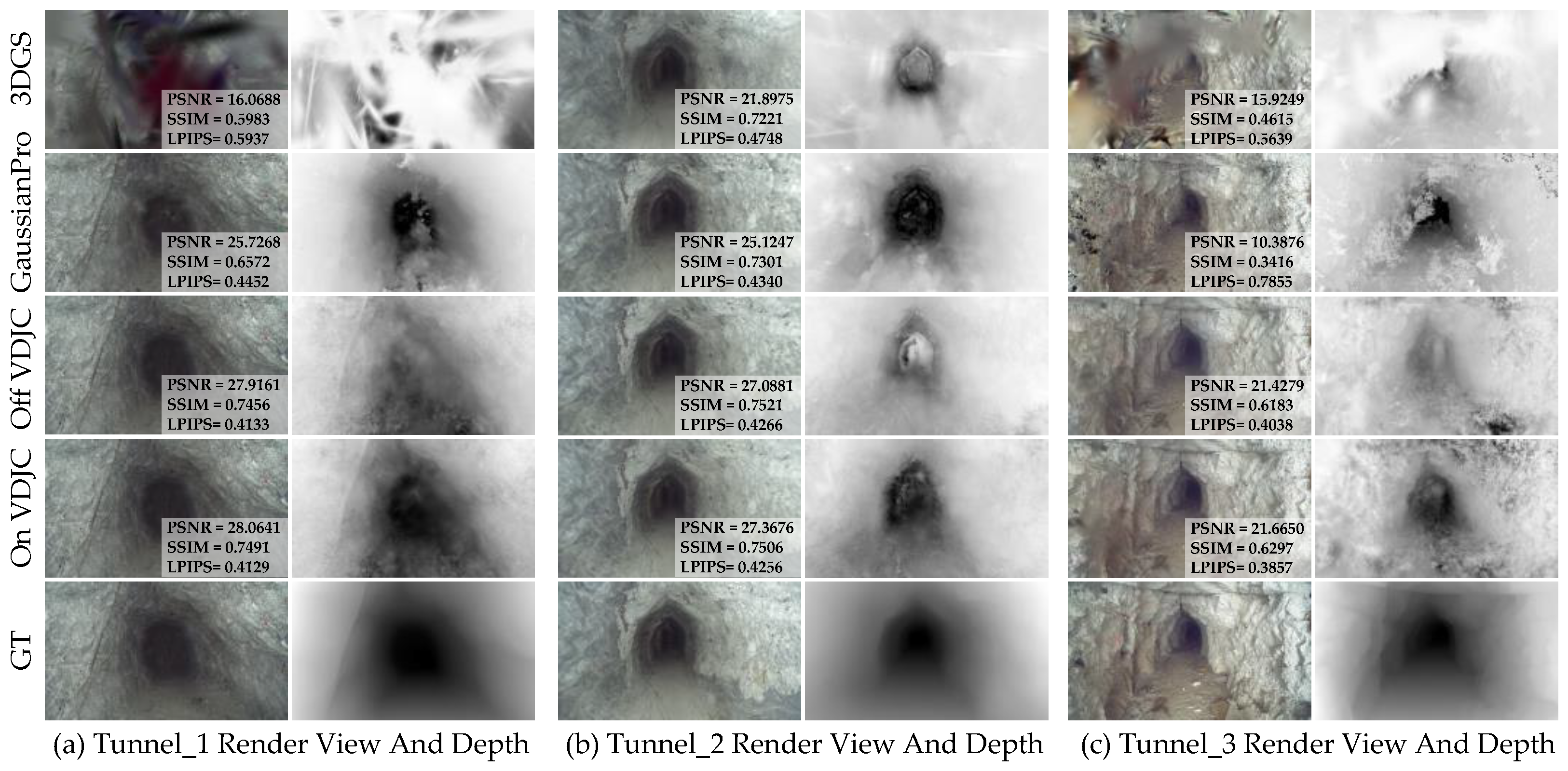
To further illustrate the role of VDJC, we compared the rendered views and rendered-depth visualizations with VDJC disabled and enabled. As shown in Figure 12, we also included 3DGS and GaussianPro as additional references for comparison in the tunnel scene. Without explicit depth regularization, 3DGS exhibits more noticeable floating artifacts in the rendered image, and its rendered-depth map shows larger deviations from the monocular depth reference. GaussianPro reduces some of these unstable responses through depth-based regularization, but texture degradation can still be observed in several rendered regions. By comparison, enabling VDJC leads to more stable rendered-depth behavior and reduced local inconsistencies in weakly textured areas. These qualitative observations suggest that the combination of neural-Gaussian-level local constraint and voxel-anchor-level structural constraint helps improve rendered-depth consistency and suppress local floating artifacts under weak geometric constraints, thereby contributing to a more stable and spatially plausible Gaussian representation.

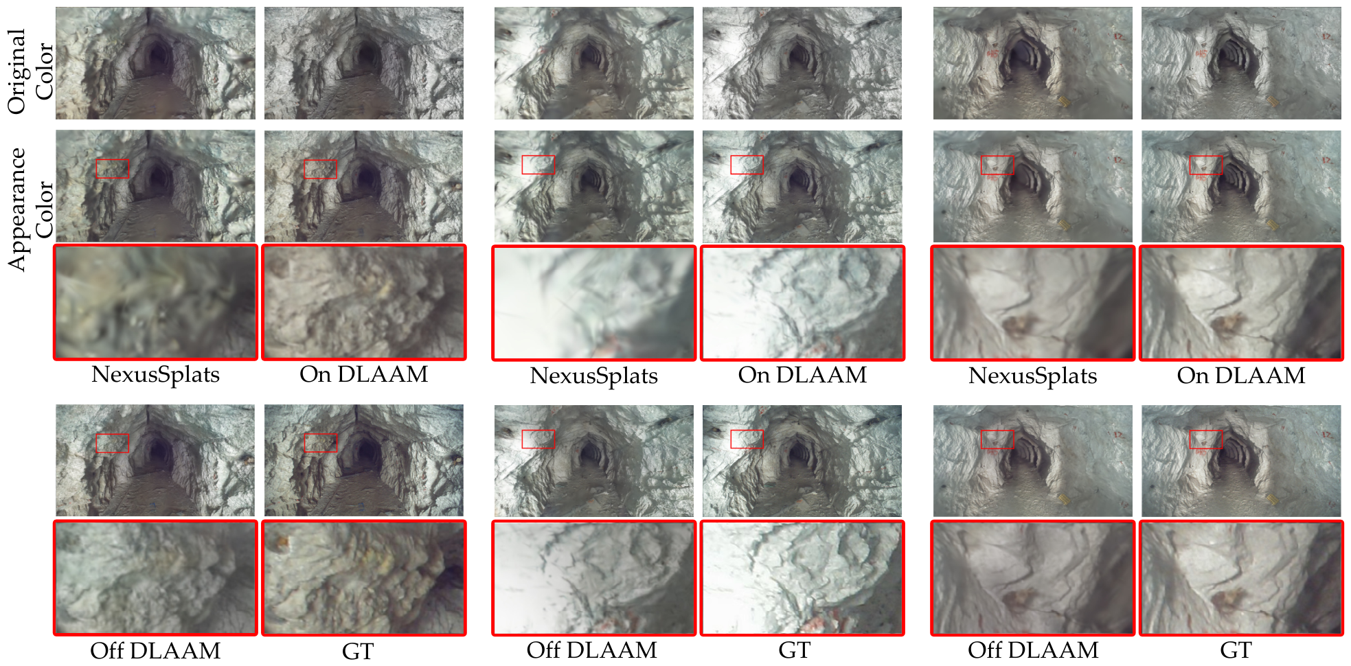
To qualitatively illustrate the effect of DLAAM, we compared rendered results with the appearance modeling branch disabled and enabled, using NexusSplats as a reference baseline. As shown in Figure 13, the rendered views with DLAAM are generally closer to the ground-truth images in color appearance than those obtained without appearance modeling, especially in the highlighted regions. Compared with the rendered results of NexusSplats, the views produced with DLAAM also preserve clearer local texture expression in several regions.

Figure 13 further compares the rendered results obtained using the original color prediction and the appearance-adaptive color prediction. Without DLAAM, the rendered views tend to exhibit a relatively fixed color tendency across different viewpoints, making it more difficult to reflect local illumination variation. After enabling DLAAM, the rendered appearance becomes more consistent with the observed view-specific lighting, particularly in warm-toned illuminated areas, shadow transition regions, and local bright spots, where the output is visually closer to the reference images. These qualitative comparisons suggest that DLAAM helps the model better accommodate dynamic lighting variation while maintaining more stable local appearance expression.

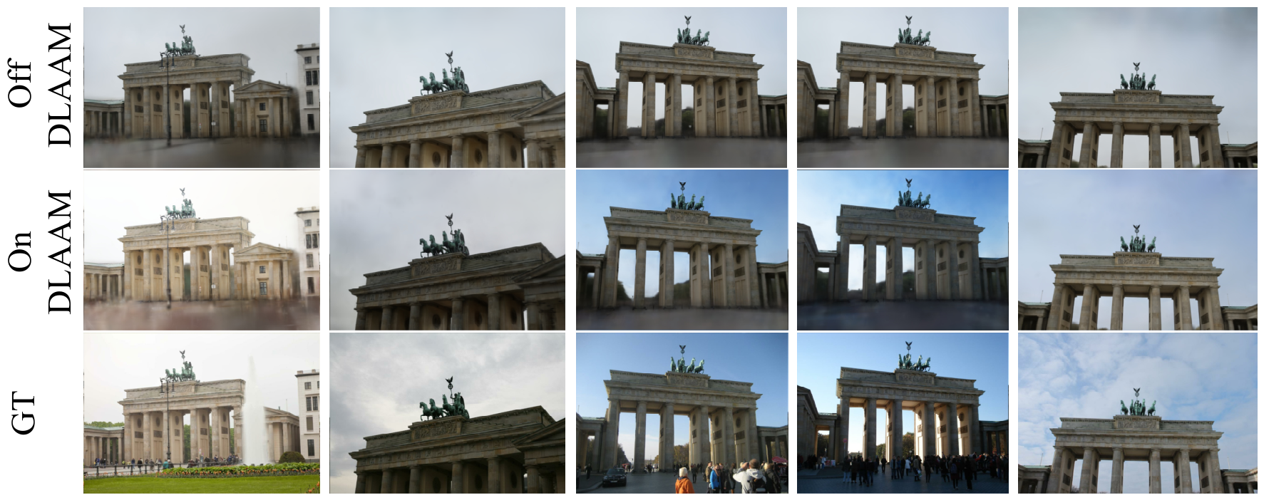
To further illustrate the qualitative effect of DLAAM in a scene with noticeable cross-view illumination variation, we present rendered results on the Photo Tourism dataset with and without the appearance modeling branch. As shown in Figure 14, enabling DLAAM produces renderings that are generally more consistent with the reference images in terms of color appearance, while still preserving local texture details in several regions. These visual comparisons suggest that DLAAM can provide useful appearance adaptation beyond the tunnel dataset, particularly in scenes with evident view-dependent lighting variation.

4. Discussion

4.1. Overall Performance and Comparison in Tunnel Scene

Across the three tunnel scenes considered in this study, DLG-GS shows clear improvements over the selected baselines in overall rendering quality. As reported in Table 1, the proposed method achieves the highest PSNR and SSIM in all three scenes, while also remaining competitive in LPIPS. These results indicate that the proposed appearance adaptation and depth-guided spatial regularization are beneficial for tunnel-oriented reconstruction under the evaluated dynamic-lighting and weakly constrained conditions.

Compared with standard 3DGS, DLG-GS produces more stable rendered views with fewer visible floating artifacts and better color consistency in shadowed or locally illuminated regions. Relative to Scaffold-GS, the gains suggest that the additional appearance modeling and depth-guided regularization provide useful complementary information beyond the voxel-anchored neural Gaussian representation. Compared with NexusSplats and WildGaussians, which also address cross-view appearance variation, DLG-GS achieves stronger overall performance on the three tunnel scenes, particularly in PSNR and SSIM, while providing visually more stable local appearance in the qualitative comparisons.

Overall, these results support the view that jointly considering illumination-related appearance variation and weakly constrained spatial regularization is helpful for the tunnel scenes studied in this work. At the same time, the improvements should be interpreted within the scope of the current evaluation setting, which remains focused on a limited number of tunnel scenes.

4.2. Generalization to Public Benchmarks

On the public benchmarks considered in this study, DLG-GS remains competitive and shows scene-dependent improvements beyond the tunnel setting. As reported in Table 2, the proposed method achieves the best PSNR on the selected Tanks and Temples, LLFF, and Photo Tourism scenes, while SSIM and LPIPS improvements are less uniform across datasets. This pattern suggests that the proposed appearance adaptation and depth-guided spatial regularization are not limited to tunnel scenes alone, although their benefits on public benchmarks depend more strongly on scene characteristics and imaging conditions.

In the Tanks and Temples scene, DLG-GS improves PSNR, although the LPIPS advantage is less pronounced, and some thin protruding structures in the background remain difficult to reconstruct accurately.

In the LLFF scene, the gain in PSNR is relatively small, while SSIM and LPIPS are slightly weaker than those of some competing methods. This behavior is consistent with the fact that LLFF contains more forward-facing views and comparatively milder illumination variation, where the baseline methods already perform strongly and where reflective regions may still introduce local deviations.

In contrast, the Photo Tourism scene shows a clearer benefit from the proposed appearance modeling, which is consistent with its stronger cross-view illumination variation. At the same time, NexusSplats remains competitive in some regions and may produce fewer artifacts in several occlusion-sensitive areas, indicating that the advantage of DLG-GS is not uniform across all public-scene conditions.

Overall, these results suggest that DLG-GS has promising transferability beyond the tunnel dataset, especially in scenes with more noticeable appearance variation, while also indicating that its improvements on public benchmarks are more moderate than those observed in the tunnel evaluation. In terms of efficiency, the additional DLAAM and VDJC modules introduce extra computational cost, although the rendering speed remains above 40 FPS in all tested public scenes, preserving the real-time characteristic of Gaussian splatting.

4.3. Effectiveness of the Proposed Modules

The ablation study in Table 3 indicates that the two modules make different contributions to the overall framework. Among them, DLAAM leads to more stable gains across the three tunnel scenes, suggesting that appearance adaptation is the dominant factor in improving rendering quality under dynamic lighting. In contrast, the effect of VDJC is more dependent on scene characteristics and becomes more visible in Scene 2, where shadow coverage and weak-texture effects are stronger. Although the full model achieves the highest PSNR in all three scenes, it is not uniformly best across all reported metrics. Therefore, the results are better interpreted as showing that DLAAM and VDJC provide complementary benefits rather than a uniformly dominant joint advantage. Consistent with this observation, the qualitative comparisons show that VDJC mainly improves rendered-depth stability and reduces local floating artifacts, whereas DLAAM mainly improves appearance consistency across views with different illumination conditions.

4.4. Limitations and Future Work

Despite the encouraging results, this study still has several limitations. First, the tunnel evaluation remains limited in scale, as it is conducted on three self-collected scenes with test views sampled from the same acquisition sequences. Although this setting is useful for controlled comparison, it is still a relatively limited test of generalization under broader tunnel conditions and more diverse lighting patterns.

Second, the current validation is primarily rendering-oriented. The reported metrics, including PSNR, SSIM, and LPIPS, mainly evaluate rendered-view fidelity and perceptual quality. In addition, monocular depth is used in this work as a regularization prior to stabilize Gaussian optimization rather than as geometric ground truth. Accordingly, the current experiments mainly support improved rendered-depth consistency, spatial stability, and geometric plausibility of the learned representation, rather than a strict measurement of physical geometric accuracy.

Third, the current tunnel dataset does not provide independent high-precision geometric ground truth. Consequently, geometry-specific indicators, such as depth RMSE with respect to ground-truth geometry, point-cloud or mesh accuracy, normal consistency, and tunnel-specific geometric inspection metrics, are not reported in this work. Such evaluations would be necessary for studies whose primary objective is geometry accuracy benchmarking, and they remain an important direction for future validation.

Finally, on datasets such as LLFF, local deviations can still be observed in regions with strong specular highlights, suggesting that the current appearance modeling remains sensitive to non-Lambertian reflectance. In addition, the extra DLAAM and VDJC modules introduce additional training cost compared with the base 3DGS framework, even though real-time rendering is still maintained.

Future work will therefore focus on four directions: expanding the tunnel evaluation to more scenes and more diverse acquisition conditions; introducing geometry-specific validation, such as depth error, point-based geometric consistency, or other structural metrics; improving the handling of specular and other non-Lambertian appearance effects through more expressive reflectance-aware modeling; and reducing computational overhead through lighter attention designs, more efficient anchor management, or model compression. In addition, it would also be valuable to further examine the transferability of the framework to other low-texture and illumination-varying engineering environments, such as corridors, underground facilities, or industrial spaces.

5. Conclusions

This paper presents DLG-GS, a 3D Gaussian splatting framework designed for tunnel-oriented reconstruction under dynamic lighting and weakly constrained conditions. To address the coupled effects of cross-view appearance variation and unstable spatial optimization in shadow-induced weak-texture regions, the framework integrates two components: DLAAM for lighting-adaptive appearance modeling and VDJC for depth-prior-guided spatial regularization. Within a unified voxel-based Gaussian representation, these two components jointly improve appearance consistency and reconstruction stability under the evaluated conditions.

Experimental results on the self-collected tunnel dataset show that DLG-GS achieves clear improvements over the selected baselines in PSNR and SSIM, while remaining competitive in LPIPS and maintaining real-time rendering performance. From a rendering-oriented perspective, these results support the effectiveness of the proposed method and suggest improved rendered-view fidelity and spatial stability of the learned Gaussian representation under challenging imaging conditions. Additional experiments on several public benchmark scenes further suggest that the proposed design has promising transferability beyond the tunnel setting, although the gains on those datasets are more moderate and more scene-dependent than those observed in the tunnel evaluation.

Several limitations remain. The current tunnel evaluation is limited in scale, and the validation is mainly based on rendering-oriented metrics rather than independent geometry-specific measurements. In addition, the present appearance modeling remains sensitive to strong specular highlights in some scenes, and the additional modules introduce extra training cost. Future work will therefore focus on broader tunnel evaluation, geometry-oriented validation with independent ground truth, improved handling of non-Lambertian appearance effects, and more efficient lightweight implementations for practical deployment in complex engineering environments.

References

1. Fabbri, S.; Sauro, F.; Santagata, T.; Rossi, G.; De Waele, J. High-resolution 3-D mapping using terrestrial laser scanning as a tool for geomorphological and speleogenetical studies in caves: An example from the Lessini mountains (North Italy). Geomorphology 2017, 280, 16–29. [Google Scholar] [CrossRef]
2. Hu, T.; Sun, X.; Su, Y.; Guan, H.; Sun, Q.; Kelly, M.; Guo, Q. Development and Performance Evaluation of a Very Low-Cost UAV-Lidar System for Forestry Applications. Remote Sens. 2021, 13, 77. [Google Scholar] [CrossRef]
3. Kedziorski, P.; Jagoda, M.; Tysiac, P.; Katzer, J. An Example of Using Low-Cost LiDAR Technology for 3D Modeling and Assessment of Degradation of Heritage Structures and Buildings. Materials 2024, 17, 5445. [Google Scholar] [CrossRef] [PubMed]
4. Forster, C.; Pizzoli, M.; Scaramuzza, D. SVO: Fast Semi-Direct Monocular Visual Odometry. In Proceedings of the IEEE International Conference on Robotics and Automation (ICRA), Hong Kong, China, 31 May–7 June 2014; pp. 15–22. [Google Scholar]
5. Wang, R.; Schwörer, M.; Cremers, D. Stereo DSO: Large-Scale Direct Sparse Visual Odometry with Stereo Cameras. In Proceedings of the IEEE International Conference on Computer Vision (ICCV), Venice, Italy, 22–29 October 2017; pp. 3923–3931. [Google Scholar]
6. Wang, W.; Min, H.; Wu, X.; Yang, L.; Yan, C.; Fang, Y.; Zhao, X. LGD: A fast place recognition method based on the fusion of local and global descriptors. Expert Syst. Appl. 2024, 251, 123996. [Google Scholar] [CrossRef]
7. Zhao, Z.; Song, T.; Xing, B.; Lei, Y.; Wang, Z. PLI-VINS: Visual-Inertial SLAM Based on Point-Line Feature Fusion in Indoor Environment. Sensors 2022, 22, 5457. [Google Scholar] [CrossRef] [PubMed]
8. Zhao, Z.; Liu, Q.; Zhu, J.; Yao, Z.; Lu, Y.; Li, Q. FIGS-SLAM: Gaussian splatting SLAM with dynamic frequency control and influence-based pruning. Expert Syst. Appl. 2025, 294, 128763. [Google Scholar] [CrossRef]
9. Cadena, C.; Carlone, L.; Carrillo, H.; Latif, Y.; Scaramuzza, D.; Neira, J.; Reid, I.; Leonard, J.J. Past, Present, and Future of Simultaneous Localization and Mapping: Toward the Robust-Perception Age. IEEE Trans. Robot. 2016, 32, 1309–1332. [Google Scholar] [CrossRef]
10. Barron, J.T.; Mildenhall, B.; Verbin, D.; Srinivasan, P.P.; Hedman, P. Zip-NeRF: Anti-Aliased Grid-Based Neural Radiance Fields. In Proceedings of the IEEE/CVF International Conference on Computer Vision (ICCV), Paris, France, 2–6 October 2023; pp. 19640–19648. [Google Scholar]
11. Mildenhall, B.; Srinivasan, P.P.; Tancik, M.; Barron, J.T.; Ramamoorthi, R.; Ng, R. NeRF: Representing Scenes as Neural Radiance Fields for View Synthesis. Commun. ACM 2022, 65, 99–106. [Google Scholar] [CrossRef]
12. Xu, Q.; Xu, Z.; Philip, J.; Bi, S.; Shu, Z.; Sunkavalli, K.; Neumann, U. Point-NeRF: Point-based Neural Radiance Fields. In Proceedings of the IEEE/CVF Conference on Computer Vision and Pattern Recognition (CVPR), New Orleans, LA, USA, 18–24 June 2022; pp. 5428–5438. [Google Scholar]
13. Yu, A.; Ye, V.; Tancik, M.; Kanazawa, A. pixelNeRF: Neural Radiance Fields from One or Few Images. In Proceedings of the IEEE/CVF Conference on Computer Vision and Pattern Recognition (CVPR), Nashville, TN, USA, 20–25 June 2021; pp. 4576–4585. [Google Scholar]
14. Barron, J.T.; Mildenhall, B.; Tancik, M.; Hedman, P.; Martin-Brualla, R.; Srinivasan, P.P. Mip-NeRF: A Multiscale Representation for Anti-Aliasing Neural Radiance Fields. In Proceedings of the IEEE/CVF International Conference on Computer Vision (ICCV), Virtual, 11–17 October 2021; pp. 5835–5844. [Google Scholar]
15. Fridovich-Keil, S.; Meanti, G.; Warburg, F.R.; Recht, B.; Kanazawa, A. K-Planes: Explicit Radiance Fields in Space, Time, and Appearance. In Proceedings of the IEEE/CVF Conference on Computer Vision and Pattern Recognition (CVPR), Vancouver, BC, Canada, 18–22 June 2023; pp. 12479–12488. [Google Scholar]
16. Liu, L.; Gu, J.; Lin, K.Z.; Chua, T.-S.; Theobalt, C. Neural Sparse Voxel Fields. In Proceedings of the Conference on Neural Information Processing Systems (NeurIPS), Vancouver, BC, Canada, 6–12 December 2020; pp. 15651–15663. [Google Scholar]
17. Sun, C.; Sun, M.; Chen, H.-T. Direct Voxel Grid Optimization: Super-fast Convergence for Radiance Fields Reconstruction. In Proceedings of the IEEE/CVF Conference on Computer Vision and Pattern Recognition (CVPR), New Orleans, LA, USA, 18–24 June 2022; pp. 5449–5459. [Google Scholar]
18. Kerbl, B.; Kopanas, G.; Leimkuehler, T.; Drettakis, G. 3D Gaussian Splatting for Real-Time Radiance Field Rendering. ACM Trans. Graph. 2023, 42, 1–14. [Google Scholar] [CrossRef]
19. Rückert, D.; Franke, L.; Stamminger, M. ADOP: Approximate Differentiable One-Pixel Point Rendering. ACM Trans. Graph. 2022, 41, 1–14. [Google Scholar] [CrossRef]
20. Wang, Y.; Serena, F.; Wu, S.; Öztireli, C.; Sorkine-Hornung, O. Differentiable Surface Splatting for Point-based Geometry Processing. ACM Trans. Graph. 2019, 38, 1–14. [Google Scholar] [CrossRef]
21. Kopanas, G.; Philip, J.; Leimkühler, T.; Drettakis, G. Point-Based Neural Rendering with Per-View Optimization. Comput. Graph. Forum 2021, 40, 29–43. [Google Scholar] [CrossRef]
22. Huang, B.; Yu, Z.; Chen, A.; Geiger, A.; Gao, S. 2D Gaussian Splatting for Geometrically Accurate Radiance Fields. In Proceedings of the SIGGRAPH Conference on Emerging Technologies, Denver, CO, USA, 27 July–1 August 2024; pp. 1–11. [Google Scholar]
23. Zhu, J.; Yue, J.; He, F.; Wang, H. 3D Student Splatting and Scooping. In Proceedings of the IEEE/CVF Conference on Computer Vision and Pattern Recognition (CVPR), Nashville, TN, USA, 11–15 June 2025; pp. 21045–21054. [Google Scholar]
24. Navaneet, K.L.; Meibodi, K.P.; Koohpayegani, S.A.; Pirsiavash, H. CompGS: Smaller and Faster Gaussian Splatting with Vector Quantization. In Proceedings of the European Conference on Computer Vision (ECCV), Milan, Italy, 29 September–4 October 2024; pp. 330–349. [Google Scholar]
25. Niedermayr, S.; Stumpfegger, J.; Westermann, R. Compressed 3D Gaussian Splatting for Accelerated Novel View Synthesis. In Proceedings of the IEEE/CVF Conference on Computer Vision and Pattern Recognition (CVPR), Seattle, WA, USA, 17–21 June 2024; pp. 10349–10358. [Google Scholar]
26. Girish, S.; Gupta, K.; Shrivastava, A. EAGLES: Efficient Accelerated 3D Gaussians with Lightweight EncodingS. In Proceedings of the European Conference on Computer Vision (ECCV), Milan, Italy, 29 September–4 October 2024; pp. 54–71. [Google Scholar]
27. Kerbl, B.; Meuleman, A.; Kopanas, G.; Wimmer, M.; Lanvin, A.; Drettakis, G. A Hierarchical 3D Gaussian Representation for Real-Time Rendering of Very Large Datasets. ACM Trans. Graph. 2024, 43, 1–15. [Google Scholar] [CrossRef]
28. Fan, Z.; Wang, K.; Wen, K.; Zhu, Z.; Xu, D.; Wang, Z. LightGaussian: Unbounded 3D Gaussian Compression with 15x Reduction and 200+ FPS. In Proceedings of the Conference on Neural Information Processing Systems (NeurIPS), Vancouver, BC, Canada, 10–15 December 2024; pp. 140138–140158. [Google Scholar]
29. Yu, Z.; Chen, A.; Huang, B.; Sattler, T.; Geiger, A. Mip-Splatting: Alias-free 3D Gaussian Splatting. In Proceedings of the IEEE/CVF Conference on Computer Vision and Pattern Recognition (CVPR), Seattle, WA, USA, 17–21 June 2024; pp. 19447–19456. [Google Scholar]
30. Lu, T.; Yu, M.; Xu, L.; Xiangli, Y.; Wang, L.; Lin, D.; Dai, B. Scaffold-GS: Structured 3D Gaussians for View-Adaptive Rendering. In Proceedings of the IEEE/CVF Conference on Computer Vision and Pattern Recognition (CVPR), Seattle, WA, USA, 17–21 June 2024; pp. 20654–20664. [Google Scholar]
31. Lin, J.; Li, Z.; Huang, B.; Tang, X.; Liu, J.; Liu, S.; Wu, X.; Song, F.; Yang, W. Decoupling Appearance Variations with 3D Consistent Features in Gaussian Splatting. In Proceedings of the AAAI Conference on Artificial Intelligence (AAAI), Philadelphia, PA, USA, 25 February–4 March 2025; pp. 5236–5244. [Google Scholar]
32. Chen, X.; Zhang, Q.; Li, X.; Chen, Y.; Feng, Y.; Wang, X.; Wang, J. Hallucinated Neural Radiance Fields in the Wild. In Proceedings of the IEEE/CVF Conference on Computer Vision and Pattern Recognition (CVPR), New Orleans, LA, USA, 18–24 June 2022; pp. 12933–12942. [Google Scholar]
33. Rudnev, V.; Elgharib, M.; Smith, W.; Liu, L.; Golyanik, V.; Theobalt, C. NeRF for Outdoor Scene Relighting. In Proceedings of the European Conference on Computer Vision (ECCV), Tel Aviv, Israel, 23–27 October 2022; pp. 615–631. [Google Scholar]
34. Martin-Brualla, R.; Radwan, N.; Sajjadi, M.S.M.; Barron, J.T.; Dosovitskiy, A.; Duckworth, D. NeRF in the Wild: Neural Radiance Fields for Unconstrained Photo Collections. In Proceedings of the IEEE/CVF Conference on Computer Vision and Pattern Recognition (CVPR), Virtual, 19–25 June 2021; pp. 7206–7215. [Google Scholar]
35. Meshry, M.; Goldman, D.B.; Khamis, S.; Hoppe, H.; Pandey, R.; Snavely, N.; Martin-Brualla, R. Neural Rerendering in the Wild. In Proceedings of the IEEE/CVF Conference on Computer Vision and Pattern Recognition (CVPR), Long Beach, CA, USA, 16–20 June 2019; pp. 6878–6880. [Google Scholar]
36. Zhang, T.; Huang, K.; Zhi, W.; Johnson-Roberson, M. DarkGS: Learning Neural Illumination and 3D Gaussians Relighting for Robotic Exploration in the Dark. In Proceedings of the IEEE/RSJ International Conference on Intelligent Robots and Systems, Abu Dhabi, United Arab Emirates, 14–18 October 2024; pp. 12864–12871. [Google Scholar]
37. Tang, Y.; Xu, D.; Hou, Y.; Gong, Y.; Wang, Z. NexusSplats: An Efficient Approach for Robust Novel View Synthesis from Unstructured Image Collections. In Proceedings of the International Conference on Machine Intelligence and Nature-Inspired Computing (MIND), Xiamen, China, 31 October–2 November 2025; pp. 144–149. [Google Scholar]
38. Gao, J.; Gu, C.; Lin, Y.; Li, Z.; Zhu, H.; Cao, X.; Zhang, L.; Yao, Y. Relightable 3D Gaussians: Realistic Point Cloud Relighting with BRDF Decomposition and Ray Tracing. In Proceedings of the European Conference on Computer Vision (ECCV), Milan, Italy, 29 September–4 October 2024; pp. 73–89. [Google Scholar]
39. Lin, J.; Li, Z.; Tang, X.; Liu, J.; Liu, S.; Liu, J.; Lu, Y.; Wu, X.; Xu, S.; Yan, Y.; et al. VastGaussian: Vast 3D Gaussians for Large Scene Reconstruction. In Proceedings of the IEEE/CVF Conference on Computer Vision and Pattern Recognition (CVPR), Seattle, WA, USA, 17–21 June 2024; pp. 5166–5175. [Google Scholar]
40. Xu, J.; Mei, Y.; Patel, V.M. Wild-GS: Real-Time Novel View Synthesis from Unconstrained Photo Collections. In Proceedings of the Conference on Neural Information Processing Systems (NeurIPS), Vancouver, BC, Canada, 10–15 December 2024; pp. 103334–103355. [Google Scholar]
41. Kulhanek, J.; Peng, S.; Kukelova, Z.; Pollefeys, M.; Sattler, T. WildGaussians: 3D Gaussian Splatting in the Wild. In Proceedings of the Conference on Neural Information Processing Systems (NeurIPS), Vancouver, BC, Canada, 10–15 December 2024; pp. 21271–21288. [Google Scholar]
42. Chung, J.; Oh, J.; Lee, K.M. Depth-Regularized Optimization for 3D Gaussian Splatting in Few-Shot Images. In Proceedings of the IEEE/CVF Conference on Computer Vision and Pattern Recognition Workshops (CVPRW), Seattle, WA, USA, 17–18 June 2024; pp. 811–820. [Google Scholar]
43. Li, J.; Zhang, J.; Bai, X.; Zheng, J.; Ning, X.; Zhou, J.; Gu, L. DNGaussian: Optimizing Sparse-View 3D Gaussian Radiance Fields with Global-Local Depth Normalization. In Proceedings of the IEEE/CVF Conference on Computer Vision and Pattern Recognition (CVPR), Seattle, WA, USA, 17–21 June 2024; pp. 20775–20785. [Google Scholar]
44. Cheng, K.; Long, X.; Yang, K.; Yao, Y.; Yin, W.; Ma, Y.; Wang, W.; Chen, X. GaussianPro: 3D Gaussian Splatting with Progressive Propagation. In Proceedings of the International Conference on Machine Learning (ICML), Vienna, Austria, 21–27 July 2024; pp. 8123–8140. [Google Scholar]
45. Xiong, H.; Muttukuru, S.; Upadhyay, R.; Chari, P.; Kadambi, A. SparseGS: Sparse View Synthesis Using 3D Gaussian Splatting. In Proceedings of the International Conference on 3D Vision (3DV), Singapore, 25–28 March 2025; pp. 1032–1041. [Google Scholar]
46. Wang, Z.; Bovik, A.C.; Sheikh, H.R.; Simoncelli, E.P. Image Quality Assessment: From Error Visibility to Structural Similarity. IEEE Trans. Image Process. 2004, 13, 600–612. [Google Scholar] [CrossRef] [PubMed]
47. Yang, L.; Kang, B.; Huang, Z.; Zhao, Z.; Xu, X.; Feng, J.; Zhao, H. Depth Anything V2. In Proceedings of the Conference on Neural Information Processing Systems (NeurIPS), Vancouver, BC, Canada, 10–15 December 2024; pp. 21875–21911. [Google Scholar]
48. Jin, J.; Li, X.; Huang, H.; Liu, L.; Sun, Y.; Liu, B. PEP-GS: Perceptually-Enhanced Precise Structured 3D Gaussians for View-Adaptive Rendering. arXiv 2024. [Google Scholar] [CrossRef]
49. Yan, Q.; Feng, Y.; Zhang, C.; Pang, G.; Shi, K.; Wu, P.; Dong, W.; Sun, J.; Zhang, Y. HVI: A New Color Space for Low-light Image Enhancement. In Proceedings of the IEEE/CVF Conference on Computer Vision and Pattern Recognition (CVPR), Nashville, TN, USA, 11–15 June 2025; pp. 5678–5687. [Google Scholar]
50. Xu, Y.; Wang, L.; Chen, M.; Ao, S.; Li, L.; Guo, Y. DropoutGS: Dropping Out Gaussians for Better Sparse-view Rendering. In Proceedings of the IEEE/CVF Conference on Computer Vision and Pattern Recognition (CVPR), Nashville, TN, USA, 11–15 June 2025; pp. 701–710. [Google Scholar]
51. Knapitsch, A.; Park, J.; Zhou, Q.-Y.; Koltun, V. Tanks and Temples: Benchmarking Large-scale Scene Reconstruction. ACM Trans. Graph. 2017, 36, 1–13. [Google Scholar] [CrossRef]
52. Mildenhall, B.; Srinivasan, P.P.; Ortiz-Cayon, R.; Kalantari, N.K.; Ramamoorthi, R.; Ng, R.; Kar, A. Local Light Field Fusion: Practical View Synthesis with Prescriptive Sampling Guidelines. ACM Trans. Graph. 2019, 38, 1–14. [Google Scholar] [CrossRef]
53. Snavely, N.; Seitz, S.M.; Szeliski, R. Photo Tourism: Exploring Photo Collections in 3D. ACM Trans. Graph. 2006, 25, 835–846. [Google Scholar] [CrossRef]
54. Schönberger, J.L.; Frahm, J.-M. Structure-from-Motion Revisited. In Proceedings of the IEEE Conference on Computer Vision and Pattern Recognition (CVPR), Las Vegas, NV, USA, 27–30 June 2016; pp. 4104–4113. [Google Scholar]
Figure 1. The impact of dynamic lighting on novel view rendering of scenes. (a) Novel view rendering in an outdoor scene; (b) novel view rendering in a tunnel scene. The “Input View” refers to the input training views, and different training views exhibit appearance variations. The “Render View” is the novel view rendered image, which often shows significant differences from the “Ground Truth” reference image.
Remotesensing 18 01705 g001
Figure 2. Comparison of rendered images with depth images. (a) Comparison of view and depth view for an indoor scene; (b) comparison of view and depth view for a tunnel scene. “Render View” is the rendered image, compared with the “Ground Truth” reference image. “Render Depth View” is the rendered depth image, compared with the “Reference Depth” reference depth image. There is distortion at the positions marked by red circles.
Remotesensing 18 01705 g002
Figure 3. A comparison of texture rendering across different 3DGS methods (the blue box marks the floating artifacts, and the red box indicates the level of textural detail). (a) Rendered view of 3DGS; (b) rendered view of GaussianPro; (c) rendered view of NexusSplats; (d) Ground Truth.
Remotesensing 18 01705 g003
Figure 4. The overall pipeline of DLG-GS is illustrated in the framework diagram. (a) Building upon the neural Gaussian representation; (b) VDJC workflow; (c) DLAAM workflow.
Remotesensing 18 01705 g004
Figure 5. Generate a neural Gaussian from anchor points. For k neural Gaussians, their properties (opacity, color, scale, and quaternion) are decoded using F α , F c , F s , and F q from anchor features, the relative viewing direction from the camera to the anchor point, and distance. The final image is rendered via alpha-blending.
Remotesensing 18 01705 g005
Figure 6. DLAAM dynamic prediction of neural Gaussian appearance color.
Remotesensing 18 01705 g006
Figure 7. Workflow of the local multi-granularity attention mechanism.
Remotesensing 18 01705 g007
Figure 8. MLP f network structure.
Remotesensing 18 01705 g008
Figure 9. Tunnel data collection. A six-monocular-pinhole-camera array arranged in the front, top, left, left-upper, right, and right-upper orientations is rigidly mounted on a unified photogrammetric rig with integrated active illumination, enabling robust image acquisition in low-light tunnel environments.
Remotesensing 18 01705 g009
Figure 10. Qualitative comparison of rendered images on the tunnel test dataset (The red and blue squares in the figure are enlarged annotations for image comparison).
Remotesensing 18 01705 g010
Figure 11. Qualitative comparisons on public datasets. Our method maintains high-fidelity rendering quality on the Tanks and Temples and LLFF benchmarks, while also producing visually consistent results on the Photo Tourism dataset (The red boxes in the figure are enlarged local annotations for image comparison).
Remotesensing 18 01705 g011
Figure 12. Comparison of rendered views and depth views. (a) Rendered view and depth map of tunnel scene Tunnel_1; (b) rendered view and depth map of tunnel scene Tunnel_2; (c) rendered view and depth map of tunnel scene Tunnel_3. We selected “3DGS” and “GaussianPro” for comparison and compared the rendered views and depth views of our method with VDJC activated (On VDJC) and VDJC deactivated (Off VDJC). The evaluation metrics and their values for the rendered images are annotated in the figure.
Remotesensing 18 01705 g012
Figure 13. Comparison of rendered views with respect to the appearance model. We compared these with “NexusSplats” and present the rendered views of our method with DLAAM activated (On DLAAM) and deactivated (Off DLAAM) against the ground truth “GT”. Additionally, we compared the rendered views obtained using “Appearance Color” and “Original Color” for both “NexusSplats” and our “On DLAAM”. Regions with noticeable color changes are marked in the figure.
Remotesensing 18 01705 g013
Figure 14. Comparison of rendered views under different camera positions. “Off DLAAM”—without the appearance model; “On DLAAM”—with the appearance model; “GT”—the ground truth image.
Remotesensing 18 01705 g014