A Waterfall-Plot-Based Multi-Criteria Framework for X-Ray Pulsar Time-Delay Estimation in Multi-Scenario Celestial Remote Sensing and Navigation

Highlights

What are the main findings?

• A waterfall-plot-based multi-criteria framework is proposed for X-ray pulsar time-delay estimation, integrating structural saliency, principal-projection saliency, and geometric consistency for robust period discrimination.
• The proposed method significantly improves the accuracy and stability of X-ray pulsar time-delay estimation compared with benchmark statistical-test-based methods using Insight-HXMT satellite observation data.
• An end-to-end simulation framework is established for multi-scenario celestial remote sensing and navigation, enabling full-chain validation from photon observation to final navigation performance.

What are the implications of the main findings?

• The proposed framework provides a robust way to extract pulsar measurement information from X-ray pulsar observations under complex observation conditions.
• Improved time-delay estimation can effectively enhance navigation performance in typical deep-space mission scenarios, including Earth orbit, Earth–Moon transfer, and Mars approach.
• The proposed method shows strong potential for long-duration autonomous deep-space remote sensing and navigation applications.

Abstract

To improve the accuracy and stability of X-ray pulsar time-delay estimation for multi-scenario celestial remote sensing and navigation, this paper proposes a time-delay estimation method based on a waterfall-plot multi-criteria framework and develops an end-to-end simulation framework for multi-scenario applications. First, a pulsar profile waterfall-plot model is built, and principal component analysis is performed to characterize candidate periodic structures. The contribution rate of the principal eigenvalue is used to describe the overall significance of the candidate period, and the projection variance of the first principal component is used to measure the prominence of the candidate pattern in the principal subspace. Second, support vector regression is used to fit the peak track of the waterfall plot, and a regression slope is used to describe the geometric stability of the candidate period. These three indicators are fused for pulsar period and time-delay estimation. Tests based on Insight-HXMT satellite observation data show that, compared with the ${\chi }^2$ and $Z^2$ test methods, our method improves time-delay estimation accuracy by 68.68% and 50.43%, respectively. Multi-scenario navigation simulations indicate positioning improvements of approximately 0.83 km, 3.04 km, and 1.05 km in the Earth-orbiting, Earth–Moon transfer, and Mars approach scenarios, respectively. These results suggest that the proposed framework can improve pulsar time-delay estimation and may provide useful measurement support for celestial remote sensing and navigation.

1. Introduction

Celestial remote sensing-based navigation is an autonomous navigation approach in which a spacecraft determines its attitude, position, and velocity by observing natural celestial bodies such as stars, planets, or pulsars and utilizing their spatial positions, radiation characteristics, and period stability [1,2,3,4]. Among them, pulsar navigation, as an emerging celestial ranging and positioning technology, can provide spacecraft with a stable spatiotemporal reference and potentially ultra-high positioning accuracy, and it is regarded as one of the most promising celestial navigation technologies for autonomous exploration missions in multiple flight phases, such as cruise, approach, and orbiting phases [5,6]. In a pulsar navigation system, the spacecraft orbital dynamics equation is usually adopted as the state model, while pulsar time-delay measurements serve as observations. Estimation algorithms such as the Kalman filter are then employed to fuse the system state and measurement information, thereby achieving spacecraft navigation and positioning. Therefore, the accuracy of pulsar time-delay estimation directly affects the positioning performance of the navigation system [7,8].

First, with regard to the acquisition of time-delay measurements in pulsar navigation, pulsar time-delay refers to the time difference between the arrival of a pulsar signal at the spacecraft and its arrival at the solar system barycenter reference position [9]. Owing to the highly stable periodic characteristics of pulsar radiation, pulsar time-delay is usually estimated by comparing the phase offset between the signal received by the spacecraft and the standard pulsar signal at the solar system barycenter. However, under actual observation conditions, the radiation intensity of pulsars in the X-ray band is weak, and the signal within a single period is difficult to be directly resolved by the detector. Therefore, it is usually necessary to estimate the pulsar period in real time and, combined with signal enhancement techniques such as the epoch-folding algorithm, reconstruct the pulsar periodic signal [10,11,12]. In this process, the accuracy of period estimation directly affects the quality of the folded profile, and it further determines the accuracy of phase-delay and time-delay estimation. It can thus be seen that, period estimation is thus a key step in obtaining reliable pulsar time-delay measurements.

Existing period estimation methods mainly include single-statistical-test methods, fast-search methods, and multi-information-assisted methods. Early studies mainly used single statistical quantities as the criterion for candidate-period discrimination. Leahy et al. [13] proposed using the ${\chi }^2$ test as the objective function to select the candidate period with the highest folded-profile significance. Buccheri et al. [14] proposed the $Z^2$ statistic, which is more sensitive to the signal profile. Subsequently, Bélanger, Huppenkothen, Bachetti, Xie, and others [15,16,17,18] improved and simplified the $Z^2$ statistic. In addition, Xie et al. [19] further incorporated profile peak features and proposed an improved Rayleigh test statistic. These methods are simple to compute and have a wide range of applicability. However, they usually rely on a single significance indicator, and the use of structural consistency and phase-drift information in segmented folded profiles is still insufficient. In recent years, some studies have introduced more profile information or data-driven features to improve period estimation performance. Song et al. [20,21] proposed improved fast-folding algorithms and the BPF-FFA method, which improved the efficiency of period search. Liu et al. [22] and Wang et al. [23] carried out period estimation from the perspectives of compressed sensing and equal-photon-number segment distribution, respectively. Ma et al. [24] transformed pulsar profiles into two-dimensional images and combined them with a convolutional neural network for period estimation. Zhao et al. [25] used a Transformer network for pulsar phase estimation, which also provides a similar idea for data-driven feature learning in period estimation. These studies show that profile morphology, image representation, and data-driven features can provide effective information for period estimation. However, some methods still depend on prior knowledge, standard templates, or training samples, and their interpretability and cross-source applicability remain limited. It is worth noting that, unlike the above methods centered on single-significance data, Cassanelli et al. [26] proposed a waterfall-plot–principal component analysis (PCA) method, which jointly discriminates candidate periods from the two aspects of signal significance and phase consistency. This indicates that the two-dimensional structural information in segmented folded profiles has application potential for period estimation. However, this method mainly relies on the structural information obtained from principal component analysis, and it still makes insufficient use of the different representations of the dominant structure in the waterfall plot and the geometric drift of the peak trajectory.

Second, with regard to the application simulation of pulsar navigation methods in multi-mission scenarios, existing studies have carried out relatively extensive exploration of the system modeling and performance validation of pulsar navigation for different flight phases and orbital environments. In terms of application scenarios, these studies mainly cover typical mission phases such as the Earth-orbiting phase and Earth–Moon transfer phase, as well as the deep-space cruise, planetary approach, and orbiting phases [27,28,29,30]. However, existing studies on multi-scenario application simulation still have two deficiencies. First, although existing work covers multiple types of mission phases, most of it is conducted under a single mission background, lacking a unified review and systematic comparison of typical scenarios such as Earth orbiting, Earth–Moon transfer, and planetary approach missions and thus making it difficult to comprehensively analyze the applicability boundaries of pulsar navigation methods under different orbital scales, dynamical characteristics, and observation geometry conditions. Second, in the design of simulation chains, existing studies usually perform statistical modeling directly on pulsar measurement information and directly use it as the input to navigation filtering, lacking a full-process closed-loop simulation framework from detector observation data simulation, pulsar period estimation, and profile reconstruction to time-delay acquisition and final navigation and positioning solutions. Therefore, such methods can hardly reflect, in a real and accurate manner, the propagation effect of measurement-information estimation errors on final navigation performance. In particular, under a pure pulsar navigation scheme, the performance of period estimation and time-delay information acquisition directly determines the positioning accuracy and robustness of the system. Therefore, it is necessary to establish a full-chain simulation framework for multiple typical mission scenarios so as to achieve a unified evaluation of pulsar time-delay information estimation methods and their value in navigation applications.

To address the above problems, we propose a time-delay estimation method based on a waterfall-plot multi-criteria framework and develop an end-to-end simulation framework for multi-scenario celestial remote sensing and navigation. First, for pulsar photon sequences, a profile waterfall-plot representation is constructed. By folding the observation data with candidate periods, the observation data are mapped into a two-dimensional phase-time space, and the observation task is jointly modeled from the two aspects of amplitude significance and phase consistency. Subsequently, PCA is performed on the waterfall-plot model to extract low-dimensional dominant structural features. On the one hand, the contribution rate of the principal eigenvalue is taken as Criterion 1 to characterize the overall significance of the candidate period structure. On the other hand, the projection variance of the principal component is taken as Criterion 2 to measure the prominence of the candidate period pattern in the principal subspace. Meanwhile, for the geometric consistency characteristics exhibited by the candidate-period stripes in the waterfall plot, the peak trajectory of the folded profile is extracted, and a support vector regression (SVR) model is adopted to fit the peak trajectory. The regression slope is then taken as Criterion 3 to characterize the consistency and stability of the candidate period structure in a geometric sense. On this basis, a multi-criteria fusion framework is constructed to comprehensively evaluate candidate periods, thereby achieving robust estimation of the pulsar period and reconstructing the pulsar profile accordingly. Finally, combined with the cross-correlation algorithm, the high-performance acquisition of pulsar time-delay information is achieved.

The main contributions are summarized as follows:

• A pulsar time-delay estimation method based on a waterfall-plot multi-criteria framework is proposed. By constructing a pulsar profile waterfall-plot model, periodic structural features are extracted from multiple perspectives, including the contribution of the principal eigenvalue, the saliency of the principal projection, and the geometric consistency of the peak trajectory.
• The proposed method is evaluated using Insight-HXMT on-orbit observation data of the Crab pulsar. The results show that, under the tested observation conditions, the proposed method reduces the time-delay estimation error and improves estimation stability compared with existing benchmark methods.
• End-to-end simulation is conducted for multi-scenario pulsar navigation applications. The proposed method is applied to multiple typical pulsar navigation mission scenarios, including the Earth-orbiting phase, the Earth–Moon transfer phase, and the Mars approach phase. The simulations are used to analyze how improvements in pulsar time-delay estimation propagate to navigation performance under different orbital scales and observation geometries.

2. Pulsar Time-Delay Estimation Method

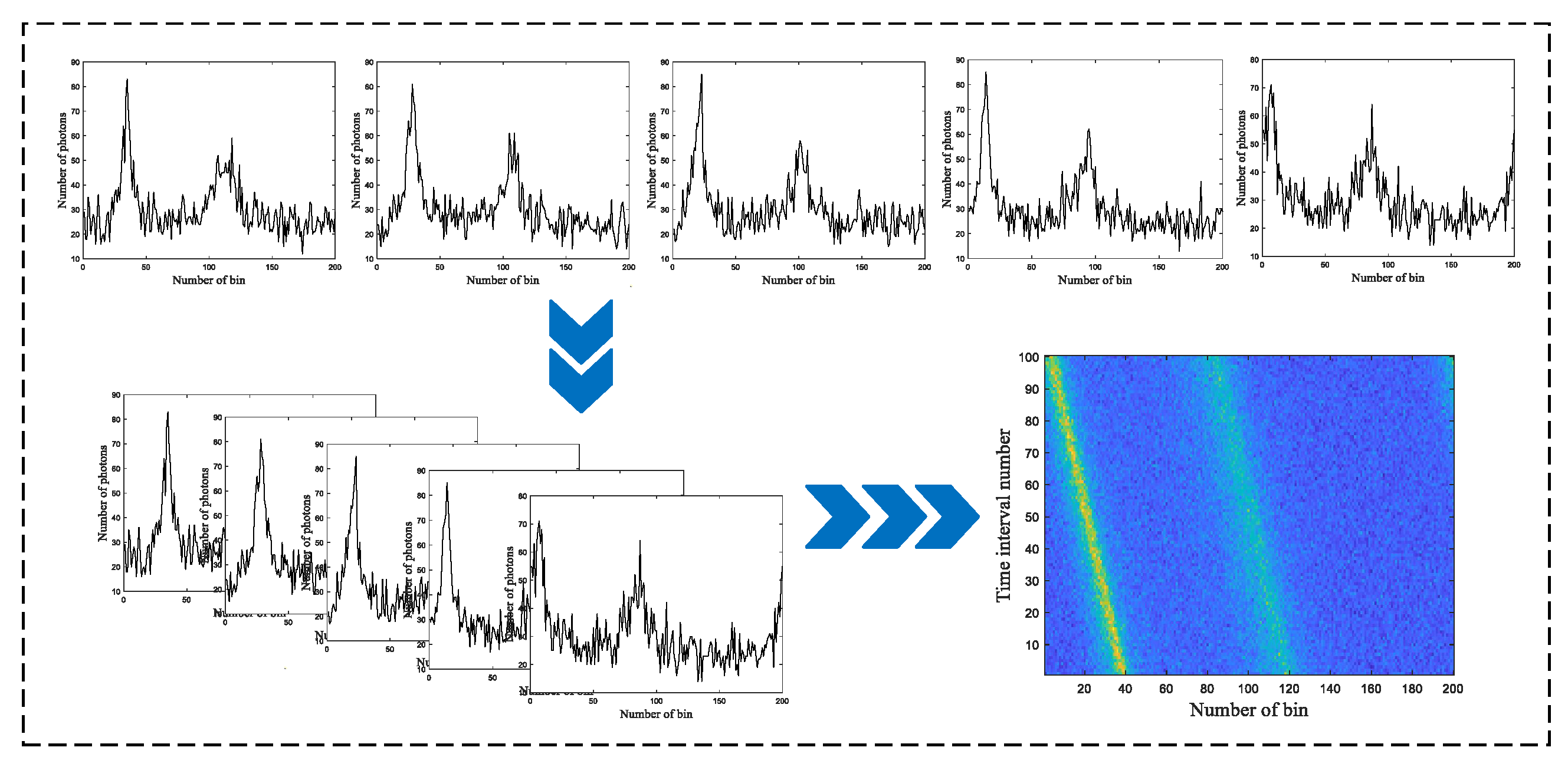
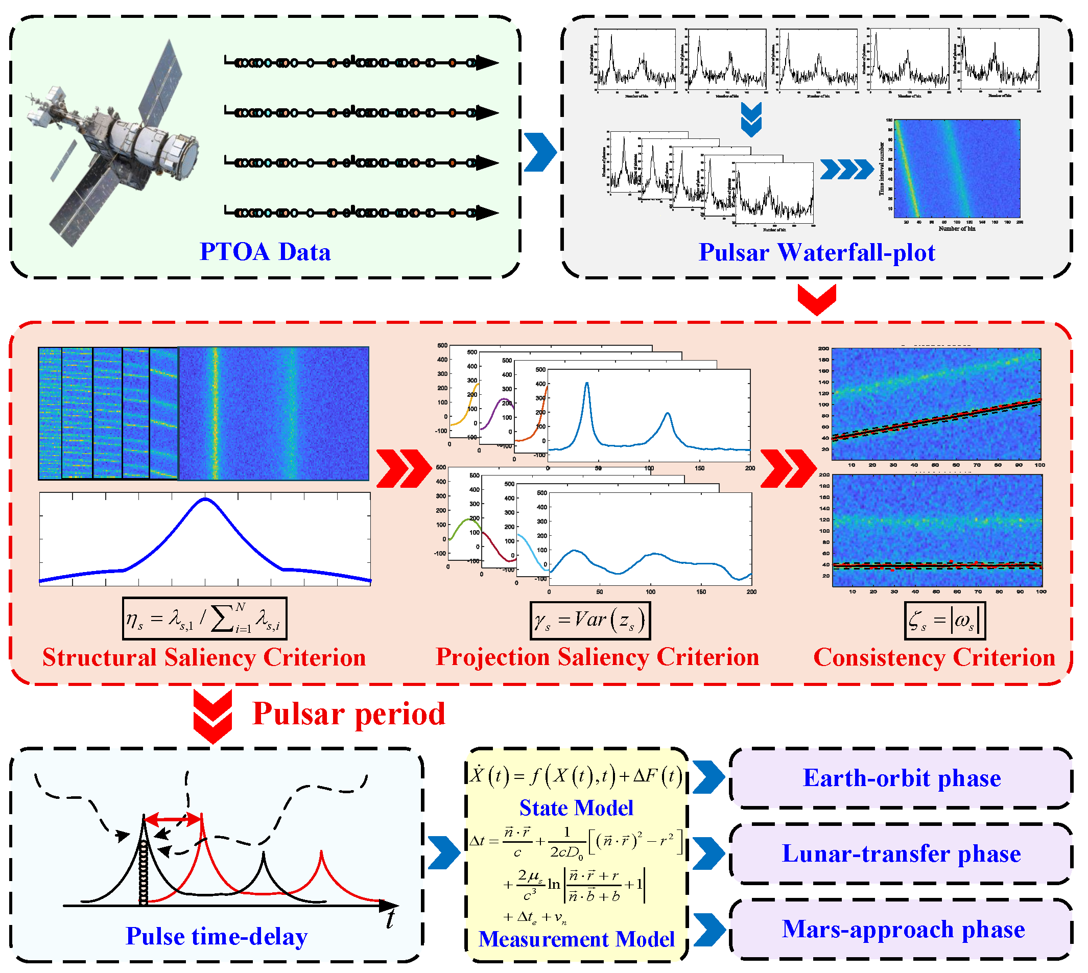
In this section, a pulsar profile waterfall-plot model is first established. Next, based on waterfall-plot principal component analysis and support vector regression, a multi-criteria discrimination framework for pulsar period estimation is established from different perspectives, including the significance of the reduced-dimensional structure, the stability of the principal projection in the reduced-dimensional space, and geometric consistency. Finally, the folded profile is reconstructed using the estimated period, and the corresponding phase-delay and time-delay are modeled and calculated. The specific framework of the time-delay estimation method is shown in Figure 1.

2.1. Profile Waterfall-Plot Model

Traditional profile folding methods mainly adopt the epoch-folding algorithm; that is, all observed events are folded into the same period according to a candidate period so as to achieve signal enhancement. The candidate period is then judged to be optimal or not by testing the significance of the folded signal. The profile waterfall-plot folding method is also developed on this basis. In this method, the observed events are divided into several sub-event segments and folded simultaneously by epoch folding, and the folded profiles are combined into a three-dimensional structure. Candidate periods are discriminated by examining the significance and phase consistency of the folded signal.

Specifically, the total observation time is equally divided into M segments, and the observation duration of each segment is Ts. The pulsar folding period (i.e., the candidate period) is denoted by Ps. The observation time of each segment is then equally divided into $N_T$ segments, and each divided segment is further equally divided into N bins according to $T_{bin}$s. Then, the X-ray pulsar signal profile model obtained for each observation task segment by using the epoch-folding method can be expressed as follows:

$$\begin{array}{cc}\hfill & r\left(a_{t_i}\right)={\displaystyle \frac{\frac{1}{N_T}{\sum }_{j=1}^{N_T}{P}_j\left(t_i\right)}{{\sum }_{k=1}^N\left(\frac{1}{N_T}{\sum }_{j=1}^{N_T}{P}_j\left(t_k\right)\right)}},\hfill \\ \hfill & a=1,2,\dots ,M,i=1,2,\dots ,N.\hfill \end{array}$$

(1)

where $P_j\left(t_i\right)$ denotes the photon information value in the i-th bin of the j-th time segment.

The normalized folded profiles are then encoded in chronological order. By constructing the mapping relationship between the color scale and the profile signal intensity, the pulsar profile waterfall plot under the candidate period can be obtained. The profile waterfall-plot model can be expressed as follows:

$$W\in {\mathbb{R}}^{M\times N}$$

(2)

The modeling process of the pulsar profile waterfall plot is shown in Figure 2.

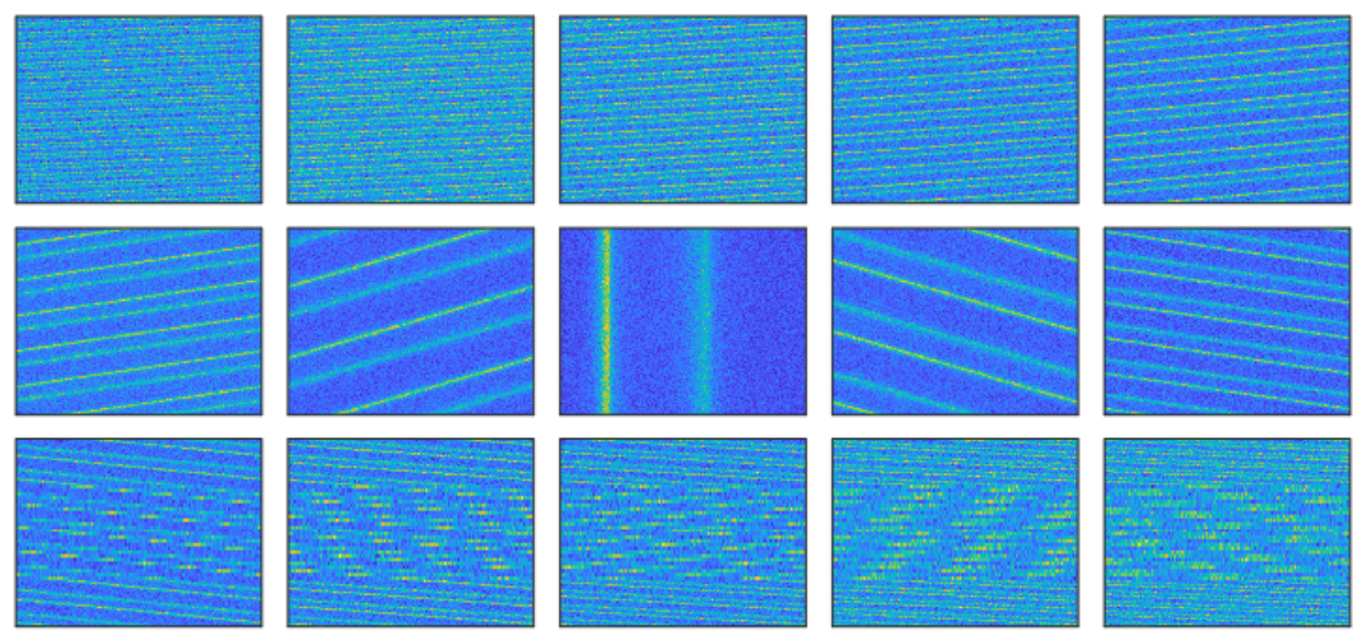
Figure 3 shows the profile waterfall plots of the Crab pulsar obtained by folding with different candidate periods. It can be seen from the figure that, when the difference between the candidate period and the true period is large, the profile waterfall plot exhibits a disordered distribution. As the candidate period gradually approaches the true period, the significance of the folded profile gradually increases, and the phase of the folded profile gradually tends to become consistent. When the candidate period is equal to the true period, the folded profile has the strongest significance, and the phase distribution is basically the same, which is manifested as a clear three-dimensional image with vertically distributed geometric stripes.

The traditional epoch-folding algorithm can only determine whether a candidate period is optimal through the significance of the folded signal. In contrast, the profile waterfall-plot model can perform joint discrimination from the two aspects of signal significance and phase consistency, thereby fully exploiting pulsar photon information and showing considerable application potential for subsequently improving the estimation accuracy of pulsar time-delay estimation.

2.2. Significance Criterion Based on Principal Component Analysis

2.2.1. Structural Significance Criterion

The structural differences of profile waterfall plots under different candidate periods are mainly reflected in the phase correlation among folded profiles. Principal component analysis can extract the principal directions in which variations are most concentrated in an image through the covariance structure. Therefore, it is suitable for describing the overall structural characteristics of profile waterfall plots and can quantitatively analyze the structural significance of profile waterfall plots under different candidate periods.

Specifically, let the profile waterfall plot constructed under the s-th candidate period $P_s$ be denoted by $W_s$. It is first necessary to perform centering on it, namely,

$$X_s=W_s-{\mathbf{1}}_M{\mu }_s,{\mu }_s={\displaystyle \frac{1}{M}}{\mathbf{1}}_M^T{W}_s$$

(3)

where ${\mu }_s\in {\mathbb{R}}^{1\times N}$ denotes the mean vector of each bin.

Let $u\in {\mathbb{R}}^N$ be the projection vector along a certain direction. Then, the projection of the waterfall plot along this direction can be expressed as

$$z_s=X_{s}u$$

(4)

PCA seeks the direction along which the projection variance of the waterfall plot is maximized so as to preserve the principal variation information in the original data as much as possible [31,32]. Therefore, the optimal projection direction can be expressed as the following constrained optimization problem.

$$\underset{u}{max}{\displaystyle \frac{1}{M}}{z}_s^T{z}_s\mathrm{s}.\mathrm{t}.u^{T}u=1$$

(5)

Substituting Equation (4) into Equation (5), we obtain

$$\underset{u}{max}{\displaystyle \frac{1}{M}}{\left(X_{s}u\right)}^T\left(X_{s}u\right)=\underset{u}{max}{u}^T{\Sigma }_{s}u,{\Sigma }_s={\displaystyle \frac{1}{M}}{X}_s^T{X}_s$$

(6)

where ${\Sigma }_s$ is the covariance matrix of the waterfall plot. To solve the constrained optimization problem in Equation (6), the Lagrangian function can be constructed as

$$L(u,\lambda )=u^T{\Sigma }_{s}u-\lambda (u^{T}u-1)$$

(7)

By taking the derivative of Equation (7) and calculating the stationary point, we obtain

$${\Sigma }_{s}u=\lambda u$$

(8)

It can thus be seen that the optimal projection direction corresponds to the eigenvector of the covariance matrix ${\Sigma }_s$, and the corresponding eigenvalue $\lambda$ represents the degree of variation of the waterfall plot along that direction.

Let ${\lambda }_{s,1}\ge {\lambda }_{s,2}\ge \dots \ge {\lambda }_{s,N}\ge 0$ be the eigenvalues of ${\Sigma }_s$. The first principal component corresponds to the largest eigenvalue ${\lambda }_{s,1}$, which reflects the strength of the most dominant structural information in the profile waterfall plot. In this section, in order to characterize the relative contribution of the dominant structure in the overall eigenvalues, the structural significance indicator under the candidate period $P_s$ is defined as the contribution rate of the principal eigenvalue, namely,

$${\eta }_s={\displaystyle \frac{{\lambda }_{s,1}}{{\sum }_{i=1}^N{\lambda }_{s,i}}}$$

(9)

where the contribution rate of the principal eigenvalue can reflect the concentration degree of the dominant structure in the waterfall plot relative to the overall variation. When the candidate period approaches the true period, the pulse phases of different folded segments show better consistency, and the energy distribution in the waterfall plot becomes more concentrated along the dominant structural direction. Accordingly, the proportion of the first principal eigenvalue in the covariance matrix increases. In contrast, when the candidate period deviates from the true period, the pulse phases of the segmented profiles gradually become dispersed, and structural information is distributed over multiple directions, leading to a decrease in the contribution rate of the principal eigenvalue. Therefore, this indicator can be used to characterize the structural significance of the waterfall plot corresponding to the candidate period.

The structural significance criterion based on PCA can be expressed as follows:

$${\widehat{P}}_1=arg\underset{P_s}{max}{\eta }_s$$

(10)

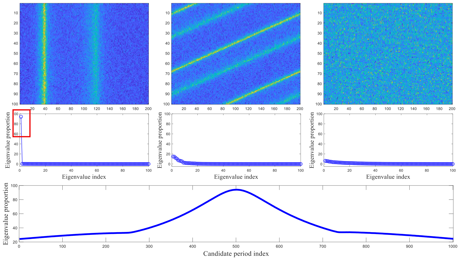
The upper panel of Figure 4 presents different profile waterfall plots and the corresponding eigenvalue contribution distributions obtained after PCA. It can be seen that, when the folding period is the true period, the contribution rate of the corresponding principal eigenvalue is significantly higher than those corresponding to the remaining eigenvalues, indicating the presence of a prominent dominant structure. When the folding period gradually deviates from the true period, however, the contribution of the principal eigenvalue of the corresponding profile waterfall plot gradually decreases to a level indistinguishable from those of the remaining eigenvalues, indicating a disordered structural distribution. The lower panel of Figure 4 shows the variation of the contribution of the principal eigenvalue during one candidate-period search process. It can be seen that the variation in the proportion of the principal eigenvalue can clearly reflect the degree of deviation between the candidate period and the true period. Therefore, the maximization of the principal eigenvalue contribution rate of the covariance matrix of the profile waterfall plot can be taken as one of the criteria for pulsar period estimation.

2.2.2. Principal-Projection Significance Criterion

In addition to quantifying the dominant structure of the profile waterfall plot from the perspective of the eigenvalue contribution rate of the covariance matrix, the significance of this dominant structure can also be described directly from the projection result along the first principal direction. On this basis, this subsection further constructs a principal-projection significance criterion based on the projection of the first principal component.

Specifically, let the first principal direction obtained by principal component analysis be $u_{s,1}$. According to Equation (4), the projection of the profile waterfall plot along this direction can be expressed as

$$z_s=X_s{u}_{s,1}$$

(11)

where $z_s\in {\mathbb{R}}^M$ is the projection-score vector of the folded profiles along the first principal direction under the s-th candidate period.

The first principal direction corresponds to the most dominant direction of variation in the profile waterfall plot, and its projection result can also directly reflect the strength of the distribution of the waterfall plot in the dominant structure. Therefore, the principal-projection significance indicator under the candidate period $P_s$ can be defined as

$${\gamma }_s=Var\left(z_s\right)$$

(12)

where $\mathrm{Var}(·)$ denotes the variance operation. When the candidate value approaches the true period, the structural features of the profile waterfall plot along the first principal direction gradually become more prominent, and the variation of the corresponding projection vector becomes more significant; accordingly, ${\gamma }_s$ takes a relatively large value. Conversely, when the candidate period gradually deviates from the true value, the dominant structure in the profile waterfall-plot weakens, and the variation amplitude of the principal projection vector decreases accordingly, causing ${\gamma }_s$ to gradually decrease.

Therefore, the principal-projection significance criterion based on PCA can be expressed as

$${\widehat{P}}_2=arg\underset{P_s}{max}{\gamma }_s$$

(13)

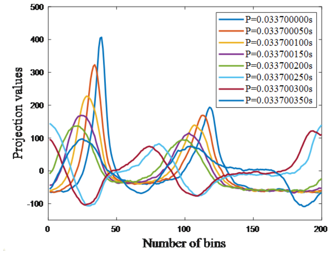
Figure 5 shows the principal projection profiles under different candidate periods. It can be seen that, as the candidate period gradually deviates from the true period, the significance of the principal projection profile indeed gradually weakens. Therefore, maximizing the significance of the projection along the principal direction of the profile waterfall plot can be taken as another criterion for pulsar period estimation.

It is worth noting that, although both the principal-projection significance criterion and the above structural significance criterion are quantitative descriptions of the dominant structure of the profile waterfall plot based on PCA, the former mainly reflects the absolute strength of the projection response along the principal direction and pays more attention to the amplitude characteristics of the dominant structure itself; the latter, through the proportion of the principal eigenvalue in the overall eigenvalues, characterizes the degree of concentration and dominance of the dominant structure relative to the overall variation. Therefore, although the two may have a certain intrinsic correlation in a statistical sense, the former preserves the absolute-strength information of the dominant mode, whereas the latter emphasizes the relative contribution of the dominant mode within the overall structure. Based on this difference in representation dimension, introducing both types of criteria simultaneously helps characterize the dominant structural features of the candidate-period waterfall plot from different perspectives, thereby improving the completeness and robustness of the discrimination results.

2.3. Geometric Consistency Criterion Based on Support Vector Regression

Section 2.2 mainly analyzes the overall statistical structural characteristics. In addition, the geometric distribution pattern of the peak points of the folded profiles in the profile waterfall plot can also reflect the degree of consistency between the candidate period and the true period. When the candidate period is close to the true period, the peak positions of the folded profiles remain stable in the phase direction, which is manifested in the waterfall plot as an approximately consistent peak-trajectory structure. Conversely, when the candidate period deviates from the true value, the peak positions undergo systematic drift, thereby forming an inclined peak trajectory. Therefore, a period criterion can be constructed based on the geometric consistency of the peak-point set.

Specifically, in the profile waterfall-plot $W_s$, M peak trajectories can be extracted, namely,

$${\left\{(x_m,y_m)\right\}}_{m=1}^M$$

(14)

where $x_m$ is the position index corresponding to the m-th folded profile, and $y_m$ is the position index of the peak point of that profile on the phase axis (to ensure that the slope of the fitting has practical meaning, the waterfall plot is transposed in this subsection).

To better characterize the overall arrangement trend of the peak-point set, this subsection uses linear support vector regression (SVR) to establish a peak-trajectory model:

$$f\left(x\right)=\omega x+b$$

(15)

where $\omega$ is the slope of the regression line, and b is the intercept.

Within the linear SVR framework, the parameter solution can be written as the following constrained optimization problem [33,34]:

$$\begin{array}{cc}\hfill \underset{\omega ,b,{\xi }_m,{\widehat{\xi }}_m}{min}& {\displaystyle \frac{1}{2}}{\parallel \omega \parallel }^2+C{\displaystyle \sum _{m=1}^M}\left({\xi }_m+{\widehat{\xi }}_m\right)\hfill \\ \hfill \mathrm{s}.\mathrm{t}.& \left\{\begin{array}{c}f\left(x_m\right)-y_m\le \epsilon +{\xi }_m\hfill \\ y_m-f\left(x_m\right)\le \epsilon +{\widehat{\xi }}_m\hfill \\ {\xi }_m,{\widehat{\xi }}_m\ge 0,m=1,2,\dots ,M\hfill \end{array}\right.\hfill \end{array}$$

(16)

where C is the penalty coefficient, $\epsilon$ is the insensitive loss function, and ${\xi }_m$ and ${\widehat{\xi }}_m$ are slack variables. This model suppresses the influence of outliers on the fitting result while ensuring the smoothness of the regression, thereby obtaining a stable linear trend of the peak-point set.

It can be seen from Equation (16) that the slope $\omega$ of the regression line directly reflects the inclination degree of the peak trajectory relative to the horizontal axis. When the candidate period is close to the true period, the fitted regression line tends to be nearly horizontal, and its slope absolute value is small. Conversely, when the candidate period deviates from the true value, the peak points drift significantly with the profile position, the inclination degree of the fitted straight line increases, and the corresponding absolute value of the slope increases. Based on this, the geometric consistency indicator under the candidate period $P_s$ is defined as

$${\zeta }_s=\left|{\omega }_s\right|$$

(17)

Therefore, the geometric consistency criterion based on SVR can be expressed as

$${\widehat{P}}_3=arg\underset{P_s}{min}{\zeta }_s$$

(18)

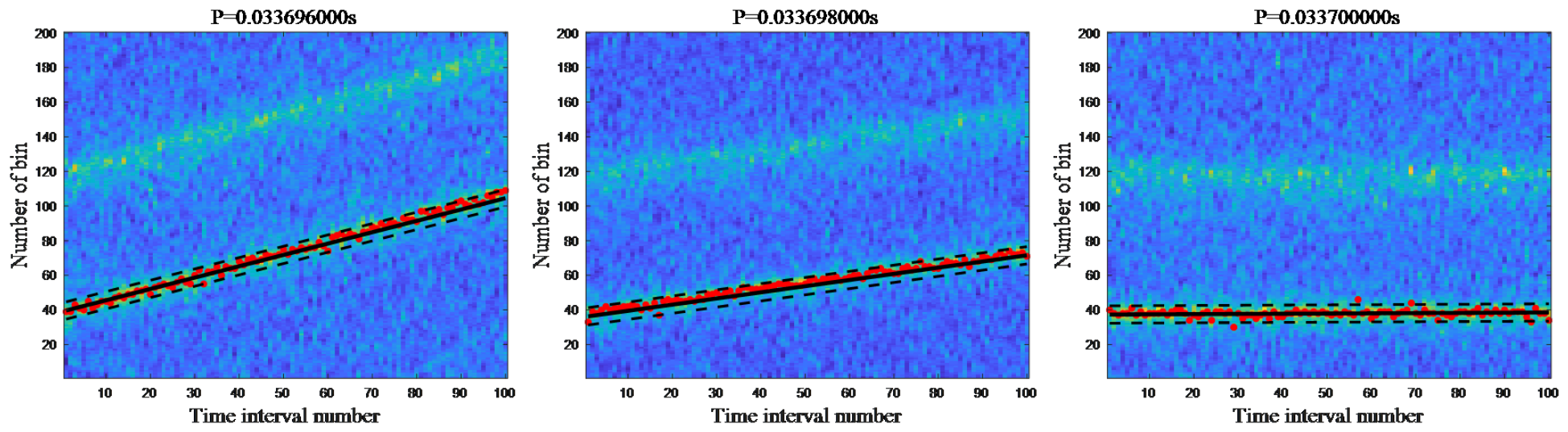
The method in this subsection proceeds directly from the geometric distribution of the peak trajectories in the profile waterfall plot, and we perform robust fitting of the peak-point set through linear SVR. As shown in Figure 6, the smaller the absolute value of the slope, the weaker the drift of the peak points along the phase direction, and the stronger the overall geometric consistency of the waterfall plot; accordingly, the corresponding candidate period is closer to the true period. Therefore, minimizing the offset of the fitted curve of the profile waterfall-plot peaks can be taken as one of the criteria for pulsar period estimation.

It is worth noting that the SVR criterion relies on the stable tracking of the same physical peak in different folded segments. To avoid switching between the main peak and the secondary peak in double-peak profiles, or false tracking caused by noise peaks, this paper adopts a local-window iterative search strategy. Specifically, the average profile is first used to determine the initial position of the peak to be tracked. Then, in each following segment, the current peak is searched within a local phase window near the peak position of the previous segment, and the window center is updated iteratively. This strategy can improve the continuity of the peak trajectory and make the SVR slope more stably reflect the phase drift caused by the candidate period. Meanwhile, within a local candidate-period search range, the candidate-period error causes continuous phase drift of the same physical peak across adjacent folded segments, and this drift can be approximated by a first-order trend. Therefore, this paper uses linear SVR to fit the main drift trend of the peak trajectory and uses the slope to represent geometric consistency. The penalty coefficient C controls the balance between the fitting error and smoothness, while the insensitive loss function $ϵ$ is used to suppress small-amplitude peak fluctuations. Together, these two parameters affect the stability of slope estimation.

2.4. Pulsar Time-Delay Information Model

As can be seen from Section 2.2 and Section 2.3, for the same candidate period, the profile waterfall plot can be used for period estimation through the structural significance criterion, the principal-projection significance criterion, and the geometric consistency criterion. In order to comprehensively utilize the characterization capability of different criteria for the true period, this subsection fuses the information from the above evaluation criteria to obtain the comprehensive estimate of the pulsar period, namely,

$$\widehat{P}={\displaystyle \frac{1}{3}}\left({\widehat{P}}_1+{\widehat{P}}_2+{\widehat{P}}_3\right)$$

(19)

where the three criteria characterize the candidate period from the perspectives of structural significance, principal-projection significance, and geometric consistency of the peak trajectory, and they are complementary to each other. Compared with weighting strategies that rely on specific samples or prior assumptions, equal-weight averaging does not introduce additional tuning parameters and can maintain the stability of the fusion process. Therefore, this paper adopts equal-weight averaging as the fusion method for the multi-criteria period estimation results.

For the estimated period $\widehat{P}$, the profile folding model in Equation (1) can be used to reconstruct the observed events and obtain the current observed profile $r\left({\varphi }_t\right)$. Furthermore, the folded profile is cross-correlated with the standard profile $s\left({\varphi }_t\right)$ at the solar system barycenter, and the phase-delay information can be expressed as

$$\Delta \varphi =arg\underset{\tau }{max}{\displaystyle \sum _{i=1}^N}r\left({\varphi }_{t_i}\right)s({\varphi }_{t_i}-\tau )$$

(20)

where ${\varphi }_{t_i}$ is the phase index of the i-th bin, and $\Delta \varphi$ is the optimal phase offset of the current observed profile relative to the standard profile.

Since the phase offset obtained by cross-correlation matching reflects only the fractional delay within one period, the total time-delay of the pulsar can be expressed as

$$\Delta t=(K+\Delta \varphi )\widehat{P}$$

(21)

where K is the integer number of periods, used to represent the accumulated integer-period delay of the pulsar signal propagation process relative to the reference standard profile.

In summary, by constructing a pulsar period estimation model based on the waterfall-plot multi-criteria framework, accurate calculation of pulsar time delay can be achieved, thereby providing reliable measurement information for subsequent navigation filtering.

3. Pulsar Navigation System Model for Multi-Scenario Applications

In this paper, the above proposed time-delay estimation method is applied to the Earth-orbiting phase, Earth-Moon transfer phase, and Mars approach phase. Through navigation filtering analysis, the applicability, stability, and robustness of the method under different orbital scales and different observation geometry conditions are verified. Therefore, this section mainly models the navigation system by taking the position and velocity of Earth satellites, Earth-Moon probes, and Mars probes as the state variables and the pulse time delay as the measurement.

3.1. State Model

3.1.1. Earth Satellite State Model

In this subsection, the Earth satellite uses a high-precision orbital dynamics equation as the system state model. The selection of this model is mainly based on the dynamical environment of near-Earth orbiters [35]. In the near-Earth orbit phase, the motion of the detector is mainly governed by Earth’s central gravity, which is the dominant term in orbit propagation. Meanwhile, the second zonal harmonic term $J_2$ of Earth’s nonspherical gravity field is one of the main factors affecting long-term perturbations in near-Earth orbits, and it is therefore explicitly considered in the state model. In contrast, perturbation factors such as lunar gravity, solar radiation pressure, and atmospheric drag are usually smaller than the influence of Earth’s central gravity. Among them, atmospheric drag is modeled as an independent perturbation term, while other smaller or inaccurately modeled perturbations are uniformly represented by an additional perturbation term. In the geocentric J2000 inertial coordinate system, the orbital dynamics equation of the Earth satellite is shown in Equation (22):

$$\left\{\begin{array}{cc}\hfill \dot{\mathbf{r}}& =\mathbf{v}\hfill \\ \hfill \dot{\mathbf{v}}& =-{\displaystyle \frac{\mu }{r^3}}\mathbf{r}+{\mathbf{a}}_{J_2}+\mathbf{a}+\Delta \mathbf{F}\hfill \end{array}\right.$$

(22)

where $\mathbf{r}$ and $\mathbf{v}$ denote the position vector and velocity vector of the Earth satellite, respectively; $r=\left|\mathbf{r}\right|$; $\mu$ is the geocentric gravitational constant; ${\mathbf{a}}_{J_2}$ is the second-order zonal harmonic perturbation acceleration of Earth’s gravitational field; $\mathbf{a}$ is the atmospheric-drag perturbation acceleration; $\Delta \mathbf{F}$ represents the combined effect of other perturbation forces, such as higher-order nonspherical Earth gravity terms and solar and lunar perturbations.

3.1.2. Earth-Moon Probe State Model

The orbital scale in the Earth-Moon transfer phase is much larger than that of near-Earth orbits. When the probe moves in the Earth-Moon space, Earth’s central gravity is still the main reference term for describing orbit propagation in the geocentric reference frame. Meanwhile, lunar gravity has a direct influence on the transfer trajectory, and solar gravity is also a major third-body perturbation source that cannot be neglected in the Earth-Moon space [35]. Therefore, when establishing the state model of the Earth-Moon probe, the probe is treated as a point mass. In the geocentric J2000 inertial coordinate system, Earth’s central gravity is considered, and the gravitational effects of the Moon and the Sun are introduced as the main third-body perturbation terms. Other unmodeled errors and small perturbation accelerations are uniformly represented by an additional perturbation term. In this coordinate system, the orbital dynamics equation of the Earth-Moon probe is shown in Equation (23):

$$\left\{\begin{array}{cc}\hfill \dot{\mathbf{r}}& =\mathbf{v},\hfill \\ \hfill \dot{\mathbf{v}}& =-{\displaystyle \frac{{\mu }_E}{r^3}}\mathbf{r}-{\mu }_M\left({\displaystyle \frac{\mathbf{r}-{\mathbf{r}}_M}{{∥\mathbf{r}-{\mathbf{r}}_M∥}^3}}+{\displaystyle \frac{{\mathbf{r}}_M}{{∥{\mathbf{r}}_M∥}^3}}\right)\hfill \\ \hfill & -{\mu }_S\left({\displaystyle \frac{\mathbf{r}-{\mathbf{r}}_S}{{∥\mathbf{r}-{\mathbf{r}}_S∥}^3}}+{\displaystyle \frac{{\mathbf{r}}_S}{{∥{\mathbf{r}}_S∥}^3}}\right)+\Delta \mathbf{F}\hfill \end{array}\right.$$

(23)

where $\mathbf{r}$ and $\mathbf{v}$ denote the position vector and velocity vector of the Earth-Moon probe, respectively; $r=\left|\mathbf{r}\right|$; ${\mu }_E$, ${\mu }_M$, and ${\mu }_S$ are the gravitational constants of the Earth, Moon, and Sun, respectively; ${\mathbf{r}}_M$ and ${\mathbf{r}}_S$ are the position vectors of the Moon and the Sun relative to the geocenter, respectively; $\Delta \mathbf{F}$ represents the combined effect of unmodeled errors and other perturbation acceleration terms.

3.1.3. Mars Probe State Model

The Mars approach phase belongs to the interplanetary flight environment, and the motion of the probe is mainly governed by the Sun’s central gravity. Therefore, the heliocentric J2000 inertial coordinate system is adopted to establish the state model [35]. During deep-space transfer and Mars approach, the influence of Mars gravity on the probe trajectory gradually increases, and it is a planetary perturbation term that needs to be emphasized in this phase. Meanwhile, Earth’s gravity may still act as one of the main third-body perturbations affecting the transfer trajectory. Based on the above dynamical environment, the Sun’s central gravity is taken as the dominant term in the Mars-probe state model, and the gravitational effects of Mars and Earth are introduced as the main third-body perturbation terms. Other unmodeled errors and small perturbation accelerations are uniformly represented by an additional perturbation term. In this coordinate system, the orbital dynamics equation of the Mars probe is shown in Equation (24):

$$\left\{\begin{array}{cc}\hfill \dot{\mathbf{r}}& =\mathbf{v},\hfill \\ \hfill \dot{\mathbf{v}}& =-{\displaystyle \frac{{\mu }_S}{r^3}}\mathbf{r}-{\mu }_M\left({\displaystyle \frac{\mathbf{r}-{\mathbf{r}}_M}{{∥\mathbf{r}-{\mathbf{r}}_M∥}^3}}+{\displaystyle \frac{{\mathbf{r}}_M}{{∥{\mathbf{r}}_M∥}^3}}\right)\hfill \\ \hfill & -{\mu }_E\left({\displaystyle \frac{\mathbf{r}-{\mathbf{r}}_E}{{∥\mathbf{r}-{\mathbf{r}}_E∥}^3}}+{\displaystyle \frac{{\mathbf{r}}_E}{{∥{\mathbf{r}}_E∥}^3}}\right)+\Delta \mathbf{F}\hfill \end{array}\right.$$

(24)

where $\mathbf{r}$ and $\mathbf{v}$ denote the position vector and velocity vector of the Mars probe, respectively; $r=\left|\mathbf{r}\right|$; ${\mu }_S$, ${\mu }_M$, and ${\mu }_E$ are the gravitational constants of the Sun, Mars, and Earth, respectively; ${\mathbf{r}}_M$ and ${\mathbf{r}}_E$ are the position vectors of Mars and Earth relative to the Sun, respectively; $\Delta \mathbf{F}$ represents the combined effect of unmodeled errors and other perturbation acceleration terms.

3.2. Measurement Model

In this paper, pulsar time-delay is selected as the observation of the navigation system. The pulsar signal has long-term stable periodic characteristics. The time-delay between the pulse time of arrival received by the probe and the reference position at the solar-system barycenter is directly related to the spatial projection of the probe’s position along the pulsar direction. Therefore, pulsar time-delay can be used as observation information for the spacecraft position state [36]. Combined with the high-accuracy time-delay estimation method proposed in Section 2, pulsar time-delay can be obtained from the data received by the probe, and the measurement relationship between the time observation and the probe position state is further established.

The measurement model of the navigation system can be expressed as follows:

$$\Delta t={\displaystyle \frac{\mathbf{n}·\mathbf{r}}{c}}+{\displaystyle \frac{1}{2c{D}_0}}\left[{(\mathbf{n}·\mathbf{r})}^2-r^2\right]+{\displaystyle \frac{2{\mu }_s}{c^3}}ln\left|{\displaystyle \frac{\mathbf{n}·\mathbf{r}+r}{\mathbf{n}·\mathbf{b}+b}}+1\right|+\Delta t_e+v_n$$

(25)

where $\mathbf{n}$ is the unit vector in the pulsar direction, $\mathbf{r}$ is the position vector of the probe, $D_0$ is the distance from the pulsar to the reference origin, ${\mu }_s$ is the gravitational constant of the Sun, $\mathbf{b}$ is the position vector of the reference point relative to the Sun, $\Delta t_e$ is the system error term, and $v_n$ is the additional observation noise. The first term is the first-order geometric time-delay term along the pulsar signal propagation direction, which reflects the projection relationship between the probe position vector and the unit vector in the pulsar direction. The second term is the wavefront-curvature correction term caused by the finite distance of the pulsar. The third term is the relativistic propagation-delay correction term caused by the solar gravitational field. $\Delta t_e$ and $v_n$ denote the system’s error and random measurement noise, respectively. Therefore, this measurement model can further consider the effects of finite-distance corrections, relativistic propagation, and observation errors on the basis of the geometric projection relationship, and it is suitable for time-delay measurement modeling in pulsar navigation.

It is worth noting that the state equations and measurement equation of the navigation system are significantly nonlinear. The traditional Kalman filter is difficult to apply directly. Meanwhile, the extended Kalman filter relies on Jacobian derivation and linearization accuracy, and it may introduce obvious linearization errors under strongly nonlinear or complex measurement models. The unscented Kalman filter (UKF) approximates the transformed state mean and covariance of a nonlinear function by propagating sigma points through the unscented transform. It does not require explicit calculations of the Jacobian matrix and can more effectively handle nonlinear state propagation and measurement update processes. Therefore, this paper adopts the UKF to recursively estimate the navigation system state.

4. Performance Test of the Pulsar Time-Delay Estimation Method Based on HXMT Satellite Observation Data

4.1. HXMT Data Processing and Observation Selection

In this section, PSR B0531+21 [37] is mainly used as the target test source, and HXMT satellite observation data are used to carry out performance testing and comparative analysis of the pulsar time-delay estimation method based on the PCA and SVR fusion proposed in Section 2 (hereinafter collectively referred to as the PCA-SVR method).

PSR B0531+21, owing to its strong X-ray radiation, significant pulse profile, and high photon count rate, can achieve high-accuracy pulse time-of-arrival estimation within a relatively short integration time [38], thereby significantly improving the availability of navigation observations and the efficiency of system validation. It is therefore a high-quality target source for validating the performance of the time-delay estimation method in this section.

The Insight-Hard X-ray Modulation Telescope (Insight-HXMT) is China’s first space X-ray astronomical satellite [39,40,41]. It carries three payloads: a high-energy X-ray telescope (HE), a medium-energy X-ray telescope (ME), and a low-energy X-ray telescope (LE) (Institute of High Energy Physics, Chinese Academy of Sciences, Beijing, China). Moreover, it is capable of performing wide-band X-ray timing and spectral observations. In this paper, pointed observation data of the Crab pulsar from HXMT/LE are mainly used, and data processing is completed using HXMTsoft (v2.06).

First, starting from the Level-1 event files, LE events are calibrated in pulse-invariant (PI) channels using lepical so as to correct the influence of detector gain variations on the energy-channel scale. The specific parameters are set to ‘clobber = yes’ and ‘history = yes’. Then, split events are reconstructed using lerecon and classified according to the charge distribution characteristics of the events in the charge-coupled device (CCD). The same parameters are set to ‘clobber = yes’ and ‘history = yes’. Considering that single-pixel events have a more stable temporal response, only single-pixel events are retained in the subsequent analysis. After this, legtigen is used to generate the good time interval (GTI) according to the satellite pointing status, Earth occultation, bright-Earth contamination, geomagnetic shielding conditions, and the high particle background near the South Atlantic Anomaly (SAA). The specific parameter settings are ‘ELV>10&&DYE_ELV>30&&COR>8&&SAA_FLAG==0&&ANG_DIST<0.04&&T_SAA>300&&TN_SAA>300’. The GTI is then further corrected using legticorr to obtain a more reliable effective exposure time. On this basis, lescreen is used to screen scientific events, mainly selecting small-field-of-view detector data suitable for point-source analysis so as to improve the signal-to-noise ratio of the source signal relative to the background. The detector-selection parameters are set to ‘0, 2–4, 6–10, 12, 14, 20, 22–26, 28–30, 32, 34–36, 38–42, 44, 46, 52, 54–58, 60–62, 64, 66–68, 70–74, 76, 78, 84, 86–90, 92–94 and 13, 45, 77’. The event type is set to ‘eventtype = 1’, and the PI screening range is set to ‘minPI = 0’ and ‘maxPI = 1535’. Subsequently, hxbary is used to perform solar-system-barycenter correction on the arrival times of the screened events, and events within the effective LE energy band are further selected for timing analyses. In this step, the PI range is set to ‘106–1170’. Finally, the photon arrival time sequence is extracted from the cleaned events after barycentric correction. When the arrival time interval between adjacent events is greater than 10 s, the data are divided into different time segments, which are used for subsequent independent pulsar period estimation and time-delay analysis.

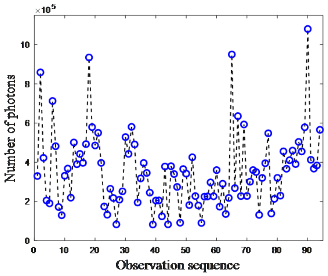
Specifically, we selected the HXMT pointed observation data with observation IDs P030229002-P030229006, corresponding to observations of the Crab pulsar from 13 September 2020 to 13 November 2020. These data were selected mainly because the observation conditions during this time interval are relatively stable, and the data quality is relatively consistent. After screening by GTI, pointing, SAA, Earth occultation, bright-Earth contamination, PI, and GRADE, these observations can still provide a sufficient number of valid photon events with relatively stable distributions. They were divided into 94 independent observation segments, which are suitable for statistical comparison among different time-delay estimation methods. It should be noted that the proposed method does not rely on specific observation IDs. These five groups of data were selected only for method performance testing and comparative analysis under relatively stable and consistent data conditions. The photon-number distribution contained in these observation events is shown in Figure 7.

4.2. Period-Estimation Performance and Ablation Analysis

First, we analyze the pulsar period estimation performance for nearly one hundred observation events in the HXMT data. We use the ${\chi }^2$-test method, the $Z^2$-test method, the period criteria in Section 2.2 (PCA-1 and PCA-2), the period criterion in Section 2.3 (SVR-1), and the proposed PCA-SVR method to carry out a comparative analyses of period estimation accuracy. Specifically, the number of bins is set to 300, and the period-search step size is set to 0.1 ns. 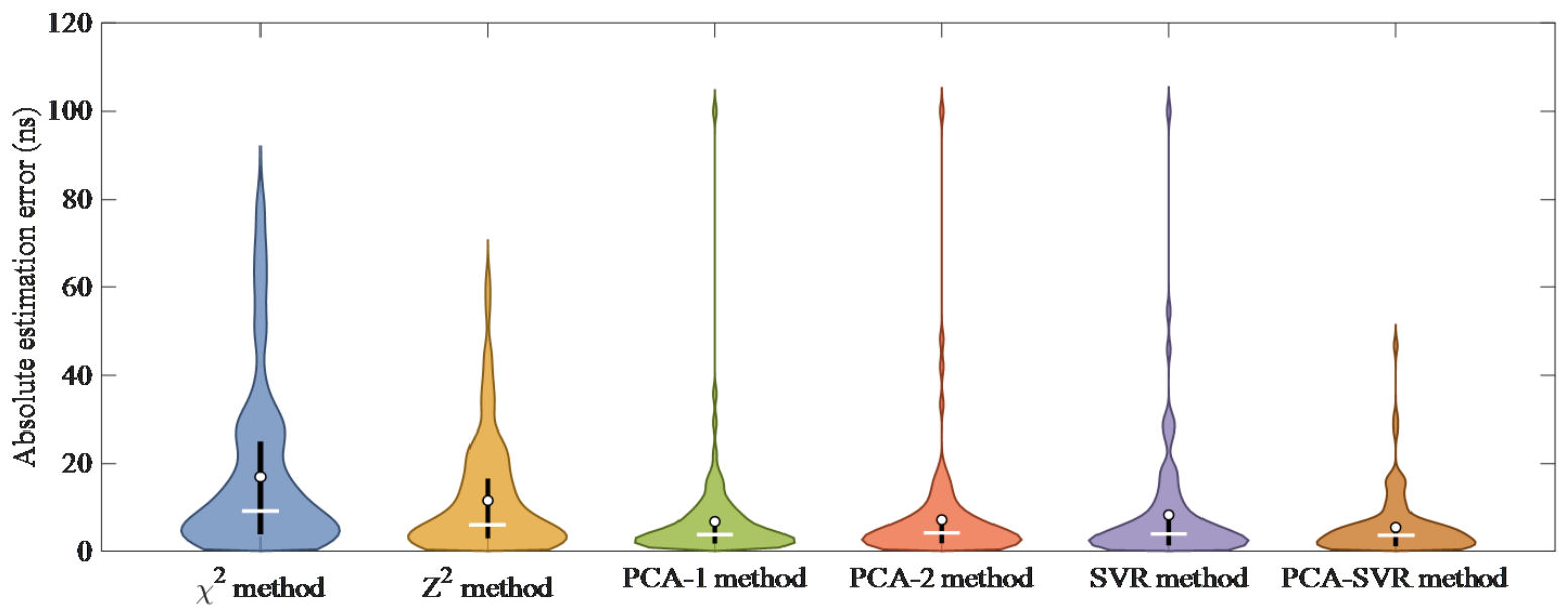Figure 8 shows the violin plots of the period estimation errors for the above six methods.

As can be seen in Figure 8, the mean estimation error of the ${\chi }^2$-test method is 16.9798 ns, the mean estimation error of the $Z^2$-test method is 11.5606 ns, the mean estimation error of the PCA-1 method is 6.7447 ns, the mean estimation error of the PCA-2 method is 7.1447 ns, the mean estimation error of the SVR-1 method is 8.2543 ns, and the mean estimation error of the PCA-SVR method is 5.4032 ns. Compared with the classical ${\chi }^2$-test method and $Z^2$-test method, the PCA-SVR method obviously exhibits higher estimation accuracy and a more stable distribution range. Compared with the three independent criteria proposed in this paper, the PCA-SVR method has a smaller interquartile range and a shorter long-tail distribution. This indicates that the proposed method can not only effectively improve period estimation accuracy but also significantly enhance the robustness of the estimation method.

To examine whether the above error differences are statistically significant, this paper uses the Wilcoxon signed-rank test [42] for paired statistical analysis. Since the six methods use the same set of HXMT observation events, the errors of different methods have a paired relationship. Meanwhile, the distribution of period-estimation errors has long-tail characteristics and is difficult to directly assume as normally distributed. Therefore, this paper adopts the nonparametric Wilcoxon signed-rank test to compare the absolute error differences between the PCA-SVR method and the other five methods. The significance level is set to 0.05, and the Holm–Bonferroni method [43] is further used for multiple-comparison correction among the five pairwise comparisons, as shown in

Table 1. Wilcoxon significance test results.

Comparison	p-Value	z-Value	Significant After Holm Correction
PCA-SVR vs. ${\chi }^2$	$1.01\times {10}^{-12}$	$-7.033$	Yes
PCA-SVR vs. $Z^2$	$2.61\times {10}^{-8}$	$-5.443$	Yes
PCA-SVR vs. PCA-1	$0.0223$	$-2.008$	Yes
PCA-SVR vs. PCA-2	$0.00448$	$-2.613$	Yes
PCA-SVR vs. SVR	$0.0162$	$-2.140$	Yes

.

As shown in Table 1, the p-values of the PCA-SVR method compared with the ${\chi }^2$, $Z^2$, PCA-1, PCA-2, and SVR-1 methods are $1.01\times {10}^{-12}$, $2.61\times {10}^{-8}$, $0.0223$, $0.00448$, and $0.0162$, respectively. After Holm–Bonferroni correction, all comparisons still satisfy the significance requirement. This indicates that, under the HXMT observation data conditions tested in this paper, the PCA-SVR method achieves statistically significant reductions in period-estimation error compared with the traditional methods and the single-criterion methods.

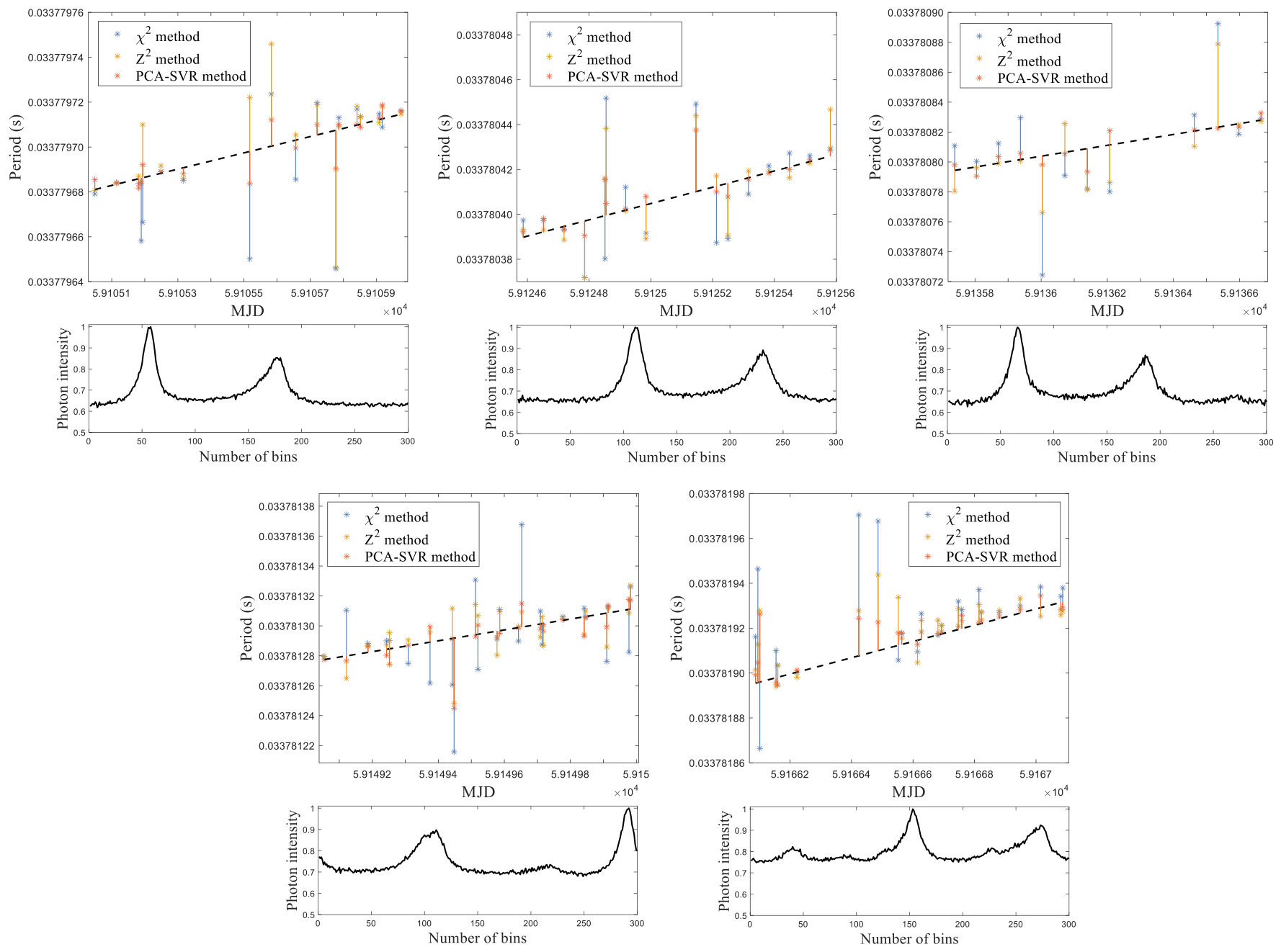
Figure 9 shows the distribution of the results obtained after period estimation for these independent observation events by the ${\chi }^2$-test method, the $Z^2$-test method, and the PCA-SVR method (with the contemporaneous period observation results released by the Jodrell Bank Observatory in the UK taken as the reference).

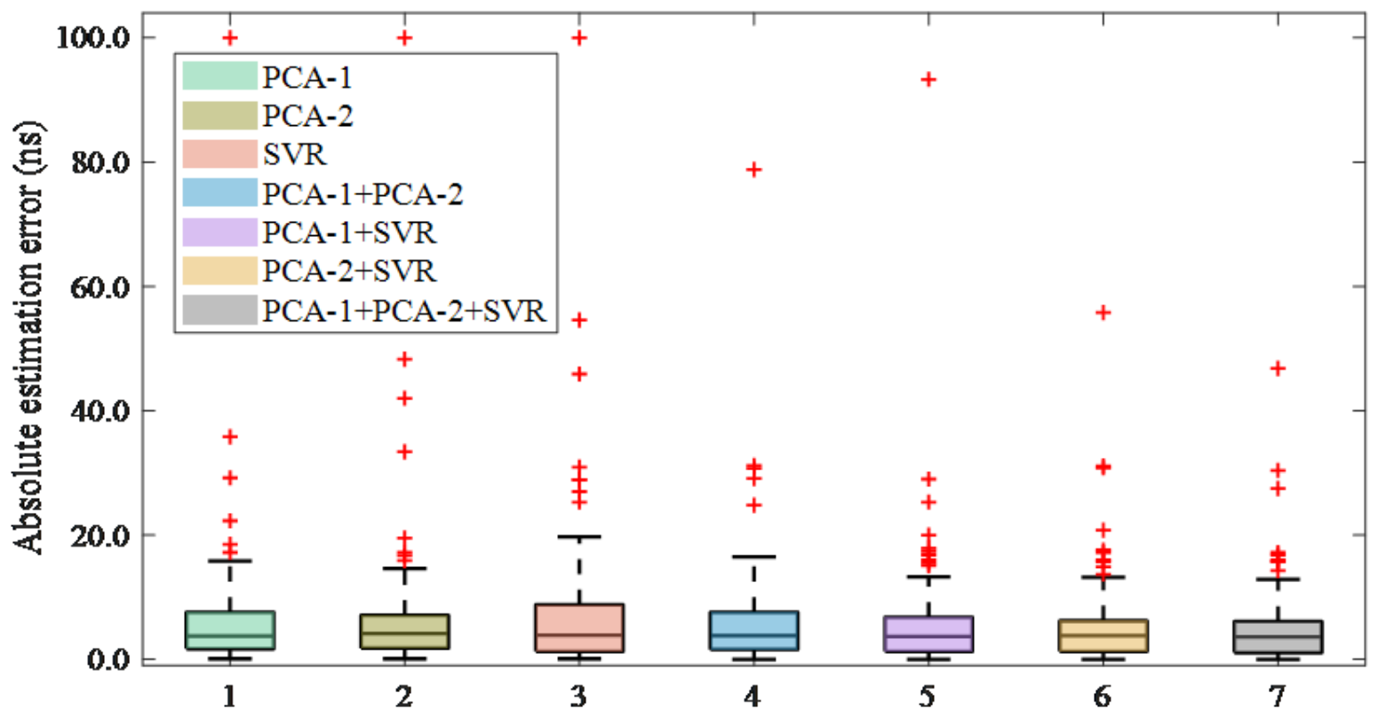
Next, we further conducted an ablation test for the three period criteria proposed in this paper. Figure 10 shows the box plots of the period-estimation errors obtained from the HXMT observation data under different combinations of the three period criteria.

As can be seen from Figure 10, the period estimation errors of the three period criteria under the seven combination strategies are 6.7447 ns, 7.1447 ns, 8.2543 ns, 6.5755 ns, 6.1574 ns, 5.8601 ns, and 5.4032 ns, respectively. When all three period criteria are included in the test, the period estimation accuracy is the highest, and the distribution range of outliers is the smallest. This indicates that the proposed PCA-SVR method can indeed achieve better estimation accuracy and stability.

4.3. Time-Delay Estimation Performance

Based on the above period estimation results and combined with Section 2.4, we further conduct a comparative analysis of the estimation performance for pulsar measurement information (time-delay).

Table 2. Comparison of time-delay estimation performance of the three methods.

Method	Mean Time-Delay Estimation Error (μs)	STD of Time-Delay Estimation Error (μs)	95% Confidence Interval (μs)
${\chi }^2$ method	79.1619	74.1951	[63.9652, 94.3585]
$Z^2$ method	50.0194	62.2565	[37.2680, 62.7707]
PCA-SVR method	24.7942	25.4538	[19.5808, 30.0076]

presents a comparison of the mean error, standard deviation, and 95% confidence interval of the time-delay estimation results obtained by the ${\chi }^2$-test method, the $Z^2$-test method, and the PCA-SVR method using nearly one hundred sets of HXMT satellite observation data.

As can be seen in Table 2, compared with the ${\chi }^2$-test method and the $Z^2$-test method, the PCA-SVR method improves the time-delay estimation accuracy by 68.68% and 50.43%, respectively, and improves the estimation stability by 65.69% and 59.11%, respectively. This indicates that the PCA-SVR method can achieve higher estimation accuracy and stronger estimation stability in pulsar time-delay estimation.

In summary, the test results based on the on-orbit observation data from the Insight-HXMT satellite show that, compared with the existing benchmark methods, the PCA-SVR method proposed exhibits superior performance in pulsar time-delay estimation and can provide measurement information with higher accuracy and higher reliability for subsequent pulsar navigation tests.

5. Multi-Scenario Pulsar Navigation Simulation and Performance Evaluation

In this section, the PCA-SVR method is applied to typical pulsar navigation mission scenarios such as the Earth-orbiting phase, the Earth-Moon transfer phase, and the Mars approach phase. Through navigation and positioning simulation analysis, the applicability, stability, and robustness of the PCA-SVR method under different orbital scales and different observation geometry conditions are quantitatively discussed.

5.1. Simulation Settings and Parameter Rationale

In this paper, the simulation parameters are set according to the orbital scale, the time scale of dynamical variation, the pulsar observation accumulation requirement, and the measurement-update frequency in each mission phase. In the near-Earth orbit phase, the orbital period is short, and the state changes relatively fast, so a shorter orbit-propagation step size and measurement-update interval are adopted. In the Earth-Moon transfer phase, the orbital scale increases and the probe state changes more slowly, so the simulation step size and measurement-update period are properly extended. The Mars approach phase belongs to an interplanetary flight scenario, in which the navigation arc and the time scale of dynamical evolution further increase. Therefore, a longer simulation step size and filtering-update interval are adopted. Meanwhile, to ensure consistent comparison among different time-delay estimation methods in the navigation simulations, the detector effective area, background flux, pulsar observation modeling method, filtering framework, and Monte Carlo simulation number are kept the same for all methods. The main simulation parameters of each scenario are listed in

Table 3. Main simulation parameter settings for different scenarios.

Parameter	Earth-Orbiting Phase	Earth–Moon Transfer Phase	Mars Approach Phase
Simulation duration	86,400 s	172,800 s	1,296,000 s
Orbit propagation step size	3 s	5 s	1200 s
Measurement update interval	150 s	600 s	1200 s
Single observation duration	100 s	600 s	1000 s
Effective detector area	1000 cm2	1000 cm2	1000 cm2
Background noise flux	0.005 ph/cm2/s	0.005 ph/cm2/s	0.005 ph/cm2/s
Number of Monte Carlo simulations	100	100	100

.

5.2. Scenario 1: Earth-Orbiting Phase

To ensure the accuracy of the orbit propagation results, this paper uses an HPOP (high-precision orbit propagator) to perform orbit simulation for the target satellite. The satellite state is given in the form of classical orbital elements and is defined in the International Celestial Reference Frame (ICRF). The orbital epoch is set to 16 January 2026 04:00:00.000 UTCG, and the coordinate epoch is set to J2000.0. The initial orbital elements of the satellite are set as follows: The semi-major axis is 6798.14 km, the eccentricity is 0.0005, the orbital inclination is 51.6°, the right ascension of the ascending node is 0°, the argument of perigee is 0°, and the true anomaly is 0°. Considering the duration requirement for pulsar data accumulation, this paper adopts an asynchronous UKF strategy. The state is propagated recursively with a step size of 3 s, and the measurements are updated with a period of 150 s. Only time updating is performed within the measurement interval, and correction is executed when measurements arrive. The process noise covariance matrix is set as follows:

$$\mathbf{Q}=diag{\left[q,q,q,q\times {10}^{-3},q\times {10}^{-3},q\times {10}^{-3}\right]}^T$$

where $q=0.1$.

The initial filtering error is set as follows:

$$d\mathbf{X}={\left[1000,1000,1000,1,1,1\right]}^T$$

The initial covariance matrix is set as follows:

$$\mathbf{P}\left(0\right)=diag\left(d\mathbf{X}\right)·diag\left(d\mathbf{X}\right)$$

The above parameters are used to characterize the initial uncertainty of the filtering process and the equivalent model error during state propagation. Their values are mainly set according to the orbital scale and filtering stability requirements of each scenario.

First, this section adopts a pure pulsar navigation scheme using PSR J0534+2200, PSR J1952+3252, and PSR J0659+1414 as the target navigation sources. According to Ref. [2], we simulated the pulsar photon sequences received by the probe. In each filtering step, the specific parameter settings are shown in Table 3. The PCA-SVR method and the ${\chi }^2$-test method in Section 4 were used to perform Monte Carlo simulations of the pulsar time-delay information, and the resulting estimates were taken as measurement information and input into the navigation simulation system so as to realize pulsar navigation simulation under a complete chain from photon-data simulation to final navigation filtering.

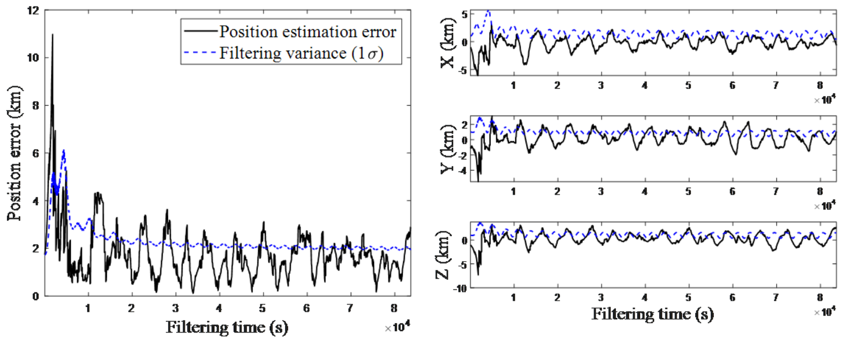
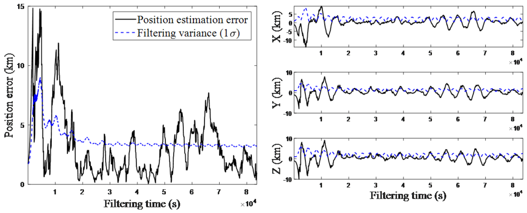
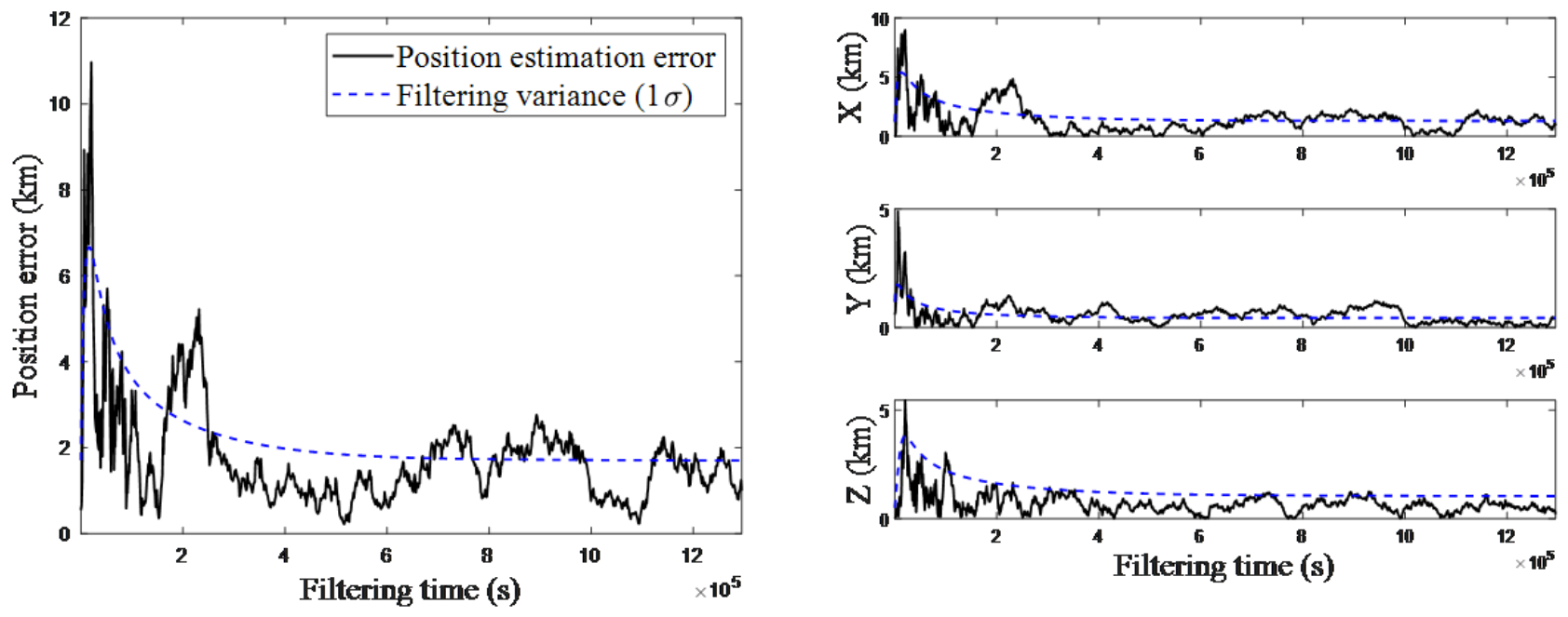
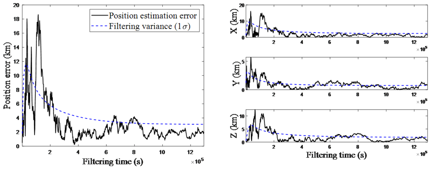
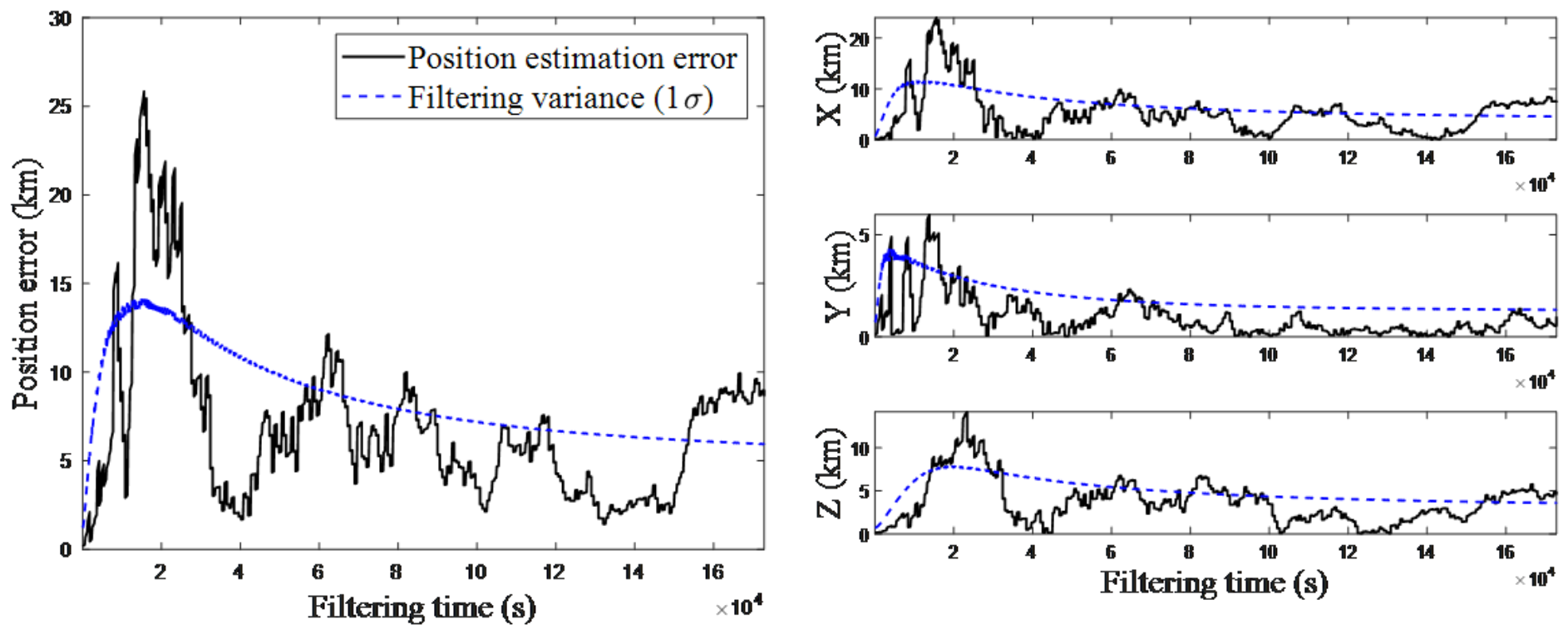
Figure 11 and Figure 12 present the pulsar navigation filtering processes under the two time-delay estimation methods. In this process, the standard deviations of the time-delay information calculated by the PCA-SVR method and the ${\chi }^2$-test method are $2.9581\times {10}^{-5}$ s and $6.1438\times {10}^{-5}$ s, respectively. We performed Monte Carlo simulations for the above process. The results show that, under the PCA-SVR method, the mean navigation position error is 1735.5443 m, the mean RMS of the position error is 1959.4860 m, the mean velocity error is 1.8862 m/s, and the mean RMS of the velocity error is 2.1272 m/s. Under the ${\chi }^2$-test method, the mean navigation position error is 2439.1460 m, the mean RMS of the position error is 2794.4568 m, the mean velocity error is 2.6405 m/s, and the mean RMS of the velocity error is 3.0005 m/s. Compared with the ${\chi }^2$-test method, the mean RMS of the navigation position error under the PCA-SVR method is improved by 834.9708 m. This indicates that the improvement of time-delay estimation accuracy by the PCA-SVR method can be clearly reflected in the final navigation and positioning results.

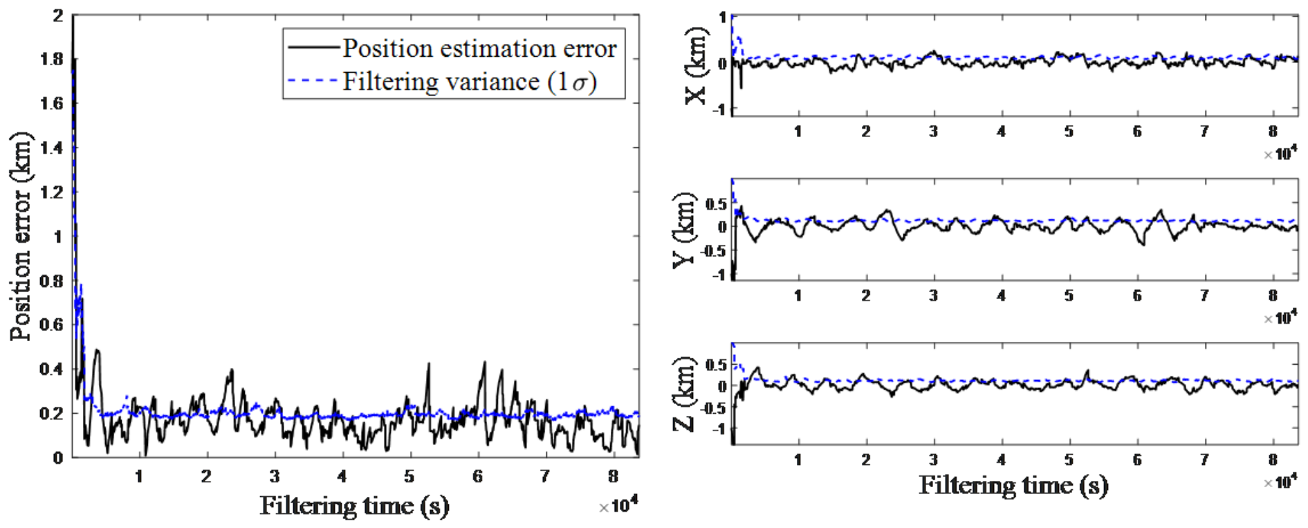
Next, in the Earth satellite scenario, although the PCA-SVR method significantly improves the navigation and positioning performance, there is still a certain gap from the requirement of high-precision Earth satellite navigation and positioning. Therefore, this subsection further discusses starlight-refraction/pulsar combined navigation. Specifically, we still use the PCA-SVR method to estimate pulsar time-delay, and we combine one starlight refraction source with one pulsar source for joint measurement information observation. The starlight-refraction measurement noise is set to 100 m, while the other parameter settings remain the same as above.

Figure 13 shows the filtering process of the starlight-refraction/pulsar combined navigation. We also performed Monte Carlo simulations for the above process. The results show that the mean navigation position error is 182.3664 m, the mean RMS of the position error is 203.1654 m, the mean velocity error is 0.2093 m/s, and the mean RMS of the velocity error is 0.2350 m/s. It can be seen that, after fusing pulsar navigation based on high-accuracy pulsar time-delay estimation with starlight-refraction navigation, the positioning accuracy of the combined navigation is significantly improved and can satisfy the Earth satellite navigation and positioning requirements.

5.3. Scenario 2: Earth-Moon Transfer Phase

This subsection mainly takes the Earth-Moon probe as the target to simulate the navigation filtering process in the Earth-Moon transfer phase. We adopt a method based on B-Plane parameter constraints to accomplish Earth-Moon trajectory design. The launch time is set to 31 December 2024 13:40:49.858 UTCG, and the mission end time is set to 4 January 2025 11:59:59.975 UTCG. Among them, the orbital window from 1 January 2025 12:00:00.000 UTCG to 3 January 2025 12:00:00.000 UTCG is selected as the Earth-Moon transfer phase. This subsection also adopts an asynchronous UKF strategy. The process noise covariance matrix is set as follows:

$$\mathbf{Q}=diag{\left[q_1,q_1,q_1,q_2(3e-1),q_2(3e-1),q_2(3e-1)\right]}^T$$

where $q_1=2\times {10}^{-12}$ and $q_2=5\times {10}^{-7}$.

The initial filtering error is set as follows:

$$d\mathbf{X}={\left[100,100,100,0.1,0.1,0.1\right]}^T$$

The initial covariance matrix is set as follows:

$$\mathbf{P}=diag{\left[p,p,p,p\times {10}^{-5},p\times {10}^{-5},p\times {10}^{-6}\right]}^T$$

where $p=5\times {10}^5$.

This subsection likewise adopts a pure pulsar navigation scheme, using PSR J0534+2200, PSR J1952+3252, and PSR J0659+1414 as the target navigation sources. The PCA-SVR method and the ${\chi }^2$-test method in Section 4 are used to perform Monte Carlo simulations of the pulsar time-delay information, and the resulting estimates are taken as measurement information and input into the navigation simulation system.

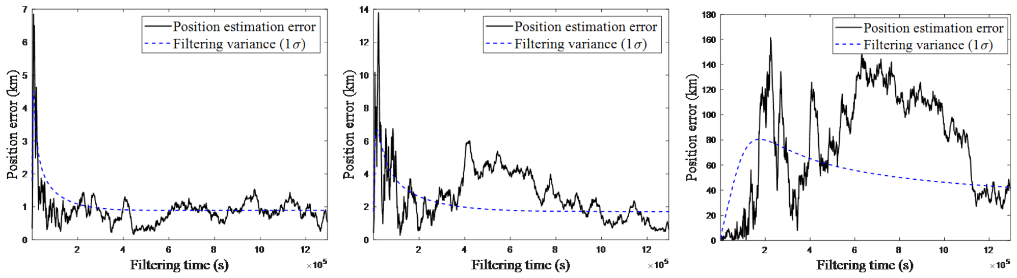
Figure 14 and Figure 15 present the pulsar navigation filtering processes under the two time-delay estimation methods, respectively. In this process, the standard deviations of the time-delay information calculated by the PCA-SVR method and the ${\chi }^2$-test method are $1.1710\times {10}^{-5}$ s and $2.7435\times {10}^{-5}$ s, respectively. We performed Monte Carlo simulations for the above process. The results show that, under the PCA-SVR method, the mean navigation position error is 2191.5300 m, the mean RMS of the position error is 2384.9001 m, the mean velocity error is 0.0280 m/s, and the mean RMS of the velocity error is 0.0301 m/s. Under the ${\chi }^2$-test method, the mean navigation position error is 5012.4662 m, the mean RMS of the position error is 5427.4618 m, the mean velocity error is 0.0466 m/s, and the mean RMS of the velocity error is 0.0509 m/s. In the Earth–Moon transfer phase, navigation and positioning accuracies under the ${\chi }^2$-test method decrease significantly. The main reason is that the measurement noise corresponding to this method is relatively large, and this paper adopts an asynchronous filtering strategy. Under the condition that only a 2-day simulation window is set in the Earth-Moon transfer phase, the filter convergence process is limited, making it difficult to enter a stable stage, which in turn leads to poor navigation accuracy. In contrast, the PCA-SVR method has a faster filter convergence rate, and its mean RMS of the navigation position error is improved by 3042.5617 m compared with the ${\chi }^2$-test method.

5.4. Scenario 3: Mars Approach Phase

This subsection mainly takes the Mars probe as the target to simulate the deep-space navigation filtering process in the Mars approach phase. We adopt an Earth-Mars transfer trajectory design based on the asymptotic velocity vector. The orbital elements at launch from Earth are listed in

Table 4. Orbital element settings based on the asymptotic velocity vector.

Parameters	Value
Radius of Periapsis	6678 km
C3 Energy	13.2035 km2/s2
RA of Outgoing Asymptote	25.2785 deg
Declination of Outgoing Asymptote	0.0483 deg
Velocity Azimuth at Periapsis	0 deg
True Anomaly	0 deg

.

The start time of the trajectory design is 17 July 2020 00:00:00.000 UTCG, and the spacecraft begins to enter the Mars-orbiting phase at 3 January 2021 00:00:00.004 UTCG. Therefore, this subsection selects the orbital window from 1 December 2020 00:00:00.000 UTCG to 15 December 2020 00:00:00.000 UTCG as the Mars approach phase. The coordinate epoch is set to J2000.0. The process noise covariance matrix is set as follows:

$$\mathbf{Q}=diag{\left[q_1,q_1,q_1,q_2(3e-1),q_2(3e-1),q_2(3e-1)\right]}^T$$

where $q_1=2\times {10}^{-12}$ and $q_2=5\times {10}^{-7}$.

The initial filtering error is set as follows:

$$d\mathbf{X}={\left[100,100,100,0.001,0.001,0.001\right]}^T$$

The initial covariance matrix is set as follows:

$$\mathbf{P}=diag{\left[p,p,p,p\times {10}^{-5},p\times {10}^{-5},p\times {10}^{-6}\right]}^T$$

where $p=1\times {10}^5$.

This subsection likewise adopts a pure pulsar navigation scheme using PSR J0534+2200, PSR J1952+3252, and PSR J0659+1414 as the target navigation sources. The PCA-SVR method and the ${\chi }^2$-test method in Section 4 are used to perform Monte Carlo simulations of the pulsar time-delay information, and the resulting estimates are taken as measurement information and input into the navigation simulation system. 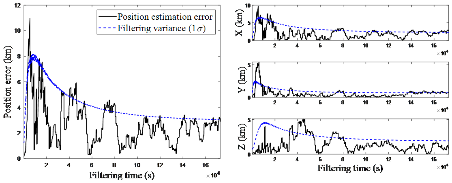Figure 16 and Figure 17 present the pulsar navigation filtering processes under the two time-delay estimation methods. In this process, the standard deviations of the time-delay information calculated by the PCA-SVR method and the ${\chi }^2$-test method are $1.0187\times {10}^{-5}$ s and $2.2406\times {10}^{-5}$ s, respectively.

We performed Monte Carlo simulations for the above process, and

Table 5. Navigation results of the two estimation methods during the Mars approach phase.

Method	Position Error (m)	Position Error RMS (m)	Velocity Error (m/s)	Velocity Error RMS (m/s)
${\chi }^2$ method	2513.9613	2749.3205	0.0158	0.0163
PCA-SVR method	1570.2450	1703.2697	0.0118	0.0123

gives the navigation filtering results under the two estimation methods. It can be seen that, compared with the ${\chi }^2$-test method, the mean RMS of the navigation position error under the PCA-SVR method is improved by 1046.0508 m.

In summary, through full-chain simulation validation of typical pulsar navigation mission scenarios such as the Earth-orbiting phase, the Earth-Moon transfer phase, and the Mars approach phase, it can be seen that the PCA-SVR-based pulsar time-delay estimation method proposed can not only effectively reduce measurement errors but also significantly improve the accuracy of navigation filtering results, thereby enhancing pulsar navigation and positioning performance. Meanwhile, comparative results across multiple scenarios further indicate that, under limited detector area, pulsar navigation shows greater potential for long-duration autonomous deep-space remote sensing and navigation missions, where observation time can be accumulated more sufficiently.

6. Discussions

6.1. Methodological Implications of the Waterfall-Plot Multi-Criteria Framework

The waterfall-plot multi-criteria framework proposed extends pulsar period discrimination from traditional single folded-profile significance analysis to two-dimensional structural analysis of segmented folded profiles. The waterfall plot preserves both phase-dimensional and time-segment-dimensional information, and it can therefore describe the concentration, projection response, and phase-drift characteristics of the pulse profile under a candidate period.

Among the three criteria, the PCA-based structural significance criterion reflects the concentration degree of the dominant structure, the principal-projection significance criterion characterizes the response strength along the principal-component direction, and the SVR-based peak-trajectory consistency criterion describes the geometric drift of the same physical peak in segmented profiles. These three criteria evaluate the candidate period from the complementary perspectives of structure, projection, and geometry. As a result, period estimation no longer relies on a single statistical quantity, and the adaptability of the method to local noise and profile fluctuations is improved.

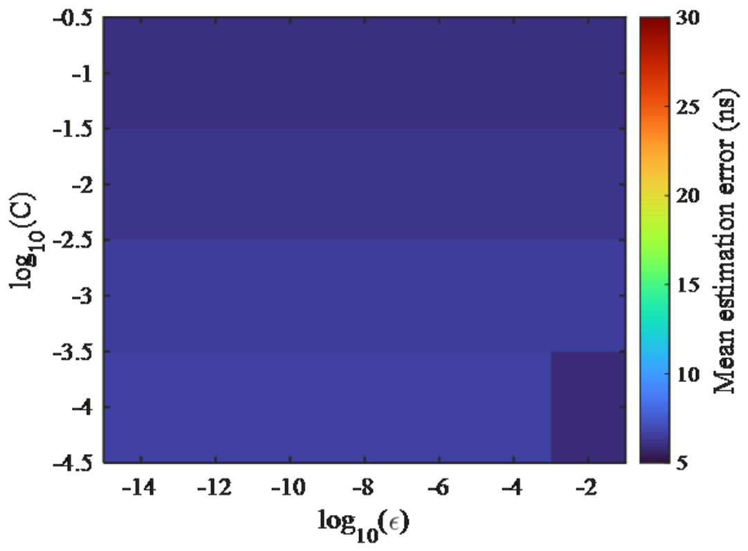
6.2. Sensitivity Analysis of SVR Hyperparameters

To analyze the influence of SVR hyperparameters on peak-trajectory slope estimation and period-estimation results, this paper further conducts a hyperparameter sensitivity analysis for the penalty coefficient C and the insensitive loss function $ϵ$. The penalty coefficient C is set to 0.0001, 0.001, 0.01, and 0.1, and the insensitive loss function $ϵ$ is set to ${10}^{-14}$, ${10}^{-12}$, ${10}^{-10}$, ${10}^{-8}$, ${10}^{-6}$, ${10}^{-4}$, and ${10}^{-2}$. A grid search is then performed over these parameter combinations. The observation duration is set to 200 s, and the remaining simulation parameters are consistent with those in Section 5. Figure 18 shows the statistical mean period-estimation errors obtained from Monte Carlo simulations using the SVR single-period criterion under different hyperparameter combinations.

In the analyses in Section 4 and Section 5, the penalty coefficient C is set to 0.001, and the insensitive loss function $ϵ$ is set to ${10}^{-10}$. As can be seen in Figure 18, within the tested parameter range, the overall variation in error is small, and the mean error remains at a similar level, indicating that the SVR criterion is not strongly sensitive to hyperparameter changes. Relatively, an excessively small penalty coefficient C may weaken the response of the model to the peak-drift trend, while a moderate parameter combination can achieve a better balance between suppressing local noise and maintaining slope sensitivity.

6.3. Robustness Under High-Background and Weak-Source Conditions

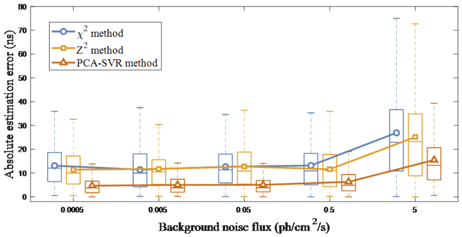
This section mainly discusses the robustness and generalization performance of the PCA-SVR method. First, to investigate the robustness of the proposed method, we discuss the influence of the background noise flux of the Crab pulsar. The background noise flux is set to 0.0005 ph/cm²/s, 0.005 ph/cm²/s, 0.05 ph/cm²/s, 0.5 ph/cm²/s, and 5 ph/cm²/s, while the remaining simulation parameters are consistent with those in Section 6.2. Figure 19 shows the statistical distributions of the period estimation errors obtained by Monte Carlo simulations under different background noise fluxes using the PCA-SVR method, the ${\chi }^2$ test method, and the $Z^2$ test method.

It can be seen from Figure 19 that, as the background noise increases, the mean estimation errors of all three methods show an increasing trend. However, the statistical mean error of the PCA-SVR method is always smaller than those of the other two methods. This indicates that the proposed method can maintain a better estimation level under different background noise intensities. Meanwhile, compared with the other two methods, the PCA-SVR method shows a smaller interquartile range in repeated Monte Carlo simulations. This means that the proposed method also has better estimation stability under different background noise intensities.

Next, to investigate the generalization performance of the proposed method, we further selected PSR B1509-58, which has a simpler profile and a weaker flux, and we used the above three methods to test the period estimation performance. Compared with the Crab pulsar, PSR B1509-58 shows a simpler single-peak profile, with an effective flux of only 0.0162 ph/cm²/s and a pulsed fraction of 0.646. According to the true-period variation, the simulation period is fixed at 0.1507 s, the background noise flux is set to 0.005 ph/cm²/s, and the search step size is set to 0.1 μs. 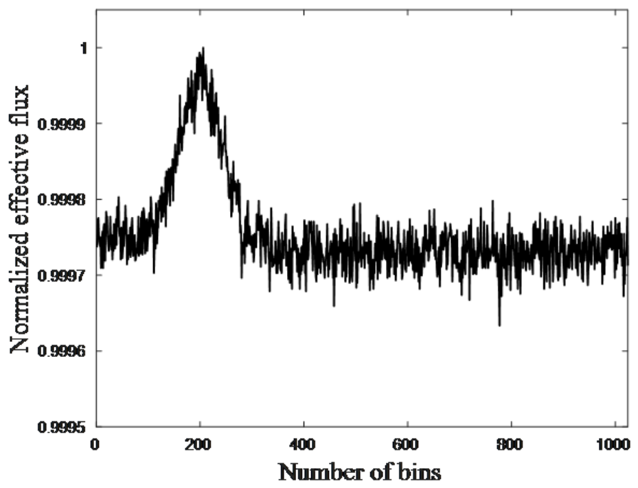Figure 20 shows the true profile of PSR B1509-58 [44].

Table 6. Mean errors, standard deviations, and 95% confidence intervals of period estimation for the three methods.

Method	Mean Period Estimation Error (μs)	STD of Period Estimation Error (μs)	95% Confidence Interval (μs)
${\chi }^2$ method	1.8160	1.3105	[1.5591, 2.0729]
$Z^2$ method	0.9280	0.8305	[0.7652, 1.0908]
PCA-SVR method	0.8660	0.6920	[0.7304, 1.0016]

presents the statistical mean, standard deviation, and 95% confidence interval of the period estimation errors of the three methods obtained from Monte Carlo simulations.

As can be seen from Figure 20 and Table 6, the effective flux of PSR B1509-58 is significantly lower than that of the Crab pulsar, and therefore, the estimation accuracy of all three methods decreases accordingly. However, the PCA-SVR method still has the smallest mean estimation error and standard deviation. This indicates that the proposed method is not only suitable for the Crab pulsar with significant flux but also has considerable potential for high-quality navigation pulsars with relatively weak flux characteristics.

6.4. Influence of Pulsar Source and Configuration on Navigation Performance

In the above navigation simulations, three fixed pulsar sources are used to ensure that different time-delay estimation methods are compared under the same observation conditions. However, pulsar navigation performance is affected not only by the time-delay estimation accuracy of individual pulsars but also by the directional distribution of the selected pulsars. Different pulsar configurations change the geometric constraint relationship between the measurements and the spacecraft position state, thereby affecting the amplification degree from time-delay errors to position errors. Therefore, we further analyze the influence of pulsar configurations on navigation geometry performance.

Six candidate navigation pulsars are selected: J0659+1414, J0218+4232, J0437-4715, J1952+3252, J0534+2200, and J1939+2134. All three-pulsar combination schemes are enumerated, and the PDOP-like geometric factor, minimum angular separation, and volume index are calculated. Among them, the PDOP-like factor is used to describe the amplification effect of the observation geometry on the three-dimensional position error, while the minimum angular separation and the volume index respectively reflect the directional dispersion of the pulsars and the three-dimensional geometric span capability. The PDOP-like geometric factor is specifically expressed as

$$\mathit{n}={[cos\delta cos\alpha ,cos\delta sin\alpha ,sin\delta ]}^T$$

(26)

$$H=[{\mathit{n}}_1^T;{\mathit{n}}_2^T;{\mathit{n}}_3^T]$$

(27)

$$PDOP-like=\sqrt{\mathrm{tr}\left({\left(H^{T}H\right)}^{+}\right)}$$

(28)

where $\delta$ and $\alpha$ are the declination and right ascension of the pulsar, respectively. $\mathit{n}$ is the unit direction vector of the pulsar. H is the line-of-sight direction matrix formed by the three pulsars. $PDOP-like$ is the position-dilution-of-precision-like factor, which is used to describe the amplification effect of the pulsar-direction geometry on the position error.

Table 7. Comparison results of the indicators for three typical combination schemes.

Combination Scheme	PDOP-Like Geometric Factor	Minimum Angular Separation	Volume Index
J0659+1414/J0218+4232/J0437-4715	1.996	66.077	0.824
J1952+3252/J0659+1414/J0534+2200	5.690	21.676	0.216
J1952+3252/J0659+1414/J1939+2134	214.516	11.675	0.005

gives the comparison results of the indicators for three typical combination schemes. The PDOP-like geometric factors correspond to the optimal, moderate, and poor configurations, respectively. It can be seen from the table that the geometric indicators of different three-pulsar combinations are significantly different. The optimal configuration has a smaller PDOP-like geometric factor and a larger volume index, indicating that the directions of the three pulsars are more dispersed and can form more stable three-dimensional geometric constraints. The baseline configuration used in the original navigation simulation, namely J1952+3252/J0659+1414/J0534+2200, has a relatively small PDOP-like geometric factor, and it has a larger minimum angular separation and volume index. Therefore, it can also complete the navigation solution. However, the PDOP-like geometric factor of the poor configuration increases significantly, and the volume index is close to zero, indicating that the directional geometry of the three pulsars is poor and the measurement errors are more likely to be amplified in the position solution.

Figure 21 shows the navigation positioning filtering results obtained using the above three pulsar configurations in the Mars approach simulation. Combination scheme 2 is the pulsar configuration adopted in Section 5.4. It can be seen that the positioning error of combination scheme 1 is smaller than that of combination scheme 2, which is approximately 1.5 km. However, when combination scheme 3 is used, the positioning error is relatively large, indicating that pulsar navigation may not be feasible under this configuration.

6.5. Interpretation of Simulation-Based Navigation Improvements

The validation process in this paper includes two aspects. First, actual observation data from the Insight-HXMT satellite are used to verify the performance of the PCA-SVR method in pulsar period estimation and time-delay estimation. Second, navigation simulations are carried out under preset dynamical models, measurement models, filtering strategies, and pulsar-source configurations. Therefore, the navigation simulation results mainly reflect the propagation effect of time-delay estimation errors on the final navigation solution.

Under the same simulation conditions, the proposed method reduces the pulsar time-delay estimation error and further improves the positioning performance in scenarios such as near-Earth orbit, Earth-Moon transfer, and Mars approach. The above results show that, within the multi-scenario simulation framework set in this paper, improving the accuracy of pulsar time-delay estimation can effectively improve pulsar-navigation filtering performance and provide a reference for the optimization of measurement-information acquisition methods in future navigation applications.

6.6. Other Error Sources and Their Effects

In addition to time-delay estimation errors, practical pulsar navigation performance is also jointly affected by multiple error sources. First, pulsar direction errors affect the line-of-sight direction vector in the measurement model, causing deviations in the projection relationship between the spacecraft position and the pulsar direction. Second, ephemeris errors affect the position calculation of the Sun, Earth, Moon, or planets, and they further affect time-delay corrections, dynamical propagation, and reference-frame transformation processes. Detector timing errors directly act on photon time-of-arrival tags, thereby affecting profile folding, phase estimation, and time-delay estimation results.

In addition, spacecraft clock errors introduce common bias or slow drift into the observed pulsar arrival times, which need to be modeled or calibrated in the navigation solution. Attitude errors affect the detector pointing and effective collecting area, thereby changing the count rate, background noise level, and reconstructed profile quality. Dynamical modeling errors mainly arise from inaccurate force-model parameters, unmodeled perturbations, and orbit-propagation errors, and they affect the state prediction accuracy of the filter during the measurement-update interval.

Therefore, the navigation simulations in this paper are mainly used to analyze the influence of improved pulsar time-delay estimation accuracy on the navigation filtering results. In the simulation framework set in this paper, part of the system errors, observation noise, and unmodeled perturbations are represented by the lumped error terms in the measurement model and state model. Future work can further combine specific mission scenarios to carry out more detailed error modeling, sensitivity analysis, and integrated error-budget evaluation for the above error sources.

7. Conclusions

This paper proposed a pulsar time-delay estimation method based on a waterfall-plot multi-criteria framework and conducted full-chain pulsar navigation simulation and performance evaluation for typical mission scenarios such as the Earth-orbiting phase, the Earth-Moon transfer phase, and the Mars approach phase. The main conclusions are as follows.

1. Accuracy Improvement in Pulsar Time-Delay Estimation: By constructing a pulsar profile waterfall-plot model, the proposed method extracts period-structure features from the perspectives of principal eigenvalue contribution, principal-projection significance, and geometric consistency of the peak trajectory, thereby achieving accurate period prediction and further improving the estimation accuracy of pulsar time-delay information. Combined with HXMT satellite observation data, the time-delay estimation error of the proposed method is 24.7942 μs. Compared with the ${\chi }^2$-test method and the $Z^2$-test method, the estimation accuracy is improved by 68.68% and 50.43%, respectively.

2. Stability Enhancement in Pulsar Time-Delay Estimation: The proposed method constructs a time-delay estimation method based on a waterfall-plot multi-criteria framework according to different evaluation criteria. Among them, the multi-criteria fusion strategy further improves the robustness of pulsar time-delay estimation. Based on HXMT satellite observation data, compared with the ${\chi }^2$-test method and the $Z^2$-test method, the stability of the proposed method is improved by 65.69% and 59.11%, respectively.

3. Navigation Positioning Performance Gains: A full-chain simulation framework was constructed, covering the entire process from detector event-data simulation to final navigation and positioning filtering, and the practical improvement of the proposed method on final navigation performance was verified. Under the adopted simulation settings, the proposed method leads to positioning accuracy improvements of approximately 0.83 km, 3.04 km, and 1.05 km over the ${\chi }^2$-test method in the Earth-orbiting, Earth-Moon transfer, and Mars approach phases, respectively.

In summary, the waterfall-plot multi-criteria method proposed can improve pulsar period and time-delay estimation from three complementary aspects: structural significance, projection response, and geometric consistency. It provides an interpretable analysis framework for improving pulsar time-delay acquisition. Future work can further combine weak-source observations, high-background conditions, pulsar configuration optimization, and comprehensive error modeling to systematically evaluate the applicability of the proposed method in complex pulsar navigation scenarios.