Article

Decade-Long Photometric Observations of Light Pollution and Cloud Effects on Night Sky Brightness in Hong Kong

1
Department of Physics, The University of Hong Kong, Pokfulam, Hong Kong, China
2
Spatial Sciences Institute, Dornsife College of Letters, Arts and Sciences, University of Southern California, Los Angeles, CA 90089, USA
*
Author to whom correspondence should be addressed.
This work was primarily done at the University of Hong Kong. S.L. is currently affiliated with the University of Southern California.
Remote Sens. 2026, 18(11), 1691; https://doi.org/10.3390/rs18111691
Submission received: 7 March 2026 / Revised: 25 April 2026 / Accepted: 12 May 2026 / Published: 23 May 2026
(This article belongs to the Section Atmospheric Remote Sensing)

Highlights

What are the main findings?
  • Hong Kong’s night skies are severely light-polluted, with urban areas averaging over 100 times the brightness of the international dark sky standard. Skies are brighter in the early evening than after midnight, with urban areas showing a sharper post-midnight drop.
  • The study confirms that clouds drastically amplify urban sky brightness by reflecting artificial light back to the ground, using infrared sky temperature as a quantitative indicator of cloud amount.
What are the implications of the main finding?
  • Leveraging a decade of continuous ground-based photometric data, this study provides empirical evidence linking urbanization to light pollution, affirming the critical importance of in situ observations for complementing satellite-based assessments.
  • The strong link between cloud amount and increased brightness demonstrates that light pollution degrades the nocturnal environment even on cloudy nights. The greater post-midnight dimming in cities further indicates improved compliance with lighting regulations, with positive implications for urban ecology and human health.

Abstract

This study examines how night sky brightness (NSB) in Hong Kong has evolved over the past decade. It combines recent datasets covering 2019–2023 with the earlier dataset analyzed in a previous study (2010–2013). This study emphasizes the importance of long-term monitoring in the context of light pollution variations resulting from urban development and increasing public awareness. Photometric data were collected nightly and continuously from multiple locations equipped with a Sky Quality Meter, covering both urban and suburban settings. The in situ observation frequency was at sub-minute intervals, characterizing nighttime profiles with a temporal resolution that other monitoring systems (e.g., satellites) cannot provide. Analysis reveals that Hong Kong’s night skies are substantially brighter than the International Astronomical Union’s (IAU) dark sky standard, with urban areas exceeding 100× the standard brightness on average. By comparing early- and late-night observations, we establish a robust indicator for assessing the direct impact of light pollution, concluding that early evening skies are brighter than late-night skies due to the variation in artificial lighting. Urban regions demonstrated more pronounced post-midnight darkening, a trend consistent with increased light pollution awareness and enhanced compliance with late-night lighting protocols. Additionally, this study introduces remotely sensed infrared (IR) sky temperature as a novel cloud amount indicator, demonstrating a strong positive correlation between cloud amount and NSB, particularly in urban areas. Our findings highlight the urgent need for effective light pollution mitigation strategies in rapidly developing cities like Hong Kong, offering valuable insights for similar initiatives worldwide.

1. Introduction

Light pollution is a type of environmental degradation caused by excessive artificial light at night (ALAN), which disrupts natural ecosystems [1,2,3,4,5] and obscures our night sky [6,7,8]. Light pollution has been associated with health risks and negatively affects overall quality of life [2,9,10,11]. Recognized as one of the fastest-growing forms of environmental degradation, recent studies indicate that both the total surface area of the planet exposed to light pollution and the brightness of ALAN have increased significantly in recent years [12,13]. Recognizing the importance of darkness for both urban and natural environments highlights the urgent need to monitor and manage light pollution [13,14].
One popular method for monitoring light pollution is to measure night sky brightness (NSB) using semiconductor photometers at specific locations [15,16,17,18]. These photometers [19], including the Sky Quality Meter (SQM) [20] and the Photometer–Telescope Encoder and Sky Sensor (TESS-W) [21], are accurate and cost-effective, have high sampling rates, and are easy to install. The data that they provide are valuable for assessing both temporal and geographical variations in light pollution [22,23,24]. Previous research has significantly improved our understanding of how various natural and artificial factors affect NSB. In particular, So et al. [25] observed changes in NSB with SQMs during the one-hour lights-out event that has taken place annually during Earth Hour for 14 years. The authors concluded that even a small reduction in illuminated billboards and facades could result in a drop of up to 50% in NSB in densely populated urban areas. These findings offer crucial insights into the mitigation of light pollution while balancing the needs of various stakeholders [26].
Apart from ground-based measurements, remote sensing of night lights from space, owing to its extensive geographic coverage, has proven to be another effective method for studying light pollution and has significantly enhanced our understanding of the impacts of ALAN on the environment from both regional and global perspectives [27,28,29], with time frames spanning decades ([30,31,32,33,34,35,36], among others). However, space-based measurements often face limitations in temporal resolution [37]. Infrequent satellite passes and occasional imagery hinder the detection of short-term light variations, including hourly fluctuations in ALAN that correspond to changes in human activities throughout the evening. To address this limitation, the operation of unmanned NSB monitoring stations, which continuously record scattered ALAN from the atmosphere throughout the night—as exemplified in the present study—plays a crucial role in examining short-term ALAN variations.
Being one of the longest-running observations, Hong Kong has been extensively studied in various NSB monitoring projects. The first comprehensive study of light pollution in the region, titled A Survey of Light Pollution in Hong Kong, was completed in 2010. This survey utilized SQM, operated manually by volunteers as a citizen science initiative, to quantify the extent of light pollution in terms of NSB [16,38]. The second study, known as the Hong Kong Night Sky Brightness Monitoring Network (NSN), deployed an Ethernet version of the SQM (SQM-LE) to automatically measure and report NSB readings over the internet from a network of 18 devices in Hong Kong [15,39]. The techniques developed in the NSN project have been expanded in the ongoing Globe at Night—Sky Brightness Monitoring Network (GaN-MN), which includes 12 monitoring stations in Hong Kong as of February 2026, out of a total of more than 90 locations worldwide.
Past site surveys have been successful and have significantly improved our understanding of light pollution. In Hong Kong, a densely populated modern metropolis, light pollution is a serious issue. Between 2010 and 2013, at the most affected location, Tsim Sha Tsui, the night sky between 20:30 and 23:00 (local time hereafter, UTC +8) is, on average, over 1000 × brighter than the international dark sky standard set by the International Astronomical Union (IAU) [40]. Even at the darkest site—Astropark in Sai Kung—the night sky remains approximately 20× brighter than this standard before 23:00 [15,39,41,42]. Now, more than a decade has passed, making it essential to reassess the city’s light pollution, particularly in light of changing light technology, population growth, and new urban developments.
Many observational studies have also highlighted the impact of cloud on observed NSB. In particular, it has been universally shown that in light-polluted locations, cloudy skies tend to appear brighter than clear skies due to the backscattered ALAN from the ground to the detector, and vice versa ([18,43,44,45,46,47,48,49,50,51,52,53], for example). Theoretical radiative transfer models for the propagation of ALAN in cloudy atmospheres have also reached a mature level of development [54,55,56,57]. Although the direct cloud-brightening of the sky is well documented, previous studies have primarily relied on the okta scale to visually assess cloud coverage. This scale quantifies cloud amount in eighths, ranging from 0 oktas (completely clear sky) to 8 oktas (completely overcast). For example, Hong Kong Observatory (HKO)’s qualified aeronautical meteorological observers at the Hong Kong International Airport record the cloud amount in oktas every half-hour, while observers at the observatory’s headquarters monitor the cloud amount in oktas every hour [58]. However, the okta scale is quite limited: it fails to adequately capture the geographic (varying cloud amounts in different locations), spatial (varying cloud amounts across different sky areas), and temporal (rapid fluctuations in cloud amount) complexities of cloud amount variations. While there are some non-okta methods for assessing cloud amounts—such as satellite observations [59,60,61] and ground-based equipment such as ceilometers [62,63,64], weather LIDAR [53], SQM [65,66], and cameras [67,68,69,70,71,72,73]—examples of ground-based studies on light pollution that utilize cloud amount indicators other than the okta scale are scarce. For example, Ref. [51] determined the cloud amount in percentage and identified cloud types from all-sky images. The author successfully established a correlation between cloud amount and the brightness of the night sky, despite the fact that the calculation of the cloud amount percentage had not been interpreted in detail. In view of the need for more precise measurements, there is a significant opportunity to explore alternative methods for assessing cloud amount for a light pollution study. These approaches could offer a more nuanced understanding of how varying cloud conditions impact NSB and light pollution levels, providing valuable insights for future studies in this area.
In this work, as a continuation of [15], we present and analyze new data that provide an updated examination of the evolution of NSB in various locations throughout Hong Kong over the past decade, with particular attention to the relationship between NSB and cloud amount, which was quantified with IR sky temperature. The core statistical analyses are mainly based on the new NSB data for the period from July 2019 to June 2023. In Section 3.4, we combine [15] data collected in 2010–2013 to discuss the decade-long changes. Using automatic data collection from the NSB monitoring network, our objective is to characterize the trends of light pollution in Hong Kong across various time frames, ranging from minutes and intra-night observations to months and a decade. This evaluation will help determine the effectiveness of previous measures, understand current conditions, and identify new strategies for mitigating light pollution in rapidly changing urban environments.
This article is structured as follows: In Section 2, we detail the observation methodology. Section 3 presents the data statistics, results, and analysis. After discussing the findings in Section 4, Section 5 offers recommendations for potential measures to alleviate light pollution in urban environments such as Hong Kong.

2. Materials and Methods

2.1. Observing Locations

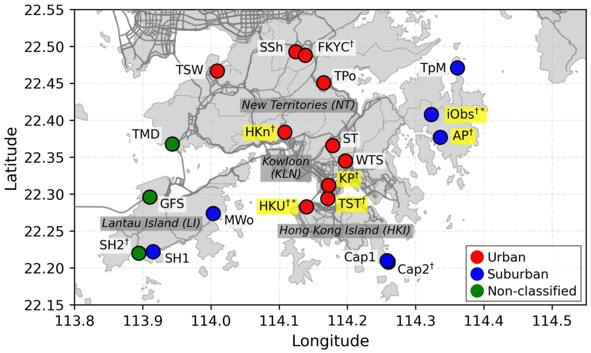
To investigate the long-term trend of light pollution in Hong Kong, NSB has been monitored at 20 different locations in the city since 2010. This allowed us to thoroughly study the night sky conditions across a range of urban and suburban lighting environments and under all natural and artificial conditions. The monitoring stations were strategically selected to provide balanced coverage of different lighting settings, from densely populated urban areas to suburban locations. The details of the monitoring stations, including their locations, are provided in Table 1 and Figure 1.
In this work, we used data collected in two episodes based on project periods: NSN (on or before March 2013) and GaN-MN (on or after December 2014). Some locations (see Table 1 for details), such as HKU, HKn, TST, KP, AP and iObs, have continuous measurements in both projects. These are “decade-long stations” (total 6). Although their data may have been available during the transition between episodes, they were excluded from this study to ensure data quality. Observations at certain locations, including TPo, TSW, WTS, SSh, ST, MWo, TpM, TMD and GFS, were concluded after the first project. Conversely, the second project introduced new locations, such as FKYC, Cap2 and SH2. Together with the six decade-long stations, there are nine “current analysis stations” in total, and the data from these stations are analyzed in detail in this paper.
Each location is roughly classified as urban or suburban according to the land use in the vicinity of the location (published as the map “Land Utilization in Hong Kong” and available here: https://www.pland.gov.hk/pland_en/info_serv/open_data/landu/ (accessed on 25 April 2026)). The urban/suburban classification follows the conventions established in [15,39], in which rural locations are renamed suburban, according to the Bortle dark-sky scale [74]. In special cases where the locations are close to a port facility (TMD) or an airport (GFS), we considered them as non-classified, i.e., neither urban nor suburban. See [15] for additional details. The recent location SH2 is also considered as a non-classified location, as described below.
A special note for Hong Kong geography follows: As a coastal city, the landmass of the Hong Kong Special Administrative Region has three geographical regions, namely (from south to north), Hong Kong Island (HKI), Kowloon (KLN), and the New Territories (NT). The NT also include around 200 outlying islands, of which Lantau Island (LI) is the largest. Immediately to the north of the NT is the city of Shenzhen in Guangdong Province, on the Chinese mainland.
Pun et al. [15] described some of the locations listed in Table 1. We describe below the current analysis stations that were not included. In particular, two stations (SH, Cap) were moved to new installations. Since the new stations are within the same regions as the previous one, we reused their location codes, with the order specified as 1 (old locations) and 2 (new locations).
FKYC
This station is installed on the roof of a high school located near the boundary of a residential town—namely, Fanling (249,535 population, together with the nearby districts Sheung Shui and Kwu Tung, in 2021 [75]), northern NT. The town has livelihood facilities such as shopping malls, markets, parking lots, schools, temples, housing estates, and a train station (∼430 m). A housing construction site with safely lighting, which was active during the study period, was located across the street from the school. Before September 2022, we used the SQM-LU-DL (optically identical to the SQM-LE). Data were stored locally, and the unit was battery-powered, which led to gaps in sampling whenever the battery was depleted.
Cap2
The previous location (Cap1) was located at a marine science research center lying on the shore of Cape D’Aguilar, the southern remote tip of HKI. Since the commencement of the research center’s renovation, we moved the monitoring equipment to the Cape D’Aguilar Radiation Monitoring Station (Cap2), operated by HKO. Within the marine reserve area with the minimum ALAN, the old and new locations are located on the same cape but separated by ∼270 m. The HKO’s station is unmanned, and the only main light source is a lighthouse located ∼100 m away.
SH2
The previous location (SH1) was at a private astronomical observatory. We moved the monitoring equipment ∼2 km west to the Shek Pik Tide Gauge Station (SH2) operated by HKO in Shek Pik, southern LI. The unmanned gauge station is located near a small pier in Tong Wan Bay. The primary light source is the security lighting of the Shek Pik Prison ∼300 m north. Further north of the prison is the dam of the Shek Pik Reservoir. Given its unique setting, we consider SH2 to be a location with a non-classified environment.
The amount of cloud was observed at the urban location HKU (university campus) and the suburban location iObs (astronomical observatory). Their locations are marked in Figure 1.
Recently, we have started monitoring the NSB at two additional northwestern locations in the NT: Tsim Bei Tsui (location code: TBT), and within the Mai Po Nature Reserve (MP). Situated within the Mai Po Inner Deep Bay Ramsar Site, these new locations aim to assess the impacts of ALAN—including those diffused from the city of Shenzhen across the border—on wetland habitats. We will discuss the results obtained from these locations in a separate publication, which is currently in preparation.

2.2. Observing Equipment and Data Quality Control

2.2.1. NSB

To automatically measure and report the zenith NSB from the monitoring network, we utilized SQM-LE photometers that measure and report NSB readings in the astronomical logarithmic unit of magnitude per square arcsecond (mag arcsec−2) every 30 s; each individual measurement takes less than one second. In this convention, a brighter night sky corresponds to a smaller numerical value, and vice versa.
The designation “L” indicates that these sensors incorporate a lens element, which narrows the full width at half-maximum (FWHM) of the angular sensitivity to approximately 20°. The designation “E” denotes the Ethernet connectivity of the instruments, which facilitates automated data transmission over the internet from the monitoring network.
The spectral sensitivity, angular response, photometric accuracy, linearity, temperature stability, and other performance characteristics of these sensors have been extensively studied and documented in the literature [19,20,39,76,77,78,79,80,81,82,83].
The SQM-LE sensor is a monochromatic photometric device, meaning that it provides a response based on the total incoming light intensity, rather than measuring specific wavelengths. As a result, the measured NSB values represent an integrated sum of energy contributions from various outdoor lighting sources of different types, brands, and models, combined with natural emissions from atmospheric gases and molecules, as well as astronomical sources like the Moon and planets.
To maximize the quantity of usable data while ensuring high quality, raw NSB measurements were subjected to a three-level quality control process. First, any data collected during periods of known non-routine human activities were filtered out, such as firework displays, festival light shows, or instances of sensor testing. This initial filtering step helped remove measurements that did not accurately reflect the normal night sky conditions.
The second level of quality control filtering concerned data entries collected under the influence of sunlight. Each monitoring station operated daily from before sunset to after sunrise. However, to ensure that the measurements only reflected the true night sky conditions, data collected outside the astronomical dark period were excluded. Astronomical dark is defined as the period when the Sun’s altitude is 18° or more below the horizon, which in Hong Kong translates to 74 to 86 min after sunset and before sunrise throughout the year. During this astronomical dark period, the sky is completely free from any influence of sunlight.
The third level of quality control concerns moonlight. In addition to sunlight, the sensors also captured moonlight when the Moon was above the horizon and the sky was not completely overcast. To study the influence of moonlight on NSB data, we classified each sunlight-free data point into two categories—moonlight-affected and moonlight-free—as described by [15]. We defined the moonlight-affected period as when the lunar phase was larger than 0.2, and conversely the moonlight-free period as when the lunar phase was smaller than or equal to 0.2—the cutoff value confirmed with sensitive threshold testing. The AP data demonstrated that the 99th and 95th percentiles, as well as the average zenith NSB, are unaffected at lunar phases below 0.2. Statistically significant changes emerge only above this threshold. Given that AP is the darkest site and, thus, the most susceptible to lunar interference in our study, this criterion is conservatively justified across all other monitoring locations for this work. Moreover, it is not necessary to treat lunar altitude as a separate variable, since lunar altitude and lunar phase carry a systematic relation for any given time of night (e.g., the Moon at 0.2 phase is necessarily confined to low altitudes, typically below 30°, and cannot appear high in the sky). Hence, adopting the cutoff for one effectively restricts the other. The lunar phases were calculated using the Alcyone Ephemeris software version 4.3, which was programmed to calculate lunar phase data accurately to the nearest 15 min. Since the comprehensive study of Moon–NSB interactions has already been presented in [15,39], we only utilize moonlight-free observations in this study.
New sensors were calibrated with a claimed accuracy of 0.1 mag arcsec−2, or roughly 10% of the brightness of the sky in terms of emitted flux [83]. The manufacturer conducted multiple rounds of sensor checks. This process involved estimating the light attenuation caused by aging optical components—specifically, the IR-cutting filter, the lens plate in front of the sensor, and the glass window of the housing. Collectively, an attenuation of up to 2.5 mag arcsec−2 was observed. However, due to the lack of detailed information on how attenuation changes over time, we did not correct the readings for aging effects. Despite this, the comparisons conducted within short time frames (whether by months or nights) remained robust. See Section 3.4 for details.
Two types of housing were adopted to protect the sensor, which is not intended for direct outdoor operation, against weathering. During the NSN period, a transparent polycarbonate cover was used. However, from early 2012, a glass window was adopted for the GaN-MN and the current study period. The polycarbonate cover and some of the early glass windows were found to have aged under prolonged exposure to sunlight. We compensated for the change in transparency as described in [39].
Lastly, at TST, we wrapped light shields made of a black rubber sheet around the housings during the GaN-MN project period. The top edge of the shield was about 130 mm above the housing’s viewing window. The shield blocked light incoming from zenith angles of about 30° to 40° onward in all directions, to block stray light from nearby sources while keeping the sensor’s field of view (FOV, approximately 20° in FWHM) unobstructed. Compared to a naked sensor, from control experiments carried out in the laboratory and in the field, the shielding attenuated the incoming light from the sky reaching the sensor by 0.76 mag arcsec−2. We applied an offset with the same amount to the TST data prior to analysis.

2.2.2. Cloud Amount

The amount of cloud was estimated with the IR cloud amount obtained by cloud sensors installed at “cloud analysis stations” HKU (cloud sensor 1 with series number 781) and iObs (cloud sensor 2 with series number 880). The cloud sensor model was Boltwood Cloud Sensor II, manufactured by Boltwood Systems Corporation and distributed by Diffraction Limited (https://diffractionlimited.com/product/boltwood-cloud-sensor-ii/ (accessed on 10 January 2024)). The sensor passively senses the effective IR sky temperature T s in the 8–14 μm range within its ∼80° main FOV. The sensor also measures the ambient ground-level temperature T a with the humidistat at the bottom of the device. The difference between T a and T s —namely, T s a —is an indicator of the amount of clouds [84]. The smaller the temperature difference, the more cloudy the sky is, and vice versa [85]. T s a and the total sky emissivity ϵ can be shown to be related by the following relation [86]:
T s a = T s T a = ( ϵ 1 / 4 1 ) T a ,
where ϵ is the combination of the emissivities of the clear sky and the cloud in all layers.
Raw data with a data collection frequency of ∼2 s (which cannot be changed by users) were recorded around the clock. The ±1 min moving median of raw T s a was then extracted to represent T s a every minute. The choice of the ±1 min median smoothing was a compromise between describing the rapid changes in cloud condition and reducing the statistical fluctuations in the received data. Statistical errors during this moving median extraction were defined as one standard deviation (1 σ ) of the spread of the raw values T s a involved in the calculations. The instrumental error on the cloud sensor measurements was assumed to be the last precision digit, or 0.1 K.
Note that this method of cloud measurement does not distinguish clouds of different cloud base heights and cloud types, or high cirrus made of ice crystals. Also, as a non-imaging sensor, the spatial distribution of cloud and partial cloud amount (amount of sky covered by each type or layer of clouds) cannot be measured. Nevertheless, a cross-comparison of HKO’s cloud visual observations and T s a cloud amount indicated consistency ([39], Section 3.4.2.1), highlighting the usefulness of the current method in reliably assessing cloud conditions and supporting further meteorological analysis.
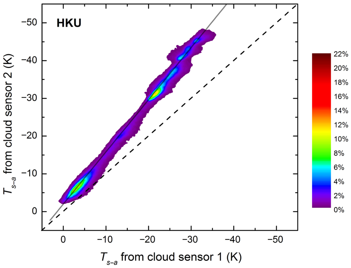
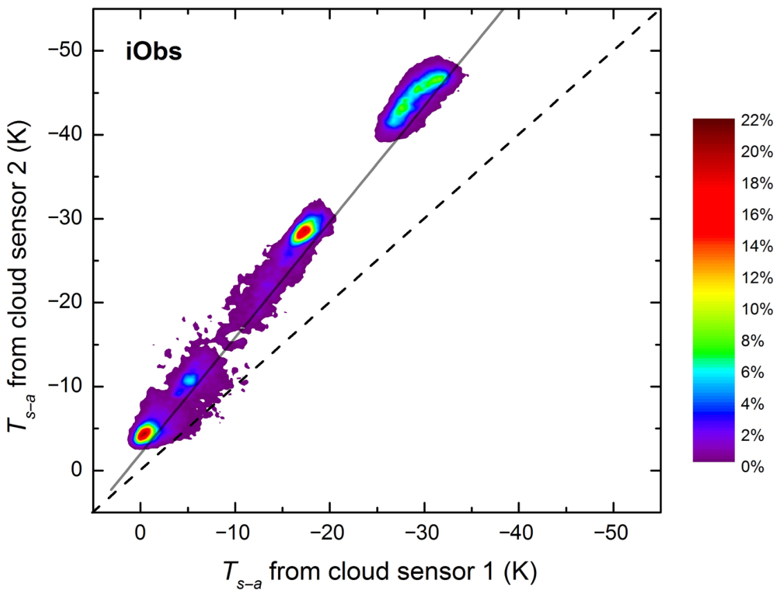
Although the type of cloud sensor at HKU and iObs is the same, they are not calibrated by the manufacturer. The exact value of T s depends on the cloud amount, local conditions, and differences between devices. To define the differences between devices, cross-check experiments were conducted in HKU and iObs separately. The details and results of the experiments are included in Appendix A. The T s a values measured from cloud sensor 2 were transformed to those of sensor 1 with Equation (A1) to correct the discrepancies in the measuring equipment. The effect of nightly temporal variations in NSB due to artificial light was also removed prior to analysis. See Appendix B for details.
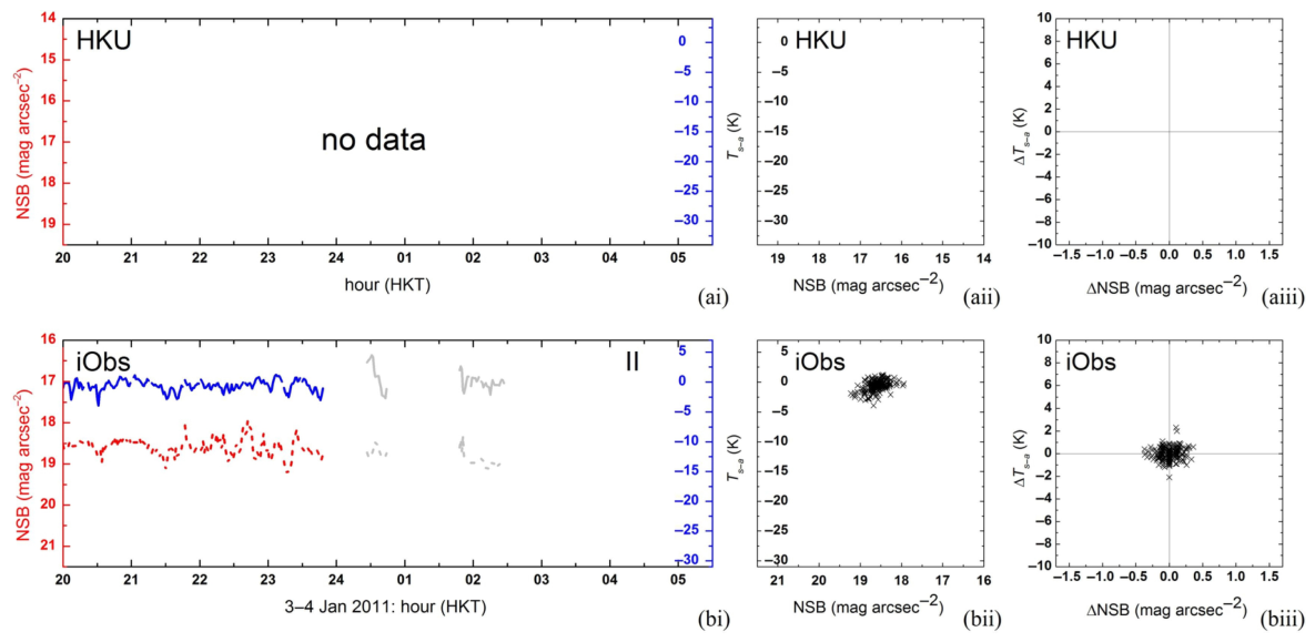
The Boltwood cloud sensor, designed to alert the observer in case of any sign of rain or moisture during observation, can detect rain droplets. By checking the sensor’s data entries, the NSB and cloud data entries taken in rain and after rain for the rest of the night were excluded for the cloud–NSB analysis, but the raining sections of the time series are shown and indicated by gray curves in Section 3.6. It was assumed that the covering optics of the SQM-LE was dried before the start of the next run.
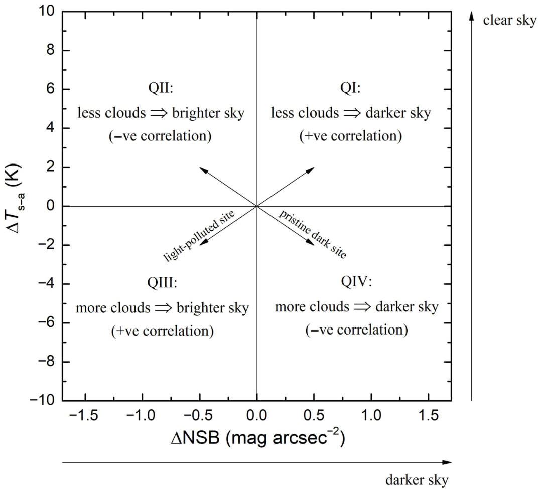
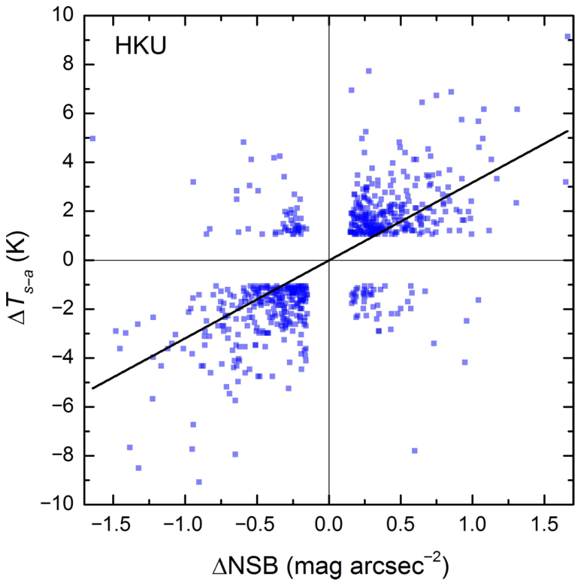
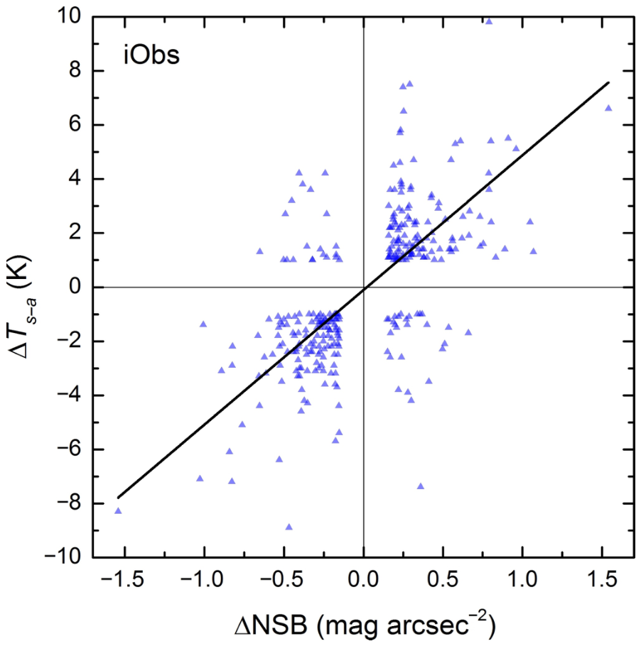
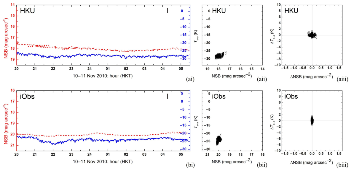
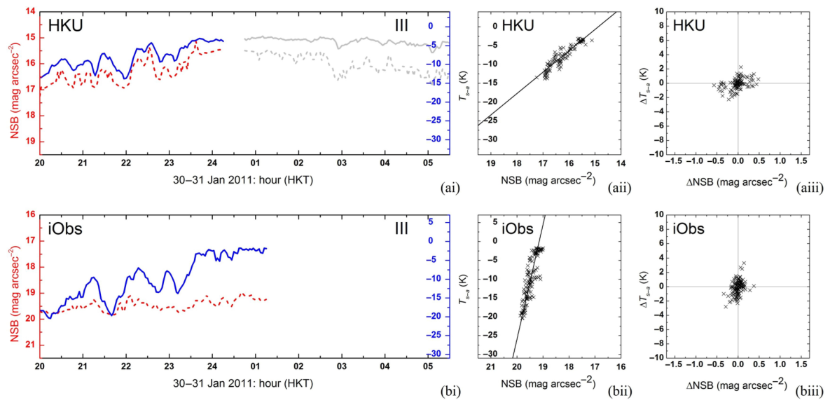
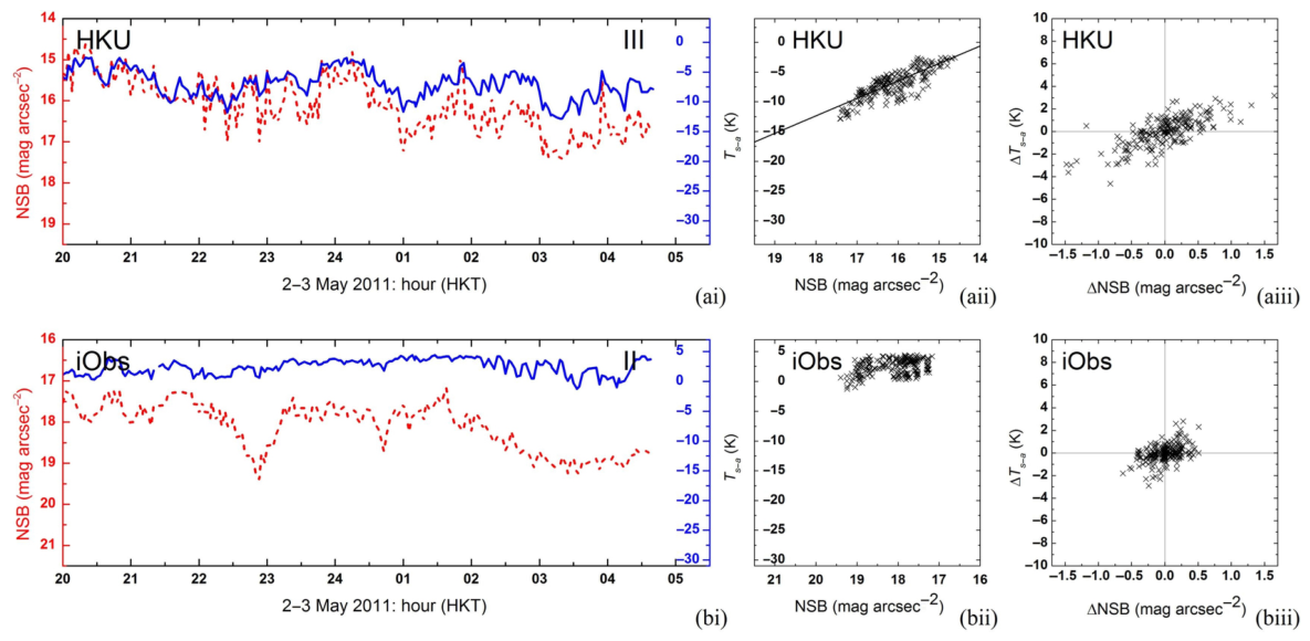
Building on previous work, we analyze and compare T s a with NSB data using several approaches in Section 3.6. In Section 3.6.3, Section 3.6.6 and Section 3.6.7, we examine their correlation by defining Δ T s a = [ T s a ( n ) T s a ( n 1 ) ] and Δ NSB = NSB ( n ) NSB ( n 1 ) , where n is a running data index. The minus sign before the first term in Δ T s a ensures that Δ T s a is positive (negative) for decreasing (increasing) cloud amounts. Positive (negative) Δ NSB indicates a darker (brighter) trend. The phase space plot of Δ T s a versus Δ NSB , as shown in Figure 2, serves as a direct measure of this correlation, i.e., how the temperature difference varies as NSB varies, at light-polluted and pristine dark sites.

3. Results

3.1. Data Statistics

3.1.1. NSB Data

From 2010 to 2023, six monitoring stations—namely, HKU, HKn, TST, KP, AP and iObs—established a decade-long dataset throughout two project periods. Three stations—namely, FKYC, SH2, and Cap2—are new locations that are not discussed in [15]. Here, we provide a statistical data summary on the dataset collected from those nine current analysis stations, and we analyze their NSB geographical and temporal variations in the following subsections. For old locations with datasets collected from 2010 to 2013 (i.e., TPo, TSW, WTS, SSH, ST, SH1, Cap1, MWo, TpM, TMD, and GFS), we will not repeat their statistics, which have already been presented in [15].
During the study period from 1 July 2019 to 30 June 2023, more than 23,550,000 individual raw entries were collected from the nine monitoring stations in Hong Kong, with an overall success percentage (the data collection success percentage for a given night at each station was defined as the number of entries received divided by the number of entries expected between sunset and sunrise.) of 85.4%. After quality control processing (Section 2.2.1), 11,135,616 (47%) data points were sunlight-free, of which 3,252,201 (29%) data points were also moonlight-free. Table 2 tabulates the breakdown of sample size from each monitoring location. We sorted the table according to the average brightness of the sky, from brightest to darkest (Table 3). Note that the statistics include observations made under different cloud conditions.
Established in August 2021, FKYC has substantially fewer data than the other sites. The small sample size resulted from its initial data collection setup: a battery-powered SQM-LU-DL (optically identical to the SQM-LE) that stored data locally, causing gaps whenever the battery depleted. Data coverage improved after the site switched to the mains-powered SQM-LE with fixed-line internet.
In the following subsections, we will present a complete and recent picture of the city’s light pollution, with a series of analysis taking all data taken from individual current analysis stations as a whole first (Section 3.2), and then examining the datasets at a variety of temporal scales, spanning from 5 min (Section 3.3), through a night (Section 3.4), to a month (Section 3.5). Additionally, to reveal the decade-long change in the conditions of light pollution in the entire city as a whole, we will include the data collected for the NSN project before March 2013, for the Δ NSB late early analysis in Section 3.4.

3.1.2. Cloud Amount Data

During the cloud data collection period between November 2010 and May 2011, the sampling frequency of the IR cloud data in T s a was ∼2 s. Every NSB observation (at a rate ranging from 1 to 5 min each) was matched to the closest cloud amount observation. For example, the NSB observed at 00:00:10 was matched to the cloud amount of 00:00:00, which is the median value of raw data taken within 2 s between 23:59:00 and 00:00:59.
Table A1 and Table A2 in Appendix E summarize the observational conditions of the observation runs selected for analysis. There are 39 and 38 runs sampling 338.0 and 302.5 h for HKU and iObs, respectively, covering 41 individual nights during the cloud sensors’ operational period. Two nights at HKU and three nights at iObs did not have any data due to hardware and/or software problems. Hereafter, #ID-stations listed in Table A1 and Table A2 will be used to refer to specific runs.
It should be noted that all of the NSB data utilized in the cloud-NSB study are also free from sunlight (observed between 20:00 and 05:30) and moonlight (observed when the lunar phase < 0.2).

3.2. Geographic Variations in NSB

Table 3 presents the average sunlight- and moonlight-free NSB and its spread in 1 σ at each of the current analysis stations. The table is sorted in descending order from the brightest to the darkest sky locations. The last column in the table lists the number of times the NSB at each location exceeded the dark sky standard established by the IAU. This standard, set at 21.6 mag arcsec−2, defines the natural zenith V-band NSB level for a good astronomical site without light pollution from ALAN, as defined in [40] (reproduced as Appendix 4.1 in [87]). Note that this standard does not account for the solar cycle. Previous studies have shown that NSB varies over the solar cycle and reported a natural zenith limit of ∼22 mag arcsec−2 during the solar minimum ([88,89,90,91,92,93], for example).
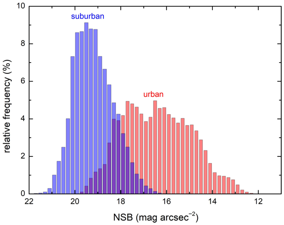
In general, the night skies in Hong Kong were found to be very bright during the study period. On average, in all current analysis stations, the night sky was 43× brighter than the dark sky standard established by the IAU. When the analysis was separated into urban and suburban locations, the differences became even more stark. Urban locations were on average 119× brighter than the dark sky standard, while suburban locations were 9× brighter. This huge disparity, with the urban skies about 13× brighter than the suburban skies, signifies the highly heterogeneous distribution of ALAN and the resulting light pollution conditions in different parts of the city.
At the brightest location monitored, King’s Park (KP) in KLN, the night sky was found to be around 250× brighter than the IAU dark sky standard. This is not surprising, given that KP is situated in the heart of the Kowloon Peninsula and receives significant artificial light emissions from the densely populated surrounding districts, including Yau Tsim Mong, Kowloon City, and Wong Tai Sin. The extremely bright conditions at this urban core location underscore the severe impact of light pollution in Hong Kong’s most densely developed areas.
In contrast to the extremely bright conditions at the urban King’s Park location, the darkest site monitored was Astropark (AP) in Sai Kung Country Park, eastern NT. In AP, the night sky was found to be only 6× brighter than the dark sky standard. This relatively dark environment was attributed to the controlled lighting conditions within the park itself, as well as the remoteness of AP from the nearest town of Sai Kung, located ∼6.5 km away. However, even at this level of light pollution, complete dark adaptation of the human eye could only be marginally achieved, as described in a previous study [39]. Additionally, the Milky Way was still barely visible most of the time at the AP site, illustrating that while it represented the darkest monitored location, significant light pollution persisted even in this relatively remote area.
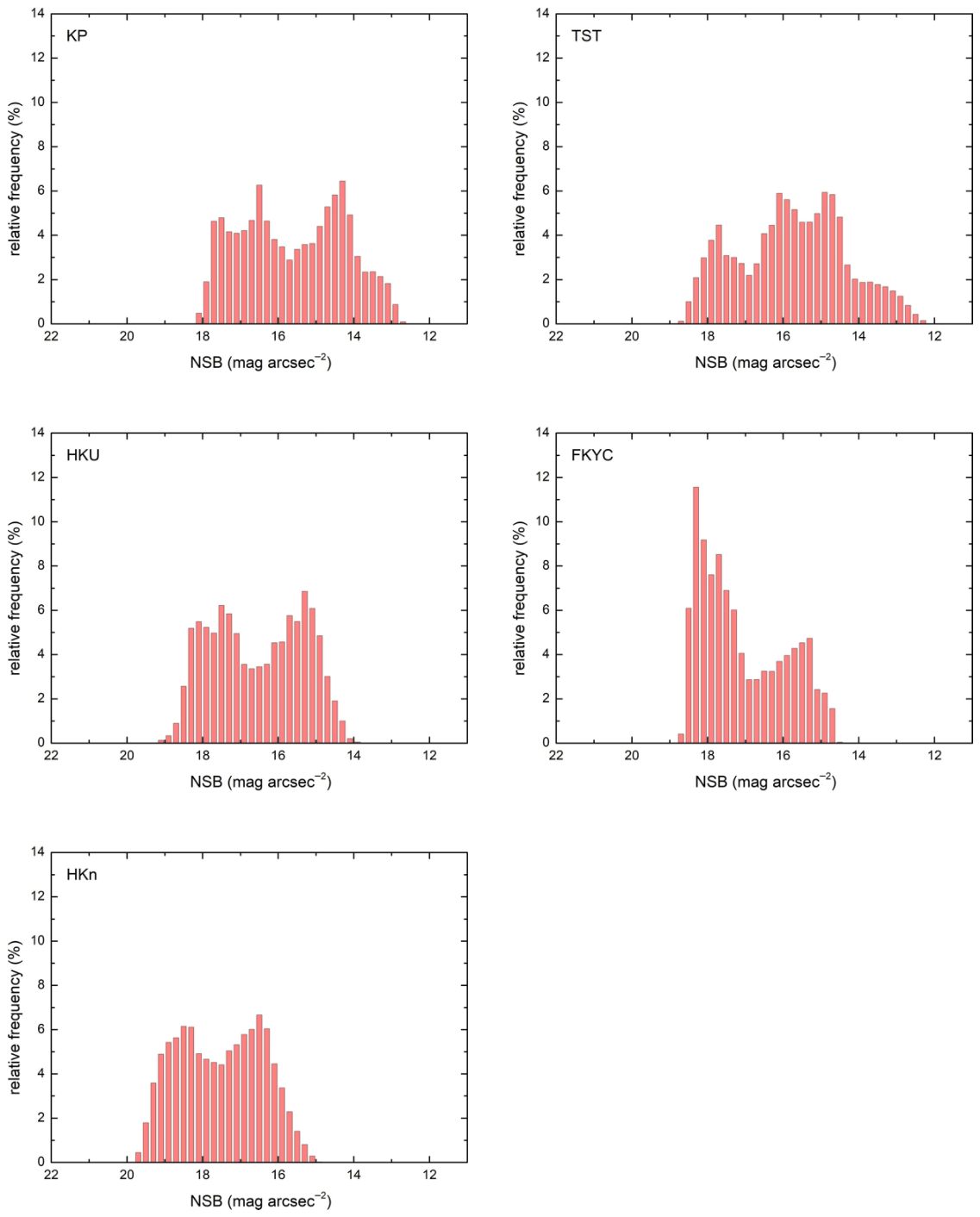
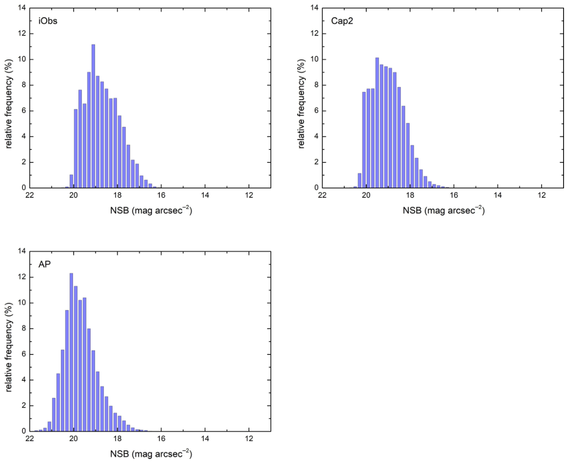
The differences in light pollution between locations can be further examined using the histograms of the NSB values in Figure 3 and Figure 4. Unlike the statistics presented in Table 3, which focus solely on central tendencies, the histograms reveal the actual data distributions. In particular, the histograms do not exhibit characteristics of normal distribution. The range of NSB values observed for each setting type is substantial, ranging from 4.4 to 7.4 mag arcsec−2 in brightness difference or more than 55× in observed luminosity, reflecting the significant inhomogeneities of the conditions under which these data were collected. Urban measurements show greater variability than suburban measurements. Urban measurements are also characterized by two main peaks, highlighting the influence of clouds on observations (see Section 3.6 for details). In contrast, suburban locations display single peaks in general, with the data distribution skewed toward the brighter end. In particular, the AP histogram shows a weak double-peak pattern with very similar peak values, attributed to cloud influence. Our observations align with those of previous studies conducted at various locations ([18,42,49,53,94,95], for example). The combined histograms of the NSB recorded in each land setting are presented in Figure 5. It is evident from the Figure that skyglow from urban lighting sources significantly brightened the night sky, as indicated by the distinct distributions of the urban and suburban data collected under similar atmospheric conditions.
In general, this set of histograms aligns with those presented in [15] (Figures 8 and 10) covering the observation period from May 2010 to March 2013). However, upon closer comparison, the data distributions for KP, TST, HKU, and HKn have shifted slightly toward the darker end after a decade. This shift is particularly pronounced for HKn, where skies darker than 19 mag arcsec−2 were observed after 2019. The step size analysis in Section 3.4 will provide additional insights into these decadal changes.
Due to its unique lighting environment (Section 2.1), SH2 data are excluded from the histograms in Figure 3, Figure 4 and Figure 5.

3.3. Nightly Temporal Variations in NSB

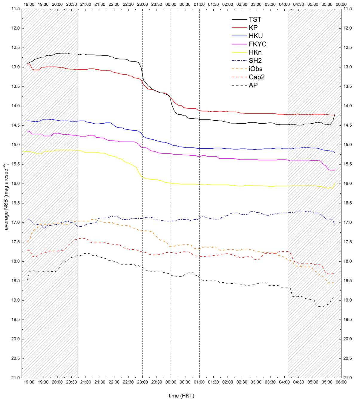
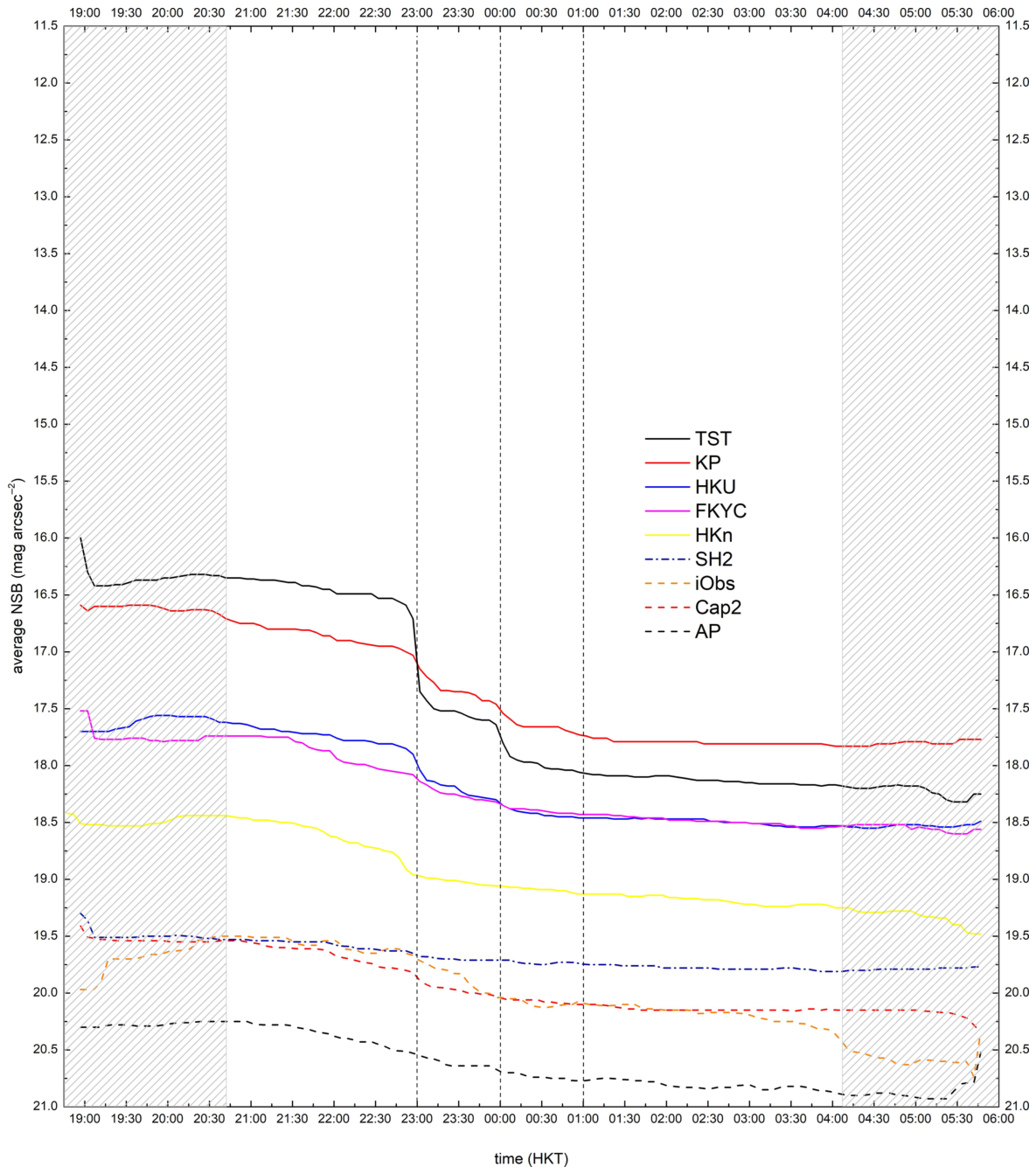
To analyze short-term NSB trends at each location, we calculated the 5th and 95th percentiles of NSB values within rolling 5 min windows. This percentile approach allows us to represent nightly trends while minimizing the influence of extreme readings caused by transient events, such as sensor obstructions (e.g., insects), accidental direct light exposure, or lightning. The 95th percentile (with the 5th percentile as its lower-bound mirror) is also used in high-energy astrophysics to identify unusually bright flaring events in observed flux density [96,97,98]. In addition, by analyzing our large NSB database, this approach also accommodates random cloud fluctuations, hereby revealing the patterns of ALAN usage across the city, in which lighting dimming follows a consistent pattern, despite the absence of cloud observations. The resulting 5th- and 95th-percentile light curves represent the brightest (typically during overcast conditions) and darkest (usually during clear skies) profiles for each location, respectively, accounting for the cloud amplification effect (Section 3.6). In essence, the darkest 95th-percentile clear sky profile serves as a robust indicator of light pollution, reflecting only the true impacts of ALAN on the night sky.
The 5th-percentile light curve, presented in Figure 6, depicts the variations in NSB at each location every night. All light curves, except for SH2, exhibit a clear darkening trend throughout the evening, signifying the gradual reduction in human activities. The darkening is apparently larger for urban locations like KP and TST, implying larger reductions. Significant drops in NSB are obvious at particular times, including 23:00, 00:00, and 01:00, indicating that some external lighting fixtures are probably controlled by timer switches. Regarding the darkening levels, the light curves of urban locations are significantly brighter than those of suburban locations. This observation aligns with the average NSB presented in Table 3 and the histograms presented in Figure 3, Figure 4 and Figure 5.
The 95th-percentile light curve, presented in Figure 7, resembled most of the main features of the 5th version (Figure 6). The shifting of each light curve indicates the cloud amplification effects, which have been statistically removed from the 95th-percentile calculations. In particular, the level differences among light curves were significantly reduced after 01:00, with the NSB grounding at the lowest possible levels, aligning with expectations based on human activity patterns. In other words, that section of the light curve indicates the intrinsic ALAN impacts, without the influence of clouds and moonlight.
The KP’s and TST’s light curves are interesting. Before 23:00, TST is consistently brighter than KP. The situation gradually reverses between 23:00 and 00:00, and finally KP becomes brighter than TST after 01:00. In So [39] (Figures 3.25 and 3.26), TST was consistently brighter than KP throughout the evening in 2010–2013, as shown by the darkest profiles. A decade later, new observations indicated an overall change in the lighting environment. As discussed in Section 3.4, this reversal may be due to greater darkening at TST after midnight and/or reduced darkening at KP after midnight in recent years. Regardless, the interplay between these two light curves can be visualized from neither average values (Table 3) nor histograms (Figure 3), which makes nightly light curves particularly useful in revealing short-term variations in NSB.
Unlike the dimming trends observed from other locations, SH2’s 5th-percentile light curve shows a slight and gradual increase in sky brightness throughout the evening (∼0.1–0.2 mag arcsec−2 per hour), while its 95th-percentile curve remains steady at approximately ∼19.7 ± 0.1 mag arcsec−2. As mentioned in Section 2.1, SH2 is located near the Shek Pik Prison. The unique characteristics of SH2’s light curves can reasonably be attributed to this location, where the prison’s security lighting—which appears not to be switched off or dimmed—likely plays a significant role.

3.4. Variations in NSB Before and After Midnight

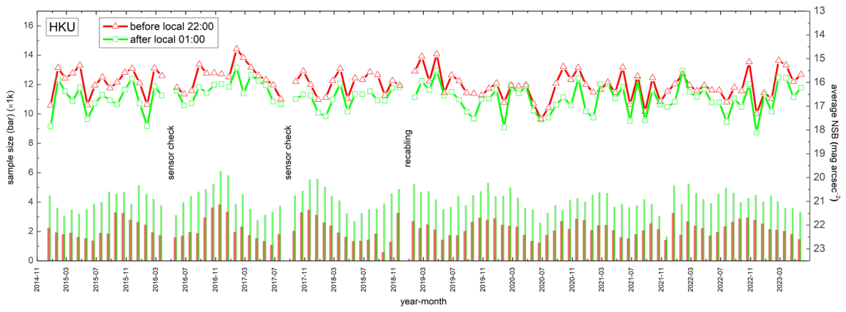
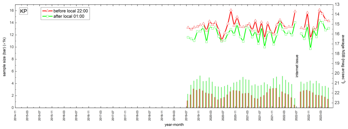
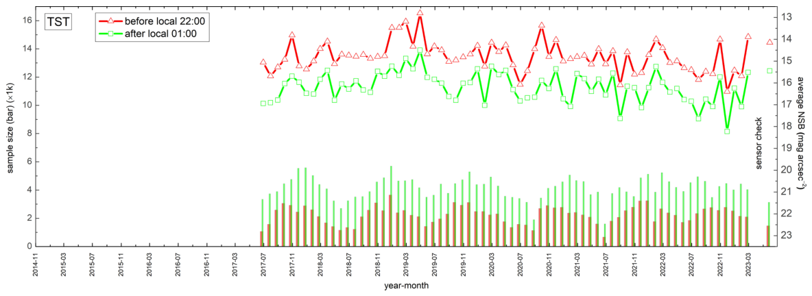
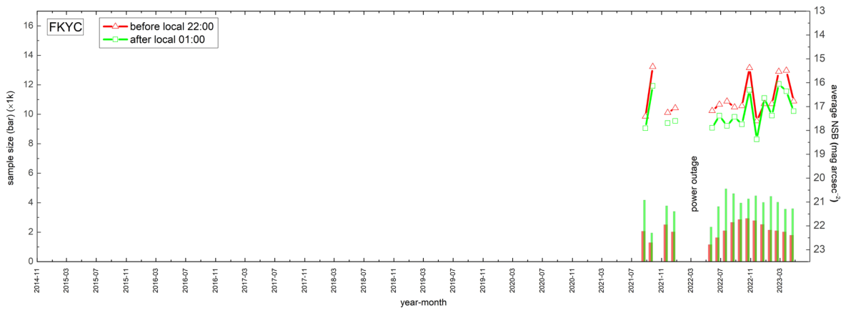
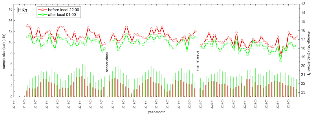
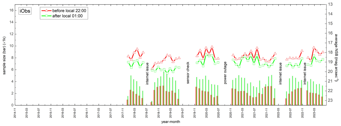
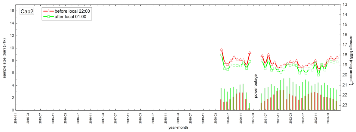
To further quantify the nightly variations in NSB, we calculated the average values for the early evening (before 22:00) and late night (after 01:00) separately for each location and month. This approach takes advantage of the natural decline in human activities after midnight, which can help reveal patterns in the NSB data. The study period was expanded by including NSB data collected between December 2014 and June 2019. This allowed for a long-term analysis of light pollution conditions at several key locations near the six decade-long stations in Hong Kong. The expanded dataset serves as a valuable follow-up to previous studies on light pollution in Hong Kong [15,16,38,39,41]. By leveraging this broader temporal coverage, the analysis can provide deeper insights into the long-term trends and changes in the region’s night sky quality.
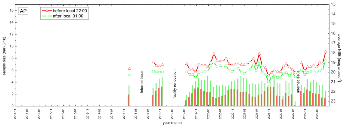
The time series of the nightly variations in NSB is presented in Figure 8 and Figure 9 for HKU and AP, respectively, as examples. The plots of other current analysis stations are presented in Appendix C. All figures are plotted with the same x-axis scale to facilitate easier comparison between the different locations.
Due to its unique lighting environment (Section 2.1), SH2 data are excluded from this presentation.
The presented time series of NSB data reveal several important general trends:
  • Early-Evening vs. Late-Night NSB: The early-evening skies (before 22:00) were generally and stably brighter than the late-night skies (after 01:00), indicating that more external lighting was used and, hence, more light pollution occurred before midnight.
  • Urban vs. Suburban NSB Differences: Urban locations exhibited a larger difference between early-evening and late-night NSB within the same month, compared to suburban locations. This suggests that the reduction in light pollution overnight was more pronounced in urban areas than in suburban areas (more discussions with Δ NSB late early below).
  • Seasonal Variations in Sample Size: The monthly sample sizes were generally larger in winter (longer nighttime duration) than in summer (shorter nighttime duration), exhibiting a periodic variation due to the seasonal changes in the duration of astronomical night throughout the year.
  • Sample Size Differences: Late-night samples (∼3–4 h of data) were larger than early-night samples (∼2–3 h of data) for the same month, as the data affected by sunlight had been excluded from the analysis.
The trends observed in the presented time-series data are consistent with previous discussion (Figure 6 and Figure 7) and previous studies on NSB and light pollution in the region [15,16,38,39,41], corroborating the understanding of the spatial and temporal patterns of ALAN.
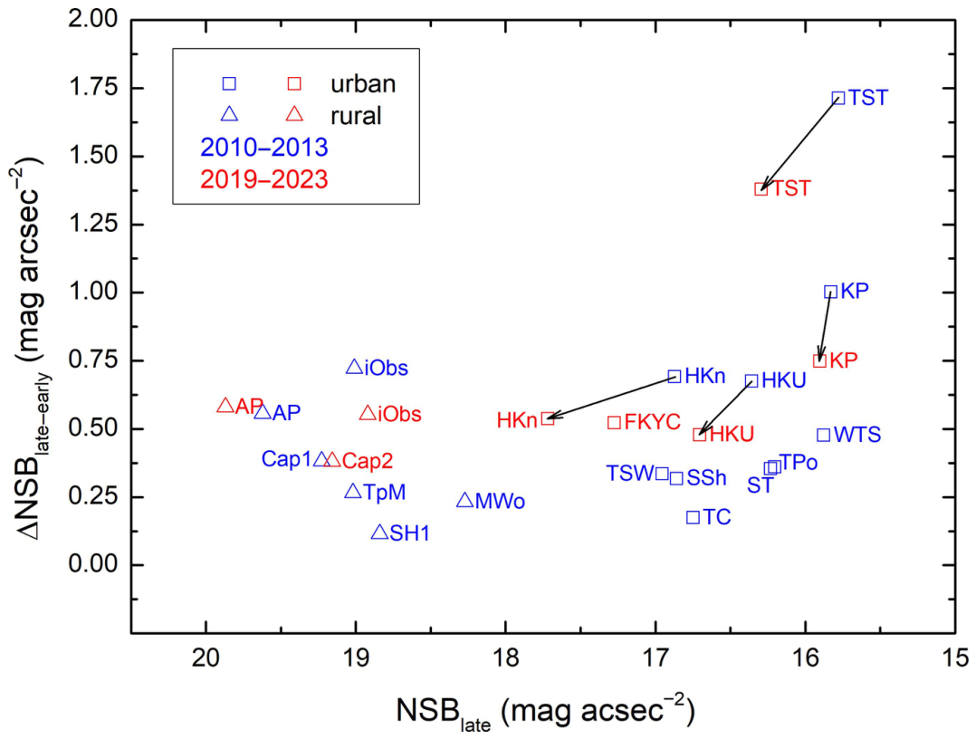
To further quantify the nightly changes in NSB, we calculated the average NSB recorded between 20:20 and 22:45 (early evening) and between 01:15 and 04:45 (late night) for each urban and suburban location and night, when data was available. For individual nights with both early-evening and late-night data, we calculated the difference between the two averages (late − early). We then represented the average of this difference as Δ NSB late early for each location. The metric Δ NSB late early is considered to be a more robust indicator because it is not influenced by changes in instrument configuration or potential sensor degradation, as described in Section 2.2.1. Separated into two datasets that span more than a decade, the scatter plot of Δ NSB late early versus the average late-night NSB ( NSB late ) is shown in Figure 10.
Figure 10 is informative, illustrating not only the light pollution at each location but also its evolution over the past decade. First, Δ NSB late early (step size) indicates how many external lights would be turned off after midnight. In other words, a large Δ NSB late early signifies more non-essential lighting, while a smaller value indicates less. Second, the average NSB late reflects the amount of essential lighting that must remain on for purposes such as road safety, security, and emergency services.
Except for TST in 2010–2013 and 2019–2023, and KP in 2010–2013, the sizes of the steps are all smaller than 0.75. All locations have positive step sizes, meaning that their late nights are generally darker than their early evenings. In particular, the two brightest locations have the biggest steps: TST (1.71 in 2010–2013; 1.38 in 2019–2023) and KP (1.00 in 2010–2013; 0.75 in 2019–2023). They are located in the center of the commercial area of the city, packed with many hotels, shopping centers, and tourist attractions. A large amount of lighting is expected to be in operation before midnight nearby, with much equipment spilling light upward for commercial and decorative purposes.
Most importantly, the shift in the data points of decade-long stations in the scatter plot demonstrates how the conditions of light pollution have varied for non-essential versus essential lighting over a long period of time. In particular, urban data points (i.e., TST, KP, HKU, and HKn) consistently shifted significantly to the lower left, indicating smaller Δ NSB late early and darker after-midnight sky brightness over the past decade. In contrast, suburban data points (i.e., iObs, Cap1, Cap2, and AP) showed only slight shifts and did not exhibit a consistent trend. The darkening in urban locations is consistent with the observations noted in Section 3.2 when comparing histograms across a decade.
In urban locations, the shift to the lower left could be related to the successful implementation of external lighting guidelines, particularly the Charter on External Lighting (Charter) [99]. This initiative encourages owners and persons in charge of external lighting to switch off decorative, promotional, or advertising lighting during preset times before midnight (project website: https://www.charteronexternallighting.gov.hk (accessed on 25 April 2026)). Since the launch of the Charter in early 2016, participation has expanded substantially, growing from approximately 1000 signatories to 5200 by 2024 [100]. Notably, the observed darkening of urban skies within the second epoch of NSB data (2019–2023) aligns temporally with both the Charter’s establishment and the subsequent steady increase in adherence. While external factors, including meteorological and air-quality shifts, economic drivers, and solar cycles, may contribute to overall NSB variations, our findings suggest that the Charter’s implementation is indeed a possible contributor to the recorded reduction in light pollution. Consequently, our data support the potential efficacy of voluntary guidelines in managing urban light pollution.
Upon closer examination, TST and KP exhibited similar NSB late values from 2010 to 2013. After a decade, TST experienced a more significant decline in NSB (indicated by a larger shift in Δ NSB late early ) compared to KP, resulting in approximately 0.4 mag arcsec−2 brighter NSB late at KP during the 2019–2023 period.
Additionally, the KP and HKn data pairs from the two study periods reflect two distinct types of decadal changes. Over the course of a decade, KP exhibited minimal variation in NSB late (+0.07 mag arcsec−2), accompanied by a significant reduction in Δ NSB late early (−0.25 mag arcsec−2). In contrast, HKn experienced a notable darkening in NSB late (+0.85 mag arcsec−2), with only a slight change in Δ NSB late early (−0.15 mag arcsec−2).
The differences in decadal changes between the two locations highlight how the use of ALAN varied in these urban settings. Our observations suggest that, while overall ALAN usage near KP remained largely stable over the past decade (as evidenced by the minimal change in NSB late ), more ALAN was turned off after midnight (as indicated by the significant reduction in Δ NSB late early ). In contrast, there was an overall decrease in ALAN usage and/or a reduced upward light spill near HKn (evidenced by the considerable darkening of the sky), but there was only a slight change in lighting practices during the same period (as indicated by the minimal variation in Δ NSB late early ).
To evaluate the robustness of our findings, a sensitivity analysis was performed by subsampling data from the last half of each observation epoch (October 2011–March 2013 and January 2021–June 2023). The results indicate that the primary conclusions remain consistent regardless of the specific time window selected. Although marginal shifts in individual data points were observed, likely representing the extent of their systematic uncertainties, the overall direction and magnitude of the Δ NSB late early shifts for all decade-long stations remained consistent. This confirms the statistical robustness of our analysis and supports that our main conclusions remain unchanged regardless of the specific time window selected.
On the other hand, the observed decadal decline in NSB may be due to several factors, including reduced use of non-essential lighting near the observation site (likely driven by economic reasons), improved lighting practices (such as better shielding), and light-emitting diode (LED) retrofitting (since the sensor is less sensitive to the blue emission of LEDs). Further discussion is provided in Section 4. In addition, the change in direction between 2010–2013 and 2019–2023 may be attributed to the transition from Solar Cycle 24 (2008–2019) into the rise of Cycle 25 (since December 2019) [101], since previous studies have shown that NSB at dark sites varies with the solar cycle ([88,89,90,91,92,93], for example).

3.5. Monthly Temporal Variations in NSB

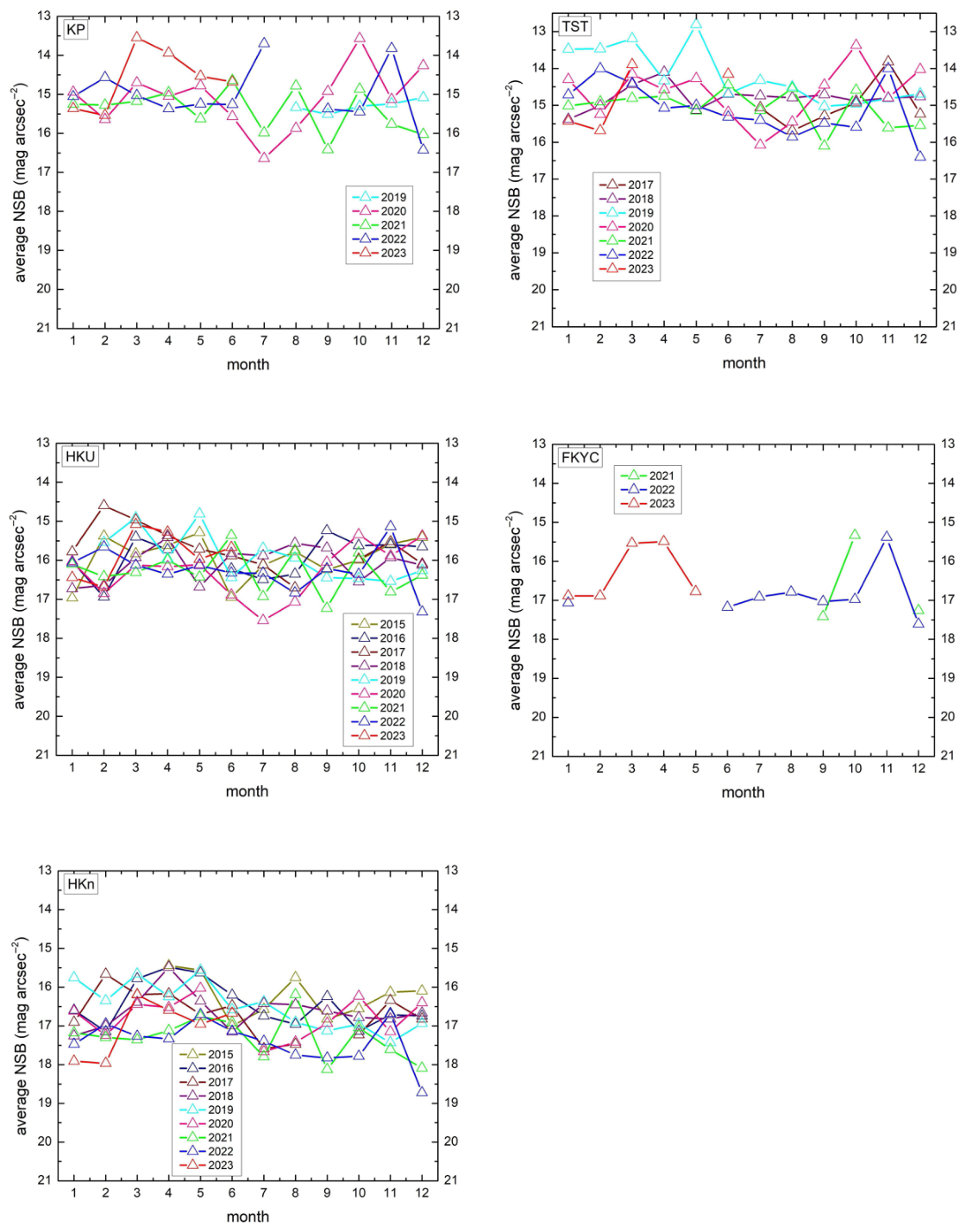
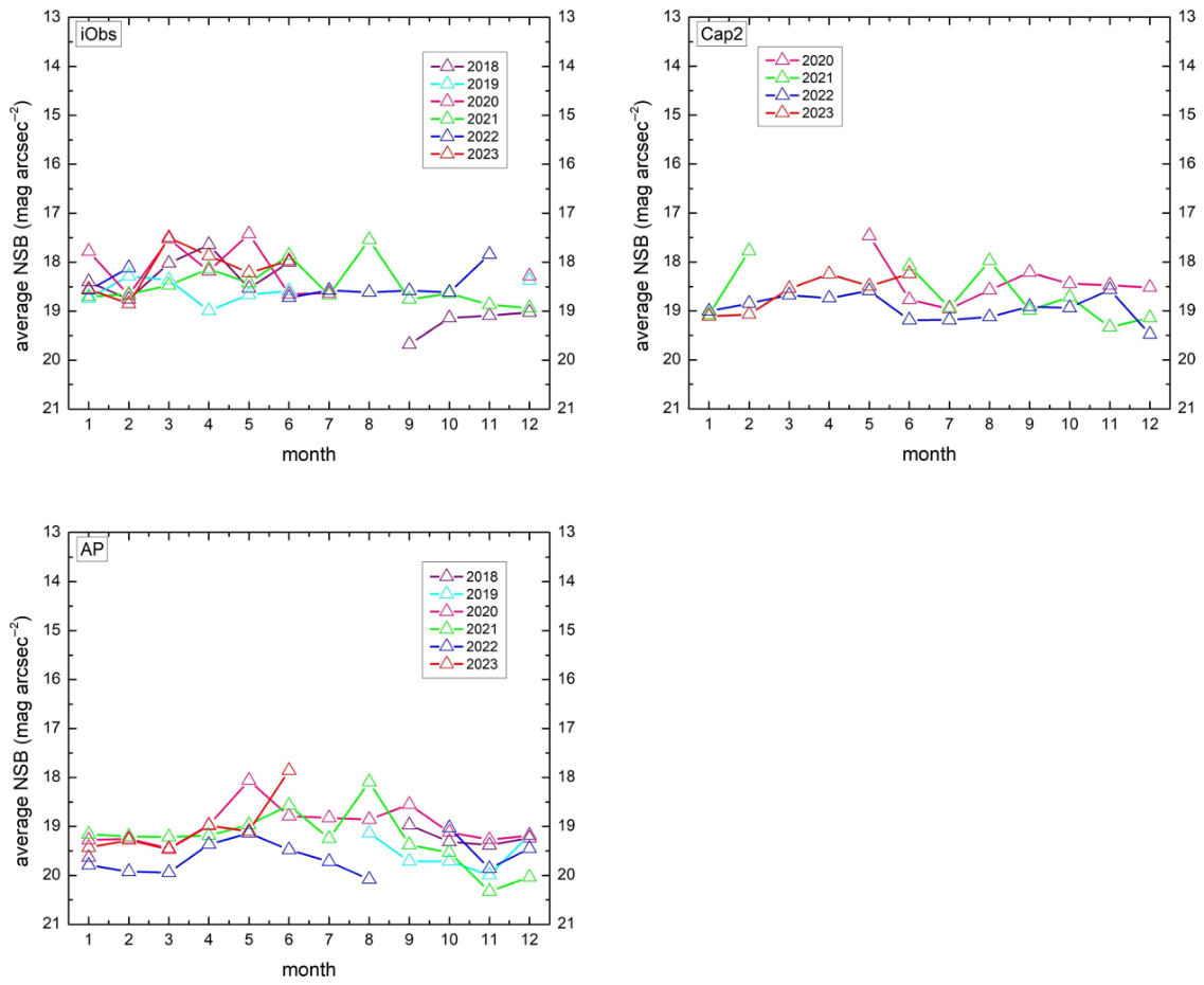
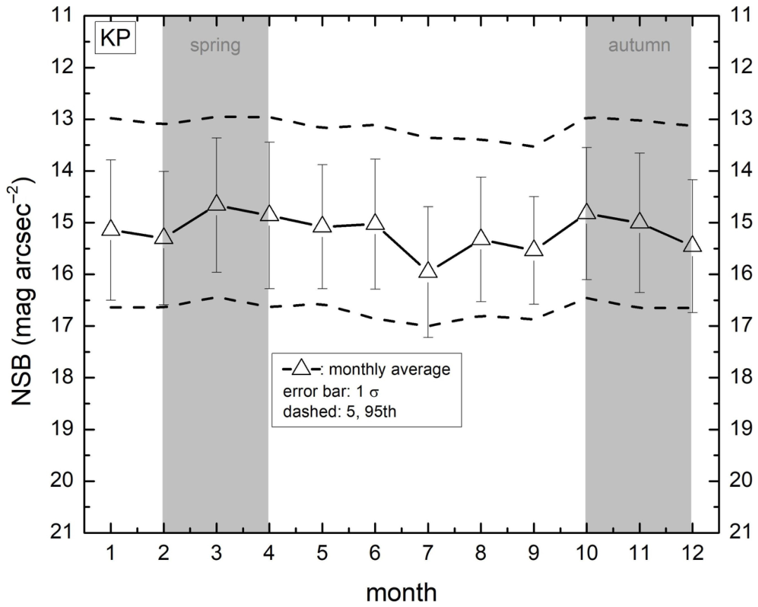
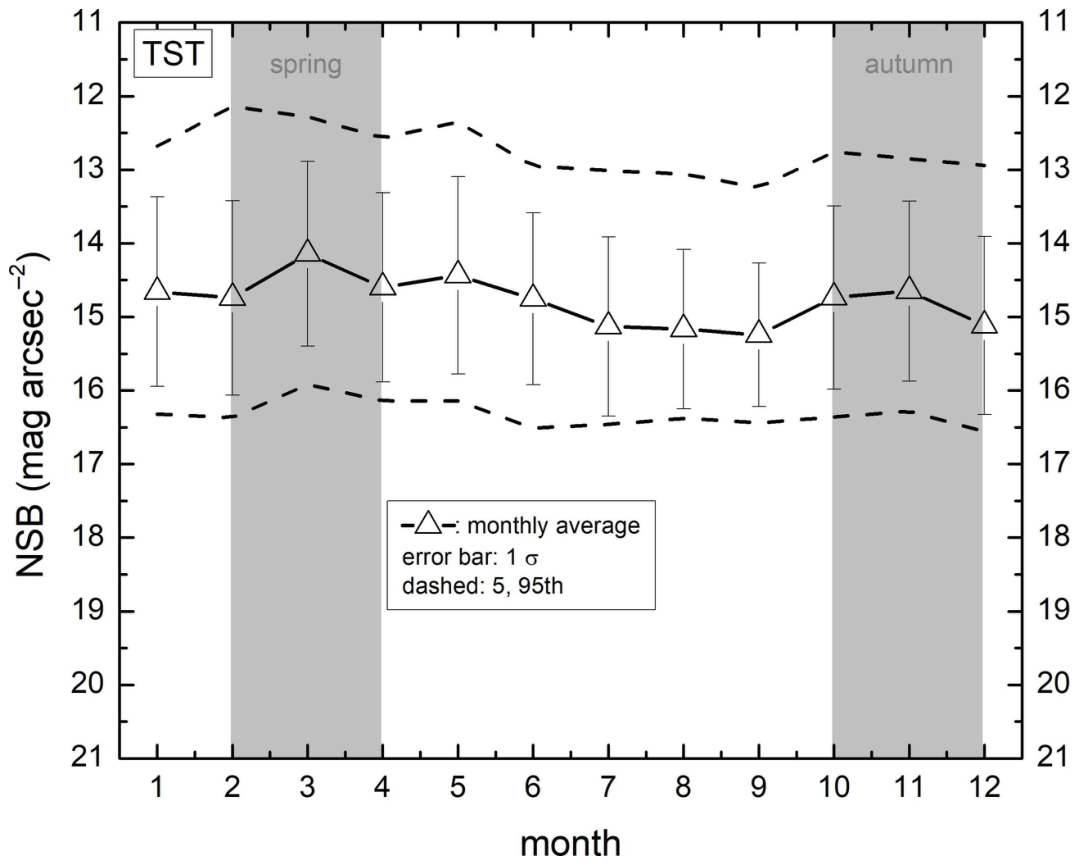
To study the monthly variations in NSB from the expanded database, we calculated the average early-evening (before 22:00) NSB values collected at each location for the same month. We focused on the early-evening data because it is more representative of the light pollution conditions at specific locations before the decline in human activity near midnight. We plotted the average NSB values against individual months and stacked the values from different years to reveal any seasonal trends in Figure 11 and Figure 12. This approach allowed us to gain insight into the seasonal patterns and monthly variations in light pollution at the monitored locations.
Due to its unique lighting environment (Section 2.1), SH2 data are excluded from this presentation.
Some of the time series in Figure 11 and Figure 12 contain many data points, especially for locations with many years of data. To better show the annual trends, we provide a simplified version of the figure for KP, TST, HKU, and HKn separately in Appendix D.
Based on the monthly time-series data, we identified several general trends:
  • Some locations exhibited a weak periodic trend, where spring (February–April) and autumn (October–December) were brighter, while summer (June–August) was darker in general. Based on the cloud–NSB relationship and the known seasonal cloud amount variation in Hong Kong (more clouds in spring [102]), this periodic trend can be partially explained by the seasonal changes in cloud amount.
  • The same months across different years exhibited varying NSB values at the same location. This is not surprising, as the measurements included scattered light from clouds, and we did not separate the NSB data collected under different cloud amounts (more details in Section 3.6). Therefore, the varying cloud amounts among the same months in different years contributed, at least partially, to the observed differences in NSB.
  • At each location, the data points were distributed within a band of ∼3 mag arcsec−2. Assuming that the external lighting conditions did not vary rapidly month-to-month, and based on the known cloud–NSB relationship, the upper bound of the band defines the overcast NSB level, while the lower bound defines the clear-sky NSB level (more details in Section 3.3).
  • Urban stations (TST, HKU, and HKn) exhibited marginal NSB decreases during 2021–2022, a time frame coinciding with the COVID-19 pandemic. As studies at the global [36,103], national [104], and municipal scales [105,106,107] have reported pandemic-related dimming in commercial ALAN, the observed NSB drops in Hong Kong may be partially attributable to reduced external lighting usage. This aligns with findings by So et al. [25], who noted a reduction in relative darkening during Earth Hour 2021, likely reflecting broader changes in nocturnal lighting activity under lockdown conditions. Post-pandemic data revealed a divergent trend across monitoring sites: while most locations reverted to pre-COVID NSB levels, the HKn station in Tsuen Wan maintained a downward trajectory. This divergence highlights the complex interplay between anthropogenic drivers, such as shifting economic activity and natural variables that influence long-term NSB fluctuations. Consequently, additional research is required to isolate the sustained impact of the pandemic from the transient anomalies introduced by other external factors.

3.6. Impacts of Cloud Coverage on the Observed NSB

Except for the 5th- and 95th-percentile light curves in Section 3.3, the previous analyses included NSB observations under all cloud conditions. In the following subsections, we separate NSB observations conducted at cloud analysis stations by cloud amount and use simultaneous NSB and T s a cloud amount measurements to quantify how the cloud amount influences the observed NSB.

3.6.1. Sky TYPE Classifications

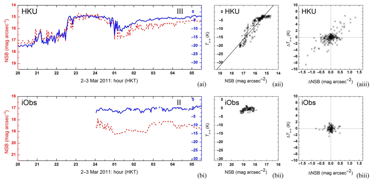
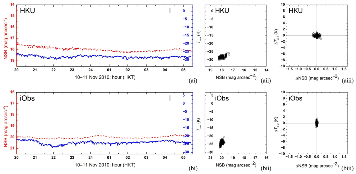
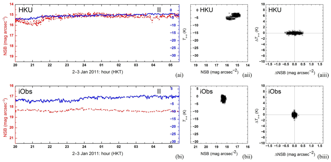
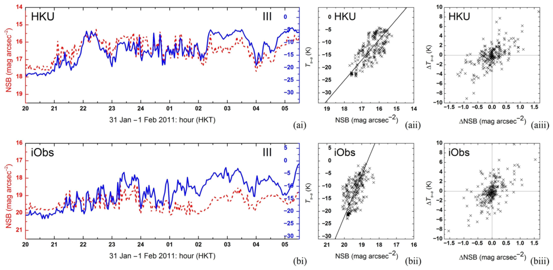
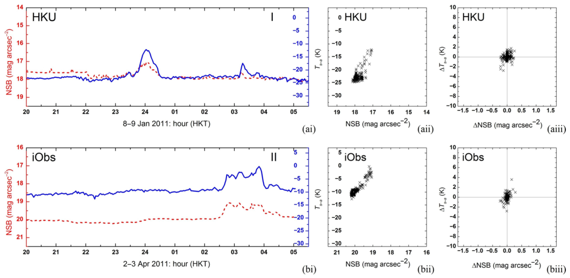
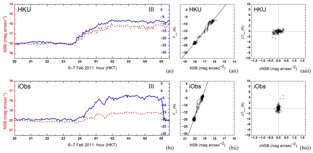
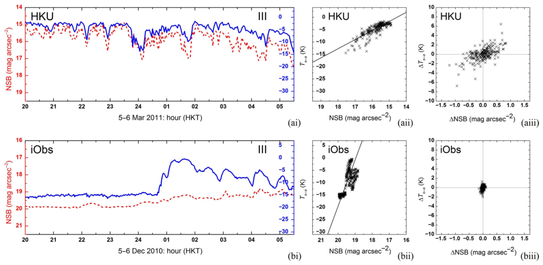
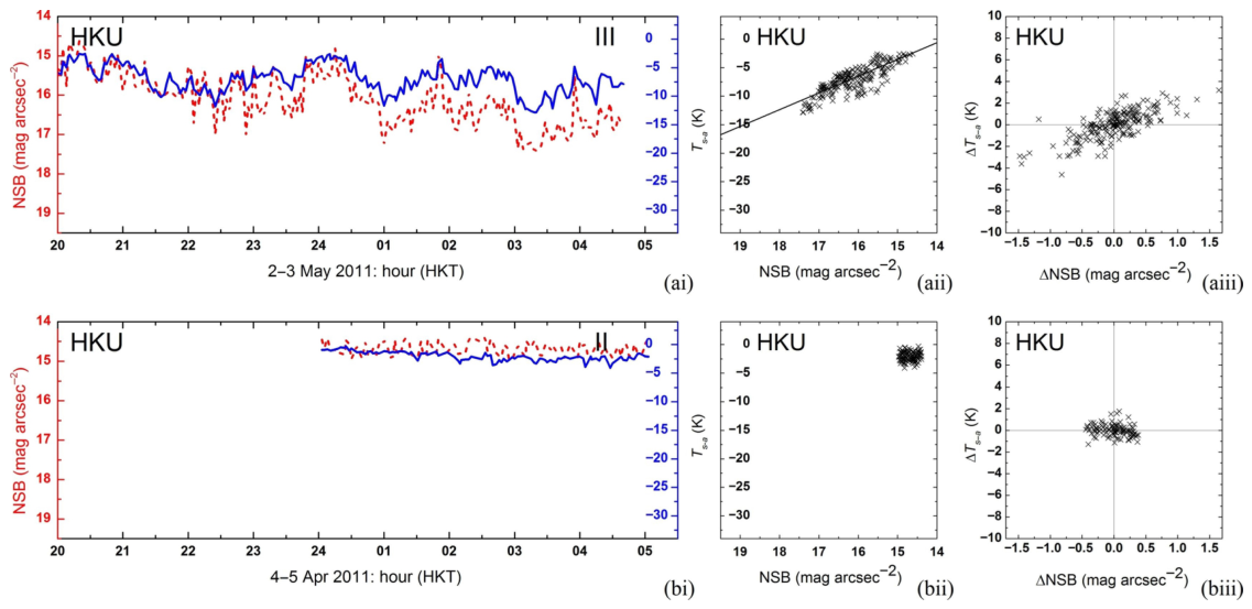
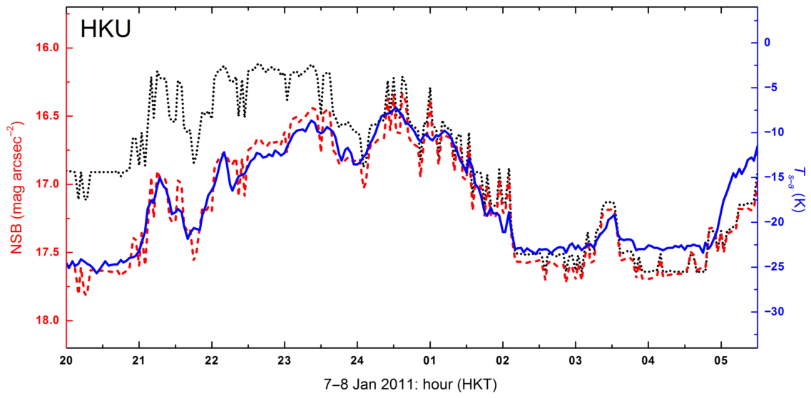
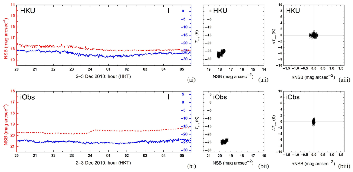
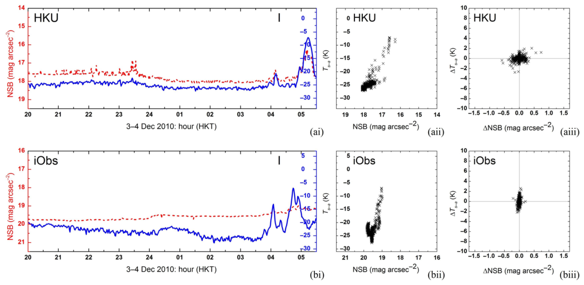
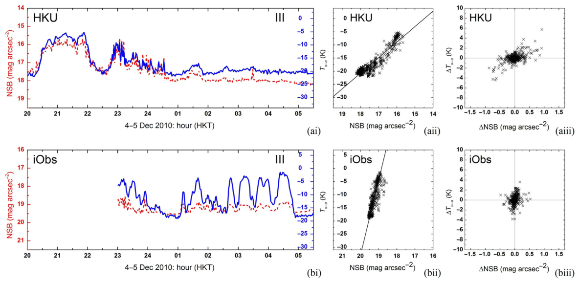
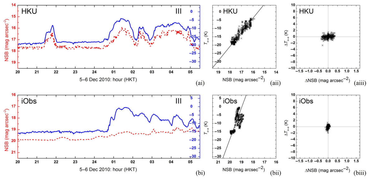
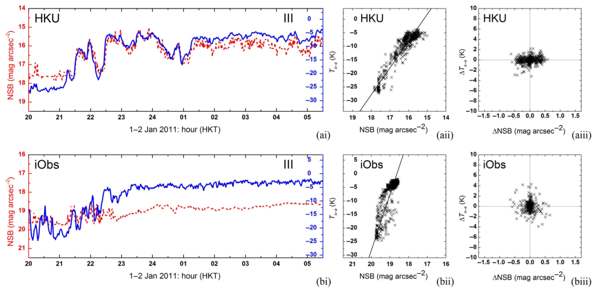
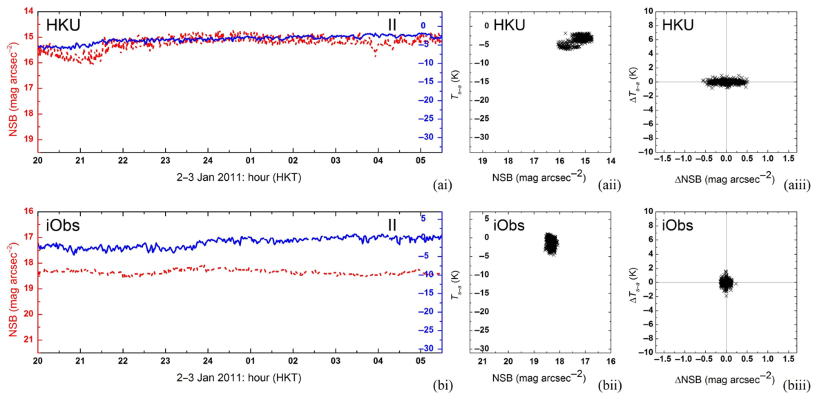
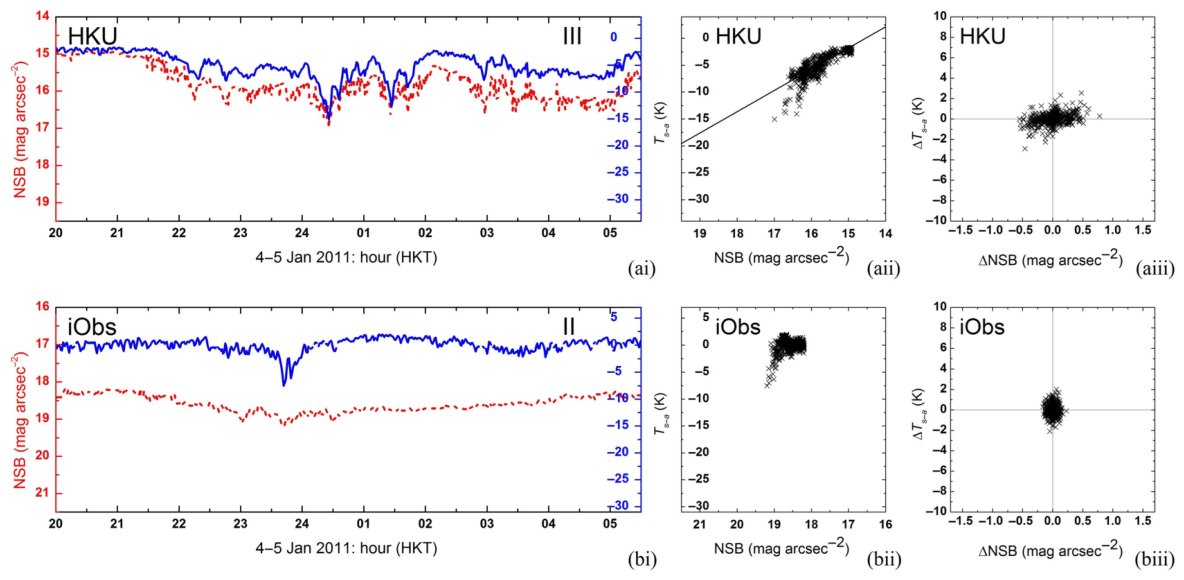
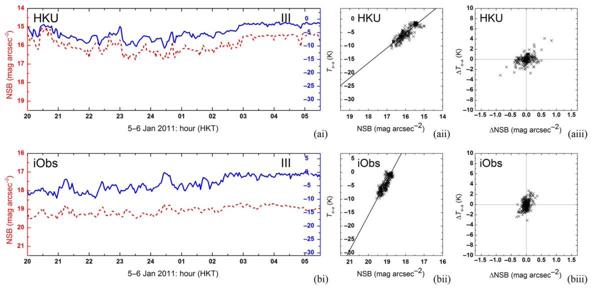
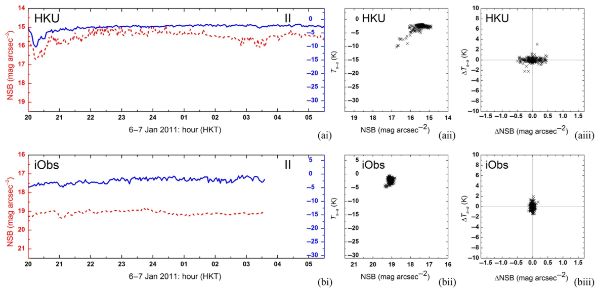
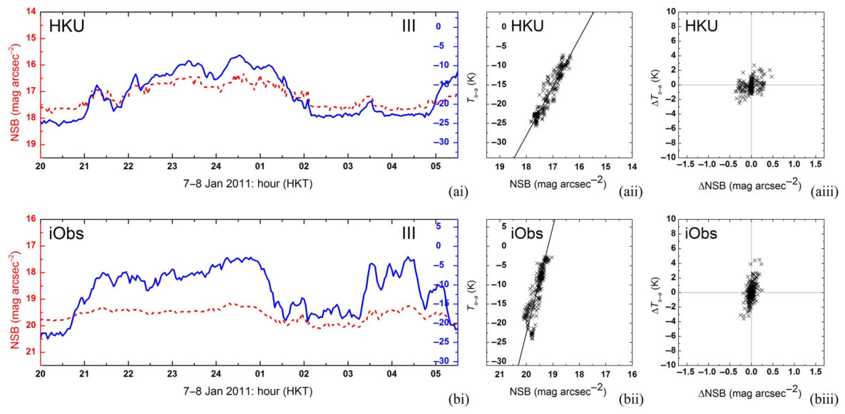
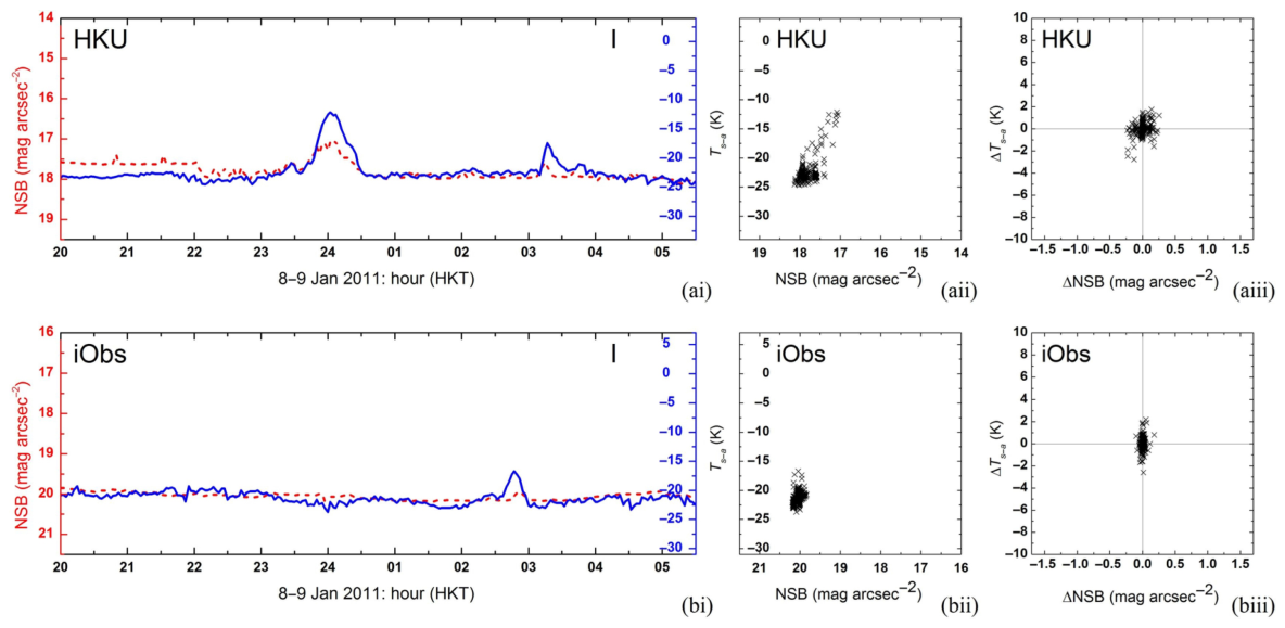
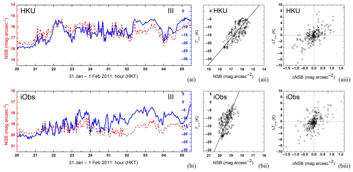
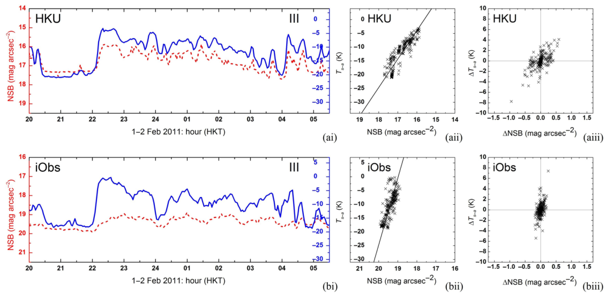
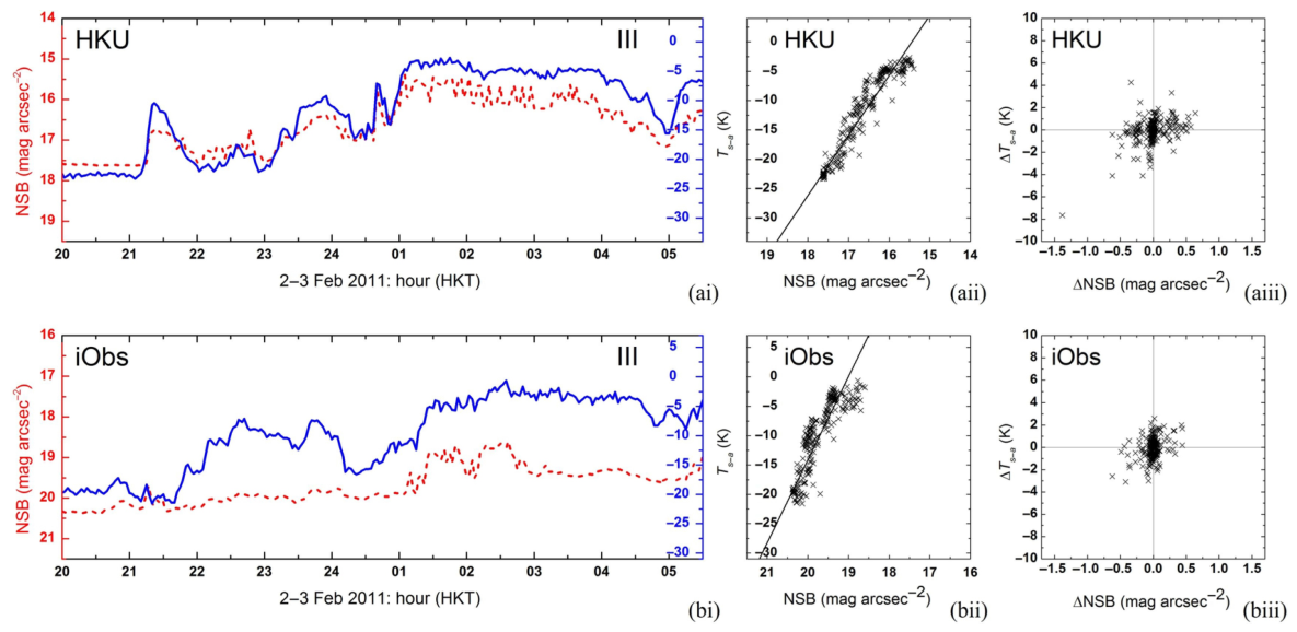
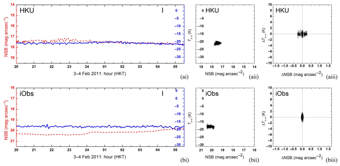
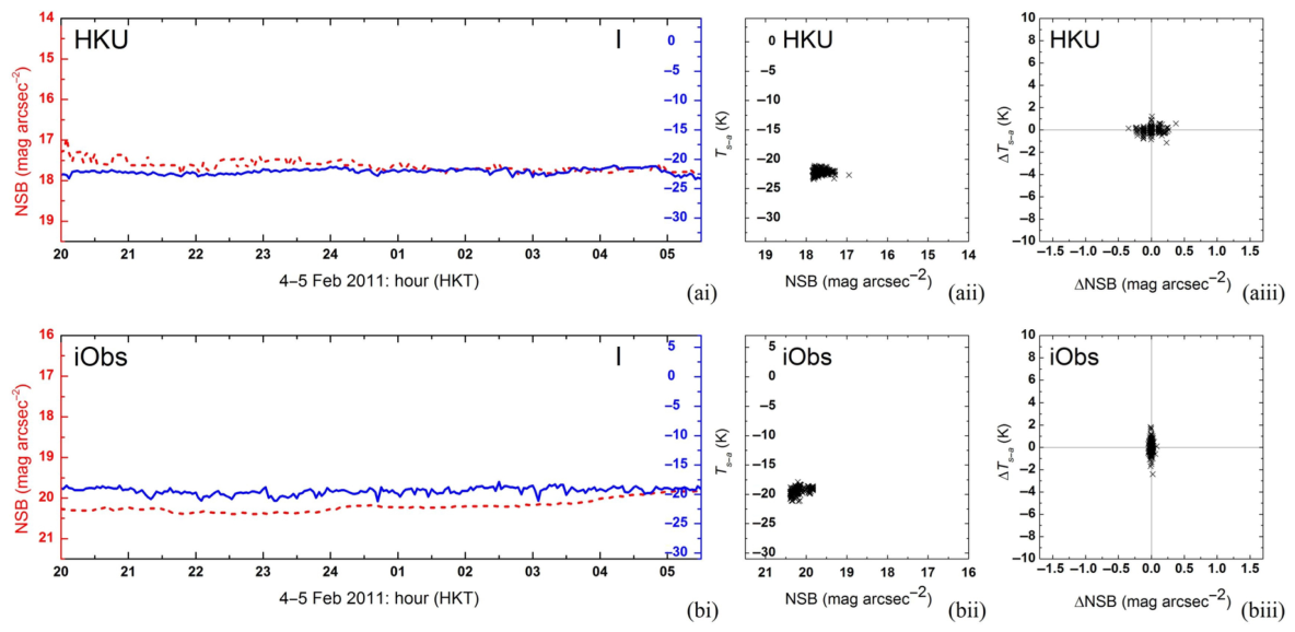
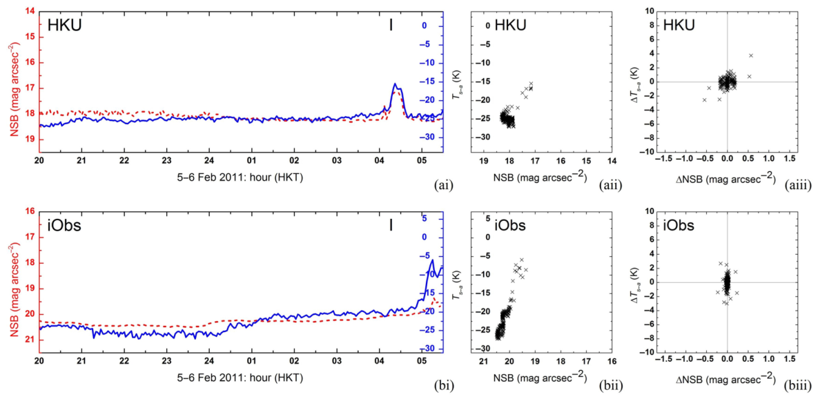
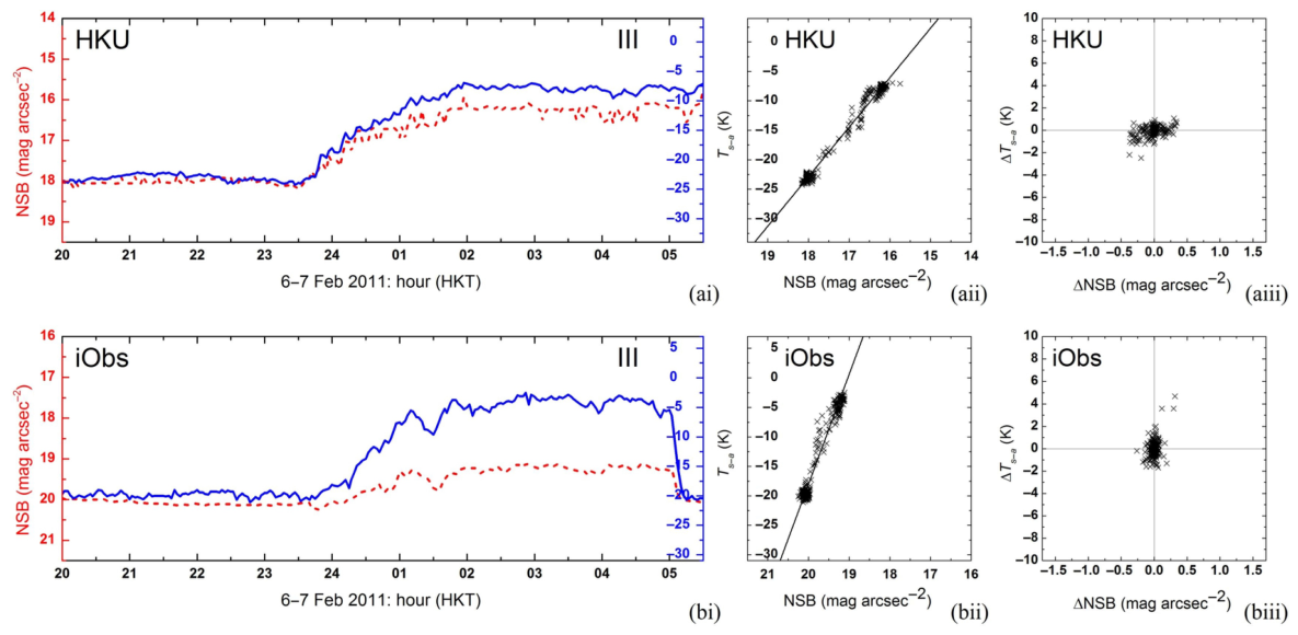
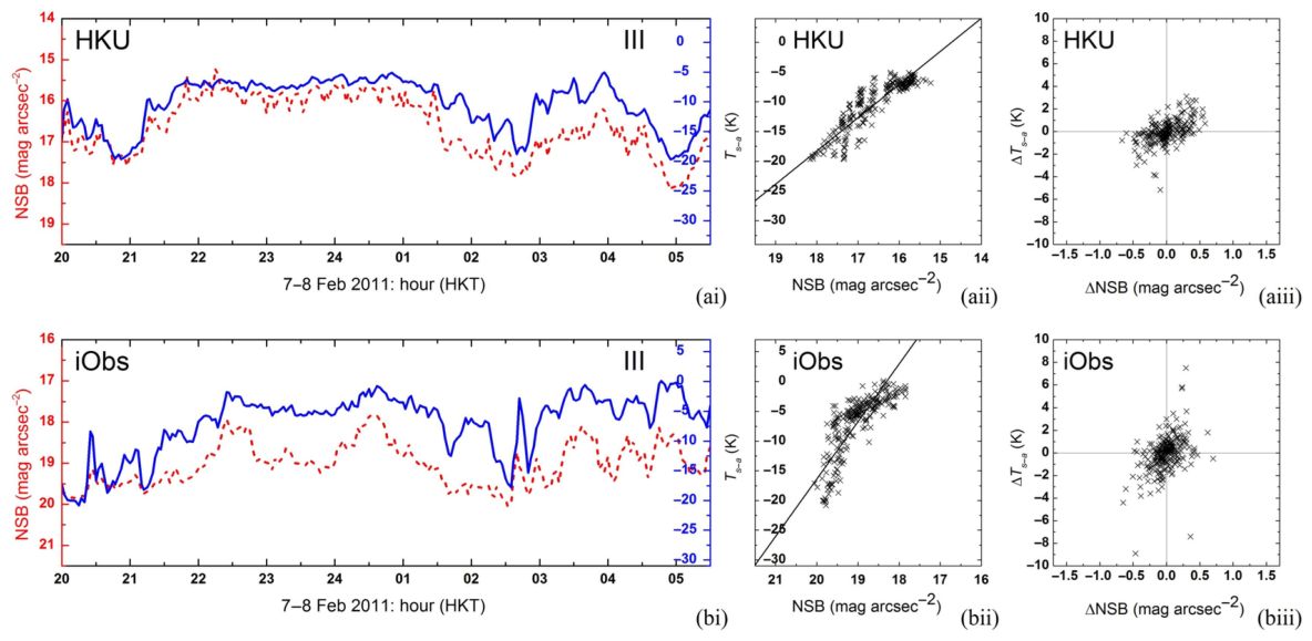
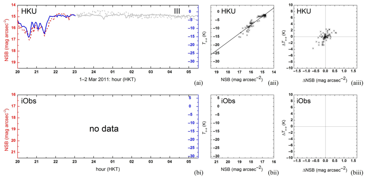
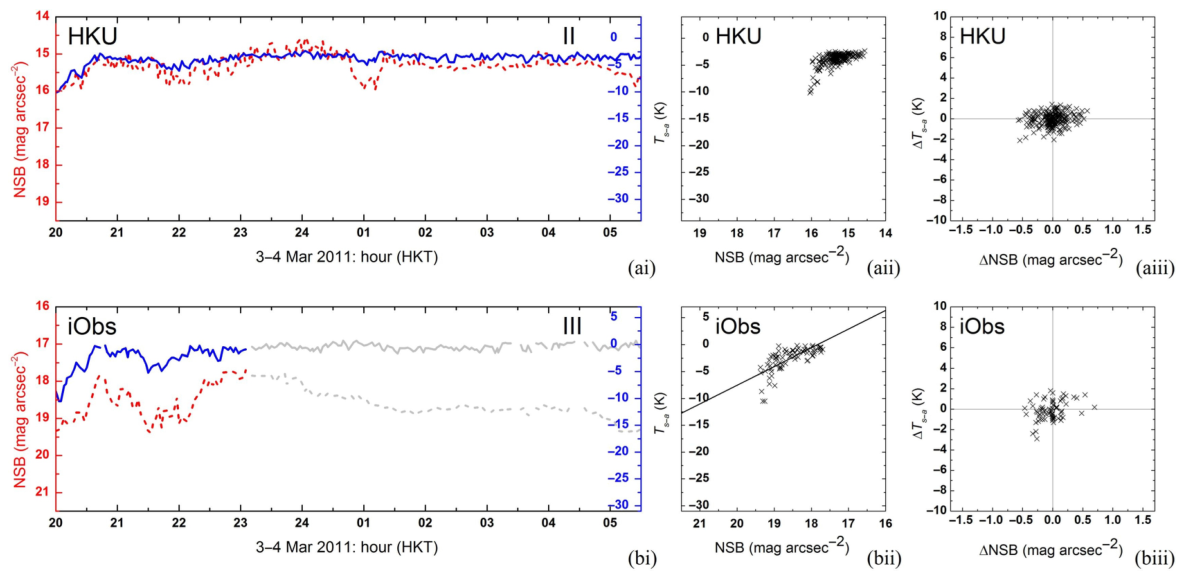
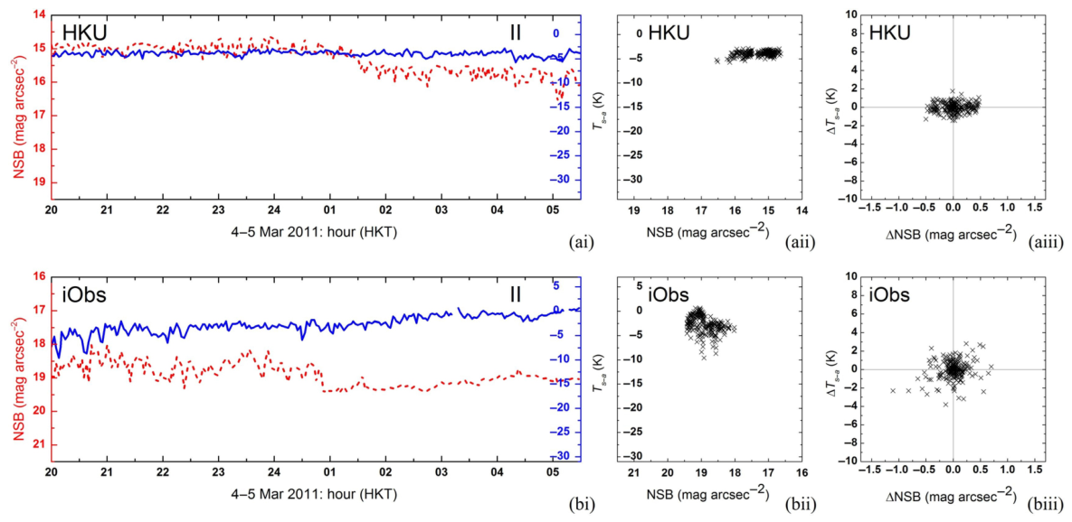
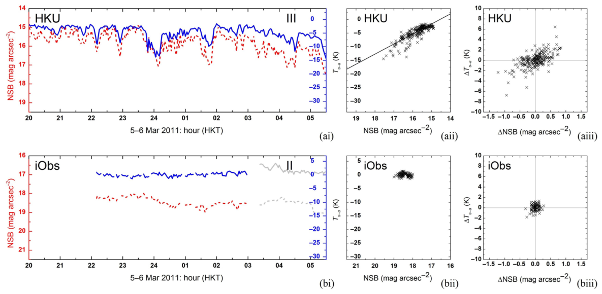
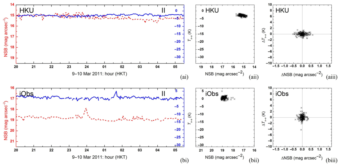
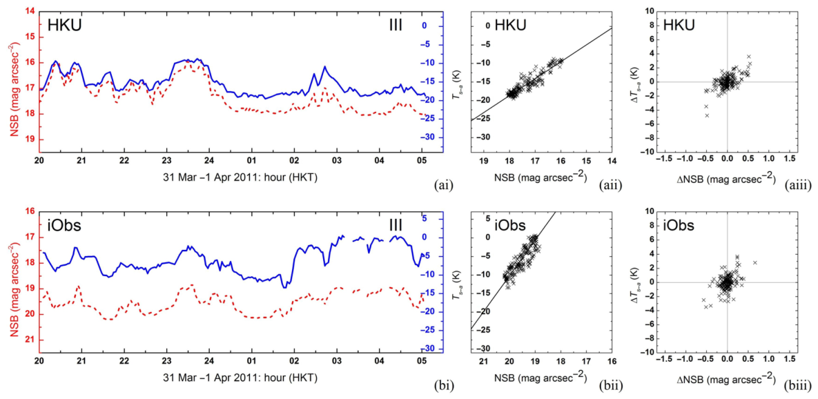
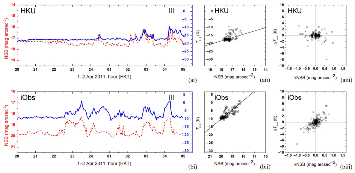
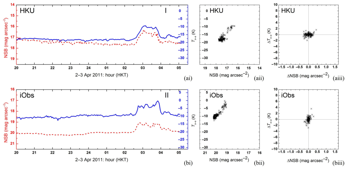
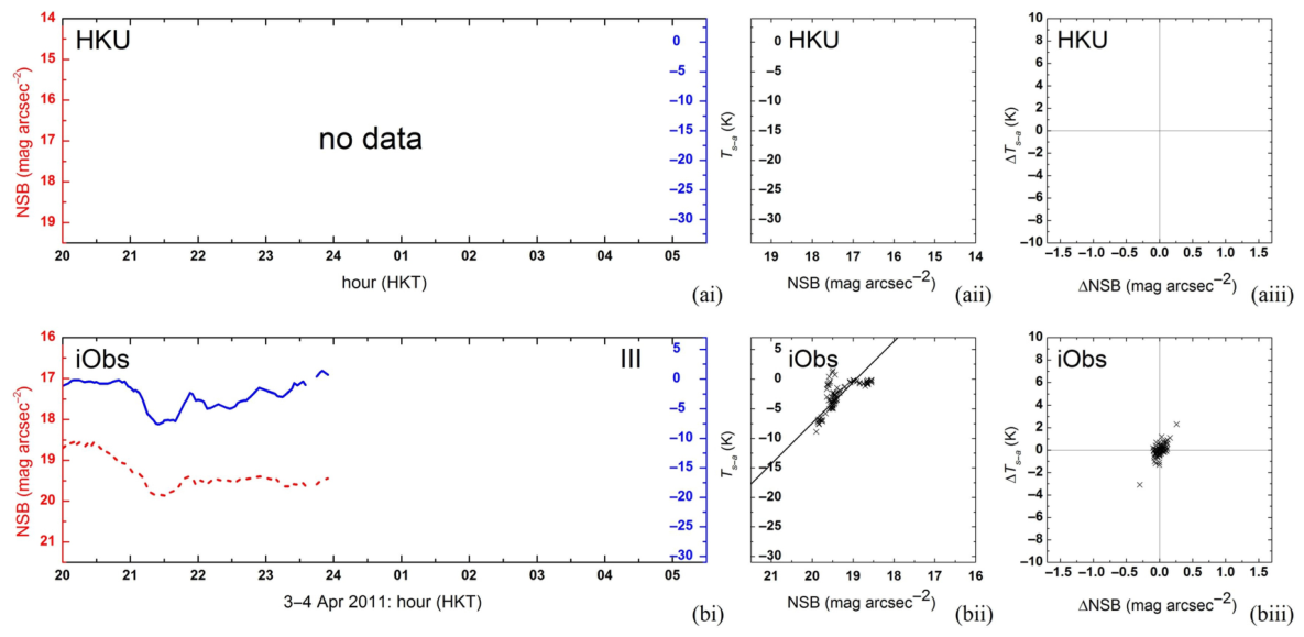
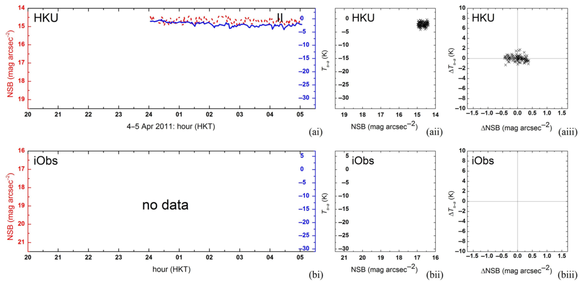
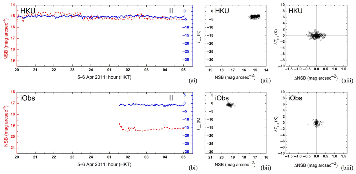
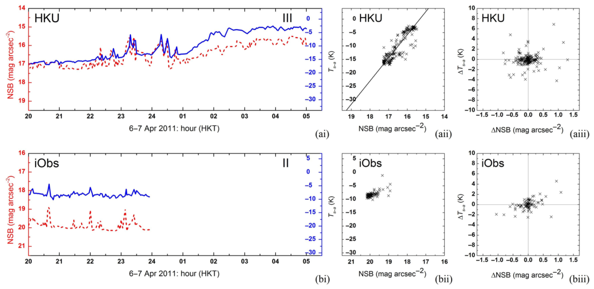
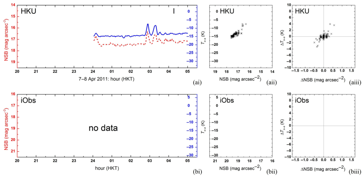
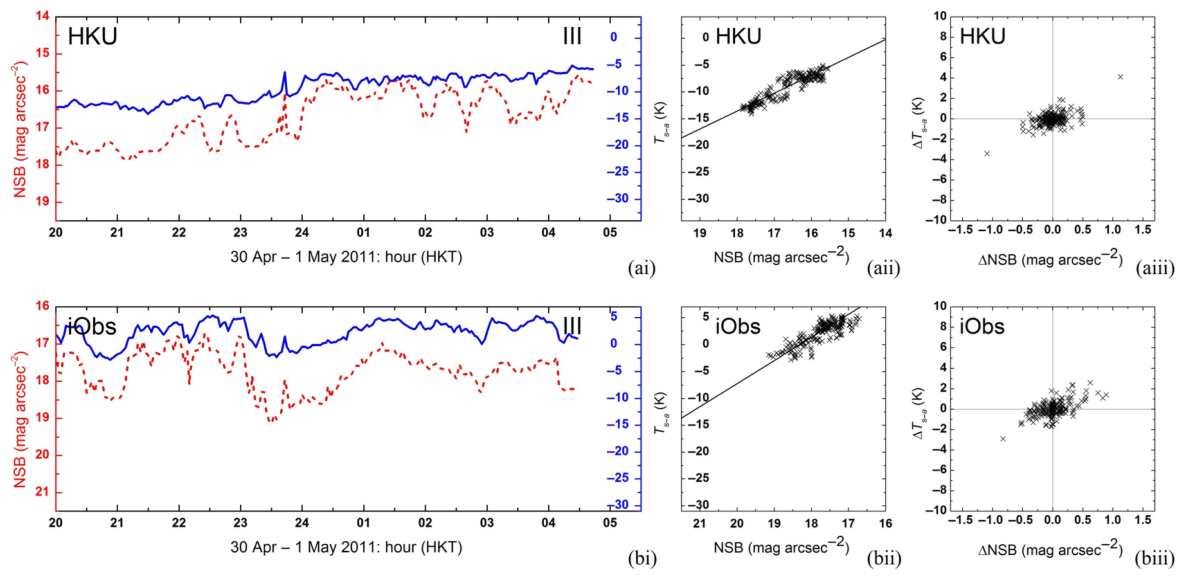
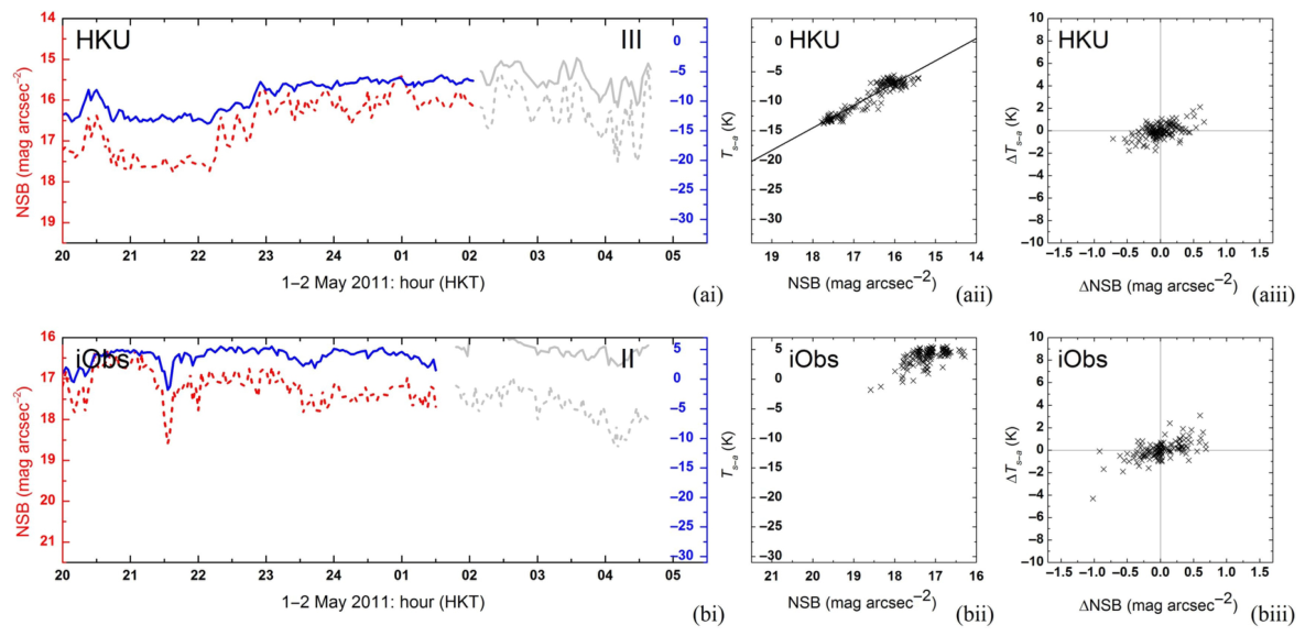
Panels (i) in Figure 13, Figure 14 and Figure 15 show the nightly time series of the NSB and the T s a under typical sky conditions. The complete set of 41 runs is attached in Appendix F. Visual inspection of 41 sets of time series suggests that the sky condition of each run would be classified into one of the three types, according to the variation and level of T s a :
  • Steady Clear Sky (TYPE I): Characterized by a small variation in T s a (small spread of T s a or σ T s a ) with a small level of T s a . Ten (26%) and nine (24%) runs were classified as TYPE I at HKU and iObs, respectively.
  • Steady Overcast Sky (TYPEsII): Characterized by a small variation in T s a (small σ T s a ) with a large level of T s a . Rain droplets were occasionally detected. Seven (18%) and 13 (34%) runs were classified as TYPE II at HKU and iObs, respectively.
  • Diverse Sky (TYPE III): T s a fluctuates dramatically (large σ T s a ) throughout the run, as indicated by a large and prolonged change in T s a . Runs with few occurrences of sudden (less than about an hour) surges in the level of T s a would not be classified as TYPE III (e.g., runs #15-HKU, #33-iObs, see Figure 16). Twenty-two (56%) and 16 (42%) runs were classified as TYPE III at HKU and iObs, respectively.
Columns (5) to (7) in Table A1 and Table A2 in Appendix E list the nightly statistics of T s a (unit: K) and NSB (unit: mag arcsec−2), along with the sky TYPE classifications.
The measured IR T s a value is used to characterize the nighttime cloud amount through broad-type classifications done with mostly visual assessments. In fact, the measured T s a value is most likely a complex atmospheric product influenced by factors not sampled for in our current exploratory study, such as cloud base height and cloud type. Hence, a particular T s a value may represent very different sky conditions in terms of the altitude and emissivity of the cloud layer. Without vertical atmospheric profiles to supplement our data, a fixed threshold might lack the necessary flexibility to account for these environmental variations. In addition, without a well-established theoretical model that connects detailed cloud properties and the observed T s a values, any approach for quantitative classifications would likely be provisional and subject to future refinement.
Nevertheless, our classification is supported by the statistics of T s a and σ T s a , as summarized in Table 4. The data reveals clear trends: TYPE I (clear) and TYPE II (overcast) skies generally maintain a small standard deviation ( σ T s a < 1.5 K), indicating stable atmospheric states. Conversely, TYPE III skies consistently show a larger standard deviation ( σ T s a > 3 K), capturing the inherent fluctuations of variable sky conditions. This synthesis of morphological recognition and statistical consistency provides a grounded classification framework in the absence of established theoretical cutoffs. We conclude that establishing an objective classification threshold is best reserved for subsequent studies when more comprehensive data, particularly on the clouds, are available.
Classifying a sky condition into one of the types is probably a simplification of the real situation. For example, in run #23 (see Figure 17), T s a stays fairly constant at a clear level in the early evening, until a gradual increase in T s a (i.e., clouds rolled in) after ∼23:30. Then, T s a stays fairly constant at an overcast level from ∼02:00 until the end of the observation run. According to this change in cloud amount, that run would be classified as mix-TYPE, with transitions from TYPE I (<23:30) to III (23:30–02:00), and then to II (>02:00). While classifying this run as mix-TYPE would yield a more accurate description, the analysis of the cloud–NSB relationship relies mostly on TYPE III-like data, and the inclusion of non-TYPE-III data within the same run would not significantly affect the analysis. As a result, it was decided that each run would be classified as one of the TYPEs for simplicity.
Nevertheless, a strong correlation between the changes in NSB and the changes in cloud amount can be observed from all sky TYPEs: the sky brightness increases as the amount of cloud rises, and vice versa. In TYPE I runs, the NSB stays steady on a darker level throughout clear nights. In TYPE II runs, the NSB stays steady on a brighter level throughout the overcast nights. In TYPE III runs, the NSB tracks cloud changes closely whenever the cloud amount changes gradually (e.g., runs #23-HKU and #23-iObs; see Figure 17) or suddenly (small patches of cloud rolled in and out, e.g., runs #29-HKU and #07-iObs; see Figure 18). This kind of cloud–NSB relation is defined as a positive correlation. A negative correlation stands for the opposite, i.e., a decrease (increase) in sky brightness with an increase (decrease) in cloud amount.

3.6.2. T s a –NSB

After the classification of sky TYPE, and having a general overview of the cloud–NSB correlation, additional details of the cloud–NSB relationship were revealed by examining the data run by run. The relation between the T s a and NSB measurements (referred to as T s a –NSB hereafter) in each run is presented in the form of scatter plots in panels (ii) of the figures in Appendix F. As can be seen from the figures, the data points from TYPE I and II runs are concentrated in a small region in the scatter plots, as expected. Data points of TYPE III runs exhibit linear distributions in the scatter plots.
To measure the strength of correlation between the change in cloud amount and the change in NSB, the adjusted R 2 , represented by R ¯ 2 , was calculated for each TYPE III run. The results are tabulated in column (8) in Table A1 and Table A2. As can be seen from the Tables, HKU data have a stronger correlation, in which 15 (∼68.2%) runs out of 22 have R ¯ 2 > 0.80 . In particular, the #23-HKU run has the largest R ¯ 2 , at 0.99. Although the data taken during the same run at iObs (i.e., #23-iObs) also has the largest R ¯ 2 at 0.96 for that location, the cloud–NSB correlation is generally weaker at iObs, where only 2 (∼12.5%) runs out of 16 have R ¯ 2 > 0.80 .
To obtain a further quantitative description of the T s a –NSB linearity of the TYPE III runs so that the cloud–NSB correlations could be compared between runs and stations, the Fitexy regression routine described in ([108], Chapter 15) was adopted to fit the data distribution. Given the measurement and instrumental errors (assumed to be uncorrelated) from NSB ( σ x i ) and T s a ( σ y i ), the Fitexy routine accounts for these errors to provide a more accurate representation of the uncertainties in both variables. The fitting results are tabulated in column (9) in Table A1 and Table A2.
An F-test was conducted for each TYPE III run to test the hypothesis of lack of correlation, assuming linearity between T s a and NSB. This test involves the calculation of F probability distribution from the fitting results ([109], Chapter 14). The probability of a lack of correlation is estimated by the size of the p-value. Columns (10) and (11) in Table A1 and Table A2 tabulate the values of F t e s t and p, respectively. As can be seen from the tables, the maximum value of p is only 0.12. As a result, the hypothesis of a lack of correlation can be rejected in all cases. In other words, the cloud–NSB correlations of those runs are highly significant.
The goodness of fit of the linear model was examined by the reduced chi-squared test. The calculated values are tabulated in column (12) in Table A1 and Table A2. The expected value of χ ν 2 for a good fit is 1.0. The fittings from the HKU and iObs runs yield values of χ ν 2 ranging from 0.1 to 6.8, which means that the observations are generally consistent with the assumed linear model. The runs #17-HKU and #12-iObs have values of χ ν 2 equal to 1. The χ ν 2 values of the rest of the HKU runs are all less than 1, while those of all iObs runs are greater than 1, except for two runs. The error variance was most likely incorrectly estimated. One source of error is the cross-calibration of cloud sensors, as mentioned previously in Section 2.2.2.
According to column (9) in Table A1 and Table A2, the slopes of the T s a –NSB fitting not only vary run by run but also vary among locations. The pairwise comparison shows that the slopes in the urban station HKU are larger than those in the suburban station iObs.
The median slope values fitted from all TYPE III runs at HKU and iObs were −5.6 and −15.3 K arcsec2/mag, respectively. If the slope could be interpreted as the measurement of the rate of change in cloud amount as a function of the change in NSB, this implies that a larger change (2.7×) in NSB could be produced by a similar variation in cloud amount in urban locations than in suburban locations in general.
The observed larger change in NSB at HKU can probably be explained by the light pollution conditions in the vicinity of the measurement stations. In an area where external lighting is installed and illuminates the sky directly and indirectly, the sky above that area looks brighter than the natural level because of backscattering of the city light from atmospheric particles. The scattering intensifies when the clouds come in and is weakened when the clouds roll out. There is more external lighting in urban areas, such that the changes in NSB are largely dominated by the variation in the cloud amount. However, there is less external lighting in suburban areas, and the observed changes in the NSB are less affected by the variation in the cloud amount. In sum, urban light pollution at HKU leads to larger fluctuations in NSB.

3.6.3. Δ T s a Δ NSB

As defined in Section 2.2.2 and Figure 2, the location of the data points in the Δ T s a Δ NSB plot represents different cloud–NSB relationships, i.e., how changes in T s a track changes in NSB. Data falling within quadrants I and III have a positive cloud–NSB correlation, in which fewer clouds lead to a dimmer sky or more clouds lead to a brighter sky. However, data falling within quadrants II and IV have a negative cloud–NSB correlation, in which fewer clouds lead to brighter sky or more clouds lead to dimmer sky. Cross-analysis study of Δ T s a Δ NSB is more accurate than that of T s a –NSB, because both Δs are robust parameters independent of the variables’ absolute scale and the transformation of T s a between cloud sensors (Section 2.2.2). Note that the Δ NSB here is different from the Δ NSB late early defined in Section 3.4.
The nightly scatter plot of Δ T s a Δ NSB for each run is shown in panel (iii) in the figures in Appendix F. The percentages of data with a positive correlation are tabulated in column (13) of Table A1 and Table A2 for each run. The highest and lowest figures are 80.0% and 42.7% in runs #41-HKU (TYPE III) and #35-HKU (TYPE II), respectively (see Figure 19). Most of the runs (≥90%) have more than 55% positively correlated data. The percentages of data with a positive correlation ranged from 56.2% to 80.0% for TYPE III runs. The distributions are consistent with their classified sky TYPEs and the cloud–NSB relationships observed previously.
Some of these TYPE III runs—for example, runs #17-HKU and #17-iObs (see Figure 15)—have data points located far away from (0, 0) on the quadrants of positive correlation. These data points represent a large change in NSB (as large as ±1.5 mag arcsec−2 or ∼4× in intensity) caused by a large change in T s a (as large as ±9 K) between two sequence measurements. This feature indicates a very strong cloud–NSB relationship under a rapidly changing sky condition.

3.6.4. ( T s a ) a v g NSB a v g

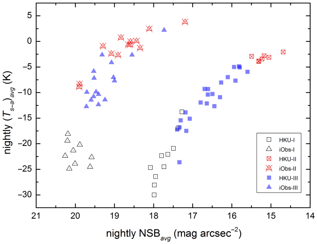
Another way to present the cloud–NSB relationship is shown in Figure 20, where the scatter plots of the nightly averaged T s a , represented by ( T s a ) a v g , and the nightly averaged NSB, represented by NSB a v g , are shown (referred to hereafter as ( T s a ) a v g NSB a v g . The characteristics of the data point distributions for each location include the following: (1) The overall ranges of T s a from the data of all sky TYPEs are different between locations. (2) For each location, the data from different TYPEs are separated in general. Data from TYPE I and II runs populate near the small T s a and large T s a narrow (∼5–10 K in width) regions of the plot, respectively. Data from TYPE III runs are spread in the central broad region (∼25 K in width). However, small portions of data from different sky TYPEs overlap with each other. (3) The distribution of data from all TYPEs in each location is clearly nonlinear. This feature is different from those observed during the run-by-run analysis included earlier in this section, where TYPE III data show linear distributions in the scatter plots of T s a –NSB. The theoretical description of the detailed cloud–NSB relationship is beyond the scope of the present work, but the nonlinearity is possibly related to the relations between unmeasured parameters of cloud properties and actual IR sky radiation received.
One of the potential parameters is cloud base height [110]. Radiation received on the ground from higher clouds should be weaker than that from lower clouds, provided that other factors remain unchanged. Cloud layers with different base heights would lead to different NSB. This kind of relationship was described in [111] and reported in [112]. Ref. [112] observed that the sky was darker when the cloud base was higher, and vice versa. This may explain the difference in the slopes of T s a –NSB in different runs within individual locations, as seen earlier in this section, as well as the large spreads of NSB in Figure 20, where similar values of T s a led to a wide range of NSB if the height of the cloud base varied. It is possible that simultaneous ceilometer (capable of measuring cloud base height) and NSB measurements would help resolve this question, although further investigation may still be needed.

3.6.5. σ T s a σ NSB

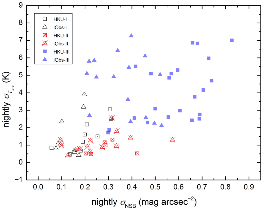
The scatter plot of the nightly σ T s a versus the nightly spread of NSB presented by 1 σ of the spread, or σ NSB (referred to as σ T s a σ NSB hereafter), in Figure 21 supplements the description of the cloud–NSB correlation, as discussed earlier in this section. In HKU, there is a general trend that a larger spread in T s a causes a greater spread in NSB, and vice versa. For TYPE III, although both stations have roughly the same extent of σ T s a , the extent of σ NSB at iObs is much smaller than that of HKU. This discrepancy could be explained by light pollution conditions in the vicinity of the measuring stations: the increase in cloud brightness in the suburban area is smaller than that in the urban area under the same cloud conditions because less external lighting is installed and illuminating the sky directly and indirectly in the suburban area. Therefore, the overall spread of NSB observed in suburban areas is smaller. This is similar to the explanation for the difference in T s a –NSB linearity among stations earlier in this section.

3.6.6. Statistics of Cloud–NSB Correlation

Table 5 tabulates the statistics of positive and negative cloud–NSB correlations in each location. Statistics for all data and for only the TYPE III data were calculated separately. As shown in the table, positive correlations dominate at both locations, consistent with the expectation that clouds brighten the night sky in areas affected by light pollution. The percentages of data with a positive (negative) correlation are slightly increased (decreased) after removing TYPE I and II data. As shown in the last part of the table, about 84% of the data points are positively correlated in each location, although the sample size reduces significantly, if TYPE III data inside the ranges of natural fluctuation—which are Δ T s a 1 K and Δ NSB 0.25 mag arcsec−2, as determined from data distributions—are further removed. The distributions of the last kind of data subsets are visualized in Figure 22 and Figure 23.
Approximately 16% of data points fall into the negatively correlated quadrants (II and IV). At truly dark locations, quadrant II would correspond to starlight brightening the unclouded sky, while quadrant IV would represent clouds darkening the sky by shielding starlight. However, since our observations were conducted in light-polluted locations, the presence of data in quadrant II or IV reveals that the cloud–NSB relationship is imperfect. These counterintuitive cases could arise from factors such as variations in cloud type, altitude, thickness, or local ground lighting conditions. Future work comparing these findings with measurements from a truly rural, light-free site would help disentangle the relative contributions of artificial versus natural light sources to the observed cloud–NSB correlation.

3.6.7. Cloud–NSB Correlation Beyond Natural Fluctuation

Least-squares linear regressions were conducted on the last kind of distributions by the Fitexy routine ([108], Chapter 15). The slopes (weighted by errors in both variables) of the best-fit straight lines are 3.2 ± 0.4 ( F t e s t = 495.0 , p-value = 0.04, χ ν 2 = 0.1) and 5.0 ± 0.2 K arcsec2/mag ( F t e s t = 296.3 , p-value = 0.05, χ ν 2 = 1.2) for HKU and iObs, respectively.
The best-fit slopes of Δ T s a Δ NSB carry the same meaning as the nightly slopes obtained from the T s a –NSB scatter plots earlier in this section: the measurement of “sensitivity” of NSB responds to changes in cloud amount under different light pollution conditions. The smaller slope obtained at HKU implies that the night sky in urban areas is more “sensitive” to the variation in cloud amount—a consequence of excessive use of artificial lighting in urban regions. This property is consistent with the cloud–NSB relations observed previously. As discussed earlier in this section, the analysis conducted here does not suffer from calibration issues, since Δs are independent of the variables’ absolute scale.

4. Discussion

Building upon the earlier NSB monitoring projects, a more comprehensive sky light pollution study was conducted for Hong Kong from NSB data collected between May 2010 and June 2023. The monitoring allowed us to understand the long-term changes in light pollution in the region. In particular, the observation periods for four urban locations and two suburban locations spanned ten years. We revealed that the moonless night skies in Hong Kong were 43× brighter than the dark sky standard set by the IAU in 2014–2023. Urban locations were found to be nearly 120× brighter than the dark sky standard, while suburban locations were around 10× brighter. The urban and suburban locations differed by around 10×. This study also found that, among the monitored areas, King’s Park and Tsim Sha Tsui in Kowloon had the brightest night sky, while Sai Kung Country Park and Cape D’Aguilar in Shek O were the darkest locations monitored. Nightly variations in the NSB were explored, revealing that the early-evening skies were generally brighter than the late-night skies due to the presence of more external light before midnight. Monthly variations in NSB were also analyzed, indicating that NSB varied seasonally in different years. This variability was attributed to varying cloud amounts, which have been shown to affect NSB. Over the study’s duration, the overall brightness of the Hong Kong night sky was relatively steady.
When comparing the situation a decade ago (May 2010–March 2013) with that presented in [15], we introduced the robust indicator Δ NSB late early , which is relatively unaffected by instrumental variations or systematic errors. This analysis revealed that urban areas were darker over the decade, characterized by lower after-midnight NSB levels and a more extensive degree of darkening post-midnight. The changes can be attributed to multiple factors, including economic considerations and improved awareness of light pollution reduction, promoted by external lighting guidelines, particularly the Charter on External Lighting [99]. The study period overlapped with the COVID-19 pandemic (early 2020–mid 2023) and two solar cycles (Cycle 24: 2008–2019; Cycle 25: since December 2019). Additional data and further analysis are needed to disentangle the complex interplay of economic and natural factors.
With the measurements of Δ NSB late early , this ground-based study provides a unique approach to directly assess the impact of ALAN within a small area and a single night, capturing light pollution conditions that are not reflected in nighttime satellite imagery, which is commonly constrained by sparse spatial resolution, infrequent overpass times, cloud contamination, poor-quality observations, and “blue-blindness” [37]. With advancements in instrumentation (e.g., higher sensor spatial resolution [113,114,115,116]) and techniques (e.g., integrating different data sources with different overpass times [117,118]; characterizing ground-based light sources from nighttime satellite imagery [119]; data gap-filling [120]) for space-based remote sensing of night lights, ground-based observations not only serve as essential validations for satellite data but also pave the way for new discoveries in our understanding of light pollution dynamics.
It is well established that the presence of clouds affects NSB observations. Particularly, cloudy skies are brighter because of backscattered ALAN from the ground, and vice versa. Unlike previous studies on the impact of clouds on NSB, primarily based on sparse okta-scale cloud observations, this study, for the first time, obtained cloud amount data more precisely, based on the IR sky–ground temperature difference. Using more than 640 h of simultaneous NSB and cloud amount observations, we quantitatively investigated the cloud–NSB relationship in urban and suburban settings. Our results confirm that the cloud amount is a key factor in determining short-term fluctuations in NSB. We observed a strong correlation ( R ¯ 2 up to 0.99) between changes in cloud amount and changes in NSB, whereby an increased cloud amount leads to a brighter sky, and vice versa. Due to light pollution, urban areas exhibited nearly three times greater changes in NSB than suburban areas for comparable changes in cloud amount. Our results also revealed that the cloud–NSB relationship is imperfect, highlighting the need for further research on the cloud–NSB relationship, including how NSB changes with cloud base heights and cloud types.
The findings also highlight a critical ecological vulnerability: the dramatic amplification of skyglow under cloudy conditions. Many nocturnal species are highly sensitive to anthropogenic light, often suffering habitat loss or behavioral disruption. For example, the critically endangered Oculogryphus chenghoiyanae—a firefly species endemic to Hong Kong—was found to have vanished from its known habitat after the installation of high-intensity street lighting along its primary paths [121]. Even subtle increases in ambient light intensity can be equally detrimental; another local species, Pteroptyx maipo, has been shown to cease flashing in response to minor elevations in light levels [122]. Since our data indicate that cloud cover can significantly amplify skyglow, such atmospheric conditions may inadvertently push ambient light beyond the threshold for these species, creating a behavioral shift that directly threatens reproductive success and greater biodiversity [121]. These cases illustrate that the cloud-amplification effect does not merely obscure the stars but poses a tangible threat to the survival of Hong Kong’s unique nocturnal fauna.
Our study has some limitations that should be considered.
First, over the past decade, lighting technology has undergone a significant transition from traditional sources, such as high-pressure sodium and incandescent lamps, to solid-state lighting (e.g., LEDs). Because LEDs generally exhibit higher blue-light content, and the SQM sensors used in this study are less sensitive to the blue end of the spectrum, the sensors may not fully account for the spectral shifts associated with this technological transition. This discrepancy is well documented in the literature [13,18,37,53,123,124,125], suggesting that the observed darkening trends may require further quantification to validate. Our recent studies have addressed this shortcoming by observing sky spectra, allowing for a more detailed analysis of light pollution [126]. By examining the specific wavelengths of light emitted in the night sky, we can identify the sources of light pollution more accurately. This approach enables us to differentiate between various types of lighting, such as streetlights, commercial advertisements, and residential lights, each of which contributes differently to the overall brightness of the sky.
Second, the sensor used to measure skyglow is designed to detect brightness at the zenith, the highest point in the sky. However, the sensor’s sensitivity drops significantly, by a factor of 100, when measuring light sources that are ∼40° or more away from the zenith, as reported in [76]. This means that the sky brightness estimates obtained from this type of sensor may not accurately represent the impact of ALAN from sources near the horizon, such as billboards and TV wall panels designed to illuminate horizontally. To improve this, future studies may consider deploying wide-field or all-sky cameras, which can record emissions from more or all directions, as successfully demonstrated in the literature [13,23,24,25,127,128]. On the other hand, because low-angle light emissions are most important at distant sites due to multiple scattering [129,130], establishing additional monitoring stations farther from Hong Kong would be beneficial. This would strengthen our understanding of the behavior of urban and suburban locations in this study.
Third, the instrumental configuration for the NSB observations used in this study experienced changes in the type of sensor housing window over time. Some sensors were equipped with light shields to block direct stray light. In addition, there have been declines in the efficiency of light sensors and the throughput of the protective window over the past decade. As described in Section 2.2.1 and [39], we accounted for these changes using empirically determined offset values. However, the actual effects may be wavelength-dependent and were difficult to model precisely over a long period of time. Nevertheless, even though individual NSB observations may have been subject to uncorrected uncertainties, the results of the before- and after-midnight comparisons presented in Section 3.4 remain robust. This robustness was ensured as long as our comparisons were conducted within individual nights (Figure 10), where instrumental uncertainties were effectively eliminated.
Fourth, the NSB statistics and the geographic and temporal variations presented in the analysis are inherently biased due to uneven sampling across different time periods and locations. The sampling was primarily restricted to late-night hours and winter seasons, when the duration of night is longer. Additionally, older monitoring stations have accumulated more data over time compared to newer stations (Table 1 and Table 2). This uneven sampling across both temporal and spatial dimensions means that the reported statistics and trends may not be fully representative of the overall NSB conditions throughout the year or across all monitoring locations.
Fifth, the cloud observation method did not distinguish between varying cloud base heights, cloud types, and optical thicknesses, or high cirrus composed of ice crystals. Additionally, we did not measure the spatial distribution of cloud coverage or the partial cloud amount (the extent of sky covered by each type or layer of clouds). Inspired by recent studies [53,57], investigating the relationships between these additional cloud properties and NSB at different wavelength ranges will be essential for future research. We further recommend angularly resolved (e.g., with calibrated all-sky cameras) and ceilometer (capable of measuring cloud amount at different heights) measurements for future studies aimed at characterizing the non-uniform illumination of clouds by ALAN.

5. Conclusions

The natural night sky—often regarded as a shared heritage of humanity [6]—is increasingly threatened by ALAN. Our analysis reveals that light pollution is pervasive across Hong Kong, characterized by stark contrasts between urban and suburban environments. Crucially, our decade-long data indicate a policy-relevant shift: urban areas have become measurably darker over the past ten years, with more pronounced post-midnight dimming in city centers. This trend suggests that improved compliance with lighting regulations and voluntary guidelines carries positive implications for reducing light pollution in densely populated areas.
Specifically, we propose several actionable recommendations aimed at maximizing mitigation efficiency:
  • Stringent Lighting Policies: Given the effectiveness of post-midnight dimming observed in our data, existing policies, including the Charter, should be strictly maintained to ensure that non-essential decorative and commercial lighting is switched off at preset times. To achieve more consistent results, future policy should consider transitioning from voluntary agreements to mandatory legislative requirements. This would include standardized curfews for high-intensity signage and the implementation of dynamic dimming protocols, where illumination levels are automatically reduced during late-night hours or low-traffic periods to minimize unnecessary skyglow while maintaining public safety.
  • Mandatory Shielding: Due to atmospheric scattering, cloudy nights are much brighter when unshielded light is most aggressively reflected back to the surface. Given that a small number of intense sources contribute disproportionately to urban skyglow [25,115], regulations should mandate the use of full-cutoff fixtures to eliminate all direct upward light emission. Furthermore, future requirements should extend beyond simple shielding to include strict tilt-angle restrictions for all external lighting fixtures, ensuring that light is confined strictly to the intended target areas and does not contribute to the scattered light that disrupts the sky and local ecosystems.
  • Enhancing Public Awareness and Engagement: While policy and technical fixes are vital, long-term success requires fostering a culture of dark sky conservation. Authorities should leverage our data and findings to launch public education campaigns that highlight the ecological and health benefits of dark skies, specifically targeting residents and business owners. Initiatives such as citizen science monitoring programs or public stargazing events can reconnect urban populations with their natural heritage. By increasing transparency and accessibility of real-time light pollution data, the public can be empowered to make informed choices, thereby transforming the protection of the night sky into a collective community priority.
Our findings demonstrate that practical solutions are within reach if motivated and implemented thoughtfully. Sustained, localized NSB monitoring can help track progress and inform evidence-based policy. Together with advances in remote sensing and public participation, behavioral and policy changes can drive light trespass reduction and energy savings. Protecting the night sky will therefore yield co-benefits for ecology, public health, energy efficiency, and the cultural value of stargazing for future generations.

Author Contributions

Conceptualization, C.W.S. and C.S.J.P.; methodology, C.W.S. and C.S.J.P.; software, C.W.S. and S.L.; validation, C.W.S., C.S.J.P., and S.L.; formal analysis, C.W.S. and S.L.; investigation, C.W.S.; resources, C.W.S. and C.S.J.P.; data curation, C.W.S.; writing—original draft preparation, C.W.S.; writing—review and editing, C.S.J.P. and S.L.; visualization, C.W.S.; supervision, C.S.J.P.; project administration, C.S.J.P.; funding acquisition, C.S.J.P. All authors have read and agreed to the published version of the manuscript.

Funding

This research was funded by the Environment and Conservation Fund (Project IDs: 2009-10, 125/2018, 113/2022) of the Government of the Hong Kong Special Administrative Region. Any opinions, findings, conclusions, or recommendations expressed in this article do not necessarily reflect the views of the Government of the Hong Kong Special Administrative Region and the Environment and Conservation Fund. The Globe at Night—Sky Brightness Monitoring Network (GaN-MN) is co-organized by the Office for Astronomy Outreach of the International Astronomy Union (IAU-OAO), the University of Hong Kong (HKU), the National Astronomical Observatory of Japan (NAOJ) and Globe at Night. The Globe at Night citizen science campaign to monitor light pollution levels worldwide is hosted by the U.S. National Science Foundation National Optical-Infrared Astronomy Research Laboratory (NSF NOIRLab). GaN-MN was funded by the HKU Knowledge Exchange Fund granted by the University Grants Committee (Project No.: KE-IP-2014/15-57, KE-IP-2015/16-54, KE-IP-2016/17-44, KE-IP-2017/18-54, KE-IP-2018/19-68, KE-IP-2019/20-54 and KE-IP-2020/21-78), IAU-OAO and NAOJ.

Data Availability Statement

Raw NSB data required for replication are available at https://globeatnight.org/gan-mn/ (accessed on 25 April 2026). Other data will be available on request.

Acknowledgments

We collaborated with different organizations to establish and run NSB monitoring stations outside HKU’s properties in recent years. They include the Hong Kong Space Museum (TST, AP and iObs), the Ho Koon Nature Education cum Astronomical Centre (Sponsored by Sik Sik Yuen) (HKn), Hong Kong Observatory (KP, SH2 and Cap2), and Fanling Kau Yan College (FKYC). Their assistance is highly appreciated.

Conflicts of Interest

The authors declare no conflicts of interest.

Abbreviations

The following abbreviations are used in this manuscript:
ALANArtificial Light At Night
FOVField of View
FWHMFull Width at Half-Maximum
GaN-MNGlobe at Night—Sky Brightness Monitoring Network
HKIHong Kong Island
HKOHong Kong Observatory
IAUInternational Astronomical Union
IRInfrared
KLNKowloon
LEDLight-Emitting Diode
LILantau Island
NSBNight Sky Brightness
NSNHong Kong Night Sky Brightness Monitoring Network
NTNew Territories
SQMSky Quality Meter
SQM-LESky Quality Meter–Lens Ethernet
TESS-WPhotometer–Telescope Encoder and Sky Sensor
UTCCoordinated Universal Time

Appendix A. Cross-Check Experiments of Two Cloud Sensors

During the cross-check experiments, two sensors were placed side by side at ∼0.2 m apart. Based on this setting, it was assumed that both devices were measuring essentially the same piece of sky under identical environmental conditions. The first experiment was conducted at HKU during 6 to 13 December 2010, while the second experiment was conducted at iObs during 17 to 20 December 2010. A total of ∼201,000 and ∼72,000 raw data entries for T s a , covering a wide temperature range, were collected at the two locations, respectively. To compare the absolute data scales between the two sensors, the measured T s a values from both experiments are plotted in Figure A1 and Figure A2.
The distribution of data points suggests a linear relationship. The least-squares linear regression conducted on all data collected from both locations indicated a strong positive correlation ( R 2 = 0.98 ) between the readings of the two sensors. Significant F-test results from a one-way ANOVA at a 5% alpha level reveal that the linear regression fitting has a p-value of 0. The straight lines in Figure A1 and Figure A2 represent the best fit. However, the fitted line deviated from the 1:1 relation. In particular, cloud sensor 1 consistently gave larger T s a readings under the same sky conditions, which is not surprising, as the manufacturer did not provide the absolute sensitivity and responses of the detectors. Possible reasons behind this discrepancy include the following [131]: (1) two sensors having slightly different electronics and/or firmware; (2) the thermopile of one of the sensors being older than the other (sensor degrades over time); (3) the humidistat located at the bottom of the sensor for T a measurements reading different temperatures due to variations in manufacturing and local airflow; and (4) one sensor “saw” the other, but not vice versa, during the side-by-side cross-check experiments, such that the IR radiation generated by the electronics of one of them was detected by the thermopile of another if they were mounted closely. Note that the angular acceptance cone of the IR sensor is unknown.
Figure A1. Correlation of T s a measured by two cloud sensors during the cross-check experiment conducted at HKU. Distribution of data points is represented by relative density. The solid line is the best linear fit of all data collected from HKU and iObs. The dashed line represents a 1:1 relation.
Remotesensing 18 01691 g0a1
Figure A2. Same as Figure A1 for the experiment conducted at iObs.
Remotesensing 18 01691 g0a2
Since it was uncertain which sensor provides the most accurate T s a readings, for a quantitative comparison of the difference in cloud amounts between stations, the T s a values measured from cloud sensor 2 were transformed to those of sensor 1 to correct the discrepancies in the measuring equipment. The transformation was conducted by applying the following fitted linear relation:
T s a , s e n s o r 1 = 0.71 × T s a , s e n s o r 2 + 1.1 .

Appendix B. Removal of Nightly Temporal Variations in NSB Due to Artificial Light for Cloud–NSB Analysis

The effect of nightly temporal variations in NSB due to artificial light was removed prior to the cloud–NSB analysis according to the method described in [39] (Section 3.3.1.1). In summary, using the average NSB at 04:30 ( M ( 04 : 30 ) ) observed at each location during the NSN study period as a baseline, the NSB records M ( t ) at time t were offset with Δ M ( t ) = M ( 04 : 30 ) M ( t ) . Figure A3 shows an example of the HKU light curve before and after correction. Before the correction, the light curve has two forms of cloud–NSB relationship across the early evening and late night, in which the light curve after midnight tracks the variation in cloud amount better than that before midnight. After the correction, the NSB shifts to the dark end, with a larger correction in the early evening, such that the light curve tracks the variation in the cloud amount very well throughout the entire night. The correction plays an essential role in revealing a homogeneous cloud–NSB relationship for the entire run.
Figure A3. Example of the NSB light curve at the urban station HKU before (black dotted curve, left axis) and after (red dashed curve, left axis) the correction for the nightly temporal variations in NSB due to artificial light. Cloud amount, measured in T s a (blue curves, right axis), is overlaid for comparison.
Remotesensing 18 01691 g0a3

Appendix C. Plots of Long-Term Time Series of NSB Observed at Other Locations

Figure A4. Average sunlight- and moonlight-free early-evening (before 22:00 in red) and late-night (after 01:00 in green) NSB variations observed at KP every month. The red and green bars represent the monthly sample sizes for the early-evening and late-night datasets respectively, which show seasonal variations due to sunlight cutoff. Key offline events, if any, are labeled on the time series.
Remotesensing 18 01691 g0a4
Figure A5. Same as Figure A4 for TST. The y-axis scale is different from others.
Remotesensing 18 01691 g0a5
Figure A6. Same as Figure A4 for FKYC. Before September 2022, the sensor was battery-powered, which led to incomplete sampling whenever the battery ran out.
Remotesensing 18 01691 g0a6
Figure A7. Same as Figure A4 for HKn.
Remotesensing 18 01691 g0a7
Figure A8. Same as Figure A4 for iObs.
Remotesensing 18 01691 g0a8
Figure A9. Same as Figure A6 for Cap2.
Remotesensing 18 01691 g0a9

Appendix D. Simplified Plots of Monthly Time Series of NSB Observed at Selected Locations

Figure A10. Monthly time series of NSB observed at KP (simplified from Figure 11). Triangles denote monthly average values, with error bars representing ± 1 σ (standard deviation). Dashed lines indicate the upper (5th-percentile) and lower (95th-percentile) bounds of the observed fluctuation range. Shaded regions for spring and autumn highlight the periods of brighter skies within the annual trend.
Remotesensing 18 01691 g0a10
Figure A11. Same for Figure A10 for TST.
Remotesensing 18 01691 g0a11
Figure A12. Same for Figure A10 for HKU.
Remotesensing 18 01691 g0a12
Figure A13. Same for Figure A10 for HKn.
Remotesensing 18 01691 g0a13

Appendix E. Cloud–NSB Analysis Observation Runs and Statistics

Table A1. Observational conditions and statistics of the selected nights at the urban station HKU for the cloud–NSB analysis.
(1)(2)(3)(4)(5)(6)(7)(8)(9)(10)(11)(12)(13)
Run
ID
Start Date
(YYYY-MM-DD)
Start–End
Time (HH:MM)
Sample
Size, N
( T s a )avg
± σ T s a
NSB avg
± σ NSB
Sky
TYPE
R ¯ 2 b
± σ b
F test p χ ν 2 % with
+Correl.
012010-11-0800:02–05:2092−30.0 ± 0.818.0 ± 0.1I 61.5
022010-11-0920:00–05:23558−23.6 ± 1.917.3 ± 0.3III0.29−3.4 ± 0.4242.40.050.358.9
032010-11-1020:00–05:24562−28.1 ± 0.718.0 ± 0.2I 62.6
042010-12-0220:00–05:30570−26.4 ± 1.217.9 ± 0.2I 58.5
052010-12-0320:00–05:30568−24.5 ± 3.017.7 ± 0.3I 64.4
062010-12-0420:00–05:30571−17.2 ± 4.717.4 ± 0.7III0.85−5.9 ± 0.23917.50.010.367.5
072010-12-0520:00–05:30571−13.9 ± 4.917.2 ± 0.6III0.92−8.5 ± 0.25927.60.010.270.9
082011-01-0120:00–05:30570−10.9 ± 6.816.3 ± 0.7III0.90−9.9 ± 0.24415.50.010.462.4
092011-01-0220:00–05:30570−3.4 ± 1.015.2 ± 0.3II 55.7
112011-01-0420:00–05:30569−5.1 ± 2.315.8 ± 0.5III0.76−4.0 ± 0.31325.70.020.162.3
122011-01-0520:00–05:30229−5.0 ± 2.615.9 ± 0.4III0.79−5.6 ± 0.5853.30.030.167.5
132011-01-0620:00–05:30227−2.9 ± 1.315.5 ± 0.3II 56.2
142011-01-0720:00–05:30229−17.5 ± 5.517.2 ± 0.4III0.89−12.7 ± 0.61914.60.020.268.4
152011-01-0820:00–05:30229−22.4 ± 2.217.8 ± 0.2I 66.2
162011-01-3020:00–00:15103−8.1 ± 3.116.3 ± 0.5III0.87−5.7 ± 0.7656.50.030.169.6
172011-01-3120:00–05:30229−12.7 ± 5.316.4 ± 0.6III0.64−8.1 ± 0.4374.20.041.071.1
182011-02-0120:00–05:30229−12.0 ± 5.116.8 ± 0.5III0.83−10.3 ± 0.5933.00.030.475.0
192011-02-0220:00–05:30229−12.1 ± 6.916.6 ± 0.7III0.93−10.2 ± 0.32282.60.020.366.2
202011-02-0320:00–05:30229−20.9 ± 0.517.5 ± 0.1I 57.9
212011-02-0420:00–05:30229−22.1 ± 0.517.6 ± 0.1I 61.0
222011-02-0520:00–05:30229−24.7 ± 1.618.1 ± 0.2I 68.9
232011-02-0620:00–05:30229−15.1 ± 7.017.1 ± 0.8III0.99−8.4 ± 0.313248.80.010.162.7
242011-02-0720:00–05:30229−10.4 ± 4.216.6 ± 0.7III0.81−5.6 ± 0.3933.60.030.377.6
252011-03-0120:00–23:0274−6.0 ± 3.815.6 ± 0.7III0.88−5.1 ± 0.6486.70.040.168.5
262011-03-0220:00–05:30229−7.7 ± 6.015.9 ± 0.7III0.86−7.8 ± 0.31282.20.020.564.5
272011-03-0320:00–05:30228−3.8 ± 1.215.3 ± 0.3II 56.8
282011-03-0420:00–05:30229−3.9 ± 0.515.3 ± 0.4II 52.6
292011-03-0520:00–05:30228−4.9 ± 2.615.8 ± 0.6III0.69−3.7 ± 0.4456.80.040.268.7
302011-03-0920:00–05:28227−2.8 ± 0.515.2 ± 0.2II 57.5
312011-03-3120:00–05:05186−15.4 ± 3.017.3 ± 0.6III0.87−4.6 ± 0.41185.00.020.169.7
322011-04-0120:00–05:05212−16.8 ± 1.717.3 ± 0.3III0.16−2.1 ± 0.842.00.120.258.3
332011-04-0220:00–05:05199−16.9 ± 2.517.4 ± 0.3I 62.1
352011-04-0400:03–05:03104−2.1 ± 0.814.7 ± 0.2II 42.7
362011-04-0520:00–05:03196−3.1 ± 0.515.1 ± 0.2II 53.3
372011-04-0620:00–05:00179−10.3 ± 5.116.5 ± 0.6III0.83−8.6 ± 0.5760.50.030.456.2
382011-04-0700:03–05:00120−13.8 ± 1.517.3 ± 0.3I 69.7
392011-04-3020:00–04:43206−9.3 ± 2.516.7 ± 0.7III0.83−3.3 ± 0.41071.40.020.161.0
402011-05-0120:00–02:03146−9.3 ± 2.816.6 ± 0.7III0.88−3.8 ± 0.51193.40.020.170.3
412011-05-0220:00–04:40206−7.0 ± 2.416.1 ± 0.7III0.66−2.9 ± 0.4384.70.040.280.0
Table A2. Observational conditions and statistics of the selected nights at the urban station iObs for the cloud–NSB analysis.
(1)(2)(3)(4)(5)(6)(7)(8)(9)(10)(11)(12)(13)
Run
ID
Start Date
(YYYY-MM-DD)
Start–End
Time (HH:MM)
Sample
Size, N
( T s a )avg
± σ T s a
NSB avg
± σ NSB
Sky
TYPE
R ¯ 2 b
± σ b
F test p χ ν 2 % with
+Correl.
012010-11-0820:00–05:22225−24.9 ± 2.420.2 ± 0.1I 57.6
022010-11-0920:00–01:30123−20.2 ± 0.819.9 ± 0.1I 58.2
032010-11-1020:00–05:24564−23.9 ± 1.020.0 ± 0.1I 59.0
042010-12-0220:00–05:30571−24.5 ± 0.719.6 ± 0.2I 63.5
052010-12-0320:00–05:30569−22.6 ± 3.219.6 ± 0.2I 64.1
062010-12-0423:01–05:30390−11.4 ± 5.119.2 ± 0.2III0.72−28.5 ± 0.81156.00.021.370.2
072010-12-0520:00–05:30571−10.8 ± 4.919.5 ± 0.3III0.68−18.8 ± 0.31474.30.023.867.4
082011-01-0120:00–05:30569−7.7 ± 6.419.0 ± 0.3III0.71−20.6 ± 0.31769.20.022.760.0
092011-01-0220:00–05:30553−1.3 ± 1.318.3 ± 0.1II 58.5
102011-01-0320:00–23:48215−0.6 ± 0.918.6 ± 0.2II 58.7
112011-01-0420:00–05:305540.0 ± 1.318.6 ± 0.2II 59.1
122011-01-0520:00–05:30228−4.1 ± 2.719.1 ± 0.2III0.71−12.9 ± 0.5758.70.031.063.3
132011-01-0620:00–03:37184−2.4 ± 1.019.1 ± 0.1II 49.2
142011-01-0720:00–05:30226−11.5 ± 5.919.6 ± 0.2III0.75−27.6 ± 0.9847.20.031.465.8
152011-01-0820:00–05:30229−21.3 ± 1.120.1 ± 0.1I 60.1
162011-01-3020:00–01:17128−9.9 ± 5.819.5 ± 0.2III0.71−30.4 ± 1.5452.50.041.266.9
172011-01-3120:00–05:30229−12.4 ± 5.419.4 ± 0.4III0.51−16.5 ± 0.4330.00.046.573.2
182011-02-0120:00–05:30229−10.4 ± 4.919.4 ± 0.2III0.64−24.1 ± 0.8561.20.032.371.9
192011-02-0220:00–05:30229−9.9 ± 6.119.7 ± 0.5III0.83−14.1 ± 0.3884.40.033.557.5
202011-02-0320:00–05:30229−18.1 ± 0.420.2 ± 0.2I 64.0
212011-02-0420:00–05:30228−19.4 ± 0.620.2 ± 0.2I 57.7
222011-02-0520:00–05:30229−22.4 ± 3.920.3 ± 0.2I 61.0
232011-02-0620:00–05:30229−12.7 ± 7.319.7 ± 0.4III0.96−18.6 ± 0.35529.30.010.657.0
242011-02-0720:00–05:30229−7.0 ± 5.019.0 ± 0.5III0.59−9.6 ± 0.2530.50.036.468.4
262011-03-0200:03–05:30128−0.7 ± 0.918.6 ± 0.3II 61.0
272011-03-0320:00–23:0574−2.6 ± 2.218.6 ± 0.5III0.51−3.5 ± 0.282.30.093.168.1
282011-03-0420:00–05:30226−2.7 ± 1.818.9 ± 0.3II 49.8
292011-03-0522:10–02:581050.1 ± 0.618.4 ± 0.2II 55.8
302011-03-0920:00–05:282170.7 ± 0.818.8 ± 0.2II 55.3
312011-03-3120:06–05:05187−5.8 ± 3.619.5 ± 0.4III0.74−9.6 ± 0.2708.20.032.461.9
322011-04-0120:00–05:05209−7.2 ± 2.619.5 ± 0.5III0.57−5.8 ± 0.1563.90.034.371.2
332011-04-0220:00–05:05200−8.9 ± 2.519.9 ± 0.3II 62.8
342011-04-0320:00–23:5882−2.6 ± 2.319.3 ± 0.4III0.50−6.9 ± 0.3140.30.076.877.5
362011-04-0501:33–05:0372−0.9 ± 0.419.3 ± 0.1II 57.1
372011-04-0620:00–23:5887−8.3 ± 0.919.9 ± 0.3II 69.8
392011-04-3020:00–04:282022.2 ± 2.117.7 ± 0.5III0.72−4.3 ± 0.1593.00.033.569.2
402011-05-0120:00–01:301333.8 ± 1.417.2 ± 0.4II 75.8
412011-05-0220:00–04:402062.4 ± 1.318.1 ± 0.6II 68.6

Appendix F. Time Series and Scatter Plots of NSB and Sky–Ground Temperature Difference for Each Run

Figure A14. Plots of run #01 at the urban station HKU (aiaiii) and the suburban station iObs (bibiii) for the analysis of IR cloud–NSB relations. The relation is presented in three different ways for each run. (ai,bi): Time-series plots of the NSB (red curves, left axis) and the cloud amount in T s a (blue curves, right axis). In case rain droplets were detected by the cloud sensor, data would not be analyzed further until the next run, and the corresponding sections of time series would be indicated by gray curves. The classified sky TYPE is marked in the upper right of the plot (HKU: TYPE I; iObs: TYPE I). (aii,bii): Scatter plots of T s a –NSB. The straight line is the best fit, weighted by errors on both variables (for TYPE III runs only). (aiii,biii): Corresponding scatter plots of Δ T s a Δ NSB .
Remotesensing 18 01691 g0a14
Figure A15. Same as Figure A14 for run #02 (HKU: TYPE III; iObs: TYPE I).
Remotesensing 18 01691 g0a15
Figure A16. Same as Figure A14 for run #03 (HKU: TYPE I; iObs: TYPE I).
Remotesensing 18 01691 g0a16
Figure A17. Same as Figure A14 for run #04 (HKU: TYPE I; iObs: TYPE I).
Remotesensing 18 01691 g0a17
Figure A18. Same as Figure A14 for run #05 (HKU: TYPE I; iObs: TYPE I).
Remotesensing 18 01691 g0a18
Figure A19. Same as Figure A14 for run #06 (HKU: TYPE III; iObs: TYPE III).
Remotesensing 18 01691 g0a19
Figure A20. Same as Figure A14 for run #07 (HKU: TYPE III; iObs: TYPE III).
Remotesensing 18 01691 g0a20
Figure A21. Same as Figure A14 for run #08 (HKU: TYPE III; iObs: TYPE III).
Remotesensing 18 01691 g0a21
Figure A22. Same as Figure A14 for run #09 (HKU: TYPE II; iObs: TYPE II).
Remotesensing 18 01691 g0a22
Figure A23. Same as Figure A14 for run #10 (iObs: TYPE II).
Remotesensing 18 01691 g0a23
Figure A24. Same as Figure A14 for run #11 (HKU: TYPE III; iObs: TYPE II).
Remotesensing 18 01691 g0a24
Figure A25. Same as Figure A14 for run #12 (HKU: TYPE III; iObs: TYPE III).
Remotesensing 18 01691 g0a25
Figure A26. Same as Figure A14 for run #13 (HKU: TYPE II; iObs: TYPE II).
Remotesensing 18 01691 g0a26
Figure A27. Same as Figure A14 for run #14 (HKU: TYPE III; iObs: TYPE III).
Remotesensing 18 01691 g0a27
Figure A28. Same as Figure A14 for run #15 (HKU: TYPE I; iObs: TYPE I).
Remotesensing 18 01691 g0a28
Figure A29. Same as Figure A14 for run #16 (HKU: TYPE III; iObs: TYPE III).
Remotesensing 18 01691 g0a29
Figure A30. Same as Figure A14 for run #17 (HKU: TYPE III; iObs: TYPE III).
Remotesensing 18 01691 g0a30
Figure A31. Same as Figure A14 for run #18 (HKU: TYPE III; iObs: TYPE III).
Remotesensing 18 01691 g0a31
Figure A32. Same as Figure A14 for run #19 (HKU: TYPE III; iObs: TYPE III).
Remotesensing 18 01691 g0a32
Figure A33. Same as Figure A14 for run #20 (HKU: TYPE I; iObs: TYPE I).
Remotesensing 18 01691 g0a33
Figure A34. Same as Figure A14 for run #21 (HKU: TYPE I; iObs: TYPE I).
Remotesensing 18 01691 g0a34
Figure A35. Same as Figure A14 for run #22 (HKU: TYPE I; iObs: TYPE I).
Remotesensing 18 01691 g0a35
Figure A36. Same as Figure A14 for run #23 (HKU: TYPE III; iObs: TYPE III).
Remotesensing 18 01691 g0a36
Figure A37. Same as Figure A14 for run #24 (HKU: TYPE III; iObs: TYPE III).
Remotesensing 18 01691 g0a37
Figure A38. Same as Figure A14 for run #25 (HKU: TYPE III).
Remotesensing 18 01691 g0a38
Figure A39. Same as Figure A14 for run #26 (HKU: TYPE III; iObs: TYPE II).
Remotesensing 18 01691 g0a39
Figure A40. Same as Figure A14 for run #27 (HKU: TYPE II; iObs: TYPE III).
Remotesensing 18 01691 g0a40
Figure A41. Same as Figure A14 for run #28 (HKU: TYPE II; iObs: TYPE II).
Remotesensing 18 01691 g0a41
Figure A42. Same as Figure A14 for run #29 (HKU: TYPE III; iObs: TYPE II).
Remotesensing 18 01691 g0a42
Figure A43. Same as Figure A14 for run #30 (HKU: TYPE II; iObs: TYPE II).
Remotesensing 18 01691 g0a43
Figure A44. Same as Figure A14 for run #31 (HKU: TYPE III; iObs: TYPE III).
Remotesensing 18 01691 g0a44
Figure A45. Same as Figure A14 for run #32 (HKU: TYPE III; iObs: TYPE III).
Remotesensing 18 01691 g0a45
Figure A46. Same as Figure A14 for run #33 (HKU: TYPE I; iObs: TYPE II).
Remotesensing 18 01691 g0a46
Figure A47. Same as Figure A14 for run #34 (iObs: TYPE III).
Remotesensing 18 01691 g0a47
Figure A48. Same as Figure A14 for run #35 (HKU: TYPE II).
Remotesensing 18 01691 g0a48
Figure A49. Same as Figure A14 for run #36 (HKU: TYPE II; iObs: TYPE II).
Remotesensing 18 01691 g0a49
Figure A50. Same as Figure A14 for run #37 (HKU: TYPE III; iObs: TYPE II).
Remotesensing 18 01691 g0a50
Figure A51. Same as Figure A14 for run #38 (HKU: TYPE I).
Remotesensing 18 01691 g0a51
Figure A52. Same as Figure A14 for run #39 (HKU: TYPE III; iObs: TYPE III).
Remotesensing 18 01691 g0a52
Figure A53. Same as Figure A14 for run #40 (HKU: TYPE III; iObs: TYPE II).
Remotesensing 18 01691 g0a53
Figure A54. Same as Figure A14 for run #41. (HKU: TYPE III; iObs TYPE II).
Remotesensing 18 01691 g0a54

References

  1. Rich, C.; Longcore, T. (Eds.) Ecological Consequences of Artificial Night Lighting; Island Press: Washington, DC, USA, 2005. [Google Scholar]
  2. International Dark-Sky Association. Artificial Light at Night: State of the Science 2022; Technical Report; International Dark-Sky Association: Tucson, AZ, USA, 2022. [Google Scholar]
  3. Jagerbrand, A.K.; Spoelstra, K. Effects of anthropogenic light on species and ecosystems. Science 2023, 380, 1125–1130. [Google Scholar] [CrossRef] [PubMed]
  4. Pease, B.S.; Gilbert, N.A. Light pollution prolongs avian activity. Science 2025, 389, 818–821. [Google Scholar] [CrossRef]
  5. Johnston, A.S.A.; Kim, J.; Harris, J.A. Widespread influence of artificial light at night on ecosystem metabolism. Nat. Clim. Change 2025, 15, 1371–1377. [Google Scholar] [CrossRef]
  6. Marín, C.; Jafari, J. Starlight: A common Heritage. In Proceedings of the International Astronomical Union, Symposium S260: The Role of Astronomy in Society and Culture; Cambridge University Press: Cambridge, UK, 2008; Volume 5. [Google Scholar]
  7. Falchi, F.; Bará, S. A linear systems approach to protect the night sky: Implications for current and future regulations. R. Soc. Open Sci. 2020, 7, 201501. [Google Scholar] [CrossRef] [PubMed]
  8. Perez, A.M.V. The increasing effects of light pollution on professional and amateur astronomy. Science 2023, 380, 1136–1140. [Google Scholar] [CrossRef]
  9. Gaston, K.J.; Sánchez de Miguel, A. Environmental Impacts of Artificial Light at Night. Annu. Rev. Environ. Resour. 2022, 47, 373. [Google Scholar] [CrossRef]
  10. Zielinska-Dabkowska, K.M.; Schernhammer, E.S.; Hanifin, J.P.; Brainard, G.C. Reducing nighttime light exposure in the urban environment to benefit human health and society. Science 2023, 380, 1130–1135. [Google Scholar] [CrossRef]
  11. Cao, M.; Xu, T.; Yin, D. Understanding light pollution: Recent advances on its health threats and regulations. J. Environ. Sci. 2023, 127, 589–602. [Google Scholar] [CrossRef]
  12. Hölker, F.; Moss, T.; Griefahn, B.; Kloas, W.; Voigt, C.C.; Henckel, D.; Hänel, A.; Kappeler, P.M.; Völker, S.; Schwope, A.; et al. The dark side of light: A transdisciplinary research agenda for light pollution policy. Ecol. Soc. 2010, 13, 15. [Google Scholar] [CrossRef]
  13. Arroyo, H.L.; Abascal, A.; Degen, T.; Aubé, M.; Espey, B.R.; Gyuk, G.; Hölker, F.; Jechow, A.; Kuffer, M.; Sánchez de Miguel, A.; et al. Monitoring, trends and impacts of light pollution. Nat. Rev. Earth Environ. 2024, 5, 417–430. [Google Scholar] [CrossRef]
  14. Lyytimäki, J. Sustainable Development Goals relighted: Light pollution management as a novel lens to SDG achievement. Discov. Sustain. 2025, 6, 197. [Google Scholar] [CrossRef]
  15. Pun, C.S.J.; So, C.W.; Leung, W.Y.; Wong, C.F. Contributions of artificial lighting sources on light pollution in Hong Kong measured through a night sky brightness monitoring network. J. Quant. Spectrosc. Radiat. Transf. 2014, 139, 90. [Google Scholar] [CrossRef]
  16. Pun, C.S.J.; So, C.W. Night-sky brightness monitoring in Hong Kong—A city-wide light pollution assessment. Environ. Monit. Assess. 2012, 184, 2537. [Google Scholar] [CrossRef]
  17. Bará, S.; Salsón, S.; Rúa, M.; Pérez-Muũuzuri, V. Galician Night Sky Brightness Monitoring Network. In Proceedings of the 23rd ICO Conference; Curran Associates, Inc.: Red Hook, NY, USA, 2014. [Google Scholar]
  18. Posch, T.; Binder, F.; Puschnig, J. Systematic measurements of the night sky brightness at 26 locations in Eastern Austria. J. Quant. Spectrosc. Radiat. Transf. 2018, 211, 144–165. [Google Scholar] [CrossRef]
  19. Bará, S.; Tapia, C.E.; Zamorano, J. Absolute Radiometric Calibration of TESS-W and SQM Night Sky Brightness Sensors. Sensor 2019, 19, 1336. [Google Scholar] [CrossRef] [PubMed]
  20. Cinzano, P. Night Sky Photometry with Sky Quality Meter; Technical Report, ISTIL Internal Report; ISTIL: Thiene, Italy, 2005. [Google Scholar]
  21. Zamorano, J.; García, C.; González, R.; Tapia, C.; Sánchez de Miguel, A.; Pascual, S.; Gallego, J.; González, E.; Picazo, P.; Izquierdo, J.; et al. STARS4ALL Night Sky Brightness Photometer. Int. J. Sustain. Light. 2016, 35, 49–54. [Google Scholar] [CrossRef]
  22. Hänel, A.; Posch, T.; Ribas, S.J.; Aubé, M.; Duriscoe, D.; Jechow, A.; Kollath, Z.; Lolkema, D.E.; Moore, C.; Schmidt, N.; et al. Measuring night sky brightness: Methods and challenges. J. Quant. Spectrosc. Radiat. Transf. 2018, 205, 278–290. [Google Scholar] [CrossRef]
  23. Barentine, J.C. Night sky brightness measurement, quality assessment and monitoring. Nat. Astron. 2022, 6, 1120–1132. [Google Scholar] [CrossRef]
  24. Mander, S.; Alam, F.; Lovreglio, R.; Ooi, M. How to measure light pollution—A systematic review of methods and applications. Sustain. Cities Soc. 2023, 92, 104465. [Google Scholar] [CrossRef]
  25. So, C.W.; Pun, C.S.J.; Liu, S.; Cheung, S.L.; Hui, H.K.K.; Blumenthal, K.; Walker, C.E. Natural experiments from Earth Hour reveal urban night sky being drastically lit up by few decorative buildings. Sci. Rep. 2025, 15, 21414. [Google Scholar] [CrossRef]
  26. Rodrigo-Comino, J.; Seeling, S.; Seeger, M.K.; Ries, J.B. Light pollution: A review of the scientific literature. Anthr. Rev. 2023, 10, 367–392. [Google Scholar] [CrossRef]
  27. Bennett, M.M.; Smith, L.C. Advances in using multitemporal night-time lights satellite imagery to detect, estimate, and monitor socioeconomic dynamics. Remote Sens. Environ. 2017, 192, 176–197. [Google Scholar] [CrossRef]
  28. Levin, N.; Kyba, C.C.M.; Zhang, Q.; Sánchez de Miguel, A.; Román, M.O.; Li, X.; Portnov, B.A.; Molthan, A.L.; Jechow, A.; Miller, S.D.; et al. Remote sensing of night lights: A review and an outlook for the future. Remote Sens. Environ. 2020, 237, 111443. [Google Scholar] [CrossRef]
  29. Zheng, Q.; Seto, K.C.; Zhou, Y.; You, S.; Weng, Q. Nighttime light remote sensing for urban applications: Progress, challenges, and prospects. ISPRS J. Photogramm. Remote Sens. 2023, 202, 125–141. [Google Scholar] [CrossRef]
  30. Cinzano, P.; Falchi, F.; Elvidge, C.D. The first World Atlas of the artificial night sky brightness. Mon. Not. R. Astron. Soc. 2001, 328, 689. [Google Scholar] [CrossRef]
  31. Falchi, F.; Cinzano, P.; Duriscoe, D.; Kyba, C.C.M.; Elvidge, C.D.; Baugh, K.; Portnov, B.A.; Rybnikova, N.A.; Furgoni, R. The New World Atlas of Artificial Night Sky Brightness. Sci. Adv. 2016, 2, e1600377. [Google Scholar] [CrossRef]
  32. Li, X.; Zhou, Y.; Zhao, M.; Zhao, X. A harmonized global nighttime light dataset 1992–2018. Sci. Data 2020, 7, 168. [Google Scholar] [CrossRef]
  33. Chen, Z.; Yu, B.; Yang, C.; Zhou, Y.; Yao, S.; Qian, X.; Wang, C.; Wu, B.; Wu, J. An extended time series (2000–2018) of global NPP-VIIRS-like nighttime light data from a cross-sensor calibration. Earth Syst. Sci. Data 2021, 13, 889–906. [Google Scholar] [CrossRef]
  34. Guo, C.; Yang, F.; Ding, Y.; Liu, H.; Feng, J. Time-series nighttime imagery for measuring the growth of Urban agglomeration in the Guangdong-Hong Kong-Macao Greater Bay Area. Appl. Geogr. 2023, 156, 103004. [Google Scholar] [CrossRef]
  35. Tang, H.; Zhong, Y.; Deng, J.; Xia, H.; Wei, J. Global nighttime light dataset from 1992 to 2022 with focus on low-light areas. Sci. Data 2025, 12, 982. [Google Scholar] [CrossRef] [PubMed]
  36. Li, T.; Wang, Z.; Kyba, C.C.M.; Román, M.O.; Seto, K.C.; Yun Yang, S.Q.; Kuester, T.; Fragkias, M.; Chen, X.; Meyer, T.H.; et al. Satellite imagery reveals increasing volatility in human night-time activity. Nature 2026, 652, 379. [Google Scholar] [CrossRef]
  37. Levin, N. Challenges in remote sensing of night lights—A research agenda for the next decade. Remote Sens. Environ. 2025, 328, 114869. [Google Scholar] [CrossRef]
  38. So, C.W. Observational Studies of the Night Sky in Hong Kong. Master’s Thesis, The University of Hong Kong, Hong Kong, China, 2010. [Google Scholar]
  39. So, C.W. Observational Studies of Contributions of Artificial and Natural Light Factors to the Night Sky Brightness Measured Through a Monitoring Network in Hong Kong. Ph.D. Thesis, The University of Hong Kong, Hong Kong, China, 2014. [Google Scholar]
  40. Smith, F. Report and Recommendations of IAU Commission 50. Trans. Int. Astron. Union 1979, XVIIA, 218–222. [Google Scholar]
  41. So, C.W.; Leung, W.M.R. Light Pollution Monitoring at iObservatory and Astropark—Insights on Dark Sky Conservation in Hong Kong. Hong Kong Mus. J. 2019, 2, 74–95. [Google Scholar]
  42. Liao, M.; So, C.W.; Hu, J.; Mei, L.; Zheng, J.; Cheung, H.Y.; Luk, C.H.; Pun, C.S.J. A Comparative Sky Brightness Study in Shenzhen and Hong Kong—Insights from the China’s First International Dark Sky Community in Xichong. J. Quant. Spectrosc. Radiat. Transf. 2026, 361, 109997. [Google Scholar] [CrossRef]
  43. Kyba, C.C.M.; Ruhtz, T.; Fischer, J.; Hölker, F. Cloud Coverage Acts as an Amplifier for Ecological Light Pollution in Urban Ecosystems. PLoS ONE 2011, 6, e17307. [Google Scholar] [CrossRef]
  44. Kyba, C.C.M.; Ruhtz, T.; Fischer, J.; Hölker, F. Red is the New Black: How the Colour of Urban Skyglow Varies with Cloud Cover. Mon. Not. R. Astron. Soc. 2012, 425, 701. [Google Scholar] [CrossRef]
  45. Puschnig, J.; Posch, T.; Uttenthaler, S. Night sky photometry and spectroscopy performed at the Vienna University Observatory. J. Quant. Spectrosc. Radiat. Transf. 2014, 139, 64. [Google Scholar] [CrossRef]
  46. Puschnig, J.; Schwope, A.; Posch, T.; Schwarz, R. The night sky brightness at Potsdam-Babelsberg including overcast and moonlit conditions. J. Quant. Spectrosc. Radiat. Transf. 2014, 139, 76. [Google Scholar] [CrossRef]
  47. Aubé, M.; Kocifaj, M.; Lamphar, Z.H.S.; Sánchez de Miguel, A. The spectral amplification effect of clouds to the night sky radiance in Madrid. J. Quant. Spectrosc. Radiat. Transf. 2016, 181, 11–23. [Google Scholar] [CrossRef]
  48. Jechow, A.; Kolláth, Z.; Ribas, S.J.; Spoelstra, H.; Hölker, F.; Kyba, C.C.M. Imaging and mapping the impact of clouds on skyglow with all-sky photometry. Sci. Rep. 2017, 7, 6741. [Google Scholar] [CrossRef]
  49. Bará, S.; Lima, R.C.; Zamorano, J. Monitoring Long-Term Trends in the Anthropogenic Night Sky Brightness. Sustainability 2019, 11, 3070. [Google Scholar] [CrossRef]
  50. Ściężor, T. Overnight measurements of the sky brightness as a method for assessing the cloudiness. Photonics Lett. Pol. 2019, 11, 72–74. [Google Scholar] [CrossRef]
  51. Ściężor, T. The impact of clouds on the brightness of the night sky. J. Quant. Spectrosc. Radiat. Transf. 2020, 247, 106962. [Google Scholar] [CrossRef]
  52. Karpińska, D.; Kunz, M. Relationship between the surface brightness of the night sky and meteorological conditions. J. Quant. Spectrosc. Radiat. Transf. 2023, 306, 108621. [Google Scholar] [CrossRef]
  53. Robles, J.; Zamorano, J.; Pascual, S. Multi-band zenith amplification factor of Madrid night sky brightness under overcast conditions. J. Quant. Spectrosc. Radiat. Transf. 2026, 355, 109886. [Google Scholar] [CrossRef]
  54. Kocifaj, M. Light-pollution model for cloudy and cloudless night skies with ground-based light sources. Appl. Opt. 2007, 46, 3013. [Google Scholar] [CrossRef]
  55. Kocifaj, M. Overcast sky luminance is dependent on the physical state of the atmosphere below cloud level. Light. Res. Technol. 2010, 42, 149. [Google Scholar] [CrossRef]
  56. Kocifaj, M.; Lamphar, H.A.S. Quantitative analysis of night skyglow amplification under cloudy conditions. Mon. Not. R. Astron. Soc. 2014, 443, 3665–3674. [Google Scholar] [CrossRef]
  57. Kocifaj, M.; Falchi, F.; Kundracik, F. An all-sky light pollution model for global-scale applications that embraces a full range of cloud distributions. Proc. Natl. Acad. Sci. USA 2025, 122, e2508001122. [Google Scholar] [CrossRef]
  58. Hong Kong Observatory. Summary of Meteorological and Tidal Observations in Hong Kong 2023; Technical Report; Hong Kong Observatory: Hong Kong, China, 2023.
  59. Werkmeister, A.; Lockhoff, M.; Schrempf, M.; Tohsing, K.; Liley, B.; Seckmeyer, G. Comparing satellite- to ground-based automated and manual cloud coverage observations—A case study. Atmos. Meas. Tech. 2015, 8, 2001–2015. [Google Scholar] [CrossRef]
  60. Mao, K.; Yuan, Z.; Zuo, Z.; Xu, T.; Shen, X.; Gao, C. Changes in Global Cloud Cover Based on Remote Sensing Data from 2003 to 2012. Chin. Geogr. Sci. 2019, 29, 306–315. [Google Scholar] [CrossRef]
  61. Joachim, L.; Storch, T. Cloud Detection for Night-Time Panchromatic Visible and Near-Infrared Satellite Imagery. ISPRS Ann. Photogramm. Remote Sens. Spat. Inf. Sci. 2020, V-2-2020, 853–860. [Google Scholar] [CrossRef]
  62. Chan, P.; Li, C. Comparison of Total Cloud Amount Determined by a Ceilometer and a Microwave Radiometer; Technical Report; HKO: Hong Kong, China, 2009.
  63. Martucci, G.; Milroy, C.; O’Dowd, C.D. Detection of Cloud-Base Height Using Jenoptik CHM15K and Vaisala CL31 Ceilometers. J. Atmos. Ocean. Technol. 2010, 36, 305–318. [Google Scholar] [CrossRef]
  64. Hey, V.; D., J. A Novel Lidar: Ceilometer Design, Implementation and Characterisation; Springer International Publishing: Cham, Switzerland, 2015. [Google Scholar] [CrossRef]
  65. Cavazzani, S.; Ortolani, S.; Bertolo, A.; Binotto, R.; Fiorentin, P.; Carraro, G.; Saviane, I.; Zitelli, V. Sky Quality Meter and satellite correlation for night cloud-cover analysis at astronomical sites. Mon. Not. R. Astron. Soc. 2020, 493, 2463–2471. [Google Scholar] [CrossRef]
  66. Cavazzani, S.; Fiorentin, P.; Bertolin, C.B.C.; Ortolani, S.; Bertolo, A.; Binotto, R. Novel algorithm for using the Sky Quality Meter as a night cloud detector and aerosol concentration meter. Atmos. Pollut. Res. 2025, 16, 102636. [Google Scholar] [CrossRef]
  67. Smith, S.; Toumi, R. Measuring Cloud Cover and Brightness Temperature with a Ground-Based Thermal Infrared Camera. J. Appl. Meteorol. Climatol. 2008, 47, 683. [Google Scholar] [CrossRef]
  68. Skidmore, W.; Riddle, R.; Schöck, M.; Travouillon, T.; Els, S.; Walker, D.; Magnier, E. All Sky Camera Observations of Cloud And Light Pollution At Thirty Meter Telescope Candidate Sites. Rev. Mex. Astron. Astrofís. Ser. Conf. 2011, 41, 70. [Google Scholar]
  69. Huo, J.; Lu, D. Comparison of Cloud Cover from All-Sky Imager and Meteorological Observer. J. Atmos. Ocean. Technol. 2012, 29, 1093. [Google Scholar] [CrossRef]
  70. Gacal, G.F.B.; Antioquia, C.; Lagrosas, N. Ground-based detection of nighttime clouds above Manila Observatory (14.64°N, 121.07°E) using a digital camera. Appl. Opt. 2016, 55, 6040–6045. [Google Scholar] [CrossRef]
  71. Aebi, C.; Gröbner, J.; Kämpfer, N. Cloud fraction determined by thermal infrared and visible all-sky cameras. Atmos. Meas. Tech. 2018, 11, 5549–5563. [Google Scholar] [CrossRef]
  72. Crispel, P.; Roberts, G. All-sky photogrammetry techniques to georeference a cloud field. Atmos. Meas. Tech. 2018, 11, 593–609. [Google Scholar] [CrossRef]
  73. Gacal, G.F.B.; Antioquia, C.; Lagrosas, N. Trends of night-time hourly cloud-cover values over Manila Observatory: Ground-based remote-sensing observations using a digital camera for 13 months. Int. J. Remote Sens. 2018, 39, 762–7642. [Google Scholar] [CrossRef]
  74. Bortle, J.E. Gauging Light Pollution: The Bortle Dark-Sky Scale. Sky Telesc. 2006, 101, 126. [Google Scholar]
  75. Census and Statistics Department. 2021 Population Census—Main Tables (New Town). 2022. Available online: https://www.censtatd.gov.hk/en/EIndexbySubject.html?scode=600&pcode=D5212108 (accessed on 28 May 2025).
  76. Cinzano, P. Report on Sky Quality Meter, Version L; Technical Report, ISTIL Internal Report; ISTIL: Thiene, Italy, 2007. [Google Scholar]
  77. den Outer, P.; Lolkema, D.; Haaima, M.; van der Hoff, R.; Spoelstra, H.; Schmidt, W. Intercomparisons of Nine Sky Brightness Detectors. Sensors 2011, 11, 9603. [Google Scholar] [CrossRef]
  78. Schnitt, S.; Ruhtz, T.; Fischer, J.; Hölker, F.; Kyba, C.C. Temperature Stability of the Sky Quality Meter. Sensors 2013, 13, 12166–12174. [Google Scholar] [CrossRef]
  79. Outer, P.D.; Lolkema, D.; Haaima, M.; der Hoff, R.V.; Spoelstra, H.; Schmidt, W. Stability of the Nine Sky Quality Meters in the Dutch Night Sky Brightness Monitoring Network. Sesnors 2015, 15, 9466–9480. [Google Scholar] [CrossRef]
  80. Pravettoni, M.; Strepparava, D.; Cereghetti, N.; Klett, S.; Andretta, M.; Steiger, M. Indoor calibration of Sky Quality Meters: Linearity, spectral responsivity and uncertainty analysis. J. Quant. Spectrosc. Radiat. Transf. 2016, 181, 74–86. [Google Scholar] [CrossRef]
  81. Sánchez de Miguel, A.; Aubé, M.; Zamorano, J.; Kocifaj, M.; Roby, J.; Tapia, C. Sky Quality Meter measurements in a colour-changing world. Mon. Not. R. Astron. Soc. 2017, 467, 2966–2979. [Google Scholar] [CrossRef]
  82. Bartolomei, M.; Olivieri, L.; Bettanini, C.; Cavazzani, S.; Fiorentin, P. Verification of Angular Response of Sky Quality Meter with Quasi-Punctual Light Sources. Sensors 2021, 21, 7544. [Google Scholar] [CrossRef]
  83. Fiorentin, P.; Cavazzani, S.; Bertolo, A.; Ortolani, S.; Binotto, R.; Saviane, I. SQM Ageing and Atmospheric Conditions: How Do They Affect the Long-Term Trend of Night Sky Brightness Measurements. Sensors 2025, 25, 516. [Google Scholar] [CrossRef]
  84. Massetti, L.; Materassi, A.; Sabatini, F. NSKY-CD: A System for Cloud Detection Based on Night Sky Brightness and Sky Temperature. Remote Sens. 2023, 15, 3063. [Google Scholar] [CrossRef]
  85. Mallama, A.; Degnan, J.J. A Thermal Infrared Cloud-mapping Instrument for Observatories. Publ. Astron. Soc. Pac. 2002, 114, 913. [Google Scholar] [CrossRef][Green Version]
  86. Martin, M.; Berdahl, P. Characteristics of infrared sky radiation in the United States. Sol. Energy 1984, 33, 321. [Google Scholar] [CrossRef]
  87. McNally, D. The Vanishing Universe: Adverse Environmental Impacts on Astronomy; IAU Recommendation on Light Pollution; Cambridge University Press: Cambridge, UK, 1994; pp. 162–168. [Google Scholar]
  88. Walker, M.F. The Effect of Solar Activity on the V and B Band Sky Brightness. Publ. Astron. Soc. Pac. 1988, 100, 496. [Google Scholar] [CrossRef]
  89. Krisciunas, K. Optical Night-Sky Brightness at Mauna Kea over the Course of a Complete Sunspot Cycle. Publ. Astron. Soc. Pac. 1997, 109, 1181. [Google Scholar] [CrossRef][Green Version]
  90. Patat, F. UBVRI Night Sky Bright. Sunspot Maximum ESO-Parana. Astron. Astrophys. 2003, 400, 1183–1198. [Google Scholar] [CrossRef]
  91. Patat, F. The Dancing Sky: 6 years of night sky observations at Cerro Paranal. Astron. Astrophys. 2008, 481, 575–591. [Google Scholar] [CrossRef]
  92. Grauer, A.D.; Grauer, P.A. Linking solar minimum, space weather, and night sky brightness. Sci. Rep. 2021, 11, 23893. [Google Scholar] [CrossRef] [PubMed]
  93. Alarcon, M.R.; Serra-Ricart, M.; Lemes-Perera, S.; Mallorquín, M. Natural night sky brightness during solar minimum. Astron. J. 2021, 162, 25. [Google Scholar] [CrossRef]
  94. Bará, S. Anthropogenic disruption of the night sky darkness in urban and rural areas. R. Soc. Open Sci. 2016, 3, 160541. [Google Scholar] [CrossRef]
  95. Bertolo, A.; OrcID, R.B.; Ortolani, S.; Sapienza, S. Measurements of Night Sky Brightness in the Veneto Region of Italy: Sky Quality Meter Network Results and Differential Photometry by Digital Single Lens Reflex. J. Imaging 2019, 5, 56. [Google Scholar] [CrossRef]
  96. GRAVITY Collaboration. The flux distribution of Sgr A*. Astron. Astrophys. 2020, 638, A2. [Google Scholar] [CrossRef]
  97. van Terwisga, S.E.; Hacar, A. Survey of Orion Disks with ALMA (SODA) II. UV-driven disk mass loss in L1641 and L1647. Astron. Astrophys. 2023, 673, L2. [Google Scholar] [CrossRef]
  98. Carretero-Castrillo, M.; Ribó, M.; Paredes, J.M.; Holgado, G.; Martínez-Sebastián, C.; Simón-Díaz, S. An observational study of rotation and binarity of Galactic O-type runaway stars. Astron. Astrophys. 2026, 705, A215. [Google Scholar] [CrossRef]
  99. Law, C.K.; Lai, S.Y.T.; Lai, J.H.K. Light Pollution Control: Comparative Analysis of Regulations Across Civil and Common Law Jurisdictions. Laws 2024, 13, 74. [Google Scholar] [CrossRef]
  100. Environment and Ecology Bureau. LCQ8: Reducing Light Pollution. 2024. Available online: https://www.info.gov.hk/gia/general/202402/21/P2024022100292.htm (accessed on 6 April 2026).
  101. Norton, A.; Howe, R.; Upton, L.; Usoskin, I. Solar Cycle Observations. Space Sci. Rev. 2023, 219, 64. [Google Scholar] [CrossRef]
  102. Hong Kong Observatory. Climate of Hong Kong. 2012. Available online: https://www.hko.gov.hk/en/cis/climahk.htm (accessed on 29 June 2024).
  103. Xu, G.; Xiu, T.; Li, X.; Liang, X.; Jiao, L. Lockdown induced night-time light dynamics during the COVID-19 epidemic in global megacities. Int. J. Appl. Earth Obs. Geoinf. 2021, 102, 102421. [Google Scholar] [CrossRef]
  104. Elvidge, C.D.; Ghosh, T.; Hsu, F.C.; Zhizhin, M.; Bazilian, M. The Dimming of Lights in China during the COVID-19 Pandemic. Remote Sens. 2020, 12, 2851. [Google Scholar] [CrossRef]
  105. Jechow, A.; Hölker, F. Evidence That Reduced Air and Road Traffic Decreased Artificial Night-Time Skyglow during COVID-19 Lockdown in Berlin, Germany. Remote Sens. 2020, 12, 3412. [Google Scholar] [CrossRef]
  106. Bustamante-Calabriaa, M.; Sánchez de Miguel, A.; Martín-Ruiz, S.; Ortiz, J.L.; Vílchez, J.M.; Pelegrina, A.; García, A.; Zamorano, J.; Bennie, J.; Gaston, K.J. Effects of the COVID-19 lockdown on urban light emissions: Ground and satellite comparison. Remote Sens. 2021, 13, 258. [Google Scholar] [CrossRef]
  107. Li, C.; Li, X.; Zhu, C. Night-Time Skyglow Dynamics during the COVID-19 Epidemic in Guangbutun Region of Wuhan City. Remote Sens. 2022, 14, 4451. [Google Scholar] [CrossRef]
  108. Press, W.H.; Teukolsky, S.A.; Vetterling, W.T.; Flannery, B.P. Numerical Recipes 3rd Edition: The Art of Scientific Computing, 3rd ed.; Cambridge University Press: Cambridge, UK, 2007. [Google Scholar]
  109. Peck, R.; Olsen, C.; Devore, J.L. Introduction to Statistics and Data Analysis; Brooks/Cole: Grove, CA, USA, 2011. [Google Scholar]
  110. Kocifaj, M.; Lamphar, H.S. Skyglow effects in UV and visible spectra: Radiative fluxes. J. Environ. Manag. 2013, 127, 300. [Google Scholar] [CrossRef]
  111. Ściężor, T.; Kubala, M.; Kaszowski, W. Light Pollution of the Mountain Areas in Poland. Arch. Environ. Prot. 2012, 38, 59. [Google Scholar] [CrossRef]
  112. Lolkema, D.E.; Haaima, M.; den Outer, P.N.; Spoelstra, H. Chapter: Effects of meteorological and atmospheric conditions on night sky brightness. In Management of Natural Resources, Sustainable Development and Ecological Hazards III (Wit Transactions on Ecology and the Environment); WIT Press: Southampton, UK, 2011; p. 117. [Google Scholar]
  113. Li, X.; Zhao, L.; Li, D.; Xu, H. Mapping Urban Extent Using Luojia 1-01 Nighttime Light Imagery. Sensors 2018, 18, 3665. [Google Scholar] [CrossRef] [PubMed]
  114. Zheng, Q.; Weng, Q.; Huang, L.; Wang, K.; Deng, J.; Jiang, R.; Ye, Z.; Gan, M. A new source of multi-spectral high spatial resolution night-time light imagery—JL1-3B. Remote Sens. Environ. 2018, 215, 300–312. [Google Scholar] [CrossRef]
  115. Liu, S.; So, C.W.; Ho, H.C.; Shi, Q.; Pun, C.S.J. Using high-resolution nighttime remote sensing data to identify light sources in Hong Kong. In IGARSS 2023—2023 IEEE International Geoscience and Remote Sensing Symposium; IEEE: New York, NY, USA, 2023; pp. 2827–2830. [Google Scholar] [CrossRef]
  116. Liu, S.; So, C.W.; Pun, C.S.J. Using time-series satellite imagery to detect artificial light at night: The case of Luojia-1 and International Space Station. In IGARSS 2024—2024 IEEE International Geoscience and Remote Sensing Symposium; IEEE: New York, NY, USA, 2024. [Google Scholar] [CrossRef]
  117. Liu, S.K.; So, C.W.; Pun, C.S.J. Analyzing Nighttime Lights Using Multi-Temporal Imagery from Luojia-1 and the International Space Station with In-Situ and Land Use Data. Remote Sens. 2025, 17, 3739. [Google Scholar] [CrossRef]
  118. Li, Y.; Li, X. Urban Intra-Night Artificial Light Dynamics Revealed by Multi-Platform Synergistic Observation with Different Overpass Times. Int. J. Appl. Earth Obs. Geoinf. 2026; in press. [CrossRef]
  119. Kocifaj, M.; Kómar, L. Satellite Imagery Reveals Near-Horizon Urban Light Emissions Impacting Ambient Environment. J. Geophys. Res. Atmos. 2025, 130, e2025JD045452. [Google Scholar] [CrossRef]
  120. Zheng, Q.; Mu, T.; Zhu, X.; Tan, X.; Zhou, Y.; Li, J.; He, S.Y. Robust reconstruction of seamless daily VIIRS nighttime light imagery with cloud mask refinement and multi-strategy spatiotemporal gap-filling. Remote Sens. Environ. 2026, 337, 115328. [Google Scholar] [CrossRef]
  121. Lewis, S.M.; Jusoh, W.F.A.; Walker, A.C.; Fallon, C.E.; Joyce, R.; Yiu, V. Illuminating Firefly Diversity: Trends, Threats and Conservation Strategies. Insects 2024, 15, 71. [Google Scholar] [CrossRef] [PubMed]
  122. Yiu, V. Effect of artificial light on firefly flashing activity. Insect News—Hong Kong Entomol. Soc. Newsl. 2012, 4, 5–9. [Google Scholar]
  123. Robles, J.; Zamorano, J.; Pascual, S.; Sánchez de Miguel, A.; Gallego, J.; Gaston, K.J. Evolution of Brightness and Color of the Night Sky in Madrid. Remote Sens. 2021, 13, 1511. [Google Scholar] [CrossRef]
  124. Levin, N. Quantifying the Variability of Ground Light Sources and Their Relationships with Spaceborne Observations of Night Lights Using Multidirectional and Multispectral Measurements. Sensors 2023, 23, 8237. [Google Scholar] [CrossRef]
  125. Labrousse, C.; Haspel, C.; Levin, N. Quantifying the impact of the transition to LED lighting on night sky brightness and colour using ground-based measurements and satellite imagery. J. Quant. Spectrosc. Radiat. Transf. 2025, 340, 109450. [Google Scholar] [CrossRef]
  126. So, C.W.; Pun, C.S.J.; Liu, S. Spectroscopic study of the light-polluted night sky in Hong Kong. J. Quant. Spectrosc. Radiat. Transf. 2026, 348, 109696. [Google Scholar] [CrossRef]
  127. Duriscoe, D.; Luginbuhl, C.; Moore, C. Measuring Night-Sky Brightness with a Wide-Field CCD Camera. Publ. Astron. Soc. Pac. 2007, 119, 192–213. [Google Scholar] [CrossRef]
  128. Angeloni, R.; Uchima-Tamayo, J.P.; Arancibia, M.J.; Ruiz-Carmona, R.; Olivares, D.F.; Sanhueza, P.; Damke, G.; Moyano, R.; Firpo, V.; Fuentes, J.; et al. Toward a Spectrophotometric Characterization of the Chilean Night Sky. A First Quantitative Assessment of ALAN across the Coquimbo Region. Astron. J. 2024, 167, 67. [Google Scholar] [CrossRef]
  129. Kocifaj, M.; Posch, T.; Lamphar, H.S. On the relation between zenith sky brightness and horizontal illuminance. Mon. Not. R. Astron. Soc. 2015, 446, 2895–2901. [Google Scholar] [CrossRef]
  130. Kocifaj, M.; Wallner, S.; Solano-Lamphar, H.A. An asymptotic formula for skyglow modelling over a large territory. Mon. Not. R. Astron. Soc. 2019, 485, 2214–2224. [Google Scholar] [CrossRef]
  131. Lawrence, O. (Diffraction Limited, Ottawa, ON, Canada). Personal communication, 2011.
Figure 1. Locations of NSB monitoring stations, labeled by device codes (see Table 1). Red, blue, and green markers denote urban, suburban, and non-classified sites, respectively. Current analysis stations are marked with a dagger (†), while those with an asterisk (*) indicate cloud analysis stations. The six locations highlighted with bold yellow labels represent stations with decade-long datasets.
Remotesensing 18 01691 g001
Figure 2. The correlation between T s a and NSB is visualized in the Δ T s a versus Δ NSB phase space plot, where each data quadrant corresponds to a distinct correlation type expected at light-polluted and pristine dark sites. This is shown in the panels labeled (iii) of the Figures in Appendix F, Figures 22 and 23, and summarized in Table 5, as well as column (13) of Table A1 and Table A2.
Remotesensing 18 01691 g002
Figure 3. Histograms of moonlight-free NSB value (binned to 0.2 mag arcsec−2) distributions for the current urban locations during the study period of 1 July 2019 to 30 June 2023. The relative frequencies of the data were computed separately to make up for the uneven sample sizes at different locations. Most histograms show a bimodal distribution attributable to the cloud amount: cloudy (brighter) and clear (darker) conditions.
Remotesensing 18 01691 g003
Figure 4. Same as Figure 3 for the current suburban locations.
Remotesensing 18 01691 g004
Figure 5. Moonlight-free NSB data distributions (binned to 0.2 mag arcsec−2), separated with two land-use settings, during the study period of 1 July 2019 to 30 June 2023.
Remotesensing 18 01691 g005
Figure 6. The 5th-percentile brightest light curves for each of the current analysis stations, typically observed during overcast conditions. Each light curve has been smoothed with a ±10 min moving median filter. The study period is cut short to the period between 20:40 and 04:10 (outside the shaded areas) to ensure enough sampling against sunlight removal. Line styles are different for different land settings. Vertical dashed lines mark 23:00, 00:00 and 01:00, indicating where some light curves change significantly.
Remotesensing 18 01691 g006
Figure 7. Same as Figure 6 for the 95th darkest percentiles, typically observed during clear conditions.
Remotesensing 18 01691 g007
Figure 8. Average sunlight- and moonlight-free early-evening (before 22:00 in red) and late-night (after 01:00 in green) NSB variations observed at HKU every month. The red and green bars represent the monthly sample sizes for the early-evening and late-night datasets respectively, which show seasonal variations due to sunlight cutoff. Key offline events, if any, are labeled on the time series.
Remotesensing 18 01691 g008
Figure 9. Same as Figure 8 for AP.
Remotesensing 18 01691 g009
Figure 10. Difference in the average NSB in late night and early evening ( Δ NSB late early ) as a function of the late-night NSB ( NSB late ) per location. The colored symbols differentiate two datasets separated by around a decade. The arrows indicate the shifts of data points resulting from continuous decade-long urban stations. Due to their unique lighting environments (Section 2.1), data from non-classified locations are excluded from this presentation.
Remotesensing 18 01691 g010
Figure 11. Monthly average sunlight- and moonlight-free early-evening NSB variations at current analysis urban locations. Different colors represent different years. The y-axis scale of the TST plot is different from the others.
Remotesensing 18 01691 g011
Figure 12. Same as Figure 11 for current analysis suburban locations.
Remotesensing 18 01691 g012
Figure 13. Run with a typical cloud–NSB relation under the TYPE I clear sky condition at the urban station HKU (aiaiii) and the suburban station iObs (bibiii). The relation is presented in three different ways for each run. (ai,bi): Time-series plots on the NSB (red curves, left axis) and the cloud amount in T s a (blue curves, right axis). (aii,bii): Scatter plots of T s a –NSB. (aiii,biii): Scatter plots of Δ T s a Δ NSB , with meaning shown in Figure 2. This figure shows observational run #03.
Remotesensing 18 01691 g013
Figure 14. Same as Figure 13 for the TYPE II overcast sky condition, showing run #09.
Remotesensing 18 01691 g014
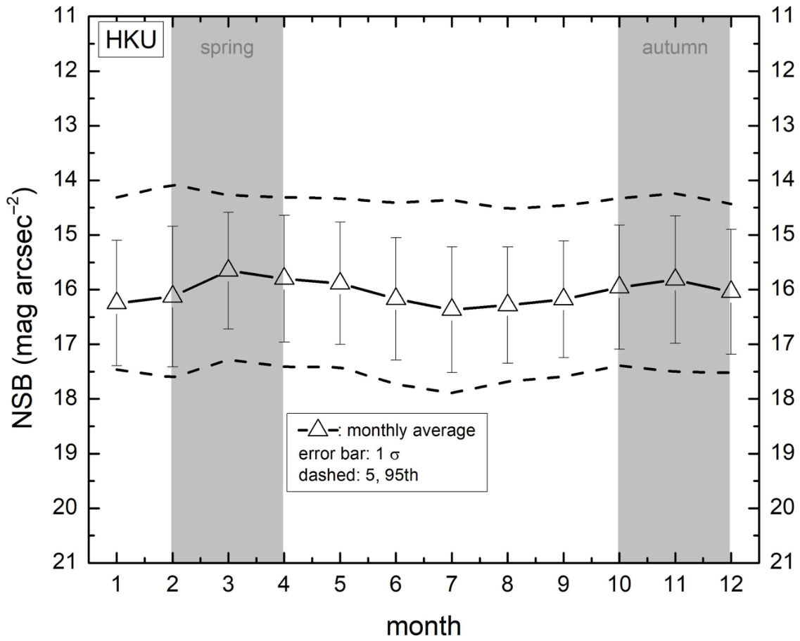
Figure 15. Same as Figure 13 for the TYPE III diverse sky condition. The straight line in the scatter plots of T s a versus NSB is the best fit weighted by errors on both variables. The figure shows run #17.
Remotesensing 18 01691 g015
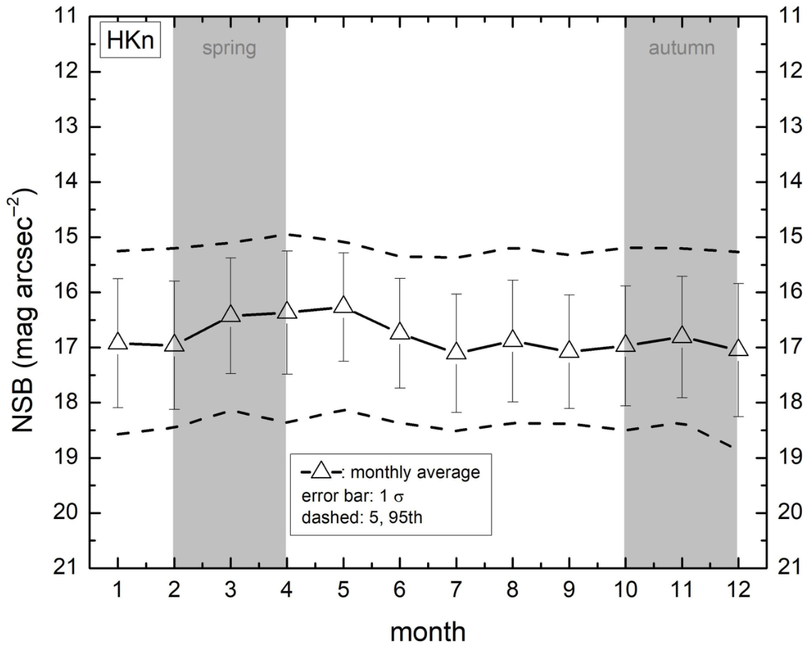
Figure 16. Typical runs ((aiaiii): #15-HKU; (bibiii): #33-iObs) with few occurrences of sudden surges in the level of T s a . They are not classified as TYPE III by definition. (ai,bi): Time-series plots on the NSB (red curves, left axis) and the cloud amount in T s a (blue curves, right axis).
Remotesensing 18 01691 g016
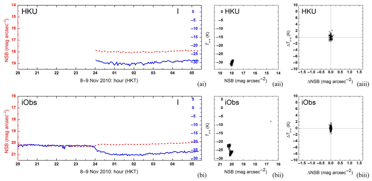
Figure 17. Typical runs ((aiaiii): #23-HKU; (bibiii): #23-iObs) with mix-TYPE properties. (ai,bi): Time-series plots on the NSB (red curves, left axis) and the cloud amount in T s a (blue curves, right axis).
Remotesensing 18 01691 g017
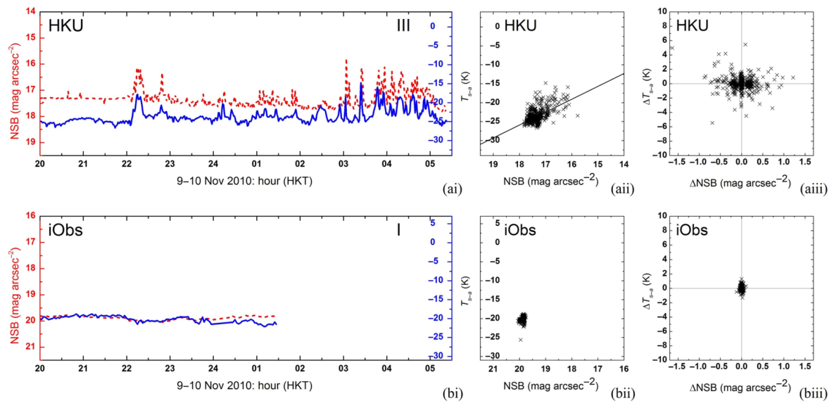
Figure 18. Typical runs ((aiaiii): #29-HKU; (bibiii): #07-iObs) with small patches of cloud rolled in and out. (ai,bi): Time-series plots on the NSB (red curves, left axis) and the cloud amount in T s a (blue curves, right axis).
Remotesensing 18 01691 g018
Figure 19. Example runs ((aiaiii): #41-HKU; (bibiii): #35-HKU) with the highest (80.0%) and lowest (42.7%) percentages of data with positive Δ T s a Δ NSB correlations, respectively. (ai,bi): Time-series plots on the NSB (red curves, left axis) and the cloud amount in T s a (blue curves, right axis).
Remotesensing 18 01691 g019
Figure 20. Scatter plot of the nightly averaged T s a and the nightly averaged NSB from all runs at the urban station HKU (squares) and the suburban station iObs (triangles).
Remotesensing 18 01691 g020
Figure 21. Scatter plot of the nightly spread of T s a and the nightly spread of NSB from all runs at the urban station HKU (squares) and the suburban station iObs (triangles).
Remotesensing 18 01691 g021
Figure 22. Scatter plot of the individual Δ T s a Δ NSB data measured at the urban station HKU. Only TYPE III data points outside the region of natural fluctuation were included. The straight line is the best fit, weighted by errors on both variables.
Remotesensing 18 01691 g022
Figure 23. Same as Figure 22 for the suburban station iObs.
Remotesensing 18 01691 g023
Table 1. Details of NSB observing locations (Abbreviations: HKI, Hong Kong Island; KLN, Kowloon; NT, New Territories; LI, Lantau Island; †, current analysis stations (total 9); BOLD, decade-long stations (6); *, cloud analysis stations (2)).
CodeFacilityLocationCoordinate (° N, ° E)Analysis Data Period
Urban locations
HKU †*The University of Hong KongPokfulam, HKI22.283, 114.140Sep 2010–Mar 2013, Dec 2014–Jun 2023
HKn †Ho Koon Nature Education cum Astronomical CentreTsuen Wan, NT22.384, 114.108Aug 2010–Mar 2013, Apr 2015–Jun 2023
TST †Hong Kong Space MuseumTsim Sha Tsui, KLN22.294, 114.171Sep 2010–Mar 2013, Jul 2017–Jun 2023
KP †King’s Park Meteorological StationKing’s Park, KLN22.312, 114.172May 2010–Mar 2013, Aug 2019–Jun 2023
FKYC †Fanling Kau Yan CollegeFanling, NT22.488, 114.138Aug 2021–Jun 2023
TPoTai Po Air Quality Monitoring StationTai Po, NT22.451, 114.165Dec 2010–Mar 2013
TSWHong Kong Wetland ParkTin Shui Wai, NT22.467, 114.009Dec 2010–Mar 2013
WTSOur Lady’s CollegeWong Tai Sin, KLN22.345, 114.197Mar 2011–Mar 2013
SShElegantia CollegeSheung Shui, NT22.493, 114.124Mar 2011–Mar 2013
STPOH Chan Kai Memorial CollegeSha Tin, NT22.366, 114.178Mar 2011–Mar 2013
Suburban locations
AP †AstroparkSai Kung, NT22.377, 114.336Nov 2010–Mar 2013, Jan 2018–Jun 2023
iObs †*Sai Kung iObservatorySai Kung, NT22.408, 114.323Sep 2010–Mar 2013, Jan 2018–Jun 2023
SH1Shui Hau ObservatoryShui Hau, LI22.222, 113.915Sep 2010–Mar 2013
Cap2 †Cape D’Aguilar Radiation Monitoring StationCape D’Aguilar, HKI22.210, 114.258May 2020–Jun 2023
Cap1Swire Institute of MarineCape D’Aguilar, HKI22.208, 114.260Nov 2010–Mar 2013
MWoSilvermine Bay CampMui Wo, LI22.274, 114.003Nov 2010–Mar 2013
TpMTap Mun Air Quality Monitoring StationSai Kung, NT22.471, 114.361Mar 2011–Mar 2013
Non-classified locations
SH2 †Shek Pik Tide Gauge StationShek Pik, LI22.220, 113.894Dec 2019–Jun 2023
TMDTuen Mun Government DepotTuen Mun, NT22.368, 113.943Nov 2010–Mar 2013
GFSGovernment Flying ServiceChek Lap Kok, LI22.296, 113.910May 2011–Mar 2013
Table 2. Total number of NSB observations conducted during the study period of 1 July 2019 to 30 June 2023.
Sample Size
Current Analysis StationSunlight-FreeSunlight- & Moonlight-Free
Urban locations
KP1,484,982432,953
TST1,432,636435,588
HKU1,515,309448,121
FKYC464,068141,559
HKn1,508,637441,958
urban6,405,6321,900,179
Suburban locations
iObs1,136,583326,775
Cap21,109,748317,292
AP1,414,018405,066
suburban3,660,3491,049,133
Non-classified location
SH21,069,635302,889
all11,135,6163,252,201
Table 3. Statistics of sunlight- and moonlight-free NSB (in mag arcsec−2) collected during the study period of 1 July 2019 to 30 June 2023.
Current Analysis StationAverage σ Times Brighter than IAU Dark Sky Standard
Urban locations
KP15.61.4251
TST15.81.4218
HKU16.51.2106
FKYC17.11.165
HKn17.51.142
urban16.41.5119
Suburban locations
iObs18.70.814
Cap219.00.711
AP19.70.86
suburban19.20.99
Non-classified location
SH218.60.916
all17.51.843
Table 4. Statistical characteristics of observed sky TYPEs.
Sky TYPERange of Nightly Averaged T s a (K)Range of Nightly σ T s a (K)
HKU
I−30.0–−13.80.5–3.0
II−3.9–−2.10.5–1.3
III−23.6–−4.91.7–7.0
iObs
I−24.9–−18.10.4–3.9
II−8.9–3.80.4–2.5
III−12.7–2.22.1–7.3
Table 5. Distributions of data points on Δ T s a Δ NSB scatter plots (see Figure 2 for the meaning of positive and negative correlations).
StationSample SizeSample Size (%) of Positively Correlated DataSample Size (%) of Negatively Correlated Data
All data
HKU10,9806968 (63.5)4012 (36.5)
iObs97476104 (62.6)3643 (37.4)
TYPE III data only
HKU61894107 (66.4)2082 (33.6)
iObs39872632 (66.0)1355 (34.0)
TYPE III data outside the ranges of natural fluctuation only (Figure 22 and Figure 23)
HKU650552 (84.9)98 (15.1)
iObs314265 (84.4)49 (15.6)
Disclaimer/Publisher’s Note: The statements, opinions and data contained in all publications are solely those of the individual author(s) and contributor(s) and not of MDPI and/or the editor(s). MDPI and/or the editor(s) disclaim responsibility for any injury to people or property resulting from any ideas, methods, instructions or products referred to in the content.