Machine Learning-Based Estimation of Terrestrial Carbon Fluxes and Analysis of Environmental Drivers Along the Eastern Coast of China

Highlights

What are the main findings?

• A systematic comparison of four machine learning models identified RF as the best approach for estimating GPP, ER, and NEP, demonstrating superior accuracy and robustness in regional carbon-flux upscaling along the eastern coast of China.
• The eastern coast of China acted as a persistent and strengthening carbon sink. Forests remained the dominant contributor, whereas wetlands, despite their high per-unit-area carbon sequestration potential, experienced a continued decline in total carbon-sink capacity due to area loss.

What are the implications of the main findings?

• The study provides an effective and scalable approach for quantifying multiple carbon-flux components, thereby improving the understanding of regional carbon dynamics in the context of environmental change.
• The results offer direct scientific support for carbon-sink management along the eastern coast of China by emphasizing the roles of forest conservation, cropland optimization, and wetland restoration in achieving carbon neutrality goals.

Abstract

The eastern coast of China, characterized by a pronounced climatic gradient and diverse ecosystems, is an ideal region for exploring the spatiotemporal dynamics of carbon fluxes and their drivers. Based on observations from eight flux tower sites, together with meteorological, remote sensing, and ecohydrological variables from 2001 to 2022, this study developed Back Propagation (BP), Support Vector Regression (SVR), Extreme Gradient Boosting (XGBoost), and Random Forest (RF) models to estimate regional gross primary productivity (GPP), ecosystem respiration (ER), and net ecosystem productivity (NEP). Among them, RF performed best, achieving validation R² values of 0.92, 0.84, and 0.83 for GPP, ER, and NEP, respectively, and was therefore selected for regional upscaling. The regional mean GPP, ER, and NEP were 1578.38, 1286.05, and 334.56 g C m⁻² yr⁻¹, respectively, indicating that the region functioned as a net carbon sink during the study period. GPP, ER, and NEP exhibited a clear spatial gradient, with higher values in the south and lower values in the north. Total regional NEP increased from 344.12 Tg C in 2001 to 517.73 Tg C in 2022, reflecting a continuous strengthening of terrestrial carbon sink strength. Forests contributed most to the regional carbon sink, while the ecosystem-level NEP contribution of croplands increased over time; by contrast, the total carbon sink of wetlands declined because of area loss. These results suggest that ecological restoration, vegetation greening, and land cover optimization jointly enhanced the carbon sink along the eastern coast of China. These findings have important implications for ecological management and green low-carbon development along the eastern coast of China.

1. Introduction

In the context of global climate change and China’s carbon peaking and carbon neutrality goals, quantifying terrestrial ecosystem carbon fluxes at the regional scale has become increasingly important [1,2,3]. The eastern coast of China, located in the East Asian monsoon region, is characterized by diverse ecosystems, intense land cover change, high population density, and concentrated socioeconomic activities, making terrestrial carbon exchange in this region highly dynamic [4,5]. Understanding the spatiotemporal variations in carbon fluxes and their driving factors is therefore essential for clarifying regional carbon cycling, safeguarding coastal ecological security, and supporting low-carbon sustainable development.

To comprehensively characterize terrestrial carbon cycling along the eastern coast of China, it is necessary to consider carbon uptake, carbon release, and their net balance. These processes are commonly quantified using gross primary productivity (GPP), ecosystem respiration (ER), and net ecosystem productivity (NEP) [6,7]. GPP reflects the capacity of ecosystems to fix atmospheric carbon dioxide, ER represents carbon release from ecosystems to the atmosphere, and NEP indicates the net carbon gain or loss of ecosystems [8]. Together, these variables capture carbon input, carbon output, and net balance, and thus serve as key indicators for understanding regional carbon cycling. An increase in regional carbon sink strength may result not only from enhanced carbon uptake, but also from changes in respiration-related carbon release. Analyzing NEP alone is therefore insufficient to fully explain the mechanisms underlying carbon sink formation. A comprehensive analysis integrating GPP, ER, and NEP is essential for disentangling the processes and drivers underlying regional carbon flux changes [9,10].

Quantifying GPP, ER, and NEP relies primarily on direct observations of ecosystem carbon exchange. Over the past few decades, the eddy covariance (EC) technique has been widely used to measure carbon fluxes between terrestrial ecosystems and the atmosphere and has become a standard approach for quantifying ecosystem carbon balance [11,12]. Building on this technique, flux observation networks such as FLUXNET, AmeriFlux, AsiaFlux, OzFlux and ChinaFLUX have been established, which together form a global EC observation system. These networks provide observations of net ecosystem exchange (NEE). Under the sign convention commonly used in flux studies, NEE is equal in magnitude but opposite in sign to NEP, and this relationship is commonly expressed as NEP = −NEE. In addition, GPP and ER can be derived from NEE using flux partitioning methods [13,14].

Although eddy covariance observations can capture carbon exchange between ecosystems and the atmosphere, their limited spatial representativeness makes them insufficient for large-scale carbon flux mapping [15]. To address this limitation, remote sensing-based methods, process-based models, and machine learning approaches have been widely used for regional carbon flux estimation. Remote sensing-based methods are effective in characterizing the spatial patterns of GPP and generating spatially explicit estimates, although uncertainties remain in arid and high-latitude regions [16]. Process-based models, such as ORCHIDEE [17], CLM [18], and LPJ [19], emphasize the mechanistic representation of carbon cycling and are advantageous for long-term scenario analysis and climate change studies. However, their performance is highly sensitive to parameter settings, initial conditions, and process representations, and substantial differences often exist among models [20].

In recent years, machine learning approaches have gained increasing attention for their ability to capture complex nonlinear relationships. By integrating flux observations with remote sensing and meteorological data, machine learning approaches provide a powerful framework for regional carbon flux upscaling [21,22]. Recent studies in China have demonstrated the potential of advanced machine learning and deep learning methods for carbon-flux upscaling in coastal ecosystems. For example, Nguyen et al. [23] integrated multi-source satellite observations with automated machine learning to predict monthly GPP, ecosystem respiration, and NEE in China’s mangrove and saltmarsh coastal wetlands. More recently, explainable sequence-based deep learning models, including LSTM and Transformer architectures, have been used to capture temporal dependencies and improve CO₂ flux prediction in China’s coastal wetlands [24]. These studies indicate that ML-based carbon-flux upscaling in China’s coastal ecosystems has increasingly moved toward automated model selection, multi-source satellite data integration, temporally explicit deep learning frameworks, and interpretable modeling. Despite these methodological advances, accurate carbon-flux estimation and interpretation still depend on a comprehensive understanding of the environmental and vegetation-related factors that regulate ecosystem carbon exchange. Previous studies have shown that ecosystem carbon fluxes are jointly regulated by meteorological, hydrological, and vegetation-related factors [22]. Xiao et al. [25] incorporated the enhanced vegetation index (EVI) and land surface water index (LSWI) as key remote sensing indices in the vegetation photosynthesis model (VPM) to estimate forest GPP. He et al. [26] emphasized the importance of vapor pressure deficit (VPD) in regulating terrestrial carbon fluxes and in evaluating ecosystem responses to future climate conditions. Moreover, climatic variables, especially air temperature and precipitation, have been widely used to estimate NEE at site, regional, and global scales because of their close links with photosynthesis and respiration [27,28]. The complex and nonlinear interactions among these variables make machine learning approaches well suited for regional carbon flux estimation and driving-mechanism analysis. Although methods such as Support Vector Regression (SVR), Artificial Neural Network (ANN), and Random Forest (RF) have been widely applied in carbon flux studies [29,30,31], most studies have focused on single indicators, especially GPP, while joint analyses of GPP, ER, and NEP remain limited. In addition, the roles of different land cover types in carbon uptake, carbon release, and net carbon balance have not been fully quantified [32]. Machine learning applications for long-term carbon-flux estimation in this region remain limited, particularly for examining land cover differences and carbon-flux responses to land cover change. These gaps hinder a more comprehensive understanding of carbon sink formation mechanisms and their implications for ecological management in coastal areas.

To address these gaps, this study focuses on the eastern coast of China. Regional carbon flux dynamics were investigated by integrating flux observations, meteorological data, remote sensing variables, and ecohydrological factors. Four machine learning models, including Back Propagation (BP), SVR, Extreme Gradient Boosting (XGBoost), and RF, were developed and compared for estimating GPP, ER, and NEP. Based on the optimal model, the spatiotemporal patterns of carbon fluxes along the eastern coast of China from 2001 to 2022 were reconstructed. Differences among major land cover types were then quantified, and the influence of land cover change on the evolution of regional carbon flux patterns was further examined. This study provides a more systematic understanding of terrestrial carbon cycling along the eastern coast of China and offers scientific support for ecological restoration, carbon sink enhancement, and sustainable land use along the eastern coast of China.

2. Data and Methods

2.1. Study Area

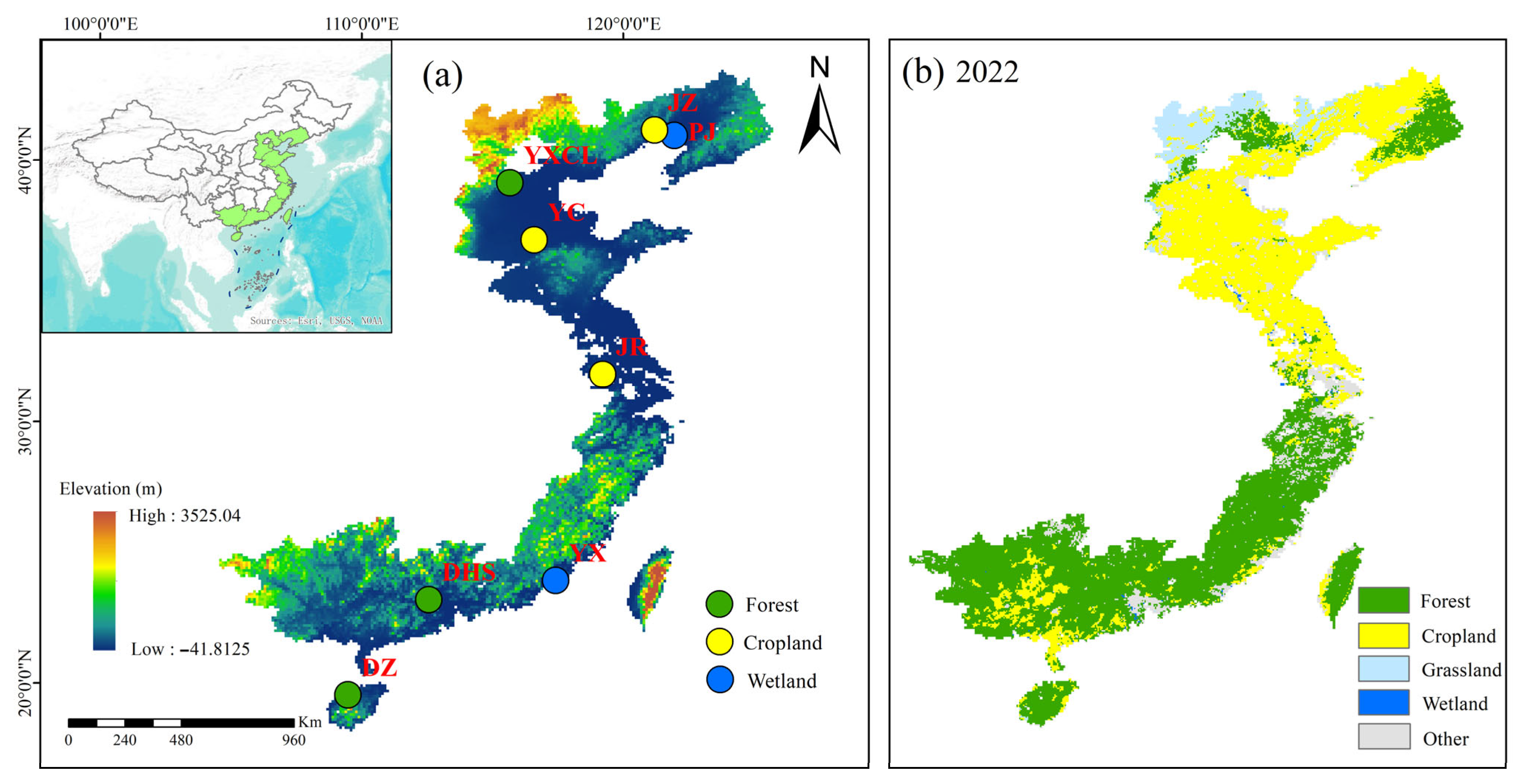
This study focuses on the eastern coastal region of China (20°09′N–43°26′N, 109°45′E–123°10′E), which ranks among the country’s most densely populated, economically developed, and rapidly urbanizing regions (Figure 1). In addition to strong human influence, the region is jointly influenced by the East Asian monsoon and land–sea thermal contrasts, with climate conditions gradually shifting from warm temperate in the north to subtropical and tropical conditions in the south. Mean annual precipitation ranges from 800 to 2000 mm and generally increases from north to south [33]. These pronounced climatic gradients have contributed to a distinct latitudinal differentiation of ecosystems across the region. The northern coastal area is characterized by warm-temperate deciduous broadleaf forests, croplands, reed wetlands, and estuarine salt marshes. The central coastal area contains extensive estuarine wetlands and broad coastal plains, whereas the southern coastal area is dominated by subtropical and tropical ecosystems, including evergreen broadleaf forests, estuarine wetlands, and mangroves [34,35]. These ecosystems differ markedly in vegetation structure, phenology, and water and carbon cycling processes, resulting in pronounced spatial heterogeneity in GPP, ER, and NEP across the region.

2.2. Dataset

2.2.1. Long-Term Carbon Flux Observations

The carbon flux data used in this study were obtained from the FLUXNET global ecosystem flux network and the ChinaFLUX terrestrial ecosystem flux network. Based on the spatial extent of the study area and the completeness of site observations, eight representative flux tower sites along the eastern coast of China were selected. The selected sites represented the major land cover types in the region, including forests, croplands, and wetlands, but there were no grassland flux tower sites in the study area (

Table 1. Basic information of flux tower sites across different land cover types.

Types	Site	Dominant Species	Location	MAT (°C)	MAP (mm)	Observation Period
CRO	JZ	Maize	121°12′6″E, 41°8′53″N	9.5	565.9	2005–2014
	YC	Wheat and Maize	116°34′13″E, 36°49′44″N	13.1	582	2003–2010
	JR	Oryza sativa L.	119°13′2″E, 31°48′24″N	15.5	1099.1	2015–2020
WET	YX	Mangrove	117°24′10″E, 23°54′23″N	21.2	1714.5	2019–2020
	PJ	Phragmites australis	121°48′27″E, 40°57′17″N	8.6	631	2018–2020
FOREST	DHS	Evergreen broadleaf	112°32′4″E, 23°10′24″N	20.9	1956	2003–2010
	YXCL	Chinese pine	115°29′29″E, 39°20′54″N	11.6	641.12	2020–2022
	DZ	Rubber plantation	109°28′30″E, 19°32′47″N	21.5–28.5	1607	2010–2018

Note: CRO, cropland; WET, wetland; FOREST, forest; MAT, mean annual temperature; MAP, mean annual precipitation.

). These sites provided long-term monthly CO₂ flux observations, yielding a total of 545 valid monthly records for model training and accuracy validation. Carbon fluxes were measured using the eddy covariance (EC) technique. The measurement systems typically consisted of a CSAT-3 three-dimensional sonic anemometer (Campbell Scientific, Logan, UT, USA) and an LI-7500 open-path infrared CO₂/H₂O gas analyzer (LI-COR, Lincoln, NE, USA), with a sampling frequency of 10 Hz [10]. Raw site data were processed according to ChinaFLUX quality control protocols, including outlier removal, coordinate rotation, time-lag correction, WPL density correction, spectral loss correction, gap filling, and flux partitioning [36,37]. These flux tower observations provided essential ground-based constraints for regional carbon flux estimation and served as training and validation data for the machine learning models. Their long-term records also captured seasonal and interannual variations in carbon uptake and release across different ecosystems, thereby improving the reliability of regional-scale estimates.

2.2.2. Remote Sensing and Meteorological Data

The land environment is inherently complex and dynamic. To accurately estimate regional carbon fluxes, this study utilizes a multi-source environmental dataset covering the period from 2001 to 2022, including remote sensing, meteorological, and topographic data. All data were standardized to a monthly scale and resampled to a 0.1° × 0.1° spatial resolution to ensure consistency.

The vegetation index was derived from the MODIS MOD09A1 surface reflectance product, with an original spatial resolution of 500 m and a time range from February 2000 to the present. Based on the MOD09A1 reflectance data, the Enhanced Vegetation Index (EVI) and the Land Surface Water Index (LSWI) were calculated to represent vegetation growth status and canopy-soil moisture information, respectively. The formulas for EVI and LSWI are as follows:

$$\mathit{EVI} = 2.5 \times {\displaystyle \frac{{\rho }_{\mathit{NIR}} - {\rho }_{\mathit{Red}}}{{\rho }_{\mathit{NIR}} + 6{\rho }_{\mathit{Red}} - 7.5{\rho }_{\mathit{Blue}} + 1}}$$

(1)

where ${\rho }_{NIR}$, ${\rho }_{Red}$ and ${\rho }_{Blue}$ represent the reflectances in the near-infrared, red, and blue bands, respectively.

$$\mathit{LSWI} = {\displaystyle \frac{{\rho }_{\mathit{NIR}} - {\rho }_{\mathit{SWIR}}}{{\rho }_{\mathit{NIR}} + {\rho }_{\mathit{SWIR}}}}$$

(2)

where ${\rho }_{NIR}$ and ${\rho }_{SWIR}$ represent the reflectances in the near-infrared and shortwave infrared bands, respectively.

Meteorological variables were obtained from the ERA5-Land reanalysis dataset, with a spatial resolution of 0.1° and temporal coverage from 1950 to the present [38]. For regional carbon flux estimation, 2 m air temperature (T2M), 2 m dew point temperature (D2M), surface downward shortwave radiation (SSRD), high vegetation leaf area index (LAI_H), and vegetation transpiration (EVAVT) were extracted. Vapor pressure deficit (VPD), which represents atmospheric water demand, was calculated from T2M and D2M follows Allen et al. [39]:

$$VPD = 0.6108 \left[ \mathit{exp}\left( {\displaystyle \frac{17.27T_{2M}}{T_{2M}+237.3}} \right) - \mathit{exp}\left( {\displaystyle \frac{17.27D_{2M}}{D_{2M}+237.3}} \right) \right]$$

(3)

To better represent the hydrological and photosynthetic controls on regional carbon fluxes, two additional datasets were used in this study. Monthly precipitation (PPT) data from the China Meteorological Forcing Dataset (CMFD) were used to characterize water input and moisture availability [40]. Solar-induced chlorophyll fluorescence (SIF) data from the Chinese Ecosystem Research Network (CERN) were used as a direct proxy for vegetation photosynthetic activity [41]. Detailed information on these datasets is provided in

Table 2. Summary of datasets used in this study.

Research Data	Variables	Data Source URL
ChinaFLUX	Ecosystem carbon fluxes	https://chinaflux.org/ (accessed on 11 May 2026)
MODIS	Enhanced vegetation index (EVI)	https://www.earthdata.nasa.gov/ (accessed on 11 May 2026)
	Land surface water index (LSWI)
	MODIS Land Cover Type Product
ERA5-Land	2 m temperature (T2M)	https://cds.climate.copernicus.eu/ (accessed on 11 May 2026)
	2 m dewpoint temperature (D2M)
	Evaporation from vegetation transpiration (EVAVT)
	Surface solar radiation downwards (SSRD)
	Leaf area index high vegetation (LAI_H)
	Vapor pressure deficit (VPD)
CMFD	Precipitation (PPT)	https://data.tpdc.ac.cn/ (accessed on 11 May 2026)
CERN	Solar-induced chlorophyll fluorescence (SIF)	https://nesdc.org.cn/ (accessed on 11 May 2026)

.

2.2.3. Land Cover and Global Carbon Flux Products

Land cover data were derived from the MODIS MCD12C1 product with a spatial resolution of 0.05°. This product provides continuous temporal coverage and a standardized land cover classification system, and has been widely used in regional and global studies. In this study, the IGBP classification scheme was used, and the original land cover classes were reclassified into five broader categories: forest, grassland, cropland, wetland, and other types. Forest included evergreen needleleaf forest, evergreen broadleaf forest, deciduous needleleaf forest, deciduous broadleaf forest, and mixed forest. Cropland included croplands and cropland/natural vegetation mosaics. Grassland corresponded to the IGBP grassland class, and wetland corresponded to the permanent wetland class. Other types included the remaining land-cover classes not included in the above four categories.

The FLUXCOM project integrates remote sensing observations, ground-based flux measurements, and machine learning methods, and has been widely used in global carbon cycle research [42,43]. In this study, the FLUXCOM-X-BASE carbon flux product was used. This dataset provides global gridded estimates of carbon fluxes from 2001 to 2021 by upscaling eddy covariance observations with machine learning. It has a spatial resolution of 0.05° and was aggregated to a monthly scale for this study. Because FLUXCOM-X-BASE provides net ecosystem exchange (NEE), NEP was calculated as the negative of NEE. Ecosystem respiration (ER) was derived from GPP and NEP as ER = GPP − NEP. To ensure consistency with other datasets, the product was resampled to 0.1° (Table 2).

2.3. Methods

2.3.1. Machine Learning Models

BP neural network is a multilayer feed-forward neural network trained using the backpropagation approach. It can learn and approximate complex nonlinear relationships between inputs and outputs. Its basic structure includes an input layer, one or more hidden layers, and an output layer. During training, it can continuously adjust the connection weights and thresholds between layers to ensure optimal output results [44].

Support Vector Regression (SVR) is a supervised learning approach derived from statistical learning theory. It is particularly effective for nonlinear regression problems in small-sample settings [45]. By means of a kernel function, SVR projects input variables into a high-dimensional feature space, where nonlinear patterns can be modeled while model complexity is kept under control according to the principle of structural risk minimization. These characteristics make SVR well suited for ecological and environmental studies, and it has therefore been increasingly used in such fields in recent years [46,47].

Random Forest (RF) is an ensemble learning approach based on the Bagging strategy. It achieves stable predictive performance by constructing multiple decision trees and combining their outputs [48]. During model development, RF randomly samples both observations and features, which increases diversity among trees and helps reduce overfitting. In addition, RF performs well on high-dimensional data, shows strong resistance to noise, and is able to capture the complex nonlinear patterns often present in ecological systems. These characteristics make RF well suited for studies of global water and carbon fluxes [42,43].

XGBoost, proposed by Chen and Guestrin [49] in 2016, is an efficient ensemble approach built on gradient boosted trees and can be regarded as an enhanced version of the traditional GBRT method [49]. It introduces a regularization term into the objective function to constrain model complexity and lower the risk of overfitting [50]. Meanwhile, XGBoost improves computational efficiency through parallel processing without sacrificing predictive accuracy. It is suitable for classification, regression, and ranking tasks, and its ability to handle missing values makes it effective for high-dimensional and noisy datasets [51].

2.3.2. SHAP-Based Feature Importance Analysis

The Shapley Additive Explanations (SHAP) method is used to assess the contribution of each input feature to model predictions. Based on the Shapley value framework from cooperative game theory, SHAP calculates the marginal contribution of each feature under different combinations of features, thereby revealing the prediction mechanism of complex models [52,53]. This method not only uses the average prediction value of the training data as a baseline, but also quantifies the direction (positive or negative) and magnitude of each feature’s contribution to individual sample predictions. Compared to traditional feature importance metrics, SHAP provides both global and local explanations, offering a more comprehensive understanding of the relative influence of input variables and their potential interactions within the model.

2.3.3. Mann–Kendall Test and Sen’s Slope Estimator

The Mann–Kendall test is a non-parametric method widely used to detect monotonic trends in time-series data. Because it does not require the data to follow a normal distribution, it is suitable for ecological and climatic time series that may contain non-normality or outliers.

For a time series $x_1,x_2,\dots ,x_n$, the Mann–Kendall statistic $S$ is calculated as

$$S=\sum _{i=1}^{n-1}{\displaystyle \sum _{j=i+1}^n}sgn\left(x_j-x_i\right)$$

(4)

where

$$sgn\left(x_j-x_i\right)=\{\begin{array}{c} 1, x_j-x_i>0\\ 0, x_j-x_i=0\\ -1, x_j-x_i<0\end{array}$$

(5)

A positive $S$ value indicates an increasing trend, whereas a negative $S$ value indicates a decreasing trend. The statistical significance of the trend was evaluated using the standardized test statistic $Z$, and trends were considered statistically significant at $p<0.05$. Sen’s slope estimator was used to quantify the magnitude of the trend. It is calculated as the median of all pairwise slopes between data points:

$$\beta =\mathrm{m}\mathrm{e}\mathrm{d}\mathrm{i}\mathrm{a}\mathrm{n}({\displaystyle \frac{x_j-x_i}{t_j-t_i}}), j>i$$

(6)

where $x_i$ and $x_j$ are the carbon flux values corresponding to years $t_i$ and $t_j$, respectively, and $\beta$ represents the rate of change per unit time. A positive Sen’s slope indicates an increasing trend, whereas a negative value indicates a decreasing trend.

2.4. Data Processing and Statistical Analysis

Nine environmental variables derived from meteorological, remote sensing, and ecohydrological data were selected as predictors for machine learning-based estimation of carbon fluxes. Given the limited number of available flux sites within each ecosystem type, ecosystem-specific machine learning models were not constructed; instead, a unified regional model was adopted for regional upscaling. The flux dataset was randomly divided into training and testing sets, with 80% of the observations (436 site-months) used for training and the remaining 20% (109 site-months) used for testing. The trained models were then applied to the testing set to evaluate the predictive performance of the four machine learning approaches. Instead, a unified regional model was adopted for regional upscaling. Model performance under different feature combinations was assessed using three standard metrics: the coefficient of determination (R²), root mean square error (RMSE), and mean absolute error (MAE). R² reflects the explanatory power of the model, while RMSE and MAE quantify prediction errors between observed and estimated values. The formulas for these metrics are given below:

$$R^2={\displaystyle \frac{{\left({\sum }_{i=1}^n\left(Q_i^m-\overline{Q}\right)\left(Q_i^o-\overline{Q}\right)\right)}^2}{\left({\sum }_{i=1}^n{\left(Q_i^m-\overline{Q}\right)}^2\right)\left({\sum }_{i=1}^n{\left(Q_i^o-\overline{Q}\right)}^2\right)}}$$

(7)

$$RMSE=\sqrt{{\displaystyle \frac{{\sum }_{i=1}^n{\left(Q_i^o-Q_i^m\right)}^2}{n}}}$$

(8)

$$MAE={\displaystyle \frac{{\sum }_{i=1}^n\left|Q_i^o-Q_i^m\right|}{n}}$$

(9)

where ${\mathrm{Q}}_{\mathrm{i}}^{\mathrm{o}}$ and ${\mathrm{Q}}_{\mathrm{i}}^{\mathrm{m}}$ denote the observed and modeled values of carbon flux, respectively; $\stackrel{\mathrm{ˉ}}{\mathrm{Q}}$ is the mean value of the corresponding variable; $\mathrm{n}$ is the number of samples; and $\mathrm{i}$ is the sample index.

3. Results

3.1. Input Variable Continuity and Feature-Space Consistency

Given the limited temporal coverage of flux tower observations, we assessed the reliability of early-period estimation for 2001–2005 by examining the continuity of input variables and their consistency with the training feature space. Because the RF model estimates carbon fluxes from environmental predictors, it is important to determine whether the predictor conditions in the early 2000s were comparable to those represented by the training samples. As shown in Figure S1, the nine input variables, including T2M, EVI, VPD, LSWI, EVAVT, LAI_H, SSRD, PPT, and SIF, generally showed continuous interannual variations during 2001–2022, without obvious structural breaks. Vegetation-related variables such as EVI and SIF, together with LSWI, showed consistent temporal changes, reflecting long-term variations in vegetation activity and surface moisture conditions. LAI_H showed very weak interannual variation, which is reasonable because it is derived from ERA5-Land and mainly represents background high-vegetation structure and spatial differences, while interannual vegetation dynamics were primarily captured by EVI, LSWI, and SIF. Climatic and surface-energy variables, including T2M, VPD, PPT, EVAVT, and SSRD, also showed continuous year-to-year fluctuations.

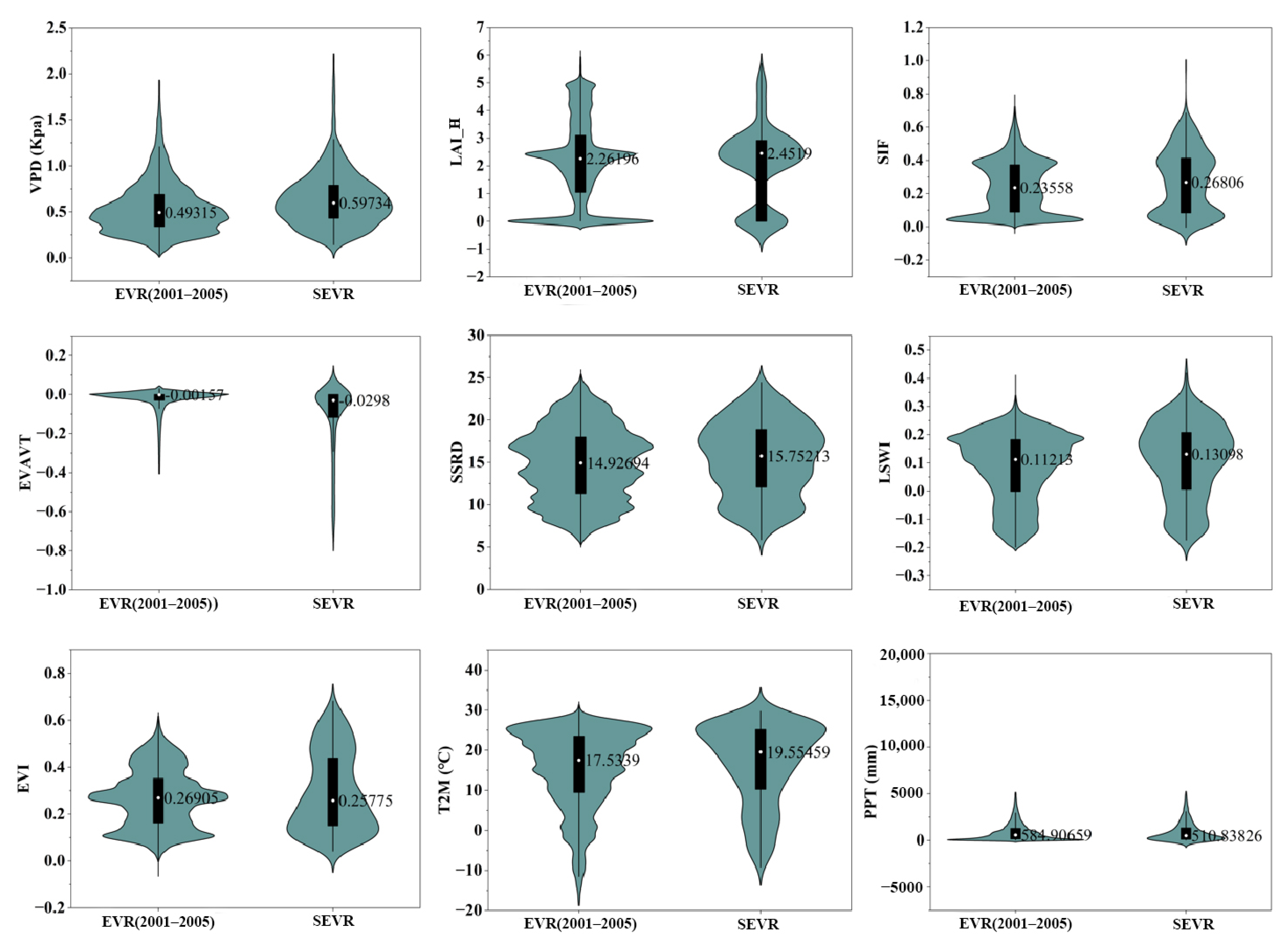
To further evaluate early-period hindcasting, we compared the distributions of the nine input variables between 2001 and 2005 and the flux-tower training period (Figure 2). The results showed that the early-period distributions largely overlapped with those of the training period for most predictors, suggesting that the environmental conditions during 2001–2005 generally remained within the feature space covered by the training samples. These results indicate that the early-period carbon flux estimates were not generated under substantially different input conditions and provide additional support for the reliability of regional carbon flux hindcasting.

3.2. Model Performance Comparison and Validation

3.2.1. Overall Model Performance and Optimal Model Selection

The optimized hyperparameter settings for each model are shown in

Table 3. Control parameters of the machine learning model.

Model	Parameter	Specification and Range
BP	Learning rate	0.01
	Iterations number	1000
	Number of hidden neurons	[6]
	Error threshold	1 × 10−6
RF	n_trees	500
	min_leaf_size	4
SVR	C	4
	kernel scale	1
	Epsilon	0.05
XGBoost	Learning rate	0.1
	number of iterations	100
	max_depth	3
	subsample	0.9
	colsample_bytree	1

. Given the limited sample size (545 samples), the final parameter combinations were selected based on validation and cross-validation performance in terms of R², RMSE, and MAE. The chosen settings helped improve predictive accuracy while limiting overfitting across models.

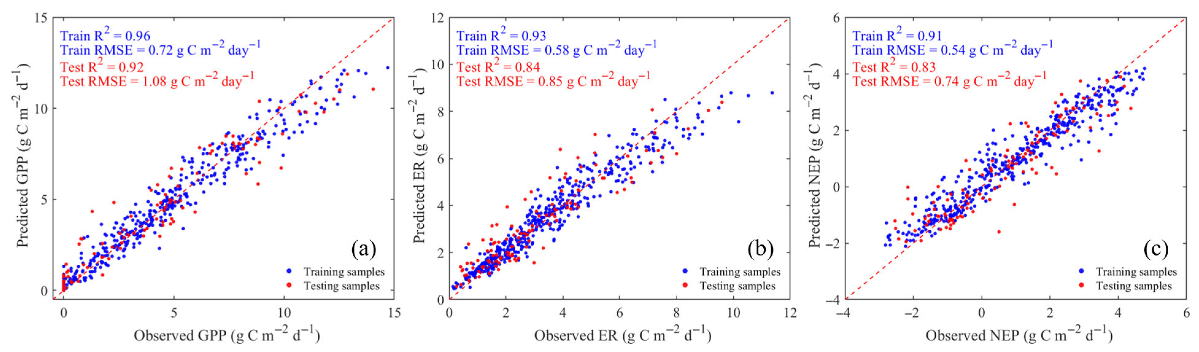
To compare model performance, RF, XGBoost, SVR, and BP were evaluated using both the validation results under the optimal parameter settings and the results of ten-fold cross-validation (

Table 4. Performance comparison of different models on the training and validation sets.

Variable	Approach	R2		RMSE		MAE
		T	V	T	V	T	V
GPP	BP	0.89	0.88	1.13	1.28	0.79	0.86
	SVR	0.91	0.91	1.00	1.06	0.74	0.77
	XGBoost	0.96	0.91	0.73	1.07	0.54	0.78
	RF	0.96	0.92	0.72	1.07	0.51	0.78
ER	BP	0.83	0.81	0.83	0.83	0.63	0.65
	SVR	0.86	0.84	0.72	0.77	0.54	0.59
	XGBoost	0.93	0.85	0.59	0.85	0.45	0.67
	RF	0.93	0.84	0.58	0.85	0.43	0.65
NEP	BP	0.79	0.74	0.97	1.10	0.74	0.82
	SVR	0.81	0.81	0.87	0.96	0.63	0.73
	XGBoost	0.89	0.80	0.61	0.86	0.46	0.68
	RF	0.91	0.83	0.54	0.74	0.40	0.57

Note: T and V denote the performance on the training and validation sets, respectively. RMSE and MAE are expressed in g C m⁻² d⁻¹.

and

Table 5. Performance comparison of different models under 10-fold cross-validation.

Variable	Approach	R2		RMSE		MAE
		MT	MV	MT	MV	MT	MV
GPP	BP	0.90	0.85	1.14	1.31	0.82	0.98
	SVR	0.92	0.87	0.98	1.22	0.71	0.89
	XGBoost	0.96	0.87	0.72	1.24	0.52	0.91
	RF	0.96	0.89	0.70	1.14	0.50	0.82
ER	BP	0.83	0.77	0.79	0.88	0.60	0.67
	SVR	0.87	0.79	0.69	0.87	0.52	0.66
	XGBoost	0.92	0.80	0.60	0.85	0.41	0.65
	RF	0.93	0.80	0.54	0.83	0.39	0.63
NEP	BP	0.76	0.69	1.03	1.06	0.78	0.89
	SVR	0.84	0.73	0.84	1.05	0.62	0.78
	XGBoost	0.88	0.73	0.64	0.99	0.48	0.76
	RF	0.92	0.77	0.59	0.90	0.44	0.67

Note: MT and MV denote the mean training and validation performance across the 10 folds, respectively. RMSE and MAE are expressed in g C m⁻² d⁻¹.

). For GPP estimation, the RF model achieved a validation R² of 0.92, which was higher than those of XGBoost and SVR (both 0.91). In the ten-fold cross-validation, the RF model yielded an R² of 0.89, with an RMSE of 1.14 and an MAE of 0.82. These results indicated that the RF model had good predictive accuracy and stability for GPP estimation. For ER estimation, the differences among models were relatively small. Although XGBoost achieved a slightly higher validation R² than RF under the optimal parameter settings, RF showed lower error values and more favorable performance in 10-fold cross-validation. This indicates that RF was more balanced and stable overall for ER estimation. For NEP estimation, the RF model achieved the highest validation R² of 0.83, indicating a stronger ability to capture the variation in net carbon flux. It also showed relatively favorable RMSE and MAE values in the 10-fold cross-validation, indicating that RF delivered more accurate and balanced performance for NEP estimation compared to the other three models (Figure 3). Overall, all four models were capable of reproducing regional carbon flux variability to some extent. Among them, RF showed the most favorable overall performance.

3.2.2. Leave-One-Site-Out Cross-Validation

Although the RF model performed well in 10-fold cross-validation, random partitioning may provide an overly optimistic estimate of model performance. This concern is particularly relevant because the study area spans strong environmental gradients and the number of available flux sites is limited. We therefore used leave-one-site-out cross-validation (LOSO-CV) as a stricter test, excluding one site from model training and using it exclusively for testing in each iteration. The LOSO-CV results showed clear differences among sites (

Table 6. Performance of GPP, ER, and NEP by flux site in leave-one-site-out cross-validation.

Type	Site	GPP			ER			NEP
		R2	RMSE	MAE	R2	RMSE	MAE	R2	RMSE	MAE
CRO	JZ	0.89	1.32	1.11	0.71	1.16	0.87	0.73	1.05	0.83
	YC	0.80	2.06	1.67	0.78	1.40	1.08	0.59	1.40	1.06
	JR	0.61	2.07	1.65	0.61	1.17	0.85	0.30	1.53	1.29
WET	YX	0.18	2.73	1.98	0.13	1.45	1.38	0.23	0.72	0.55
	PJ	0.87	1.20	0.81	0.73	1.09	0.82	0.55	1.08	0.78
FOREST	DHS	0.73	0.96	0.66	0.69	1.11	0.97	0.72	0.87	0.72
	YXCL	0.76	1.89	1.56	0.80	1.10	0.97	0.70	1.33	1.01
	DZ	0.53	1.95	1.66	0.33	1.60	1.28	0.28	1.31	1.05
	Median	0.75	1.92	1.61	0.70	1.17	0.97	0.57	1.20	0.92

Note: RMSE and MAE are expressed in g C m⁻² d⁻¹.

). In general, GPP and ER were predicted with moderate to high accuracy at most sites, whereas NEP was less well predicted and showed larger variability among sites. The median R² values were 0.75 for GPP, 0.70 for ER, and 0.57 for NEP. JZ, PJ, and DHS performed relatively well, whereas YX showed lower predictive accuracy. The site-level results further indicated that model accuracy differed not only among ecosystem types, but also among sites within the same ecosystem type, suggesting that local environmental heterogeneity remained an important source of uncertainty. Consistent with this stricter validation design, LOSO-CV performance was lower than that of random 10-fold cross-validation, indicating that prediction became more difficult when the model was applied to unseen sites. Nevertheless, the RF model still showed reasonable agreement with the observations for GPP and ER at most sites.

3.3. Distinct Environmental Controls on GPP, ER, and NEP Revealed by SHAP Analysis

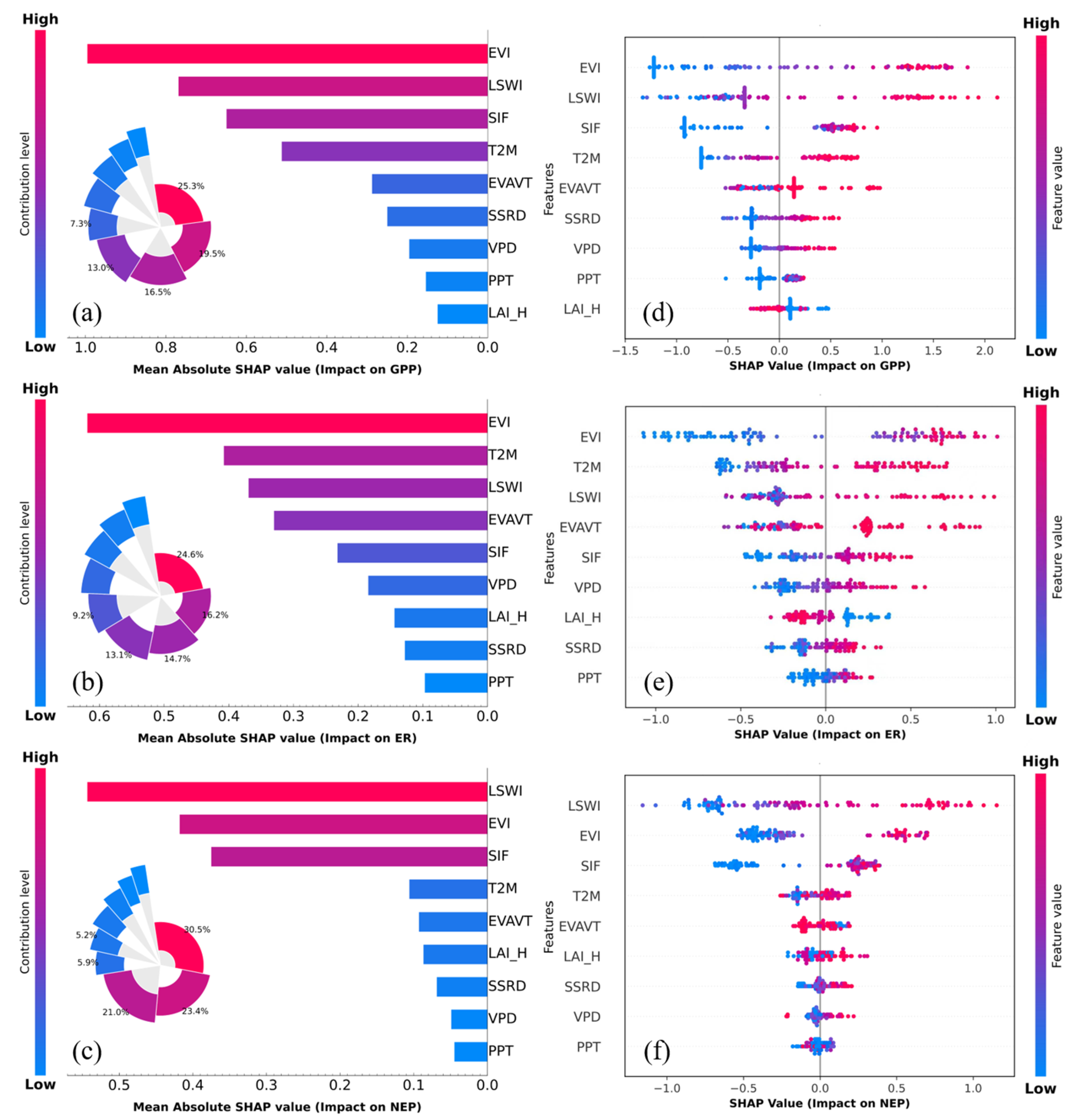
Figure 4 presents the SHAP importance rankings and summary plots for the RF model, showing the relative contribution of each predictor and the direction of its effect on the target variables. For GPP and NEP, high values of EVI, LSWI, and SIF were generally associated with positive SHAP values. For ER, higher EVI and T2M values were more often associated with positive SHAP values, indicating positive contributions of vegetation activity and temperature to ER predictions. In contrast, PPT, VPD, LAI_H, and SSRD showed relatively weak contributions across the three carbon-flux components. The results indicate that vegetation-related, water-related, and climatic variables jointly contributed to the spatial variation in GPP, ER, and NEP. Among the three carbon-flux components, GPP was more closely associated with vegetation condition and photosynthetic activity, ER reflected the combined influence of temperature, vegetation activity, and moisture conditions, and NEP was more strongly linked to water status.

3.4. SHAP-Informed All-Variable Input Perturbation Analysis

The previous ten-fold cross-validation mainly assessed the predictive performance of the RF model under different sample partitioning schemes. However, in practical regional applications, carbon-flux estimates may also be affected by uncertainties in the environmental predictor datasets. Therefore, in addition to conventional model validation, we further evaluated the robustness of the trained RF model to input perturbations. Unlike the original climate-only perturbation experiment, the revised analysis was extended to all nine input variables, including T2M, EVI, VPD, LSWI, EVAVT, LAI_H, SSRD, PPT, and SIF. The perturbation magnitudes were defined according to the physical meaning and observed range of each variable. Specifically, additive perturbations were applied to T2M, EVI, and LSWI, while relative perturbations were applied to VPD, LAI_H, SSRD, PPT, and SIF. Because EVAVT follows a flux sign convention and is mainly represented by negative values, the perturbation was applied to the magnitude of EVAVT, rather than to its numerical sign. During the perturbation experiment, the model structure and hyperparameters were kept fixed, and only one input variable was perturbed at a time.

As shown in

Table 7. Summary of prediction robustness for GPP, ER, and NEP under input perturbation scenarios.

Variable	Scenario	GPP			ER			NEP
		R2	RMSE	MAE	R2	RMSE	MAE	R2	RMSE	MAE
Baseline	-	0.918	1.075	0.783	0.838	0.853	0.646	0.831	0.720	0.534
EVI	+0.05	0.899	1.195	0.924	0.815	0.891	0.700	0.805	0.774	0.580
	−0.05	0.905	1.155	0.819	0.814	0.894	0.689	0.810	0.764	0.570
LSWI	+0.05	0.891	1.241	0.899	0.813	0.895	0.688	0.763	0.854	0.599
	−0.05	0.883	1.286	0.871	0.809	0.904	0.686	0.768	0.844	0.622
T2M	+3 °C	0.912	1.117	0.831	0.803	0.919	0.696	0.828	0.726	0.543
	−3 °C	0.910	1.128	0.785	0.823	0.870	0.659	0.817	0.750	0.547
SIF	+20%	0.912	1.115	0.821	0.828	0.859	0.649	0.828	0.726	0.540
	−20%	0.915	1.093	0.788	0.829	0.856	0.652	0.808	0.769	0.571
|EVAVT|	+20%	0.922	1.052	0.770	0.834	0.844	0.637	0.831	0.721	0.535
	−20%	0.915	1.097	0.801	0.819	0.881	0.659	0.827	0.728	0.544
VPD	+20%	0.915	1.098	0.799	0.831	0.851	0.641	0.830	0.722	0.534
	−20%	0.917	1.085	0.783	0.825	0.865	0.653	0.831	0.720	0.539
LAI_H	+20%	0.910	1.128	0.824	0.818	0.883	0.673	0.810	0.761	0.570
	−20%	0.916	1.088	0.797	0.821	0.875	0.672	0.817	0.749	0.576
SSRD	+20%	0.918	1.076	0.784	0.826	0.863	0.661	0.823	0.718	0.552
	−20%	0.903	1.173	0.828	0.817	0.885	0.665	0.821	0.737	0.550
PPT	+20%	0.920	1.078	0.782	0.829	0.856	0.649	0.834	0.714	0.532
	−20%	0.918	1.076	0.784	0.831	0.851	0.646	0.832	0.718	0.534

Note: RMSE and MAE are expressed in g C m⁻² d⁻¹.

, the RF predictions remained generally stable under all single-variable perturbation scenarios. For GPP, the baseline R², RMSE, and MAE were 0.918, 1.075, and 0.783, respectively. Under input perturbations, R² ranged from 0.883 to 0.922, RMSE ranged from 1.052 to 1.286, and MAE ranged from 0.770 to 0.924. The largest changes in GPP performance were mainly associated with LSWI and EVI perturbations. For ER, the baseline R², RMSE, and MAE were 0.838, 0.853, and 0.646, respectively. Under perturbation scenarios, R² remained between 0.803 and 0.834, RMSE ranged from 0.844 to 0.919, and MAE ranged from 0.637 to 0.700, with T2M and EVI perturbations causing relatively larger changes. For NEP, the baseline R², RMSE, and MAE were 0.831, 0.720, and 0.534, respectively. Under perturbations, R² ranged from 0.763 to 0.834, RMSE ranged from 0.714 to 0.854, and MAE ranged from 0.532 to 0.623. NEP was most sensitive to LSWI perturbation, indicating that uncertainty in surface moisture-related information may have a relatively stronger influence on net carbon balance estimation.

Overall, although the magnitude of model response differed among variables and flux components, no single-variable perturbation led to a substantial deterioration in model performance. The variables that induced relatively larger changes, such as LSWI and EVI for GPP and NEP and T2M for ER, were generally consistent with the SHAP-based interpretation of key environmental controls. These results suggest that the RF-based estimates were reasonably robust to plausible input uncertainties, while also confirming that uncertainties in key vegetation- and moisture-related predictors should be carefully considered in regional carbon-flux upscaling.

3.5. Spatiotemporal Patterns of Carbon Fluxes

3.5.1. Spatial Patterns of Carbon Fluxes Along the Eastern Coast of China

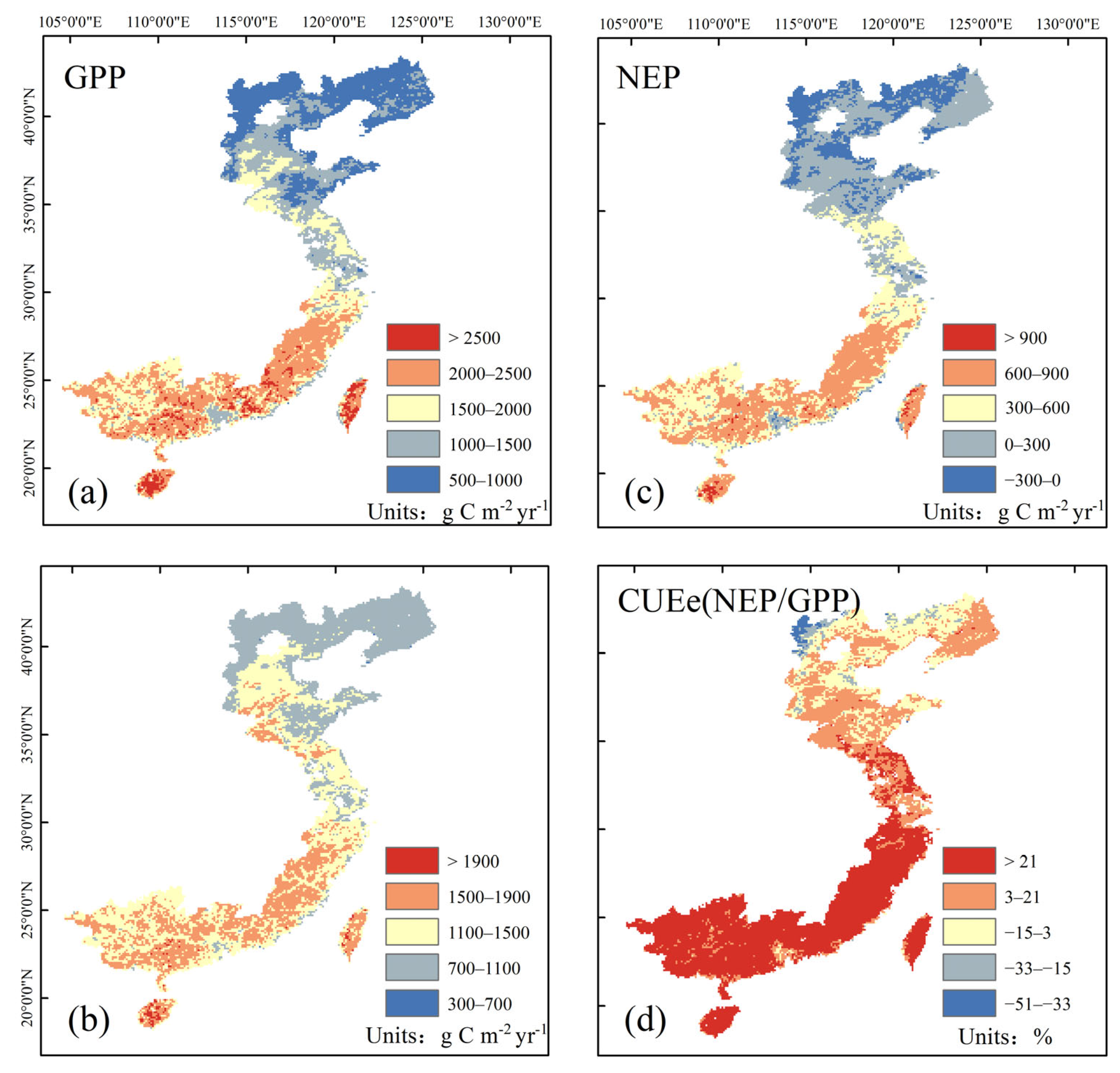
As shown in Figure 5, carbon fluxes and carbon use efficiency (CUE) along the eastern coast of China exhibited pronounced spatial heterogeneity during 2001–2022. Over the study period, the regional mean GPP, ER, and NEP were 1578.38, 1286.05, and 334.56 g C m⁻² yr⁻¹, respectively, while the mean CUE was 0.21, indicating an overall net carbon sink. Spatially, GPP, ER, and NEP all decreased from south to north. High values were mainly concentrated in the South China coastal region, Hainan Island, and Taiwan Island, whereas low values were primarily distributed along the northern and northeastern coast of China. GPP was generally high in southern China and exceeded 2000 g C m⁻² yr⁻¹ in some areas. ER showed a spatial pattern broadly similar to that of GPP, with high values likewise occurring in the southeastern coastal region and Hainan Island. NEP also displayed a clear latitudinal gradient, with relatively high values in Guangdong, Fujian, and Hainan, while most northern coastal areas were characterized by medium to low values, and some local areas approached zero or even became negative. CUE was relatively high in the southeastern coastal region and Hainan Island but lower in the northern coastal region, and its high-value areas largely coincided with those of NEP. Overall, carbon fluxes and CUE along the eastern coast of China showed a distinct south-to-north spatial gradient during the study period.

3.5.2. Interannual Variations in Carbon Fluxes Along the Eastern Coast of China

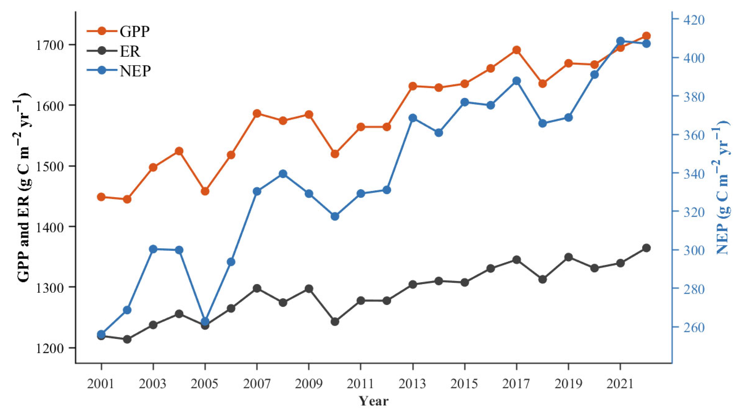
From 2001 to 2022, GPP, ER, and NEP in the eastern coastal region of China showed overall increasing trends with interannual fluctuations (Figure 6). During this period, GPP increased from 1448.76 to 1714.32 g C m⁻² yr⁻¹, an increase of 18.33%; ER increased from 1219.44 to 1364.57 g C m⁻² yr⁻¹, an increase of 11.90%; and NEP increased from 256.09 to 407.22 g C m⁻² yr⁻¹, an increase of 59.01%. Based on the values in 2001 and 2022, the average annual increases in GPP, ER, and NEP were estimated at 12.65, 6.91, and 7.20 g C m⁻² yr⁻¹, respectively. Overall, GPP and ER exhibited similar temporal patterns, but the cumulative increase in GPP was greater than that in ER, corresponding to the overall increase in NEP. This result indicates an enhanced net carbon uptake in the regional ecosystem during the study period.

4. Discussion

4.1. Comparison of Carbon Fluxes Between RF Estimates and FLUXCOM-X-BASE

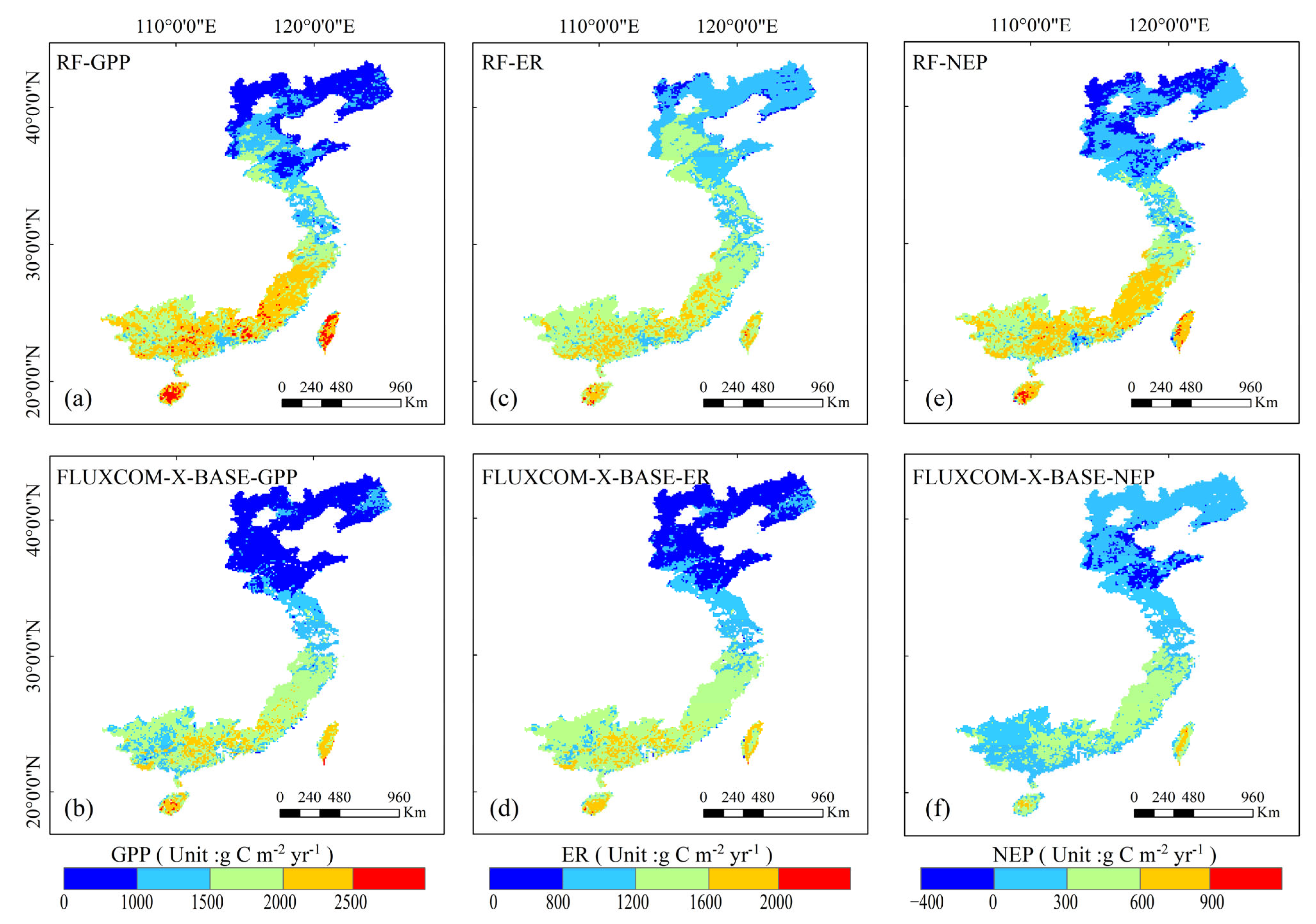
During the overlapping period from 2001 to 2021, the RF-based estimates were compared with FLUXCOM-X-BASE over eastern coastal China. FLUXCOM-X-BASE was used as the main benchmark because of its updated framework and longer temporal coverage [54]. In terms of spatial patterns, the RF estimates and FLUXCOM-X-BASE showed broadly consistent distributions across the study region. Both datasets captured a clear north–south gradient in carbon fluxes, with lower values in the northern part of eastern coastal China and higher values in the southern part. The locations of high- and low-value regions were also generally consistent between the two datasets (Figure 7), indicating that the RF-based predictions reasonably represented the main spatial distribution of regional carbon fluxes.

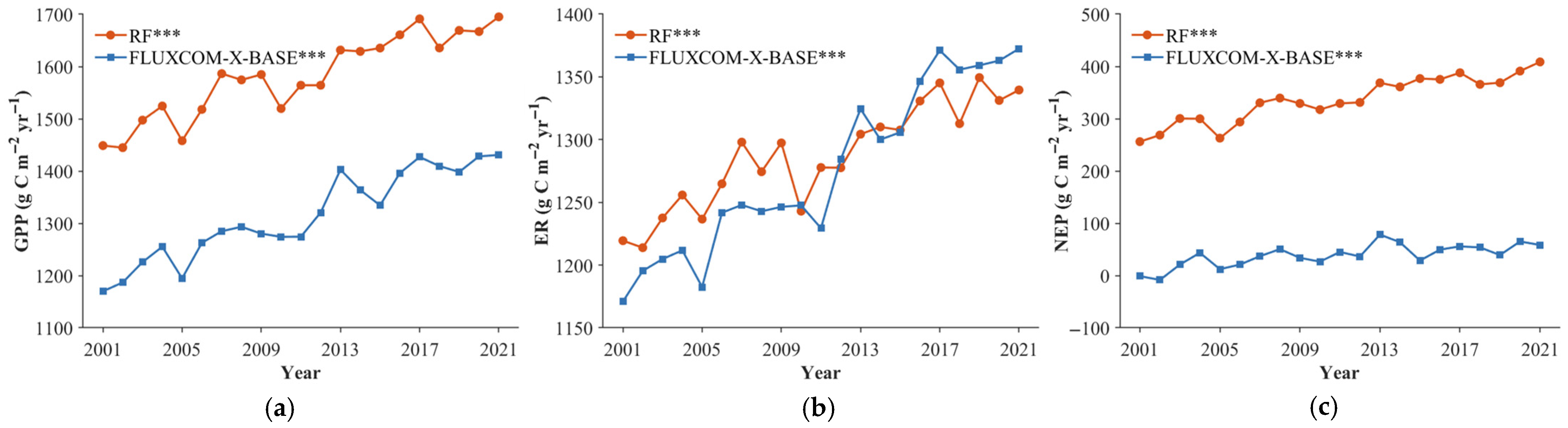
Regarding interannual variation, both the RF estimates and FLUXCOM-X-BASE showed increasing trends in GPP, ER, and NEP during 2001–2021 (Figure 8). This consistency suggests that the long-term enhancement of regional carbon uptake was captured by both datasets, providing additional support for the increasing carbon sink trend identified in this study. However, differences remained in the amplitude of interannual variability, especially for NEP. Compared with FLUXCOM-X-BASE, the RF estimates showed stronger interannual fluctuations. This difference may reflect the different objectives and scaling strategies of the two approaches. FLUXCOM-X-BASE is a global upscaling product designed to provide spatially consistent estimates across diverse climates and ecosystem types, whereas the RF model in this study was trained using flux tower observations and environmental predictors from eastern coastal China. Therefore, the RF model may be more sensitive to regional interannual signals related to vegetation greening, ecological restoration, land-cover change, and climate variability.

Differences in the absolute magnitude of carbon flux estimates were also observed between the RF estimates and FLUXCOM-X-BASE. The discrepancies were most pronounced for NEP, which is expected because NEP represents the net balance between carbon uptake and ecosystem respiration and is therefore more sensitive to small differences in GPP, ER, or NEE. However, such product-level discrepancies do not necessarily indicate a systematic bias in the RF estimates and should be interpreted together with independent model evaluation results. The k-fold cross-validation and LOSO-CV results indicate that the RF model achieved reasonable predictive accuracy and transferability. In addition,

Table 8. Comparison of mean annual GPP, ER, and NEP among FLUXNET observations, RF estimates, and the FLUXCOM-X-BASE product at selected flux sites.

Site	Flux	FLUXNET Mean Annual (g C m−2 yr−1)	RF Mean Annual (g C m−2 yr−1)	FLUXCOM-X-BASE Mean Annual (g C m−2 yr−1)
JZ (2005–2014)	GPP	1070.7	842.4	654.8
	ER	972.7	969.5	794.3
	NEP	98.0	−50.1	−132.5
YC (2003–2010)	GPP	2050.6	1497.8	881.1
	ER	1619.9	1426.4	1043.1
	NEP	430.7	190.9	−131.0
JR (2015–2020)	GPP	1508.9	1265.7	1070.0
	ER	1161.8	1163.3	1082.9
	NEP	374.2	212.2	−12.9
YX (2019–2020)	GPP	2183.8	2264.0	1590.2
	ER	1128.6	1327.1	1405.9
	NEP	1030.5	904.2	184.2
PJ (2018–2020)	GPP	1196.9	936.2	712.9
	ER	803.9	744.5	708.5
	NEP	400.0	194.2	4.46
DHS (2003–2010)	GPP	1367.2	1364.2	1070.5
	ER	971.3	1007.2	982.5
	NEP	396.0	381.9	88.0
YXCL (2020–2021)	GPP	1940.6	1523.8	1132.5
	ER	1377.5	1182.9	1130.3
	NEP	563.2	378.8	2.2
DZ (2010–2018)	GPP	2213.1	2280.4	2293.4
	ER	1512.4	1564.8	1926.0
	NEP	733.3	714.4	367.4
GQ (2009–2014) [54]	GPP	1987.5	1825.0	1970.9
	ER	1315.49	1297.5	1710.1
	NEP	671.79	547.5	260.9

Note: The results for the GQ site were extracted from the published literature [54].

provides a site-level comparison of annual mean fluxes among the RF estimates, FLUXCOM-X-BASE, and FLUXNET observations during 2001–2021 [55]. The results show that RF estimates were generally closer to FLUXNET observations than FLUXCOM-X-BASE for most sites and flux types. However, RF-based NEP tended to be lower than FLUXNET observations at the selected sites, indicating that net carbon uptake may still be underestimated to some extent. Taken together, these results indicate that the RF model can reasonably represent regional carbon flux levels, and that the slightly higher regional estimates relative to FLUXCOM-X-BASE are more likely attributable to differences in model structure, scaling strategy, and product representation than to systematic positive bias in the RF model itself.

Overall, the comparison with FLUXCOM-X-BASE supports the reliability of the RF-based regional estimates while also highlighting uncertainties in product-dependent magnitude and interannual variability. The consistent spatial gradients between the two datasets indicate that the main regional pattern of carbon fluxes is robust, whereas discrepancies in magnitude and temporal dynamics suggest that global products may not fully capture all regional signals in heterogeneous coastal areas. These results also highlight the value of regional carbon flux studies. Although global products provide important large-scale benchmarks, regionally trained models can better incorporate local flux observations, environmental gradients, and land cover characteristics.

4.2. Changes in NEP and Carbon Sink Dynamics Across Land Cover Types in Eastern Coastal China

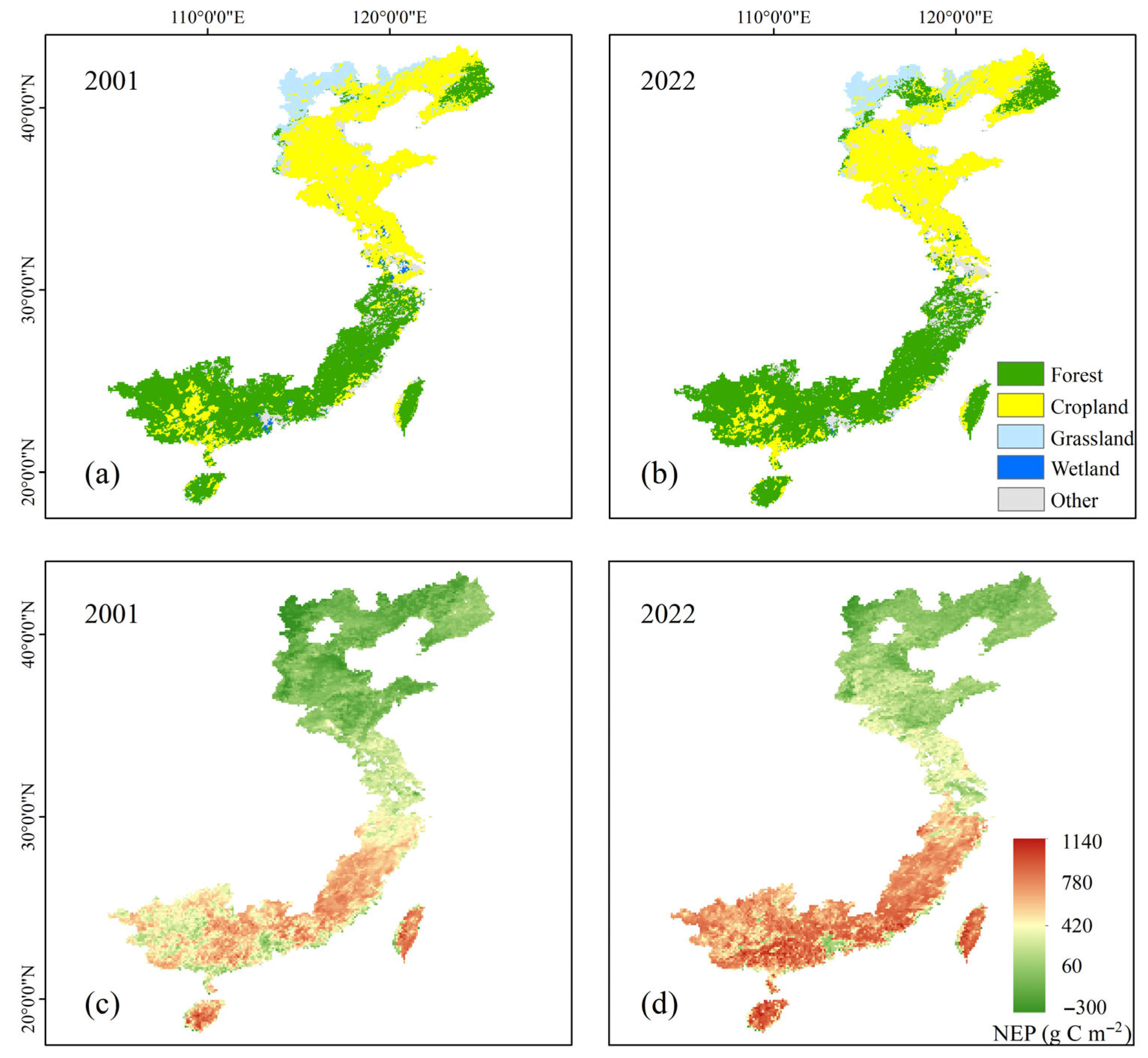
Eastern coastal China is an important region for terrestrial carbon exchange because of its high ecosystem productivity, strong monsoon influence, and substantial land cover changes. Changes in its carbon sink therefore have important implications for ecosystem functioning and the terrestrial carbon cycle at the national scale. From 2001 to 2022, NEP in eastern coastal China increased from 344.12 Tg C yr⁻¹ to 517.73 Tg C yr⁻¹, representing an overall increase of 50.45% (Figure 9 and Figure S4). The Sen’s slope estimator further indicated an increasing trend in regional total NEP, with a rate of 8.44 Tg C yr⁻² during 2001–2022. As a key indicator of ecosystem carbon sink strength, the sustained rise in NEP indicates that the net carbon uptake capacity of eastern coastal China generally strengthened over the study period. This result is consistent with previous studies showing an increase in terrestrial carbon sinks in China over recent decades, and further highlights the importance of the eastern monsoon region as a major carbon sink [2,56]. In addition, the CO₂ fertilization effect may have partly contributed to the sustained increase in regional NEP, because rising atmospheric CO₂ can enhance photosynthetic carbon uptake and improve plant water-use efficiency. However, as atmospheric CO₂ was not explicitly included as a predictor in this study, its contribution could not be quantified.

To evaluate the relationship between land cover change and regional carbon sink dynamics,

Table 9. Matrix of annual NEP changes associated with land-cover transitions from 2001 to 2022 (Tg C yr⁻¹).

Land Cover	Forest	Cropland	Grassland	Wetland	Other	Total
Forest	-	−5.14	−0.75	−0.03	−3.11	−9.03
Cropland	24.71	-	−0.80	0.14	0.11	24.16
Grassland	13.85	4.36	-	0.08	0.25	18.54
Wetland	1.20	−0.04	−0.10	-	0.03	1.09
Other	3.16	−0.01	−0.05	0.02	-	3.12
Total	42.92	−0.83	−1.70	0.21	−2.72	37.88

Note: Values indicate the changes in annual NEP due to land cover transitions from 2001 to 2022. Positive values represent increased NEP (enhanced carbon sink strength), while negative values indicate decreased NEP (weakened carbon sink strength). The row totals represent the net NEP changes for each land cover type in 2001, while the column totals represent the net NEP changes for each land cover type in 2022.

presents the annual NEP change matrix for areas undergoing land cover transitions from 2001 to 2022. Further details on land cover area transitions during this period are provided in Table S1. Overall, areas experiencing land cover transitions showed a net increase of approximately 37.88 Tg C yr⁻¹ in annual regional NEP, accounting for about 21.82% of the total regional NEP increase. This result suggests that land cover change was associated with an enhancement of the regional carbon sink, although the estimated NEP changes may also reflect the combined influence of climatic variability, vegetation dynamics, and other environmental factors. Therefore, these values should be interpreted as the NEP changes associated with land cover transitions rather than as the isolated causal effect of land cover change alone. Among different transition types, the positive NEP change was mainly observed in areas converted to forest, particularly cropland-to-forest and grassland-to-forest transitions, which were associated with increases of 24.71 and 13.85 Tg C yr⁻¹, respectively. In contrast, forest-to-cropland and forest-to-other-land transitions were associated with NEP decreases of 5.14 and 3.11 Tg C yr⁻¹, respectively. These results suggest that forest expansion was associated with enhanced regional carbon sink strength, whereas forest loss tended to weaken it.

As shown in

Table 10. Changes in NEP density and total NEP, and Sen’s slope of total NEP by land cover type from 2001 to 2022.

Land Cover	NEP Density in 2001 (g C m−2 yr−1)	NEP Density in 2022 (g C m−2 yr−1)	Total NEP in 2001 (Tg C yr−1)	Total NEP in 2022 (Tg C yr−1)	Change in Total NEP	Percent Change (%)	Total NEP Sen’s Slope (Tg C yr−2)
Forest	519.01	652.21	302.5	404.23	101.73	33.63	5.20 ***
Cropland	76.1	203.8	37.7	94.26	56.56	150.26	2.61 ***
Grassland	−111.57	−24.28	−10.6	−1.79	8.81	85.28	0.35 ***
Wetland	264.83	298.18	2.12	1.02	−1.1	−51.89	−0.03 **
Other	137.85	178.99	12.4	20.01	7.61	61.37	0.30 ***
Total	-	-	344.12	517.73	173.61	50.45	8.44 ***

Note: Sen’s slope was calculated from the annual time series during 2001–2022. *, **, and *** indicate significance at p < 0.05, p < 0.01, and p < 0.001, respectively.

, NEP trajectories differed markedly among land cover types during 2001–2022. Forests consistently dominated the regional carbon sink, with total NEP increasing from 302.50 to 404.23 Tg C yr⁻¹ between 2001 and 2022, representing an increase of 33.63%. The Sen’s slope of forest total NEP was 5.20 Tg C yr⁻², indicating a sustained increase in forest carbon uptake. These results confirm that forests were the principal contributor to both the magnitude and long-term enhancement of the regional carbon sink, consistent with previous studies showing that forests dominate China’s terrestrial carbon sink [56]. Croplands contributed less than forests in terms of total NEP, but they showed increases in both NEP density and total NEP. Total cropland NEP increased from 37.70 to 94.26 Tg C yr⁻¹, with a Sen’s slope of 2.61 Tg C yr⁻², suggesting an enhanced contribution to regional ecosystem-level carbon uptake. However, this increase should be interpreted cautiously because cropland NEP does not represent the full net carbon or greenhouse-gas balance of agricultural activities, which is also affected by crop harvest removal, management practices, crop types, irrigation, fertilization, and climatic variability. Grasslands showed a weakened carbon source effect, with total NEP increasing from −10.60 to −1.79 Tg C yr⁻¹. Although grasslands remained a net carbon source in 2022, the increase in NEP indicates that their carbon source effect weakened over time. Wetlands, in contrast, had a relatively high NEP density but declining total NEP, which decreased from 2.12 to 1.02 Tg C yr⁻¹. This pattern suggests that the relatively high per-area carbon sequestration capacity of wetlands was offset by wetland area loss, leading to a decline in their total contribution to regional carbon uptake.

Overall, land-cover transitions were associated with measurable changes in regional NEP, especially through forest-related conversions and wetland area reduction. However, these transition-associated NEP changes represented only part of the regional carbon sink enhancement, and the overall increase should be interpreted together with climatic variability, vegetation dynamics, and management influences.

4.3. Distinct Environmental Controls on GPP, ER, and NEP

Figure 4 reveals distinct dominant predictors for GPP, ER, and NEP, indicating that these carbon-cycle components were regulated by partly different environmental controls rather than by a single common set of drivers. This pattern is consistent with current ecological understanding and points to differentiated controls over individual carbon-cycle processes [57].

For GPP, the high importance of EVI, LSWI, and SIF suggests that its spatial variation was mainly associated with vegetation activity, water status, and photosynthetic functioning. This interpretation is ecologically reasonable because EVI and LSWI characterize canopy greenness and moisture conditions, whereas SIF more directly reflects photosynthetic activity. The SHAP summary plots further showed that higher values of these variables generally made positive contributions to GPP. Together, these results emphasize the dominant roles of vegetation condition and moisture availability in shaping spatial variation in GPP within the RF framework. For ER, EVI, T2M, and LSWI were the leading predictors, while EVAVT also contributed substantially. The SHAP summary plots showed that higher T2M values were generally associated with positive SHAP values, indicating that warmer conditions tended to enhance respiratory carbon release. At the same time, the dominant role of EVI and the additional contributions of LSWI and EVAVT suggest that ER was not governed by temperature alone, but was also strongly influenced by vegetation activity and moisture-related conditions. These findings indicate that spatial variation in ER reflected the combined influences of temperature, vegetation status, and water availability. For NEP, the dominant role of LSWI is particularly noteworthy, suggesting that moisture status exerted a stronger influence on net carbon balance than other environmental variables in the RF framework. Because NEP represents the balance between GPP and ER, its spatial pattern may reflect the integrated effects of water limitation on both carbon uptake and respiratory release. The higher importance of LSWI relative to VPD and PPT further suggests that NEP was more closely associated with surface or canopy moisture status than with atmospheric water demand or precipitation alone at this scale.

The relatively weak contributions of PPT, VPD, SSRD, and LAI_H should not be interpreted as evidence of ecological unimportance. To further evaluate the role of these lower-ranked predictors, we trained an RF model using only the five variables with the highest overall importance across the three flux components (EVAVT, T2M, EVI, LSWI, and SIF). This reduced model performed worse than the full model using all nine input variables in both validation and 10-fold cross-validation (Table 4, Table 5 and

Table 11. Performance of the reduced RF model using the five leading predictors under validation and 10-fold cross-validation.

Approach	Variable	R2		RMSE		MAE
		T	V	T	V	T	V
RF	GPP	0.96	0.91	0.70	1.10	0.49	0.82
	ER	0.93	0.83	0.56	0.98	0.41	0.70
	NEP	0.92	0.81	0.52	0.82	0.39	0.61
		MT	MV	MT	MV	MT	MV
RF-CV10	GPP	0.96	0.88	0.67	1.19	0.47	0.85
	ER	0.92	0.79	0.61	0.98	0.44	0.72
	NEP	0.92	0.75	0.52	0.91	0.38	0.70

Note: RF represents the model performance under optimal settings, while RF-CV10 denotes the 10-fold cross-validation results. T and V refer to the training and validation performance, respectively. MT and MV denote the mean training and validation performance across the 10 folds, respectively. The model used five predictors: EVAVT, T2M, EVI, LSWI, and SIF.

). Under 10-fold cross-validation, the validation R² values for GPP, ER, and NEP were 0.88, 0.79, and 0.75, respectively, and similar declines were also observed for RMSE and MAE. These results indicate that although the five leading predictors had very high feature importance, PPT, VPD, SSRD, and LAI_H also contributed to the model to some extent.

4.4. Management Implications and Research Perspectives

This study characterized the spatiotemporal patterns of GPP, ER, and NEP along the eastern coast of China from 2001 to 2022 and clarified the differing roles of ecosystem types in the regional carbon cycle.

Forests were identified as the dominant regional carbon sink, highlighting their importance for long-term carbon sequestration and the need for continued forest protection and ecological restoration. The increasing contribution of croplands indicates their important role in regional CO₂ uptake. However, this finding should be interpreted as an ecosystem-level NEP sink rather than evidence that agricultural activities as a whole act as a net carbon or greenhouse-gas sink, because harvest removal, management-related emissions, and crop-system differences were not explicitly considered. In contrast, although wetlands showed relatively high NEP per unit area, their declining total carbon sink indicates that wetland loss is weakening the contribution of these high-value coastal ecosystems to the regional carbon budget. Taken together, these findings suggest that future coastal carbon management should not rely solely on a single carbon-sink enhancement strategy. Instead, it should adopt a coordinated multi-ecosystem management framework that integrates forest conservation, agricultural optimization, and wetland restoration. Such an approach would help improve regional carbon-sink stability and support sustainable coastal ecosystem management.

From a carbon-cycle research perspective, the distinct dominant drivers of GPP, ER, and NEP indicate that these flux components should not be assumed to share a single common driver framework. Future studies should pay closer attention to the differential roles of vegetation condition, moisture status, and thermal constraints, and further examine how ecosystem type and land cover change jointly shape coastal carbon dynamics. The carbon flux dataset generated in this study also provides a scientific basis for long-term monitoring and regional comparisons of carbon cycle patterns along the eastern coast of China.

5. Conclusions

In this study, we developed a machine learning framework to estimate GPP, ER, and NEP along the eastern coast of China from 2001 to 2022. Flux tower observations, meteorological variables, remote sensing indices, and ecohydrological variables were used as input data for model development. Among the four evaluated approaches, the RF model showed the best overall performance. Its validation R² values were 0.92, 0.84, and 0.83 for GPP, ER, and NEP, respectively, and its performance remained generally good under both 10-fold cross-validation and leave-one-site-out cross-validation. The RF model also remained generally stable under single variable perturbation scenarios for all nine input predictors, indicating reasonable robustness to plausible input uncertainties during regional upscaling. Based on the optimal model, the eastern coast of China acted as a net carbon sink during 2001–2022, with mean GPP, ER, and NEP values of 1578.38, 1286.05, and 334.56 g C m⁻² yr⁻¹, respectively. All three flux components showed a clear south-to-north decreasing spatial gradient. Meanwhile, total regional NEP increased from 344.12 Tg C in 2001 to 517.73 Tg C in 2022, indicating a sustained enhancement of regional carbon-sink capacity. Forests remained the dominant contributor to the regional carbon sink, croplands showed an increasing contribution over time, and wetlands exhibited relatively high NEP per unit area but a declining total carbon sink due to area loss. Feature importance and SHAP analyses revealed distinct environmental controls on different carbon-flux components. EVI, LSWI, and SIF contributed most to GPP, whereas EVI, T2M, and LSWI were the leading predictors of ER, and LSWI exerted the strongest influence on NEP. These findings indicate that vegetation change and land cover dynamics were closely associated with the enhanced carbon sink along the eastern coast of China. They also provide scientific support for coordinated forest conservation, cropland management, and wetland restoration along the eastern coast of China.

However, several limitations should be acknowledged. First, although the RF model performed well under random cross-validation, the LOSO-CV results indicate that spatial extrapolation remains an important source of uncertainty. The lower LOSO-CV performance suggests that random cross-validation may overestimate model accuracy, while the site-dependent results further show that local environmental heterogeneity and uneven flux tower distribution can limit model transferability to unseen sites. This limitation was more evident for NEP than for GPP and ER. In particular, because the available flux towers did not include grassland sites, the model evaluation for grassland ecosystems relied on extrapolation from other ecosystem types. Although grasslands occupy a relatively small proportion of the study area and may therefore have limited influence on the overall regional estimates, the absence of grassland flux tower observations remains a limitation for interpreting grassland-specific NEP estimates. Second, the input variables mainly described vegetation, climate, and surface moisture conditions. Several other potentially important factors, including soil properties, belowground microbial activity, ecosystem management, and anthropogenic disturbances, were not explicitly considered. Third, feature importance and SHAP analyses improved model interpretability, but they mainly reflected statistical associations within the regional modeling framework. As a result, they may not fully capture differences in environmental controls among ecosystem types or across subregions. Future work could reduce these uncertainties by incorporating more flux observations from underrepresented regions and ecosystem types, as well as by integrating additional environmental and human-activity variables. Process-informed or hybrid approaches may also help improve model accuracy, generalizability, and mechanistic interpretability.

References

1. Wang, Y.; Wang, X.; Wang, K.; Chevallier, F.; Zhu, D.; Lian, J.; He, Y.; Tian, H.; Li, J.; Zhu, J.; et al. The Size of the Land Carbon Sink in China. Nature 2022, 603, E7–E9. [Google Scholar] [CrossRef] [PubMed]
2. Yu, Z.; Ciais, P.; Piao, S.; Houghton, R.A.; Lu, C.; Tian, H.; Agathokleous, E.; Kattel, G.R.; Sitch, S.; Goll, D.; et al. Forest Expansion Dominates China’s Land Carbon Sink since 1980. Nat. Commun. 2022, 13, 5374. [Google Scholar] [CrossRef] [PubMed]
3. Yue, C.; Xu, M.; Ciais, P.; Tao, S.; Shen, H.; Chang, J.; Li, W.; Deng, L.; He, J.; Leng, Y.; et al. Contributions of Ecological Restoration Policies to China’s Land Carbon Balance. Nat. Commun. 2024, 15, 9708. [Google Scholar] [CrossRef]
4. Liu, C.; Liu, D.; Li, P.; Li, X.; Liu, Z.; Zhao, Y. Assessment of Occupation of Natural Habitat by Urban Expansion and Its Impact on Crucial Ecosystem Services in China’s Coastal Zone. Ecol. Indic. 2023, 154, 110682. [Google Scholar] [CrossRef]
5. He, H.; Wang, S.; Zhang, L.; Wang, J.; Ren, X.; Zhou, L.; Piao, S.; Yan, H.; Ju, W.; Gu, F.; et al. Altered Trends in Carbon Uptake in China’s Terrestrial Ecosystems under the Enhanced Summer Monsoon and Warming Hiatus. Natl. Sci. Rev. 2019, 6, 505–514. [Google Scholar] [CrossRef]
6. Baldocchi, D.D. Assessing the Eddy Covariance Technique for Evaluating Carbon Dioxide Exchange Rates of Ecosystems: Past, Present and Future. Glob. Change Biol. 2003, 9, 479–492. [Google Scholar] [CrossRef]
7. Yu, G.; Chen, Z.; Piao, S.; Peng, C.; Ciais, P.; Wang, Q.; Li, X.; Zhu, X. High Carbon Dioxide Uptake by Subtropical Forest Ecosystems in the East Asian Monsoon Region. Proc. Natl. Acad. Sci. USA 2014, 111, 4910–4915. [Google Scholar] [CrossRef]
8. Gao, S.; Hou, X.-H.; Wang, Y.; Wang, Q.; Chen, Y.; Xing, R.; Wang, J. Remote Sensing Monitoring of Terrestrial Ecosystem Carbon Budget based on Machine Learning and Big Data Platform. Remote Sens. Technol. Appl. 2022, 37, 1190–1197. [Google Scholar] [CrossRef]
9. Wang, J.; Yu, G.; Han, L.; Yao, Y.; Sun, M.; Yan, Z. Ecosystem Carbon Exchange across China’s Coastal Wetlands: Spatial Patterns, Mechanisms, and Magnitudes. Agric. For. Meteorol. 2024, 345, 109859. [Google Scholar] [CrossRef]
10. You, C.; Wang, Y.; Tan, X.; Cui, E.; Zhang, B.; Bian, C.; Chen, B.; Xu, M.; Han, X.; Xia, J.; et al. Inner Mongolia Grasslands Act as a Weak Regional Carbon Sink: A New Estimation Based on Upscaling Eddy Covariance Observations. Agric. For. Meteorol. 2023, 342, 109719. [Google Scholar] [CrossRef]
11. Shahan, J.; Chu, H.; Windham-Myers, L.; Matsumura, M.; Carlin, J.; Eichelmann, E.; Stuart-Haentjens, E.; Bergamaschi, B.; Nakatsuka, K.; Sturtevant, C.; et al. Combining Eddy Covariance and Chamber Methods to Better Constrain CO2 and CH4 Fluxes Across a Heterogeneous Restored Tidal Wetland. J. Geophys. Res. Biogeosci. 2022, 127, e2022JG007112. [Google Scholar] [CrossRef]
12. Baldocchi, D.D. How Eddy Covariance Flux Measurements Have Contributed to Our Understanding of Global Change Biology. Glob. Change Biol. 2020, 26, 242–260. [Google Scholar] [CrossRef] [PubMed]
13. Lasslop, G.; Reichstein, M.; Papale, D.; Richardson, A.D.; Arneth, A.; Barr, A.; Stoy, P.; Wohlfahrt, G. Separation of Net Ecosystem Exchange into Assimilation and Respiration Using a Light Response Curve Approach: Critical Issues and Global Evaluation. Glob. Change Biol. 2010, 16, 187–208. [Google Scholar] [CrossRef]
14. Reichstein, M.; Falge, E.; Baldocchi, D.; Papale, D.; Aubinet, M.; Berbigier, P.; Bernhofer, C.; Buchmann, N.; Gilmanov, T.; Granier, A.; et al. On the Separation of Net Ecosystem Exchange into Assimilation and Ecosystem Respiration: Review and Improved Algorithm. Glob. Change Biol. 2005, 11, 1424–1439. [Google Scholar] [CrossRef]
15. Baldocchi, D.; Penuelas, J. The Physics and Ecology of Mining Carbon Dioxide from the Atmosphere by Ecosystems. Glob. Change Biol. 2019, 25, 1191–1197. [Google Scholar] [CrossRef]
16. Running, S.W.; Nemani, R.R.; Heinsch, F.A.; Zhao, M.; Reeves, M.; Hashimoto, H. A Continuous Satellite-Derived Measure of Global Terrestrial Primary Production. BioScience 2004, 54, 547–560. [Google Scholar] [CrossRef]
17. Krinner, G.; Viovy, N.; de Noblet-Ducoudré, N.; Ogée, J.; Polcher, J.; Friedlingstein, P.; Ciais, P.; Sitch, S.; Prentice, I.C. A Dynamic Global Vegetation Model for Studies of the Coupled Atmosphere-Biosphere System. Glob. Biogeochem. Cycles 2005, 19, GB1015. [Google Scholar] [CrossRef]
18. Lawrence, D.M.; Fisher, R.A.; Koven, C.D.; Oleson, K.W.; Swenson, S.C.; Bonan, G.; Collier, N.; Ghimire, B.; van Kampenhout, L.; Kennedy, D.; et al. The Community Land Model Version 5: Description of New Features, Benchmarking, and Impact of Forcing Uncertainty. J. Adv. Model. Earth Syst. 2019, 11, 4245–4287. [Google Scholar] [CrossRef]
19. Smith, B.; Prentice, I.C.; Sykes, M.T. Representation of Vegetation Dynamics in the Modelling of Terrestrial Ecosystems: Comparing Two Contrasting Approaches within European Climate Space. Glob. Ecol. Biogeogr. 2001, 10, 621–637. [Google Scholar] [CrossRef]
20. Intergovernmental Panel on Climate Change (IPCC) (Ed.) Carbon and Other Biogeochemical Cycles. In Climate Change 2013—The Physical Science Basis: Working Group I Contribution to the Fifth Assessment Report of the Intergovernmental Panel on Climate Change; Cambridge University Press: Cambridge, UK, 2014; pp. 465–570.
21. Jung, M.; Reichstein, M.; Margolis, H.A.; Cescatti, A.; Richardson, A.D.; Arain, M.A.; Arneth, A.; Bernhofer, C.; Bonal, D.; Chen, J.; et al. Global Patterns of Land-Atmosphere Fluxes of Carbon Dioxide, Latent Heat, and Sensible Heat Derived from Eddy Covariance, Satellite, and Meteorological Observations. J. Geophys. Res. Biogeosci. 2011, 116, G00J07. [Google Scholar] [CrossRef]
22. Yu, G.-R.; Zhu, X.-J.; Fu, Y.-L.; He, H.-L.; Wang, Q.-F.; Wen, X.-F.; Li, X.-R.; Zhang, L.-M.; Zhang, L.; Su, W.; et al. Spatial Patterns and Climate Drivers of Carbon Fluxes in Terrestrial Ecosystems of China. Glob. Change Biol. 2013, 19, 798–810. [Google Scholar] [CrossRef] [PubMed]
23. Ngoc Tu, N.; Lü, H.; He, W.; Xu, P.; Zhao, M.; Liu, S.; Zhu, Y.; Lei, X. Automated Machine Learning Integrating Multi-Source Satellite Observations to Predict Gross and Net CO2 Fluxes of Coastal Wetlands in China. Environ. Res. Lett. 2025, 20, 084011. [Google Scholar] [CrossRef]
24. Nguyen, N.T.; Lü, H.; He, W.; Ma, T.; Yang, H.; Xu, P.; Liu, S.; Zhao, M.; Zhu, Y. Modeling CO2 Fluxes in Coastal Wetlands of China Using Explainable Sequence-Based Deep Learning. Ecol. Inform. 2026, 95, 103766. [Google Scholar] [CrossRef]
25. Xiao, X.; Hollinger, D.; Aber, J.; Goltz, M.; Davidson, E.A.; Zhang, Q.; Moore, B. Satellite-Based Modeling of Gross Primary Production in an Evergreen Needleleaf Forest. Remote Sens. Environ. 2004, 89, 519–534. [Google Scholar] [CrossRef]
26. He, B.; Chen, C.; Lin, S.; Yuan, W.; Chen, H.W.; Chen, D.; Zhang, Y.; Guo, L.; Zhao, X.; Liu, X.; et al. Worldwide Impacts of Atmospheric Vapor Pressure Deficit on the Interannual Variability of Terrestrial Carbon Sinks. Natl. Sci. Rev. 2022, 9, nwab150. [Google Scholar] [CrossRef]
27. Running, S.W.; Thornton, P.E.; Nemani, R.; Glassy, J.M. Global Terrestrial Gross and Net Primary Productivity from the Earth Observing System. In Methods in Ecosystem Science; Sala, O.E., Jackson, R.B., Mooney, H.A., Howarth, R.W., Eds.; Springer: New York, NY, USA, 2000; pp. 44–57. [Google Scholar]
28. Zeng, J.; Matsunaga, T.; Tan, Z.-H.; Saigusa, N.; Shirai, T.; Tang, Y.; Peng, S.; Fukuda, Y. Global Terrestrial Carbon Fluxes of 1999–2019 Estimated by Upscaling Eddy Covariance Data with a Random Forest. Sci. Data 2020, 7, 313. [Google Scholar] [CrossRef]
29. Rozanov, A.P.; Gribanov, K.G. A Neural Network Model for Estimating Carbon Fluxes in Forest Ecosystems from Remote Sensing Data. Atmos. Ocean. Opt. 2023, 36, 323–328. [Google Scholar] [CrossRef]
30. Han, Y.; Han, Z. Vegetation Carbon Source/Sink Dynamics and Extreme Climate Response in the Yangtze River Delta Coastal Zone. Sustainability 2025, 17, 1456. [Google Scholar] [CrossRef]
31. Zhao, H.; Fan, J.; Gu, B.; Chen, Y. Carbon Sink Response of Terrestrial Vegetation Ecosystems in the Yangtze River Delta and Its Driving Mechanism. J. Geogr. Sci. 2024, 34, 112–130. [Google Scholar] [CrossRef]
32. Kang, J.; Zhang, B.; Dang, A. A Novel Geospatial Machine Learning Approach to Quantify Non-Linear Effects of Land Use/Land Cover Change (LULCC) on Carbon Dynamics. Int. J. Appl. Earth Obs. Geoinf. 2024, 128, 103712. [Google Scholar] [CrossRef]
33. Katzenberger, A.; Levermann, A. Consistent Increase in East Asian Summer Monsoon Rainfall and Its Variability under Climate Change over China in CMIP6. Earth Syst. Dyn. 2024, 15, 1137–1151. [Google Scholar] [CrossRef]
34. Sun, R.-H.; Li, Z.; Chen, L.-D. Review of ecological regionalization and classification in China: Ecological patterns, functions, and ecosystem services. Acta Ecol. Sin. 2018, 38, 5271–5278. [Google Scholar] [CrossRef]
35. Chen, M.; Li, M.; Wang, P. Spatiotemporal Patterns and Dynamic Mechanisms of Ecosystem Services in the Coastal Zone of China. Front. Environ. Sci. 2025, 13, 1506136. [Google Scholar] [CrossRef]
36. He, H.; Liu, M.; Sun, X.; Zhang, L.; Luo, Y.; Wang, H.; Han, S.; Zhao, X.; Shi, P.; Wang, Y.; et al. Uncertainty Analysis of Eddy Flux Measurements in Typical Ecosystems of ChinaFLUX. Ecol. Inform. 2010, 5, 492–502. [Google Scholar] [CrossRef]
37. Isaac, P.; Cleverly, J.; McHugh, I.; van Gorsel, E.; Ewenz, C.; Beringer, J. OzFlux Data: Network Integration from Collection to Curation. Biogeosciences 2017, 14, 2903–2928. [Google Scholar] [CrossRef]
38. Muñoz-Sabater, J.; Dutra, E.; Agustí-Panareda, A.; Albergel, C.; Arduini, G.; Balsamo, G.; Boussetta, S.; Choulga, M.; Harrigan, S.; Hersbach, H.; et al. ERA5-Land: A State-of-the-Art Global Reanalysis Dataset for Land Applications. Earth Syst. Sci. Data 2021, 13, 4349–4383. [Google Scholar] [CrossRef]
39. Allen, R.G.; Pereira, L.S.; Raes, D.; Smith, M. Crop Evapotranspiration: Guidelines for Computing Crop Water Requirements; FAO Irrigation and Drainage Paper; Food and Agriculture Organization of the United Nations: Rome, Italy, 1998. [Google Scholar]
40. He, J.; Yang, K.; Tang, W.; Lu, H.; Qin, J.; Chen, Y.; Li, X. The First High-Resolution Meteorological Forcing Dataset for Land Process Studies over China. Sci. Data 2020, 7, 25. [Google Scholar] [CrossRef]
41. Tao, S.; Chen, J.M.; Zhang, Z.; Zhang, Y.; Ju, W.; Zhu, T.; Wu, L.; Wu, Y.; Kang, X. A High-Resolution Satellite-Based Solar-Induced Chlorophyll Fluorescence Dataset for China from 2000 to 2022. Sci. Data 2024, 11, 1286. [Google Scholar] [CrossRef]
42. Jung, M.; Schwalm, C.; Migliavacca, M.; Walther, S.; Camps-Valls, G.; Koirala, S.; Anthoni, P.; Besnard, S.; Bodesheim, P.; Carvalhais, N.; et al. Scaling Carbon Fluxes from Eddy Covariance Sites to Globe: Synthesis and Evaluation of the FLUXCOM Approach. Biogeosciences 2020, 17, 1343–1365. [Google Scholar] [CrossRef]
43. Tramontana, G.; Jung, M.; Schwalm, C.R.; Ichii, K.; Camps-Valls, G.; Ráduly, B.; Reichstein, M.; Arain, M.A.; Cescatti, A.; Kiely, G.; et al. Predicting Carbon Dioxide and Energy Fluxes across Global FLUXNET Sites with Regression Algorithms. Biogeosciences 2016, 13, 4291–4313. [Google Scholar] [CrossRef]
44. Ma, H.; Liu, S. The Potential Evaluation of Multisource Remote Sensing Data for Extracting Soil Moisture Based on the Method of BP Neural Network. Can. J. Remote Sens. 2016, 42, 117–124. [Google Scholar] [CrossRef]
45. Hu, H.; Song, Y.; Yu, J.; Liu, Y.; Chen, F. The Application of Support Vector Regression and Virtual Sample Generation Technique in the Optimization Design of Transonic Compressor. Aerosp. Sci. Technol. 2022, 130, 107814. [Google Scholar] [CrossRef]
46. Chen, L.; Xing, M.; He, B.; Wang, J.; Shang, J.; Huang, X.; Xu, M. Estimating Soil Moisture over Winter Wheat Fields During Growing Season Using Machine-Learning Methods. IEEE J. Sel. Top. Appl. Earth Obs. Remote Sens. 2021, 14, 3706–3718. [Google Scholar] [CrossRef]
47. Adnan, R.M.; Mirboluki, A.; Mehraein, M.; Malik, A.; Heddam, S.; Kisi, O. Improved Prediction of Monthly Streamflow in a Mountainous Region by Metaheuristic-Enhanced Deep Learning and Machine Learning Models Using Hydroclimatic Data. Theor. Appl. Climatol. 2024, 155, 205–228. [Google Scholar] [CrossRef]
48. Pantic, I.V.; Paunovic Pantic, J.; Valjarevic, S.; Corridon, P.R.; Topalovic, N. Artificial Intelligence—Based Approaches Based on Random Forest Algorithm for Signal Analysis: Potential Applications in Detection of Chemico—Biological Interactions. Chem. Biol. Interact. 2025, 418, 111624. [Google Scholar] [CrossRef]
49. Chen, T.; Guestrin, C. XGBoost: A Scalable Tree Boosting System. In Proceedings of the 22nd ACM SIGKDD International Conference on Knowledge Discovery and Data Mining; Association for Computing Machinery: New York, NY, USA, 2016; pp. 785–794. [Google Scholar]
50. Ribeiro, M.H.D.M.; dos Santos Coelho, L. Ensemble Approach Based on Bagging, Boosting and Stacking for Short-Term Prediction in Agribusiness Time Series. Appl. Soft Comput. 2020, 86, 105837. [Google Scholar] [CrossRef]
51. Yu, S.; Song, Z.; Bai, Y.; Guo, X.; He, X.; Zhai, W.; Zhao, H.; Dai, M. Satellite-Estimated Air-Sea CO2 Fluxes in the Bohai Sea, Yellow Sea, and East China Sea: Patterns and Variations during 2003–2019. Sci. Total Environ. 2023, 904, 166804. [Google Scholar] [CrossRef]
52. Vega García, M.; Aznarte, J.L. Shapley Additive Explanations for NO2 Forecasting. Ecol. Inform. 2020, 56, 101039. [Google Scholar] [CrossRef]
53. Lundberg, S.M.; Lee, S.-I. A Unified Approach to Interpreting Model Predictions. In Proceedings of the 31st International Conference on Neural Information Processing Systems; Curran Associates Inc.: Red Hook, NY, USA, 2017; pp. 4768–4777. [Google Scholar]
54. Nelson, J.A.; Walther, S.; Gans, F.; Kraft, B.; Weber, U.; Novick, K.; Buchmann, N.; Migliavacca, M.; Wohlfahrt, G.; Šigut, L.; et al. X-BASE: The First Terrestrial Carbon and Water Flux Products from an Extended Data-Driven Scaling Framework, FLUXCOM-X. Biogeosciences 2024, 21, 5079–5115. [Google Scholar] [CrossRef]
55. Liu, F. Research on Carbon Flux and Energy Exchange in a Subtropical Mangrove Ecosystem. Master’s Thesis, Tsinghua University, Beijing, China, 2015. [Google Scholar]
56. Yang, Y.; Shi, Y.; Sun, W.; Chang, J.; Zhu, J.; Chen, L.; Wang, X.; Guo, Y.; Zhang, H.; Yu, L.; et al. Terrestrial Carbon Sinks in China and around the World and Their Contribution to Carbon Neutrality. Sci. China Life Sci. 2022, 65, 861–895. [Google Scholar] [CrossRef]
57. Kira, O.; Chang, C.Y.-Y.; Gu, L.; Wen, J.; Hong, Z.; Sun, Y. Partitioning Net Ecosystem Exchange (NEE) of CO2 Using Solar-Induced Chlorophyll Fluorescence (SIF). Geophys. Res. Lett. 2021, 48, e2020GL091247. [Google Scholar] [CrossRef]
Figure 1. Spatial distribution of the study area along the eastern coast of China: (a) elevation (m) and locations of flux tower sites; (b) dominant land cover types across the study region.
Remotesensing 18 01580 g001
Figure 2. Comparison of environmental variable ranges between 2001 and 2005 and the flux-tower training samples. Violin plots show the distributions of the nine input variables used in the RF model, including T2M, PPT, VPD, EVI, LSWI, LAI_H, EVAVT, SIF, and SSRD. EVR represents the environmental variable range during 2001–2005, and SEVR represents the environmental variable range covered by the flux-tower training samples.
Remotesensing 18 01580 g002
Figure 3. Scatter plots of observed versus predicted GPP, ER, and NEP for the training and testing sets based on the optimal RF model. (ac) show the scatter plots for GPP, ER, and NEP, respectively.
Remotesensing 18 01580 g003
Figure 4. SHAP importance rankings and summary plots of environmental predictors for GPP, ER, and NEP based on the RF model. (ac) show the mean absolute SHAP values of predictors for GPP, ER, and NEP, respectively; (df) show the corresponding SHAP summary plots. Colors indicate feature values from low to high.
Remotesensing 18 01580 g004
Figure 5. Spatial patterns of annual average carbon fluxes GPP (a), ER (b), NEP (c) and CUE (d) along the eastern coast of China from 2001 to 2022.
Remotesensing 18 01580 g005
Figure 6. Interannual variations in annual average carbon fluxes GPP, ER, and NEP along the eastern coast of China from 2001 to 2022.
Remotesensing 18 01580 g006
Figure 7. Comparison of the spatial distributions of mean annual GPP, ER, and NEP between RF estimates and the FLUXCOM-X-BASE product along the eastern coast of China from 2001 to 2021. Panels (a,c,e) show the spatial distributions of GPP, ER, and NEP estimated by the RF model, respectively, whereas panels (b,d,f) show the corresponding results from FLUXCOM-X-BASE.
Remotesensing 18 01580 g007
Figure 8. Comparison of interannual variations in GPP, ER, and NEP between RF estimates and the FLUXCOM-X-BASE product along the eastern coast of China from 2001 to 2021. Panels (ac) show the interannual variations in GPP, ER, and NEP, respectively. *, **, and *** indicate significance at p < 0.05, p < 0.01, and p < 0.001, respectively.
Remotesensing 18 01580 g008
Figure 9. Spatial distribution of land cover types and NEP in the eastern coastal region of China in 2001 and 2022. (a,b) show land cover types in 2001 and 2022, respectively; (c,d) show the corresponding spatial patterns of NEP.
Remotesensing 18 01580 g009