


Highlights
What are the main findings?
- SITS benchmark datasets have transitioned from single-sensor, small-scale samples to multi-modal, global-scale datasets.
- Irregular sampling, cloud occlusion, and inconsistent label taxonomies are identified as the primary bottlenecks for model universality.
What are the implications of the main findings?
- Future research should prioritize multi-source and reconcile the trade-offs between high-temporal and high-spatial resolutions.
- Generative models and self-supervised foundation models represent the essential paradigm shift for reconstructing cloud-contaminated data and overcoming labeling scarcity.
Abstract
Recent advances in satellite missions, particularly the Landsat, Sentinel, and Gaofen series, have led to the rapid accumulation of high-quality remote sensing data with frequent revisits. As these data have become more widely available, Satellite Image Time Series (SITS) have become an important tool for monitoring Earth surface dynamics. SITS now supports a wide range of applications, including precision agriculture, Land Use/Cover Change (LULCC) monitoring, environmental management, and disaster response. This growth has also promoted the development of advanced SITS classification datasets. However, existing reviews have mainly focused on SITS classification algorithms or specific applications, while systematic comparisons of public SITS benchmark datasets remain limited. This lack of synthesis makes it difficult for researchers to navigate fragmented resources and select datasets that match specific scientific or operational tasks. To address this gap, this paper provides a comprehensive review and analysis of 29 publicly available medium-to-high-resolution SITS classification benchmark datasets released between 2017 and 2025. These datasets are intended for training, testing, and validating land-cover classification algorithms, rather than for direct use as operational map products. We conduct a detailed statistical and comparative analysis of these datasets, focusing on their key characteristics across spectral, temporal, and spatial dimensions, as well as their labeling systems. In addition, this review summarizes the SITS classification algorithms that have been developed and benchmarked using these datasets. Finally, we identify the main challenges in constructing and applying SITS classification datasets and discuss future research directions, particularly in data reconstruction, multimodal fusion, change analysis, and advanced model architectures. This survey provides the research community with a systematic overview of SITS classification benchmark datasets and aims to support continued progress in this rapidly developing field.
1. Introduction
Understanding Earth surface processes requires continuous spatio-temporal observations, which single-date imagery cannot provide. Satellite Image Time Series (SITS), which consist of chronologically ordered images of the same area, address this limitation by recording temporal dynamics that are needed to interpret surface changes. This temporal information helps distinguish land-cover types that may appear spectrally similar in isolated images. In Figure 1, panel (a) shows how SITS can represent urban expansion, seasonal vegetation phenology, and rapid disaster events, while panel (b) presents characteristic NDVI trajectories for different land-cover and crop categories [1]. In precision agriculture, SITS acquired over the full growing season support crop-type classification, crop health monitoring, phenology tracking, stress detection, and yield prediction [2]. These applications inform more targeted planting decisions, yield forecasting, and fine-scale management of irrigation and fertilization [3,4,5]. For Land Use/Cover Change (LULCC) analysis, SITS help detect gradual trends and abrupt transitions, including urban sprawl, deforestation, wetland loss, and agricultural land conversion. These observations provide useful evidence for spatial planning and resource management [6,7,8]. In environmental monitoring, SITS are used to assess vegetation responses to climate change, including shifts in greening and senescence, changes in the extent and condition of water bodies, and glacier retreat [9,10,11]. For disaster response, SITS enable rapid mapping of flood dynamics, support damage and recovery assessment after earthquakes or wildfires, and provide critical spatio-temporal information for emergency planning and relief operations [12,13,14]. These capabilities are difficult to achieve with single-date static imagery.
Figure 1.
Illustrative SITS. (a) Examples across different temporal scales: multi-year urban expansion, annual vegetation cycles, and rapid disaster dynamics. (b) Time-series profiles of NDVI for typical land-cover and crop types, illustrating distinct phenological patterns. Different colored lines represent the NDVI temporal profiles of different land-cover and crop types.
Recent advances in Earth observation satellite technology, supported by public satellite programs such as Landsat, Sentinel, and Gaofen and by commercial microsatellite constellations such as PlanetScope [15], have greatly increased the availability of high-quality remote sensing data with frequent global revisits [16]. This increase has promoted the development of SITS classification benchmark datasets, which provide an important basis for training, validating, and evaluating SITS classification algorithms. In earlier periods, acquiring SITS data with both high temporal frequency and fine spatial detail was difficult because the number of Earth observation satellites was limited. Many studies therefore relied on sensors with moderate or coarse spatial resolution, such as MODIS, and focused on specific applications, including crop classification and forest change detection [17,18]. Recent multi-satellite constellations have changed this situation. For example, Sentinel-2 provides observations with improved spatial and temporal resolution, including a 10 m spatial resolution and a 5-day revisit cycle [16]. These advances have supported a broader range of applications, including multi-crop mapping and dynamic urban monitoring.
However, the wider availability of richer data has not removed the difficulty of building SITS classification benchmark datasets. Large data volumes have to be managed while maintaining consistent geographic coverage, accurate geometric alignment, and reliable radiometric quality. These requirements place heavy demands on data collection, storage, preprocessing, and labeling. Multi-temporal observations are also often affected by clouds and atmospheric conditions, which can leave gaps in the time series. Irregular acquisition schedules may further lead to non-uniform temporal sampling and temporal phase misalignment. These dataset-level issues continue to constrain the development of modern SITS classification methods [19].
Current research on SITS classification therefore aims to improve dataset quality and usability, while also developing algorithms that can process complex time-series data. Important directions include data reconstruction and inpainting to reduce cloud effects, multi-sensor fusion to improve spatio-temporal resolution, and the construction of standardized, diverse, and challenging benchmark datasets for SITS classification. At the algorithmic level, recent methods increasingly account for irregular sampling and variable sequence lengths, improve robustness to abrupt contamination from clouds and shadows, extract information more efficiently from high-dimensional inputs, and seek a better balance between computational cost and accuracy, including through lightweight models [20,21].
Over the last several years, several high-quality SITS classification datasets have been released, despite continuing challenges in data acquisition, preprocessing, and annotation. These datasets have helped advance SITS classification by supporting model training, validation, and comparative evaluation. However, existing reviews have mainly focused on classification algorithms, specific application domains, or general remote sensing time-series analysis [1]. A systematic synthesis of public SITS classification datasets remains limited [22]. In particular, prior reviews have not compared these datasets in detail in terms of sensor configurations, temporal sampling strategies, spatial resolutions, spectral information, label taxonomies, data accessibility, and evaluation protocols. This gap makes it difficult for researchers to select suitable datasets, interpret benchmark results, and conduct fair and reproducible comparisons across studies [23,24].
To support appropriate dataset selection, SITS benchmark datasets should be distinguished from land-cover map products. SITS benchmark datasets provide temporal sensor observations and reference labels for training, validation, and testing classification models, and they are the main focus of this review. By contrast, land-cover map products are large-scale mapping outputs, such as GLASS-GLC [25], GLC_FCS30D [26], YRCC_LPLC [27], GLC_FC10 [28], and the 30 m annual China Land Cover Dataset [29]. Although these products may be used as label sources or validation references in model development, they are not reviewed as benchmark datasets in this paper.
To fill this gap, this paper provides a systematic review of 29 publicly available SITS classification benchmark datasets. Section 2 introduces these datasets and groups them by sensor type. Section 3 analyzes their key characteristics in terms of temporal and spatial resolution, spectral information, and labeling schemes. Section 4 reviews SITS classification algorithms that have been developed for, or evaluated on, these datasets. Section 5 discusses current challenges in SITS datasets and outlines future research directions. Finally, Section 6 concludes the paper.
2. Satellite Image Time Series Classification Benchmark Datasets
We identified and reviewed 29 publicly available medium- to high-resolution SITS classification benchmark datasets released between 2017 and 2025. Table 1 summarizes their spectral bands and sensor configurations. These datasets draw on major remote sensing data sources, including Sentinel-1, Sentinel-2, Landsat, Gaofen, Google Earth imagery, aerial imagery, PlanetScope, and MODIS products. This section first describes the dataset collection procedure and selection criteria, and then summarizes the reviewed datasets by sensor type.
2.1. Dataset Collection and Selection Criteria
To make the dataset inventory transparent and reproducible, we set the inclusion and exclusion criteria before conducting the review. We included a dataset only when it was publicly accessible, provided satellite image time series or multi-temporal remote sensing observations, contained categorical reference labels for thematic classification tasks such as land-cover, crop-type, vegetation-type, or tree-species mapping, and was designed for, or commonly used in, model training, validation, testing, or benchmark comparison. We also required documentation on sensor sources, temporal coverage, spatial resolution, label classes, and data splits that was sufficient to support reproducible use.
Resources outside this scope were excluded. These included operational land-cover products released only as final thematic maps, single-date scene classification datasets, non-public datasets, datasets without categorical reference labels, products intended primarily for regression or biophysical-parameter retrieval, and resources for which access or reuse could not be adequately verified. Duplicate releases and updated versions of the same dataset were treated as a single dataset when they used the same source data and followed the same benchmark protocol.
The final set of 29 datasets was selected to cover the main types of public SITS classification benchmarks released between 2017 and 2025. These datasets vary in sensor configuration, spatial resolution, temporal sampling strategy, geographic region, label taxonomy, and application setting, including land-cover classification, crop-type mapping, and tree-species classification. They therefore provide a representative overview of current public SITS benchmark resources, rather than a catalogue of operational land-cover map products.
2.2. Single-Sensor Datasets
2.2.1. Sentinel-2
As shown in Figure 2, 12 of the reviewed datasets are based only on Sentinel-2 imagery, most commonly at a 10 m spatial resolution, as reported in Table 1. Early European examples include the crop-type datasets released by Rußwurm et al. in 2017 and 2018 [30,31]. These datasets focus on agricultural areas north of Munich, Germany, and contain multi-band time series with parcel-level crop labels covering 17–19 classes for classification tasks. In 2020, BreizhCrops extended parcel-level crop mapping to the Brittany region of France using all Sentinel-2 bands for crop classification [32]. LandCoverNet, also released in 2020, covers several global regions and provides labeled image chips for annual land-cover model training across multiple classes [33].
Several European Sentinel-2 datasets released in 2021 further broadened the scope of crop classification. TimeSen2Crop covers Austria with one-year time series, pixel- or parcel-level crop labels, and cloud and shadow flags for classification [34]. ZurichCrops focuses on parts of Switzerland and provides similar pixel- or parcel-level crop classes for agricultural mapping [35]. PASTIS contains long sequences from four tiles in France, with pixel-level labels for semantic segmentation across crop classes [36]. EUROCROPS brings together agricultural parcel data from several European countries and uses hierarchical HCAT-ID labels for multi-level crop classification [37]. Sen4AgriNet combines multi-year imagery with LPIS labels across Europe and follows extended FAO ICC classes for crop identification and segmentation [38].
Datasets released from 2022 onward further expanded the temporal and spatial design of Sentinel-2 benchmarks in Europe. T31TFM-1618 updates the French coverage for 2016–2018 and provides parcel-level crop classes for annual classification using fixed-size patches [39]. AgriSen-COG covers Central Europe and uses FAO ICC labels for pixel- and parcel-level crop-type mapping at 10 m resolution [40]. The 2024 benchmark released by Rußwurm and Körner covers Bavaria, Germany, and provides seven major land-cover classes for irregular time-series classification during the 2016 vegetation period [41].
2.2.2. Planet
DynamicEarthNet [42] is a PlanetScope-based dataset developed for high-frequency change detection and semantic segmentation. It covers 75 regions worldwide during 2018–2019 and provides daily 3 m multispectral imagery. Pixel-level labels are provided once per month, producing dense time series with seven land-use and land-cover classes.
2.2.3. Landsat
TiSeLaC [43] is a Landsat-8-based dataset with a 30 m spatial resolution, covering Réunion Island in 2014. It provides pixel-level labels for nine land-cover classes and is mainly used for land-cover classification. Hankui Zhang et al. [44] released a 30 m dataset built from Landsat 5, 7, and 8 imagery for the conterminous United States. The dataset contains pixel-level land-cover labels for three epochs, 1985, 2006, and 2018, and supports long-term classification and change analysis.
2.2.4. Gaofen
This review also includes 3DFGC [45], a 4 m resolution benchmark covering Anqiu City, China, in 2015 and 2017. It provides pixel-level annotations for fine-grained crop types and was designed to support spatio-temporal deep learning research.
Table 1.
Spectral bands and data availability of the datasets.
Figure 2.
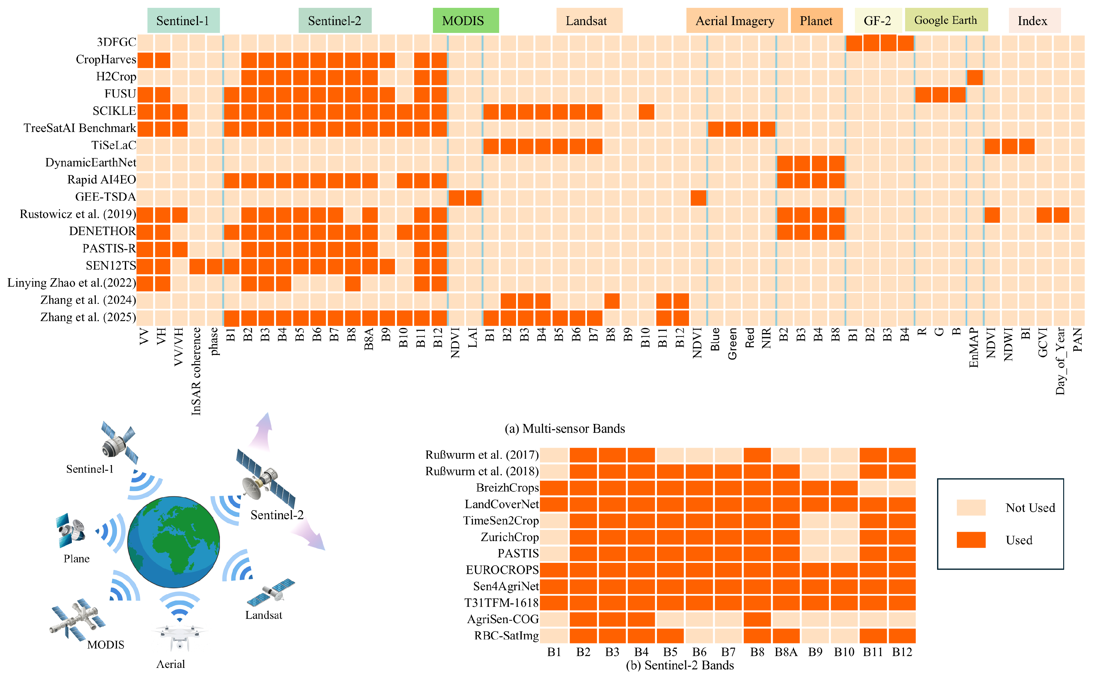
Summary of spectral band utilization across SITS classification benchmark datasets. (a) Band selection of datasets that integrate data from multiple platforms (e.g., Sentinel-1, Sentinel-2, MODIS, and Landsat). (b) Detailed breakdown of spectral band selection in datasets relying exclusively on Sentinel-2 imagery. The author–year source labels shown in the figure body correspond to Rußwurm et al. (2017) [30], Rußwurm et al. (2018) [31], Rustowicz et al. (2019) [47], Linying Zhao et al. (2022) [53], Zhang et al. (2024) [44], and Zhang et al. (2025) [56].
2.3. Multi-Sensor Datasets
Multi-sensor SITS benchmark datasets combine complementary observations from different platforms and sensors. They generally follow three forms of integration. Some datasets combine optical and SAR data, most often Sentinel-2 and Sentinel-1, to improve robustness under cloud contamination and to include structural information from radar backscatter. Others combine sensors with different spatial or temporal resolutions, such as Sentinel-2 with PlanetScope, Landsat, MODIS, or aerial imagery, to increase temporal density or spatial detail. A further group links multispectral data with sources that provide richer spectral or contextual information, including hyperspectral, aerial, or Google Earth imagery, for fine-grained crop, tree-species, or urban land-use classification. These datasets improve information completeness, but they also introduce technical difficulties related to geometric co-registration, radiometric harmonization, temporal alignment, and label consistency.
2.3.1. Sentinel-1 and Sentinel-2
PASTIS-R [49], SEN12TS [52], CropHarvest [48], and the dataset released by Linying Zhao et al. [53] combine Sentinel-2 optical imagery with Sentinel-1 SAR data to use complementary spectral and structural information. This pairing is particularly useful in cloudy regions, where SAR observations can preserve data coverage when optical imagery is missing or degraded. PASTIS-R extends the original PASTIS dataset by adding dense Sentinel-1 time series for 2019. SEN12TS provides paired Sentinel-1 and Sentinel-2 observations across diverse regions worldwide. Linying Zhao et al. built a 12-month time series with dual-polarization SAR data and selected Sentinel-2 bands, resampled to 10 m, for joint optical–radar crop classification. CropHarvest is a global 10 m dataset from 2016 that integrates satellite imagery with environmental data for pixel-level agricultural monitoring across task-dependent classes.
2.3.2. Sentinel-2 and Planet
RapidAI4EO [51] is a large-scale dataset funded by the Horizon 2020 program for high spatio-temporal resolution land-cover mapping and change detection. It harmonizes multispectral Sentinel-2 imagery and high-frequency PlanetScope imagery through cross-sensor calibration, co-registration, and gap filling, producing daily cloud-free surface reflectance at 3 m resolution for 2018. The dataset covers 500,000 sampled patches across Europe, each associated with a static land-cover label based on the CORINE 2018 legend.
2.3.3. Sentinel-2 and Landsat
Zhang et al. (2025) [56] released a large-scale dataset that combines Landsat 8/9 and Sentinel-2 imagery at 30 m spatial resolution for the period 2015–2023. For each sampled location, the dataset provides a dense but irregularly sampled time series that may contain hundreds of observations, along with metadata such as year, day of year, and sensor type. Pixel-level crop-type labels are derived from the USDA Cropland Data Layer and include 50 classes. Observations affected by clouds, shadows, or snow are removed using quality-assurance masks, while the original acquisition pattern is preserved.
2.3.4. Sentinel-2 and EnMAP
Combining Sentinel-2 multispectral time series with hyperspectral imagery links phenological monitoring with fine-grained spectral discrimination. Li et al. introduced H2Crop [57], which pairs 30 m EnMAP hyperspectral data with 10 m Sentinel-2 sequences over France during 2022–2023. Unlike earlier small-scale datasets, H2Crop provides more than one million annotated parcels organized under a four-tier hierarchical taxonomy. The dataset draws on the complementary strengths of EnMAP, with 218 narrow spectral bands, and the dense temporal revisit of Sentinel-2 to characterize complex agricultural patterns and distinguish morphologically similar crop types.
2.3.5. MODIS and Landsat
GEE-TSDA [46] is a time-series dataset developed for domain adaptation studies. Instead of raw spectral bands, it provides index-based time series derived from MODIS and Landsat products available in Google Earth Engine. Because MODIS and Landsat differ in spatial resolution and revisit interval, the resulting sequences are irregular and variable in length, with approximately 40–45 observations. The dataset includes regions in Europe, South America, and North America, with labels derived from the MODIS MCD12Q1 land-cover product and grouped into six broad classes.
2.3.6. Sentinel-1, Sentinel-2, and Aerial Imagery
The TreeSatAI Benchmark dataset [54] targets tree-species classification in Lower Saxony, Germany. It combines high-resolution aerial imagery with Sentinel-1 and Sentinel-2 data. Cloud-free seasonal composites are generated for the satellite data, and the dataset provides co-registered aerial, Sentinel-2, and Sentinel-1 images for each year. Each m sample is linked to forest management records and assigned one of 20 common tree-species labels.
2.3.7. Sentinel-1, Sentinel-2, and Planet
DENETHOR [50] and the Ghana/South Sudan datasets released by Rustowicz et al. [47] integrate Sentinel-1, Sentinel-2, and Planet imagery. DENETHOR focuses on two agricultural test sites in northern Germany and provides Sentinel-2, dual-polarization Sentinel-1, and daily Planet ARD time series for land-cover classification. The Rustowicz datasets use a similar combination of 10 m Sentinel-2 bands, Sentinel-1 polarizations and ratios, and 3 m Planet imagery for African sites. The authors harmonized different regional label sets into a common 17-class legend.
2.3.8. Sentinel-1, Sentinel-2, and Landsat
Sani et al. developed SICKLE [55], a multi-sensor temporal benchmark that integrates Landsat-8, Sentinel-1, and Sentinel-2 imagery. Centered on the paddy cultivation region of the Cauvery Delta, India, the dataset provides multi-resolution pixel-level annotations at 3 m, 10 m, and 30 m for 2018–2021. It includes 21 classes covering crop types, phenological stages, and plot-level yield. The dataset is intended to support research on multi-sensor data fusion and full-cycle agricultural monitoring.
2.3.9. Sentinel-1, Sentinel-2, and Google Earth
Yuan et al. introduced FUSU [58], a multi-source and multi-temporal benchmark for land-use change segmentation. The dataset integrates Sentinel-1 SAR data, Sentinel-2 multispectral time series, and high-resolution Google Earth imagery to capture both physical attributes and temporal dynamics in urban landscapes. It provides pixel-level annotations for 17 classes and supports land-use change segmentation and urban semantic analysis.
3. Characteristics of the Datasets
After selecting the datasets, we analyzed the reviewed benchmarks from four perspectives: spectral, temporal, spatial, and categorical characteristics. These perspectives organize this section and guide the comparison of sensor configurations, band availability, remote sensing indices, temporal sampling strategies, spatial resolution, geographic coverage, label systems, and class granularity. Where possible, quantitative attributes were converted into comparable units, while categorical attributes were grouped consistently to support comparison across datasets. This framework was used to summarize common patterns, dataset heterogeneity, and current limitations in public SITS classification benchmarks.
3.1. Spectral Characteristics
3.1.1. Spectral and Frequency Band Selection
Figure 2 shows the spectral composition of the datasets. Among the 24 datasets that use Sentinel-2, 7 follow a full-band design and keep all 12 spectral channels (B1–B12) (e.g., LandCoverNet, EUROCROPS). The visible and NIR bands (B2, B3, B4, B8) form a common baseline; all but three datasets include them (e.g., TimeSen2Crop). Twenty datasets also use the red-edge bands (B5, B6, B7). In contrast, the water-vapor (B9) and cirrus (B10) bands appear almost only in BreizhCrops and the full-band datasets. In multi-source settings, six datasets (e.g., SEN12TS) integrate dual-polarization (VV/VH) Sentinel-1 SAR data. PASTIS-R uses this combination to compute the VV/VH ratio and improve feature discrimination.
3.1.2. Inclusion of Remote Sensing Indices
As shown in Figure 2a, several reviewed datasets include remote sensing indices or biophysical products as auxiliary features. NDVI is the most frequently used index, appearing in five datasets, because it provides a compact descriptor of vegetation greenness and seasonal growth [59,60]. Other indices are used to capture complementary surface properties. For example, TiSeLaC includes NDWI and the Bare Soil Index (BI) to represent water-related information and exposed soil conditions, while Rustowicz et al. use the Green Chlorophyll Vegetation Index (GCVI) to enhance crop-related spectral differences [61,62,63]. GEE-TSDA further integrates MODIS LAI with Landsat NDVI, linking canopy structure with medium-resolution phenological variation. Most index features are derived from visible, near-infrared, or shortwave-infrared bands, whereas LAI is introduced as a standard MODIS biophysical product rather than reconstructed from individual bands.
3.1.3. Multimodal Data Integration
Nine of the datasets move beyond optical imagery and integrate multimodal observations. For example, the TreeSatAI Benchmark includes a sub-meter validation layer based on 0.2 m aerial imagery (B2, B3, B4, B8), with a spatial resolution 15 times finer than the satellite layer. SEN12TS adds InSAR coherence and phase, enabling monitoring of three-dimensional ground deformation. Four datasets, including DynamicEarthNet, use Planet imagery to provide a 3 m layer that complements Sentinel-2 data. Temporally, datasets such as Zhang et al. (2025) [56] integrate calendar variables (e.g., day of year) to capture phenological cycles. In addition, the radar–optical combination in PASTIS-R improves the frequency and quality of observations in persistently cloudy regions.
3.2. Temporal Characteristics
3.2.1. Temporal Resolution
Dataset temporal characteristics depend on data sources, compositing period, and cloud handling (Table 2 and Table 3). Among the 29 datasets, 12 rely on the Sentinel-2 satellite. Sentinel-2 has a high revisit rate; its two satellites offer a 5-day global revisit time, with minor geographic differences [61]. This allows datasets such as PASTIS, EUROCROPS, and Sen4AgriNet to provide a nominal 5-day temporal resolution. Other datasets are constrained by their acquisition or compositing strategies. TimeSen2Crop and AgriSen-COG, for example, use monthly resolution, with TimeSen2Crop built from median monthly reflectance composites. Datasets using Planet imagery, such as RapidAI4EO, DENETHOR, and DynamicEarthNet, provide daily observations, the highest temporal resolution. This significantly enhances the ability to monitor rapid surface transitions compared to standard Sentinel-2 or Landsat sequences. Finally, Landsat-based datasets (e.g., TiSeLaC) typically have a 16-day resolution (Figure 3f).
Table 2.
Preprocessing steps and temporal structure of the datasets.
Table 3.
Spatiotemporal specifications and regional coverage of the datasets.
Figure 3.
Statistical analysis of the temporal characteristics of SITS classification benchmark datasets. (a) Illustration of equidistant vs. non-equidistant sampling; (c) Proportion of datasets with equidistant and non-equidistant sampling; (b) Illustration of equal vs. unequal length sequences; Proportion of datasets featuring equidistant sampling; (d) Proportion of datasets featuring equal-length sequences; (e) List of time series lengths across datasets; (f) Distribution of dataset temporal resolutions. The author–year source labels shown in the figure body correspond to Rußwurm et al. (2017) [30], Rußwurm et al. (2018) [31], Rustowicz et al. (2019) [47], Linying Zhao et al. (2022) [53], Zhang et al. (2024) [44], and Zhang et al. (2025) [56].
3.2.2. Length of Time Series
The distribution of time-series lengths for the 29 datasets is shown in Figure 3e. Sequence lengths vary significantly. Most datasets fall in the mid-range: ZurichCrop (71), T31TFM-1618 (14–33), and PASTIS-R (70). Several datasets, including those by Marc Rußwurm et al. (274), DynamicEarthNet (730), and RapidAI4EO (365), have very long time series. Some datasets show variable sequence lengths, mainly due to cloud and shadow processing processing or differences in the number of valid observations. For example, Sen4AgriNet shows a range from 150 to 250 observations. Its pipeline retains Sentinel-2 L1C images with less than 10% cloud cover and targets 30–50 observations per plot annually for up to five years. The final sequence length varies by plot.
3.2.3. Equality of Temporal Intervals and Series Lengths
Our analysis of the 29 datasets shows that only 9 sample at regular temporal intervals, whereas 20 provide time series with uniform length (Figure 3a–d). Datasets with uniform length include LandCoverNet, TimeSen2Crop, and DynamicEarthNet; LandCoverNet, for example, supplies exactly 24 images from 2018 for each region. In contrast, datasets such as GEE-TSDA and the TreeSatAI Benchmark contain variable-length time series. In GEE-TSDA, sequence length depends on whether the sample uses MODIS (46 steps) or Landsat (41 steps). The five datasets with regular sampling all rely on Planet imagery, which provides daily observations, as in DynamicEarthNet and RapidAI4EO. The ZurichCrop dataset does not use a dedicated cloud-detection method, so its temporal spacing is driven only by the satellite revisit cycle. For the remaining datasets, irregular sampling usually arises from two factors: inconsistent selection of observation dates and gaps created by removing heavily clouded images. Furthermore, we found that the availability of quality flags (QA bands) is often overlooked; datasets lacking dedicated cloud-detection (e.g., ZurichCrop) or explicit QA metadata force researchers to rely on crude binary masks, complicating the assessment of temporal sampling quality after masking.
3.2.4. Temporal Coverage and Multi-Temporal Labels
As summarized in Table 3, a total of 16 datasets feature multi-year coverage. These datasets provide paired multi-temporal labels, which are essential for advancing multi-temporal classification and model generalization studies. For instance, the TreeSatAI Benchmark encompasses multi-year imagery from 2011 to 2020 and provides expert-validated classification labels synchronized for each year. Similarly, the dataset developed by Rußwurm et al. (2018) [31] covers two complete growing seasons between 3 January 2016, and 15 November 2017, containing a total of 274 high-frequency observation points (108 in 2016 and 166 in 2017) and their associated multi-epoch labels. Furthermore, datasets such as 3DFGC (2015, 2017) and the work by Zhang et al. (2024) [44] (1995, 2006, 2018) exhibit distinct discrete temporal distributions. By integrating multi-year spans with rigorous multi-temporal labeling, these resources establish a robust scientific foundation for evaluating the stability of time-series algorithms, monitoring land-cover dynamics, and facilitating sophisticated multi-epoch change analysis [64].
3.3. Spatial Characteristics
3.3.1. Spatial Resolution
The spatial resolutions of the 29 datasets are shown in Table 3, ranging from sub-meter (0.2 m) to kilometer scale (1000 m). A 10 m resolution is the most common (16/29), reflecting the widespread use of Sentinel-2. Among the 24 datasets with Sentinel-2 imagery, 12 rely solely on it (e.g., BreizhCrops, ZurichCrop), with 16 resampling all bands to 10 m resolution. Two exceptions are Sen4AgriNet, which retains multi-resolution bands (10 m, 20 m, 60 m), which uses 30 m Landsat imagery. Other datasets use different primary sources: DynamicEarthNet and RapidAI4EO use 3 m Planet imagery, while Hankui Zhang et al. (2024) [44] and TiSeLaC rely on 30 m Landsat data. Some datasets combine multiple sensors. GEE-TSDA integrates Landsat and MODIS, using NDVI at 500 m and LAI at 1000 m. PASTIS-R and SEN12TS combine Sentinel-1 SAR and Sentinel-2 optical data, both resampled to 10 m. TreeSatAI Benchmark and DENETHOR employ a multi-resolution design, using 10 m Sentinel-2 as a baseline, adding 3 m Planet imagery and 0.2 m aerial data for fine-scale validation.
Our analysis of resolution standardization shows that 21 datasets use a unified 10 m resampling strategy. Two exceptions are Hankui Zhang et al. (2025) [56], which combines 30 m Landsat and 10 m Sentinel-2 without aligning spatial scales, and RBC-SatImg, which maintains heterogeneous resolutions. This diversity in strategies reflects the influence of the Copernicus program and varying application needs. The 0.2 m aerial imagery in TreeSatAI can resolve individual plants, while the kilometer-scale products in GEE-TSDA are better suited for regional phenological analysis.
3.3.2. Location and Spatial Coverage
AS shown in Table 3, our geographic analysis shows a strong concentration in Europe (15 datasets), particularly in Germany and France (Figure 4a). German study sites include northern Munich (Rußwurm et al., 2017; 2018) [30,31], Lower Saxony forests (TreeSatAI Benchmark), and the northern agricultural belt (DENETHOR). French datasets cover southern France (T31TFM-1618), Brittany (BreizhCrops), and Réunion Island (TiSeLaC). Other European sites include Austria, Switzerland, Spain, and Slovenia.
Figure 4.
Geographic distribution of the datasets included in this review. (a) Global distribution overview; (b) Detailed distribution map of the European region.
In Asia, this review cataloged several significant datasets covering China, including the 3DFGC and FUSU dataset for fine-grained crop and land use analysis. In North America, datasets are primarily focused on the United States. Continent-scale systems have been established by Hankui Zhang et al. (2024; 2025) [44,56], while RBC-SatImg targets regions across the U.S., Brazil, and France.
For Global and sparse-data regions, several datasets offer worldwide coverage, such as LandCoverNet, DynamicEarthNet (75 regions), and SEN12TS (three continents). While coverage in developing countries remains limited, sites have been identified in Africa (e.g., Ghana and South Sudan) and South America.
Overall, the distribution reveals a clear pattern: a strong emphasis on Europe and several global hotspots. About 60% of datasets are concentrated in temperate agricultural zones, leaving tropical and arid regions underrepresented. Recent benchmark datasets like DynamicEarthNet address this imbalance by increasing geographical diversity. Study area selection is closely tied to regional agricultural specializations, such as grain production in Germany and tropical crops on Réunion Island. The scarcity of labeled data in tropical and subtropical regions (e.g., Africa, SE Asia) poses a significant challenge for global crop monitoring models due to cloud cover and small-holder farming structures.
3.4. Category Characteristics
3.4.1. Classification System and Label Granularity and Frequency
Table 4 summarizes the label granularity and characteristics of the 29 datasets. Our analysis shows that 79.3% (23/29) support pixel-level classification, while only four datasets (e.g., BreizhCrops) focus on parcel-level classification. Two datasets (e.g., PASTIS-R) support both through a multi-task design (Figure 5c). Furthermore, the availability of quality flags (QA bands) remains a bottleneck; although 85% of datasets implement masking, the lack of standardized QA metadata in many surveyed datasets limits their utility for automated global monitoring. This distinction reflects different application needs: pixel-level maps are vital for heterogeneous landscapes, while precision agriculture often requires parcel-level monitoring. We define three levels of semantic depth: [L1, L2, L3]. As shown in Figure 5a,b,d, Level 3 crop-type classes represent the largest proportion (55.2%) among the surveyed benchmark datasets, followed by Level 2 land-cover classes (31%). Three datasets, including PASTIS-R, use a cross-level, multi-label approach. Some Level 2 datasets (e.g., ZurichCrop) include limited crop information but are classified as Level 2 due to their broad land cover categories. Label provenance is also important. About 70% of the datasets source labels from official government systems (e.g., French FLPIS, German StMELF). To enhance reliability, TiSeLaC and LandCoverNet use expert validation, while DynamicEarthNet applies a hybrid quality-control framework. Regarding label frequency, 28 datasets use annual labels. Notable exceptions are DynamicEarthNet, which provides monthly updates.
Table 4.
Classification schemes and label characteristics.
Figure 5.
Statistical analysis of classification systems and the number of classes in SITS datasets. (a) Example NDVI profiles from the ZurichCrop dataset for classes at different hierarchical levels (Level 1–3). (b) Illustration of a hierarchical classification system based on the ZurichCrop dataset, showing refinement from macro-categories (Level 1) to specific crop types (Level 3). (c) Proportion of datasets based on the objects of classification. (d) Distribution of datasets categorized by their finest classification level. (e) Comparison of the number of classes for various datasets, color-coded by classification type.The author–year source labels shown in the figure body correspond to Rußwurm et al. (2017) [30], Rußwurm et al. (2018) [31], Rustowicz et al. (2019) [47], Linying Zhao et al. (2022) [53], Zhang et al. (2024) [44], and Zhang et al. (2025) [56].
3.4.2. Number of Classes
The characteristics of the classification systems, shown in Figure 5e, vary widely across the datasets (Table 4). While most datasets (18/29) maintain fewer than 20 classes for stability, datasets like T31TFM-1618 (166 classes) and SEN12TS (170 classes) test the granularity limits of fine-grained classification. This high-dimensional taxonomy is often supported by hierarchical schemes (e.g., EUROCROPS’s six-level HCAT-ID), allowing for multi-scale feature learning. SEN12TS illustrates how class counts vary by region and label source: its study areas use labels from the USDA Cropland Data Layer (CDL), Spain’s SIGPAC, and the ESA WorldCover 2020 map, resulting in 116, 170, and 11 classes, respectively. Several datasets use hierarchical classification systems. For example, ZurichCrop datasets employ three-level schemes with 4–5 top-level classes, split into 11–13 mid-level categories, and refined into 34–48 subclasses. Similarly, Sen4AgriNet uses a two-level structure expanding from 9 categories to 158 subclasses. The most complex system is in EUROCROPS, which, based on the EAGLE framework, uses a six-level Hierarchical Crop and Agriculture Taxonomy ID (HCAT-ID), offering 18, 85, 270, 331, 142, and 130 classes at each level for high flexibility.
4. Methodologies of SITS Classification
The public benchmark datasets reviewed above have supported the development and evaluation of SITS classification methods, particularly deep learning-based approaches. This section focuses on representative methods that were introduced, evaluated, or reported in the original dataset papers and closely related benchmark studies. It does not aim to provide an exhaustive survey of all algorithms that have been applied to these datasets. Traditional machine learning methods, such as random forests and support vector machines, are discussed only when they were used as baselines in the original dataset papers. Instead, this section emphasizes dataset-driven developments in deep learning and organizes them according to how they model temporal and spatial information. Specifically, the reviewed methods are grouped into temporal-feature modeling, separate spatial and temporal feature extraction, joint spatio-temporal feature extraction, and strategies for handling irregular time-series data.
4.1. Methods Focusing on Temporal Features
Following the success of AlexNet in the 2012 ImageNet competition [65], convolutional neural networks (CNNs) became widely used in computer vision. For time-series analysis, they are often adapted as one-dimensional CNNs (1D CNNs), where kernels slide along the temporal axis to extract local patterns. By using kernels of different sizes, these models capture dynamics at multiple temporal scales and can learn both short- and long-term trends (Figure 6a) [66]. On the TimeSen2Crop dataset, Weikmann evaluated several temporal CNN architectures, including InceptionTime, Multiscale ResNet (MSResNet), and TempCNN, and reported accuracies of about 82%. Kondmann also applied TempCNN to the DENETHOR dataset, obtaining an accuracy of around 64%. The availability of large-scale datasets like TimeSen2Crop, which provides over one million labeled pixels, has been instrumental in supporting the training of deep CNN architectures. By addressing the previous scarcity of high-quality training data, such datasets have promoted the evolution of CNN kernels to effectively learn multi-scale local temporal patterns without the risk of overfitting.
Figure 6.
Three main architectural paradigms for SITS analysis. (a) Temporal-only Feature Extraction: models (e.g., TempCNN, RNN, Transformer) that process the temporal dimension. (b) Separate Spatio-Temporal Feature Extraction: Models using a two-stream approach, where spatial features (via CNN, U-Net) and temporal features (via RNN, Transformer) are extracted independently and then fused. (c) Joint Spatio-Temporal Feature Extraction: Models (e.g., 3D CNN, ConvRNN, Transformer) that simultaneously capture joint spatio-temporal features using a unified encoder in an end-to-end manner.
Recurrent neural networks (RNNs) are another fundamental architecture for sequence analysis [67,68,69]. Their recurrent hidden state stores information from previous time steps and can represent temporal patterns such as vegetation dynamics. Rußwurm and Körner used a standard Long Short-Term Memory (LSTM) network to describe spectral changes over the crop growth cycle. On TimeSen2Crop, Weikmann showed that StarRNN and a weighted LSTM both achieved accuracies above 80%. The weighted LSTM assigns class-dependent weights in the loss function, which reduces the influence of dominant classes and improves recognition of minority crop types. The inclusion of 16 diverse crop categories and the presence of real-world class imbalances in TimeSen2Crop have promoted the development of these specialized recurrent models. This has driven a transition from standard LSTMs toward more robust, weight-adjusted designs capable of capturing long-term phenological memory even for minority crop types.
The introduction of the self-attention mechanism by Vaswani et al. (2017) transformed sequence modeling [70]. Rußwurm et al. were the first to adapt a Transformer encoder as a temporal feature extractor for SITS classification, and their work motivated specialized architectures such as the Temporal Attention Encoder (TAE) and Long-Term Attention Encoder (LTAE). Self-attention can directly model long-range dependencies between any two time steps and processes the full series in parallel, removing the need for recurrence. On TimeSen2Crop, a Transformer-based model evaluated by Weikmann achieved mid-80% accuracy and outperformed temporal CNN baselines. These results highlight the strong ability of self-attention to capture long-term dependencies in SITS data. Crucially, the million-level sample size of TimeSen2Crop was essential to support the paradigm shift toward Transformers. As attention-based models are significantly more ‘data-hungry’ than earlier architectures, the massive volume of this dataset has promoted the evolution of high-capacity models that can effectively resolve complex, long-range temporal dependencies across an entire agronomic year.
4.2. Methods with Separate Spatial and Temporal Feature Extraction
Spatial features are crucial for fine-grained land cover classification, so many methods combine spatial and temporal information. A common design is to use separate modules for each dimension: one extracts spatial features from individual images, and another models temporal dynamics in the feature sequence. The two feature streams are then fused or jointly optimized to form a complete spatio-temporal representation (Figure 6b).
Toker et al. [42] proposed a hybrid model that combines U-Net with a ConvLSTM. U-Net extracts spatial features for each frame, and ConvLSTM models temporal dependencies in the feature sequence. On DynamicEarthNet, this approach achieved higher mIoU than a 3D U-Net baseline. Sainte Fare Garnot et al. (2020) [39] introduced the PSE+TAE model, which jointly combines a Pixel Set Encoder (PSE) and a Temporal Attention Encoder (TAE). PSE treats each image as an unordered set of pixels and uses simple statistics as an alternative to CNN-based feature maps, while TAE applies Transformer-style self-attention to capture temporal dependencies. Joint training allows end-to-end classification and handles variable-length time series efficiently. On benchmark datasets, PSE + TAE reached high accuracy while training several times faster and using much less memory than a CNN + GRU baseline. Kondmann et al. further benchmarked such hybrid architectures on DENETHOR by pairing different spatial encoders (e.g., ResNet, MobileNetV3) with temporal encoders such as TempCNN and MSResNet for crop-type classification.
The emergence of high-temporal frequency dataset such as DynamicEarthNet and DENETHOR has been fundamental in supporting these hybrid paradigms. By providing daily 3 m observations (concentrated time resolution), these datasets promoted the evolution of architectures like U-Net + ConvLSTM to resolve rapid surface-change dynamics that were previously aliased in sparser 16-day series. Furthermore, the parcel-oriented spatial structure of PASTIS and EUROCROPS provided the necessary geometric framework to support the development of Pixel Set Encoders (PSEs), shifting the spatial modeling focus from standard grid-based convolutions to object-based representations that are more suitable for agricultural SITS analysis.
4.3. Methods with Joint Spatio-Temporal Feature Extraction
When spatial and temporal features are extracted in separate branches, the coupling between the two domains may be weak. As a result, methods that learn joint spatio-temporal features in a unified architecture have become an important research direction. These methods use tightly coupled designs, such as 3D convolutional neural networks (3D CNNs), recurrent models with embedded convolutions, or Transformers with spatio-temporal attention. They learn spatio-temporal features directly from multi-temporal image sequences and can better capture land cover dynamics across space and time (Figure 6c).
CNN-based methods extract joint spatio-temporal information either by extending convolutions to three dimensions or by combining CNNs with explicit time-series models. Rustowicz et al. (2019) [47], for example, used a 3D U-Net that processes the full time series with 3D convolutions, unifying spatial and temporal dimensions in a single encoder–decoder architecture. A related 3D U-Net was evaluated on DynamicEarthNet with weekly inputs and achieved competitive mIoU scores [42]. The development of dataset like DynamicEarthNet, which provides daily, geometrically aligned multispectral imagery, has been pivotal in supporting the transition from frame-by-frame 2D analysis to volumetric 3D modeling. This temporal density promotes the evolution of 3D U-Nets to capture rapid surface-change dynamics that were previously aliased or lost in sparser 16-day satellite sequences. Tarasiou further explored this family of models by testing a modified 3D U-Net (UNET3Df) on the T31TFM-1618 dataset, obtaining a richer final 2D embedding after collapsing the temporal dimension.
Recurrent-based approaches can also model space and time jointly. They embed convolutions inside recurrent units (e.g., LSTM or GRU gates) so that the network updates temporal memory and spatial representations at each time step [71,72]. Rußwurm et al. implemented this idea in a bidirectional ConvRNN built from ConvLSTM and ConvGRU units [31]. The high-revisit frequency of Sentinel-2 utilized in this study supports the capability of ConvRNNs to approximate complex phenological models. Such data density has promoted the evolution of recurrent cells that can effectively ‘down-weight’ cloudy observations and internalize temporal dynamics directly from raw, noisy sequences without intensive preprocessing. The sequence is processed in both forward and backward directions, and the final hidden states are concatenated and mapped to class probabilities through a convolutional layer. On a multi-temporal Sentinel-2 dataset, this architecture achieved around 90% accuracy and clearly outperformed traditional sequence models such as HMMs and CRFs.
Attention-based methods represent the latest stage in joint spatio-temporal modeling. They tokenize the 4D data into patches or “tubelets” and apply global self-attention to capture dependencies among tokens. The emergence of continental-scale, multi-sensor datasets, such as the CONUS crop mapping benchmark by Zhang et al. (2025), has been a primary driver in supporting the shift toward these high-capacity Transformer architectures [56]. The integration of Landsat and Sentinel-2 (HLS) observations within this dataset promotes the evolution of attention mechanisms that can directly handle irregular sampling and resolve subtle within-season phenological signals that were previously difficult to capture at such a broad scale. Zhang et al. (2025) [56] evaluated several such architectures on their public dataset. TransUNet uses a dual-branch encoder that combines a 3D CNN branch for local details with a Vision Transformer (ViT) branch for global context and achieved the best overall accuracy and F1-scores on Sentinel-2 imagery. TransBTS follows a sequential design in which a 3D CNN first extracts local features and a Transformer module then models global dependencies, leading to improved mean F1-scores on fused Sentinel-1 and Sentinel-2 data and faster convergence than a standard 3D U-Net. UNETR adopts a pure Transformer encoder with a CNN-based decoder connected through skip connections. It reaches performance comparable to 3D U-Net and the other hybrid models but requires more parameters and higher training costs.
However, the high capacity of these Transformer-based architectures often requires massive labeled datasets to avoid overfitting, which contrasts with the label scarcity in many SITS datasets (as noted in Section 3). To address this, the field is shifting toward Foundation Models utilizing Self-Supervised Learning (SSL). Leveraging the tokenization mechanism, models can adopt Masked Autoencoder (MAE) strategies, randomly masking a high proportion of space–time tokens to reconstruct missing signals from unlabeled archives. Recent examples include Prithvi [73] and SatMAE [74], which are pre-trained on continental-scale SITS data (e.g., HLS, Sentinel-2) [75]. These foundation models learn robust, generalizable temporal representations that can be fine-tuned on smaller datasets, achieving state-of-the-art performance in few-shot scenarios and effectively mitigating the “label noise” and “irregular sampling” challenges inherent in traditional supervised training.
4.4. Methods for Handling Irregular Time Series Data
Variable-length sequences, cloud and shadow contamination, and irregular acquisition intervals are common in SITS analysis. These factors can lower classification accuracy and make standard time-series models difficult to apply directly. The three architectural paradigms discussed above handle such non-uniform temporal observations in different ways. Temporal-only models can deal with irregularity when acquisition dates, observation masks, or attention-based aggregation are included, although temporal CNNs and conventional RNNs often still depend on resampling, compositing, or padding. Separate spatio-temporal models are usually more flexible: spatial encoders can process each valid observation independently, and temporal encoders can then aggregate variable-length feature sequences with masks or time embeddings. Joint spatio-temporal models, including 3D CNNs and ConvRNNs, model stronger space–time interactions, but they are more sensitive to irregular sampling because they typically assume dense, temporally ordered image sequences. Existing solutions therefore tend to standardize the temporal sequence during preprocessing, design models that explicitly accept irregular observations, or use multi-sensor fusion to reduce information gaps (Figure 7).
Figure 7.
Key strategies for handling irregularities in SITS. (a) Data preprocessing: cloud removal and related operations repair cloud-contaminated pixels and standardize inputs. (b) Deep learning-based irregularity handling: time-aware, mask-aware, and length-agnostic models handle irregular-interval, variable-length, and cloud-affected SITS. (c) Multimodal data integration: observations from multiple sensors (e.g., Sentinel-2, Landsat) are densified and fused to mitigate irregular sampling.
4.4.1. Preprocessing-Based Methods
Preprocessing methods aim to clean, regularize, and standardize SITS data for improved analysis [76,77,78,79]. Key techniques include cloud masking, compositing, interpolation, gap-filling, and sequence sampling (Figure 7c). Cloud masking identifies and excludes contaminated pixels using quality-assessment bands in satellite products (e.g., SCL band in Sentinel-2 L2A) or cloud-mask products [32,40,50,52]. Temporal compositing aggregates multiple observations over a defined window (e.g., monthly or seasonal) to reduce transient noise [40,51,54]. Interpolation and gap-filling methods, such as those in Planet Fusion [43,48,51], fill missing data based on nearby valid observations. Sequence sampling ensures fixed-length inputs for models, selecting observations either randomly or systematically [47]. The prevalence of cloud-induced gaps and irregular temporal sampling, which are inherent in raw archives such as those from Sentinel-2 and Landsat, has sustained the development of preprocessing-oriented approaches. By supplying unprocessed observations together with detailed metadata, these datasets have facilitated substantial refinements in interpolation and temporal compositing techniques, thereby establishing a more consistent and reliable temporal framework for conventional classification methods.
4.4.2. Irregularity-Robust Methods
Moving beyond rigid preprocessing pipelines, deep learning methods introduce internal mechanisms that allow end-to-end processing of SITS that are irregularly sampled, cloud-contaminated, or of unequal length. These methods use explicit time encoding and variable-length aggregation to handle sampling irregularities, and can also adopt continuous-time formulations and uncertainty-aware designs to better model temporal dynamics and down-weight noisy observations. When processing datasets with raw cloud interference like PASTIS, which is categorized as ‘Unprocessed’ in Table 2 (No. 13), traditional linear interpolation often fails during periods of persistent cloud cover. Consequently, the architectural focus of ConvRNN shifts toward ‘mask-aware’ re-weighting via its internal LSTM/GRU gating mechanisms. This mechanism allows the model to automatically down-weight feature representations of contaminated frames based on the dataset’s built-in cloud masks without relying on rigid preprocessing pipelines, achieving end-to-end robustness for pixel-level classification on the PASTIS benchmark. For large-scale datasets such as CONUS (Zhang et al. 2025) [56], the deep fusion of multiple Landsat and Sentinel satellites results in extreme temporal irregularity. To overcome the temporal alignment challenges caused by physical sensor revisit constraints, the CRIT model abandons traditional equidistant sampling assumptions. Instead, it utilizes Day-of-Year (DoY) absolute temporal encoding as positional embeddings to force the model to capture key phenological features. This design directly addresses the bottleneck of inconsistent observation dates inherent in long-term, multi-sensor monitoring.
4.4.3. Multi-Sensor Complementary Methods
To address the limitations of single-sensor observations, the integration of data from multiple sensors and platforms (e.g., Sentinel-1, Sentinel-2, Landsat, and Planet) has proven effective for constructing denser and more consistent time series at comparable spatial resolutions (typically 3–30 m) (Figure 7c). Current fusion strategies span early, intermediate, and late fusion at the pixel, feature, and decision levels, substantially improving temporal sampling and information completeness. Notable examples include the DENETHOR dataset, which combines Planet Fusion products with medium- and high-resolution optical and radar data, as well as spatio-temporal fusion of Sentinel-2 with Landsat or Planet observations to derive denser sequences. Zhang et al. (2024) [44] systematically compared 3D CNNs, ConvLSTMs, and Transformers on fused Sentinel-1/2 data, confirming the added value of Sentinel-1 under cloud-contaminated conditions. Despite persistent challenges in geometric co-registration, radiometric calibration, and temporal alignment, these multi-sensor approaches have already delivered substantial gains in classification performance in operational settings. Multi-source datasets like DENETHOR and SICKLE support the implementation of these fusion strategies by providing harmonized optical and radar observations. These datasets have promoted the evolution of cross-modal attention mechanisms, enabling models to leverage the all-weather sensitivity of SAR to bridge the temporal gaps found in single-sensor optical time series.
SAR is useful not only for filling temporal gaps but also for providing information that remains underused in current SITS classification benchmarks. Most datasets reviewed in this paper use Sentinel-1 mainly through backscatter intensity channels, such as VV, VH, or their ratios. Interferometric coherence, however, can indicate temporal stability or structural changes of the land surface [80], while phase differences between repeated SAR acquisitions can support the measurement of subtle ground displacement [81]. These properties are relevant to deformation-sensitive applications, including subsidence monitoring, landslide monitoring, and infrastructure deformation assessment. Their use in classification benchmarks remains limited because coherence and phase-derived features require additional interferometric processing, temporal-baseline control, phase unwrapping, and strict geometric consistency [82]. Future multi-sensor SITS benchmarks could therefore make better use of SAR observations by providing not only backscatter time series but also coherence or phase-derived products when these information sources are relevant to land-cover dynamics or deformation-sensitive applications.
In summary, these approaches address variable-length, cloud-contaminated, and irregularly sampled time series through three main strategies: targeted data preprocessing, specialized deep learning architectures such as RNNs and Transformers, and the integration of multi-sensor data. Together, these strategies improve model robustness to cloud contamination and enhance the ability to model complex temporal dynamics from imperfect real-world data.
5. Discussion
5.1. Current Challenges
5.1.1. Data Gaps in the Temporal Dimension
SITS data present two main temporal challenges: missing observations and irregular sampling. These issues arise from satellite revisit cycles, orbital constraints, and cloud contamination, all of which interrupt the continuity of observation records. Our analysis shows that only 31% (9/29) of the reviewed datasets provide regular temporal sampling in their native form. Most of these datasets are based on high-revisit commercial Planet imagery, such as DynamicEarthNet and RapidAI4EO. For the remaining datasets, there is still a trade-off between preserving fine-scale temporal variation and dealing with irregular acquisition times. Non-uniform temporal intervals are often incompatible with models that assume regularly spaced inputs. To make these datasets easier to use, researchers commonly apply temporal aggregation, compositing, or interpolation. Examples include monthly median compositing in BreizhCrops and TimeSen2Crop, and interpolation in AgriSen-COG, which convert irregular observations into evenly spaced time series. These operations improve temporal consistency, but they also smooth or remove part of the fine-scale temporal signal. Commercial products such as Planet Fusion provide regular and gap-filled data, whereas most public datasets remain temporally irregular. Methods that can directly process raw, irregularly sampled time series, such as the CRIT model proposed by Zhang et al. (2024) [44], therefore remain an important research direction.
5.1.2. Cloud and Shadow Contamination
Optical remote sensing time series are often affected by clouds, cloud shadows, and atmospheric conditions, which introduce missing or noisy observations in both space and time [83,84] (Table 2). Our analysis shows that the most common strategy is to provide quality labels, which is adopted by 48% (14/29) of the datasets. Datasets such as SICKLE, Sen4AgriNet, and LandCoverNet provide pixel-level quality masks or QA bands to support mask-aware modeling. Another 28% (8/29) of the datasets, including PASTIS, ZurichCrop, and EUROCROPS, leave the observations unprocessed, preserving raw noisy inputs for evaluating model robustness in end-to-end settings. Interpolation-based preprocessing is used by 21% (6/29) of the datasets, such as DENETHOR and DynamicEarthNet, to improve temporal continuity, although it may also introduce interpolation artifacts. A smaller group of datasets, including SEN12TS, PASTIS-R, DENETHOR, and TreeSatAI, incorporate SAR data from sensors such as Sentinel-1 (Table 1). This multimodal design uses the all-weather observation capability of SAR to compensate for missing or unreliable optical data. A remaining limitation is that many datasets do not provide reliable pixel-level cloud masks, which restricts the use of more advanced cloud-mitigation methods in downstream models.
5.1.3. Static or Low-Frequency Labeling
A major challenge identified in this survey is the scarcity of high-frequency temporal labels. Among the 29 datasets, 96.6% (28/29) provide annotations only at an annual frequency, including EUROCROPS, BreizhCrops, and TimeSen2Crop, as summarized in Table 4. This dominance of coarse temporal labeling limits the ability of models to learn intra-annual phenological stages and specific cultivation activities. DynamicEarthNet is the only exception (1/29), providing monthly annotations for change segmentation. The lack of dense temporal labels is therefore a key bottleneck for more fine-grained and dynamic SITS classification (Figure 8a).
Figure 8.
Conceptual illustration of key challenges and opportunities in SITS classification dataset. (a) Temporal profile of a land parcel transitioning from vacant land to built-up surfaces, illustrating the inadequacy of a single fixed label in capturing intra- and inter-annual changes. (b) Cloud-contaminated Sentinel-2 SITS and SAR-guided recovery of cloud-free observations using Sentinel-1. Red circles highlight cloud-contaminated regions in the imagery. (c) High spatio-temporal fusion of a dense Sentinel-2 time series (10 m) with a single-date VHR aerial image (0.2 m) to produce a high-resolution land cover map.
5.2. Future Directions
5.2.1. Integration of Multimodal Imagery for Dense Time Series
Multi-sensor integration has already made denser time series possible, but our analysis shows that only about 45% (13/29) of the surveyed benchmark datasets provide this capability (Table 1). Among them, three datasets, including GEE-TSDA, integrate multiple optical sensors, while ten include truly multimodal observations. Four datasets, such as SEN12TS and PASTIS-R, provide harmonized Sentinel-1 and Sentinel-2 data, supporting the well-established use of optical–SAR synergy to reduce cloud-related data loss. Recent models such as SkySense also show that fusing optical and SAR data can improve robustness under challenging observation conditions [85,86]. A broader direction is to move beyond optical–SAR fusion and incorporate other modalities, including passive microwave data, hyperspectral imagery, and LiDAR. These data sources remain underrepresented in the 29 surveyed benchmark datasets and are still largely explored at the research level. The main bottleneck is the lack of standardized time-series benchmarks for heterogeneous sensors, which limits systematic evaluation of modality-agnostic architectures and foundation models. Future work should therefore develop heterogeneous SITS datasets that cover different physical imaging principles, while continuing to make effective use of optical–SAR complementarity [87].
5.2.2. Reconstruction of Cloud- and Shadow-Contaminated Data
Cloud and shadow contamination remain major obstacles for SITS classification. Existing approaches, including cloud removal, temporal smoothing, and multi-source gap filling, often have difficulty recovering reliable spectral signatures and temporal patterns in persistently cloudy regions. In the surveyed datasets, these issues are mainly handled through quality labeling (48%) or interpolation (21%) (Table 2). By contrast, high-fidelity spectral reconstruction with generative models, including diffusion models and GANs, is still at the research stage and is not yet supported by dedicated benchmarks among the 29 datasets. Diffusion models, spatio-temporal GANs, and normalizing flows can synthesize pixel-level observations while preserving spatial texture and temporal evolution. For example, Figure 8b shows a SAR-guided framework for reconstructing cloud-free optical imagery from cloudy inputs. Embedding physical constraints or radiative transfer models in such frameworks may improve reliability under severe occlusion. Sequence-prediction models provide a complementary solution. Transformer-based models and spatio-temporal convolutional networks can use periodicity and long-range dynamics to infer missing spectral trajectories during cloudy periods [88,89]. Future research should combine generative modeling, sequence prediction, cross-modal information, interpretability constraints, and uncertainty estimation to support more robust and semantically meaningful reconstruction in cloud- and shadow-affected areas.
5.2.3. Compatibility of High Temporal and High Spatial Resolution
Our review confirms that medium-resolution SITS data (10–30 m) are now common across nearly all surveyed benchmark datasets. The TreeSatAI Benchmark dataset also provides very-high-resolution aerial imagery at 0.2 m. GEE-TSDA [46], by contrast, is a coarse-resolution time-series benchmark built from Google Earth Engine data, including MODIS-derived NDVI, a Landsat-based NDVI domain, and a separate LAI domain for evaluating adaptation across regions, years, sensors, and vegetation variables. The combination of very-high spatial resolution and high-revisit temporal observations, however, remains poorly represented in open benchmarks. Datasets such as TreeSatAI provide sub-meter aerial imagery, but their temporal frequency is often annual and therefore insufficient for capturing intra-annual phenological stages. Daily high-frequency observations are mainly limited to a small group of Planet-based datasets, including DynamicEarthNet, RapidAI4EO, DENETHOR, and the dataset released by Rose Rustowicz et al. [47]. Because Planet is a commercial constellation, these datasets are generally less accessible than Sentinel- or Landsat-based alternatives. Developing non-commercial and open-access datasets that combine sub-meter spatial detail with dense temporal sampling, such as daily or weekly observations, is therefore an important direction for precision agriculture and fine-scale urban monitoring. Such datasets will also require models that can jointly handle high spatial and temporal resolutions, which may impose substantial computational demands [90]. At the same time, suitable benchmarks are needed to support more detailed dynamic monitoring, including precision management of smallholder farms and fine-scale intra-urban change analysis (Figure 8c).
5.2.4. Paradigm Shift Toward Self-Supervised Foundation Models
Our analysis shows that all surveyed datasets are designed for supervised learning and provide manual annotations for specific classification tasks. These datasets offer a solid basis for supervised classification, but the field is increasingly moving toward Geospatial Foundation Models. Standardized datasets for evaluating zero-shot and few-shot transfer remain limited, and the 29 datasets reviewed in this study do not yet provide dedicated public support for this purpose. Instead of training a model from scratch on each labeled dataset, self-supervised methods learn general temporal representations from large unlabeled satellite archives, such as HLS and Sentinel-2 [91,92]. Techniques such as masked temporal modeling allow networks to learn phenological dynamics without manual annotation. Future research should examine how these pre-trained backbones can improve few-shot SITS classification and reduce the dependence on dense ground-truth labels required by current benchmarks.
5.2.5. Temporal Consistency and Potential for Change Analysis
Compared with temporally discontinuous imagery, satellite image time series provide more consistent observations for long-term classification. Multi-temporal labels synchronized with high-frequency observations can further shift the task from static mapping toward dynamic trajectory analysis. Such labels allow models to learn land-cover evolution explicitly, from normal phenological cycles to abrupt anomalies. They can also strengthen temporal constraints, reduce noise-driven pseudo-changes, and make detected transitions more consistent with physical surface processes. These properties are important for developing robust and change-aware classification algorithms. Recent model developments are beginning to support this direction. Geospatial Foundation Models [86,91] provide transferable representations that can improve label efficiency, while Mamba-based State Space Models [93,94,95] offer linear-complexity sequence modeling for capturing long-term dependencies and reducing flickering artifacts in frame-by-frame analysis. High-revisit constellations, when organized through spatio-temporal data cubes [96], also make it possible to generate seamless and high-frequency land-cover products [97]. Together, these advances point toward more effective change analysis based on unsupervised learning and foundation-model-driven workflows [98,99].
6. Conclusions
This paper has reviewed recent public SITS classification benchmark datasets. Datasets such as BreizhCrops, DENETHOR, and DynamicEarthNet range from local to global coverage and vary in spatial and temporal resolution, data sources, and annotation schemes. Through comparisons across spectral, temporal, spatial, and labeling characteristics, this review provides a practical reference for dataset selection, benchmark design, and reproducible model evaluation. The availability of these datasets has helped move SITS classification from traditional classifiers toward deep learning. CNN-, RNN-, and Transformer-based architectures now form the main families of SITS methods, while newer sequence and representation models are likely to further broaden this direction. To improve the utility and reproducibility of future SITS datasets, dataset creators should provide a minimum information set, including complete sensor metadata, precise timestamps for irregularly sampled observations, and clear provenance for quality masks. They should also define geographically independent training and testing splits to reduce the risk of spatial data leakage. Users, in turn, should report all preprocessing steps, including interpolation and masking, and should prioritize class-imbalance-aware metrics, such as F1-score or mIoU, alongside overall accuracy. These practices can help SITS classification datasets move beyond experimental benchmarks and become more reliable geospatial resources for land-cover monitoring, agricultural management, environmental assessment, and disaster risk reduction.
Author Contributions
Conceptualization, A.Z. and Z.Z.; methodology, A.Z.; validation, A.Z., Z.Z., K.S. and P.T.; formal analysis, Z.Z.; investigation, A.Z., K.S. and P.T.; resources, A.Z.; data curation, A.Z.; writing—original draft preparation, A.Z.; writing—review and editing, A.Z., Z.Z., K.S. and P.T.; visualization, A.Z.; supervision, Z.Z., K.S. and P.T. All authors have read and agreed to the published version of the manuscript.
Funding
This work was supported by National Natural Science Foundation of China Major Program (No. 42192584), and the Youth Innovation Promotion Association, Chinese Academy of Sciences (No. 2022127).
Data Availability Statement
Publicly available datasets were analyzed in this review. The detailed information and download links for these datasets are presented in Table 1 of this article.
Conflicts of Interest
The authors declare no conflicts of interest. The funders had no role in the design of the study; in the collection, analyses, or interpretation of data; in the writing of the manuscript; or in the decision to publish the results.
Abbreviations
The following abbreviations are used in this manuscript:
| SITS | Satellite Image Time Series |
| LULCC | Land Use and Land Cover Change |
| ML | Machine Learning |
| CNN | Convolutional Neural Network |
| RNN | Recurrent Neural Network |
| LSTM | Long Short-Term Memory |
| GRU | Gated Recurrent Unit |
| ViT | Vision Transformer |
| SAR | Synthetic Aperture Radar |
| InSAR | Interferometric Synthetic Aperture Radar |
| VHR | Very High Resolution |
| MODIS | Moderate Resolution Imaging Spectroradiometer |
| NDVI | Normalized Difference Vegetation Index |
| NDWI | Normalized Difference Water Index |
| LAI | Leaf Area Index |
| GCVI | Green Chlorophyll Vegetation Index |
| BI | Bare Soil Index |
| DoY | Day of Year |
| LPIS | Land Parcel Identification System |
| CDL | Cropland Data Layer |
| ARD | Analysis Ready Data |
| TAE | Temporal Attention Encoder |
| PSE | Pixel-Set Encoder |
| mIoU | mean Intersection over Union |
| EnMAP | Environmental Mapping and Analysis Program |
| OA | Overall Accuracy |
References
- Miller, L.; Pelletier, C.; Webb, G.I. Deep Learning for Satellite Image Time-Series Analysis: A Review. IEEE Geosci. Remote Sens. Mag. 2024, 12, 81–124. [Google Scholar] [CrossRef] [Scilit]
- Dou, P.; Shen, H.; Li, Z.; Guan, X. Time Series Remote Sensing Image Classification Framework Using Combination of Deep Learning and Multiple Classifiers System. Int. J. Appl. Earth Obs. Geoinf. 2021, 103, 102477. [Google Scholar] [CrossRef] [Scilit]
- Pageot, Y.; Baup, F.; Inglada, J.; Baghdadi, N.; Demarez, V. Detection of Irrigated and Rainfed Crops in Temperate Areas Using Sentinel-1 and Sentinel-2 Time Series. Remote Sens. 2020, 12, 3044. [Google Scholar] [CrossRef] [Scilit]
- Bazzi, H.; Baghdadi, N.; Fayad, I.; Zribi, M.; Belhouchette, H.; Demarez, V. Near Real-Time Irrigation Detection at Plot Scale Using Sentinel-1 Data. Remote Sens. 2020, 12, 1456. [Google Scholar] [CrossRef] [Scilit]
- Gao, Q.; Zribi, M.; Escorihuela, M.J.; Baghdadi, N.; Segui, P.Q. Irrigation Mapping Using Sentinel-1 Time Series at Field Scale. Remote Sens. 2018, 10, 1495. [Google Scholar] [CrossRef] [Scilit]
- Immitzer, M.; Vuolo, F.; Atzberger, C. First Experience with Sentinel-2 Data for Crop and Tree Species Classifications in Central Europe. Remote Sens. 2016, 8, 166. [Google Scholar] [CrossRef] [Scilit]
- Inglada, J.; Vincent, A.; Arias, M.; Tardy, B.; Morin, D.; Rodes, I. Operational High Resolution Land Cover Map Production at the Country Scale Using Satellite Image Time Series. Remote Sens. 2017, 9, 95. [Google Scholar] [CrossRef] [Scilit]
- Yin, H.; Prishchepov, A.V.; Kuemmerle, T.; Bleyhl, B.; Buchner, J.; Radeloff, V.C. Mapping Agricultural Land Abandonment from Spatial and Temporal Segmentation of Landsat Time Series. Remote Sens. Environ. 2018, 210, 12–24. [Google Scholar] [CrossRef] [Scilit]
- Brown, C.F.; Brumby, S.P.; Guzder-Williams, B.; Birch, T.; Hyde, S.B.; Mazzariello, J.; Czerwinski, W.; Pasquarella, V.J.; Haertel, R.; Ilyushchenko, S.; et al. Dynamic World, Near Real-Time Global 10 m Land Use Land Cover Mapping. Sci. Data 2022, 9, 251. [Google Scholar] [CrossRef] [Scilit]
- Matosak, B.M.; Fonseca, L.M.G.; Taquary, E.C.; Maretto, R.V.; Bendini, H.d.N.; Adami, M. Mapping Deforestation in Cerrado Based on Hybrid Deep Learning Architecture and Medium Spatial Resolution Satellite Time Series. Remote Sens. 2022, 14, 209. [Google Scholar] [CrossRef] [Scilit]
- Labenski, P.; Ewald, M.; Schmidtlein, S.; Fassnacht, F.E. Classifying Surface Fuel Types Based on Forest Stand Photographs and Satellite Time Series Using Deep Learning. Int. J. Appl. Earth Obs. Geoinf. 2022, 109, 102799. [Google Scholar] [CrossRef] [Scilit]
- Zhao, Y.; Ban, Y. Near Real-Time Wildfire Progression Mapping with VIIRS Time-Series and Autoregressive SwinUNETR. Int. J. Appl. Earth Obs. Geoinf. 2025, 136, 104358. [Google Scholar] [CrossRef] [Scilit]
- Rambour, C.; Audebert, N.; Koeniguer, E.; Le Saux, B.; Crucianu, M.; Datcu, M. Flood Detection in Time Series of Optical and SAR Images. Int. Arch. Photogramm. Remote Sens. Spat. Inf. Sci. 2020, 42, 1343–1346. [Google Scholar] [CrossRef] [Scilit]
- Riyanto, I.; Rizkinia, M.; Arief, R.; Sudiana, D. Three-Dimensional Convolutional Neural Network on Multi-Temporal Synthetic Aperture Radar Images for Urban Flood Potential Mapping in Jakarta. Appl. Sci. 2022, 12, 1679. [Google Scholar] [CrossRef] [Scilit]
- Vuolo, F.; Neuwirth, M.; Immitzer, M.; Atzberger, C.; Ng, W.T. How Much Does Multi-Temporal Sentinel-2 Data Improve Crop Type Classification? Int. J. Appl. Earth Obs. Geoinf. 2018, 72, 122–130. [Google Scholar] [CrossRef] [Scilit]
- McCabe, M.F.; Rodell, M.; Alsdorf, D.E.; Miralles, D.G.; Uijlenhoet, R.; Wagner, W.; Lucieer, A.; Houborg, R.; Verhoest, N.E.C.; Franz, T.E.; et al. The Future of Earth Observation in Hydrology. Hydrol. Earth Syst. Sci. 2017, 21, 3879–3914. [Google Scholar] [CrossRef] [Scilit]
- Fauvel, M.; Lopes, M.; Dubo, T.; Rivers-Moore, J.; Frison, P.L.; Gross, N.; Ouin, A. Prediction of Plant Diversity in Grasslands Using Sentinel-1 and -2 Satellite Image Time Series. Remote Sens. Environ. 2020, 237, 111536. [Google Scholar] [CrossRef] [Scilit]
- Tatem, A.J.; Goetz, S.J.; Hay, S.I. Fifty Years of Earth Observation Satellites. Am. Sci. 2008, 96, 390–398. [Google Scholar] [CrossRef] [Scilit]
- Wulder, M.A.; Loveland, T.R.; Roy, D.P.; Crawford, C.J.; Masek, J.G.; Woodcock, C.E.; Allen, R.G.; Anderson, M.C.; Belward, A.S.; Cohen, W.B.; et al. Current Status of Landsat Program, Science, and Applications. Remote Sens. Environ. 2019, 225, 127–147. [Google Scholar] [CrossRef] [Scilit]
- Yuan, Y.; Lin, L.; Liu, Q.; Hang, R.; Zhou, Z.G. SITS-Former: A Pre-Trained Spatio-Spectral-Temporal Representation Model for Sentinel-2 Time Series Classification. Int. J. Appl. Earth Obs. Geoinf. 2022, 106, 102651. [Google Scholar] [CrossRef] [Scilit]
- Qin, X.; Su, X.; Zhang, L. SITSMamba for Crop Classification Based on Satellite Image Time Series. arXiv 2024, arXiv:2409.09673. [Google Scholar] [CrossRef] [Scilit]
- Roscher, R.; Russwurm, M.; Gevaert, C.; Kampffmeyer, M.; dos Santos, J.A.; Vakalopoulou, M.; Hänsch, R.; Hansen, S.; Nogueira, K.; Prexl, J.; et al. Better, Not Just More: Data-Centric Machine Learning for Earth Observation. IEEE Geosci. Remote Sens. Mag. 2024, 12, 335–355. [Google Scholar] [CrossRef] [Scilit]
- Garioud, A.; Gonthier, N.; Landrieu, L.; De Wit, A.; Valette, M.; Poupée, M.; Giordano, S.; Wattrelos, B. FLAIR: A Country-Scale Land Cover Semantic Segmentation Dataset From Multi-Source Optical Imagery. Adv. Neural Inf. Process. Syst. 2023, 36, 16456–16482. [Google Scholar]
- Khatami, R.; Mountrakis, G.; Stehman, S.V. A meta-analysis of remote sensing research on supervised pixel-based land-cover classification. Remote Sens. Environ. 2016, 177, 89–100. [Google Scholar] [CrossRef] [Scilit]
- Liu, H.; Gong, P.; Wang, J.; Clinton, N.; Bai, Y.; Liang, S. Annual Dynamics of Global Land Cover and Its Long-Term Changes from 1982 to 2015. Earth Syst. Sci. Data 2020, 12, 1217–1243. [Google Scholar] [CrossRef] [Scilit]
- Zhang, X.; Liu, L.; Chen, X.; Gao, Y.; Xie, S.; Mi, J. GLC_FCS30D: The First Global 30 m Land-Cover Dynamics Monitoring Product with a Fine Classification System for the Period from 1985 to 2022 Generated Using Dense-Time-Series Landsat Imagery and the Continuous Change-Detection Method. Earth Syst. Sci. Data 2024, 16, 1353–1381. [Google Scholar] [CrossRef] [Scilit]
- Wang, Z.; Shi, X.; Dou, S.; Cheng, M.; Miao, L. The 30 m Land Cover Dataset for Capturing Land Cover Changes Induced by Ecological Restoration from 1990 to 2022 on the Chinese Loess Plateau. Sci. Data 2025, 12, 252. [Google Scholar] [CrossRef] [Scilit] [PubMed]
- Zhang, X.; Liu, L.; Zhao, T.; Zhang, W.; Guan, L.; Bai, M.; Chen, X. GLC_FCS10: A Global 10 m Land-Cover Dataset with a Fine Classification System from Sentinel-1 and Sentinel-2 Time-Series Data in Google Earth Engine. Earth Syst. Sci. Data 2025, 17, 4039–4062. [Google Scholar] [CrossRef] [Scilit]
- Yang, J.; Huang, X. The 30 m Annual Land Cover Dataset and Its Dynamics in China from 1990 to 2019. Earth Syst. Sci. Data 2021, 13, 3907–3925. [Google Scholar] [CrossRef] [Scilit]
- Rußwurm, M.; Körner, M. Temporal Vegetation Modelling Using Long Short-Term Memory Networks for Crop Identification from Medium-Resolution Multi-Spectral Satellite Images. In Proceedings of the 2017 IEEE Conference on Computer Vision and Pattern Recognition Workshops (CVPRW), Honolulu, HI, USA, 21–26 July 2017; pp. 1496–1504. [Google Scholar] [CrossRef] [Scilit]
- Rußwurm, M.; Körner, M. Multi-Temporal Land Cover Classification with Sequential Recurrent Encoders. ISPRS Int. J. Geo-Inf. 2018, 7, 129. [Google Scholar] [CrossRef] [Scilit]
- Rußwurm, M.; Pelletier, C.; Zollner, M.; Lefèvre, S.; Körner, M. BREIZHCROPS: A Time Series Dataset for Crop Type Mapping. Int. Arch. Photogramm. Remote Sens. Spat. Inf. Sci. 2020, 43, 1545–1551. [Google Scholar] [CrossRef] [Scilit]
- Alemohammad, H.; Booth, K. LandCoverNet: A Global Benchmark Land Cover Classification Training Dataset. arXiv 2020, arXiv:2012.03111. [Google Scholar]
- Weikmann, G.; Paris, C.; Bruzzone, L. TimeSen2Crop: A Million Labeled Samples Dataset of Sentinel 2 Image Time Series for Crop-Type Classification. IEEE J. Sel. Top. Appl. Earth Obs. Remote Sens. 2021, 14, 4699–4708. [Google Scholar] [CrossRef] [Scilit]
- Turkoglu, M.O.; D’Aronco, S.; Perich, G.; Liebisch, F.; Streit, C.; Schindler, K.; Wegner, J.D. Crop Mapping from Image Time Series: Deep Learning with Multi-Scale Label Hierarchies. Remote Sens. Environ. 2021, 264, 112603. [Google Scholar] [CrossRef] [Scilit]
- Sainte Fare Garnot, V.; Landrieu, L. Panoptic Segmentation of Satellite Image Time Series with Convolutional Temporal Attention Networks. In Proceedings of the 2021 IEEE/CVF International Conference on Computer Vision (ICCV), Montreal, QC, Canada, 11–17 October 2021; pp. 4852–4861. [Google Scholar] [CrossRef] [Scilit]
- Schneider, M.; Broszeit, A.; Körner, M. EuroCrops: A Pan-European Dataset for Time Series Crop Type Classification; Technical report; Publications Office of the European Union: Luxembourg, 2021. [Google Scholar] [CrossRef]
- Sykas, D.; Papoutsis, I.; Zografakis, D. Sen4AgriNet: A Harmonized Multi-Country, Multi-Temporal Benchmark Dataset for Agricultural Earth Observation Machine Learning Applications. In Proceedings of the 2021 IEEE International Geoscience and Remote Sensing Symposium (IGARSS), Brussels, Belgium, 11–16 July 2021; pp. 5830–5833. [Google Scholar] [CrossRef] [Scilit]
- Tarasiou, M.; Güler, R.A.; Zafeiriou, S. Context-Self Contrastive Pretraining for Crop Type Semantic Segmentation. IEEE Trans. Geosci. Remote Sens. 2022, 60, 4413317. [Google Scholar] [CrossRef] [Scilit]
- Selea, T. AgriSen-COG, a Multicountry, Multitemporal Large-Scale Sentinel-2 Benchmark Dataset for Crop Mapping Using Deep Learning. Remote Sens. 2023, 15, 2980. [Google Scholar] [CrossRef] [Scilit]
- Calatrava, H.; Duvvuri, B.; Li, H.; Borsoi, R.; Beighley, E.; Erdoğmuş, D.; Closas, P.; Imbiriba, T. Recursive Classification of Satellite Imaging Time-Series: An Application to Land Cover Mapping. ISPRS J. Photogramm. Remote Sens. 2024, 218, 447–465. [Google Scholar] [CrossRef] [Scilit]
- Toker, A.; Kondmann, L.; Weber, M.; Eisenberger, M.; Camero, A.; Hu, J.; Hoderlein, A.P.; Senaras, C.; Davis, T.; Cremers, D.; et al. DynamicEarthNet: Daily Multi-Spectral Satellite Dataset for Semantic Change Segmentation. In Proceedings of the 2022 IEEE/CVF Conference on Computer Vision and Pattern Recognition (CVPR), New Orleans, LA, USA, 19–24 June 2022; pp. 21126–21135. [Google Scholar] [CrossRef] [Scilit]
- Ienco, D.; Gaetano, R.; Dupaquier, C.; Maurel, P. Land Cover Classification via Multitemporal Spatial Data by Deep Recurrent Neural Networks. IEEE Geosci. Remote Sens. Lett. 2017, 14, 1685–1689. [Google Scholar] [CrossRef] [Scilit]
- Zhang, H.K.; Luo, D.; Li, Z. Classifying Raw Irregular Time Series (CRIT) for Large Area Land Cover Mapping by Adapting Transformer Model. Sci. Remote Sens. 2024, 9, 100123. [Google Scholar] [CrossRef] [Scilit]
- Ji, S.; Zhang, Z.; Zhang, C.; Wei, S.; Lu, M.; Duan, Y. Learning discriminative spatiotemporal features for precise crop classification from multi-temporal satellite images. Int. J. Remote Sens. 2020, 41, 3162–3174. [Google Scholar] [CrossRef] [Scilit]
- Bailly, A.; Chapel, L.; Tavenard, R.; Camps-Valls, G. Nonlinear Time-Series Adaptation for Land Cover Classification. IEEE Geosci. Remote Sens. Lett. 2017, 14, 896–900. [Google Scholar] [CrossRef] [Scilit]
- Rustowicz, R.M.; Cheong, R.; Wang, L.; Ermon, S.; Burke, M.; Lobell, D. Semantic Segmentation of Crop Type in Africa: A Novel Dataset and Analysis of Deep Learning Methods. In Proceedings of the 2019 IEEE/CVF Conference on Computer Vision and Pattern Recognition Workshops (CVPRW), Long Beach, CA, USA, 16–20 June 2019. [Google Scholar]
- Tseng, G.; Zvonkov, I.; Nakalembe, C.; Kerner, H. CropHarvest: A Global Dataset for Crop-Type Classification. In Proceedings of the Neural Information Processing Systems Track on Datasets and Benchmarks; Vanschoren, J., Yeung, S., Eds.; Neural Information Processing Systems Foundation, Inc.: Red Hook, NY, USA, 2021; Volume 1. [Google Scholar]
- Sainte Fare Garnot, V.; Landrieu, L.; Chehata, N. Multi-Modal Temporal Attention Models for Crop Mapping from Satellite Time Series. ISPRS J. Photogramm. Remote Sens. 2022, 187, 294–305. [Google Scholar] [CrossRef] [Scilit]
- Kondmann, L.; Toker, A.; Rußwurm, M.; Camero, A.; Peressuti, D.; Milcinski, G.; Mathieu, P.P.; Longépé, N.; Davis, T.; Marchisio, G.; et al. DENETHOR: The DynamicEarthNET Dataset for Harmonized, Inter-Operable, Analysis-Ready, Daily Crop Monitoring from Space. In Proceedings of the 35th Conference on Neural Information Processing Systems (NeurIPS 2021) Datasets and Benchmarks Track, Online, 6–14 December 2021. [Google Scholar]
- Marchisio, G.; Helber, P.; Bischke, B.; Davis, T.; Senaras, C.; Zanaga, D.; Van De Kerchove, R.; Wania, A. RapidAI4EO: A Corpus for Higher Spatial and Temporal Reasoning. In Proceedings of the 2021 IEEE International Geoscience and Remote Sensing Symposium (IGARSS), Brussels, Belgium, 11–16 July 2021; pp. 1161–1164. [Google Scholar] [CrossRef] [Scilit]
- Conlon, T.; Rustowicz, R. SEN12TS Version 1.0; Radiant Earth Foundation: Washington, DC, USA, 2022. [Google Scholar] [CrossRef]
- Zhao, L.; Ji, S. CNN, RNN, or ViT? An Evaluation of Different Deep Learning Architectures for Spatio-Temporal Representation of Sentinel Time Series. IEEE J. Sel. Top. Appl. Earth Obs. Remote Sens. 2023, 16, 44–56. [Google Scholar] [CrossRef] [Scilit]
- Ahlswede, S.; Schulz, C.; Gava, C.; Helber, P.; Bischke, B.; Förster, M.; Arias, F.; Hees, J.; Demir, B.; Kleinschmit, B. TreeSatAI Benchmark Archive: A Multi-Sensor, Multi-Label Dataset for Tree Species Classification in Remote Sensing. Earth Syst. Sci. Data 2023, 15, 681–695. [Google Scholar] [CrossRef] [Scilit]
- Sani, D.; Mahato, S.; Saini, S.; Agarwal, H.K.; Devshali, C.C.; Anand, S.; Arora, G.; Jayaraman, T. SICKLE: A Multi-Sensor Satellite Imagery Dataset Annotated with Multiple Key Cropping Parameters. In Proceedings of the IEEE/CVF Winter Conference on Applications of Computer Vision (WACV), Waikoloa, HI, USA, 4–8 January 2024; pp. 5995–6004. [Google Scholar]
- Zhang, H.K.; Shen, Y.; Zhang, X.; Li, J.; Yang, Z.; Xu, Y.; Zhang, C.; Di, L.; Roy, D.P. Robust and Timely Within-Season Conterminous United States Crop Type Mapping Using Landsat Sentinel-2 Time Series and the Transformer Architecture. Remote Sens. Environ. 2025, 329, 114950. [Google Scholar] [CrossRef] [Scilit]
- Li, W.; Liang, S.; Zhang, Y.; Liu, L.; Chen, K.; Chen, Y.; Ma, H.; Xu, J.; Ma, Y.; Guan, S.; et al. Fine-grained Hierarchical Crop Type Classification from Integrated Hyperspectral EnMAP Data and Multispectral Sentinel-2 Time Series: A Large-scale Dataset and Dual-stream Transformer Method. arXiv 2025, arXiv:2506.06155. [Google Scholar]
- Yuan, S.; Lin, G.; Zhang, L.; Dong, R.; Zhang, J.; Chen, S.; Zheng, J.; Wang, J.; Fu, H. FUSU: A Multi-temporal-source Land Use Change Segmentation Dataset for Fine-grained Urban Semantic Understanding. Adv. Neural Inf. Process. Syst. 2024, 37, 132417–132439. [Google Scholar] [CrossRef] [Scilit]
- Rouse, J.W., Jr.; Haas, R.H.; Schell, J.A.; Deering, D.W. Monitoring vegetation systems in the Great Plains with ERTS. In Proceedings of the Third Earth Resources Technology Satellite-1 Symposium, NASA; NASA Special Publication: Washington, DC, USA, 1974; Volume 351, pp. 309–317. [Google Scholar]
- Huete, A.; Didan, K.; Miura, T.; Rodriguez, E.P.; Gao, X.; Ferreira, L.G. Overview of the radiometric and biophysical performance of the MODIS vegetation indices. Remote Sens. Environ. 2002, 83, 195–213. [Google Scholar] [CrossRef] [Scilit]
- Gao, B.C. NDWI—A normalized difference water index for remote sensing of vegetation liquid water from space. Remote Sens. Environ. 1996, 58, 257–266. [Google Scholar] [CrossRef] [Scilit]
- Gitelson, A.A.; Viña, A.; Ciganda, V.; Rundquist, D.C.; Arkebauer, T.J. Remote estimation of canopy chlorophyll content in crops. Geophys. Res. Lett. 2005, 32, L08403. [Google Scholar] [CrossRef] [Scilit]
- Zeng, Y.; Hao, D.; Huete, A.; Dechant, B.; Berry, J.; Chen, J.M.; Joiner, J.; Frankenberg, C.; Bond-Lamberty, B.; Ryu, Y.; et al. Optical vegetation indices for monitoring terrestrial ecosystems globally. Nat. Rev. Earth Environ. 2022, 3, 477–493. [Google Scholar] [CrossRef] [Scilit]
- Deressu, T.F.; Bojer, A.K.; Debelee, T.G.; Negera, W.G.; Nadarajah, S.; Gebissa, K.W. Enhancing land use and land cover classification with deep learning-based satellite imagery segmentation. Int. J. Appl. Earth Obs. Geoinf. 2025, 144, 104839. [Google Scholar] [CrossRef] [Scilit]
- Phiri, D.; Simwanda, M.; Salekin, S.; Nyirenda, V.; Murayama, Y.; Ranagalage, M. Sentinel-2 Data for Land Cover/Use Mapping: A Review. Remote Sens. 2020, 12, 2291. [Google Scholar] [CrossRef] [Scilit]
- Krizhevsky, A.; Sutskever, I.; Hinton, G.E. ImageNet Classification with Deep Convolutional Neural Networks. Commun. ACM 2017, 60, 84–90. [Google Scholar] [CrossRef] [Scilit]
- He, K.; Zhang, X.; Ren, S.; Sun, J. Deep Residual Learning for Image Recognition. In Proceedings of the 2016 IEEE Conference on Computer Vision and Pattern Recognition (CVPR), Las Vegas, NV, USA, 27–30 June 2016; pp. 770–778. [Google Scholar] [CrossRef] [Scilit]
- Schmidhuber, J. Deep Learning in Neural Networks: An Overview. Neural Netw. 2015, 61, 85–117. [Google Scholar] [CrossRef] [Scilit] [PubMed]
- Elman, J.L. Finding Structure in Time. Cogn. Sci. 1990, 14, 179–211. [Google Scholar] [CrossRef] [Scilit] [PubMed]
- Mikolov, T.; Karafiát, M.; Burget, L.; Černocký, J.; Khudanpur, S. Recurrent Neural Network Based Language Model. In Proceedings of the 11th Annual Conference of the International Speech Communication Association (Interspeech 2010), Makuhari, Japan, 26–30 September 2010; pp. 1045–1048. [Google Scholar] [CrossRef] [Scilit]
- Vaswani, A.; Shazeer, N.; Parmar, N.; Uszkoreit, J.; Jones, L.; Gomez, A.N.; Kaiser, Ł.; Polosukhin, I. Attention is All You Need. In Proceedings of the 31st International Conference on Neural Information Processing Systems (NIPS 2017), Long Beach, CA, USA, 4–9 December 2017; Volume 30, pp. 5998–6008. [Google Scholar]
- Hochreiter, S.; Schmidhuber, J. Long Short-Term Memory. Neural Comput. 1997, 9, 1735–1780. [Google Scholar] [CrossRef] [Scilit]
- Szwarcman, D.; Roy, S.; Fraccaro, P.; Gíslason, Ó.E.; Blumenstiel, B.; Ghosal, R.; de Oliveira, P.H.; de Sousa Almeida, J.L.; Sedona, R.; Kang, Y.; et al. Prithvi-eo-2.0: A Versatile Multi-Temporal Foundation Model for Earth Observation Applications. IEEE Trans. Geosci. Remote Sens. 2025. [Google Scholar] [CrossRef] [Scilit]
- Cong, Y.; Khanna, S.; Meng, C.; Liu, P.; Rozi, E.; He, Y.; Burke, M.; Lobell, D.B.; Ermon, S. SatMAE: Pre-training Transformers for Temporal and Multi-Spectral Satellite Imagery. Adv. Neural Inf. Process. Syst. 2022, 35, 197–211. [Google Scholar] [CrossRef] [Scilit]
- Fuller, A.; Millard, K.; Green, J.R. CROMA: Remote Sensing Representations with Contrastive Radar-Optical Masked Autoencoders. Adv. Neural Inf. Process. Syst. 2023, 36, 5506–5538. [Google Scholar] [CrossRef] [Scilit]
- Lewis, A.; Oliver, S.; Lymburner, L.; Evans, B.; Wyborn, L.; Mueller, N.; Raevksi, G.; Hooke, J.; Woodcock, R.; Sixsmith, J.; et al. The Australian Geoscience Data Cube—Foundations and Lessons Learned. Remote Sens. Environ. 2017, 202, 276–292. [Google Scholar] [CrossRef] [Scilit]
- Ferreira, K.R.; Queiroz, G.R.; Vinhas, L.; Marujo, R.F.B.; Simoes, R.E.O.; Picoli, M.C.A.; Camara, G.; Cartaxo, R.; Gomes, V.C.F.; Santos, L.A.; et al. Earth Observation Data Cubes for Brazil: Requirements, Methodology and Products. Remote Sens. 2020, 12, 4033. [Google Scholar] [CrossRef] [Scilit]
- Killough, B. Overview of the Open Data Cube Initiative. In Proceedings of the 2018 IEEE International Geoscience and Remote Sensing Symposium (IGARSS), Valencia, Spain, 22–27 July 2018; pp. 8629–8632. [Google Scholar] [CrossRef] [Scilit]
- Sudmanns, M.; Augustin, H.; van der Meer, L.; Baraldi, A.; Tiede, D. The Austrian Semantic EO Data Cube Infrastructure. Remote Sens. 2021, 13, 4807. [Google Scholar] [CrossRef] [Scilit]
- Jacob, A.W.; Notarnicola, C.; Suresh, G.; Antropov, O.; Ge, S.; Praks, J.; Ban, Y.; Pottier, E. Sentinel-1 InSAR Coherence for Land Cover Mapping: A Comparison of Multiple Feature-Based Classifiers. IEEE J. Sel. Top. Appl. Earth Obs. Remote Sens. 2020, 13, 535–552. [Google Scholar] [CrossRef] [Scilit]
- Crosetto, M.; Monserrat, O.; Cuevas-González, M.; Devanthéry, N.; Crippa, B. Persistent Scatterer Interferometry: A review. ISPRS J. Photogramm. Remote Sens. 2016, 115, 78–89. [Google Scholar] [CrossRef] [Scilit]
- Song, Y.; Biggs, J.; Achim, A.; Popescu, R.; Orrego, S.; Anantrasirichai, N. An InSAR Phase Unwrapping Framework for Large-scale and Complex Events. arXiv 2026, arXiv:2603.21378. [Google Scholar] [CrossRef] [Scilit]
- Moreno-Martínez, Á.; Izquierdo-Verdiguier, E.; Maneta, M.P.; Camps-Valls, G.; Robinson, N.; Muñoz-Marí, J.; Sedano, F.; Clinton, N.; Running, S.W. Multispectral High Resolution Sensor Fusion for Smoothing and Gap-Filling in the Cloud. Remote Sens. Environ. 2020, 247, 111901. [Google Scholar] [CrossRef] [Scilit]
- Poggio, L.; Gimona, A.; Brown, I. Spatio-Temporal MODIS EVI Gap Filling Under Cloud Cover: An Example in Scotland. ISPRS J. Photogramm. Remote Sens. 2012, 72, 56–72. [Google Scholar] [CrossRef] [Scilit]
- Wu, K.; Zhang, Y.; Ru, L.; Dang, B.; Lao, J.; Yu, L.; Luo, J.; Zhu, Z.; Sun, Y.; Zhang, J.; et al. A Semantic-Enhanced Multi-Modal Remote Sensing Foundation Model for Earth Observation. Nat. Mach. Intell. 2025, 7, 1235–1249. [Google Scholar] [CrossRef] [Scilit]
- Zhu, Q.; Lao, J.; Ji, D.; Luo, J.; Wu, K.; Zhang, Y.; Ru, L.; Wang, J.; Chen, J.; Yang, M.; et al. SkySense-O: Towards Open-World Remote Sensing Interpretation with Vision-Centric Visual-Language Modeling. In Proceedings of the 2025 IEEE/CVF Conference on Computer Vision and Pattern Recognition (CVPR), Nashville, TN, USA, 11–17 June 2025; pp. 14733–14744. [Google Scholar] [CrossRef] [Scilit]
- He, Q.; Summerfield, N.; Dong, M.; Glide-Hurst, C. Modality-Agnostic Learning for Medical Image Segmentation Using Multi-Modality Self-Distillation. In Proceedings of the 2024 IEEE International Symposium on Biomedical Imaging (ISBI), Athens, Greece, 27–30 May 2024. [Google Scholar] [CrossRef] [Scilit]
- Shu, Q.; Zhu, X.; Xu, S.; Wang, Y.; Liu, D. RESTORE-DiT: Reliable Satellite Image Time Series Reconstruction by Multimodal Sequential Diffusion Transformer. Remote Sens. Environ. 2025, 328, 114872. [Google Scholar] [CrossRef] [Scilit]
- Xiong, Q.; Li, G.; Yao, X.; Zhang, X. SAR-to-Optical Image Translation and Cloud Removal Based on Conditional Generative Adversarial Networks: Literature Survey, Taxonomy, Evaluation Indicators, Limits and Future Directions. Remote Sens. 2023, 15, 1137. [Google Scholar] [CrossRef] [Scilit]
- Michel, J.; Inglada, J. Temporal Attention Multi-resolution Fusion of Satellite Image Time-series, Applied to Landsat-8/9 and Sentinel-2: All Bands, Any Time, at Best Spatial Resolution. Remote Sens. Environ. 2026, 334, 115159. [Google Scholar] [CrossRef] [Scilit]
- Jakubik, J.; Roy, S.; Phillips, C.E.; Fraccaro, P.; Godwin, D.; Zadrozny, B.; Szwarcman, D.; Gomes, C.; Nyirjesy, G.; Edwards, B.; et al. Foundation Models for Generalist Geospatial Artificial Intelligence. arXiv 2023, arXiv:2310.18660. [Google Scholar] [CrossRef] [Scilit]
- Tseng, G.; Zvonkov, I.; Purohit, M.; Rolnick, D.; Kerner, H. Lightweight, Pre-trained Transformers for Remote Sensing Timeseries. arXiv 2023, arXiv:2304.14065. [Google Scholar]
- Gu, A.; Dao, T. Mamba: Linear-time sequence modeling with selective state spaces. arXiv 2023, arXiv:2312.00752. [Google Scholar] [CrossRef] [Scilit]
- Chen, K.; Chen, B.; Liu, C.; Li, W.; Zou, Z.; Shi, Z. RSMamba: Remote Sensing Image Classification with State Space Model. IEEE Geosci. Remote Sens. Lett. 2024, 21, 8002605. [Google Scholar] [CrossRef] [Scilit]
- Chen, H.; Song, J.; Han, C.; Xia, J.; Yokoya, N. ChangeMamba: Remote Sensing Change Detection with Spatiotemporal State Space Model. IEEE Trans. Geosci. Remote Sens. 2024, 62, 4409720. [Google Scholar] [CrossRef] [Scilit]
- Wang, Y.; Hu, A.; Qi, J.; Liu, Y.; Tao, C. Weakly supervised framework considering multi-temporal information for large-scale cropland mapping with satellite imagery. IEEE Trans. Geosci. Remote Sens. 2025, 63, 4418221. [Google Scholar] [CrossRef] [Scilit]
- Desai, A.R.; Khan, A.M.; Zheng, T.; Paleri, S.; Butterworth, B.; Lee, T.R.; Fisher, J.B.; Hulley, G.; Kleynhans, T.; Gerace, A.; et al. Multi-sensor approach for high space and time resolution land surface temperature. Earth Space Sci. 2021, 8, e2021EA001842. [Google Scholar] [CrossRef] [Scilit]
- Saha, S.; Bovolo, F.; Bruzzone, L. Change detection in image time-series using unsupervised LSTM. IEEE Geosci. Remote Sens. Lett. 2020, 19, 8005205. [Google Scholar] [CrossRef] [Scilit]
- Chen, Y. Self-Supervised Remote Sensing Image Change Detection and Data Fusion. Ph.D. Thesis, University of Trento, Trento, Italy, 2023. [Google Scholar] [CrossRef]
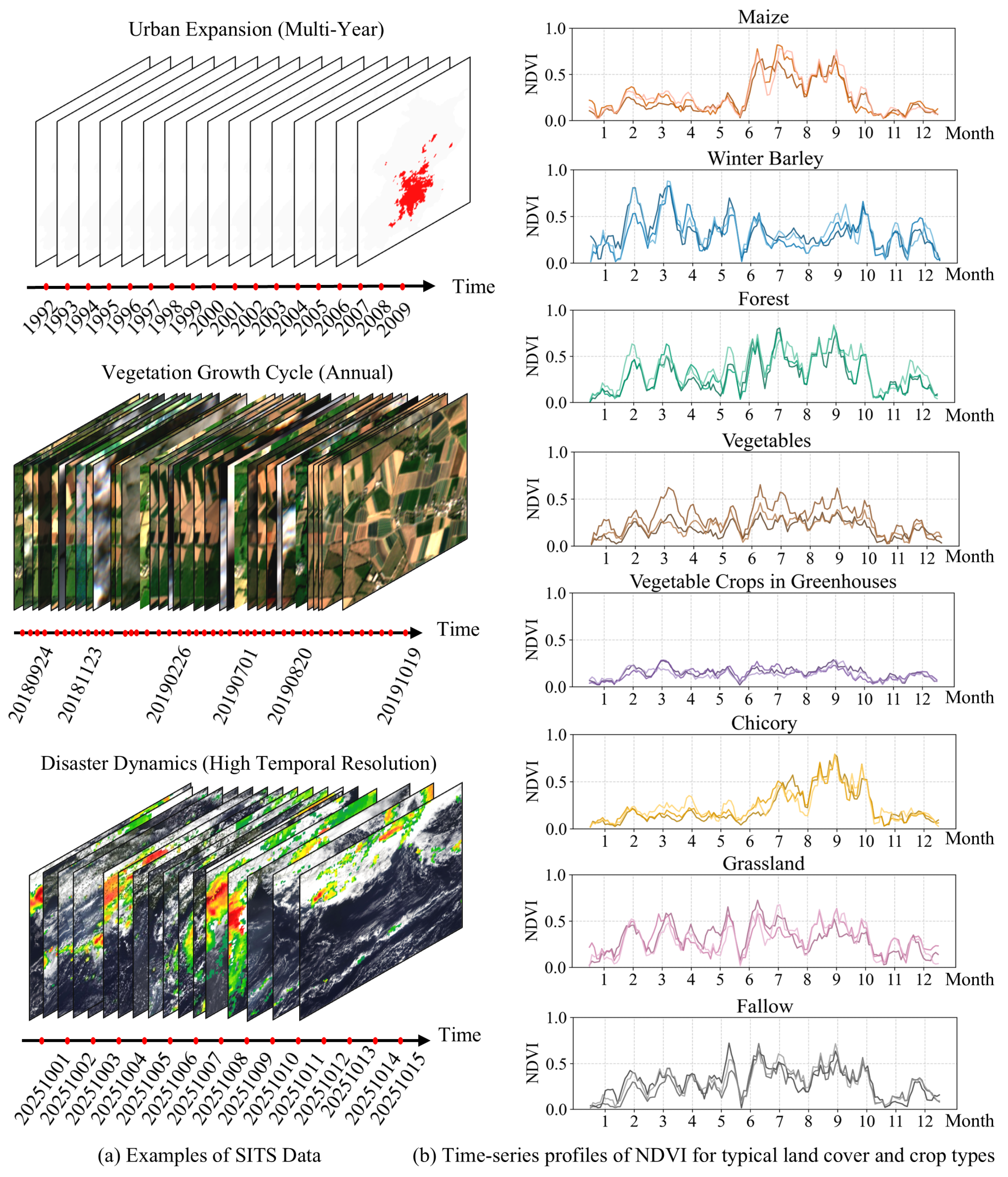
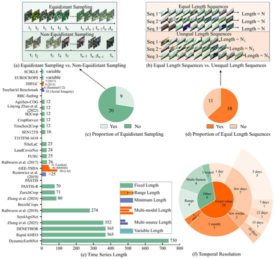
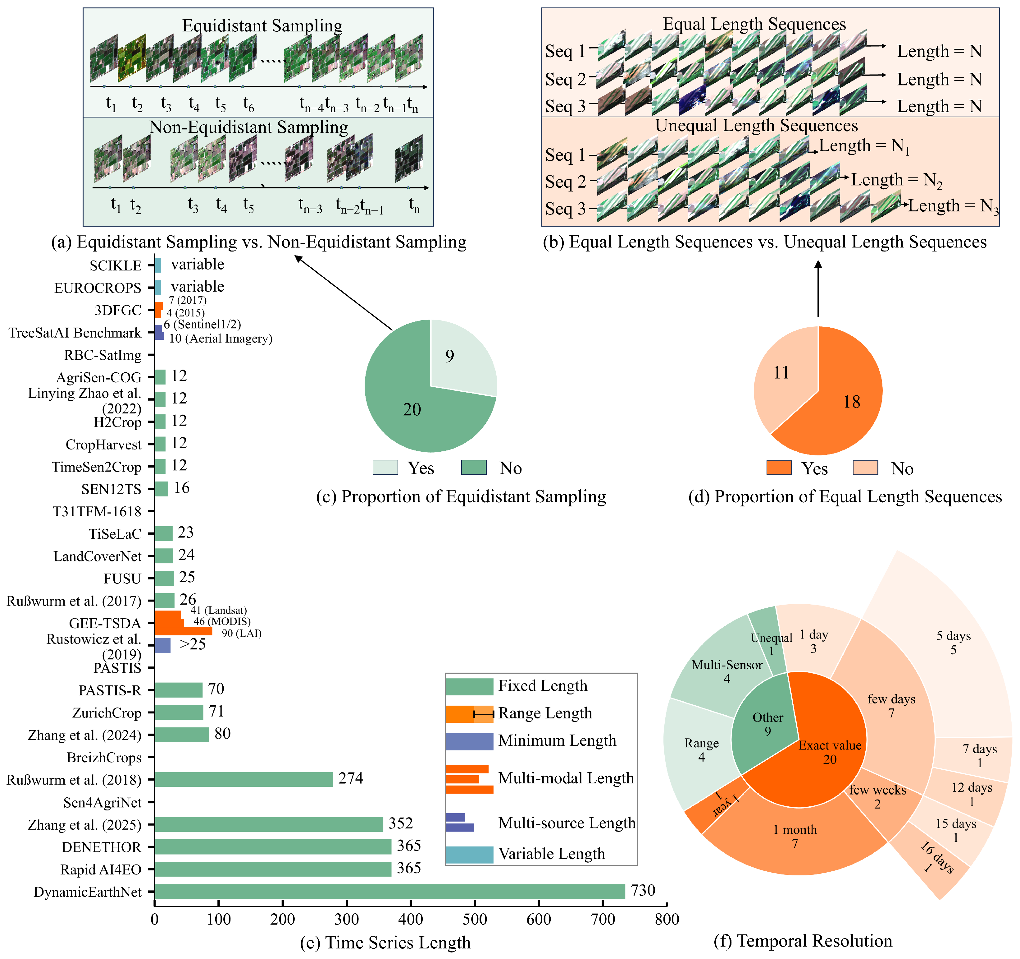
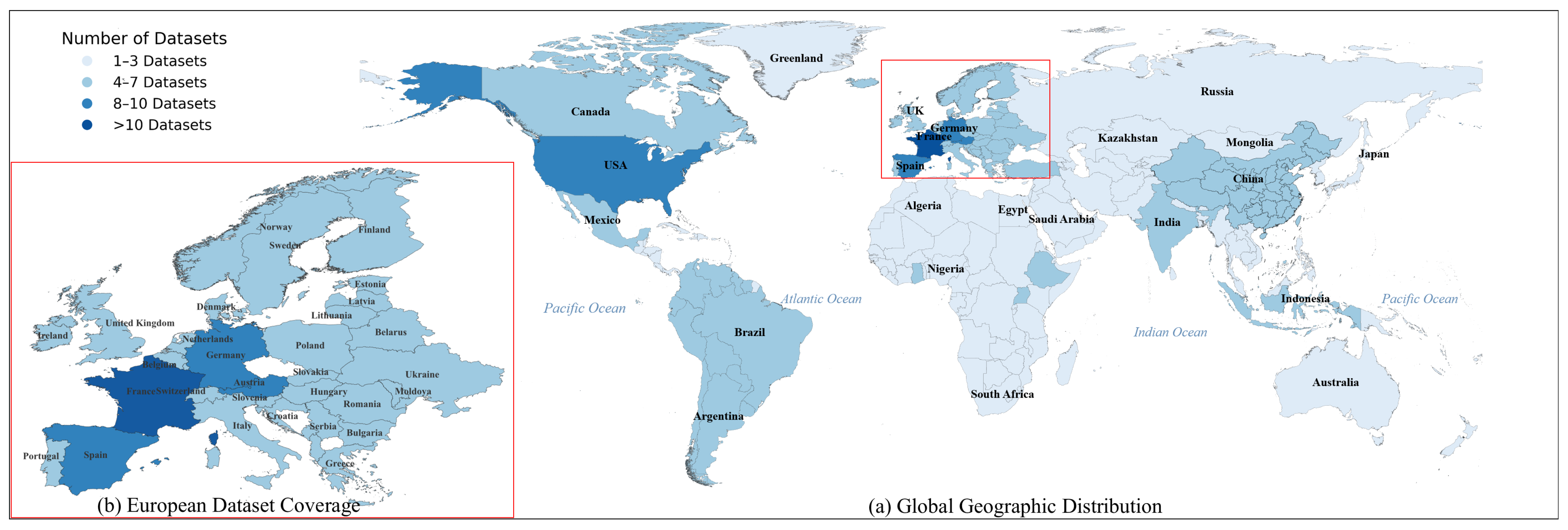
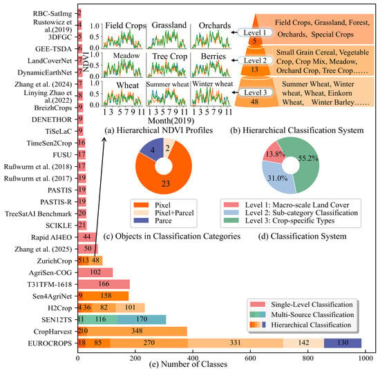
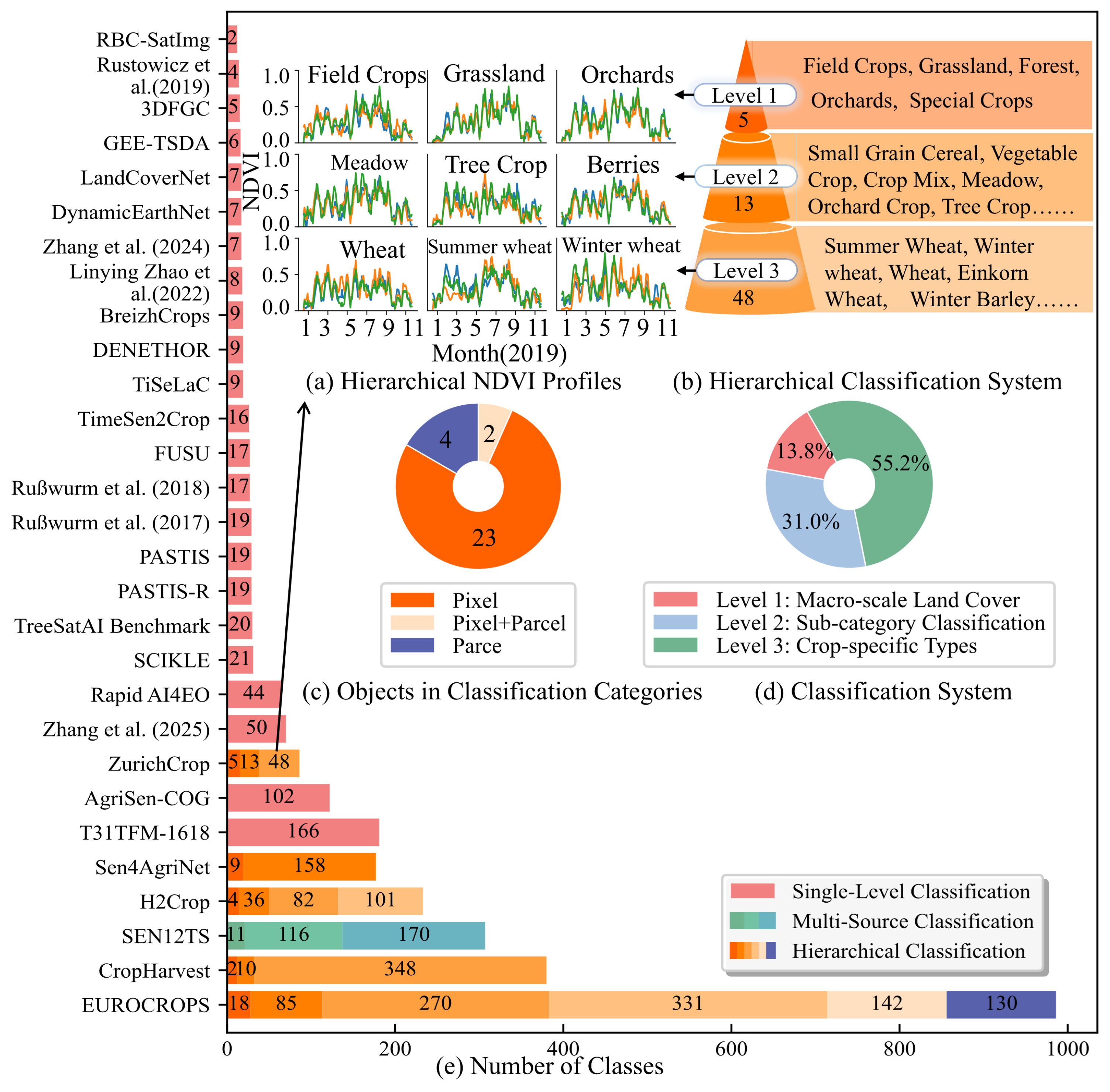
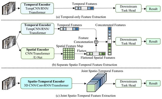
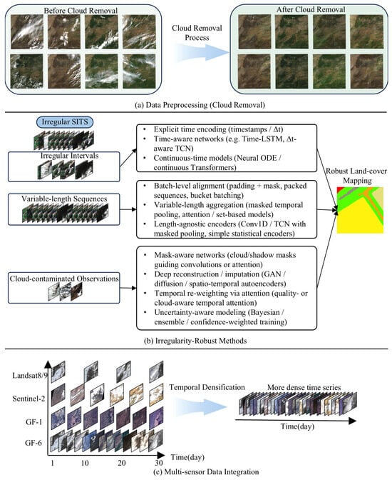
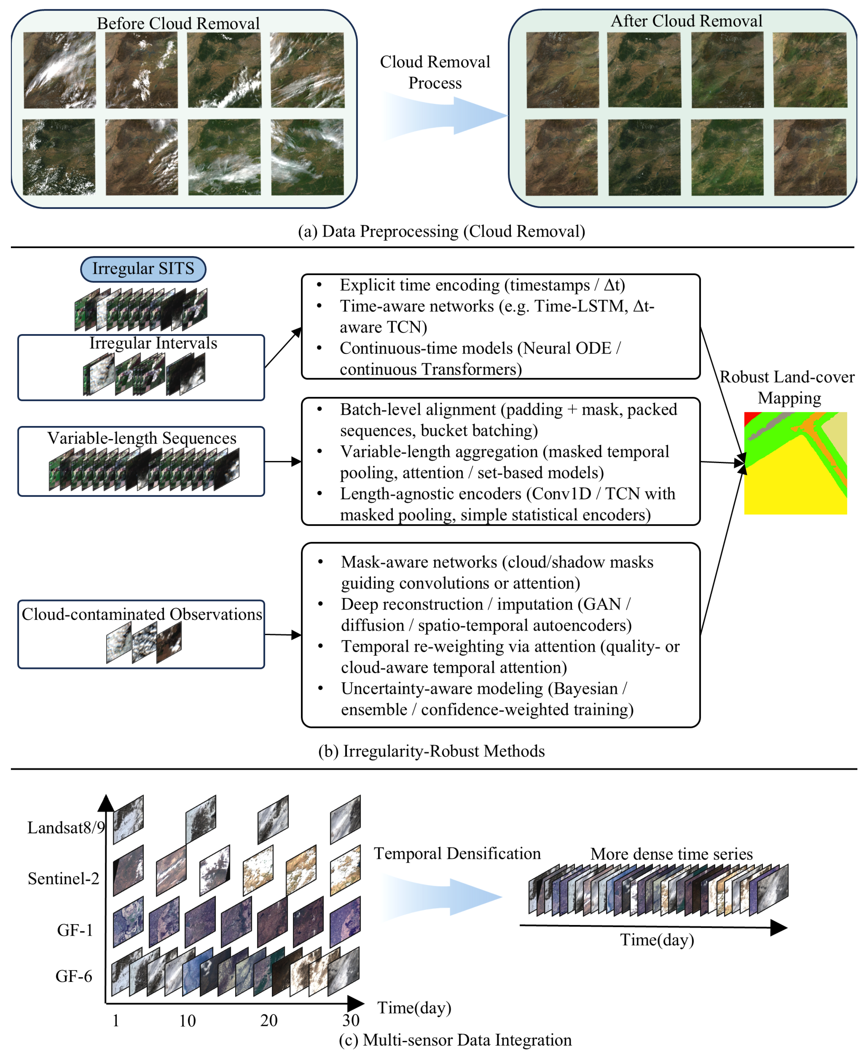
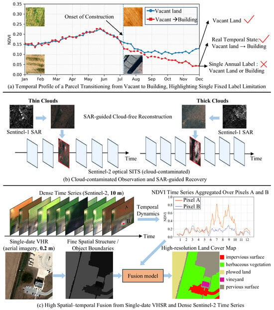
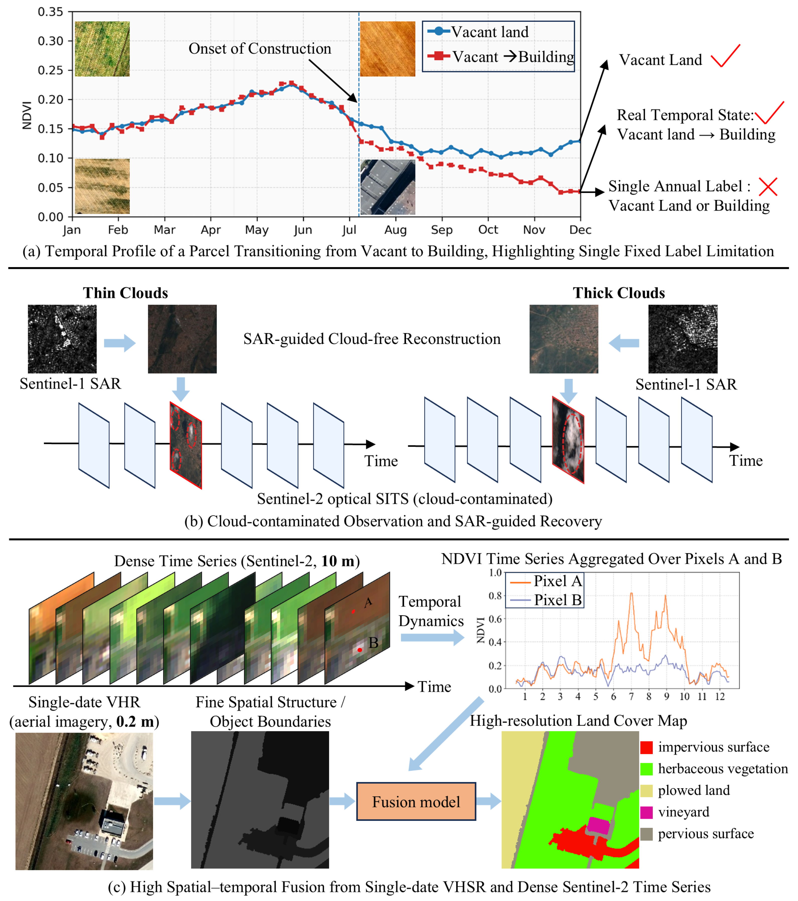

Disclaimer/Publisher’s Note: The statements, opinions and data contained in all publications are solely those of the individual author(s) and contributor(s) and not of MDPI and/or the editor(s). MDPI and/or the editor(s) disclaim responsibility for any injury to people or property resulting from any ideas, methods, instructions or products referred to in the content. |
© 2026 by the authors. Licensee MDPI, Basel, Switzerland. This article is an open access article distributed under the terms and conditions of the Creative Commons Attribution (CC BY) license.