Forest Disturbance Classification Under Imbalanced and Small-Sample Conditions Based on Collaborative Semi-Supervised Learning and Sample Generation

Highlights

What are the main findings?

• The proposed framework for multi-type forest disturbance classification based on collaborative semi-supervised learning and sample generation enables effective use of unlabeled data and suppresses pseudo-label noise. The method achieves robust classification under imbalanced and small-sample conditions, with an overall accuracy of 93.2%, outperforming single classification methods.
• The latent diffusion model effectively addresses class imbalance by generating high-fidelity pseudo-samples for rare disturbance types. The generated samples are consistent with real spectral and spatial patterns, improve class balance, and further enhance classification performance.

What are the implications of the main findings?

• The study provides a practical solution for forest disturbance classification when labeled samples are scarce and class distribution is highly imbalanced.
• Provides a practical and generalizable method for precision forestry; it could be extended to other remote sensing tasks with similar small sample and imbalance issues. The method has the potential to improve forest management, carbon accounting, and ecological assessment.

Abstract

Accurate and timely information on forest disturbance drivers is important for sustainable forest management, global carbon cycle accounting, and climate change response. However, forest disturbance classification is difficult due to two major challenges: limited labeled samples and highly imbalanced disturbance class distribution. In this article, a new framework for multi-type forest disturbance classification based on collaborative semi-supervised learning and sample generation was proposed. First, forest disturbance is detected using long-term remote sensing time series data and disturbance detection algorithms. Spatiotemporal, spectral and terrain features of different disturbance types are extracted. On this basis, to address the problem of imbalanced and small-sample conditions, a collaborative classification strategy is developed. Based on a small number of labeled samples, Support Vector Machine (SVM) and Random Forest (RF) are used to build dual base classifiers. A confident learning (CL) framework is applied to select high-confidence pseudo-labeled samples from unlabeled data. Then, a latent diffusion model (LDM) is introduced to generate high-fidelity pseudo-samples. This increases the sample size and balances the class distribution. Based on the augmented dataset, the dual classifiers are iteratively optimized using a co-training strategy, which improves model generalization under complex conditions. The results show that the proposed framework could generate high-quality pseudo-samples and effectively reduce class imbalance. The overall accuracy (OA) of the proposed framework reaches 93.2%, which is 5.7% and 4.4% higher than single classifier baselines, respectively. After introducing the LDM-based balancing mechanism, performance is further improved by 1.8% compared with the pure semi-supervised framework. This study provides an efficient and reliable solution for large-scale forest ecosystem monitoring.

1. Introduction

Forest ecosystems are a key component of the terrestrial system and play an important role in climate regulation, biodiversity conservation, and carbon sequestration [1,2,3]. However, forest disturbances driven by global climate anomalies, such as intensified wildfire regimes, together with human activities including logging, road construction, and land clearing, are placing serious pressure on the structure and function of forest ecosystems [4,5,6,7,8]. Accurate classification of forest disturbance types and their driving factors is important not only for understanding forest succession, but also for supporting ecological management decisions [9,10,11].

In recent decades, long-term satellite remote sensing data, such as the Landsat series, have provided new opportunities for detailed characterization of forest disturbance. The research focus has shifted from detecting whether disturbance occurs to classifying the type of disturbance [12,13,14,15]. Different driving factors lead to different spectral, structural, and functional responses, and these responses are complex and dynamic. Based on whether disturbance detection is performed before classification, methods for forest disturbance classification using remote sensing time series can be divided into direct methods [16] and two-stage methods [17]. The direct method uses temporal spectral metrics derived from remote sensing time series and prior knowledge of disturbance drivers to simultaneously detect and classify disturbance at the pixel level [18,19]. This method has higher efficiency because it does not require merging disturbance patches. However, the direct method is difficult to distinguish disturbance types with similar spectral features but different drivers without considering spatial context. It also tends to produce fragmented results with salt-and-pepper noise. One strategy in the two-stage method first detects disturbance at the pixel level using change-detection algorithms [20,21,22]. Then, disturbed pixels are grouped into patches, and spatial and spectral features of disturbance events are extracted [23]. Machine learning models or deep learning models are then used for classification. Another strategy is to use existing disturbance detection products, such as the global 30 m forest change dataset produced by the University of Maryland [24], and then classify disturbance types using machine learning algorithms [25,26]. The advantage of the two-stage method is that it operates at the patch level and can use more spatial information. Therefore, it is currently the main approach for forest disturbance classification [27,28]. For example, direct methods include change-vector analysis and within-year disturbance labeling using time-series spectral trajectories, while two-stage methods commonly combine LandTrendr, CCDC, COLD, or similar disturbance detection algorithms with subsequent machine-learning attribution.

Most existing methods require a large number of labeled samples to build classification models. Previous studies often collect samples through visual interpretation using historical records, high-resolution imagery, and field surveys [29,30]. For example, Li et al. collected 1708 disturbance patches using high-resolution images from Google Earth, including 632 wildfire samples, 345 logging samples, and 731 plantation samples [31]. However, high-quality labeled samples are expensive to obtain. In forest disturbance mapping, this difficulty is mainly caused by uncertain disturbance timing, cloud contamination, high field-survey cost, incomplete historical records, and the rarity of some disturbance types. In addition, disturbances such as road construction and fire are random and rare, which leads to a highly imbalanced distribution of disturbance types. To address the problem of imbalanced and small-sample conditions, current research mainly focuses on two directions. One is to develop methods for generating augmented labeled samples [32,33]. The other is to design methods that can achieve stable performance with limited labeled data [34,35].

Data augmentation methods aim to learn the latent evolution of disturbances in temporal, spatial, and spectral dimensions and generate high-quality pseudo-samples at scale [36]. By increasing the number of minority-class samples, these methods can correct class imbalance and provide important data support for improving classification accuracy. Previous methods, including basic transformations, mixed sample [37], can reduce data scarcity in the feature space, but they often ignore the physical consistency of spectral features and cannot represent spectral variability under complex land surface conditions. Generative Adversarial Networks (GANs) have been introduced into remote sensing to generate pseudo-samples [38]. However, conventional GAN-based methods may suffer from mode collapse when dealing with extremely small samples and may have difficulty capturing fine distributions in high-dimensional feature spaces. Generative models represented by latent diffusion models (LDMs) have shown strong ability in distribution modeling [39]. Compared with GANs, LDM is based on probabilistic generation. It can learn the statistical distribution of a small number of high-quality samples and generate disturbance features under different intensities and geographic conditions. This helps reduce feature sparsity caused by limited sampling. At the same time, LDM can reconstruct the distribution of rare classes and provide more representative and difficult samples. This improves model robustness under imbalanced small-sample conditions. Previous studies have shown that LDM can generate data with both diversity and high fidelity, which provides a new solution to the problem of sparse feature space in remote sensing [40,41].

When labeled samples are limited, existing methods mainly include transfer learning [42,43] and semi-supervised learning [44,45]. Transfer learning focuses on transferring feature-extraction ability from large public datasets to specific tasks, such as BigEarthNet [46]. However, datasets specifically designed for forest disturbance classification are very limited [47,48], so pretrained models cannot learn sufficient prior knowledge of disturbance patterns. In addition, differences in sensors, acquisition time, and geographic regions lead to domain differences, which often cause spectral mismatch in cross-region transfer. For disturbances with strong regional characteristics, such as specific logging patterns, the lack of targeted training data and limited generalization of transferred features restricts model performance. Semi-supervised learning uses large amounts of unlabeled data to compensate for the lack of labels. Typical methods, such as pseudo-labeling and consistency regularization, rely on model confidence to guide training. For example, Yan et al. used a confident learning (CL) framework to iteratively select high-confidence samples from unlabeled data and expand the labeled dataset [49]. However, this type of method is essentially a second selection from existing unlabeled data. Although it can increase sample size, its performance depends strongly on the quality of the initial labeled samples and the natural distribution of unlabeled data. Under extremely imbalanced conditions, CL often cannot obtain enough minority samples and may introduce label noise, which causes the classification boundary to shift toward majority classes. In addition, simple sample selection cannot reconstruct the feature distributions of rare classes and therefore cannot fundamentally solve the bias caused by class imbalance. To address this problem, the combination of LDM and CL frameworks can improve both data representation and model robustness through feature generation and knowledge alignment.

Based on these challenges, this study uses long-term remote sensing data to extract rich temporal, spectral, and spatial features of forest disturbance. A new framework is proposed by integrating LDM-based sample generation and the Mutual Guide Framework (MGF) for CL. Under the condition of limited and highly imbalanced labeled samples, this framework provides an efficient and reliable solution for large-scale and fine classification of forest disturbance in complex environments.

2. Study Area and Data

2.1. Study Area

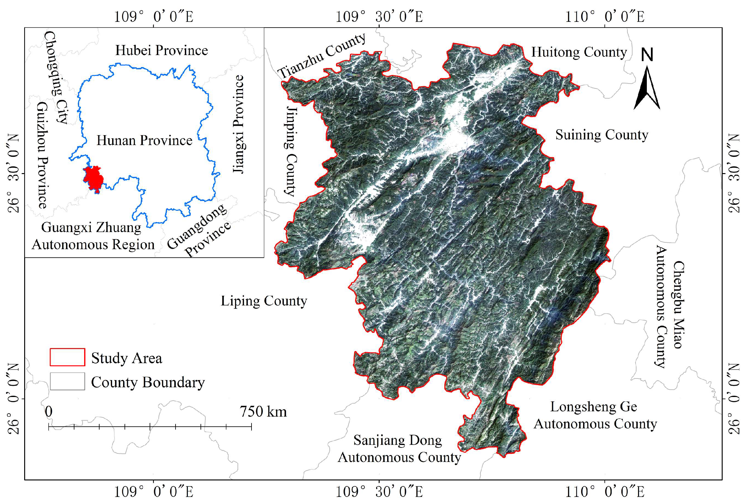
The study area is located in Jingzhou Miao Autonomous County and Tongdao Dong Autonomous County in the southern part of Huaihua City, Hunan Province, China (25°52′N to 26°47′N, 109°16′E to 110°01′E) (Figure 1). The forest coverage rates of Jingzhou and Tongdao are approximately 74.93% and 77.24%, respectively. The main forest type is the mid-subtropical humid evergreen broadleaf forest. This region belongs to karst topography. Due to the influence of special geological and soil conditions, extreme climate, as well as driving factors such as deforestation and mining, the forest ecosystem in this area is fragile and highly susceptible to disturbances, leading to degradation of the forest ecosystem. Therefore, this study selects four types of forest disturbances: road construction, logging, clearing for cultivation, and fires, as the research objects, which are highly representative.

2.2. Landsat Time Series Data

To obtain forest disturbance data, Landsat time series data from 1986 to 2022 were used, including Landsat 5 TM, Landsat 7 ETM+, and Landsat 8 OLI/TIRS. To maximize data availability under the climatic conditions of the study area, all available Landsat images with cloud cover less than 80% were collected. Fmask algorithm was used for cloud removal. After processing, a total of 357 images were obtained. Statistics on the number of images by month are shown in

Table 1. Number of all available images by month.

Month	January	February	March	April	May	June	July	August	September	October	November	December
Number of Images	28	24	19	21	28	14	28	35	39	34	47	37

.

2.3. Training and Validation Data

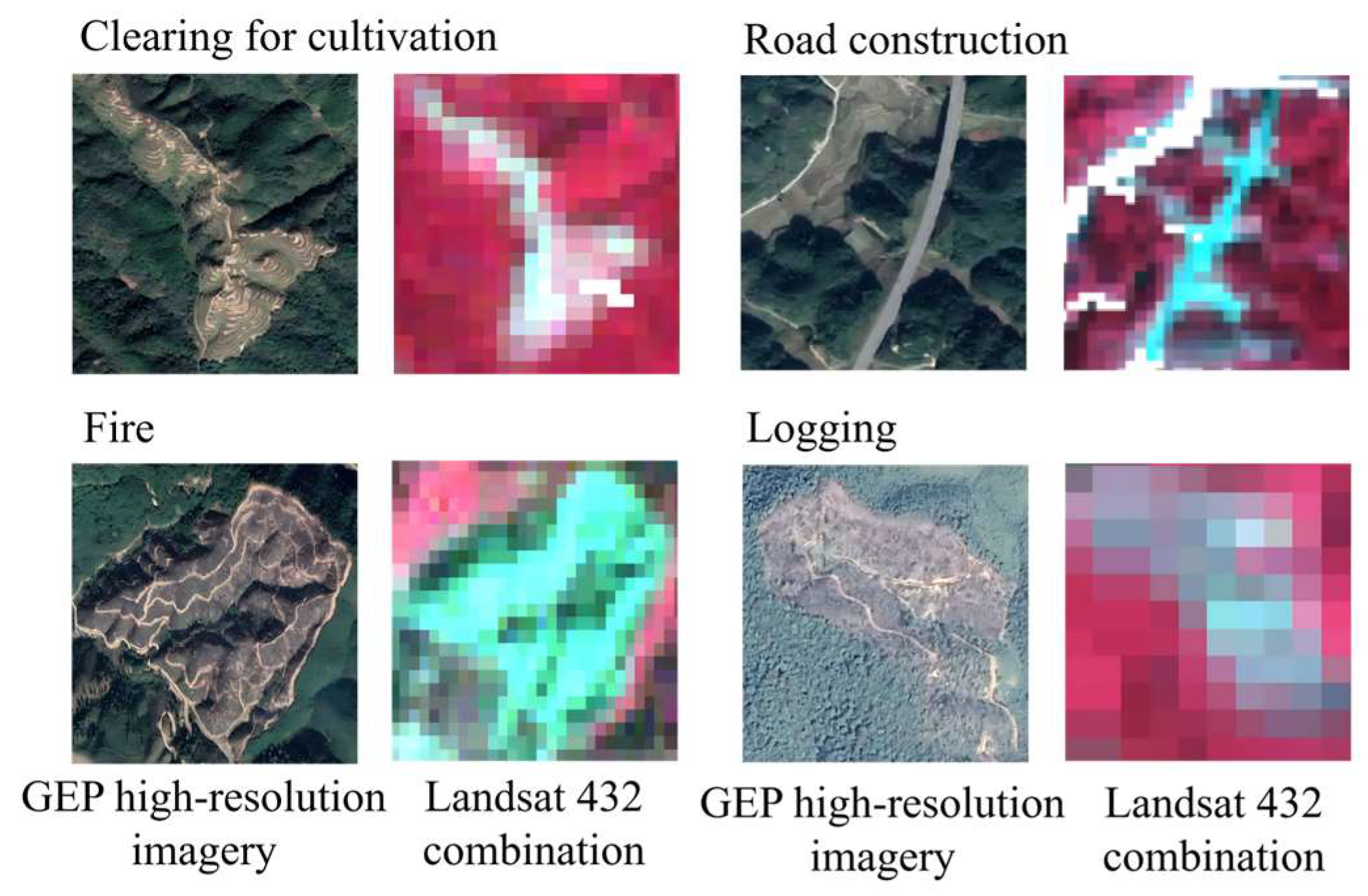
In this study, a forest disturbance sample dataset was constructed through multi-source data integration and visual interpretation. First, the Continuous Monitoring of Land Disturbance (COLD) algorithm was applied to preprocess Landsat series images. Harmonic model fitting and residual analysis were used to extract the spatial locations and occurrence time of potential disturbance patches. Disturbance samples derived from the COLD algorithm serve as baseline inputs for the subsequent collaborative semi-supervised learning and sample generation framework. Based on this, a forest disturbance dataset was built by integrating annual fire point data (obtained from the annual surface thermal anomaly dataset provided by the Institute of Remote Sensing and Digital Earth, Chinese Academy of Sciences), logging records (primarily collected from official government portals and news), and visual interpretation using Google Earth Pro (GEP, version 7.3.3). Figure 2 shows the true color and false color images for each type of disturbance. The disturbance types show a strong imbalance (

Table 2. Type and sample count of forest disturbance.

Disturbance Type	Description	Source	Sample Count
Road construction	Construction of roads and roadside service facilities within forests.	GEP	54
Logging	Forest disturbance caused by logging without conversion to other land-use types.	GEP and logging records	380
Clearing for cultivation	Clearing forests for crops or economic tree plantations.	GEP	86
Fire	Forest burning caused by fire, including wildfires and human-caused fires.	GEP and Landsat 8 annual fire hotspot data	142

).

The interpreted labels were cross-checked using temporal Landsat trajectories, available fire records, logging records, and GEP high-resolution imagery to ensure consistency between the disturbance type and the observed spectral-spatial evidence.

Among them, road construction and clearing for cultivation have very limited samples. The largest difference in sample size is about seven times. The dataset was split into training and testing sets with a ratio of 7:3.

3. Methodology

The framework of this study integrated multidimensional remote sensing features, semi-supervised learning, and sample generation methods for multi-type forest disturbance classification. First, long temporal Landsat images are used for forest disturbance detection and feature extraction. Then, a collaborative semi-supervised learning framework with a generative model is constructed. MGF is constructed using the heterogeneous properties of SVM and RF. To address the problem of sample limitation, CL is applied to identify label noise and select high-confidence pseudo-labeled samples from unlabeled data. A mutual guide strategy is used to iteratively refine the training dataset. In addition, to address the problem of sample imbalance, LDM is introduced for distribution reconstruction. This helps balance the feature space and improves classification performance.

3.1. Spatiotemporal and Spectral Response Analysis and Feature Construction of Forest Disturbance

The COLD algorithm is used for change detection in long-term Landsat data. The COLD algorithm fits seasonal patterns using a harmonic model and captures abrupt non-seasonal changes. This allows accurate detection of the timing and location of disturbances in complex forest environments. Based on the temporal trajectories for different disturbance types, a multi-dimensional feature space is constructed from temporal, spatial, spectral, and topographic aspects (

Table 3. Categorical features for forest disturbance attribution.

Type	Feature (Abbr.)	Spectrum Index (SI)	Description
Temporal features	Pre-change (PreC_SI), Post-change (PostC_SI), Change magnitude (MagC_SI)	NBR, SWIR1, TCW, TCG	Indices or band spectral values before and after change, and spectral differences between post-change and pre-change.
Spatial features	Pixel std in sliding window (STD_SI), Mean (Mean_SI)	NBR, SWIR1, TCW, TCG	Standard deviation and mean of indices or band values within sliding windows (3 × 3, 5 × 5, 7 × 7, 9 × 9).
Spatial features	Dissimilarity changes magnitude (MagDiss_SI), Contrast (MagCon_SI), Variance (MagVar_SI)	NBR, SWIR1, TCG	Differences in texture features (dissimilarity, contrast, variance) between post-change and pre-change (3 × 3 window).
Spectral features	Intercept change magnitude (Mag_INTP), Slope change magnitude (Mag_SLP)	INTP, SLP	Intercept or slope differences in the fitted segment trend line between post-change and pre-change
Terrain features	Elevation, Slope	DEM	Elevation and slope.

).

Temporal features include the pre-change spectral values (PreC_SI), post-change spectral values (PostC_SI), and change magnitude (MagC_SI = PostC_SI − PreC_SI). For spatial features, spectral mean (Mean_SI) and standard deviation (STD_SI) are calculated using sliding windows from 3 × 3 to 9 × 9. Texture differences before and after disturbance are also computed using a 3 × 3 window, including dissimilarity, contrast, and variance. To distinguish different disturbance types, spectral features are derived from differences between pre- and post-change temporal trajectories. These include the change in intercept (Mag_INTP) and slope (Mag_SLP). In addition, topographic features such as elevation and slope are included in the classification.

3.2. Forest Multi-Type Disturbance Classification Under Imbalanced Small-Sample Conditions Based on Collaborative Semi-Supervised Learning and Sample Generation

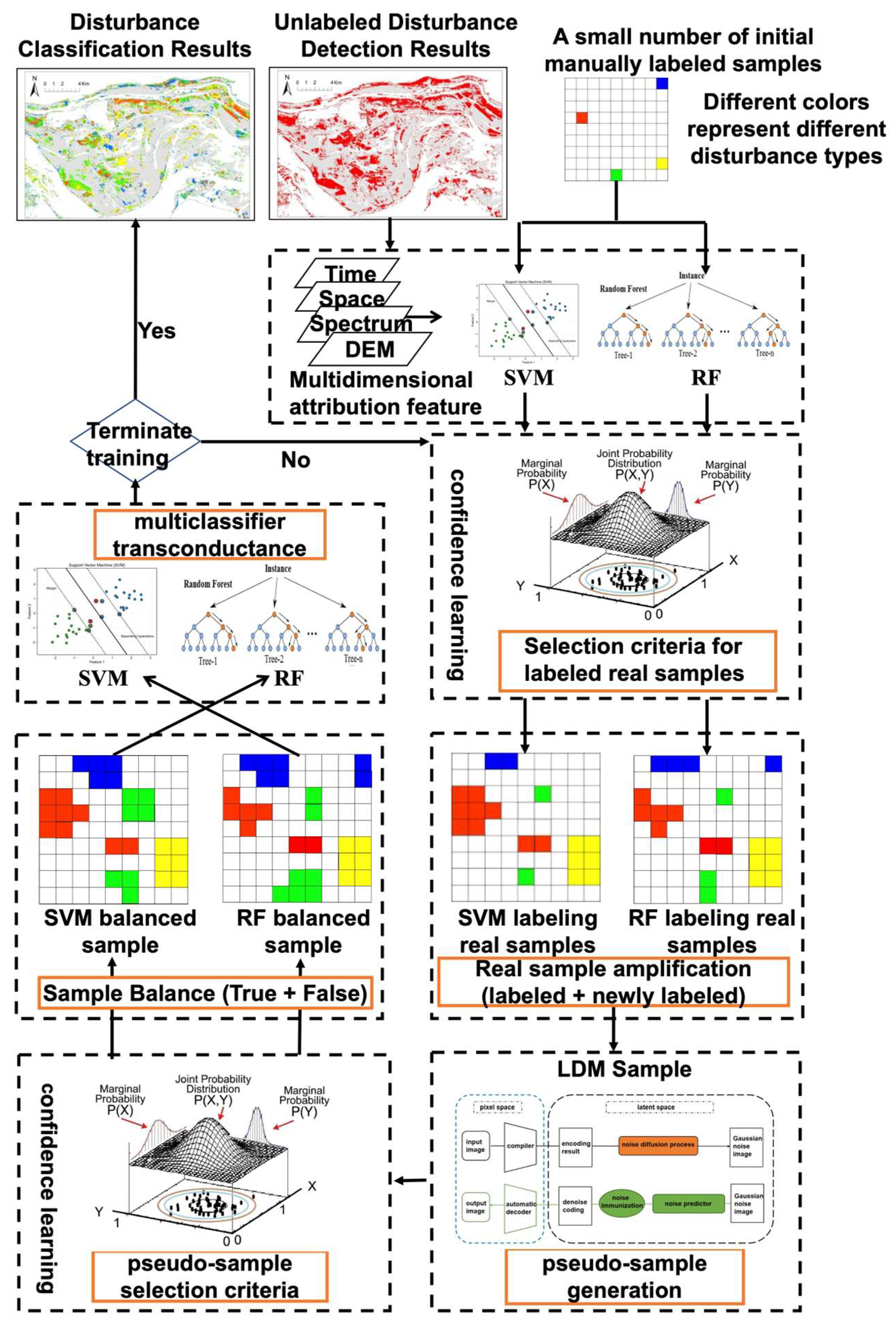
Based on the input multidimensional spatiotemporal, spectral, and terrain features, a Mutual Guide Framework (MGF) is constructed using SVM and RF as base classifiers to actively select high-confidence pseudo-labeled samples for expanding the ground-truth set. A sample generation method based on LDM is trained by utilizing the augmented labeled set from the MGF. Synthetic samples are generated to balance class proportions across different disturbance types. The MGF then re-trains its base classifiers using this balanced set to further identify pseudo-labeled samples. Throughout this process, a selection criterion based on Confident Learning (CL) is designed to specifically recruit high-confidence pseudo-labels and filter out low-quality generated samples. Through this cyclic iteration, a large-scale, highly reliable, and balanced labeled dataset is established, ultimately achieving high-precision forest disturbance classification under imbalanced small-sample conditions. The workflow is shown in Figure 3.

3.2.1. Forest Disturbance Classification Based on the MGF

The multi-dimensional features constructed in Section 3.1 are used as input for classification. To overcome the inductive bias of a single classifier under small-sample conditions, an MGF is built using two heterogeneous classifiers, SVM and RF. SVM and RF offer complementary learning mechanisms: SVM excels at finding global optimal hyperplanes with strong generalization under small-sample conditions, while RF captures local nonlinear relationships through ensemble decision trees. Their distinct global-versus-local perspectives provide the “multi-view” information necessary for CL, allowing the framework to identify noisy samples and suppress bias propagation through mutual guidance.

The workflow is as follows. First, the base classifiers are trained using a small set of labeled samples. They are then used to predict large-scale unlabeled disturbance data and assign initial pseudo-labels. To reduce noise in pseudo-labels, the CL criterion is applied to remove samples with ambiguous boundaries or inconsistent predictions. High-confidence pseudo-labeled samples are retained. A cross-guidance strategy is then used. High-confidence samples selected by classifier A are added to the training set of classifier B, and vice versa. The classifiers are retrained, and pseudo-label selection is repeated. Previously selected high-confidence pseudo-labeled samples are retained during later iterations and are not removed from the augmented labeled set. This process iteratively expands the labeled dataset and improves classification performance. After convergence, if the predictions of the two classifiers are consistent, the sample is assigned to that class. If not, the class with higher confidence is selected.

3.2.2. Pseudo-Sample Generation Using the LDM

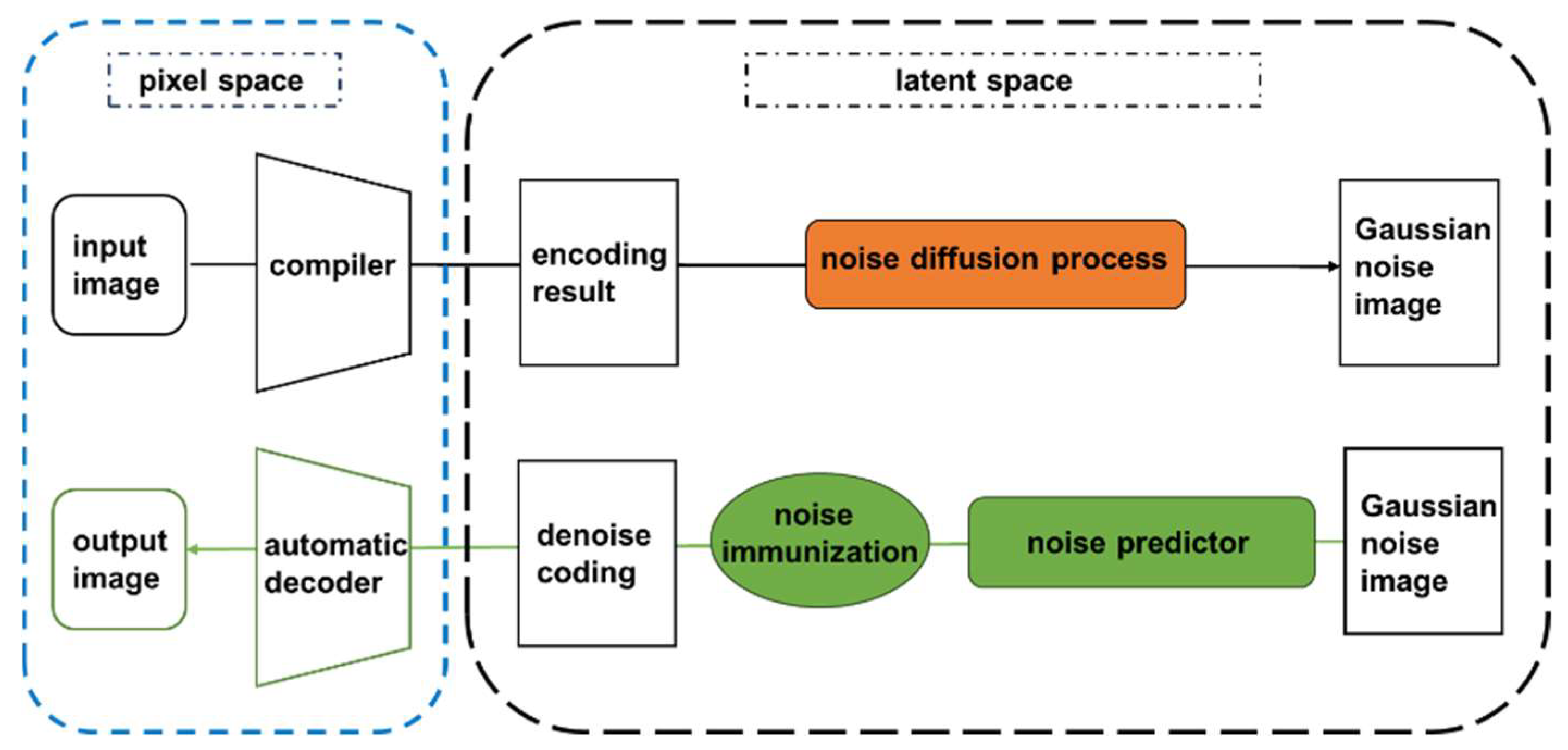
The LDM is used to learn the latent probability distribution of limited forest disturbance samples. It aims to generate high-fidelity pseudo-samples for minority classes. As shown in Figure 4, the framework includes two main levels: the pixel space and the latent space. The process consists of three key steps as follows.

The following description retains only the key LDM steps needed to explain forest disturbance feature generation.

Latent Space Mapping

To reduce computational cost in high-dimensional spatiotemporal and spectral feature space and suppress noise, a variational autoencoder (VAE) is used for latent mapping. An encoder $\epsilon$ maps the original disturbance feature vector $x$ into a low-dimensional latent representation $z=\epsilon \left(x\right)$. This step captures essential patterns of forest disturbance and succession. It allows the generation process to operate in a compact latent space.

Forward Diffusion and Conditional Denoising Learning

The LDM is based on two stochastic processes. In the forward diffusion process, small Gaussian noise is gradually added to the initial latent variable $z_0$ over $T$ time steps. This produces a sequence of noisy states $z_1,\dots , z_T$. When $T$ is large, the signal approaches isotropic Gaussian noise. The reverse process is a conditional denoising process and is used to generate pseudo-samples. A time-dependent denoising network ${ϵ}_{\theta }\left(z_t,t,y\right)$, based on U-Net, is trained to predict the injected noise. The model takes the noisy latent variable $z_t$, time step $t$, and disturbance class condition $y$ as input. The objective is to estimate the noise added at each step. The loss function is defined as follows:

$$L_{\left\{LDM\right\}}={\mathbb{E}}_{\left\{z, ϵ~\mathcal{N}\left(\mathrm{0,1}\right), t\right\}}\left[{‖ϵ-{ϵ}_{\theta }\left(z_t,t,y\right)‖}^2\right]$$

(1)

The guiding signal $y$ is derived from high-purity labeled samples filtered through confidence learning, ensuring the directionality of the generation process. This mechanism enables the precise synthesis of features corresponding to specific forest disturbance types based on practical requirements.

Reconstruction of Minority Class Pseudo-Samples

During the inference stage, the process originates from random Gaussian noise $z_T$. Guided by the target minority class label, the denoised latent vector ${\widehat{z}}_0$ is obtained through an iterative reverse denoising process. Finally, the VAE Decoder $\widehat{x}=D(^{\widehat{z}}_0)$ maps it back to the original multidimensional feature space.

The pseudo-samples synthesized via the LDM maintain high statistical consistency with the authentic samples. Moreover, they effectively capture the non-linear correlations between spectral bands under varying disturbance intensities. Compared to traditional interpolation-based augmentation methods, this generative probabilistic approach provides more diverse and physically meaningful hard examples. Consequently, it significantly enhances the decision robustness of the classifier when operating within highly imbalanced data environments.

3.2.3. Design of a CL-Based Criterion for Labeled Sample Augmented

To ensure the quality of augmented samples, this study incorporates the CL framework. By estimating the joint distribution between noisy labels and true labels, the framework enables the automated filtration of high-confidence samples.

The core of CL lies in estimating the joint distribution matrix $Q_{\tilde{y},y^{*}}$ through the correspondence between the sample’s predicted probability matrix and its noisy labels. The predicted probability $P\left(y=j|x_i\right)$ for sample $i$ belonging to class $j$ is obtained via cross-validation. For each class $j$, the average probability within the class assigned by the base classifier is calculated as the confidence threshold $t_j$:

$$t[j]={\displaystyle \frac{1}{\left|X_{\tilde{y}=j}\right|}}{\sum }_{x\in \tilde{y}=j}P(\tilde{y}=j,x,\theta )$$

(2)

where $\theta$ denotes the model. A counting matrix $C_{\tilde{y},\hspace{1em}{y}^{*}}$ (analogous to a confusion matrix) is then computed as follows:

$$C_{\tilde{y},\hspace{1em}{y}^{*}}\left[i\right]\left[j\right]:=\left|X_{\tilde{y}=i,y^{*}=j}\right|$$

(3)

where $X_{\tilde{y}=i,y^{*}=j}=\left\{xϵX_{\tilde{y}=i}:P\left(\tilde{y}=j,x,\theta \right)\ge t\left[j\right],j=\mathrm{a}\mathrm{r}\mathrm{g}\mathrm{m}\mathrm{a}\mathrm{x}P(\tilde{y}=l;\mathrm{x},\mathsf{\theta })\right\}$, and $l\in \left[m\right]$ satisfies $P(\tilde{y}=l;\mathrm{x},\mathsf{\theta })\ge t_l$.

Subsequently, the counting matrix is calibrated to ensure the total count matches the number of samples labeled by the base classifier:

$${\tilde{C}}_{\tilde{y}=i,\hspace{1em}{y}^{*}=j}={\displaystyle \frac{C_{\tilde{y}=i,\hspace{1em}{y}^{*}=j}}{{\sum }_{j\in \mathrm{1,2},3,\dots ,m}{C}_{\tilde{y}=i,\hspace{1em}{y}^{*}=j}}}\times \left|X_{\tilde{y}=j}\right|$$

(4)

where $\left|X_{\tilde{y}=j}\right|$ is the total number of samples with the pseudo-label $\tilde{y}=i$.

The joint distribution $Q_{\tilde{y},\hspace{1em}{y}^{*}}$ of noisy labels $\tilde{y}$ and true labels $y^{*}$ is estimated as follows:

$$Q_{\tilde{y}=i,\hspace{1em}{y}^{*}=j}={\displaystyle \frac{{\tilde{C}}_{\tilde{y}=i,\hspace{1em}{y}^{*}=j}}{{\sum }_{i\in 1,\dots ,m,j\in 1,\dots ,m}{\tilde{C}}_{\tilde{y}=i,\hspace{1em}{y}^{*}=j}}}$$

(5)

This joint distribution effectively reflects the distribution of noisy (erroneous) labels and true labels in real-world scenarios; as the data scale expands, this estimation increasingly converges toward the true distribution. Upon obtaining the joint distribution, a clean-up strategy is implemented for quality control based on the following criteria:

Consistency Filtering: Samples are identified where the class index corresponding to the maximum predicted probability does not match the label assigned by the base classifier. Samples falling into the non-diagonal units ($j\ne k$) of the counting matrix are filtered out as suspected noise.

Probability Gap Ranking: For samples in non-diagonal units, filtering is performed based on the estimated noise quantity $n_{jk}$ for each class. Samples with the smallest margin between the predicted probability and the threshold, calculated as $P\left(y=k|x\right)-P\left(y=j|x\right)$, are prioritized for exclusion.

3.3. Accuracy Evaluation Metrics

To quantitatively evaluate the similarity between the multidimensional pseudo-samples generated by the LDM and the authentic forest disturbance samples, the Fréchet Inception Distance (FID) is employed. Assuming that the feature distribution of the authentic samples follows a multivariate normal distribution with mean ${\mu }_r$ and covariance matrix ${\sigma }_r$, and the generated sample distribution follows a multivariate normal distribution with mean ${\mu }_g$ and covariance matrix ${\sigma }_g$, the FID is defined as follows:

$$FID\left({\mathbb{P}}_r,{\mathbb{P}}_g\right)=|{\mu }_r-{\mu }_g{|}_2^2+Tr\left({\Sigma }_r+{\Sigma }_g-2{\left({\Sigma }_r{\Sigma }_g\right)}^{1/2}\right)$$

(6)

where $Tr$ represents the trace of the matrix. A lower FID value indicates a higher degree of statistical similarity between the synthetic and authentic forest disturbance features, suggesting superior generative performance.

To quantitatively evaluate the fidelity of the physical attributes of the pseudo-samples, the Correlation Coefficient ($R$) is employed to measure the linear correlation between the synthesized and authentic spectral curves. The formula is as follows:

$$R={\displaystyle \frac{{\sum }_{i=1}^n\left(S_i-\overline{S}\right)\left(G_i-\overline{G}\right)}{\sqrt{{\sum }_{i=1}^n{\left(S_i-\overline{S}\right)}^2{\sum }_{i=1}^n{\left(G_i-\overline{G}\right)}^2}}}$$

(7)

where $n$ represents the total number of spectral bands in the Landsat imagery; $S_i$ and $G_i$ denote the mean spectral reflectance of the authentic and generated samples in the band $i$, respectively; $\overline{S}$ and $\overline{G}$ represent the overall average spectral reflectance across all bands. The value of $R$ ranges from [−1, 1].

The accuracy of both the disturbance detection and the classification models is assessed using a confusion matrix, which reflects the predictive performance for each individual category. Based on the confusion matrix, Overall Accuracy (OA), User’s Accuracy (UA)/Precision, Producer’s Accuracy (PA)/Recall, F1-score, and the Kappa coefficient are calculated.

The OA is calculated as follows:

$$OA={\displaystyle \frac{{\sum }_{i=1}^k{n}_{ii}}{N}}\times 100\%$$

(8)

where $k$ is the total number of classes, $n_{ii}$ represents the number of pixels correctly classified on the diagonal of the matrix, and $N$ is the total number of validation samples.

The PA is calculated as follows:

$$P{A}_i={\displaystyle \frac{n_{ii}}{n_{+i}}}\times 100\%$$

(9)

where $n_{+i}$ is the total number of reference samples for the disturbance class $i$. A higher PA indicates fewer omission errors for that specific category.

The UA is calculated as follows:

$$U{A}_i={\displaystyle \frac{n_{ii}}{n_{i+}}}\times 100\%$$

(10)

where $n_{i+}$ is the total number of pixels classified into the disturbance class $i$ in the classification map. A higher UA indicates fewer commission errors for that specific category.

$${F1}_i={\displaystyle \frac{2\times {Precision}_i\times {Recall}_i}{({Precision}_i+{Recall}_i)}}$$

(11)

The Kappa coefficient was used to evaluate the agreement between classification results and reference labels:

$$Kappa={\displaystyle \frac{(p_o-p_e)}{(1-p_e)}}$$

(12)

where $p_o$ is the observed agreement and $p_e$ is the expected agreement by chance.

4. Results

4.1. Evaluation of LDM Pseudo-Sample Generation Quality

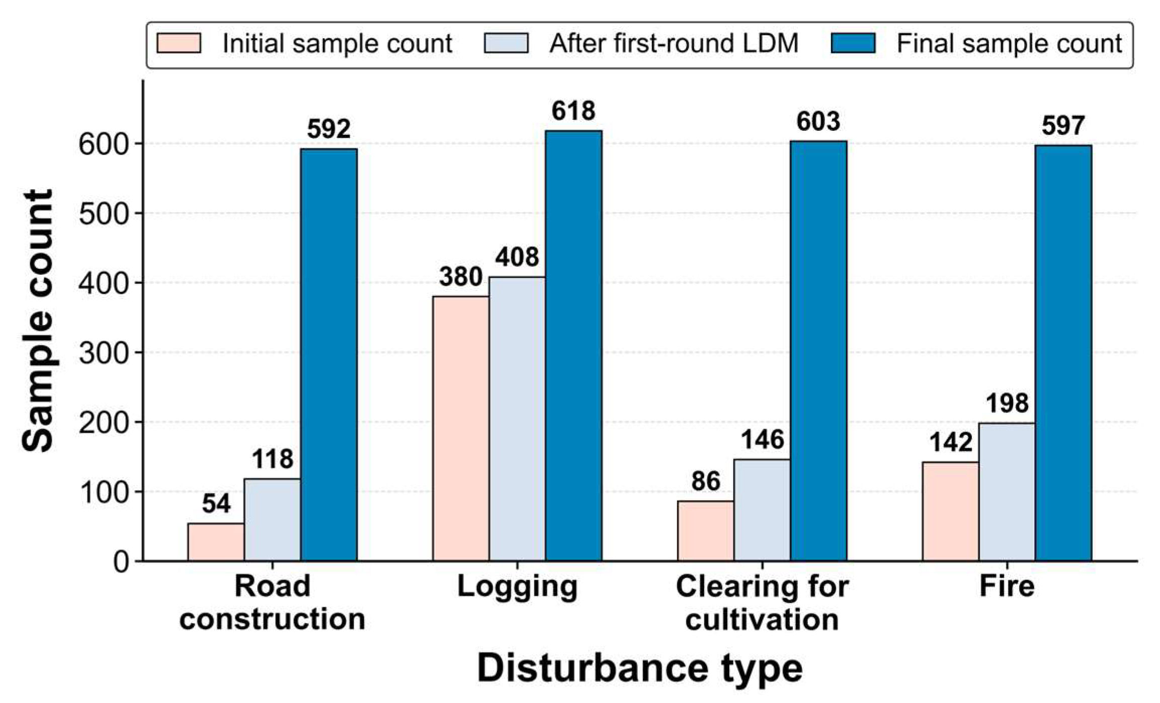
By introducing the LDM for targeted synthesis, the forest disturbance labeled sample database in the study area achieved a state of dynamic balance. In the original dataset, the ratio between majority and minority classes was as high as 7:1, exhibiting a typical long-tail distribution characteristic. In the initial stage, the LDM learned the underlying feature patterns of various disturbance types, leading to a steady increase in sample size across all categories through preliminary synthesis. Ultimately, through the synergy of class-specific guided generation by the LDM and semi-supervised sample augmentation within the SVM-RF framework, the scale of minority class samples was expanded to reach parity with the majority classes, while the total sample volume reached a sufficient level. As illustrated in Figure 5, the class frequency histogram transitioned from a prominent “step-like” structure to a stable, “levelled” distribution.

4.1.1. Qualitative Evaluation of Pseudo-Samples

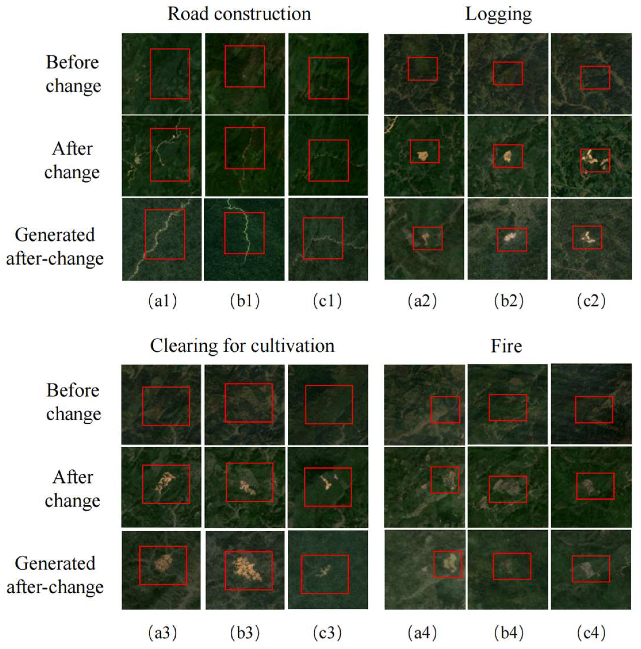
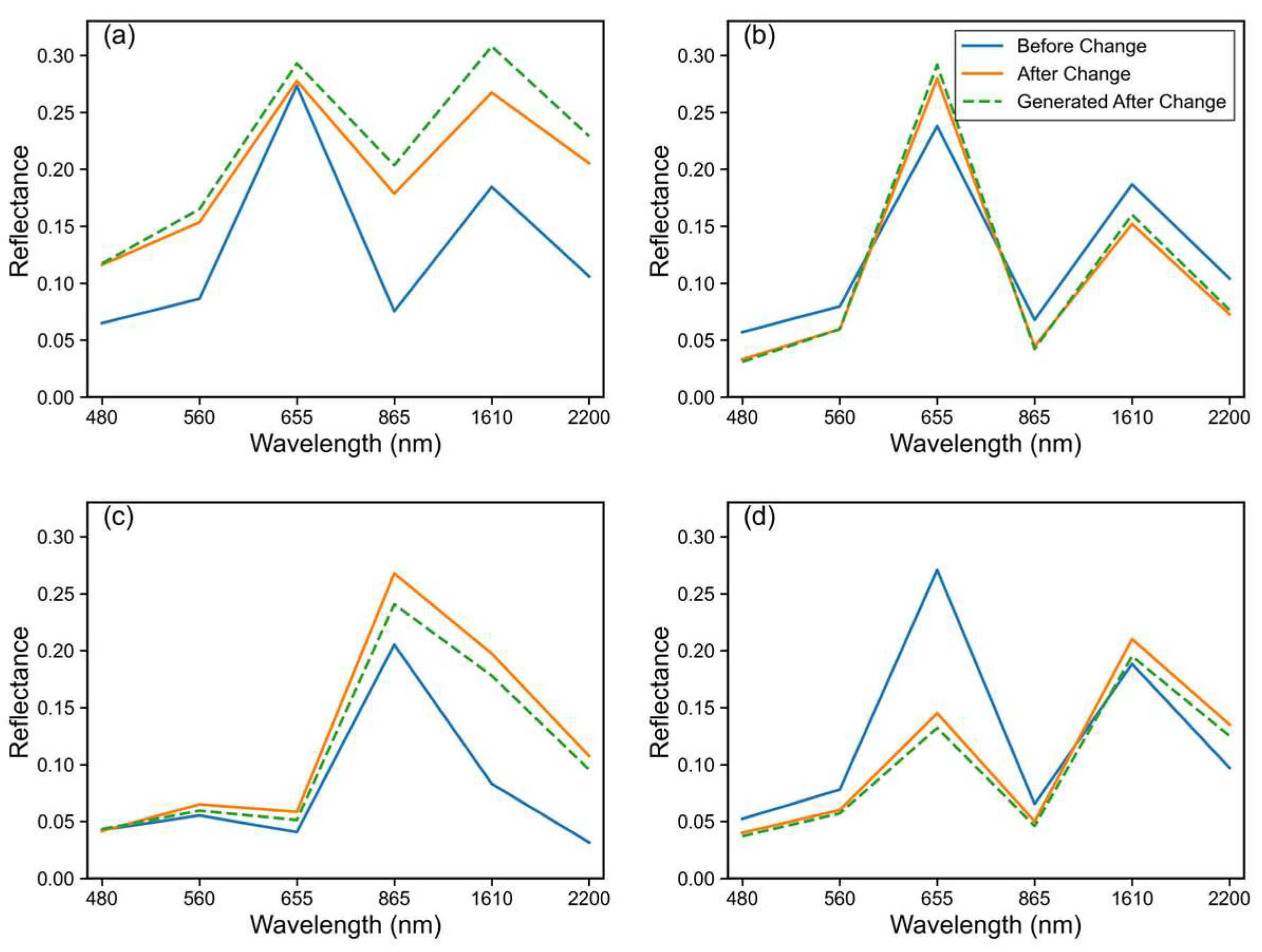
In this study, the physical fidelity of the generated data was qualitatively evaluated by comparing the visualization of authentic disturbance samples with LDM-generated samples before and after disturbances (Figure 6) and their corresponding spectral response curves (Figure 7).

As shown in Figure 6, the pseudo-samples generated by the LDM accurately replicate the spatial texture and color characteristics of authentic disturbance pixels across four disturbance types. Notably, in the Road Construction category, despite the extreme scarcity of initial labeled samples, the LDM successfully learned the dynamic evolution characteristics of artificial impervious surfaces (appearing gray-white) within complex forest backgrounds from the latent space. The generated post-disturbance images exhibit a high degree of similarity to authentic observations.

Regarding the morphology of spectral evolution, the pseudo-samples generated by the LDM precisely captured the spectral shift patterns driven by different disturbance factors. In the Road Construction class, a significant increase in reflectance across all bands was observed, particularly in the Short-Wave Infrared (SWIR, 1610 nm and 2200 nm) regions; the generated samples accurately reconstructed the high-reflectance properties caused by forest replacement with impervious surfaces or bare soil. In the Logging category, the synthesized samples successfully simulated the sharp decline in the Near-Infrared (NIR) band due to canopy loss, accompanied by a subtle increase in visible-light reflectance, reflecting the exposure of understory vegetation or soil. For the Clearance category, the LDM precisely captured the core shift pattern where reflectance in the Red (655 nm) and SWIR bands rises significantly during the initial clearing stage. In the Fire category, the carbonization of the land surface leads to a substantial decrease in reflectance across the entire spectrum. The curves generated by the LDM nearly overlap with the authentic ones, demonstrating exceptionally high fidelity in simulating the low-reflectance physical attributes of burn scars.

The high consistency in the spatiotemporal and spectral dimensions before and after changes forcefully demonstrates that the LDM could overcome the constraints of limited observation samples. By generating hard examples with rigorous spectral logic, the model provides high-quality data support for establishing robust classification decision boundaries.

4.1.2. Quantitative Evaluation of Pseudo-Samples

In this study, the FID and the $R$ were employed to quantitatively evaluate the quality of LDM-generated samples from two dimensions: feature space distribution and physical spectral fidelity (

Table 4. Quantitative evaluation results of pseudo-samples.

Disturbance Type	Original Count	FID	R
Logging	380	22.41	0.85
Fire	142	24.73	0.82
Clearing for cultivation	86	27.56	0.79
Road construction	54	29.18	0.76

). The results indicate that the LDM maintained consistently low FID values, even for disturbance categories with limited initial samples, such as road construction and clearing for cultivation. This suggests that the model has successfully captured the underlying manifold structure of minority class disturbances within the latent space, rather than performing simple pixel-level cloning. Such low FID values ensure that the augmented sample database not only achieves numerical balance but also accurately reflects the stochasticity and complexity of natural forest disturbances in terms of statistical characteristics. Furthermore, the correlation coefficients between the average spectral curves of authentic and generated samples demonstrate a high degree of consistency across the four primary forest disturbance types.

The synergistic performance of FID and the correlation coefficient proves that the LDM does not merely replicate samples. Instead, by learning the distribution patterns of minority disturbances, it achieves high-quality distribution completion. This provides a robust data foundation for mitigating the classification bias typically induced by sample imbalance.

4.2. Classification Accuracy Evaluation of Forest Disturbance Types

4.2.1. Overall Classification Accuracy Assessment

The proposed cross-guidance framework serves as the final tool for evaluating the classification accuracy of forest disturbance types. As presented in

Table 5. Confusion matrix for forest disturbance type classification based on confidence learning mutual guidance framework.

	Road Construction (Pred.)	Logging (Pred.)	Clearing for Cultivation (Pred.)	Fire (Pred.)	PA/Recall (%)	F1-Score (%)
Road Construction (Ref.)	50	3	1	0	92.6	92.6
Logging (Ref.)	3	353	9	15	92.9	94.8
Clearing for Cultivation (Ref.)	1	3	81	1	94.2	90.0
Fire (Ref.)	0	6	3	133	93.7	91.4
UA/Precision (%)	92.6	96.7	86.2	89.3	—	—
OA (%)	93.2					—
Kappa (%)	88.9					—

, the framework demonstrates exceptional performance in identifying the four forest disturbance categories, achieving an OA of 93.2%. The Recall values for all disturbance types exceeded 90%, while the Precision values for Clearing for Cultivation and Fire were relatively lower, at 86.2% and 89.3%, respectively. These results validate the robustness of the synergistic mechanism between generative augmentation and semi-supervised learning when addressing tasks characterized by imbalanced and small-sample datasets.

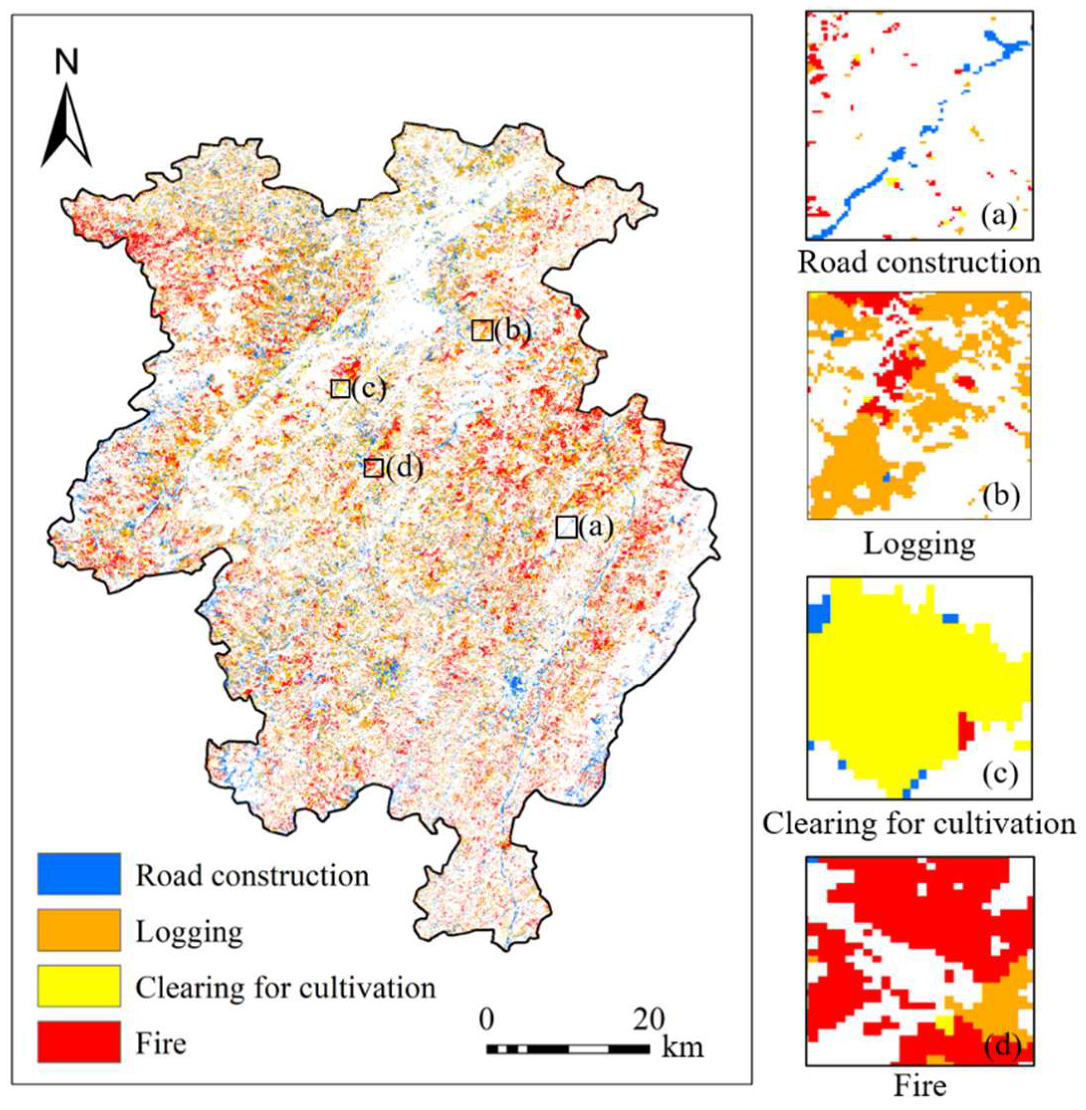
The annual spatial distribution of disturbance types from 2000 to 2021 is illustrated in Figure 8. Logging and Fire are the predominant disturbance types. Road Construction events are mainly distributed within the forest margins and peripheral regions. Four types of disturbances span nearly the entire study area. Based on the statistical analysis, the total forest area affected by various disturbance types reached 1392.3 km².

4.2.2. Ablation Experiment

To evaluate the effectiveness of the LDM and the MGF based on CL, four sets of ablation experiments were conducted (

Table 6. The results of the ablation experiment.

Strategy Number	Experimental Description	OA (%)	95%CI	p-Value vs. M4	Effect Size (Cohen’s d) vs. M4
M1	Original imbalanced small sample + Single RF classifier	87.5 ± 1.5	[86.4, 88.6]	<0.001	4.39
M2	Original imbalanced small sample + Single SVM classifier	88.8 ± 1.3	[87.9, 89.7]	<0.001	3.70
M3	Original imbalanced small sample + SVM-RF MGF based on CL	91.4 ± 1.0	[90.7, 92.1]	0.004	1.99
M4	LDM sample balancing + SVM-RF MGF based on CL	93.2 ± 0.8	[92.6, 93.8]	Reference	Reference

Note: OA values are reported as mean ± standard deviation based on 10 repeated random experiments. The p-values were calculated using paired t-tests by comparing each baseline strategy with M4. Cohen’s d was used to quantify the effect size of the improvement.

). By comparing classification performance across different strategies, the contribution of each module to addressing the imbalance in small sample sizes was analyzed.

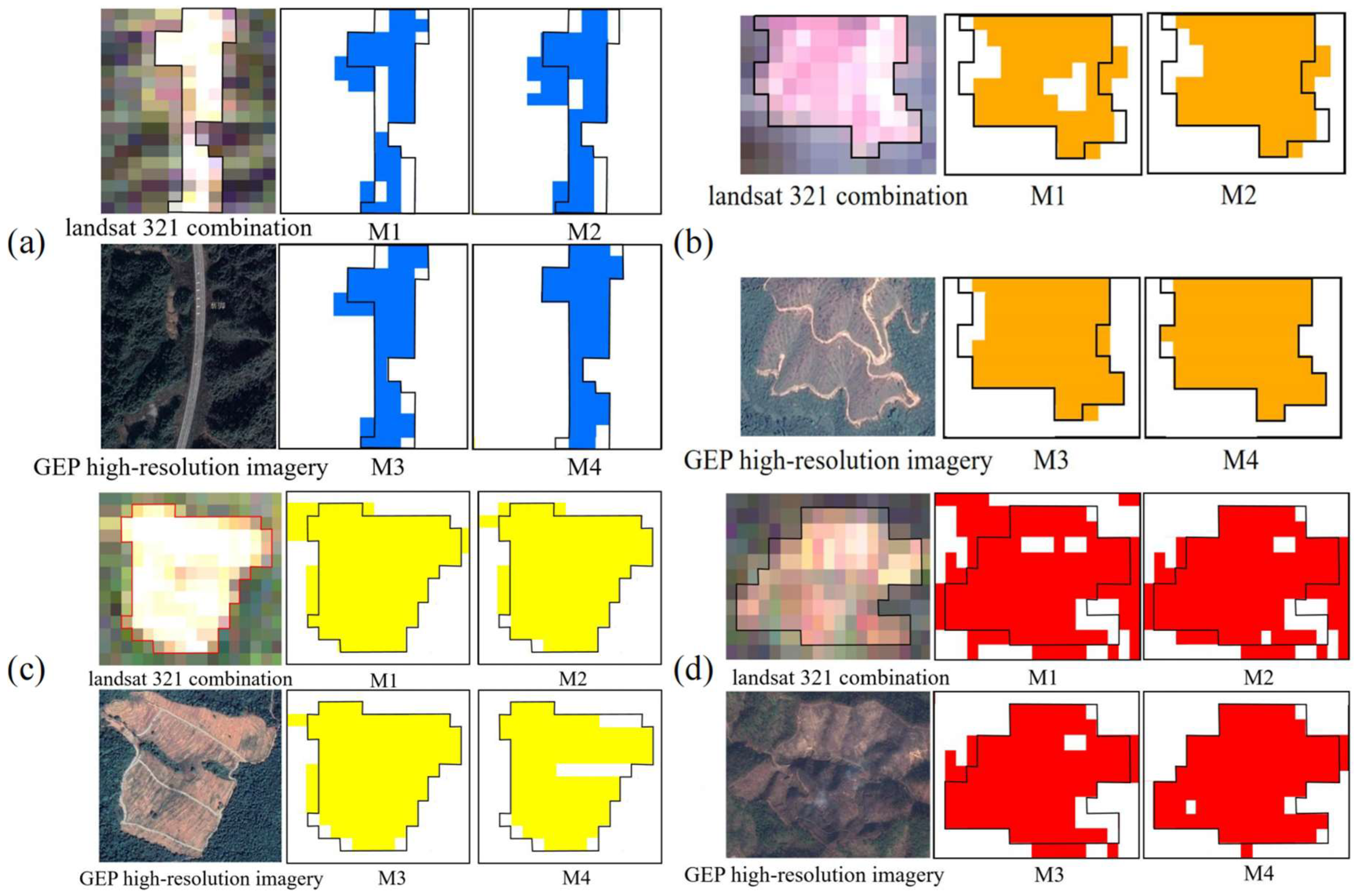
Due to the constraints of the original imbalanced and small-scale datasets, traditional single classifiers (M1 and M2) exhibited limited performance, with OA of 87.5% and 88.8%, respectively. Analysis of Figure 9 reveals a severe majority-class bias in the baseline models, driven by the sparsity of minority-class samples (e.g., Road Construction, Fire). This bias led to numerous fine disturbance patches being misclassified as background forest or large-scale logging areas. With the introduction of the MGF based on CL (M3), the overall accuracy improved to 91.4%. This demonstrates that the co-training mechanism can effectively extract high-confidence information from unlabeled data. However, M3 remained constrained by the long-tail distribution of the original data, and the improvement for extreme minority classes encountered a performance bottleneck (e.g., Road Construction). The complete framework proposed in this study (M4) achieved the highest classification accuracy, representing a further improvement of 1.8% over M3. The experimental results indicate that filtering at the algorithmic level alone is insufficient; distribution reconstruction via LDM at the data level is essential. As shown in Figure 9, a comparison between M3 and M4 reveals that M4 significantly reduces the omission rate for Road Construction. Significantly, in the clearing-for-cultivation sample, M4 effectively detected the long and narrow unchanged areas.

The powerful synergistic effect between the balanced distribution provided by the LDM and the high-quality filtration provided by CL not only completes the feature space of rare disturbances but also enhances the model’s discriminative robustness within complex landscape backgrounds.

To further evaluate the robustness of the ablation results, each strategy was repeated under different random seeds. The OA was reported as mean ± standard deviation, and statistical significance was assessed using p-values, Cohen’s d, and 95% confidence intervals.

The complete framework M4 achieved the highest mean OA and showed statistically significant improvements over the baseline strategies, indicating that the performance gain was stable across repeated experiments.

4.3. Error Analysis of Forest Disturbance Classification

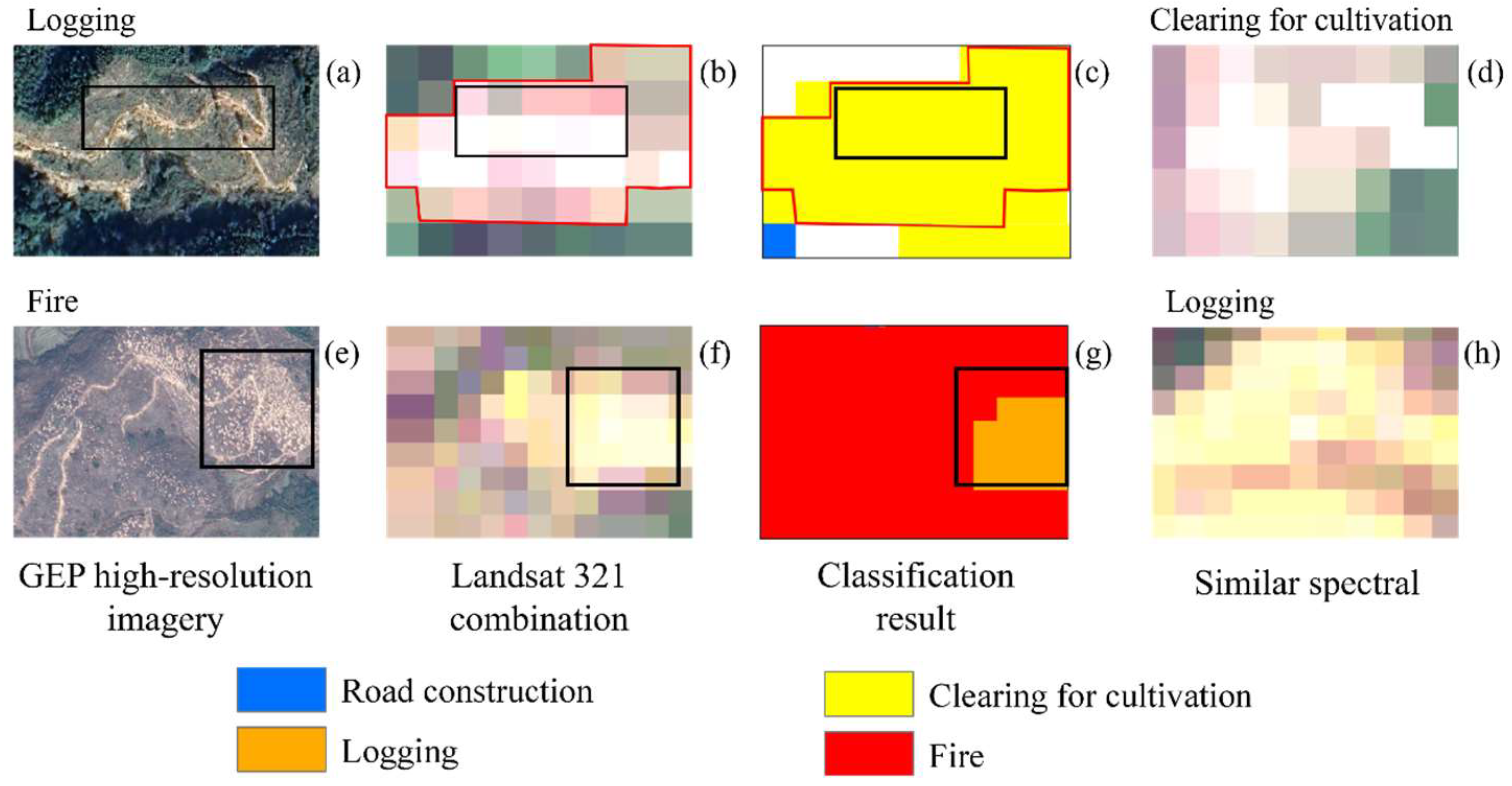
Figure 10 illustrates two typical cases of misclassification. In the region shown in Figure 10a–d, severe logging-induced canopy destruction resulted in extensive bare-soil exposure, exhibiting a characteristic gray-white tone. This appearance is highly similar to typical clearance features, leading to some logging areas being misclassified as clearing for cultivation. Under the constraints of extremely small sample sizes, the MGF relies heavily on the feature manifold of the latent space. Consequently, when the post-disturbance surface of a logging area exhibits such extreme atypical features, the model tends to categorize it into the clearance class due to their similar spectral responses. Also, this confusion may be attributed to the 30 m spatial resolution of Landsat images, because exposed soil, residual vegetation, and small disturbance boundaries can be mixed within one pixel.

Figure 10e–h present another representative misclassification case. In this region, the overall background is dominated by large-scale forest fire disturbances; however, a localized patch was incorrectly identified as Logging. This error occurred because the specific patch exhibited more thorough vegetation destruction compared to the surrounding fire-affected areas. The near-complete combustion of vegetation and organic litter layers led to high soil exposure, creating a high degree of physical similarity to commercial logging sites—specifically, forest clearing areas or temporary log landings. Although the MGF learned the typical spectral manifold of fires via the LDM, it remains susceptible to the spectral confusion effect when encountering “bright outlier” samples that deviate from the normal fire distribution due to extreme combustion. In such cases, the model defaults to the logging category, which offers a more consistent spectral match. This result indicates that fire scars under extreme combustion and logging sites with strong soil exposure may show similar mixed-pixel spectral responses at Landsat resolution.

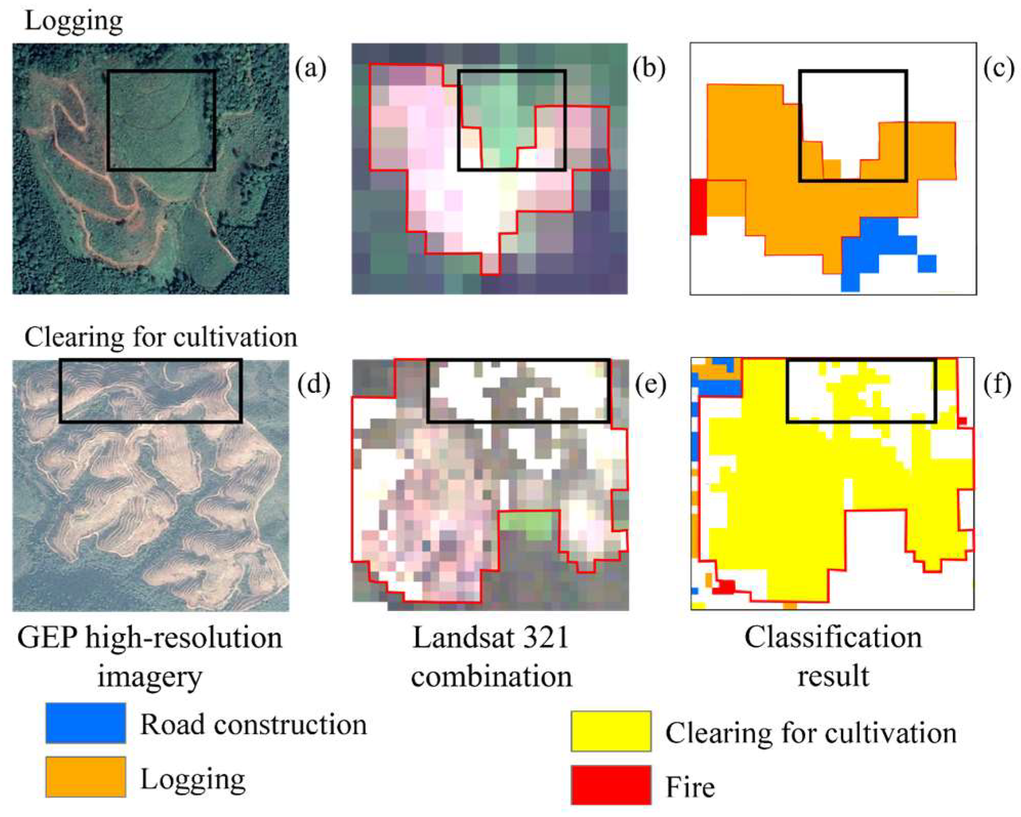
Figure 11 illustrates two representative cases of omission errors. In the region shown in Figure 11a–c, several logged patches are classified as undisturbed forest. Although these areas underwent logging, the ground surface was not entirely denuded; instead, it was rapidly covered by dense secondary herbaceous vegetation or residual understory. In the Landsat band 3-2-1 composite (false-color), these patches exhibit a prominent green hue, resulting in minimal spectral differentiation from healthy forest canopies. This rapid revegetation phenomenon (e.g., fast weed encroachment following selective logging) effectively masks the distinctive spectral signature of the underlying soil layer. Consequently, the model categorizes these pixels as stable forest, leading to significant omission.

In the region depicted in Figure 11d–f, certain clearing for cultivation areas were omitted due to the influence of cloud cover. During the data preprocessing stage, affected pixels were removed, preventing the MGF from acquiring the continuous feature evolution of these specific locations. The lack of temporal consistency in the spectral trajectory resulted in the failure to detect these disturbance events.

5. Discussion

The proposed framework effectively addresses the problems of small samples and class imbalance in forest disturbance classification. Although good classification performance is achieved, there is still room for improvement.

First, although the LDM shows strong performance and effectively alleviates class imbalance, it has high model complexity and requires substantial computational resources. Its advantage is not limited to the final OA improvement; it also provides minority-class distribution completion and reduces the bias caused by long-tailed samples. The diffusion model used in this study achieves high-quality sample generation but imposes high demands on computation and inference efficiency. This limits its deployment in resource-constrained environments. For forest disturbance monitoring at national or global scales, spatial transfer of model weights and incremental learning remain key challenges. Future work can explore lightweight diffusion models by integrating techniques such as knowledge distillation, model pruning, and structural reparameterization. This may enable efficient and low-power sample generation and improve the practicality and scalability of the framework across edge devices and large-scale systems.

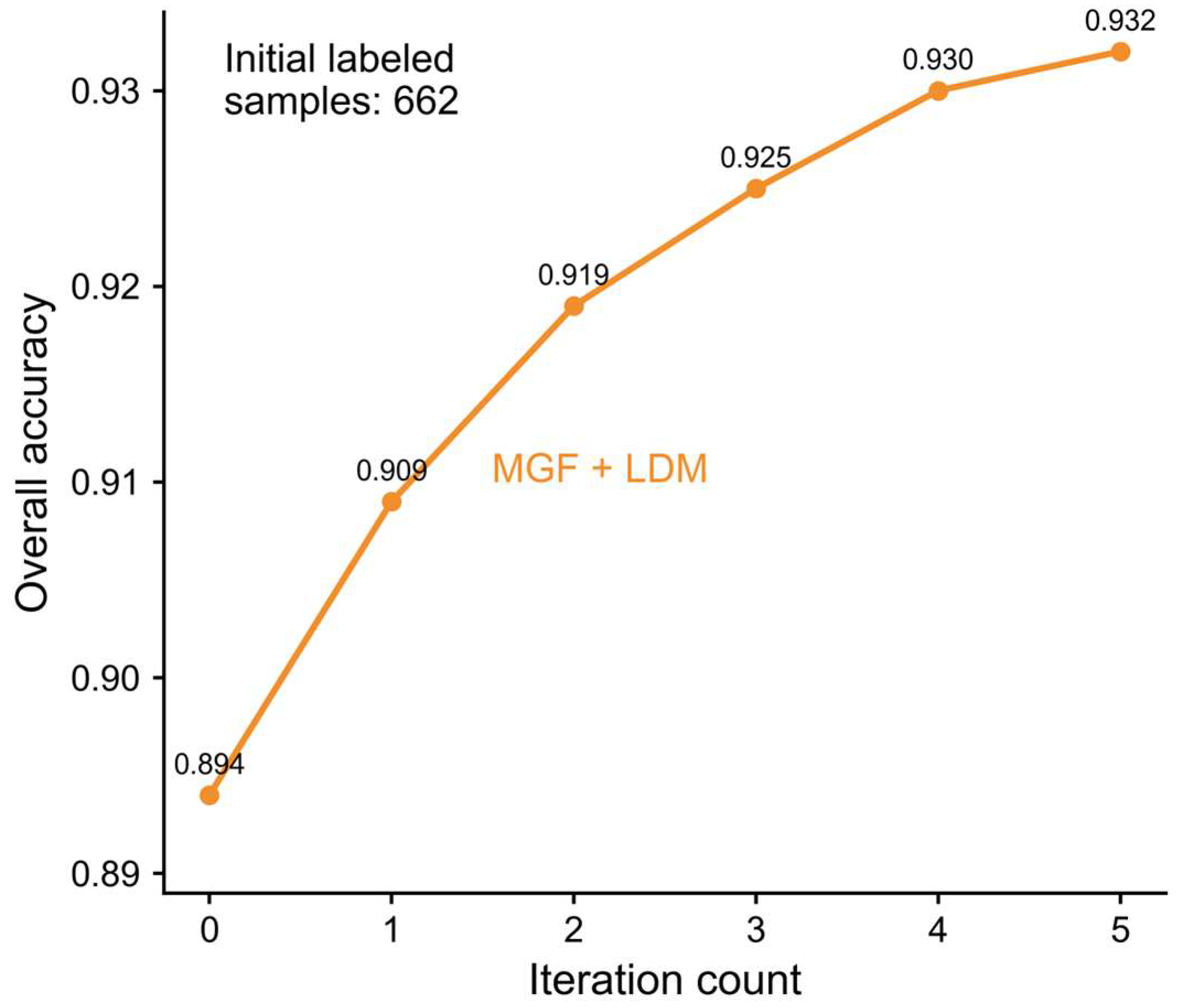
The requirement for data augmentation also has a learning-curve limitation. Increasing the number of generated samples can improve minority-class representation, but the improvement is not unlimited. As shown in Figure 12, after the classifier approaches a stable performance level, additional synthetic samples may mainly introduce redundancy or distributional bias rather than further accuracy gains. Therefore, the number and quality of synthetic samples should be carefully controlled. The theoretical proxy learning curve provides an important perspective for estimating sample-size requirements and understanding the relationship between training sample size and probability of error. In future work, we will further explore how to combine proxy learning curves with LDM-based sample generation to optimize the amount of synthetic samples required for forest disturbance classification.

The proposed MGF is related to collaborative learning and classifier fusion, but it differs from late-fusion methods. Mean fusion, Dempster–Shafer theory, Behavior Knowledge Space, copula-based fusion, and alpha-integration-based [50] soft fusion combine classifier [51,52] outputs at the decision-score or probability-distribution level. In contrast, the current MGF mainly uses SVM and RF for confidence-based hard selection of reliable pseudo-labeled samples. Therefore, the proposed framework focuses on expanding the reliable labeled set and reducing pseudo-label noise under imbalanced and small-sample conditions. Advanced fusion methods, such as graph-regularized soft fusion based on alpha integration, may provide useful extensions for optimizing decision-level integration in future forest disturbance classification tasks.

Also, in this study, sample labeling focuses on four typical disturbance types, including road construction, logging, clearing for cultivation, and fire. These types cover the major disturbance processes in the study area. However, forest disturbance in real scenarios is more complex and heterogeneous. Some disturbance types are not included, such as pest infestation and drought stress. These biotic and abiotic stressors may influence canopy structure, moisture condition, and thermal characteristics over longer time scales than abrupt disturbances. Future work could expand the disturbance categories during sample construction. This can improve the representation of complex disturbance processes and enhance model generalization. Thermal indicators, meteorological variables, and pest or drought records could also be incorporated when reliable labels are available.

In addition, this study performs forest disturbance classification at the pixel level. Good quantitative accuracy is achieved, but the results show spatial discontinuity and limited mapping quality. This is mainly because pixel-based methods ignore spatial structure. Future research should explore object-based classification methods. By integrating spatial context and spectral features, the spatial consistency and mapping quality can be improved, and classification accuracy can be further enhanced.

6. Conclusions

To address the bottleneck issues of extreme scarcity of labeled samples and severe class imbalance in forest disturbance monitoring, this study proposes a new framework for multi-type forest disturbance classification that combines collaborative semi-supervised learning and sample generation. The primary conclusions are as follows:

(1)

Addressing classification bias induced by sample imbalance. By mining latent evolution patterns across multiple spectral bands, the LDM achieved targeted augmentation of samples for rare disturbance types. The generated pseudo-samples strictly follow the biophysical logic of vegetation destruction in terms of spatial texture and spectral morphology. Quantitative evaluation shows that the average FID index of the generated samples is 25.97, and all spectral correlation coefficients are greater than 0.75, indicating that the distribution of LDM-synthesized samples is highly aligned with authentic observations and providing a reliable data foundation for the model.

(2)

Addressing labeled small-sample constraints: The MGF, combined with CL criteria, achieved high-efficiency knowledge extraction from unlabeled data and effectively suppressed pseudo-label contamination. This allowed the model to obtain robust classification results even with a very small number of manually labeled samples. The OA reached 93.2%, which is an improvement of 5.7% and 4.4% over the single RF and SVM baselines, respectively. Furthermore, after introducing the LDM sample-balancing mechanism, the accuracy further increased by 1.8% compared to the pure semi-supervised cross-guidance framework. This proves the practical value of the method in reducing manual interpretation costs and enhancing generalization capabilities in complex scenarios.

In summary, this study provides a new technical paradigm for fine-grained forest disturbance mapping under conditions of imbalanced and small size samples. While significantly reducing the cost of manual interpretation, this method ensures the timeliness and accuracy of identifying different disturbance types, providing scientific and reliable data support for regional forest resource management, ecological compensation accounting, and carbon sink evaluation.

References

1. Costa, J.R.S.; Brancalion, P.H.S.; Joly, F.-X.; Simões, L.H.P.; Bonfanti, J.; Maire, G.l.; Robin, A.; Guillemot, J. Forest Ecosystem Multifunctionality: A Systematic Review of Measures and Drivers. Curr. For. Rep. 2026, 12, 2. [Google Scholar] [CrossRef]
2. Pang, D.; Xu, H. Carbon Sequestration and Stability and Soil Erosion in Forest Ecosystems. Forests 2024, 15, 1961. [Google Scholar] [CrossRef]
3. Wu, Y.; Zheng, J.; Gao, J.; He, X.; Liu, X.; Chen, Y.; Liu, J.; Li, C. Functional Diversity Explains Ecosystem Carbon Storage in Subtropical Forests. Glob. Change Biol. 2025, 31, e70120. [Google Scholar] [CrossRef]
4. Chen, S.; Woodcock, C.E.; Gu, H.; Dong, L.; Tang, X.; Olofsson, P. Drivers of forest disturbance in Southeast Asia. Int. J. Appl. Earth Obs. Geoinf. 2026, 148, 105220. [Google Scholar] [CrossRef]
5. Suarez, D.R.; Rozendaal, D.M.A.; De Sy, V.; Decuyper, M.; Málaga, N.; Montesinos, P.D.; Olivos, A.A.; De la Cruz Paiva, R.; Martius, C.; Herold, M. Forest disturbance and recovery in Peruvian Amazonia. Glob. Change Biol. 2023, 29, 3601–3621. [Google Scholar] [CrossRef]
6. Hurteau, M.D.; Baker, R.; Gonterman, K.; Granath, A.; Lopez-Binder, J.; Taylor, M.D.; Rojas, L.S.; Rotche, L.; Graves, A.; Goodwin, M.J.; et al. Changing climate and disturbance effects on southwestern US forests. For. Ecol. Manag. 2025, 575, 122388. [Google Scholar] [CrossRef]
7. Liu, X.; Li, Z.-L.; Li, J.-H.; Leng, P.; Liu, M.; Gao, M. Temporal upscaling of MODIS 1-km instantaneous land surface temperature to monthly mean value: Method evaluation and product generation. IEEE Trans. Geosci. Remote Sens. 2023, 61, 5001214. [Google Scholar] [CrossRef]
8. Liu, X.; Li, Z.-L.; Li, Y.; Wu, H.; Zhou, C.; Si, M.; Leng, P.; Duan, S.-B.; Yang, P.; Wu, W.; et al. Local temperature responses to actual land cover changes present significant latitudinal variability and asymmetry. Sci. Bull. 2023, 68, 2849–2861. [Google Scholar] [CrossRef]
9. Huo, L.-Z.; Boschetti, L.; Sparks, A.M. Object-Based Classification of Forest Disturbance Types in the Conterminous United States. Remote Sens. 2019, 11, 477. [Google Scholar] [CrossRef]
10. van der Woude, S.; Reiche, J.; Balling, J.; Nabuurs, G.-J.; Sterck, F.; Welsink, A.-J.; Slagter, B.; Herold, M. European forest disturbance alerting using Sentinel-1. Remote Sens. Environ. 2026, 337, 115325. [Google Scholar] [CrossRef]
11. Zhang, T.; Wu, L.; Liu, X.; Liu, M.; Chen, C.; Yang, B.; Xu, Y.; Zhang, S. Detection of Forest Disturbances with Different Intensities Using Landsat Time Series Based on Adaptive Exponentially Weighted Moving Average Charts. Forests 2024, 15, 19. [Google Scholar] [CrossRef]
12. Qiu, L.; Chang, Z.; Luo, X.; Chen, S.; Jiang, J.; Lei, L. Monitoring Forest Disturbances and Associated Driving Forces in Guangdong Province Using Long-Term Landsat Time Series Images. Forests 2025, 16, 189. [Google Scholar] [CrossRef]
13. Fekety, P.A.; Vogeler, J.C.; Filippelli, S.K.; Nelson, M.D. Forest disturbance attribution and sensitivity to harvest detection with Landsat in the Great Lakes region, USA. For. Ecol. Manag. 2025, 595, 123039. [Google Scholar] [CrossRef]
14. Zhang, Y.; Wang, X.; Li, X.; Zhao, W.; Zhong, X.; Yu, B.; Du, Y.; Atkinson, P.M. Characterizing Tropical Evergreen Forest Disturbances and Post-Disturbance Recovery Using Time-Series Landsat Canopy Openings. IEEE Trans. Geosci. Remote Sens. 2025, 63, 4420823. [Google Scholar] [CrossRef]
15. Liang, Y.; Shang, R.; Chen, J.M.; Lin, X.; Li, P.; Yang, Z.; Fan, L.; Xu, S.; Lin, Y.; Chen, Y. Comprehensive Comparison and Validation of Forest Disturbance Monitoring Algorithms Based on Landsat Time Series in China. Remote Sens. 2025, 17, 680. [Google Scholar] [CrossRef]
16. Singh, A. Digital change detection techniques using remotely-sensed data. Int. J. Remote Sens. 1989, 10, 989–1003. [Google Scholar] [CrossRef]
17. Griffiths, P.; Kuemmerle, T.; Baumann, M.; Radeloff, V.C.; Abrudan, I.V.; Lieskovsky, J.; Munteanu, C.; Ostapowicz, K.; Hostert, P. Forest disturbances, forest recovery, and changes in forest types across the Carpathian ecoregion from 1985 to 2010 based on Landsat image composites. Remote Sens. Environ. 2014, 151, 72–88. [Google Scholar] [CrossRef]
18. Xiao, P.; Sheng, G.; Zhang, X.; Liu, H.; Guo, R. Direction-dominated change vector analysis for forest change detection. Int. J. Appl. Earth Obs. Geoinf. 2021, 103, 102492. [Google Scholar] [CrossRef]
19. Cardille, J.A.; Perez, E.; Crowley, M.A.; Wulder, M.A.; White, J.C.; Hermosilla, T. Multi-sensor change detection for within-year capture and labelling of forest disturbance. Remote Sens. Environ. 2022, 268, 112741. [Google Scholar] [CrossRef]
20. Verbesselt, J.; Hyndman, R.; Newnham, G.; Culvenor, D. Detecting trend and seasonal changes in satellite image time series. Remote Sens. Environ. 2010, 114, 106–115. [Google Scholar] [CrossRef]
21. Kennedy, R.E.; Yang, Z.; Cohen, W.B. Detecting trends in forest disturbance and recovery using yearly Landsat time series: 1. LandTrendr—Temporal segmentation algorithms. Remote Sens. Environ. 2010, 114, 2897–2910. [Google Scholar] [CrossRef]
22. Zhu, Z.; Woodcock, C.E. Continuous change detection and classification of land cover using all available Landsat data. Remote Sens. Environ. 2014, 144, 152–171. [Google Scholar] [CrossRef]
23. De Marzo, T.; Gasparri, N.I.; Lambin, E.F.; Kuemmerle, T. Agents of Forest Disturbance in the Argentine Dry Chaco. Remote Sens. 2022, 14, 1758. [Google Scholar] [CrossRef]
24. Hansen, M.C.; Potapov, P.V.; Moore, R.; Hancher, M.; Turubanova, S.A.; Tyukavina, A.; Thau, D.; Stehman, S.V.; Goetz, S.J.; Loveland, T.R.; et al. High-Resolution Global Maps of 21st-Century Forest Cover Change. Science 2013, 342, 850–853. [Google Scholar] [CrossRef]
25. Sebald, J.; Senf, C.; Seidl, R. Human or natural? Landscape context improves the attribution of forest disturbances mapped from Landsat in Central Europe. Remote Sens. Environ. 2021, 262, 112502. [Google Scholar] [CrossRef]
26. Senf, C.; Seidl, R. Mapping the forest disturbance regimes of Europe. Nat. Sustain. 2021, 4, 63–70. [Google Scholar] [CrossRef]
27. Oeser, J.; Pflugmacher, D.; Senf, C.; Heurich, M.; Hostert, P. Using Intra-Annual Landsat Time Series for Attributing Forest Disturbance Agents in Central Europe. Forests 2017, 8, 251. [Google Scholar] [CrossRef]
28. Ahmed, O.S.; Wulder, M.A.; White, J.C.; Hermosilla, T.; Coops, N.C.; Franklin, S.E. Classification of annual non-stand replacing boreal forest change in Canada using Landsat time series: A case study in northern Ontario. Remote Sens. Lett. 2017, 8, 29–37. [Google Scholar] [CrossRef]
29. Hislop, S.; Haywood, A.; Alaibakhsh, M.; Nguyen, T.H.; Soto-Berelov, M.; Jones, S.; Stone, C. A reference data framework for the application of satellite time series to monitor forest disturbance. Int. J. Appl. Earth Obs. Geoinf. 2021, 105, 102636. [Google Scholar] [CrossRef]
30. Rodman, K.C.; Andrus, R.A.; Veblen, T.T.; Hart, S.J. Disturbance detection in landsat time series is influenced by tree mortality agent and severity, not by prior disturbance. Remote Sens. Environ. 2021, 254, 112244. [Google Scholar] [CrossRef]
31. Li, Y.; Xu, X.; Wu, Z.; Fan, H.; Tong, X.; Liu, J. A forest type-specific threshold method for improving forest disturbance and agent attribution mapping. GIScience Remote Sens. 2022, 59, 1624–1642. [Google Scholar] [CrossRef]
32. Liu, S.; Du, K.; Bruzzone, L.; Du, Q.; Bovolo, F.; Tong, X. An Adaptive Pseudo-Labeled Sample Generation Approach to Unsupervised Multiclass Change Detection in Bitemporal Remote Sensing Images. IEEE Trans. Geosci. Remote Sens. 2026, 64, 5503616. [Google Scholar] [CrossRef]
33. Chen, P.; Li, P.; Wang, B.; Zhao, S.; Zhang, Y.; Zhang, T.; Ding, X. B3-CDG: A pseudo-sample diffusion generator for bi-temporal building binary change detection. ISPRS J. Photogramm. Remote Sens. 2024, 218, 408–429. [Google Scholar] [CrossRef]
34. Dong, W.; Yang, Y.; Qu, J.; Xiao, S.; Li, Y. Local Information Enhanced Graph-Transformer for Hyperspectral Image Change Detection with Limited Training Samples. IEEE Trans. Geosci. Remote Sens. 2023, 61, 5509814. [Google Scholar] [CrossRef]
35. Wang, X.; Du, P.; Chen, D.; Liu, S.; Zhang, W.; Li, E. Change Detection Based on Low-Level to High-Level Features Integration with Limited Samples. IEEE J. Sel. Top. Appl. Earth Obs. Remote Sens. 2020, 13, 6260–6276. [Google Scholar] [CrossRef]
36. Wang, Z.; Wang, P.; Liu, K.; Wang, P.; Fu, Y.; Lu, C.-T.; Aggarwal, C.C.; Pei, J.; Zhou, Y. A Comprehensive Survey on Data Augmentation. IEEE Trans. Knowl. Data Eng. 2026, 38, 47–66. [Google Scholar] [CrossRef]
37. Zhang, H.; Cisse, M.; Dauphin, Y.N.; Lopez-Paz, D. MixUp: Beyond empirical risk minimization. arXiv 2018, arXiv:1710.09412. [Google Scholar] [CrossRef]
38. Goodfellow, I.J.; Pouget-Abadie, J.; Mirza, M.; Xu, B.; Warde-Farley, D.; Ozair, S.; Courville, A.; Bengio, Y. Generative Adversarial Nets. arXiv 2014, arXiv:1406.2661. [Google Scholar] [CrossRef]
39. Rombach, R.; Blattmann, A.; Lorenz, D.; Esser, P.; Ommer, B. High-Resolution Image Synthesis with Latent Diffusion Models. arXiv 2022, arXiv:2112.10752. [Google Scholar] [CrossRef]
40. Shi, B.; Guo, H.; Sun, Y.; Long, J.; Yang, L.; Zhou, Y.; Jiao, J.; Zhou, J.; He, Y.; Li, H. BiFusion-LDSeg: A Latent Diffusion Framework with Bi-Directional Attention Fusion for Landslide Segmentation in Satellite Imagery. Remote Sens. 2026, 18, 719. [Google Scholar] [CrossRef]
41. Wang, Z.; Hao, Z.; Zhang, Y.; Feng, Y.; Guo, Y. UP-Diff: Latent Diffusion Model for Remote Sensing Urban Prediction. IEEE Geosci. Remote Sens. Lett. 2025, 22, 7502505. [Google Scholar] [CrossRef]
42. Chen, C.; Lu, H.; Wang, H.; Zhang, L.; Fan, W. Deep Active Transfer Learning for Cross-Domain Fault Diagnosis with Limited Samples. IEEE Trans. Instrum. Meas. 2025, 74, 3527012. [Google Scholar] [CrossRef]
43. Zhu, L.; Dai, J.; Liu, Y.; Yuan, S.; Qin, T.; Walker, J.P. A cross-resolution transfer learning approach for soil moisture retrieval from Sentinel-1 using limited training samples. Remote Sens. Environ. 2024, 301, 113944. [Google Scholar] [CrossRef]
44. Zhang, L.; Yang, L.; Ma, T.; Shen, F.; Cai, Y.; Zhou, C. A self-training semi-supervised machine learning method for predictive mapping of soil classes with limited sample data. Geoderma 2021, 384, 114809. [Google Scholar] [CrossRef]
45. Fang, B.; Li, Y.; Zhang, H.; Chan, J.C.-W. Collaborative learning of lightweight convolutional neural network and deep clustering for hyperspectral image semi-supervised classification with limited training samples. ISPRS J. Photogramm. Remote Sens. 2020, 161, 164–178. [Google Scholar] [CrossRef]
46. Chaudhuri, U.; Dey, S.; Datcu, M.; Banerjee, B.; Bhattacharya, A. Inter-band Retrieval and Classification Using the Multi-labeled Sentinel-2 BigEarthNet Archive. IEEE J. Sel. Top. Appl. Earth Obs. Remote Sens. 2021, 14, 9884–9898. [Google Scholar] [CrossRef]
47. Viana-Soto, A.; Senf, C. The European Forest Disturbance Atlas: A forest disturbance monitoring system using the Landsat archive. Earth Syst. Sci. Data 2025, 17, 2373–2404. [Google Scholar] [CrossRef]
48. Wang, L.; Liu, S.; Song, W.; Ding, S.; Zhang, J.; Zhang, J. Global high-resolution forest disturbance type dataset. Earth Syst. Sci. Data 2026, 18, 1601–1617. [Google Scholar] [CrossRef]
49. Yan, Y.; Ling, W.; Junji, L.; Yuxin, Z.; Xin, Y. Forest Disturbance Attribution under Small Sample Conditions Based on Confidence Learning Mutual Guidance Framework. Chin. J. Space Sci. 2025, 45, 397–412. [Google Scholar] [CrossRef]
50. Salazar, A.; Safont, G.; Vergara, L.; Vidal, E. Graph Regularization Methods in Soft Detector Fusion. IEEE Access 2023, 11, 144747–144759. [Google Scholar] [CrossRef]
51. Salazar, A.; Vergara, L.; Vidal, E. A proxy learning curve for the Bayes classifier. Pattern Recognit. 2023, 136, 109240. [Google Scholar] [CrossRef]
52. Vergara, L.; Salazar, A. On the Optimum Linear Soft Fusion of Classifiers. Appl. Sci. 2025, 15, 5038. [Google Scholar] [CrossRef]
Figure 1. Overview of the study area (red area). Quote from [49].
Remotesensing 18 01579 g001
Figure 2. Image features of different disturbance types.
Remotesensing 18 01579 g002
Figure 3. The workflow for classifying multiple types of forest disturbances.
Remotesensing 18 01579 g003
Figure 4. The structure of LDM.
Remotesensing 18 01579 g004
Figure 5. Statistical distribution of sample sizes for various forest disturbance types during the generation and augmentation process.
Remotesensing 18 01579 g005
Figure 6. Visual comparison of generated samples before and after perturbation, with red boxes indicating key areas of change. (an), (bn), (cn), n = 1, 2, 3, 4, represent the three representative cases of this type.
Remotesensing 18 01579 g006
Figure 7. Comparison of reflectance at Landsat band centers before and after four types of forest disturbance. (a) Road construction, (b) logging, (c) clearing for cultivation, and (d) fire.
Remotesensing 18 01579 g007
Figure 8. Overall spatial distribution of forest disturbance types. The enlarged subfigures represent typical examples of (a) road construction, (b) logging, (c) clearing for cultivation, and (d) fire.
Remotesensing 18 01579 g008
Figure 9. Samples of the classification results of various types of perturbations under different schemes. Sample (a) represents road construction; (b) represents logging; (c) represents clearing for cultivation; (d) represents fire. The black outlines represent the boundary of disturbance detection results from the COLD algorithm. Colors indicate disturbance types: blue, road construction; orange, logging; yellow, clearing for cultivation; and red, fire.
Remotesensing 18 01579 g009
Figure 10. Typical misclassification cases in forest disturbance classification. (a) GEP high-resolution imagery of a logging-induced disturbance area; (b) Landsat 3-2-1 composite image of the same logging area; (c) classification result showing that the logging area was misclassified as clearing for cultivation; (d) a clearing-for-cultivation area with similar spectral characteristics. (e) GEP high-resolution imagery of a fire-affected area; (f) Landsat 3-2-1 composite image of the same fire-affected area; (g) classification result showing that a localized fire-affected patch was misclassified as logging; and (h) a logging area with similar spectral characteristics. The red outlines indicate disturbance boundaries detected by the COLD algorithm, and the black rectangles mark the comparison regions. Colors indicate disturbance types: blue for road construction, orange for logging, yellow for clearing for cultivation, and red for fire.
Remotesensing 18 01579 g010
Figure 11. Typical omission cases in forest disturbance classification. (a) GEP high-resolution imagery of a logging case; (b) Landsat 3-2-1 composite image of the logging area; (c) classification result of the logging case; (d) GEP high-resolution imagery of a clearing-for-cultivation case; (e) Landsat 3-2-1 composite image of the clearing-for-cultivation area; and (f) classification result of the clearing-for-cultivation case. The red outlines indicate disturbance boundaries detected by the COLD algorithm, and the black rectangles mark the omitted regions. Colors indicate disturbance types: blue, road construction; orange, logging; yellow, clearing for cultivation; and red, fire.
Remotesensing 18 01579 g011
Figure 12. Variation in overall accuracy with increasing LDM-generated samples during iterative training.
Remotesensing 18 01579 g012