SA-CNN Model Reveals Opposite Seasonal Trends and Drivers of Water Quality in Dongting Lake Using Multi-Source Remote Sensing

Highlights

What are the main findings?

• Development of an innovative SA-CNN inversion model: A Spectral-Attention Convolutional Neural Network (SA-CNN) integrated with an Efficient Channel Attention (ECA) mechanism was developed, significantly outperforming other models in retrieving total nitrogen (TN), total phosphorus (TP), ammonia nitrogen (NH₃–N), and turbidity.
• Successful cross-sensor model transferability: By incorporating spectral weight prior knowledge, the model was successfully transferred from hyperspectral data to Landsat multispectral imagery, enabling a consistent long-term reconstruction of water quality.
• Decadal spatiotemporal dynamics revealed: Reconstructions from 2015 to 2025 show that water quality in Dongting Lake exhibits a fluctuating decline during winter, while summer periods show increasing trends in TP and turbidity concentrations.

What are the implications of the main findings?

• Technical support for large-scale environmental monitoring: The SA-CNN model effectively bridges high-resolution hyperspectral features with the broad temporal continuity of Landsat data, offering a robust tool for watershed-scale ecological assessment.
• Clarification of water quality driving mechanisms: The study elucidates the combined impacts of meteorological factors (precipitation and temperature) and anthropogenic activities (e.g., fertilizer use and aquaculture) on nutrient loading, providing a scientific basis for targeted pollution control and lake management.

Abstract

The Dongting Lake Basin is a critical ecological zone in the middle reaches of the Yangtze River, playing a pivotal role in safeguarding regional ecological security and supporting socio-economic development. To investigate the spatiotemporal patterns and underlying drivers of water quality in Dongting Lake, this study developed a Spectral-Attention CNN (SA-CNN) inversion model integrated with the Efficient Channel Attention (ECA) mechanism, utilizing multi-source remote sensing data and convolutional neural networks. Results indicate that the proposed SA-CNN model significantly outperforms traditional machine learning approaches in predicting key water quality parameters, including total nitrogen (TN), total phosphorus (TP), ammonia nitrogen (NH₃–N), and turbidity. Notably, the model achieved its highest predictive accuracy for TP, with an $R^2$ value of 0.94. By incorporating spectral weight prior knowledge, the model was successfully transferred and trained on Landsat imagery. The validated model was subsequently applied to reconstruct and analyze the spatiotemporal trends from 2015 to 2025, revealing that water quality in Dongting Lake exhibits a fluctuating decline during winter months, while summer periods show an increasing trend in turbidity and TP concentrations. Further analysis suggests that water quality parameters are positively correlated with temperature and negatively correlated with precipitation, with anthropogenic activities also exerting a considerable influence.

1. Introduction

Water serves as the foundation of life and constitutes a critical focus in the advancement of ecological civilization. As one of the most vital freshwater resources on Earth, lakes hold significant ecological importance, yet they simultaneously face severe environmental challenges [1,2]. Against the backdrop of rapid industrialization and economic growth, lake ecosystems have been increasingly subjected to deteriorating water quality and eutrophication due to the combined pressures of anthropogenic activities and natural drivers [3,4]. Nitrogen and phosphorus pollution has emerged as a pervasive issue affecting lakes globally [5,6]. Excessive concentrations of these nutrients can stimulate the proliferation of algae and phytoplankton, depleting dissolved oxygen in water bodies and leading to hypoxic or even anoxic conditions, which contribute to the occurrence of black-odorous water phenomena [7]. Effective water quality monitoring provides an essential foundation for water quality assessment and the implementation of pollution control measures [8,9].

The Dongting Lake Basin serves as a critical ecological zone in the middle and lower reaches of the Yangtze River, with its environmental conditions playing a decisive role in regional ecological security and socio-economic development. To characterize the spatiotemporal variations and underlying mechanisms of water quality in Dongting Lake, this study developed retrieval models for four key water quality parameters—total nitrogen (TN), total phosphorus (TP), ammonia nitrogen (NH₃–N), and turbidity—using multi-source remote sensing data coupled with convolutional neural network (CNN) algorithms.

The Dongting Lake Basin, situated in the middle reaches of the Yangtze River, represents a region of high ecological significance [10]. Its environmental condition is critical not only for maintaining the ecological and economic stability of the basin itself but also for ensuring the ecological security of other areas along the middle and lower Yangtze River [11,12,13]. Consequently, accurate and scientifically rigorous assessment of recent water quality dynamics in Dongting Lake is essential for regional ecological conservation and environmental planning [14].

Most time-series lake water quality studies rely on multispectral remote sensing combined with machine learning models [15,16,17]. However, multispectral data consist of only a few broad bands with relatively low spectral resolution, limiting their ability to capture detailed spectral signatures of water bodies across narrow wavelength ranges [18]. This constraint hinders the accurate retrieval of non-optically active parameters, such as total nitrogen (TN), total phosphorus (TP), and ammonia nitrogen (NH₃–N), particularly in eutrophic or turbid waters [19]. In contrast, hyperspectral remote sensing data are distinguished by high spectral resolution, narrow bandwidths, and numerous contiguous bands [20]. This technology has been successfully applied in various domains, including vegetation analysis and mineral identification [21,22,23,24], and has demonstrated a strong capacity to detect subtle spectral variations. Such fine spectral sensitivity offers abundant spectral information, which is particularly advantageous for quantifying non-optically active water quality parameters [25,26].

In recent years, deep learning has demonstrated outstanding performance in the field of computer vision [27]. Among various deep learning architectures, convolutional neural networks (CNNs) serve as a fundamental framework originally developed for visual recognition and object detection tasks [28,29]. CNNs have since been extended to a variety of regression applications [30]. Through multi-layer convolutional operations, CNNs can automatically learn and extract representative features from input data, effectively integrating both spectral and spatial information from remote sensing imagery [31].

This study aims to develop a Spectral–Attention CNN(SACNN) algorithm for the quantitative monitoring of water quality in Dongting Lake using satellite remote sensing imagery, followed by an analysis of the spatio-temporal evolutionary trends and their underlying drivers. First, the acquisition and preprocessing of hyperspectral imagery and in situ water quality data (collected between 2022 and 2023) are described. Next, the principles, network architecture, training procedures, and performance evaluation of the SA–CNN model are presented. To evaluate the model’s temporal transferability, cross-year validation was performed. The developed model was subsequently applied as a robust tool to retrieve and generate spatial distribution maps of total nitrogen (TN), total phosphorus (TP), ammonia nitrogen (NH₃–N), and turbidity in Dongting Lake for summer and winter seasons from 2015 to 2025. Finally, the spatio-temporal variations and their contributing factors over the past decade were analyzed to provide scientific support for the ecological conservation and environmental management of Dongting Lake.

2. Study Area and Dataset

2.1. Study Area

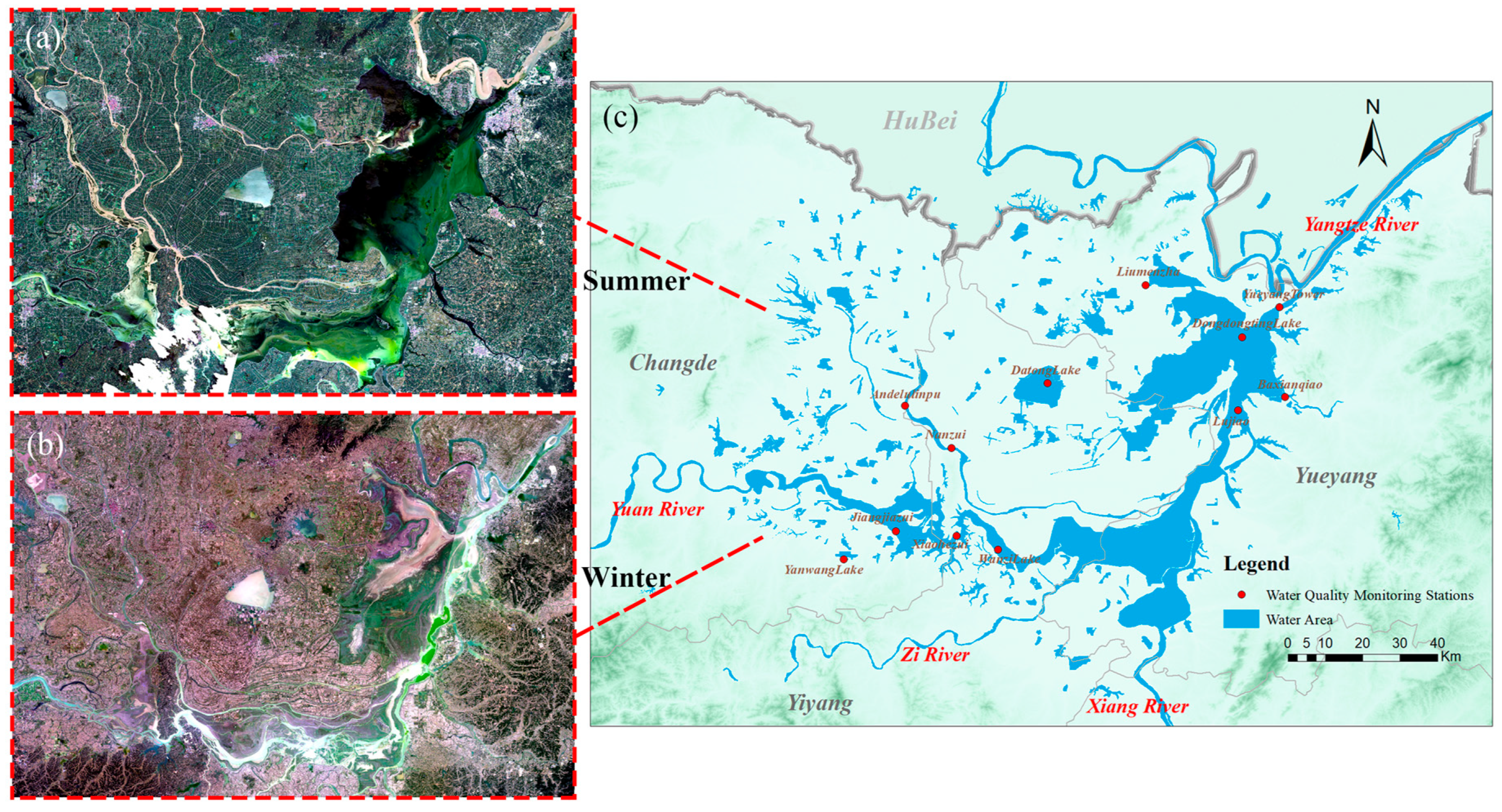
Dongting Lake is situated on the southern bank of the Jingjiang reach in the middle Yangtze River, central China (28°44′–29°35′N, 111°53′–113°05′E; [32]) (Figure 1). The lake lies at the junction of Hunan, Hubei, and Jiangxi Provinces and consists of eight interconnected water systems, including the Xiang, Zi, Yuan, and Li Rivers, along with the East, South, and West Dongting sub-lakes and the Four Outlets system [33]. Covering a surface area of approximately 26,300 km², Dongting Lake is the second largest freshwater lake in China and serves as a critical flood regulation and water storage body in the middle and lower reaches of the Yangtze River [12,13]. It plays an important role in hydrological regulation, flood control, navigation, and maintaining regional ecological balance [34].

Over the past several decades, Dongting Lake has faced increasing ecological stress due to the discharge of industrial, agricultural, and domestic wastewater. The lake has experienced shrinkage and a decline in its water storage and regulation capacity, accompanied by a substantial increase in nutrient inputs, particularly nitrogen and phosphorus [35]. Monitoring data indicate that the single-factor water quality indices for total nitrogen (TN) and total phosphorus (TP) have remained at relatively high levels for a long period, identifying them as the main controlling factors of eutrophication and water quality degradation [36]. The inner lake areas are mostly shallow and characterized by weak hydrodynamic conditions, which limit pollutant dispersion and enhance vulnerability to external and localized pollution sources. Moreover, frequent acid rain caused by atmospheric deposition further aggravates the environmental and ecological stress within the lake basin [37,38].

2.2. Dataset

2.2.1. Satellite Imagery

The hyperspectral data utilized in this study were primarily acquired from Gaofen-5 (GF-5) and Ziyuan-1 (ZY-1), comprising a total of 26 scenes. A dataset was constructed for developing the water quality retrieval model by extracting spectral information from 344 representative sampling points.

The GF-5 satellite is a full-spectrum hyperspectral mission designed for comprehensive atmospheric and terrestrial observation [39]. It offers a swath width of 60 km and a spatial resolution of 30 m. Its Visible and Shortwave Infrared (VSWIR) hyperspectral sensor covers wavelengths from 400 to 2500 nm across 330 spectral channels, with a spectral resolution of 5 nm in the visible and near-infrared regions, making it highly suitable for water quality monitoring.

The ZY-01D and ZY-01E satellites are medium-resolution Earth observation satellites designed for applications such as soil quality mapping [40], water environment monitoring, and vegetation analysis [41]. ZY-01E inherits the mature design of ZY-01D and operates in a networked configuration [42]. Both satellites carry high signal-to-noise VSWIR hyperspectral imagers that acquire 166 bands within 400–2500 nm at a 30 m spatial resolution, providing valuable data for continuous monitoring of water quality.

The Landsat-8 satellite is equipped with the Operational Land Imager (OLI) and the Thermal Infrared Sensor (TIRS). It includes 11 spectral bands, comprising multispectral bands at 30 m resolution and a panchromatic band at 15 m resolution. With a revisit period of 16 days, Landsat-8 enables consistent seasonal coverage and supports long-term global land surface observation.

2.2.2. In Situ Data

In situ water quality data were obtained from the Dongting Lake Ecological and Environmental Monitoring Center in Hunan Province. The dataset includes observations from 12 monitoring sections distributed across Dongting Lake, its inner sub-lakes, and surrounding tributaries, providing a spatially representative overview of water quality variations within the basin (see Figure 1). The 12 fixed monitoring stations are widely distributed across the 26,300 km² Dongting Lake basin, with substantial distances between each station. Given this broad spatial dispersion, the sampling areas do not overlap. All sections are supported by automated surface water monitoring stations, which employ online sensing instruments for high-frequency, continuous, real-time data collection [43].

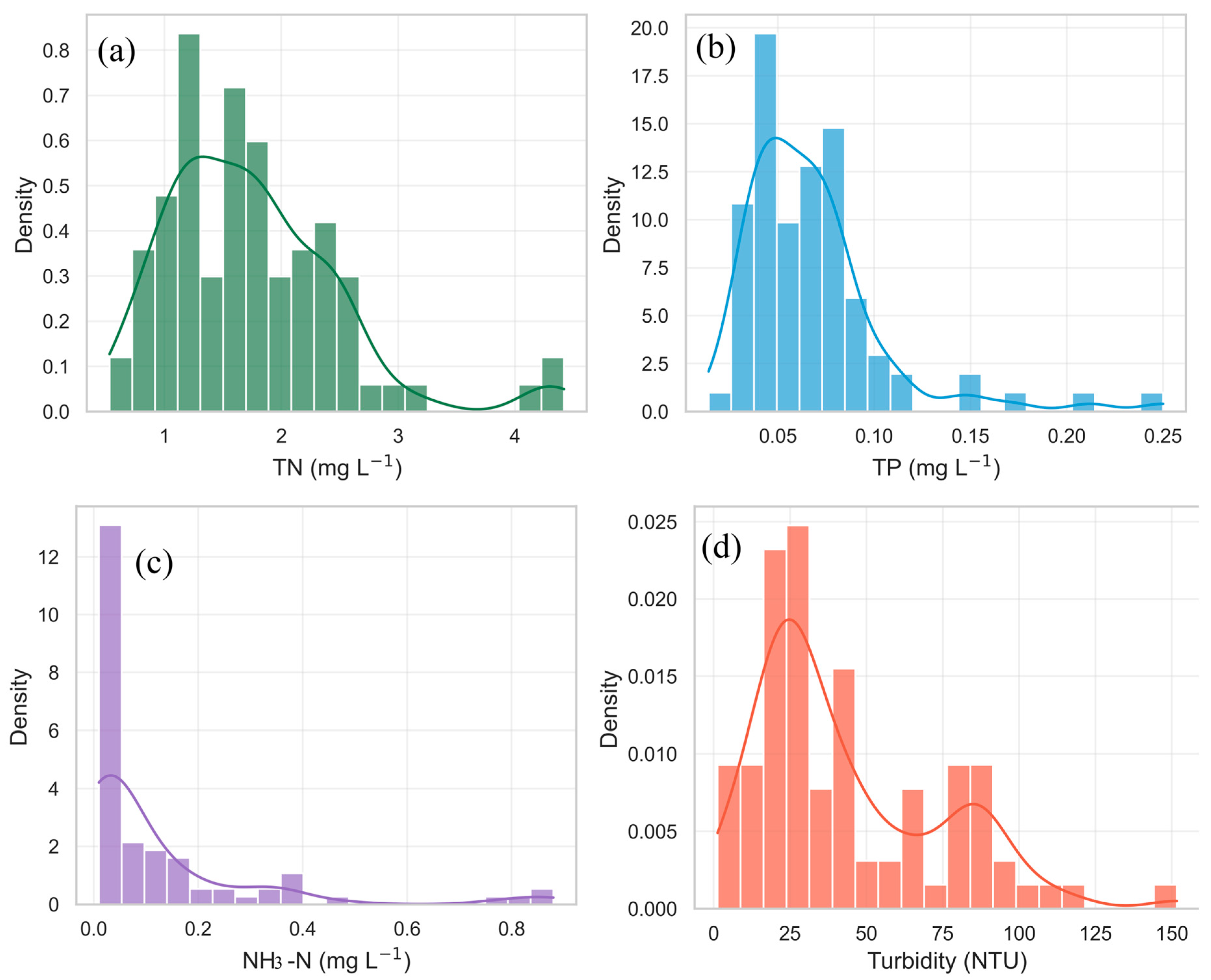
Four typical indicators—Total Nitrogen (TN), Total Phosphorus (TP), Ammonium Nitrogen (NH₃–N), and turbidity—were selected to develop and validate the water quality retrieval models. TN and TP are closely associated with the degree of eutrophication, reflecting the nutrient pollution level of the water body [44], while NH₃–N serves as an important indicator of organic matter decomposition [45]. Turbidity reflects water clarity and light penetration [46]. In total, 344 water quality samples collected between 2022 and 2023 were used to build the dataset for CNN-based water quality retrieval modeling. Histograms illustrating the concentration distributions of the four parameters are presented in Figure 2.

2.2.3. Data Preprocessing

Prior to data matching, all hyperspectral images were preprocessed to ensure temporal and cross-sensor consistency. First, raw digital number (DN) images were reprojected to the WGS84 geographic coordinate system to unify the spatial reference across different sensors. Subsequently, radiometric calibration and atmospheric correction were performed using ENVI 5.6. Radiometric calibration converts sensor-recorded DN values into physically meaningful radiance, enabling quantitative comparisons among images from different periods [47].

Atmospheric correction was conducted using the FLAASH (Fast Line-of-sight Atmospheric Analysis of Spectral Hypercubes) model, which compensates for the effects of scattering and absorption, thereby retrieving the remote sensing reflectance (Rrs) at the top of the atmosphere and minimizing spectral distortions caused by atmospheric and illumination variability [48]. Subsequently, the corrected Rrs images were orthorectified using Rational Polynomial Coefficients (RPCs) to remove geometric distortions introduced by terrain relief, sensor viewing angles, and system errors, ensuring high geometric accuracy [49]. Further geometric registration was performed in ENVI Classic to spatially align all images at the pixel level [50].

To further ensure that the spectral curves used for model training represent physically plausible “pure water” signals, a rigorous sample quality control procedure was implemented. First, abnormal high-reflectance samples were removed using a hard threshold, excluding spectra with reflectance values exceeding 0.2 in the visible and near-infrared bands, thereby eliminating potential contamination from floating vegetation, shoreline debris, or strong specular reflections. Second, sensor malfunction (e.g., dead bands) was identified by applying a sliding window approach, and samples containing five or more consecutive bands with zero reflectance were discarded. Finally, during the sample matching stage, records with missing values were strictly filtered out, and only valid samples with one-to-one correspondence among image acquisition date, sampling site, and in situ water quality measurements were retained, thereby guaranteeing the reliability of the model inputs.

Images of the Dongting Lake region for the summer and winter seasons from 2015 to 2025 were acquired via the Google Earth Engine (GEE) platform. To extract the water boundaries, the Normalized Difference Water Index (NDWI) threshold segmentation method [51] was employed. As a spectral analysis technique, this approach examines the reflective characteristics of imagery across different bands. By conducting mathematical operations on the two bands that exhibit the greatest contrast in reflectance between water and other land cover types, local segmentation was applied to delineate individual water bodies.

3. Methods

3.1. Convolutional Neural Networks

In this study, a convolutional neural network (CNN) was employed to extract hyperspectral image features for estimating the concentrations of TP, TN, NH₃–N, and turbidity. The CNN takes the original hyperspectral data as input and utilizes the backpropagation algorithm to optimize its parameters through a series of operations, including convolution, pooling, and nonlinear activation mapping, thereby deriving representative feature embeddings that are ultimately mapped to the target variables [52]. A typical CNN architecture consists of an input layer, convolutional layers, pooling layers, fully connected layers, and an output layer [53].

The convolutional layers apply learnable kernels to perform convolution on feature maps from the preceding layer, followed by an activation function to produce output feature maps. In this study, the Rectified Linear Unit (ReLU) was adopted as the activation function due to its simplicity and computational efficiency, which enhances the network’s ability to model nonlinear transformations [54]. The pooling layers reduce the dimensionality of feature maps through down sampling while preserving local invariance. This study uses the average pooling function, which calculates the arithmetic mean of all elements in the calculated block as the function output, extracting the mean of the local response of the feature plane. The fully connected layers integrate discriminative local features extracted from convolutional or pooling layers. The backpropagation stage adopts a training parameter update strategy based on gradient descent to minimize the loss function [55].

3.2. CNN with Attention Modules

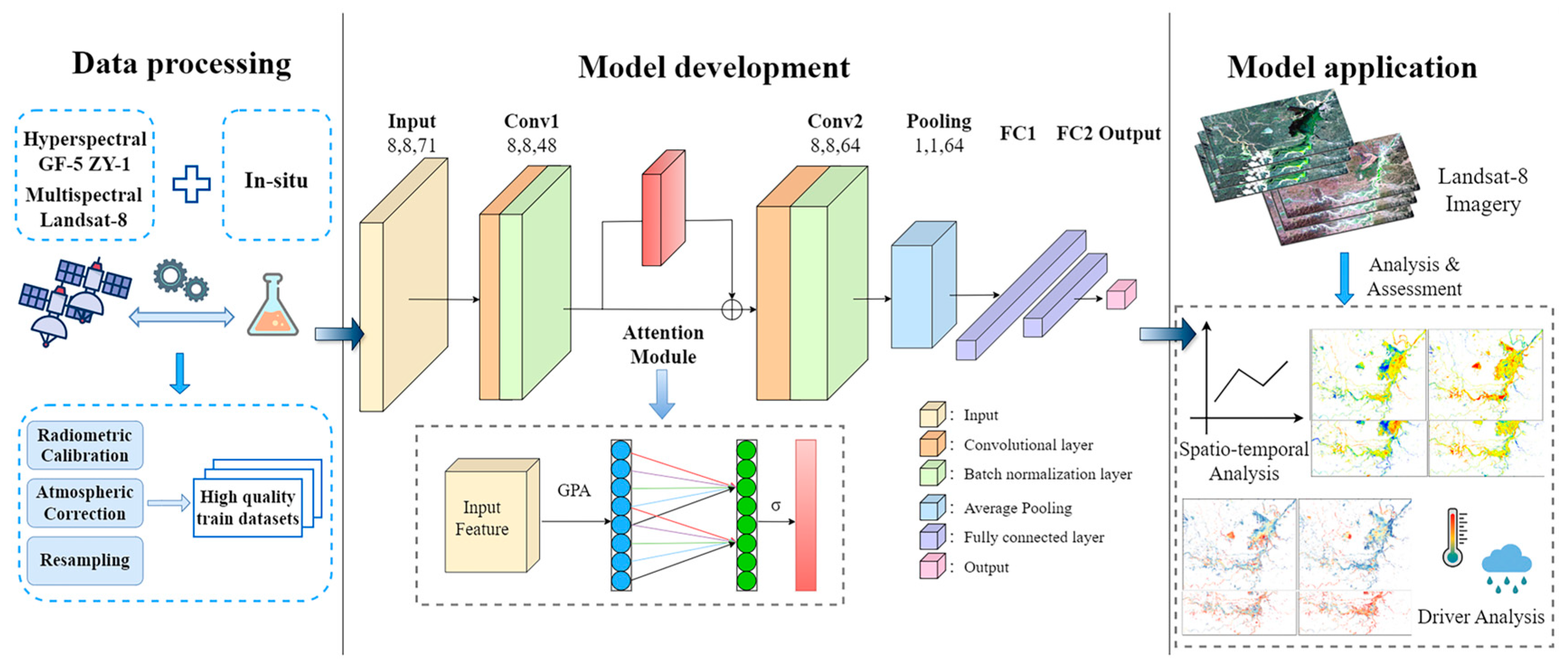
The attention module enhances interpretability by quantifying band importance. Specifically, an Efficient Channel Attention (ECA) module is integrated to increase the sensitivity of the deep learning model to feature channels. The module captures local cross-channel interactions at minimal computational cost, performs no dimensionality reduction, and efficiently models interdependencies across channels using one-dimensional convolution [56]. In this study, a Spectral Attention CNN inversion model was developed for retrieving water quality parameters (see Figure 3). The detailed configuration of the model architecture, including layer functions and output tensor dimensions, is summarized in

Table 1. Detailed architecture of the SA-CNN model. For Landsat imagery, the input band dimension is adjusted to 5, while all other structural parameters remain consistent.

Layer Name	Function	Filter Size	Output Tensor
Input layer	Input bands (Hyperspectral)		$71\times 8\times 8$
Input ECA	Efficient Channel Attention		$71\times 8\times 8$
Convolutional layer 1	Convolutional/ReLu	$3\times 3$	$48\times 8\times 8$
Batch normalization 1	Batch normalization		$48\times 8\times 8$
Convolutional layer 2	Convolutional/ReLu	$3\times 3$	$64\times 8\times 8$
Batch normalization 2	Batch normalization		$64\times 8\times 8$
Feature ECA	Efficient Channel Attention		$64\times 8\times 8$
Global pooling	Adaptive Average Pooling		$64\times 1\times 1$
Dropout 1	Dropout (Rate: 0.4)		$1\times 64$
Fully connected layer 1	Linear/ReLu		$1\times 32$
Dropout 2	Dropout (Rate: 0.4)		$1\times 32$
Fully connected layer 2	Linear (Output)		$1\times 1$

. The input tensor has dimensions 71 × H × W, where 71 denotes the spectral depth (i.e., the number of spectral bands), and H and W represent the spatial height and width of the input image, respectively. The network includes two convolutional layers that progressively extract local spatial–spectral representations. As shown in Table 1, Convolutional layer 1 and 2 utilize $3\times 3$ filters to transform the feature maps into depths of 48 and 64, respectively. To mitigate gradient vanishing caused by early saturation of nonlinear activations during training, batch normalization (BN) [57] was applied after each convolutional layer. BN stabilizes the distribution of layer inputs, keeping activations within the gradient-sensitive region and thereby alleviating gradient instability or disappearance. The BN operation can be expressed as:

$$y_i=\gamma {\displaystyle \frac{x_i-\mu }{\sqrt{{\sigma }^2+\epsilon }}}+\beta$$

(1)

where $x_i$ is the input feature, $\mu$ and $\sigma$ are the batch mean and variance, $\epsilon$ is a small constant to avoid division by zero, and $\gamma$ and $\beta$ are learnable scaling and shifting parameters that restore the representation capability of the model.

Figure 3. The framework of the proposed SA–CNN. (1) Multi-source and in situ data matching, where hyperspectral and multispectral remote sensing data are preprocessed and spatiotemporally matched with in situ data; (2) model development, employing a CNN architecture integrated with an Attention Module to extract key spectral features; and (3) model application, utilizing the trained model to map spatio-temporal water quality distributions using Landsat-8 imagery and analyze driving factors.

Figure 3. The framework of the proposed SA–CNN. (1) Multi-source and in situ data matching, where hyperspectral and multispectral remote sensing data are preprocessed and spatiotemporally matched with in situ data; (2) model development, employing a CNN architecture integrated with an Attention Module to extract key spectral features; and (3) model application, utilizing the trained model to map spatio-temporal water quality distributions using Landsat-8 imagery and analyze driving factors.

Subsequently, a Feature ECA module is applied to the 64-channel feature map, followed by a global adaptive average pooling layer was applied to downsample the overall spatial information, compressing the output to a $64\times 1\times 1$ tensor. A dropout layer with a rate of 0.4 was then employed to mitigate overfitting [58]. Dropout is a widely used regularization technique: by randomly dropping out a fraction of neurons during forward propagation, it effectively forms different sub-network structures each time and enhances the generalization ability of the network. Finally, the convolutional feature map is subsequently flattened and fed into a fully connected (FC) regression module, and the output of the FC layer is of dimension 1 × 1, i.e., the predicted value of the water-quality parameter. This output is passed into the loss function, defined as the mean squared error (MSE):

$$\mathrm{MSE}={\displaystyle \frac{1}{n}}\sum _{i=1}^N{\left(y_i-\widehat{y_i}\right)}^2$$

(2)

where $y_i$ and $\widehat{y_i}$ represent the observed and estimated values, respectively. The network parameters were optimized via backpropagation based on the gradient descent algorithm, adjusting the parameters in the direction that minimizes the loss through the chain rule [59].

3.3. Performance Evaluation

Retrieval models for water quality parameters were developed using in situ measurements and corresponding hyper spectral data. All samples were randomly divided into training and validation subsets, with 75% of the samples (N = 258) used for model construction and parameter optimization, and the remaining 25% (N = 86) reserved for independent validation to assess the model’s generalization ability and predictive accuracy. Model accuracy was quantitatively assessed using three statistical metrics: the coefficient of determination ($R^2$), root mean square error (RMSE), and mean absolute error (MAE) [60], which are defined as follows:

$$R^2=1-{\displaystyle \frac{{\sum }_{i=1}^N{\left(\widehat{x_i}-x_i\right)}^2}{{\sum }_{i=1}^N{\left(x_i-\overline{x}\right)}^2}}$$

(3)

$$\mathrm{RMSE}=\sqrt{{\displaystyle \frac{{\sum }_{i=1}^N{\left(\widehat{x_i}-x_i\right)}^2}{N}}}$$

(4)

$$\mathrm{MAE}={\displaystyle \frac{1}{N}}\sum _{i=1}^N\left|\widehat{x_i}-x_i\right|$$

(5)

where $\widehat{x_i}$ and $x_i$ represent the predicted and observed concentrations of the water quality parameter for the i-th sample, respectively, $\overline{x}$ is the mean of the observed values, and N is the total number of samples. A higher $R^2$ value and lower RMSE and MAE values indicate better model performance.

4. Results

4.1. Training and Performance of the Algorithm

During model training, all parameter settings were optimized considering both the data scale and the convergence characteristics of the network. The input size was defined as an 8 × 8 patch, which ensured sufficient neighborhood feature extraction while avoiding noise accumulation and excessive computational cost associated with larger window sizes. The Adam optimizer was employed with a learning rate of 0.001 and a weight decay of $1\times {10}^{-5}$ to suppress overfitting. The batch size was set to 16, and the maximum number of iterations was 100 epochs. An early stopping strategy (patience = 15) was also applied to terminate training when the validation loss failed to decrease over a prolonged period. For data preprocessing, both inputs and outputs were normal ized using Min–Max scaling. In addition, data augmentation techniques such as random rotation and flipping were applied to expand the training dataset by approximately threefold, thereby improving the robustness and generalization capability of the model.

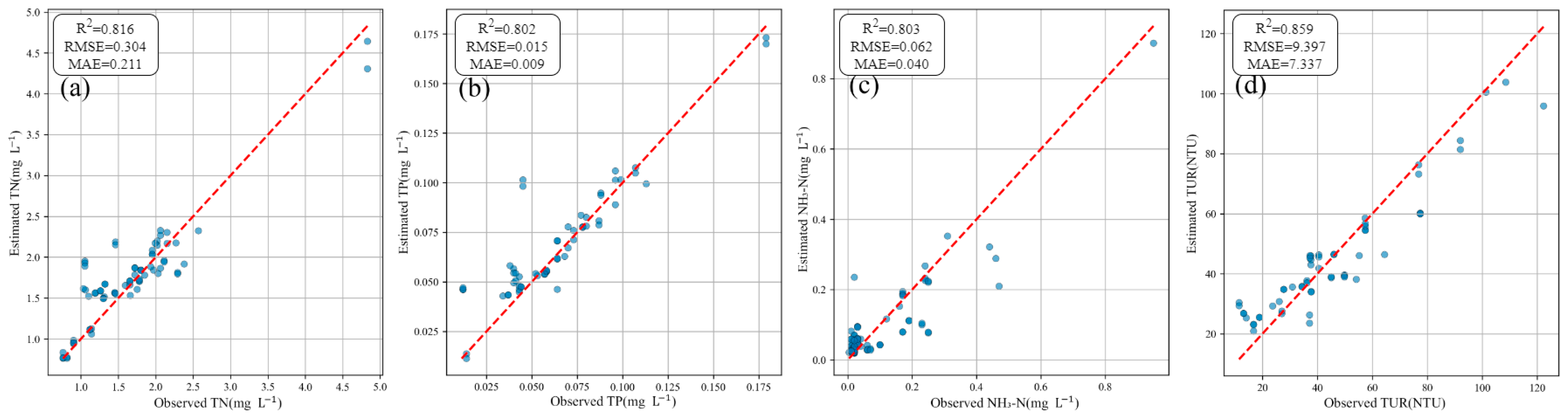
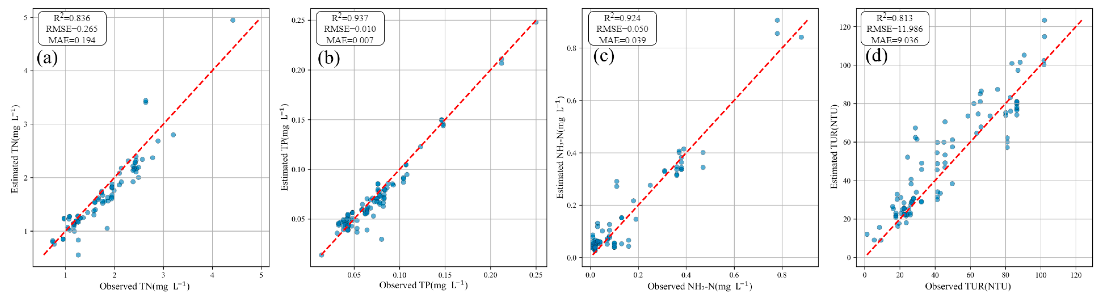
The performance of the SA–CNN retrieval model was evaluated using an independent validation dataset. Figure 4 illustrates the model performance on the hyperspectral dataset, where the best predictive capability was observed for Total Phosphorus (TP) with an $R^2$ of 0.94 (Figure 4b), followed by NH₃–N with an $R^2$ of 0.92 (Figure 4c). The $R^2$ values for Total Nitrogen (TN) and turbidity were 0.84 and 0.81 (Figure 4a–d), respectively. These results demonstrate that the proposed model possesses high stability and reliability in predicting concentrations of TN, TP, NH₃–N, and turbidity.

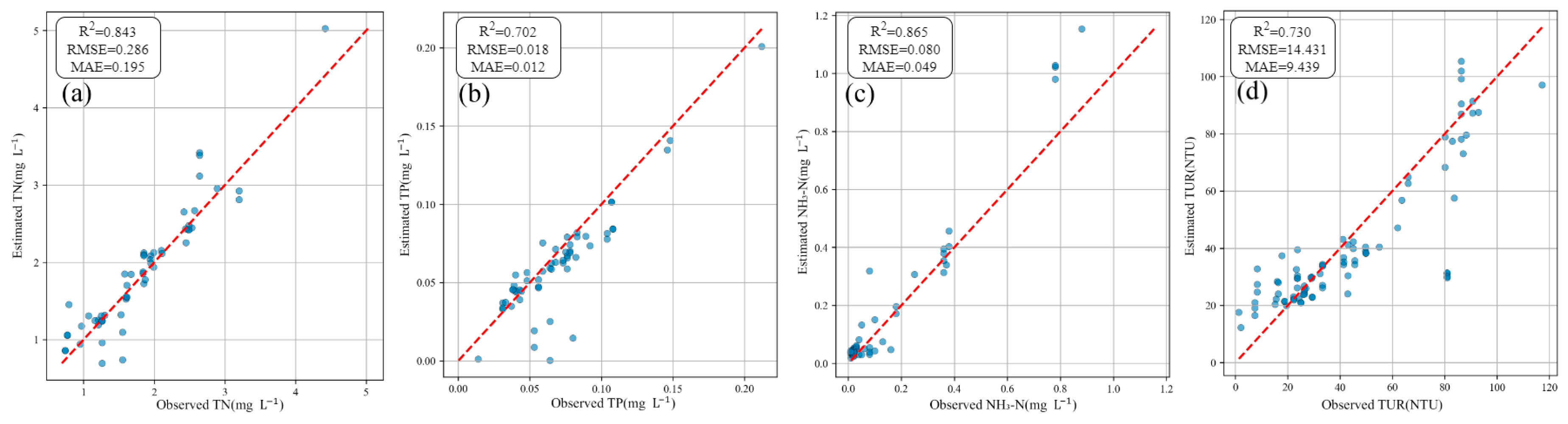
Furthermore, a specific temporal generalization experiment was conducted to evaluate the stability of the model across different years. To achieve this, samples from 2022 and a portion of 2023 were designated for training and validation, while the remaining 2023 data were used as an independent, unseen test set. Given the relatively limited sample size, this strategy aimed to balance the need for temporal validation with the requirement for sufficient training data to prevent overfitting. As shown in Figure 5, the SA–CNN model demonstrates robust performance across all parameters even when tasked with predicting values from a distinct year. Specifically, the NH₃–N and TN models exhibited the highest consistency with $R^2$ values of 0.865 and 0.843, respectively. Although the dataset scale poses challenges for long-term prediction, these results suggest that the integrated ECA attention mechanism and data augmentation strategies effectively enhance the model’s capability to handle inter-annual spectral variability.

4.2. Performance Comparison with Machine Learning Model

In this study, the performance of the SA–CNN model was evaluated through a comparative analysis with both traditional machine learning methods and some deep learning architectures. The retrieval accuracy of XGBoost, Random Forest (RF), Stacking ensemble learning, Transformer, and U-Net was evaluated, with the results summarized in

Table 2. Performance metrics associated with TN, TP, NH₃–N, and turbidity retrievals. (SA-CNN highlights the best performance in bold.).

Model	Metrics	TN	TP	NH3–N	Turbidity
XGBoost	$R^2$	0.604	0.792	0.731	0.688
	$RMSE$	0.557	0.023	0.118	18.03
	$MAE$	0.326	0.013	0.068	10.859
RF	$R^2$	0.518	0.692	0.658	0.597
	$RMSE$	0.614	0.028	0.133	20.495
	$MAE$	0.378	0.018	0.081	13.372
stacking	$R^2$	0.746	0.860	0.762	0.709
	$RMSE$	0.445	0.019	0.111	17.41
	$MAE$	0.298	0.015	0.066	10.856
Transformer	$R^2$	0.790	0.825	0.879	0.759
	$RMSE$	0.291	0.016	0.063	13.627
	$MAE$	0.181	0.013	0.037	8.179
U-Net	$R^2$	0.806	0.867	0.880	0.881
	$RMSE$	0.280	0.014	0.065	9.573
	$MAE$	0.189	0.011	0.048	7.214
CNN Without ECA	$R^2$	0.809	0.900	0.923	0.628
	$RMSE$	0.313	0.013	0.058	17.122
	$MAE$	0.192	0.010	0.041	11.709
SA-CNN	$R^2$	0.836	0.937	0.924	0.813
	$RMSE$	0.265	0.010	0.050	11.986
	$MAE$	0.194	0.007	0.039	9.036

. The comparison shows that the SA–CNN model consistently outperformed all benchmark models across the majority of water quality parameters. Specifically, its $R^2$ values for TN, TP, NH₃–N, and turbidity reached 0.84, 0.94, 0.92, and 0.81, respectively, significantly exceeding the baseline models. Concurrently, the corresponding RMSE and MAE values for the SA–CNN model generally remained at the lowest levels among all tested methods.

These results indicate that the proposed model effectively captures the nonlinear relationships between hyperspectral reflectance and water quality parameters, demonstrating strong generalization ability and robustness. While advanced architectures like Transformer and U-Net showed competitive performance, particularly in capturing long-range dependencies or spatial features, they did not reach the overall precision of the SA-CNN in this specific task. The RF model performed relatively weakly, with significantly lower prediction accuracy across all indicators. The Stacking model, however, achieved higher overall precision than any single traditional machine learning model, highlighting the advantage of ensemble learning for certain parameters. In summary, the SA–CNN model consistently outperformed both conventional algorithms and complex deep learning frameworks across the majority of water quality indicators, confirming that integrating spectral attention with CNN provides robust solutions for complex aquatic remote sensing tasks. The incremental improvement in precision over the “CNN Without ECA” model further highlights the efficacy of the ECA attention module in capturing critical spectral features for more accurate water quality estimation.

4.3. Application of the Model to Landsat Data

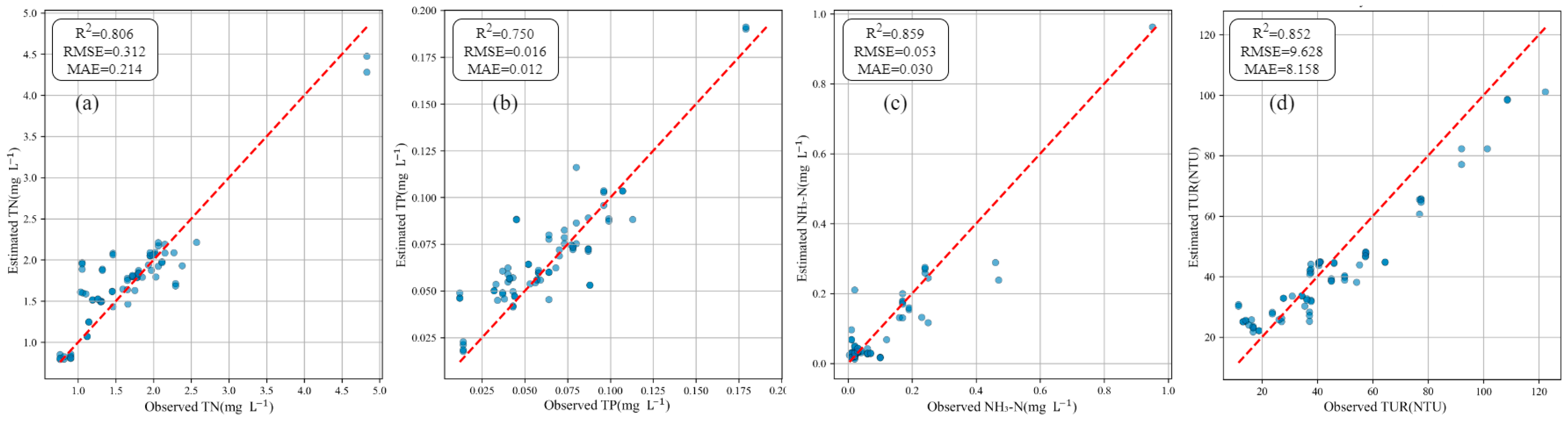
By analyzing the band weights extracted for the four water quality parameters, it was found that the sensitive bands for the three non-optically active parameters are primarily located between 760 nm and 900 nm, while those for turbidity are situated around 900–1000 nm and 400 nm. Regarding the differences in Spectral Response Functions (SRFs) between hyperspectral and Landsat sensors, it is worth noting that Landsat’s multispectral bands have wider bandwidths compared to the narrow, continuous bands of hyperspectral data. In this study, we mapped the hyperspectral weights to the Landsat bands based on their central wavelength alignment. Since the weight mapping process focuses on transferring the relative importance and sensitivity distribution of wavelengths rather than absolute spectral radiance, this central-wavelength-based mapping effectively retains the underlying physical mechanism for target water quality parameters while accommodating the spectral resolution discrepancy. Using this as prior information, the SA–CNN model was trained and evaluated on the Landsat dataset (Figure 6). The results indicate that the model performed best for turbidity ($R^2$ = 0.86), followed by TN ($R^2$ = 0.82), with both TP and NH₃–N reaching an $R^2$ of 0.80. To evaluate the effectiveness of this transfer mechanism, we conducted a comparative experiment with and without the weighted mapping strategy (i.e., before (Figure 7) and after (Figure 6) applying weight transfer). The results show that the model using weighted mapping achieved significant performance improvements across TN, TP, and turbidity. Notably, the improvement for TP was the most significant, with its R² increasing from 0.75 to 0.80 This indicates that the weighted transfer distribution can effectively reduce the differences between different sensors and guide the model to focus on the most relevant spectral features.

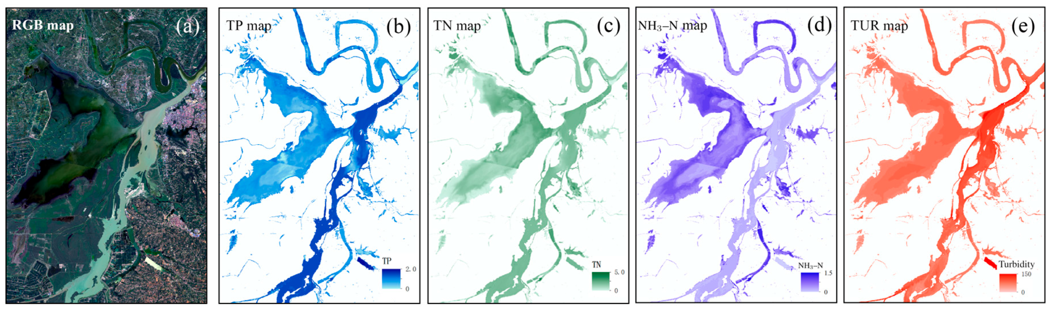
To visually demonstrate the applicability of the model, Figure 8 displays the spatial distributions of various water quality parameters in East Dongting Lake during the summer of 2025. The retrieval results reveal distinct spatial heterogeneity, with high-concentration areas for all four parameters predominantly located along major inlet rivers and flow channels, whereas the open lake area exhibits relatively lower concentrations. This pattern aligns well with the turbid features observed in the RGB composite image, further confirming the robustness of the model in capturing water quality variations.

4.4. Spatial and Temporal Variations of Dongting Lake from 2015 to 2025

4.4.1. Interannual Variations

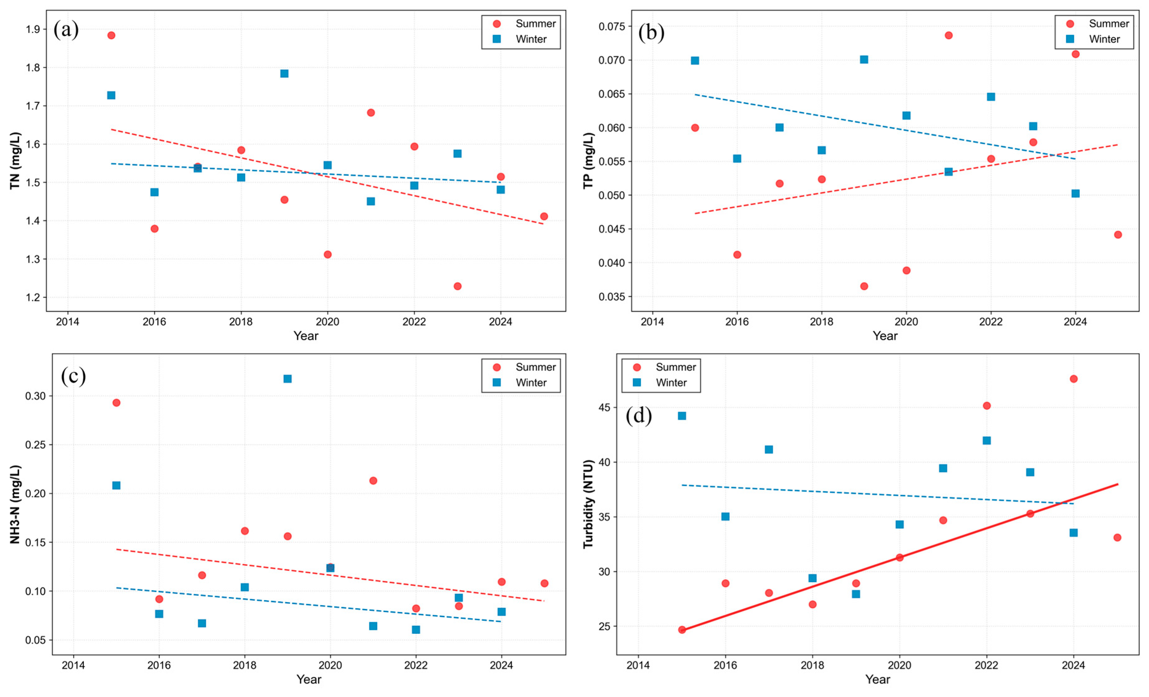
Using the proposed retrieval model, spatial distributions of total nitrogen (TN), total phosphorus (TP), ammonia nitrogen (NH₃–N), and turbidity were mapped for Dongting Lake. Images from July–September and November–January were selected to represent summer and winter seasons, respectively, spanning from 2015 to 2024 (including summer 2025). Based on the retrieved concentrations, seasonal averages were calculated for each year, and Sen’s Slope was employed to quantify inter-annual trends (Figure 9). Overall, over the past decade, all water quality parameters in winter exhibited a fluctuating downward trend with limited variability. In summer, TN and NH₃–N concentrations generally trended downward with fluctuations (Figure 9a,c), whereas TP and turbidity showed an overall increasing trend (Figure 9b–d).

During the summer, concentrations of TN, TP, and NH₃–N all exhibited a downward trend from 2015 to 2020, followed by an abrupt surge in 2021 before gradually declining again. Specifically, the peak concentration of TP occurred in 2021 at 0.074 mg·L⁻¹, while the minimum was recorded in 2019 at 0.037 mg·L⁻¹. For TN and NH₃–N, the highest concentrations were observed in 2015, at 1.88 mg·L⁻¹ and 0.29 mg·L⁻¹, respectively. After a period of fluctuating decline, both parameters rebounded sharply in 2021, reaching 1.68 mg·L⁻¹ and 0.21 mg·L⁻¹, before resuming a downward trajectory. In contrast, turbidity showed a pronounced upward trend until 2022, after which it began to decrease. During winter, the concentrations of TN, TP, and NH₃–N in Dongting Lake exhibited fluctuating but overall declining trends. The maximum concentrations of TN and NH₃–N both occurred in 2019, reaching 1.78 mg·L⁻¹ and 0.16 mg·L⁻¹, respectively. The minimum TN concentration (1.45 mg·L⁻¹) was recorded in 2021, while NH₃–N reached its lowest level (0.06 mg·L⁻¹) in 2022. Winter turbidity exhibited considerable year-to-year variation with a post-2022 decreasing tendency, though no statistically significant overall trend was detected.

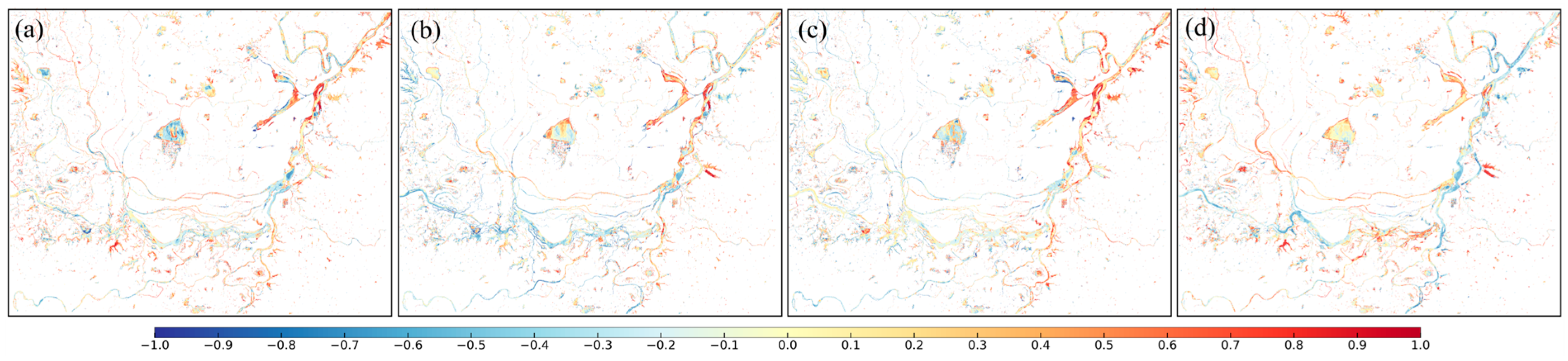
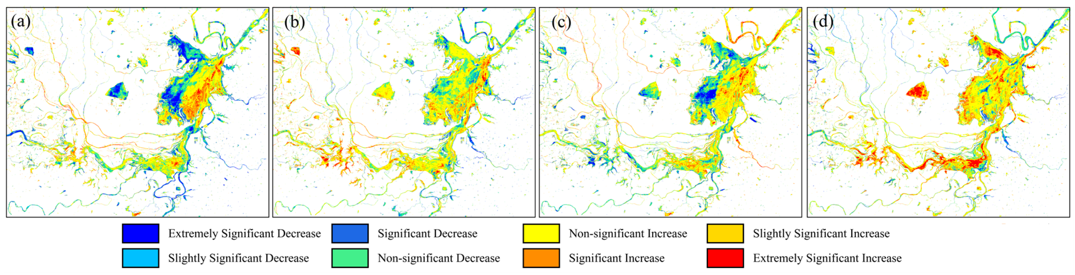
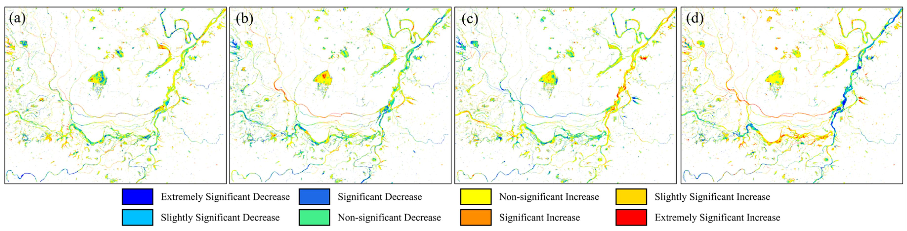
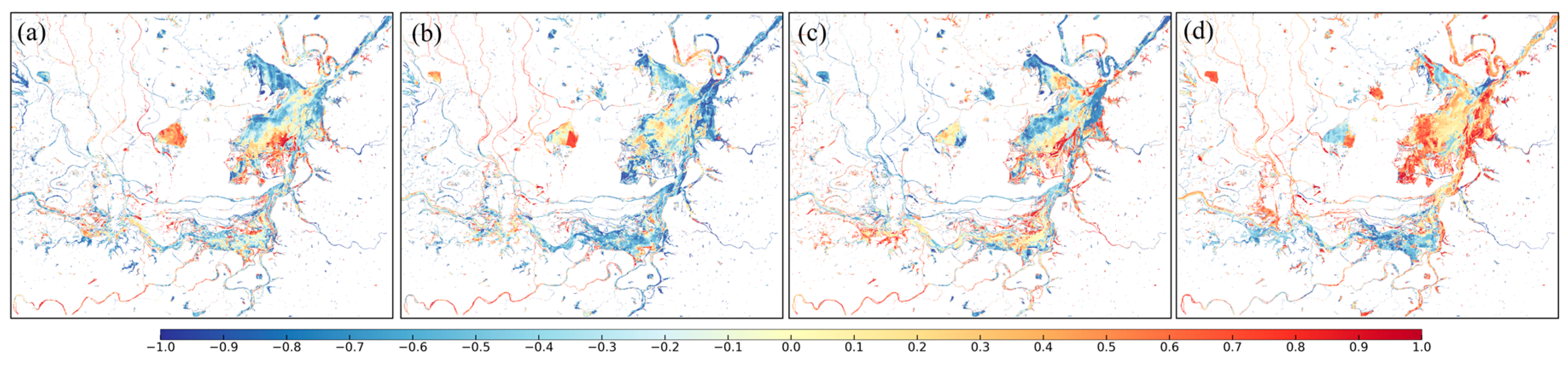
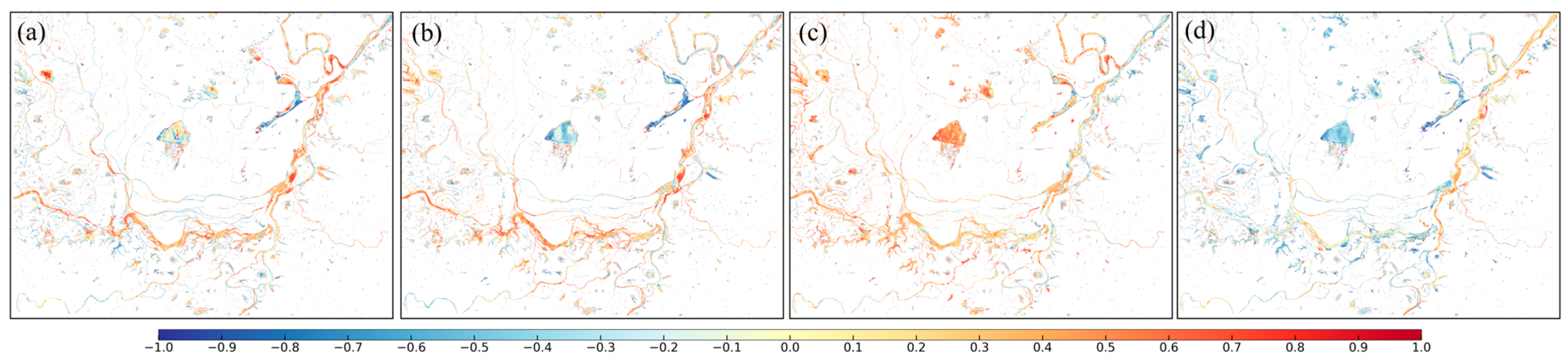
The Mann–Kendall (M-K) test was employed to effectively characterize the variation trends at a pixel-wise scale. Pixels identified as water bodies for more than five years were defined as valid pixels, upon which the M-K test and Sen’s Slope were performed to reflect the spatial distribution characteristics of water quality trends in Dongting Lake (Figure 9 and Figure 10). In both summer and winter, the four parameters predominantly exhibited non-significant increases or decreases. During summer, TN and NH₃–N showed significant downward trends in the western part of East Dongting Lake (Figure 10a,c), whereas significant increases were observed in the eastern section; South and West Dongting Lakes were primarily characterized by non-significant variations. TP exhibited significant upward trends in eastern East Dongting Lake, near the Yangtze River inlets, and in West Dongting Lake, with significant decreases observed only along the western fringes (Figure 10b). Turbidity mainly showed non-significant to significant increases, with the latter being particularly evident in South Dongting Lake and inner lakes such as Datong Lake (Figure 10d). In winter, during the low-water period, concentrations of TN, TP, and NH₃–N were dominated by non-significant trends (Figure 11a–c). However, turbidity in East Dongting Lake decreased significantly (Figure 11d), while TP in inner-lake regions exhibited a significant increase.

4.4.2. Seasonal Variation

Dongting Lake, situated in the middle reaches of the Yangtze River Plain, exhibits typical East Asian monsoon climate characteristics, with hot and rainy summers where precipitation and temperature peak concurrently. As a typical seasonal lake, its surface area fluctuates substantially throughout the year, showing significant differences in lake morphology between the wet and dry seasons. This study analyzed water quality variations in Lake Dongting across two contrasting seasons: the wet (summer) and dry (winter) periods. Over the past decade, NH₃–N concentrations consistently remained higher in summer than in winter. Before 2019, TN concentrations were generally higher in summer than in winter, but after 2019, TN levels tended to be slightly higher in winter than in summer. TP and turbidity exhibited similar patterns, with winter concentrations slightly exceeding summer levels prior to 2024. However, in the summer of 2021, TP concentrations were significantly higher than in winter, which was driven by the complex interplay between high-intensity human activities and the subsequent implementation of watershed management policies.

5. Discussion

5.1. Strengths of the SA–CNN Model

The SA–CNN model achieved high accuracy in the inversion of total nitrogen, total phosphorus, ammonia nitrogen, and turbidity. By mapping the band weights extracted from the hyperspectral model to the corresponding band ranges of Landsat multispectral data, the model was further transferred to multispectral datasets for training. The resulting inversion accuracy was slightly higher than that obtained without prior band-weight information and was markedly superior to that of traditional machine learning models.

Furthermore, the incorporation of batch normalization and dropout techniques effectively mitigated overfitting issues commonly encountered in small-sample datasets, significantly enhancing the model’s stability and generalization capability. The proposed model effectively integrates the fine and information-rich spectral features of hyperspectral data with the broad temporal coverage and strong temporal continuity of Landsat data, thereby achieving complementarity between spectral and temporal information. This integration enables the characterization of spatial heterogeneity and interannual variability in Dongting Lake over the past decade, supporting dynamic monitoring and continuous assessment of lake water quality. When the input data encompass a larger extent of lake waters, the model is also capable of providing reasonable spatiotemporal monitoring and evaluation for different regions. Overall, the model offers a reliable approach for revealing the spatiotemporal evolution patterns of lake water quality and provides technical support for watershed-scale ecological environmental monitoring and pollution management.

5.2. Factors and Mechanisms Influencing Water Quality in Dongting Lake

5.2.1. Impact of Meteorological Factors

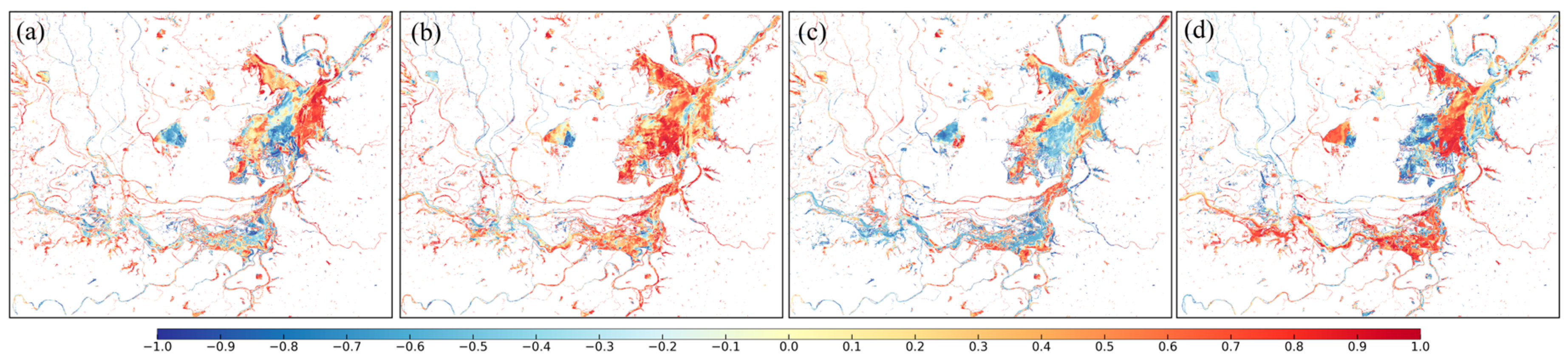
Precipitation and temperature are pivotal meteorological factors in aquatic environments. Precipitation is intrinsically linked to surface runoff and serves as a primary driver of river discharge and lake water levels, thereby directly modulating the concentrations of nitrogen, phosphorus, and turbidity. Temperature significantly influences the proliferation of algae, whose biological uptake and metabolic activities directly affect the nutrient dynamics of nitrogen and phosphorus in the water column [61]. In this study, total precipitation and temperature data for the Dongting Lake region were acquired to calculate seasonal averages for summer and winter. Furthermore, the Pearson correlation coefficients between these meteorological variables and the four water quality parameters (TN, TP, NH₃–N, and turbidity) were computed to generate spatial correlation maps (Figure 11, Figure 12, Figure 13 and Figure 14).

Overall, a negative correlation was observed between summer precipitation and the concentrations of nitrogen and phosphorus (Figure 12a,c). Increased precipitation raises lake water levels, thereby exerting a dilution effect that reduces nutrient concentrations. In contrast, turbidity showed a positive correlation with precipitation (Figure 12d). Increased precipitation enhanced surface runoff and erosion processes, promoting the transport of suspended sediments and other materials into lakes and rivers [62], thereby increasing water turbidity. Spatially, TN and NH₃–N concentrations in the southern marginal area of East Dongting Lake and the northern marginal area of South Dongting Lake were positively correlated with precipitation. The eastern and southern parts of the lake region are dominated by agricultural land; thus, increased precipitation facilitates the transport of nitrogen and phosphorus from agricultural areas into the lake via runoff, resulting in elevated concentrations of total nitrogen and ammonia nitrogen. In winter, all four water quality parameters showed an overall positive correlation with precipitation. Winter in Dongting Lake corresponds to the dry season, during which the lake surface area shrinks and the system exhibits more river-like characteristics (Figure 13). Under such conditions, increased precipitation does not substantially raise water levels but instead enhances the input of nitrogen, phosphorus, and sediments from surrounding agricultural lands into the lake, leading to increased concentrations of TN, TP, NH₃–N, and turbidity.

Elevated temperatures enhance biological and microbial activities and accelerate metabolic rates, thereby increasing the concentrations of nutrients such as nitrogen and phosphorus in the water. As shown in the figure, during summer, TN, TP, NH₃–N, and turbidity in Dongting Lake were predominantly positively correlated with temperature (Figure 14). Among these parameters, TP exhibited a significant positive correlation with temperature (Figure 14b), as the release of phosphorus in lakes is highly dependent on temperature and redox conditions. Elevated temperatures accelerate microbial metabolism and promote the development of hypoxic conditions, which in turn enhance phosphorus release and increase TP concentrations. In contrast, TN and NH₃–N concentrations in the central lake region were less sensitive to temperature variations than phosphorus (Figure 14a,c). Although higher temperatures tend to increase TN concentrations, processes such as ammonia volatilization may also occur, resulting in a weaker over all sensitivity of nitrogen species to temperature compared with phosphorus. There is no direct relationship between turbidity and temperature; however, increasing temperature promotes algal growth, and the associated increase in algal cells and organic particulates can indirectly lead to higher turbidity (Figure 14d). During winter, water quality parameters in Lake Dongting showed positive correlations with temperature in East Dongting Lake, although the overall correlations were not statistically significant (Figure 15).

5.2.2. Impact of Human Activities

Dongting Lake receives in flows from the Xiang, Zi, Yuan, and Li Rivers, as well as from the Yangtze River, and pollutants from these sources ultimately converge into the lake. Both TN and TP concentrations were relatively high in the western part of Dongting Lake, while elevated TP levels were also observed in the southern part. The Xiang and Yuan Rivers serve as major inlets for the southern and western regions of the lake, respectively. The Yuan River, a tributary of the Yangtze in the Dongting Lake basin, originates in Duyun, Guizhou, where abundant phosphate resources and numerous phosphate chemical enterprises are present. Consequently, TP concentrations in the Yuan River are typically high due to upstream industrial effluents. Similarly, the Xiang River, flowing through major urban centers such as Yueyang, Changsha, and Xiangtan, is heavily influenced by dense populations and industrial activities, with substantial nitrogen and phosphorus loads entering Dongting Lake from domestic and industrial wastewater [63].

Besides upstream river inflows, water quality in Dongting Lake is also influenced by local sources of pollution. The lake region, covering Yiyang, Changde, and Yueyang, receives direct discharges of pollutants generated within these cities [64]. Moreover, as a key area for poultry and livestock farming, the rapid expansion of animal husbandry contributes large amounts of manure to the lake, serving as a primary source of total phosphorus. The seasonal discrepancy observed in the total phosphorus (TP) concentration in Dongting Lake during 2021 can be largely attributed to the interaction between intensive anthropogenic activities and the subsequent implementation of watershed management policies. According to the Hunan Statistical Yearbook, the effective irrigation area and the total crop sown area in the Dongting Lake region expanded from $1071.94 \mathrm{kha}$ and $2563.69 \mathrm{kha}$ in 2020 to $1098.61 \mathrm{kha}$ and $2581.55 \mathrm{kha}$ in 2021, respectively, which concomitantly increased the application of agricultural fertilizers. Furthermore, intensive aquaculture operations—such as those in Hanshou County, which covers approximately $16.4 \mathrm{kha}$ ($\mathrm{246,000} \mathrm{mu}$) of aquaculture water surface and serves as a major aquatic product production base—discharged considerable volumes of untreated wastewater containing high concentrations of nutrients due to excessive bait and fertilizer usage, leading to severe localized ecological pressure. To mitigate this degradation, the Hunan Provincial Government officially launched the Dongting Lake Total Phosphorus Reduction Campaign in 2021. Following the strict enforcement of phosphorus restrictions and abatement interventions, the TP concentration exhibited a significant decrease by the winter of 2021 and the summer of 2022. This trend demonstrates the critical role of anthropogenic interventions in curtailing nutrient loading and facilitating short-term water quality improvement.

5.2.3. Limitations and Prospects of the Model

While the SA–CNN model performed well for most indicators, several limitations remain. The spatiotemporal coverage of the training samples was limited, with insufficient samples for certain years and lake regions. Specifically, a temporal gap exists between the in situ data collection (2022–2023) and the long-term trend analysis starting from 2015. Since no historical in situ data were available for the 2015–2021 period, the accuracy of these historical reconstructions relies on the model’s temporal transferability, which introduces uncertainty regarding its performance under varying historical hydrological conditions. Consequently, the model exhibits some sensitivity to the training dataset [65]. When applied to other water bodies or under extreme water quality scenarios, prediction accuracy may decline, and generalization capacity could be limited. This result highlights a common limitation of data-driven models in remote sensing applications, where models trained on limited temporal samples struggle to generalize across years [66]. Additionally, the quantitative impact of the uneven distribution of NH₃–N samples—where low-concentration values predominate—leads to considerable uncertainty in high-concentration estimates.

Table 3. Evaluation of NH₃–N inversion performance across different concentration intervals.

Concentration Interval (g/mL)	Sample Size (n)	Proportion	${\mathit{R}}^2$	RMSE	MAE
$0\sim 0.2$	75	79.8%	0.4851	0.0328	0.0226
$0.2\sim 0.6$	17	18.1%	0.3686	0.0399	0.0301
$>0.6$	3	2.1%	0.3404	0.0383	0.0360

presents the quantitative evaluation of the model’s inversion performance across different concentration intervals. In the validation dataset, the majority of samples are concentrated in the low-concentration interval ($0\sim 0.2 \mathrm{g}/\mathrm{mL}$), accounting for $79.8\%$ of the total data, whereas the medium ($0.2\sim 0.6 \mathrm{g}/\mathrm{mL}$) and high ($>0.6 \mathrm{g}/\mathrm{mL}$) intervals represent only $18.1\%$ and $2.1\%$ of the dataset, respectively. The statistical results indicate that the model achieved the best performance in the low-concentration range, with an $R^2$ of 0.458 and the lowest error ($\mathrm{RMSE}=0.0328$, $\mathrm{MAE}=0.0226$). As the concentration increases and the sample size decreases, the model’s inversion accuracy gradually declines. This discrepancy indicates that the higher proportion of low-concentration samples leads to a more robust learning performance for lower values, while the model is slightly less sensitive to the less frequent high-concentration values. Therefore, more balanced sampling or data augmentation is needed in future applications to improve the robustness of high concentration prediction.

In future work, we will consider employing spectral convolution or sensor-specific relative spectral response curves to perform a more rigorous transformation of the hyperspectral data to match the Landsat SRF profile, thereby further improving the robustness of multi-source transfer learning. Furthermore, future research could expand the temporal and spatial coverage of the dataset, particularly by incorporating cross-year samples or conducting long-term time-series validation to further justify model migration. Moreover, incorporating additional hyperspectral data sources, such as UAV- or airborne-based sensors, would facilitate cross-validation of model consistency under varying acquisition platforms.

6. Conclusions

The SA–CNN model efficiently captures high-dimensional spectral features, significantly improving the retrieval accuracy of non-optical water quality parameters. Its stability and generalization ability outperform those of traditional ma chine learning methods and single CNN models. By using hyperspectral band weight mapping as prior information, the model effectively enhances the retrieval performance of Landsat multispectral data, successfully integrating the fine spectral details of hyperspectral imagery with the long-term temporal coverage of multispectral observations. Analysis of the spatiotemporal variations and driving factors of water quality parameters in Dongting Lake over the past decade indicates that the overall water quality has remained relatively stable, although there are localized risks of deterioration. In particular, total phosphorus pollution during summer and the increasing turbidity in the inner lakes exhibit notable upward trends. Precipitation exerts a dilution effect on nitrogen and phosphorus in summer, whereas in winter, it tends to contribute to pollutant inflow. Moreover, rising temperatures significantly promote phosphorus concentration, and human activities also exert certain impacts on lake water quality. The model shows some bias in predicting low concentrations of ammonium nitrogen; therefore, future work should expand the dataset with extreme water quality samples to further enhance the model’s robustness and applicability.

References

1. Bhateria, R.; Jain, D. Water quality assessment of lake water: A review. Sustain. Water Resour. Manag. 2016, 2, 161–173. [Google Scholar] [CrossRef]
2. Vasistha, P.; Ganguly, R. Water quality assessment of natural lakes and its importance: An overview. Mater. Today Proc. 2020, 32, 544–552. [Google Scholar] [CrossRef]
3. Juma, D.W.; Wang, H.; Li, F. Impacts of population growth and economic development on water quality of a lake: Case study of lake victoria kenya water. Environ. Sci. Pollut. Res. 2014, 21, 5737–5746. [Google Scholar] [CrossRef]
4. Wang, L.; Zhang, J.; Wang, Y.; Song, X.; Sun, Z. Artificial intelligence reshapes river basin governance. Sci. Bull. 2025, 70, 1564–1567. [Google Scholar] [CrossRef] [PubMed]
5. Wang, H.; He, W.; Zhang, Z.; Liu, X.; Yang, Y.; Xue, H.; Xu, T.; Liu, K.; Xian, Y.; Liu, S.; et al. Spatio-temporal evolution mechanism and dynamic simulation of nitrogen and phosphorus pollution of the yangtze river economic belt in china. Environ. Pollut. 2024, 357, 124402. [Google Scholar] [CrossRef]
6. Parinet, B.; Lhote, A.; Legube, B. Principal component analysis: An appropriate tool for water quality evaluation and management—Application to a tropical lake system. Ecol. Modell. 2004, 178, 295–311. [Google Scholar] [CrossRef]
7. Grizzetti, B.; Bouraoui, F.; Billen, G.; van Grinsven, H.; Cardoso, A.C.; Thieu, V.; Garnier, J.; Curtis, C.; Howarth, R.W.; Johnes, P. Nitrogen as a threat to european water quality. In European Nitrogen Assessment; Cambridge University Press: Cambridge, UK, 2011; pp. 379–404. [Google Scholar]
8. Giardino, C.; Brando, V.E.; Dekker, A.G.; Strömbeck, N.; Candiani, G. Assessment of water quality in lake garda (italy) using hyperion. Remote Sens. Environ. 2007, 109, 183–195. [Google Scholar] [CrossRef]
9. Batina, A.; Krtalić, A. Integrating remote sensing methods for monitoring lake water quality: A comprehensive review. Hydrology 2024, 11, 92. [Google Scholar] [CrossRef]
10. Yuan, Y.; Zeng, G.; Liang, J.; Huang, L.; Hua, S.; Li, F.; Zhu, Y.; Wu, H.; Liu, J.; He, X.; et al. Variation of water level in dongting lake over a 50 year period: Implications for the impacts of anthropogenic and climatic factors. J. Hydrol. 2015, 525, 450–456. [Google Scholar] [CrossRef]
11. Feng, Y.; Zheng, B.H.; Jia, H.F.; Peng, J.Y.; Zhou, X.Y. Influence of social and economic development on water quality in dongting lake. Ecol. Indic. 2021, 131, 108220. [Google Scholar] [CrossRef]
12. Wang, H.; Huang, L.; Guo, W.; Zhu, Y.; Yang, H.; Jiao, X.; Zhou, H. Evaluation of ecohydrological regime and its driving forces in the dongting lake, china. J. Hydrol. Reg. Stud. 2022, 41, 101067. [Google Scholar] [CrossRef]
13. Yuan, B.; Fu, L.; Zou, Y.; Zhang, S.; Chen, X.; Li, F.; Deng, Z.; Xie, Y. Spatiotemporal change detection of ecological quality and the associated affecting factors in dongting lake basin, based on rsei. J. Clean. Prod. 2021, 302, 126995. [Google Scholar] [CrossRef]
14. Geng, M.; Wang, K.; Yang, N.; Qian, Z.; Li, F.; Zou, Y.; Chen, X.; Deng, Z.; Xie, Y. Is water quality better in wet years or dry years in river connected lakes? a case study from dongting lake, china. Environ. Pollut. 2021, 290, 118115. [Google Scholar] [CrossRef]
15. Cao, Z.; Ma, R.; Duan, H.; Pahlevan, N.; Melack, J.; Shen, M.; Xue, K. A machine learning approach to estimate chlorophyll-a from landsat 8 measurements in inland lakes. Remote Sens. Environ. 2020, 248, 111974. [Google Scholar] [CrossRef]
16. Mamun, M.; Hasan, M.; An, K.G. Advancing reservoirs water quality parameters estimation using sentinel-2 and landsat-8 satellite data with machine learning approaches. Ecol. Inform. 2024, 81, 102608. [Google Scholar] [CrossRef]
17. Lai, Y.; Zhang, J.; Li, W.; Song, Y. Water quality monitoring of large reservoirs in china based on water color change from 1999 to 2021. J. Hydrol. 2024, 633, 130988. [Google Scholar] [CrossRef]
18. Biehl, L.; Landgrebe, D. Multispec—A tool for multispectral hyperspectral image data analysis. Comput. Geosci. 2002, 28, 1153–1159. [Google Scholar] [CrossRef]
19. Qiao, H.; Lee, Z.; Wang, D.; Zheng, Z.; Ye, X.; Dou, C. One-step retrieval of water-quality parameters from satellite top-of-atmosphere measurements. Remote Sens. Environ. 2025, 323, 114709. [Google Scholar] [CrossRef]
20. Bioucas-Dias, J.M.; Plaza, A.; Camps-Valls, G.; Scheunders, P.; Nasrabadi, N.; Chanussot, J. Hyperspectral remote sensing data analysis and future challenges. IEEE Geosci. Remote Sens. Mag. 2013, 1, 6–36. [Google Scholar] [CrossRef]
21. Wu, C.; Niu, Z.; Tang, Q.; Huang, W. Estimating chlorophyll content from hyperspectral vegetation indices: Modeling and validation. Agric. For. Meteorol. 2008, 148, 1230–1241. [Google Scholar] [CrossRef]
22. Govender, M.; Chetty, K.; Bulcock, H. A review of hyperspectral remote sensing and its application in vegetation and water resource studies. Water SA 2007, 33, 145–151. [Google Scholar] [CrossRef]
23. Okada, N.; Maekawa, Y.; Owada, N.; Haga, K.; Shibayama, A.; Kawamura, Y. Automated identification of mineral types and grain size using hyperspectral imaging and deep learning for mineral processing. Minerals 2020, 10, 809. [Google Scholar] [CrossRef]
24. Resmini, R.; Kappus, M.; Aldrich, W.; Harsanyi, J.; Anderson, M. Mineral mapping with hyperspectral digital imagery collection experiment (HYDICE) sensor data at Cuprite, Nevada, USA. Int. J. Remote Sens. 1997, 18, 1553–1570. [Google Scholar] [CrossRef]
25. Wang, H.; Liu, C.; Li, L.; Kong, Y.; Akbar, A.; Zhou, X. High precision inversion of urban river water quality via integration of riparian spatial structures and river spectral signatures. Water Res. 2025, 278, 123378. [Google Scholar] [CrossRef]
26. Yao, H.; Li, J.; Zhou, Y.; Liu, Y.; Jiang, D.; Yin, S.; Jiang, X.; Zhang, F.; Wang, S.; Zhang, B. A novel hyperspectral index for quantifying chlorophyll-a concentration in productive waters. Remote Sens. Environ. 2025, 328, 114847. [Google Scholar] [CrossRef]
27. Zhao, T.; Wang, S.; Ouyang, C.; Chen, M.; Liu, C.; Zhang, J.; Yu, L.; Wang, F.; Xie, Y.; Li, J.; et al. Artificial intelligence for geoscience: Progress, challenges, and perspectives. Innovation 2024, 5, 100691. [Google Scholar] [CrossRef]
28. Galvez, R.L.; Bandala, A.A.; Dadios, E.P.; Vicerra, R.R.P.; Maningo, J.M.Z. Object detection using convolutional neural networks. In Proceedings of the TENCON 2018-2018 IEEE Region 10 Conference, Kochi, India, 28–31 October 2018; pp. 2023–2027. [Google Scholar]
29. Han, W.; Li, J.; Wang, S.; Zhang, X.; Dong, Y.; Fan, R.; Zhang, X.; Wang, L. Geological remote sensing interpretation using deep learning feature and an adaptive multisource data fusion network. IEEE Trans. Geosci. Remote Sens. 2022, 60, 4510314. [Google Scholar] [CrossRef]
30. Yang, H.; Du, Y.; Zhao, H.; Chen, F. Water quality Chl-a inversion based on spatio-temporal fusion and convolutional neural network. Remote Sens. 2022, 14, 1267. [Google Scholar] [CrossRef]
31. Hasan, M.A.; Bhargav, T.; Sandeep, V.; Reddy, V.S.; Ajay, R. Image classification using convolutional neural networks. Int. J. Mech. Eng. Res. Technol. 2024, 16, 173–181. [Google Scholar]
32. Wu, P.; Zeng, L.; Zhu, X.; Zhang, Y.; Xiao, P.; Zhao, X.; Li, Q.; Jiang, C.; Chen, L.; Zhang, X. On the hydrological changes and their attribution analyses in the Dongting Lake region in the past 60 years. J. Hydrol. Reg. Stud. 2025, 59, 102428. [Google Scholar] [CrossRef]
33. Shao, Y.; Shen, Q.; Yao, Y.; Zhou, Y.; Xu, W.; Li, W.; Gao, H.; Shi, J.; Zhang, Y. Spatial and temporal variations of total suspended matter concentration during the dry season in Dongting Lake in the past 35 years. Remote Sens. 2024, 16, 3509. [Google Scholar] [CrossRef]
34. Xiang, H.; Zhou, C.; Cuidong; Song, H. High-quality agricultural development in the Central China: Empirical analysis based on the Dongting Lake area. Geomatica 2024, 76, 100010. [Google Scholar] [CrossRef]
35. Zhang, Y.; Jin, S.; Wang, N.; Zhao, J.; Guo, H.; Pellikka, P. Total phosphorus and nitrogen dynamics and influencing factors in Dongting Lake using Landsat data. Remote Sens. 2022, 14, 5648. [Google Scholar] [CrossRef]
36. Geng, M.; Wang, K.; Yang, N.; Li, F.; Zou, Y.; Chen, X.; Deng, Z.; Xie, Y. Evaluation and variation trends analysis of water quality in response to water regime changes in a typical river-connected lake (Dongting Lake), China. Environ. Pollut. 2021, 268, 115761. [Google Scholar] [CrossRef]
37. Geng, M.; Wang, K.; Yang, N.; Li, F.; Zou, Y.; Chen, X.; Deng, Z.; Xie, Y. Spatiotemporal water quality variations and their relationship with hydrological conditions in Dongting Lake after the operation of the Three Gorges Dam, China. J. Clean. Prod. 2021, 283, 124644. [Google Scholar] [CrossRef]
38. Li, Y.; Xiao, H.; Zhao, Y.; Zhong, Y.; Fu, G.; Zhou, S.; Xu, Y.; Zhou, K. Study on total phosphorus pollution load estimation and prevention and control countermeasures in Dongting Lake. Energy Rep. 2023, 9, 294–305. [Google Scholar] [CrossRef]
39. Chen, L.; Shang, H.; Meng, F.; Jinhua, T.; Letu, H.; Zhang, Y.; Hongmei, W.; Cheng, L.; Zhang, X.; Lesi, W.; et al. Mission overview of the GF-5 satellite for atmospheric parameter monitoring. Natl. Remote Sens. Bull. 2021, 25, 1917–1931. [Google Scholar]
40. Guo, H.; Zhang, R.; Dai, W.; Zhou, X.; Zhang, D.; Yang, Y.; Cui, J. Mapping soil organic matter content based on feature band selection with ZY1-02D hyperspectral satellite data in the agricultural region. Agronomy 2022, 12, 2111. [Google Scholar] [CrossRef]
41. Gao, M.L.; Zhao, W.J.; Gong, Z.N.; Gong, H.L.; Chen, Z.; Tang, X.M. Topographic correction of ZY-3 satellite images and its effects on estimation of shrub leaf biomass in mountainous areas. Remote Sens. 2014, 6, 2745–2764. [Google Scholar] [CrossRef]
42. Wu, M.; Wang, J.; Yao, N.; Hou, Z.; Wang, C. Data quality evaluation of ZY-1 02C satellite. In Proceedings of the International Conference on Computer and Computing Technologies in Agriculture, Beijing, China, 29–31 October 2012; Springer: Berlin/Heidelberg, Germany, 2012; pp. 187–195. [Google Scholar]
43. Sharma, A.; Naidu, M.; Sargaonkar, A. Development of computer automated decision support system for surface water quality assessment. Comput. Geosci. 2013, 51, 129–134. [Google Scholar] [CrossRef]
44. Wu, S.; Xie, P.; Wang, S.; Zhou, Q. Changes in the patterns of inorganic nitrogen and TN/TP ratio and the associated mechanism of biological regulation in the shallow lakes of the middle and lower reaches of the Yangtze River. Sci. China Ser. D Earth Sci. 2006, 49, 126–134. [Google Scholar] [CrossRef]
45. Duan, Y.; Xi, H.; Qin, Z.; Guo, R.; Wang, F.; Yuan, Y. Water quality characteristics of municipal wastewater treatment plants and the prospect of reclaimed water utilization in lower-middle income and water-scarce areas: A case study of Puyang. Water Cycle 2025, 6, 61–70. [Google Scholar] [CrossRef]
46. Wu, J.L.; Ho, C.R.; Huang, C.C.; Srivastav, A.L.; Tzeng, J.H.; Lin, Y.T. Hyperspectral sensing for turbid water quality monitoring in freshwater rivers: Empirical relationship between reflectance and turbidity and total solids. Sensors 2014, 14, 22670–22688. [Google Scholar] [CrossRef]
47. Thorne, K.; Markharn, B.; Barker, P.S.; Biggar, S. Radiometric calibration of Landsat. Photogramm. Eng. Remote Sens. 1997, 63, 853–858. [Google Scholar]
48. Cooley, T.; Anderson, G.P.; Felde, G.W.; Hoke, M.L.; Ratkowski, A.J.; Chetwynd, J.H.; Gardner, J.A.; Adler-Golden, S.M.; Matthew, M.W.; Berk, A.; et al. FLAASH, a MODTRAN4-based atmospheric correction algorithm, its application and validation. In Proceedings of the IEEE International Geoscience and Remote Sensing Symposium, Toronto, ON, Canada, 24–28 June 2002; Volume 3, pp. 1414–1418. [Google Scholar]
49. Lenstra, A.; Lenstra, H.; Lovász, L. Factoring polynomials with rational coefficients. Math. Ann. 1982, 261, 515–534. [Google Scholar] [CrossRef]
50. Feng, R.; Shen, H.; Bai, J.; Li, X. Advances and opportunities in remote sensing image geometric registration: A systematic review of state-of-the-art approaches and future research directions. IEEE Geosci. Remote Sens. Mag. 2021, 9, 120–142. [Google Scholar] [CrossRef]
51. Gao, B.C. NDWI—A normalized difference water index for remote sensing of vegetation liquid water from space. Remote Sens. Environ. 1996, 58, 257–266. [Google Scholar] [CrossRef]
52. O’Shea, K.; Nash, R. An introduction to convolutional neural networks. arXiv 2015, arXiv:1511.08458. [Google Scholar] [CrossRef]
53. Gu, J.; Wang, Z.; Kuen, J.; Ma, L.; Shahroudy, A.; Shuai, B.; Liu, T.; Wang, X.; Wang, G.; Cai, J.; et al. Recent advances in convolutional neural networks. Pattern Recognit. 2018, 77, 354–377. [Google Scholar] [CrossRef]
54. Kuo, C.C.J. Understanding convolutional neural networks with a mathematical model. J. Vis. Commun. Image Represent. 2016, 41, 406–413. [Google Scholar] [CrossRef]
55. Zhao, X.; Wang, L.; Zhang, Y.; Han, X.; Deveci, M.; Parmar, M. A review of convolutional neural networks in computer vision. Artif. Intell. Rev. 2024, 57, 99. [Google Scholar] [CrossRef]
56. Wang, Q.; Wu, B.; Zhu, P.; Li, P.; Zuo, W.; Hu, Q. ECA-Net: Efficient channel attention for deep convolutional neural networks. In Proceedings of the IEEE/CVF Conference on Computer Vision and Pattern Recognition, Seattle, WA, USA, 14–19 June 2020; pp. 11534–11542. [Google Scholar]
57. Santurkar, S.; Tsipras, D.; Ilyas, A.; Madry, A. How does batch normalization help optimization? Adv. Neural Inf. Process. Syst. 2018, 31, 2483–2493. [Google Scholar]
58. Srivastava, N.; Hinton, G.; Krizhevsky, A.; Sutskever, I.; Salakhutdinov, R. Dropout: A simple way to prevent neural networks from overfitting. J. Mach. Learn. Res. 2014, 15, 1929–1958. [Google Scholar]
59. Rojas, R. The backpropagation algorithm. In Neural Networks: A Systematic Introduction; Springer: Berlin/Heidelberg, Germany, 1996; pp. 149–182. [Google Scholar]
60. Pahlevan, N.; Smith, B.; Schalles, J.; Binding, C.; Cao, Z.; Ma, R.; Alikas, K.; Kangro, K.; Gurlin, D.; Hà, N.; et al. Seamless retrievals of chlorophyll-a from Sentinel-2 (MSI) and Sentinel-3 (OLCI) in inland and coastal waters: A machine-learning approach. Remote Sens. Environ. 2020, 240, 111604. [Google Scholar] [CrossRef]
61. Whitehead, P.G.; Wilby, R.L.; Battarbee, R.W.; Kernan, M.; Wade, A.J. A review of the potential impacts of climate change on surface water quality. Hydrol. Sci. J. 2009, 54, 101–123. [Google Scholar] [CrossRef]
62. Rostami, S.; He, J.; Hassan, Q.K. Riverine water quality response to precipitation and its change. Environments 2018, 5, 8. [Google Scholar] [CrossRef]
63. Tian, Z.; Zheng, B.; Wang, L.; Li, L.; Wang, X.; Li, H.; Norra, S. Long term (1997-2014) spatial and temporal variations in nitrogen in Dongting Lake, China. PLoS ONE 2017, 12, e0170993. [Google Scholar] [CrossRef]
64. Zhu, G.; Yang, Y. Variation laws and release characteristics of phosphorus on surface sediment of Dongting Lake. Environ. Sci. Pollut. Res. 2018, 25, 12342–12351. [Google Scholar] [CrossRef]
65. Liu, D.; Duan, H.; Yu, S.; Shen, M.; Xue, K. Human-induced eutrophication dominates the bio-optical compositions of suspended particles in shallow lakes: Implications for remote sensing. Sci. Total Environ. 2019, 667, 112–123. [Google Scholar] [CrossRef]
66. Ma, Y.; Chen, S.; Ermon, S.; Lobell, D.B. Transfer learning in environmental remote sensing. Remote Sens. Environ. 2024, 301, 113924. [Google Scholar] [CrossRef]
Figure 1. Overview of the study area: Dongting Lake. (a,b) are the original RGB images of Dongting Lake in summer and winter, respectively. Red points in (c) represent the monitoring sections.
Remotesensing 18 01565 g001
Figure 2. Distribution of in situ water quality concentrations: (ad) show the concentration density distributions of TN, TP, NH3–N, and turbidity, respectively.
Remotesensing 18 01565 g002
Figure 4. Performance evaluation of the proposed model on the hyperspectral dataset: (ad) show scatter plots comparing observed and predicted values of TN, TP, NH3–N, and turbidity based on the hyperspectral dataset.
Remotesensing 18 01565 g004
Figure 5. Validation of temporal generalization performance for TN (a), TP (b), NH3–N (c), and turbidity (d) using the 2023 dataset as an independent test set.
Remotesensing 18 01565 g005
Figure 6. Performance evaluation of the proposed model on Landsat dataset with band-weight mapping: (ad) show scatter plots comparing observed and predicted values of TN, TP, NH3–N, and turbidity based on the Landsat dataset with band-weight mapping incorporated as prior knowledge.
Remotesensing 18 01565 g006
Figure 7. Performance evaluation of the proposed model on Landsat dataset: (ad) show scatter plots comparing observed and predicted values of TN, TP, NH3–N, and turbidity based on the Landsat dataset without band-weight mapping.
Remotesensing 18 01565 g007
Figure 8. Landsat RGB true-color imagery and spatial distribution of retrieved water quality parameters in East Dongting Lake during the summer of 2025: (a) Landsat RGB image, (b) TP, (c) TN, (d) NH3–N, and (e) Turbidity.
Remotesensing 18 01565 g008
Figure 9. Interannual variations of TN (a), TP (b), NH3–N (c), and turbidity (d) in Lake Dongting during summer and winter from 2015 to 2025.
Remotesensing 18 01565 g009
Figure 10. Spatiotemporal variation trends of (a) TN, (b) TP, (c) NH3–N, and (d) turbidity in Lake Dongting during summer.
Remotesensing 18 01565 g010
Figure 11. Spatiotemporal variation trends of (a) TN, (b) TP, (c) NH3–N, and (d) turbidity in Lake Dongting during winter.
Remotesensing 18 01565 g011
Figure 12. Spatial correlation patterns between total precipitation and water quality parameters in Lake Dongting during summer. Pixel-wise correlation coefficients for (a) TN, (b) TP, (c) NH3–N, and (d) turbidity.
Remotesensing 18 01565 g012
Figure 13. Spatial correlation patterns between total precipitation and water quality parameters in Lake Dongting during winter. Pixel-wise correlation coefficients for (a) TN, (b) TP, (c) NH3–N, and (d) turbidity.
Remotesensing 18 01565 g013
Figure 14. Spatial correlation patterns between air temperature and water quality parameters in Lake Dongting during summer. Pixel-wise correlation coefficients for (a) TN, (b) TP, (c) NH3–N, and (d) turbidity.
Remotesensing 18 01565 g014
Figure 15. Spatial correlation patterns between air temperature and water quality parameters in Lake Dongting during winter. Pixel-wise correlation coefficients for (a) TN, (b) TP, (c) NH3–N, and (d) turbidity.
Remotesensing 18 01565 g015