Research on GNSS/INS Tightly Coupled Integrity Monitoring Method Based on State Augmentation Error Modeling

Highlights

What are the main findings?

• A tightly coupled GNSS/INS integrity monitoring method is developed by introducing time-correlated GNSS error sources into the filter state through Gauss–Markov state augmentation.
• PSD-constrained parameter tuning provides more consistent covariance estimates for the MHSS framework, reducing protection level underestimation in the tested obstructed scenario.

What are the implications of the main findings?

• The proposed covariance construction improves estimation consistency under colored GNSS measurement errors without noticeably degrading positioning accuracy.
• Field and controlled fault-injection results indicate improved empirical HPL/HPE bounding while maintaining system availability in the tested vehicular scenario.

Abstract

In urban environments with signal blockage and multipath effects, GNSS observation errors often exhibit temporal correlation. The Gaussian white noise assumption adopted in conventional tightly coupled Kalman filtering is prone to model mismatch under such conditions, which may lead to an underestimation of state uncertainty and consequently cause the protection level (PL) to fail to reliably bound the true positioning error. To address this issue, this paper proposes a tightly coupled GNSS/INS integrity monitoring method based on state augmentation and frequency-domain constrained parameter tuning. The method introduces first-order Gauss-Markov processes (GMP) to model major time-correlated error sources, including residual ephemeris and clock errors, residual tropospheric delay, and code multipath, by augmenting them into the filter state for joint estimation. The model parameters are further conservatively tuned based on power spectral density (PSD) envelope constraints to obtain more consistent covariance estimates. Based on this, the covariance output from the augmented filter is incorporated into the multiple hypothesis solution separation (MHSS) framework, enabling the protection level computation to better match the actual error statistics. Experimental results using vehicular field test data show that the proposed method effectively improves estimation consistency and significantly reduces the risk of PL underestimation in degraded environments. Furthermore, it achieves reliable bounding of horizontal positioning errors without noticeable degradation in positioning accuracy, while maintaining good system availability. These results demonstrate the effectiveness of covariance construction based on physical error modeling and PSD envelope constraints for integrity monitoring in complex environments.

1. Introduction

With the rapid development of intelligent transportation systems and autonomous driving, safe autonomous operation increasingly depends on positioning and navigation with both high accuracy and high reliability. Owing to the complementary characteristics of the Global Navigation Satellite System (GNSS) and the Inertial Navigation System (INS), tightly coupled GNSS/INS integration has become a mainstream positioning solution for autonomous vehicles, providing continuity, long-term absolute accuracy, and short-term robustness under GNSS degradation [1,2,3]. However, in safety-critical applications involving human life and property, positioning accuracy alone is insufficient, and high-confidence integrity assurance is equally essential [4,5,6]. Integrity monitoring aims to quantify the trustworthiness of the navigation solution in real time and to compute a safety bound that statistically overbounds the true positioning error, namely, the protection level (PL). When the positioning error is at risk of exceeding the preset alert limit (AL), the system must identify the anomaly and issue an alert within the required time to alert (TTA). This is necessary not only to mitigate the risk of hazardous misleading information (HMI), but also to provide sufficient time for the vehicle to take protective actions, such as switching to a degraded operating mode or performing an emergency stop. Therefore, establishing a PL computation model capable of accurately overbounding the true positioning error is a core task of integrity monitoring.

Accurate characterization of state dynamics and measurement-noise behavior is a prerequisite for ensuring both Kalman-filter estimation accuracy and PL reliability. In conventional engineering practice, efforts are usually focused on tuning the process-noise covariance matrix Q and the measurement-noise covariance matrix R to account for vehicle dynamics and unmodeled disturbances. However, when autonomous vehicles operate in complex urban environments, such as urban canyons, underpasses, and tree-lined roads, GNSS reception is severely affected by signal blockage and multipath. Under these conditions, the issue is no longer limited to covariance tuning alone; the more fundamental problem is that the conventional white-noise assumption for GNSS measurements may no longer hold. Merely adjusting Q or R cannot eliminate the physical effect of sequentially accumulated GNSS observation errors. In fact, severe blockage and multipath caused by surrounding buildings and vegetation often make GNSS observation errors exhibit pronounced temporal correlation, i.e., colored-noise characteristics [7,8,9].

Most existing Kalman-filter-based estimators and their associated integrity-monitoring algorithms are built on the idealized assumption that measurement noise is independent, zero-mean Gaussian white noise [10]. When this assumption is applied to GNSS measurements contaminated by colored noise in urban environments, model mismatch becomes unavoidable. Persistent time-correlated errors are then incorrectly treated as newly acquired independent information, which can make the filter overconfident. Zhu et al. pointed out that neglecting temporal correlation prevents the filter from properly evaluating the redundancy contained in continuous observations, thereby driving the estimator into an overconfident state [11]. Building on this, Shao et al. systematically analyzed the impact of state-estimation consistency on sequential integrity monitoring and showed that, once posterior state estimation becomes inconsistent, the statistical reliability of the computed PL degrades substantially even if the PL formulation itself remains unchanged, thereby increasing the risk of HMI [12]. Because PL computation directly depends on the estimated covariance, any underestimation of state uncertainty leads to an overly optimistic PL, which may fail to safely and reliably overbound the true positioning error. Once the actual error exceeds the PL without timely detection, a hazardous missed-detection event may occur.

To address PL overbounding failure caused by colored GNSS measurement noise, substantial effort has been devoted to this problem, and existing approaches can generally be categorized into variance inflation, measurement differencing, and state augmentation. To mitigate the impact of time-correlated errors on filtering performance, Kermarrec et al. proposed a method based on a variance inflation factor, in which the variance of equivalent GNSS observation noise is artificially increased to compensate for temporal correlation [13]. However, in applications dominated by strong time-correlated errors, safety requirements often necessitate an excessively large inflation factor, which in turn yields an overly conservative PL, causes frequent false alarms, and significantly degrades system availability [14]. Another category is measurement differencing. Hajiyev et al. [15] and Petovello et al. [16] introduced inter-epoch differencing to handle time-correlated errors in Kalman filtering, with the aim of removing temporal correlation from GNSS measurements so that the residuals recover white-noise properties. Nevertheless, this approach inevitably introduces noise from the previous epoch. Moreover, in complex urban environments, frequent signal blockage and cycle slips make it difficult to maintain continuous observations, which substantially weakens the robustness of differencing-based algorithms and limits their suitability for continuous navigation.

By comparison, state augmentation is more rigorous in both mathematical formulation and physical interpretation. Its basic idea is to transform time-correlated colored noise into a dynamic process driven by white noise, and to include this process in the filter state vector for joint estimation and compensation. In this context, a first-order Gauss-Markov process (GMP) is commonly used to characterize the temporal evolution of correlated errors. To address colored measurement noise, Wang et al. proposed a nonlinear Gaussian filtering framework that improves model fitting through state-dimension expansion and joint estimation [17]. However, integrity monitoring requires more than improved fitting accuracy; its essential requirement is rigorous mathematical overbounding. If the model parameters are not conservatively selected, integrity risk may still remain in the error tails. To deal with unknown temporal-correlation parameters in GNSS measurement errors, Garcia Crespillo et al. [18] and Gallon et al. [19] developed GMP parameter overbounding theories based on the power spectral density (PSD) criterion, demonstrating that state augmentation combined with conservative parameter design can ensure that state uncertainty covers actual error variations. Nevertheless, these studies were mainly developed for aviation scenarios, where error characteristics are relatively stable. In complex urban vehicular environments, by contrast, observation conditions vary far more drastically, and directly applying such theory-oriented overbounding methods often leads to overly redundant protection levels. Therefore, for GNSS measurements in complex urban environments, establishing an augmented error model that both conforms to the physical evolution of real errors and achieves tight overbounding under a frequency-domain criterion remains a key prerequisite for integrity assurance.

Once an adequate GNSS measurement-error model has been established, the selection of an appropriate fault detection and exclusion (FDE) architecture becomes equally important. Traditional snapshot receiver autonomous integrity monitoring (RAIM) algorithms are computationally simple, but because they rely on least-squares residuals and assume independence between epochs, they cannot exploit the prior information provided by INS and are not well suited to handling error propagation in Kalman filtering [20,21]. Innovation-based integrity-monitoring methods using Kalman-filter residuals perform chi-square testing on the innovation sequence. However, for small-amplitude, long-duration, slowly varying faults induced by urban multipath, the sensitivity of such test statistics is often insufficient, making missed detection more likely. In contrast, the multiple hypothesis solution separation (MHSS) algorithm directly monitors the position-domain separation between the main filter and sub-filters, and is therefore more sensitive to gradual faults. Vanderwerf established the theoretical foundation of the MHSS algorithm and derived analytical formulations for the protection level and exclusion threshold [22]. Blanch et al. further advanced the related theory within the framework of Advanced Receiver Autonomous Integrity Monitoring (ARAIM) [23]. Nevertheless, research on the deep integration of physical error models governed by the PSD overbounding criterion with the MHSS architecture remains relatively scarce. In particular, further investigation is still needed for the joint modeling of multiple urban error sources, such as ephemeris, tropospheric, and multipath errors, as well as for consistency enhancement under complex urban conditions.

In light of this, this paper proposes a tightly coupled GNSS/INS integrity monitoring method based on physical error modeling. Targeting three main error sources—residual ephemeris, tropospheric delay, and code multipath effects—this method incorporates them into the system state vector via state augmentation. Based on their continuity and time-varying attenuation characteristics, a first-order GMP is introduced as the dynamic model for the augmented states to replace the traditional white noise assumption. On this basis, the model parameters are constrained based on the PSD overbounding criterion to obtain covariance estimates that reflect actual error characteristics. Finally, a complete integrity monitoring framework is constructed in combination with the MHSS algorithm. Using real-world vehicular field test data in urban environments, this paper verifies the effectiveness of the proposed method in improving estimation consistency, achieving reliable bounding of positioning errors, and enhancing the reliability of protection level computations.

2. Physical-Error-Augmented Tightly Coupled Integrity Enhancement Algorithm

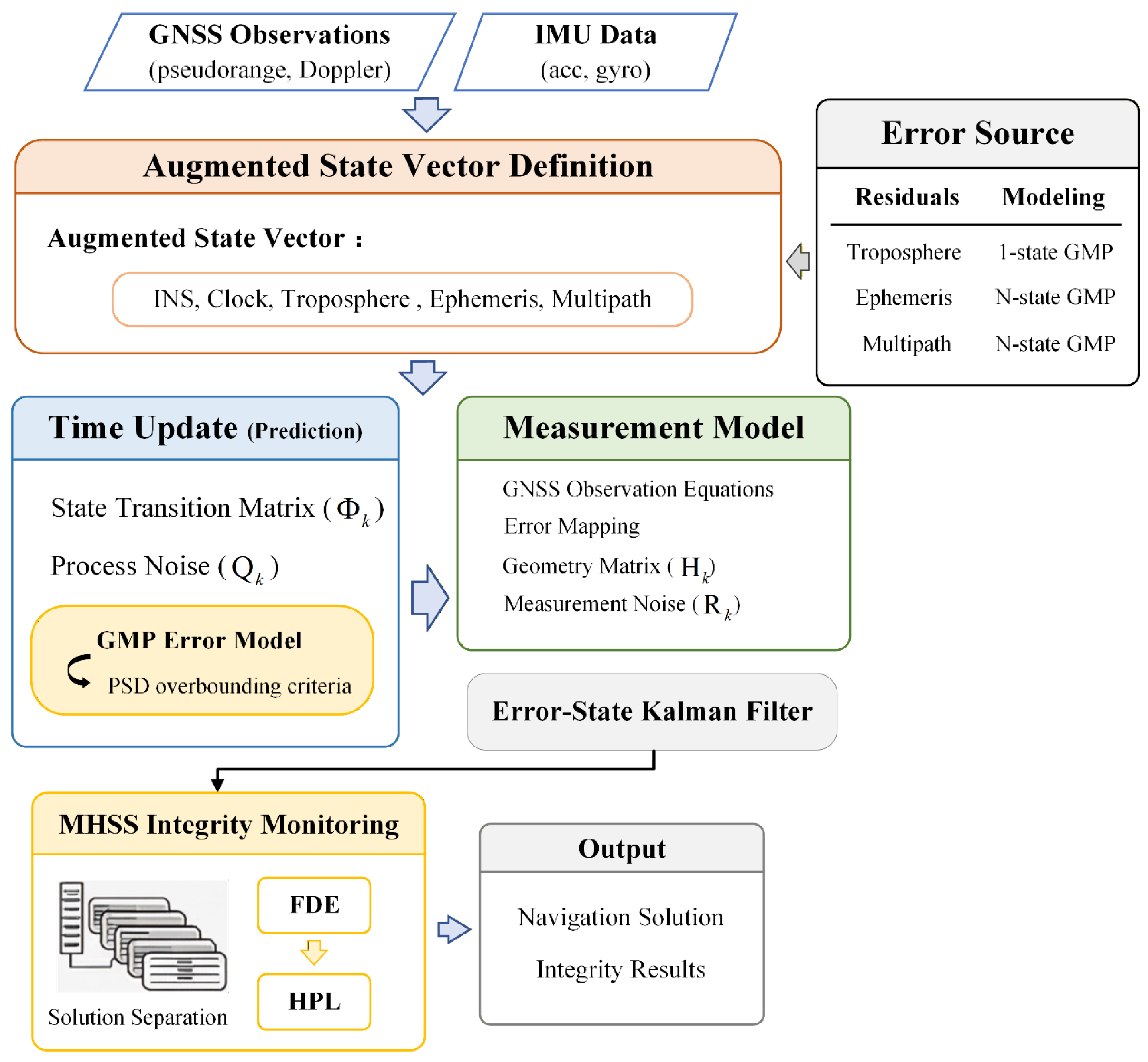
To achieve highly reliable integrity monitoring in complex urban environments, this paper proposes a tightly coupled GNSS/INS algorithm architecture based on physical error state augmentation. Targeting low-speed vehicular tightly coupled GNSS/INS positioning scenarios, this study focuses on the reliable bounding capability of positioning errors in urban obstructed environments. Unlike conventional navigation methods that primarily aim for high accuracy, this paper pays more attention to whether the filter covariance can reasonably reflect the actual uncertainty under complex observation conditions, thereby providing a reliable foundation for subsequent integrity monitoring. Positioning accuracy analysis is mainly used to verify that the proposed method, after introducing conservative error modeling, will not significantly degrade the basic navigation performance. The core evaluation metrics, however, include estimation consistency, protection level bounding capability, and system availability. The overall processing flowchart of the architecture is shown in Figure 1. The system first constructs an augmented state vector containing physical errors. During the time update phase, a first-order GMP is utilized as the system model to drive and predict the augmented states, and conservative parameter tuning is completed in combination with the frequency-domain overbounding criterion. During the measurement update phase, a measurement model with physical constraints is constructed to isolate external colored noise. Finally, the covariance output from the augmented filter bank, which guarantees consistency, is fed into the MHSS architecture to achieve FDE and rigorous protection level computation.

2.1. System Model

Accurately characterizing the composition and dynamic evolution of the system state is a crucial prerequisite for the Kalman filter to achieve reliable and consistent estimation. To this end, this section expands beyond the conventional formulation of purely navigational states and designs an augmented system model that incorporates physical errors from the external measurement domain.

2.1.1. Definition of the Augmented State Vector

The full error-state vector of the filter consists of two parts: the basic navigation states and the physically augmented states:

$$\delta x={\left[\begin{array}{cc}\delta x_{base}^T& \delta x_{aug}^T\end{array}\right]}^T$$

(1)

where $\delta x_{base}$ is the base navigation and clock error state, consisting of the 15-dimensional INS error state $\delta x_{INS}$ and the 2-dimensional receiver clock error state $\delta x_{clk}$. The INS error state $\delta x_{INS}$ adopts the classical 15-dimensional error state model to describe the error propagation of inertial sensors and mechanization, including attitude error $\delta \psi$, velocity error $\delta v$, position error $\delta r$, as well as accelerometer and gyroscope biases $b_a$ and $b_g$. The receiver clock error state $\delta x_{clk}$ includes the receiver equivalent clock bias $\delta t_u$ and clock drift $\delta {\dot{t}}_u$, which are used to compensate for the instability of the receiver crystal oscillator:

$$\delta x_{base}={\left[\begin{array}{cc}\delta x_{INS}^T& \delta x_{clk}^T\end{array}\right]}^T={\left[\begin{array}{ccccccc}\delta {\psi }^T& \delta v^T& \delta r^T& b_a^T& b_g^T& \delta t_u& \delta {\dot{t}}_u\end{array}\right]}^T$$

(2)

$\delta x_{aug}$ denotes the physically augmented states in the external measurement domain. To absorb colored noise, this study augments the states associated with three major physical error sources in complex urban dynamic environments. For the currently visible N satellites, the GNSS augmented error-state vector is constructed as:

$$\delta x_{aug}={\left[\begin{array}{ccc}\delta {\rho }_{trop}& \delta {\rho }_{eph}^T& \delta {\rho }_{mp}^T\end{array}\right]}^T$$

(3)

• Residual tropospheric zenith delay error $\delta {\rho }_{trop}$: After applying a conventional tropospheric model correction, part of the atmosphere-related error usually still remains in the observations. To distinguish the variation of the atmosphere itself from the effect caused by satellite geometry, the residual delay in the zenith direction is modeled as a common single augmented state.
• Residual ephemeris and satellite clock errors $\delta {\rho }_{eph}$: These errors mainly arise from systematic residuals in satellite orbit prediction and clock maintenance. Their physical evolution is extremely slow and is manifested as a long-correlation state with strong temporal correlation.
• Code multipath error $\delta {\rho }_{mp}$: In urban environments, the multipath effect caused by signal reflections is a major factor affecting positioning integrity. Unlike the previous two slowly varying errors, the variation frequency of multipath error is closely related to vehicle speed and the spatial distribution of surrounding buildings.

When constructing the physical augmented states, an N-dimensional state space is allocated for independent tracking of errors with strong spatial decorrelation, such as ephemeris and multipath errors, where N is the number of visible satellites. For residual tropospheric delay, considering the spatial consistency of local atmospheric conditions, a one-dimensional state variable is adopted, which is mapped to each observation channel through an elevation-angle projection function during the measurement update phase. Through this augmentation design, the filter is able to estimate and separate these colored noises, thereby preventing their impact on the navigation solution. It should be noted that the ionospheric delay is not modeled as an independent augmented state. The pseudorange observations used in this paper have already undergone ionospheric corrections during the standard GNSS preprocessing stage. Since the residual ionospheric error varies relatively slowly during the short-term vehicular experiments and is not a primary scenario-dependent error source in obstructed degraded environments, it is incorporated into the unmodeled observation error term for unified processing. Consequently, this paper focuses on explicitly modeling time-correlated errors such as residual ephemeris and clock errors, tropospheric delay, and code multipath.

2.1.2. First-Order Gauss-Markov Process and Parameter Tuning

A core premise of the standard Kalman filter is the assumption that the measurement noise is white noise; that is, the error at the current epoch is completely independent of the error at the next epoch. This holds true under ideal conditions, but in the actual complex environments of urban driving, physical errors such as multipath effects and atmospheric delays often exhibit persistence. If the filter ignores this temporal correlation and continues to treat them as white noise, it will misinterpret the persistent errors as valid observation information. This leads the filter to be overly optimistic about the accuracy of the state estimation, causing the computed posterior covariance matrix P to be smaller than the true error distribution. Consequently, the computed protection level shrinks significantly, ultimately posing a severe risk of missed alarms in complex environments.

To accurately describe the dynamic evolution process of the augmented states and resolve the measurement mismatch problem, considering that multipath and atmospheric residuals in urban environments exhibit continuity—manifesting as smooth attenuation or slow drift in the time series—this paper adopts a first-order Gauss-Markov process (GMP) to model the GNSS observation errors. The mathematical mechanism of this model aligns with the aforementioned time-varying patterns, enabling the transformation of external measurement noise into the evolution of internal system states within the filter. The discretized GMP state equation and the driving white noise variance are:

$$x_{k+1}=e^{-\frac{\mathsf{\Delta }t}{\tau }}·x_k+w_k,w_k\sim N(0,q_k)$$

(4)

$$q_k={\sigma }^2\left(1-e^{-\frac{2\mathsf{\Delta }t}{\tau }}\right)$$

(5)

where $\mathsf{\Delta }t$ is the system sampling interval; $\tau$ is the correlation time constant, ${\sigma }^2$ is the steady-state variance, and $w\left(t\right)$ is the driving white noise.

During the time-update stage of the error-state Kalman filter (ESKF), the error evolution is driven by the state transition matrix ${\mathsf{\Phi }}_k$ and the discrete process-noise covariance matrix $Q_k$. Since the INS errors, clock states, and GNSS augmented error states are mutually decoupled during prediction, ${\mathsf{\Phi }}_k$ takes a block-diagonal form:

$${\mathsf{\Phi }}_k=\left[\begin{array}{cc}{\mathsf{\Phi }}_{base}& 0\\ 0& {\mathsf{\Phi }}_{aug}\end{array}\right]$$

(6)

In the above equation, ${\mathsf{\Phi }}_{base}=\mathrm{diag}({\mathsf{\Phi }}_{INS},{\mathsf{\Phi }}_{clk})$. Here, ${\mathsf{\Phi }}_{INS}$ is the 15-dimensional inertial navigation error transition matrix, which describes the propagation of position, velocity, and attitude errors over time, as well as the effects of inertial sensor biases. To ensure the completeness of the system error estimation, its corresponding continuous-time system dynamic matrix $F_{INS}^e$ in the ECEF frame is constructed based on the classical INS mechanization error equations. Its matrix form is as follows:

$$F_{INS}^e=\left[\begin{array}{ccccc}-{\mathsf{\Omega }}_{ie}^e& 0_3& 0_3& 0_3& {\widehat{C}}_b^e\\ F_{21}^e& -2{\mathsf{\Omega }}_{ie}^e& F_{23}^e& {\widehat{C}}_b^e& 0_3\\ 0_3& I_3& 0_3& 0_3& 0_3\\ 0_3& 0_3& 0_3& 0_3& 0_3\\ 0_3& 0_3& 0_3& 0_3& 0_3\end{array}\right]$$

(7)

where ${\mathsf{\Omega }}_{ie}^e$ is the skew-symmetric matrix of the Earth’s rotation rate in the ECEF frame; ${\widehat{C}}_b^e$ is the direction cosine matrix from the body frame to the ECEF frame; and $F_{21}^e$ and $F_{23}^e$ are the state coupling terms induced by the specific force and the gravity field, respectively. Detailed derivations and expanded forms of the aforementioned basic INS error sub-matrices can be found in reference [24]. Considering the discrete-time implementation, the base state transition matrix can be obtained via a first-order approximation ${\mathsf{\Phi }}_{INS}\approx I+F_{INS}^e\mathsf{\Delta }t$. ${\mathsf{\Phi }}_{clk}$ is the clock-state transition matrix, given by:

$${\mathsf{\Phi }}_{clk}=\left[\begin{array}{cc}1& \mathsf{\Delta }t\\ 0& 1\end{array}\right]$$

(8)

${\mathsf{\Phi }}_{aug}$ is the transition matrix of the physically augmented error states and includes the GNSS error-model terms for all augmented states, including ephemeris/satellite clock errors, multipath, and tropospheric delay. Unlike the conventional framework, in order to properly mitigate the influence of colored noise during time update, each class of augmented error is modeled as a discrete first-order GMP, so that its state transition is represented by an exponential decay factor. The augmented-state transition matrix is constructed as:

$${\mathsf{\Phi }}_{aug}=\mathrm{diag}\left(e^{-\frac{\mathsf{\Delta }t}{{\tau }_{trop}}},e^{-\frac{\mathsf{\Delta }t}{{\tau }_{eph}}}{I}_N,e^{-\frac{\mathsf{\Delta }t}{{\tau }_{mp}}}{I}_N\right)$$

(9)

where $\mathsf{\Delta }t$ is the system sampling interval, $I_N$ is the N-dimensional identity matrix; and ${\tau }_{trop}$, ${\tau }_{eph}$, ${\tau }_{mp}$ denote the correlation time constants of the first-order GMP models corresponding to the three physical error sources.

The process-noise covariance matrix $Q_k$ also has a block-diagonal form:

$$Q_k=\left[\begin{array}{cc}{Q}_{base}& 0\\ 0& Q_{aug}\end{array}\right]$$

(10)

where $Q_{base}$ denotes the process noise of the basic navigation system and is projected into the basic state space through the noise-mapping matrix. The augmented part $Q_{aug}$ is based on direct physical modeling, and its corresponding noise-mapping matrix is the identity matrix I. The elements of $Q_{aug}$ are determined by the GMP steady-state variances, so as to ensure that the predicted covariance of the filter always overbounds the energy of the true physical errors:

$${\mathrm{Q}}_{aug}=\mathrm{diag}\left({\sigma }_{trpo}^2\left(1-e^{-\frac{2\mathsf{\Delta }t}{{\tau }_{trop}}}\right),{\sigma }_{eph}^2\left(1-e^{-\frac{2\mathsf{\Delta }t}{{\tau }_{eph}}}\right){\mathbf{1}}^{\mathrm{N}\times 1},{\sigma }_{mp}^2\left(1-e^{-\frac{2\mathsf{\Delta }t}{{\tau }_{mp}}}\right){\mathbf{1}}^{\mathrm{N}\times 1}\right)$$

(11)

To ensure the rigor of integrity monitoring, the selection of the aforementioned GMP parameters $(\tau ,{\sigma }^2)$ cannot rely on simple empirical fitting, but must adhere to the power spectral density (PSD) overbounding criterion. This criterion requires that the error model used for filter design must cover the energy distribution of the true error process in the frequency domain; that is, the PSD of the designed model must be no less than the PSD of the true error:

$$S_{model}\left(\omega \right)\ge S_{true}\left(\omega \right),\forall \omega \in [0,\infty )$$

(12)

For a discrete first-order GMP, its state transition coefficient can be expressed as:

$$\varphi =e^{-\mathsf{\Delta }t/\tau }$$

(13)

The corresponding theoretical PSD of this first-order GMP at frequency f can be written as:

$$S_{GMP}(f;\tau ,{\sigma }^2)={\displaystyle \frac{{\sigma }^2(1-{\varphi }^2)\mathsf{\Delta }t}{1+{\varphi }^2-2\varphi cos\left(2\pi f\mathsf{\Delta }t\right)}}$$

(14)

where $\mathsf{\Delta }t$ is the sampling interval, $\tau$ is the correlation time constant, and ${\sigma }^2$ is the steady-state variance. Equation (14) clearly reveals the impact of GMP parameters on the frequency-domain energy distribution: the correlation time $\tau$ primarily determines the concentration of error energy in the low-frequency region. A larger $\tau$ indicates a longer error duration and more pronounced low-frequency energy; meanwhile, the steady-state variance ${\sigma }^2$ determines the overall energy level of the error process. Under the condition of $\mathsf{\Delta }t\ll \tau$, the spectral intensity in the low-frequency band is approximately positively correlated with ${\sigma }^2\tau$, whereas the spectral intensity at the high-frequency end is mainly influenced by ${\sigma }^2/\tau$. Therefore, for time-correlated errors, conservative modeling is not equivalent to simply increasing all parameters simultaneously. Blindly inflating $\tau$ and ${\sigma }^2$ may yield a larger covariance bound, but it will also lead to a decrease in system availability.

From the perspective of integrity monitoring, the most dangerous errors in urban environments are not completely random high-frequency white noise, but rather the low-frequency persistent biases caused by multipath, NLOS propagation, and local blockages. According to the frequency-domain overbounding theory, if the augmented error model satisfies the PSD overbounding relationship in Equation (12), its corresponding autocovariance sequence can statistically cover the true error process, thereby providing a conservative input for the covariance propagation of the Kalman filter.

Based on the above analysis, rather than adopting a global parameter inflation approach, this paper employs a differentiated conservative parameter tuning strategy. For residual ephemeris and satellite clock errors, since satellite orbit and clock frequency errors are system-level slowly varying errors, their random variations typically only manifest over long time scales. Therefore, this paper models them as a long-correlation GMP, with the correlation time ${\tau }_{eph}$ set to the order of several hours to match their physical characteristics of slow evolution. The steady-state variance ${\sigma }_{eph}^2$ is conservatively set based on the statistical upper bound of the Signal-in-Space User Range Error (SIS-URE) defined in the GPS Standard Positioning Service (SPS) [25]. As for the residual tropospheric delay, because the local atmospheric state varies relatively slowly during short-term vehicular experiments, it is similarly modeled as a slowly varying common state in the zenith direction. A correlation time ${\tau }_{trop}$ on the order of tens of minutes and a correspondingly conservative steady-state variance ${\sigma }_{trop}^2$ are selected to cover the residual atmospheric uncertainty after model corrections.

Unlike the two types of slowly varying errors mentioned above, code multipath error is closely related to vehicle speed, building reflections, and satellite elevation angles, making it the most scenario-dependent time-correlated error source in urban environments. Regarding the correlation time ${\tau }_{mp}$, considering that vehicles may experience low-speed driving or brief stops in obstructed degraded segments, the multipath error often manifests as a quasi-static bias with a long duration. After selecting a correlation time ${\tau }_{mp}$ oriented toward the most severe persistent conditions, the multipath steady-state variance ${\sigma }_{mp}^2$ is further determined based on the PSD overbounding criterion. Specifically, the variance is selected such that the theoretical PSD of the first-order GMP covers the empirical PSD of the multipath-dominated pseudorange residuals in the urban degraded segment:

$$S_{GMP}(f;{\tau }_{mp},{\sigma }_{mp}^2)\ge {\widehat{S}}_{res}\left(f\right),f\in \mathsf{\Omega }$$

(15)

where ${\widehat{S}}_{res}\left(f\right)$ is the empirical PSD estimated from the pseudorange residuals in the urban degraded segment, and $\mathsf{\Omega }$ represents the main low-frequency range dominated by colored errors. In this way, the conservative model primarily enhances the overbounding capability against low-frequency persistent errors, rather than indiscriminately inflating the measurement noise across the entire frequency band. Therefore, the parameter tuning method adopted in this paper can guarantee the integrity safety bound while avoiding the unnecessary enlargement of the protection level caused by over-conservatism, thus achieving a reasonable trade-off between safety and availability. The specific empirical PSD estimation process for multipath and the selection results of the conservative variance will be further detailed in Section 3.2.

2.2. Measurement Model

When GNSS pseudorange and pseudorange-rate observations are available, the filter enters the measurement-update stage. The measurement vector $\delta z_k$ is formed by subtracting the line-of-sight range and relative velocity predicted by the INS from the actual GNSS pseudorange and pseudorange-rate observations:

$$\delta z_k=\left[\begin{array}{c}\delta z_{\rho }\\ \delta z_{\dot{\rho }}\end{array}\right]=\left[\begin{array}{c}{\rho }_{GNSS}-{\rho }_{INS}\\ {\dot{\rho }}_{GNSS}-{\dot{\rho }}_{INS}\end{array}\right]$$

(16)

To map the full error-state vector into the observation domain, the measurement Jacobian matrix $H_k$ must be strictly consistent with the block structure of the state vector. In this paper, it is decomposed into two parts: the basic navigation mapping and the physically augmented constraint mapping:

$$H_k=\left[\begin{array}{cccccc}{H}_{pos}& {\mathbf{1}}_{N\times 1}& {\mathbf{0}}_{N\times 1}& M_{trop}& I_{N\times N}& I_{N\times N}\\ H_{vel}& {\mathbf{0}}_{N\times 1}& {\mathbf{1}}_{N\times 1}& {\mathbf{0}}_{N\times 1}& {\mathbf{0}}_{N\times N}& {\mathbf{0}}_{N\times N}\end{array}\right]$$

(17)

In the above equation, the first three block columns constitute the basic navigation mapping. $H_{pos}$ and $H_{vel}$ are the geometry matrices, which respectively reflect the influence of position error on pseudorange and velocity error on pseudorange rate. The second and third block columns map the effects of receiver clock bias and clock drift on the observations.

The last three block columns form the augmented constraint mapping and explicitly establish the relationship between each satellite observation channel and the external physical errors. $I_N$ is the N-dimensional identity matrix and corresponds to the residual ephemeris error and code multipath error, respectively. Since these two physical errors are highly independent across satellite channels, they can be directly added to the pseudorange observation equation. $M_{trop}=\mathrm{diag}{(m\left(E{l}_1\right),\dots ,m\left(E{l}_N\right))}^T$ is the tropospheric projection function, which maps the common zenith-delay state to the corresponding line-of-sight direction according to the elevation angle of each satellite channel. Because the pseudorange-rate observations are only weakly affected by the above slowly varying physical errors, the augmented mapping terms in the lower half of the measurement matrix are all set to zero.

The observation-noise covariance matrix $R_k$ only needs to describe the intensity of the unmodeled Gaussian white noise:

$$R_k=\mathrm{diag}({\sigma }_{\rho ,1}^2,\dots ,{\sigma }_{\rho ,N}^2,{\sigma }_{\dot{\rho },1}^2,\dots ,{\sigma }_{\dot{\rho },N}^2)$$

(18)

where ${\sigma }_{\rho ,i}^2$ and ${\sigma }_{\dot{\rho },i}^2$ denote the measurement-noise variances of the pseudorange and pseudorange rate of the i-th satellite, respectively.

2.3. Multiple Hypothesis Solution Separation Based on Augmented Covariance

To achieve real-time GNSS fault detection and protection level computation, this paper introduces the augmented filter bank designed in Section 2.2 into the multiple hypothesis solution separation (MHSS) architecture. This paper retains the solution separation detection logic and protection level computation formulation of the standard MHSS, with the difference lying in the construction method of the underlying filter covariance matrix. In urban obstructed environments, traditional filters adopt the Gaussian white noise assumption, which easily underestimates state uncertainty by neglecting time-correlated errors, thereby resulting in underestimated detection thresholds and horizontal protection levels. In contrast, this paper employs the covariance matrix output by the physical-error-augmented filter and combines it with the PSD overbounding criterion for parameter tuning. This establishes the MHSS detection thresholds and protection level computations on a more consistent covariance foundation.

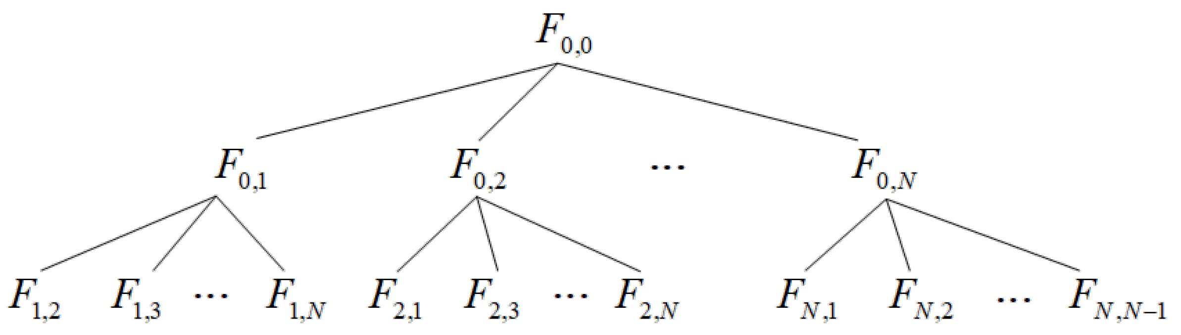
As shown in Figure 2, the MHSS architecture consists of a main filter that utilizes all N visible satellites, running in parallel with N sub-filters that each exclude the observation data of the m-th satellite. In the figure, $F_{0,0}$ represents the global main filter containing all visible satellites; the first-tier $F_{0,m}$ represents the sub-filter excluding the observation data of the m-th satellite, which is used for fault detection; the second-tier $F_{m,n}$ represents the sub-sub-filter that further excludes the n-th satellite on top of excluding the m-th satellite, which is used for the fault identification and isolation stage. Both the main filter and the sub-filters employ the augmented state vector and process noise model to ensure that every solution branch possesses the capability to handle colored noise.

When a fault occurs on a certain satellite, the main-filter solution containing that satellite will deviate, whereas the sub-filter solution excluding the faulty satellite will remain unaffected. Therefore, fault identification can be achieved by monitoring the consistency between the full-set solution and the subset solutions. The separation vector and its corresponding covariance matrix are defined as:

$$\mathsf{\Delta }{x}_{0m}={\widehat{x}}_0-{\widehat{x}}_m$$

(19)

$$\mathsf{\Delta }{P}_{0m}=P_m-P_0$$

(20)

where ${\widehat{x}}_0$ and $P_0$ denote the horizontal position estimate and posterior covariance matrix of the main filter, respectively, and ${\widehat{x}}_m$ and $P_m$ are the corresponding outputs of the m-th sub-filter. Since horizontal positioning performance is of primary concern in vehicular navigation scenarios, the horizontal position component $\mathsf{\Delta }{x}_{0m}^{hpos}$ and its corresponding covariance matrix $\mathsf{\Delta }{P}_{0m}^{hpos}$ are extracted in the actual computation. An eigenvalue decomposition is then performed in the horizontal plane:

$$\mathsf{\Delta }{P}_{0m}^{hpos}=V\mathsf{\Lambda }{V}^T$$

(21)

$$d{X}^{hpos}=V^T·\mathsf{\Delta }{x}_{0m}^{hpos}$$

(22)

where $\mathsf{\Lambda }$ and V denote the eigenvalue matrix and the corresponding eigenvector matrix, respectively. From this decomposition, two eigenvalues of $\mathsf{\Delta }{P}_{0m}$ are obtained, and the larger eigenvalue indicates the larger error variance. Assuming that the maximum eigenvalue ${\lambda }_{max}$ is the i-th element, the test statistic $d_{0m}$ is defined as the element of $d{X}^{hpos}$ corresponding to this maximum eigenvalue:

$$d_{0m}=\left|d{X}^{hpos}\left(i\right)\right|$$

(23)

The detection threshold $T_{0m}$ for the m-th sub-filter is determined based on the target false alarm probability $P_{FA}$. By uniformly allocating $P_{FA}$ among the total of N satellites, the detection threshold is given by:

$$T_{0m}=\sqrt{{\lambda }_{max}}·Q^{-1}\left({\displaystyle \frac{P_{FA}}{2N}}\right)$$

(24)

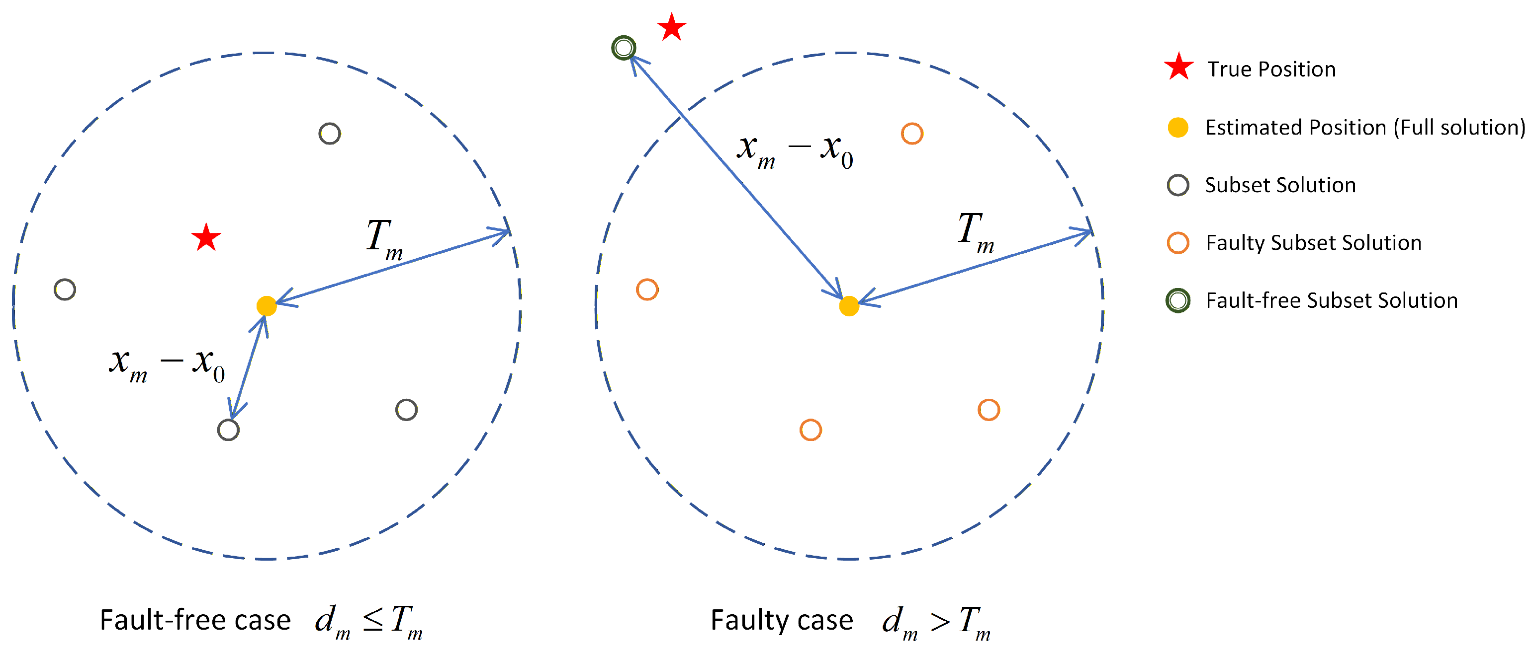
where $Q^{-1}(·)$ is the inverse tail-probability function of the standard normal distribution. If there exists any subset such that $d_{0m}>T_{0m}$, the system is declared faulty, and the satellite causing the largest statistical deviation is excluded. The principle of the fault exclusion algorithm is illustrated in Figure 3.

The protection level (PL) is the final output of integrity monitoring. It is defined as the upper bound of the position error that the system can guarantee under a prescribed integrity risk probability. Based on the worst-case logic of MHSS, the horizontal protection level (HPL) is determined by the maximum positioning error that may be induced under all subset hypotheses:

$$HPL={\displaystyle \underset{m=1}{\overset{N}{max}}}\left(HP{L}_m\right)$$

(25)

For each subset hypothesis, its protection level $HP{L}_m$ is jointly determined by the detection threshold and the uncertainty of the subset solution:

$$HP{L}_m=T_{0m}+{\sigma }_m·Q^{-1}\left(P_{md}\right)$$

(26)

where ${\sigma }_m$ is the maximum estimated error standard deviation of the m-th subset filter in the horizontal direction.

The analytical derivations of the detection threshold $T_{0m}$ and the protection level follow the standard multiple hypothesis solution separation theoretical framework and can be found in reference [22,23]. As shown in Equations (24) and (26), both the detection threshold and the protection level are mathematically in strict positive correlation with the eigenvalue ${\lambda }_{max}$ or standard deviation ${\sigma }_m$ extracted from the covariance matrix. If the underlying filter falls into an “over-confident” state due to unmodeled colored noise, it will directly cause the calculated $T_{0m}$ and $HPL$ to shrink simultaneously, making the system lose its overbounding capability when facing hazardous errors.

Therefore, the covariance matrix in the MHSS architecture of this paper no longer directly employs the covariance output by the traditional white noise KF, but is instead provided by the filter containing the physical error augmented states. Because the augmented filter introduces the uncertainties of time-correlated errors such as multipath and residual tropospheric delay during the time update phase, its output matrix can provide a more consistent variance baseline for the solution separation statistics, detection thresholds, and HPL computations. In this way, in the presence of obstructed degradation and slowly varying pseudorange biases, the MHSS can compute the protection level based on a more conservative covariance bound, thereby reducing the risk of the HPL underestimating the true horizontal error.

3. Experimental Results and Analysis

3.1. Experimental Data and Observation Conditions

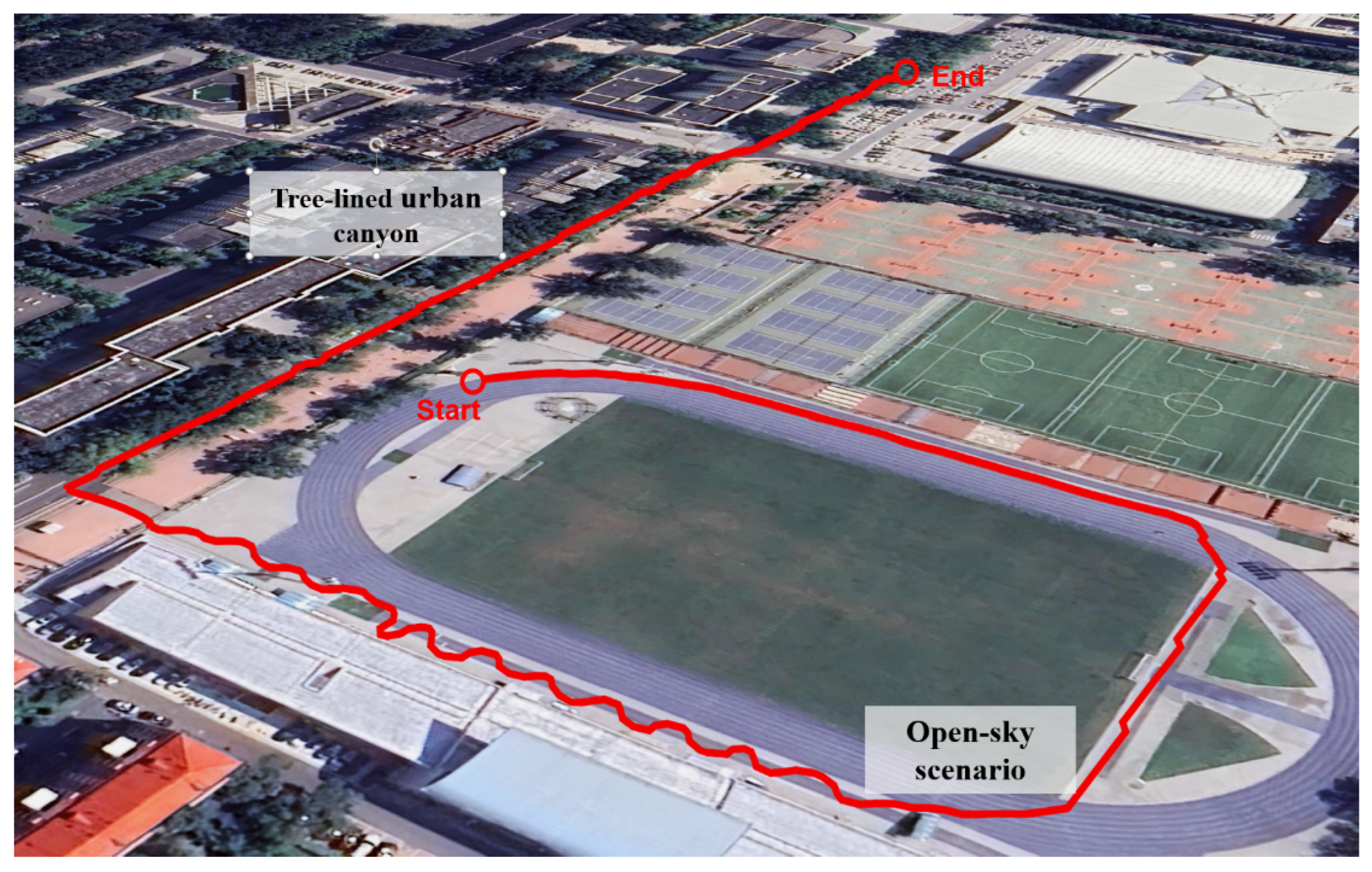
To verify the effectiveness of the state augmentation model and the conservative overbounding parameter tuning strategy proposed in this paper within a real physical environment, the BUAA open-source vehicular GNSS/INS field test dataset was selected for evaluation, which was collected in a typical high-dynamic semi-urban/campus complex section. The experimental data were collected from a multi-sensor data acquisition platform mounted on a test vehicle. The specific hardware and software configuration information for this experiment is shown in

Table 1. Hardware/Software configuration of the experimental platform.

Category	Equipment	Specifications
GNSS Receiver	NovAtel ProPak6	Outputs raw measurements including pseudorange, pseudorange rate, Doppler, and signal strength.
IMU	NovAtel SPAN-IGM-S1	Outputs three-axis specific force and angular rate measurements in the body frame (FRD).
Reference Ground Truth	NovAtel Waypoint Inertial Explorer	Commercial post-processing software; uses RTK/INS tightly coupled forward-backward smoothing to ensure absolute reliability.

. The reference trajectory used for error statistics and NEES computation was obtained through post-processing with NovAtel Waypoint Inertial Explorer. This software generates reference positions based on tightly coupled RTK/INS forward-backward smoothing solutions, and it is used in this paper as the reference ground truth for evaluating positioning errors and state consistency within the experimental segment. A schematic diagram of the test vehicle’s driving trajectory is shown in Figure 4.

The total duration of the intercepted test data is approximately 450 s, which encompasses a continuous process of observation environment changes. From approximately 0 to 200 s of the experiment, the vehicle traveled in a relatively open area with a good GNSS observation geometry, and the measurement errors were mainly affected by long-correlation slowly varying errors such as ephemeris and tropospheric residuals. It should be noted that the wavy trajectory corresponds to low-speed turning maneuvers performed by the test vehicle along a pre-planned route, which can provide a certain dynamic excitation for the tightly coupled state estimation. After approximately 200 s of the experiment, the vehicle entered an area with tree-lined avenues and buildings, where GNSS signals began to be affected by blockage, NLOS propagation, and multipath reflections, resulting in degraded observation conditions.

Table 2. Environmental and observation condition statistics of the experimental segments.

Segment Description	Main Observation Characteristics	Number of Satellites Used in Positioning	PDOP Range
Open-sky area (approximately 0–200 s)	Stable satellite geometry	14.6 (12–15)	0.8–1.2
Tree-lined/building-obstructed area (approximately 200–450 s)	Increased blockage, multipath, and NLOS effects	11.4 (8–13)	1.5–2.8

presents the statistics of observation conditions in the different segments.

In the open area from 0 to 200 s, the number of satellites used in the positioning solution mostly remained at 15, dropping to 12–14 at localized moments; the position dilution of precision (PDOP) stayed around 0.8–1.2, indicating that the satellite geometry was relatively stable during this phase. After entering the obstructed degraded segment at approximately 200 s, the number of satellites used in the solution decreased to 8–13, and the PDOP concurrently rose to approximately 1.5–2.8, indicating a degradation in both satellite availability and geometry.

To verify the impact of different error modeling assumptions on the subsequent estimation consistency and integrity monitoring results, this paper establishes three comparative schemes:

(1)

Standard tightly coupled Kalman filter (Standard KF), serving as the conventional baseline scheme. This scheme does not consider the temporal correlation of GNSS observation errors, and the measurement noise is modeled solely as Gaussian white noise.

(2)

Augmented KF with typical parameters (Augmented-Typical), which introduces a first-order GMP physical error augmented state into the filter. Its correlation time and steady-state variance adopt conventional empirical parameters to represent the nominal error level in open or weakly degraded environments.

(3)

Augmented KF with conservative parameters (Augmented-Conservative), which similarly employs the physical error augmented model, but further conducts conservative parameter tuning for key colored error sources based on the frequency-domain PSD overbounding criterion. This enables the covariance output by the filter to more reliably cover the time-correlated errors in complex urban environments.

The experiment in this paper is conducted based on a segment of real-world vehicular data in a campus/semi-urban scenario. This route includes both an open area and a tree-lined/building-obstructed area, serving as a representative case study to verify the effectiveness of the proposed method in typical observation-degraded scenarios. Future work still needs to incorporate more routes, different urban canyon geometries, and varying satellite visibility conditions to further validate the generalization capability of the method.

3.2. GMP Parameter Determination and PSD Overbounding Validation

To provide a unified parameter foundation for the subsequent augmented filtering experiments, this paper establishes two sets of GMP parameters: a typical parameter model and a conservative parameter model. The typical parameter model adopts conventional empirical values to represent the nominal error level in open or lightly degraded environments, serving as a non-conservative control. The conservative parameter model, on the other hand, is oriented toward the obstructed degraded scenario in this experiment—namely, the observation conditions characterized by enhanced multipath, exacerbated blockage, and reduced satellite visibility after the vehicle enters the tree-lined avenues and dense building areas at approximately 200 s. This model is used to provide a more reliable covariance baseline for integrity monitoring.

In the conservative parameter model, residual ephemeris and satellite clock errors, as well as residual tropospheric delay, are all treated as slowly varying background error terms. The former belongs to satellite-system-level slowly varying errors, while the latter belongs to local atmospheric slowly varying common errors. Both have long variation time scales and are difficult to estimate independently and reliably from the residuals of a single short-term vehicular experiment. Therefore, this paper does not perform data-driven PSD estimation for these two types of errors, but instead adopts fixed conservative background parameters to provide a slowly varying uncertainty baseline for the filter.

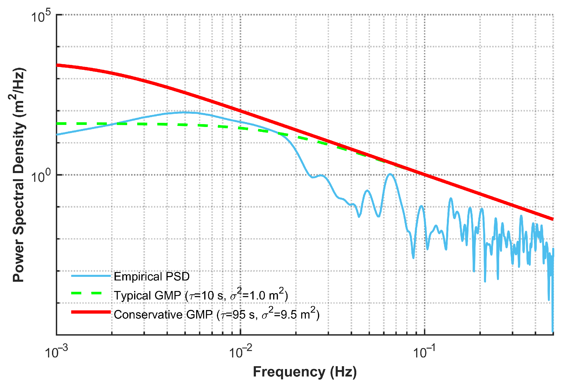
Code multipath error is the most scenario-dependent time-correlated error source in urban degraded environments. To avoid underbounding caused by relying solely on empirical variance settings, this paper further validates the conservative multipath parameters by comparing the empirical PSD with the theoretical GMP PSD. In the multipath GMP model, the correlation time ${\tau }_{mp}$ primarily determines the attenuation shape of the theoretical PSD curve in the low-frequency band, while the steady-state variance ${\sigma }_{mp}^2$ primarily determines the overall amplitude of the spectral line. Considering that vehicles may experience low-speed driving or brief stops in obstructed degraded segments, the multipath error often manifests as a quasi-static bias with a long duration. To cover such low-frequency persistent errors, this paper first fixes ${\tau }_{mp}$ at 95 s as the conservative correlation time scale for the persistent biases in this obstructed degraded segment. On this basis, the empirical PSD is estimated using the pseudorange residuals of satellites that are significantly affected by blockage and multipath in the obstructed degraded segment. These residuals are obtained from the raw pseudorange observations after applying standard corrections for satellite clock errors and tropospheric delays. In this obstructed degraded segment, their low-frequency variations are primarily driven by signal blockage, NLOS propagation, and multipath reflections; therefore, they are used to represent the multipath-dominated time-correlated errors. The extracted empirical PSD aims to reflect the multipath-related background error level under this scenario and is used to verify the effectiveness of the parameter tuning method. In specific implementation, the residual sequence is first demeaned, and then the power spectral density is estimated using Welch’s method. Subsequently, by adjusting ${\sigma }_{mp}^2$ and selecting a conservative variance capable of covering the low-frequency peaks of the empirical PSD, ${\sigma }_{mp}^2$ is ultimately determined to be 9.5 ${\mathrm{m}}^2$.

Figure 5 presents the empirical PSD curve of the pseudorange residuals in the obstructed degraded segment of this experiment, along with the theoretical PSDs of the first-order GMP corresponding to the typical model and the conservative model. The blue curve in the figure is calculated from representative satellite pseudorange residuals in the obstructed degraded segment after approximately 200 s in this experiment. In this segment, the vehicle enters tree-lined avenues and dense building areas, where satellite signals are more susceptible to blockage, NLOS propagation, and multipath reflections, causing some pseudorange residuals to exhibit relatively obvious low-frequency persistent bias characteristics. Therefore, these residuals are treated as a representative sample of multipath-related colored errors in the obstructed degraded environment, rather than being viewed as completely isolated single multipath errors. It can be seen that in the low-frequency region with enhanced blockage and multipath, the empirical PSD curve exceeds the typical model curve, indicating that the typical parameters underestimate the low-frequency energy of the persistent multipath biases in this segment. In contrast, the conservative model can effectively overbound the low-frequency portion of the empirical PSD. At the same time, in the high-frequency region, the PSD curves of the typical model and the conservative model are close to each other because the two sets of parameters have similar ${\sigma }^2/\tau$ ratios. This phenomenon indicates that the conservative model does not simply inflate the noise across the entire frequency band, but primarily enhances the overbounding capability against low-frequency time-correlated errors. Therefore, while improving the integrity safety margin, this parameter set can avoid the unnecessary enlargement of the protection level caused by over-conservatism. The specific parameter configurations of the two augmented models are detailed in

Table 3. GMP model parameter configurations.

Error Component	Parameter	Typical Model	Conservative Model
Ephemeris & Clock	$\tau$	4 h	14.1 h
	${\sigma }^2$	1.56 ${\mathrm{m}}^2$	3.5 ${\mathrm{m}}^2$
Residual Troposphere	$\tau$	900 s	$1.56\times {10}^3$ s
	${\sigma }^2$	0.014 ${\mathrm{m}}^2$	0.025 ${\mathrm{m}}^2$
Code Multipath	$\tau$	10 s	95 s
	${\sigma }^2$	1.0 ${\mathrm{m}}^2$	9.5 ${\mathrm{m}}^2$

.

3.3. Positioning Performance Analysis

Before evaluating system-level integrity, it is necessary to first examine the impact of different error modeling strategies on the positioning accuracy of the basic navigation solution. The purpose of this section is not to claim that the proposed method mainly contributes to positioning accuracy improvement, but to verify whether the system’s positioning accuracy remains at a reasonable level after introducing the error overbounding parameters. Traditional integrity enhancement methods often bound unmodeled errors by directly inflating the measurement noise variance. Although this approach may increase the safety margin, it easily leads to a decline in positioning accuracy and continuity. By contrast, this paper adopts the physical error augmented model, introducing time-correlated errors into the filter states for estimation and absorption. Its objective is to achieve safer integrity overbounding without affecting the system’s basic positioning function.

The positioning error comparison and detailed accuracy statistical metrics of the three models in the open-sky scenario during the first 200 s of the experimental segment are shown in

Table 4. Positioning accuracy statistics comparison in the open-sky segment.

Metric	Standard KF	Augmented KF (Typical)	Augmented KF (Conservative)
North Error (m)	0.405	0.292	0.314
East Error (m)	0.326	0.212	0.280
Down Error (m)	0.657	0.542	0.487
Horizontal RMS (m)	0.520	0.361	0.421
3D Position RMS (m)	0.838	0.644	0.651

:

Analyzing the results of the open-sky segment in Table 4, it can be seen that the GNSS signal quality is good at this time, and colored noises such as multipath are not significant. Therefore, the Augmented-Typical model based on nominal parameters matches the current observation conditions better, achieving the best positioning accuracy (3D RMS of 0.644 m). In contrast, because the Augmented-Conservative model introduces more conservative process noise and error correlation times, it appropriately reduces the reliance on GNSS observations during the filtering process, resulting in a slight decrease in positioning accuracy compared to the Augmented-Typical model. However, the magnitude of the decrease is small, indicating that the conservative parameters do not cause noticeable accuracy loss in the open-sky environment. Additionally, the positioning results of both augmented models are superior to those of the Standard KF (0.838 m), which does not consider time-correlated errors. This demonstrates that the physical error augmented states can provide compensation for residual slowly varying errors and weak colored errors without degrading the basic navigation performance.

After approximately 200 s, the vehicle enters tree-lined avenues and dense building areas. Satellite signals are affected by blockage, NLOS propagation, and multipath reflections, leading to degraded observation conditions. The positioning accuracy statistical metrics of the three models in this segment are shown in

Table 5. Positioning accuracy statistics comparison in the blocked segment.

Metric	Standard KF	Augmented KF (Typical)	Augmented KF (Conservative)
North Error (m)	0.902	0.873	0.779
East Error (m)	0.494	0.279	0.334
Down Error (m)	1.454	0.502	0.629
Horizontal RMS (m)	1.029	0.917	0.848
3D Position RMS (m)	1.781	1.045	1.056

:

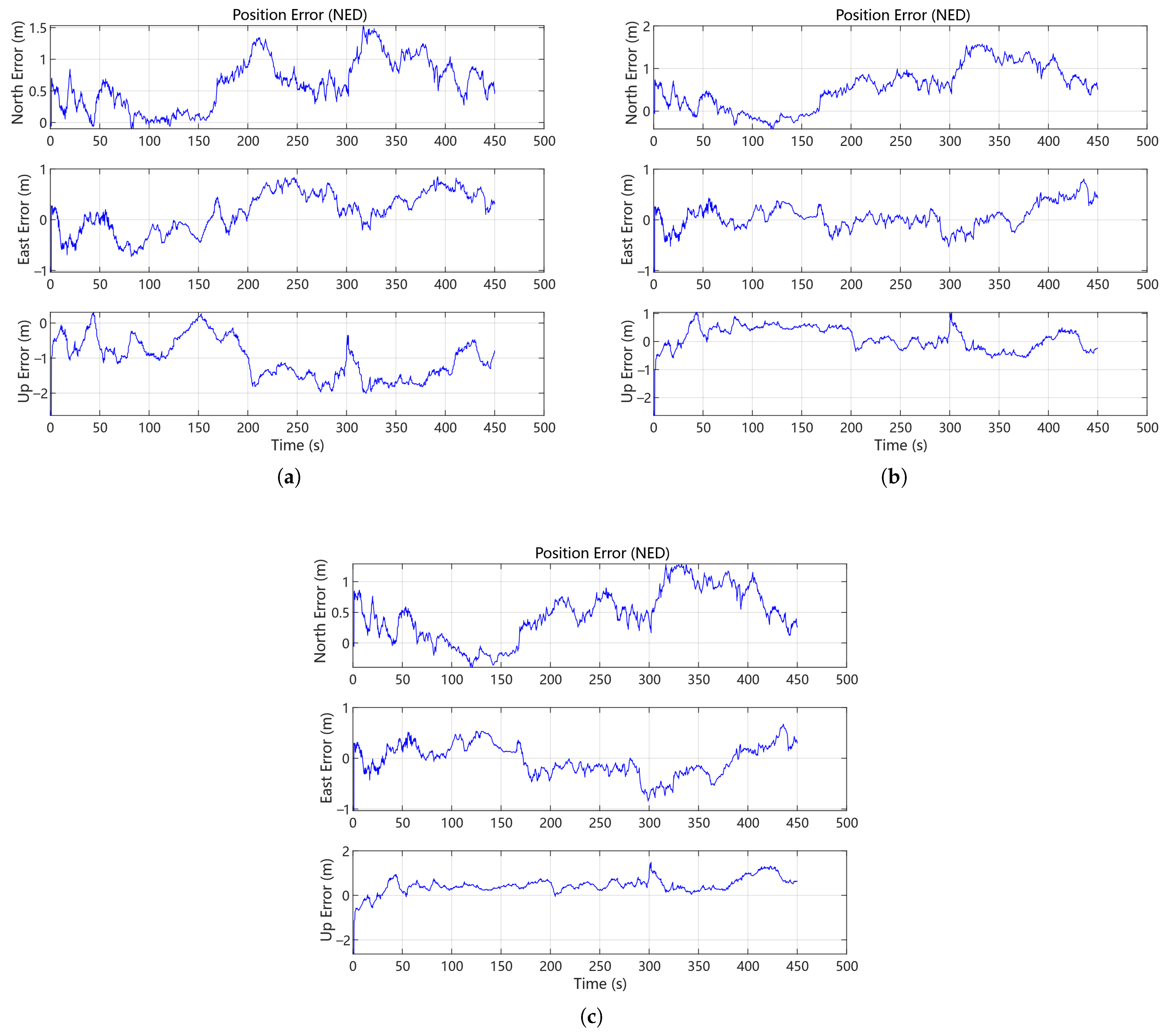
As shown in Table 5, the error of the Standard KF model increases significantly in this segment, with the 3D RMS reaching 1.781 m, where the growth of the vertical error is particularly pronounced. This is because blockage, multipath, and residual atmospheric errors exhibit stronger temporal correlation in this segment, whereas the Standard KF still adopts the independent white noise assumption, making it prone to placing excessive confidence in low-quality GNSS observations. In contrast, by introducing GMP error states, the two augmented models possess a stronger capability to absorb persistent observation biases, reducing their 3D RMS to 1.045 m and 1.056 m, respectively. Further comparison between the two augmented models reveals that, although the Augmented-Conservative model employs more conservative correlation times and steady-state variances, it does not experience noticeable positioning accuracy degradation in this obstructed degraded segment. Its 3D RMS is basically comparable to that of the Augmented-Typical model, while its horizontal RMS decreases from 0.917 m to 0.848 m. This indicates that the conservative parameters do not simply sacrifice positioning accuracy in exchange for a safety bound; in this obstructed degraded segment, the conservative GMP parameters can more reasonably describe low-frequency time-correlated errors, thereby providing a more reliable covariance foundation for subsequent integrity overbounding while maintaining basic positioning performance. To fully present the overall performance of the different models across the entire experimental trajectory, the time series of positioning errors for the three models are shown in Figure 6, and the overall positioning accuracy statistics are listed in

Table 6. Positioning accuracy statistics comparison over the whole trajectory.

Metric	Standard KF	Augmented KF (Typical)	Augmented KF (Conservative)
North Error (m)	0.725	0.751	0.618
East Error (m)	0.428	0.252	0.311
Down Error (m)	1.169	0.425	0.570
Horizontal RMS (m)	0.841	0.792	0.692
3D Position RMS (m)	1.440	0.899	0.896

:

As seen from Table 6, the 3D positioning errors of both augmented models are lower than that of the Standard KF over the entire experimental route. Specifically, the 3D positioning RMS of the augmented model using typical parameters (Augmented-Typical) drops from 1.440 m to 0.899 m, and the augmented model using conservative parameters (Augmented-Conservative) further maintains a similar level of 0.896 m. This demonstrates that after explicitly modeling time-correlated errors as augmented states, the filter can more effectively absorb persistent observation biases in obstructed and multipath environments. Because the Standard KF relies on the Gaussian white noise assumption, it struggles to characterize such colored errors and is therefore more susceptible to estimation deviations after the vehicle enters the obstructed degraded segment. The improvement of the two augmented models in the vertical direction is relatively obvious, which is consistent with the characteristic that the vertical direction is usually more sensitive to satellite geometry variations and residual tropospheric errors, further validating the necessity of introducing physical error augmented modeling.

Further comparison of the two augmented models shows that the positioning accuracy of the error-augmented model with conservative parameters is basically comparable to that of the typical model. This indicates that the introduction of conservative parameters does not cause obvious loss in positioning accuracy. On the contrary, throughout the entire trajectory involving blockage and multipath effects, the Augmented-Conservative model characterizes low-frequency time-correlated errors more robustly. Therefore, it can maintain basic navigation accuracy while providing a more reliable covariance baseline for subsequent integrity assessment.

3.4. Estimation Consistency Analysis

The effectiveness of integrity monitoring algorithms such as MHSS is founded on the premise that the covariance matrix P can truly reflect the state estimation uncertainty. To directly verify with data whether the physical error augmented model and its conservative parameter settings proposed in this paper can reasonably represent actual error uncertainty in complex environments, the Normalized Estimation Error Squared (NEES) is introduced as an evaluation metric. NEES is defined as the weighted norm of the true error vector with respect to the covariance matrix, calculated as follows:

$${ϵ}_k={(x_k-{\widehat{x}}_k)}^T{P}_k^{-1}(x_k-{\widehat{x}}_k)$$

(27)

where $(x_k-{\widehat{x}}_k)$ denotes the true position error vector, and $P_k$ is the position covariance matrix output by the filter.

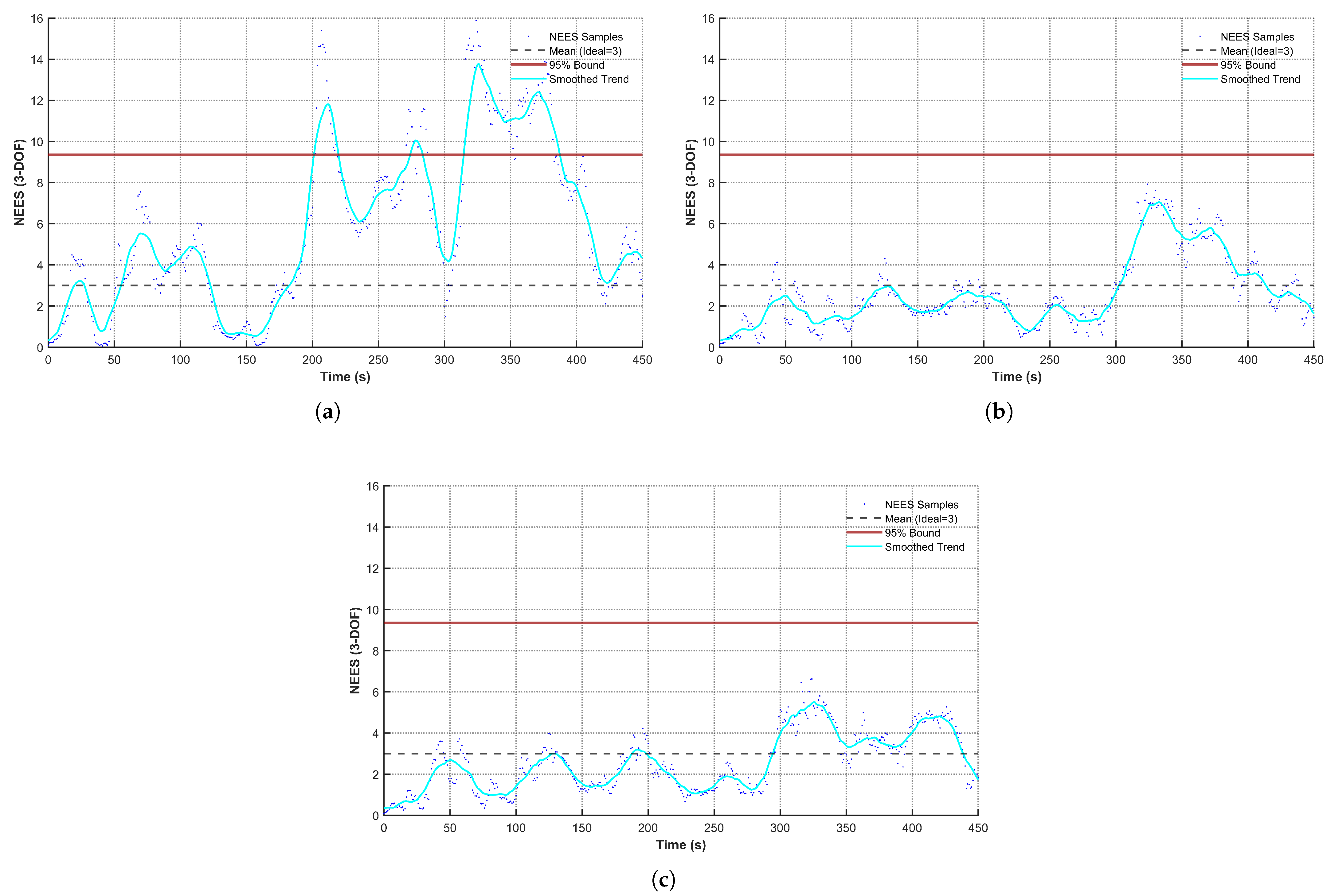
Theoretically, the NEES of a 3D position estimation should follow a chi-square distribution with 3 degrees of freedom (DOF). If the NEES exceeds the upper bound of the confidence interval, it indicates that the matrix estimated by the filter fails to cover the true physical errors. This will cause the protection level computed by the algorithm to be too small, thereby inducing integrity risks. Figure 7 illustrates the time series variations of position estimation consistency for the three different models. The red solid line in the figure represents the 95% confidence upper bound (approximately 9.35), and the black dashed line represents the theoretical mean (3.0).

As shown in Figure 7a, the NEES curve of the Standard KF remains within a reasonable range in the open-sky segment from 0 to 200 s. However, after the vehicle enters the obstructed degraded segment, with the decline in observation quality and the enhancement of time-correlated errors, the NEES rises rapidly and maintains a high level between 200 and 400 s. This result indicates that the Standard KF model experiences covariance underestimation under the influence of colored noise, and its output P matrix fails to cover the actually increased physical errors. Therefore, if the protection level is computed directly based on this covariance matrix, there will be a risk of an overly small protection level and integrity overbounding failure.

Comparing Figure 7b,c, it can be seen that neither of the result curves using the error-augmented models breaches the confidence upper bound, indicating that physical error modeling can improve the consistency of the filter. In Figure 7b, the NEES of the Typical model remains near the theoretical mean for most of the time, exhibiting good consistency. However, a noticeable elevation appears around 300 s, indicating that the overbounding safety margin of the nominal parameters is relatively limited in scenarios with enhanced blockage and multipath. In contrast, because the Conservative model in Figure 7c adopts more conservative GMP parameters, its covariance matrix can provide a more reliable uncertainty boundary for persistent colored errors. Consequently, its NEES peak at 300 s is lower, demonstrating that it possesses stronger estimation consistency and robustness in complex observation environments.

It should be noted that after approximately 400 s, the NEES of the Standard KF and the Typical model shows a downward trend, whereas the NEES of the Conservative model exhibits a short-term upward trend. This is primarily related to how different models respond to persistent errors in the obstructed segment. As the vehicle gradually leaves the strongly obstructed area, the instantaneous positioning errors of the Standard KF and the Typical model decrease, causing their NEES to fall back accordingly. Meanwhile, because the Conservative model employs a multipath augmented state with a longer correlation time, it retains a stronger temporal memory of the persistent biases from the previous stage. Its state and covariance adjustments experience a certain lag, which may cause a short-term rise in NEES. Since this process never breaches the confidence upper bound, it indicates that the estimation consistency of the Conservative model is not compromised.

3.5. Protection Level Overbounding and Integrity Statistical Analysis

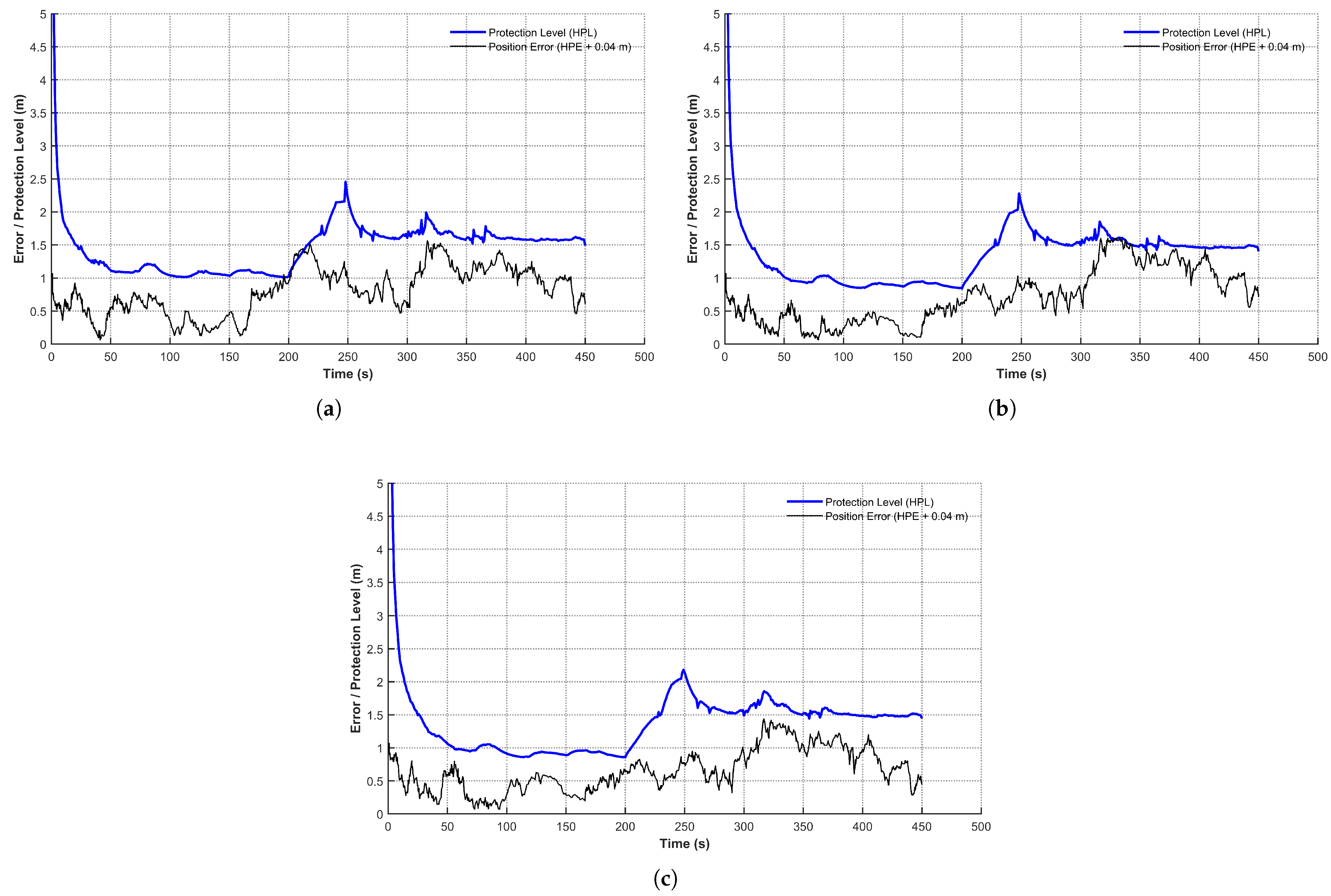
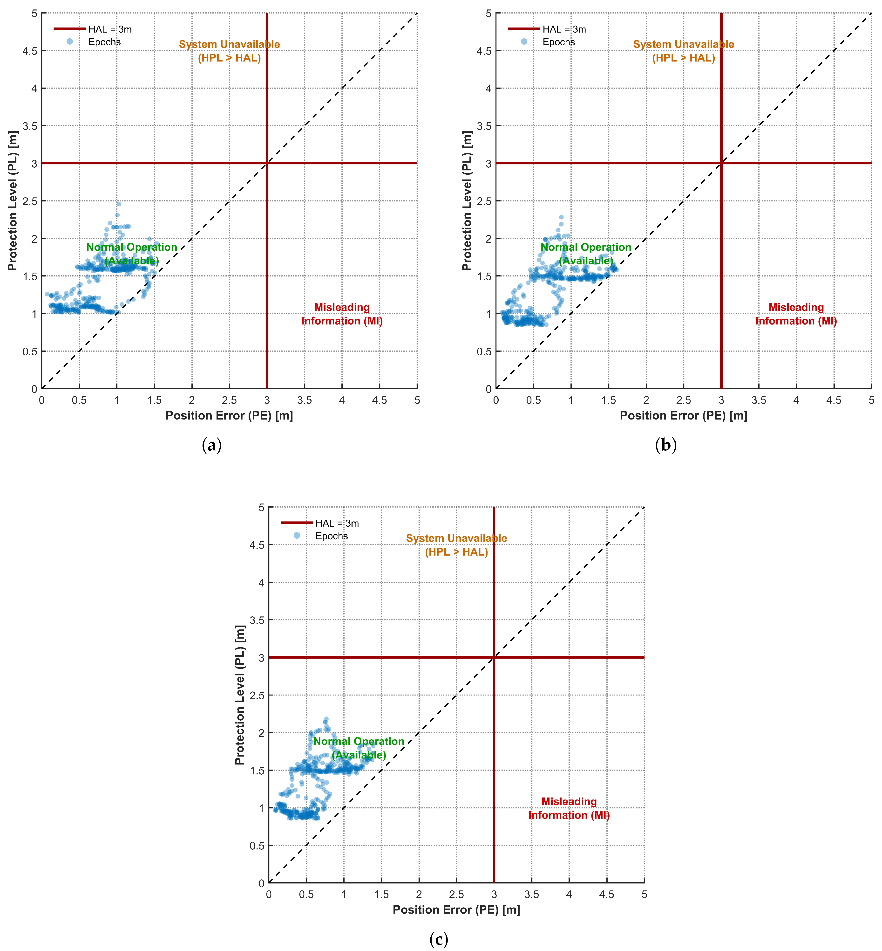
To evaluate the protection level overbounding capability and safety margin of the different filtering models, Figure 8 presents a time-series comparison of the horizontal protection level (HPL) and the true horizontal positioning error (HPE) for the three models, and Figure 9 provides the corresponding Stanford diagrams. Whether the HPL can reliably overbound the HPE is the key to evaluating positioning integrity. If the HPE exceeds the HPL, it indicates that the protection level fails to cover the true horizontal error, posing a potential risk of misleading information.

As shown in Figure 8a, the Standard KF is affected by blockage, multipath, and local NLOS propagation between 200 and 250 s. The true horizontal positioning error (HPE) increases significantly, but the corresponding HPL fails to increase synchronously, and an overbounding failure phenomenon where the HPE exceeds the HPL appears around 210 s. This occurs because the Standard KF neglects the temporal correlation of errors, causing the filter to maintain a relatively low covariance estimation in colored-noise environments. This phenomenon indicates that in obstructed degraded environments, relying solely on the conventional white noise model will lead to an underestimation of true positioning risks. Comparing Figure 8b,c, the two models introducing GMP error augmentation effectively suppress the rapid increase in HPE around 200 s, indicating that the augmented states can absorb a portion of the persistent observation biases and reduce the direct impact of anomalous observations on the position states. However, when the HPE cumulatively increases after approximately 300 s, the Typical model—due to its adoption of smaller process noise parameters—exhibits an HPL growth magnitude insufficient to keep pace with the accumulation speed of the HPE, leading to an overbounding failure around 320 s. This demonstrates that although the typical-parameter augmented model can improve estimation consistency, its safety margin remains limited when blockage and multipath are further enhanced. In contrast, the Conservative model adopts conservative parameters, enabling the filter covariance to more fully reflect the uncertainty brought by low-frequency time-correlated errors. This allows the HPL to consistently maintain a reasonable safety margin with the HPE when GNSS observation quality declines. At the same time, the HPL does not experience noticeable over-inflation, but rather maintains a relatively tight overbounding relationship with the HPE, indicating that this model can effectively balance system availability while improving integrity safety.

As can be seen from Figure 9, both the Standard KF and the Typical model experience epochs where the HPE exceeds the HPL, indicating that their protection levels fail to reliably cover the true horizontal errors in some obstructed degraded scenarios. In contrast, all data points of the Conservative model are located within the safe overbounding region, demonstrating that in this experimental data segment, the augmented model with conservative parameters can more reliably achieve the overbounding of the HPE.

Further statistics on the integrity metrics for the three models in the 200–450 s segment—which is the primary region where colored errors and overbounding failure risks occur in this study—are presented in

Table 7. Statistical integrity metrics of different models.

Metric	Standard KF	Augmented KF (Typical)	Augmented KF (Conservative)
Evaluated epochs	250	250	250
HPL/HPE bounding rate (%)	96.40	99.20	100.0
MI-like event count	9	2	0
Empirical integrity risk (%)	3.60	0.80	0.0

. Among them, the HPL/HPE bounding rate represents the proportion of epochs where the HPL successfully overbounds the true horizontal error HPE; the MI-like event count denotes the number of epochs where the HPE exceeds the HPL; and the empirical integrity risk rate represents the ratio of MI-like events to the total evaluated epochs. Considering the low-speed vehicular scenario in this study, a horizontal alert limit (HAL) of 3 m is uniformly set for the relative comparison of integrity overbounding capability and availability among the different models. It should be noted that the empirical integrity risk rate calculated based on the finite-duration vehicular experimental data in this paper is solely used for relative comparison among the different models and is not equivalent to a certification-level integrity risk. Throughout the entire segment, the availability of all three models within this statistical segment is 100%.

As can be seen from Table 7, within the 200–450 s segment, the Standard KF experiences 9 MI-like epochs where the HPE exceeds the HPL, corresponding to an HPL/HPE bounding rate of 96.40%. This indicates that under observation conditions with enhanced blockage, multipath, and NLOS propagation, the traditional white noise assumption introduces a risk that the protection level underestimates the true horizontal error. After introducing GMP error augmentation, the MI-like event count of the Typical model is reduced to 2, indicating that physical error augmentation can effectively improve the protection level overbounding capability. However, conventional empirical parameters still exhibit a slight deficiency in safety margin when low-frequency time-correlated errors are enhanced. In contrast, the Conservative model achieves a 100% empirical HPL/HPE bounding rate within this obstructed degraded segment, with both the MI-like event count and the empirical integrity risk rate being 0. This result indicates that the conservative GMP parameters, determined based on the PSD overbounding criterion, can provide a more reliable covariance baseline for protection level computation, enabling the HPL to reliably cover the HPE even in segments with enhanced colored errors. Furthermore, since the availability of all three models is 100%, it demonstrates that the integrity improvement of the Conservative model is not achieved at the expense of system availability; rather, it enhances the reliability of the protection level overbound while maintaining availability.

3.6. Controlled Fault Injection and FDE Verification

In the aforementioned real-world scenario, the MHSS fault detection mechanism remains continuously active. In the field test data without injected artificial faults, the overall number of FDE triggers is very low. The Standard KF experienced 1 trigger, while the two augmented models experienced none. Moreover, none of the three models suffered a decline in availability due to satellite exclusion. This result indicates that the aforementioned improvement in integrity overbounding does not rely on the frequent exclusion of healthy satellites. However, the types, magnitudes, and occurrence times of faults in natural scenarios are uncontrollable, making it difficult to rigorously verify the fault detection and isolation capabilities based solely on real-world natural errors. Therefore, this paper further designs a controlled pseudorange fault injection experiment to verify the detection and isolation functions of the MHSS under typical fault conditions. It should be noted that the MHSS solution separation detection logic adopted in this paper follows the standard framework. The purpose of the controlled fault injection experiment is not to re-prove the MHSS theory itself, but rather to verify whether the system can effectively respond to typical single-satellite pseudorange faults under the augmented covariance input utilized in this study.

This study sets up three types of typical pseudorange faults, all of which are injected into the pseudorange observations of a single satellite that continuously participates in the navigation solution during the injection period. The injection interval is set within the obstructed degraded segment from 300 to 360 s, and the specific fault settings are detailed in

Table 8. Controlled fault injection settings.

Fault Type	Injected Measurement	Fault Interval	Fault Model	Magnitude
Step bias	Single-satellite pseudorange	300–360 s	Constant bias	+15 m
Ramp fault	Single-satellite pseudorange	300–360 s	Linear ramp	0.5 m/s
Multipath/NLOS-like bias	Single-satellite pseudorange	300–360 s	Smooth slowly varying positive bias	9–15 m

. The first category is a step bias fault, where a fixed bias of 15 m is added to the target satellite’s pseudorange throughout the entire fault interval. This is used to simulate sudden gross errors or receiver channel anomalies. The second category is a ramp fault, where the pseudorange bias grows linearly over time at a rate of 0.5 m/s from the onset of the fault. This is used to simulate slowly developing ranging anomalies. The third category is a Multipath/NLOS-like persistent bias fault, designed to simulate the low-frequency persistent pseudorange biases caused by strong multipath or NLOS propagation in urban obstructed environments. This fault is configured as a smoothly rising positive pseudorange bias on a single satellite: it gradually reaches a stable state within 10 s after the fault initiates, and subsequently exhibits low-frequency fluctuations with a period of 80 s around a 12 m baseline bias, with a fluctuation amplitude of $\pm 3$ m. The faults injected in this section are artificially constructed anomalous single-satellite persistent biases, whose magnitudes and durations exceed the normal background error range. Therefore, such faults still need to be detected and isolated by the MHSS, rather than relying on the filter to absorb them.

To quantify the detection and isolation performance of the MHSS under controlled fault conditions, this paper calculates metrics including detection delay, isolation results, MI-like event count, and availability. Detection delay is defined as the time required for the MHSS to first detect and correctly isolate the faulty satellite after the fault injection begins; successful isolation indicates that the ultimately identified faulty satellite matches the injected one; the MI-like event count represents the number of epochs where the HPE exceeds the HPL within the fault injection interval; and availability is calculated as the proportion of epochs where HPL ≤ HAL. Successful fault isolation does not imply the absence of overbounding risks during the detection delay period; therefore, the MI-like event count can further reflect the protection level’s capability to cover true errors during the fault development and isolation process.

As shown in

Table 9. Controlled fault injection results.

Fault Type	Model	Detection Delay (s)	Isolation Success	MI-like Event Count	Availability (%)
Step bias	Standard KF	1.0	Yes	0	100.0
	Augmented KF (Typical)	1.0	Yes	0	100.0
	Augmented KF (Conservative)	1.0	Yes	0	100.0
Ramp fault	Standard KF	17.0	Yes	5	100.0
	Augmented KF (Typical)	21.0	Yes	2	100.0
	Augmented KF (Conservative)	27.0	Yes	0	100.0
Multipath/NLOS-like bias	Standard KF	9.0	Yes	3	100.0
	Augmented KF (Typical)	12.0	Yes	1	100.0
	Augmented KF (Conservative)	14.0	Yes	0	100.0

, all three models can accomplish fault detection and isolation under the three types of controlled pseudorange faults, indicating that the MHSS architecture possesses the fundamental detection capability for typical single-satellite pseudorange anomalies. For the step bias fault, because the fault introduces a distinct abrupt pseudorange change at the injection moment, all three models can complete detection and isolation within 1 s, and no MI-like events occur during the fault period. For the ramp fault, the pseudorange bias accumulates gradually over time, and its magnitude is small in the early stage of the fault; therefore, the detection delays of all three models are significantly longer than those of the step fault. Although the Standard KF can ultimately correctly isolate the faulty satellite, 5 MI-like epochs appear during its detection delay, indicating that its protection level carries an underestimation risk during the development of gradually varying faults. The augmented model adopting typical parameters reduces the MI-like event count to 2, demonstrating that the estimation consistency of the filter covariance is improved after introducing the GMP error augmented states. In contrast, although the Conservative model has a relatively longer detection delay, no instances where HPE > HPL occur during the fault injection period, indicating that its protection level can continuously cover the true horizontal errors before the fault gradually develops and is isolated. For the Multipath/NLOS-like persistent bias fault, although both the Standard KF and the Typical model can ultimately isolate the faulty satellite, they still experience 3 and 1 MI-like epochs, respectively, indicating that their protection level safety margins remain limited under persistent bias fault conditions. The Conservative model also achieves correct isolation under this type of fault, and its MI-like event count is 0, demonstrating that the conservative covariance based on the PSD overbounding criterion can provide a more reliable protection level overbound during the fault detection process.

Overall, compared with the Standard KF, the Typical model significantly reduces MI-like events under fault conditions, indicating that explicitly modeling time-correlated pseudorange errors as GMP augmented states can improve filter covariance consistency and enhance the protection level overbounding capability during faults. Building on this, the Conservative model further conducts conservative parameter tuning for key colored error parameters via the PSD overbounding criterion. Although its detection delay is slightly longer, it achieves zero MI-like events under all three types of controlled faults and maintains system availability.

It is worth further discussing the reliability and advancement of the proposed method in the context of the experimental validation. The reliability of the proposed integrity monitoring method does not solely rely on empirical fitting to the tested trajectory, but is supported by its physically interpretable and frequency-domain constrained modeling framework. Specifically, the proposed method explicitly models the temporal evolution of colored GNSS errors through Gauss-Markov state augmentation, rather than treating them as independent white noise. In addition, the conservative GMP parameters are determined under the PSD overbounding criterion, so that the augmented covariance can better reflect the low-frequency energy of persistent measurement errors. This provides a more robust covariance baseline for MHSS protection level computation and reduces the risk of HPL underestimation under time-correlated error conditions.

Despite this modeling advantage, the current field experiment is still based on a single representative vehicular trajectory. Therefore, the empirical results presented in this paper should be viewed as a case study validating the effectiveness of the proposed method in a typical transition scenario from an open-sky area to a tree-lined/building-obstructed environment. To comprehensively evaluate the generalization capability and long-term stability of the proposed architecture, future work will involve extensive testing over multiple routes, different urban geometries, longer data durations, and varying satellite visibility conditions.

4. Conclusions

Targeting the problems that GNSS observation errors exhibit temporal correlation in urban obstructed environments and that the conventional white noise model easily leads to integrity overbounding failures, this paper proposes a tightly coupled GNSS/INS integrity monitoring method based on state augmentation and frequency-domain constrained parameter tuning. This method models residual ephemeris and clock errors, tropospheric delay, and code multipath errors by introducing a first-order GMP, and sets key parameters based on the PSD overbounding criterion, thereby constructing a covariance estimation capable of reflecting the characteristics of colored errors.

Analytical results from the vehicular field test data show that, under this scenario, the proposed augmented model can improve the filter’s estimation consistency under complex observation conditions and alleviate the covariance underestimation problem present in conventional methods. Based on this, after incorporating the covariance output from the augmented filter into the MHSS framework, the protection level computation can better reflect the actual error levels, effectively reducing the risk of HPL underestimation in the obstructed degraded segment. Meanwhile, experimental results demonstrate that when conservative parameters are adopted, the system’s positioning accuracy does not exhibit noticeable degradation, and it possesses a more robust capability to suppress low-frequency persistent errors in environments with enhanced multipath and blockage. Furthermore, controlled fault injection experiments indicate that under typical pseudorange fault conditions, the proposed method can support the MHSS in achieving effective fault detection and isolation, mitigating the risk of misleading information caused by time-correlated errors.

Overall, by constructing a covariance input consistent with the error statistical characteristics at the filtering level, the method proposed in this paper enhances the reliability of the integrity overbound while ensuring system availability. It should be pointed out that the results of this paper are obtained based on a single segment of vehicular field test data and are primarily used to verify the effectiveness of the method in a typical scenario transitioning between open-sky and obstructed environments. It should be noted that the current experimental validation is based on a representative vehicular trajectory. Future work will further evaluate the proposed framework using longer-duration datasets collected from multiple routes, different urban geometries, and varying satellite visibility conditions, so as to assess its generalization capability and long-term stability.

References

1. Huang, Z.; Mou, W.; Wang, R.; Li, P.; Lyu, Z.; Ou, G. A survey of GNSS receiver autonomous integrity monitoring: Research status and opportunities. Front. Phys. 2025, 13, 1567301. [Google Scholar] [CrossRef]
2. Sun, R.; Qiu, M.; Liu, F.; Wang, Z.; Ochieng, W.Y. A Dual w-Test Based Quality Control Algorithm for Integrated IMU/GNSS Navigation in Urban Areas. Remote Sens. 2022, 14, 2132. [Google Scholar] [CrossRef]
3. Sun, R.; Zhang, W.; Zheng, J.; Ochieng, W.Y. GNSS/INS Integration with Integrity Monitoring for UAV No-fly Zone Management. Remote Sens. 2020, 12, 524. [Google Scholar] [CrossRef]
4. Reid, T.G.R.; Houts, S.E.; Cammarata, R.; Mills, G.; Agarwal, S.; Vora, A.; Pandey, G. Localization requirements for autonomous vehicles. SAE Int. J. Connect. Autom. Veh. 2019, 2, 173–190. [Google Scholar] [CrossRef]
5. Yang, L.; Sun, N.; Rizos, C.; Jiang, Y. ARAIM Stochastic Model Refinements for GNSS Positioning Applications in Support of Critical Vehicle Applications. Sensors 2022, 22, 9797. [Google Scholar] [CrossRef] [PubMed]
6. Sun, R.; Fu, L.; Cheng, Q.; Chiang, K.W.; Chen, W. Resilient pseudorange error prediction and correction for GNSS positioning in urban areas. IEEE Internet Things J. 2023, 10, 9979–9988. [Google Scholar] [CrossRef]
7. Wang, H.; Leng, J. A brief review on the development of Kalman filter. In Proceedings of the 2018 Chinese Control and Decision Conference (CCDC), Shenyang, China, 9–11 June 2018; pp. 1–6. [Google Scholar]
8. Zhou, Z.; Wu, J.; Li, Y.; Fu, C.; Fourati, H. Critical issues on Kalman filter with colored and correlated system noises. Asian J. Control 2018, 20, 2421–2432. [Google Scholar] [CrossRef]
9. Jiang, Y. RAIM Fault Detection and Exclusion with Spatial Correlation for Integrity Monitoring. Remote Sens. 2023, 15, 176. [Google Scholar] [CrossRef]
10. Miller, C.; O’Keefe, K.; Gao, Y. Time correlation in GNSS positioning over short baselines. J. Surv. Eng. 2012, 138, 10–17. [Google Scholar] [CrossRef]
11. Zhu, Z.; Taylor, C.J. Conservative uncertainty estimation in map-based vision-aided navigation. IEEE Trans. Aerosp. Electron. Syst. 2017, 53, 941–949. [Google Scholar] [CrossRef]
12. Shao, J.; Yu, F.; Zhang, Y.; Sun, Q.; Wang, Y.; Chen, W. Robust Sequential Integrity Monitoring for Positioning Safety in GNSS/INS Integration. IEEE Sens. J. 2024, 24, 15145–15155. [Google Scholar] [CrossRef]
13. Kermarrec, G.; Jain, A.; Schön, S. Kalman filter and correlated measurement noise: The variance inflation factor. IEEE Trans. Aerosp. Electron. Syst. 2021, 58, 766–780. [Google Scholar] [CrossRef]
14. Rife, J.; Misra, P. Impact of time-correlation of monitor statistic on continuity of safety-critical operations. Navigation 2012, 59, 303–315. [Google Scholar] [CrossRef]
15. Hajiyev, C. INS’s error compensation via measurement differencing Kalman filter. IEEE Trans. Instrum. Meas. 2022, 71, 8503408. [Google Scholar] [CrossRef]
16. Petovello, M.G.; O’Keefe, K.; Lachapelle, G.; Cannon, M.E. Consideration of time-correlated errors in a Kalman filter applicable to GNSS. J. Geod. 2009, 83, 51–56. [Google Scholar] [CrossRef]
17. Wang, X.; Pan, Q. Nonlinear Gaussian filter with the colored measurement noise. In Proceedings of the 17th International Conference on Information Fusion (FUSION), Salamanca, Spain, 7–10 July 2014; pp. 1–7. [Google Scholar]
18. Garcia Crespillo, O.; Joerger, M.; Langel, S. Overbounding GNSS/INS integration with uncertain GNSS Gauss-Markov error parameters. In Proceedings of the 2020 IEEE/ION Position, Location and Navigation Symposium (PLANS), Portland, OR, USA, 20–23 April 2020; pp. 481–489. [Google Scholar]
19. Gallon, E.; Khanafseh, S.; Pervan, B.; Joerger, M. Performance assessment of fault free recursive ARAIM with high-integrity time-correlated measurement error models. In Proceedings of the 35th International Technical Meeting of the Satellite Division of The Institute of Navigation (ION GNSS+ 2022), Denver, CO, USA, 19–23 September 2022; pp. 1455–1466. [Google Scholar]
20. Uwineza, J.-B.; Farrell, J.A. RAIM and Failure Mode Slope: Effects of Increased Number of Measurements and Number of Faults. Sensors 2023, 23, 4947. [Google Scholar] [CrossRef] [PubMed]
21. Wang, H.; Cheng, Y.; Cheng, C.; Li, S.; Li, Z. Research on Satellite Selection Strategy for Receiver Autonomous Integrity Monitoring Applications. Remote Sens. 2021, 13, 1725. [Google Scholar] [CrossRef]
22. Vanderwerf, K. FDE using multiple integrated GPS/inertial Kalman filters in the presence of temporally and spatially correlated ionospheric errors. In Proceedings of the 14th International Technical Meeting of the Satellite Division of The Institute of Navigation (ION GPS 2001), Salt Lake City, UT, USA, 11–14 September 2001; pp. 2676–2685. [Google Scholar]
23. Blanch, J.; Walter, T.; Enge, P.; Lee, Y.; Pervan, B.; Rippl, M. Baseline Advanced RAIM User Algorithm and Possible Improvements. IEEE Trans. Aerosp. Electron. Syst. 2015, 51, 713–732. [Google Scholar] [CrossRef]
24. Groves, P.D. Principles of GNSS, Inertial, and Multisensor Integrated Navigation Systems, 2nd ed.; Artech House: Norwood, MA, USA, 2013. [Google Scholar]
25. U.S. Department of Defense. Global Positioning System Standard Positioning Service (SPS) Performance Standard, 5th ed.; U.S. Department of Defense: Washington, DC, USA, 2020.
Figure 1. Overall flowchart of the physical-error-augmented GNSS/INS tightly coupled integrity monitoring system.
Remotesensing 18 01564 g001
Figure 2. Schematic diagram of the MHSS filter structure.
Remotesensing 18 01564 g002
Figure 3. Schematic diagram of the MHSS fault exclusion principle.
Remotesensing 18 01564 g003
Figure 4. Schematic diagram of the experimental vehicle trajectory.
Remotesensing 18 01564 g004
Figure 5. PSD comparison of empirical multipath residuals and GMP models.
Remotesensing 18 01564 g005
Figure 6. Time series of positioning errors for three different models: (a) Standard KF; (b) Typical Model; (c) Conservative Model.
Remotesensing 18 01564 g006
Figure 7. Time series of position NEES for three different models: (a) Standard KF; (b) Typical Model; (c) Conservative Model.
Remotesensing 18 01564 g007
Figure 8. Time-series comparison of HPL and HPE for three different models: (a) Standard KF; (b) Typical Model; (c) Conservative Model.
Remotesensing 18 01564 g008
Figure 9. Stanford diagram for three different models: (a) Standard KF; (b) Typical Model; (c) Conservative Model.
Remotesensing 18 01564 g009