Article

Linking Plant Traits to Fire Potential Mapping: A Feasibility Study in Australian Ecosystems

1
Quasar Science Resources S.L., Calle Chile 8, Las Rozas de Madrid, 28290 Madrid, Spain
2
Institute of Forest Science (ICIFOR-INIA), CSIC, Carretera de La Coruña km 7.5, 28040 Madrid, Spain
3
ETSI Montes, Forestal y del Medio Natural, Universidad Politécnica de Madrid (UPM), Ramiro de Maeztu, 28040 Madrid, Spain
4
Fenner School of Environment and Society, College of Systems and Society, The Australian National University, Canberra, ACT 2601, Australia
5
Bushfire Research Centre of Excellence, The Australian National University, Canberra, ACT 2601, Australia
6
School of Engineering, College of Systems and Society, The Australian National University, Canberra, ACT 2601, Australia
*
Author to whom correspondence should be addressed.
Remote Sens. 2026, 18(10), 1546; https://doi.org/10.3390/rs18101546
Submission received: 16 March 2026 / Revised: 7 May 2026 / Accepted: 8 May 2026 / Published: 13 May 2026
(This article belongs to the Special Issue Hyperspectral Data Analysis of Vegetation and Soil Monitoring)

Highlights

What are the main findings?
  • Structural and biochemical plant traits (leaf mass per area, carbon, and cellulose) are effective predictors of eucalypt flammability.
  • Plant traits indices derived from hyperspectral imagery were successfully used to generate flammability maps.
What is the implication of the main finding?
  • The proposed framework represents a novel approach for mapping fuel flammability.

Abstract

Given the increasing frequency, severity, and socioecological impacts of wildfires, there is an urgent need for robust frameworks to better characterize fire behavior and flammability patterns across ecosystems to support early warning, mitigation, and management strategies. However, flammability remains difficult to quantify and scale, as it involves multiple interacting components that are typically measured at the bench scale. This study aimed to establish empirical links between spectral information, plant traits, and flammability metrics, and to scale these relationships to satellite imagery to translate these metrics into a spatial context. We combined laboratory spectroscopy, plant trait measurements including leaf mass per area, carbon, and cellulose, and combustion experiments using a simple and reproducible burning device. In total, 84 samples were collected and analysed, allowing us to characterise how spectral signatures relate to vegetation traits and fire behaviour. Spectral indices were developed to estimate plant traits, which were subsequently used as predictors in flammability models. These models were then transferred to Environmental Mapping and Analysis Program (EnMAP) hyperspectral imagery to derive spatial estimates across eucalypt forests and grasslands of the Australian Capital Territory (ACT). Spectral information distinguished fuel types and captured variability of the plant traits, while these traits showed associations with combustion behaviour. Based on these links, the best-performing model predicted the rate of temperature increase, a combustibility metric, in eucalypt forests (R2 = 0.70; Root Mean Square Error = 32.48 °C/s). In contrast, grassland models showed limited predictive performance, likely due to weaker relationships between plant traits and flammability metrics. Overall, this study demonstrates a practical and scalable approach for deriving flammability maps from hyperspectral and in situ data, highlighting the potential of plant-trait-based remote sensing. The resulting maps should not be interpreted as standalone fire risk products, but rather as a characterization of the structural and biochemical drivers of flammability. The main constraint of this work is the limited sample size. Future research should expand spatial and temporal coverage to better capture vegetation variability and enable the inclusion of independent validation datasets. Exploring alternative combustion protocols and testing more advanced spectral modelling approaches for trait estimation would provide additional insights.

1. Introduction

Wildfires have been a part of Earth’s environment since the evolution of terrestrial plants, shaping the composition and structure of many ecosystems [1,2,3]. Traditional Indigenous fire practices, which often involved regular, low-intensity burns, provide the foundation for many modern prescribed-burning strategies, restoring ecological balance, reducing fuel loads, and supporting biodiversity [4,5].
Nevertheless, recent decades have witnessed a marked increase in the frequency and intensity of extreme wildfires worldwide, even in ecosystems historically considered less fire-prone, such as rainforests, wetlands, and boreal forests, where vegetation structure and moisture regimes had previously limited fire occurrence [6]. This shift has led to multiple consequences, including the rise in fire-related carbon emissions [6], alterations in land surface temperature [7], and an accelerated loss of forest cover and ecological value, particularly in vulnerable biomes [8,9]. Wildfires also lead to injuries, fatalities, long-term respiratory illnesses, and smoke-related mortality [10,11,12]. As a whole, economic losses from wildfire disasters continue to rise globally [13].
Given the escalating frequency, severity, and socioecological impacts of wildfires, there is an urgent need for predictive tools capable of anticipating fire behavior and flammability patterns across diverse ecosystems to support early warning, mitigation, and management strategies such as prescribed burning plans.
Forest fuel flammability, defined as the inherent capacity of plant biomass to ignite and sustain combustion [14], is a key determinant of wildfire risk and fire behavior [15,16]. Importantly, flammability cannot be captured by a single variable, as it encompasses multiple, interrelated components. Plant flammability comprises four components: ignitability (the ease with which material ignites), combustibility (the rate of energy release during combustion), sustainability (the duration and intensity with which combustion is maintained), and consumability (the proportion of biomass consumed during combustion) [14,17]. Each component can be quantified using distinct experimental metrics and units, which vary widely across studies. Some laboratory approaches include the use of mass loss calorimeters [18] or epiradiators [19] for assessing leaf flammability. These devices expose samples to high temperatures under controlled conditions. Other methods, such as the ‘grid’ method, quantify shoot-level flammability but rely on drying samples prior to the experiment to ensure ignition and sustained combustion [20,21,22]. Such approaches, based on pre-drying, exclude moisture-driven effects and primarily quantify structural and chemical characteristics.
Importantly, flammability traits differ among species, reflecting variations in plant structure, water content, and biochemical composition [23,24]. Most flammability studies are conducted at the bench scale, focusing on leaves, shoots, or small fuel beds. While such experiments represent an essential step toward understanding fire behavior, scaling up leaf- or shoot-level measurements to landscape-scales remains a major challenge [15,25,26,27]. Burning entire plants provides a more integrative assessment of flammability but is often logistically complex and costly, particularly for trees and large shrubs [16].
Physiological, morphological, and chemical plant characteristics, collectively referred to as plant traits, can be used as predictors of fuel flammability [23,24,28,29]. Among these traits, fuel moisture content (FMC) remains the most widely used due to its strong influence on ignition and combustion dynamics [16,24]. Additionally, the field of Pyro-Ecophysiology has emerged to provide a mechanistic framework for understanding how plant water and carbon cycles mediate flammability [30,31,32]. From a remote sensing perspective, mapping plant traits that influence flammability, such as plant water and carbon content, offers a promising pathway for integrating physiological information into fire behavior and effects models [32]. Although such integration has been conceptually proposed, it has rarely been implemented in practice. Spectroscopy provides a powerful means to estimate these traits from spectral information, with techniques such as Partial Least Squares Regression (PLSR) widely applied at the leaf and canopy levels [33,34], and more recent machine learning approaches enhancing predictive accuracy and transferability across vegetation types [35,36,37].
In this feasibility study, we combined spectroscopy-based trait estimation with laboratory-based traits to predict vegetation flammability. We focused on two characteristic Australian ecosystems, eucalypt forests and grasslands, and generated flammability maps using imagery from the Environmental Mapping and Analysis Program (EnMAP) satellite. Our overarching hypothesis is that spectral information can ultimately be used to produce flammability maps, linking plant functional traits to fire potential.

2. Materials and Methods

2.1. Study Area and Sampling Design

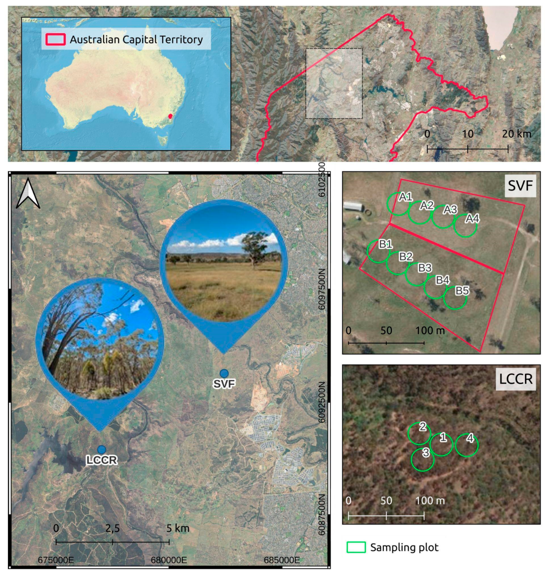
Two accessible study sites near Canberra (Australian Capital Territory (ACT)), a rewilded eucalypt forest and a grassland, were selected to develop the flammability maps. The eucalypt forest was located in the Lower Cotter Catchment Reserve (LCCR, Figure 1), a former plantation regenerated after a wildfire that affected the region in 2003 [38]. The grassland is located in Spring Valley Farm (SVF, Figure 1), a farm southwest of Canberra leased by the Australian National University for research activities. At the time of sampling, the site featured a homogeneous mix of native and introduced grass and weed species.
Sampling plots were established in homogeneous vegetation areas within each site. Each plot had a radius of 15 m, consistent with the EnMAP) satellite spatial resolution (30 m, see Section 2.5). Given the geometric accuracy of the sensor (12.5 m or better) and the homogeneity of the sites, this plot size was sufficient to minimize edge effects and ensure site representativeness.
In the LCCR, we selected a homogeneous area oriented towards the north, minimising topography shading during satellite overpasses. Leaf samples from the two main species of eucalypts (Eucalyptus mannifera and Eucalyptus melliodora) were collected, except in Plot 3, where only E. melliodora was present. Litter samples were also collected in each plot, consisting of dead eucalypt leaves found on the ground. The total fractional cover of each species and litter was recorded separately per vertical stratum.
Two paddocks (A and B, Figure 1) were selected at SVF. Four sampling plots were placed in paddock A and five in paddock B; in paddock A, a fifth plot was not established because standing water was present in the intended location during the first visit. In plot B3, only the dominant species was sampled, as the second-most abundant species was too scarce to be meaningfully sampled. Species identification is provided in the Supplementary Materials.
The samples were collected randomly inside the plot from the two most abundant species, from at least five different individuals per species. The species cover (%) within each plot was visually estimated and recorded. This enables analyses at the species (sample) level while supporting plot-level aggregation, which is more appropriate for satellite-based modelling. Each sample consisted of 5 to 20 g of plant material. In the case of trees, leaves from the canopy were collected and, for grasses, the entire individual was collected. All samples were labelled, sealed in plastic bags, and transported in coolers to the laboratory on the same day.
Three field campaigns were conducted on the 4th and 19th of March, and on the 3rd of April in 2025, scheduled to coincide as closely as possible with EnMAP overpasses under cloud-free conditions.

2.2. Laboratory Experiments

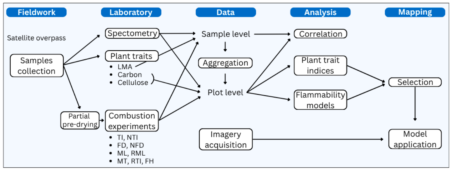
Three data types were collected for this study: spectral reflectance, biophysical plant traits, and flammability metrics (Figure 2). The spectral information was measured for each sample using a spectroradiometer (HR-1024i from Spectra Vista Corporation, (SVC), New York, NY, USA) with a leaf clip attachment. This instrument covers a range between 400 and 2500 nm. Three replicate scans per sample were taken to avoid irregular features [24,34].
The leaf mass per area (LMA) was determined as a structural trait, and carbon and cellulose as chemical traits. This selection was based on their relationship with flammability [23,24]. FMC was also measured as a control variable but was not analysed in terms of its variability or included as a predictor in the models. Samples were fresh-weighted, dried at 105 °C for 24 h in an oven, and weighed again to determine FMC [39]. For the LMA, the Leaf Area (LA), defined as the projected surface area of the leaf, was measured first with a Logitech USB HD Webcam (Logitech, Lausanne, Switzerland) controlled by custom LabVIEW NXG 5.0 Community Edition software (National Instruments Corporation, Austin, TX, USA). For grasses, LA of the whole plant was measured to account for the difficulty in separating leaf blades from stems and to better represent the functional fuel unit.
F i e l d F M C ( % ) = F r e s h w e i g h t D r y w e i g h t D r y w e i g h t × 100
L M A ( g c m 2 ) = D r y w e i g h t L e a f a r e a
Carbon and cellulose were calculated at a plot level by mixing each species in proportion to its relative coverage within each plot. For grass plots, this was done by summing the absolute cover of all sampled species and expressing each species’ cover as a proportion of that total, so that relative coverage values sum to 100%. In forest plots, the contribution of litter was first calculated as a proportion of the area not occupied by the tree canopy, after which the same procedure was applied so that all measured components’ relative coverage summed to 100%. This approach ensured that the contributions of all strata reflected both plot structure and the effective visibility of each layer to satellite sensors.
Afterwards, the compound samples were ground to a fine, homogeneous powder using a cryogenic bead grinder. Cellulose content was extracted and quantified using the method described by [40], which involves sequential extraction to remove soluble compounds using a nitric acid digestion and centrifugation, followed by acid hydrolysis and quantification using spectrophotometry. Total carbon content was determined following [41], using a pyrolysis analysis. The process consists of weighing ground samples into crucibles appropriate for the analyser and then pyrolysing them at high 900 °C. The instrument measures released carbon during the oxidation process as a percentage of dry mass.

2.3. Combustion Experiments

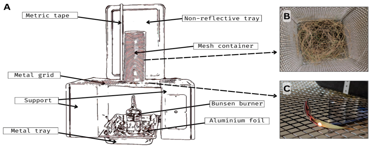
Two experimental setups were used, depending on vegetation type. For eucalypt leaves (both live and dead, i.e., litter), individual samples were placed on a metal grid positioned above a Bunsen burner (Figure A1). For grasses, samples were aggregated at the plot level and placed inside a mesh container, resting against the grid, following [42] (Figure A1B). In both setups, the leaf sample or the mesh container holding the grass sample was exposed to the flame until ignition occurred, at which point the burner was turned off.
Five replicates were conducted for each sample, thus ensuring enough variability to represent field data. Vegetation samples were previously oven-dried at 40 °C for four days before the flammability experiments, to ensure ignition and sustained combustion. As a result, the experiments quantify intrinsic flammability driven by structural and chemical properties, rather than moisture effects. A subsample of the material was used to determine the fuel moisture content at the time of the experiment; this value is hereafter referred to as residual FMC, in contrast to the field FMC measured on fresh samples. Nine flammability metrics were measured in these experiments (see Table 1). More information regarding the combustion experiments is provided in Appendix A.

2.4. Dataset Compilation

The dataset was constructed by integrating spectral data, biophysical information, and flammability metrics (Table 2). Each sample was assigned a standardised filename encoding key metadata including field collection date, sample type, and plot identifiers, ensuring traceability throughout the analysis.
The relative coverage values (see Section 2.2) were used as weights to compute plot-level averages for all measured parameters. Because the method is intended for optical remote sensing, the reflectance contribution of each stratum was weighted according to its actual visibility to the satellite: upper layers were averaged first, and lower strata were weighted based on the gap fraction left by the canopy and their relative coverage within those gaps.
Spectral data (see Section 2.2) were pre-processed by applying a Savitzky–Golay filter to correct artifacts in the sensor-overlap regions (~1000 and ~1900 nm). The three spectral scans per sample were then averaged to obtain a single reflectance signature, which was incorporated at the sample level.
LMA was measured at the sample level, whereas biochemical traits (cellulose and carbon) were analysed only at the plot level after compositing species according to their relative coverage (see Section 2.2).
Flammability metrics were obtained from five experimental replicates per sample (see Section 2.3), with the replicate mean retained as the final measurement. For grasses, combustion experiments were conducted on species mixtures at the plot level; consequently, grass flammability metrics were included only in the plot-level dataset.
To generate plot-level values for LMA, sample-level observations were aggregated using their relative coverage within each plot, as described previously. This weighting procedure ensured that the final plot-level dataset reflected the effective contribution of each species to the optical signal expected at the satellite scale.

2.5. Mapping Plant Trait Indices

Flammability map generation involved three main steps. First, spectral indices representative of the biophysical plant traits (plant trait indices) were derived. Second, statistical models relating plant traits to flammability metrics were developed (see Section 2.6). Finally, the selected plant trait indices were computed using EnMAP imagery and used as predictors in the flammability models to produce flammability maps (Section 2.7). All analyses were performed separately for grasses and eucalypts at the plot level.
EnMAP satellite [43] is an imaging spectrometer that records reflectance values across 224 bands in the 420–2450 nm range. It uses two overlapping spectrometers, one for the Visible and Near-Infrared (VNIR) and one for the Short-wave infrared (SWIR), providing a spectral resolution of 6.5 nm (VNIR) and 10 nm (SWIR), and a spatial resolution of 30 × 30 m.
The following level 2A products (orthorectified and atmospherically corrected for land) were downloaded through the D-SDA Access Services/EOWEB Geoportal:
  • ENMAP01-____L2A-DT0000118805_20250313T005021Z_003_V010502_20250321T025109Z;
  • ENMAP01-____L2A-DT0000122260_20250401T004343Z_003_V010502_20250403T234200Z;
  • ENMAP01-____L2A-DT0000123007_20250405T004720Z_003_V010502_20250409T025658Z.
A water and cloud mask was applied to all scenes prior to analysis.
To ensure compatibility, the EnMAP spectral response function was used to convolve SVC reflectance measurements to EnMAP-equivalent bands spectrally. This convolution was performed in Python 3.10.12 using a custom function that applied Gaussian weighting to each SVC wavelength according to the EnMAP band’s central wavelength and full width at half maximum (FWHM), effectively reproducing the sensor’s spectral response.
The approach for calculating plant trait indices consisted of computing all possible two-band combinations to derive the difference (B1−B2), the simple ratio (B1/B2), and the normalised difference index (NDI, (B1 − B2)/(B1 + B2)). For each trait and index combination, linear regressions were performed to obtain the coefficient of determination (R2) and root mean square error (RMSE), quantifying the explanatory power of each index. Bands affected by strong atmospheric absorption (760 nm, 930–950 nm, 1117–1154 nm, 1346–1490 nm, and 1800–1950 nm) were excluded to ensure reliable spectral relationships. Indices were selected not only based on statistical performance but also on the visual quality of the resulting EnMAP images, favouring indices that produced spatially coherent, low-noise patterns and avoided artifacts, thereby ensuring meaningful spatial interpretation.
Selected trait indices were then computed from EnMAP imagery.

2.6. Flammability Models

Models of flammability were developed for each of the flammability metrics (Table 1) by testing all possible combinations of plant traits as predictors in single and multiple linear regressions. Model selection was based on predictive performance (R2, RMSE and Akaike Information Criterion (AIC)) as well as the individual performance of each plant trait index used as a predictor.

2.7. Flammability Maps

The ACTGOV Vegetation Map 2023 from the ACT Government Geospatial Data Catalogue (https://actmapi-actgov.opendata.arcgis.com/datasets/ACTGOV::actgov-vegetation-map-2023/about accessed on 15 May 2025) was used to mask the areas where eucalypt forests and grasslands are present (Figure S1, Supplementary Materials).
Flammability models developed for each vegetation type were then applied using the corresponding plant trait indices. Because the flammability models were fitted using plant traits expressed in real units, whereas spectral indices are unitless, each index was converted back to real trait units via the model intercept prior to prediction.
Finally, due to the feasibility nature of the study and the limited dataset, independent validation of the models was not possible. Instead, the resulting maps were evaluated using descriptive statistics (range, mean and standard deviation).

3. Results

A total of 84 vegetation samples and 252 spectral samples were collected during the field campaign, and 300 combustion experiments were performed.

3.1. Reflectance Spectra

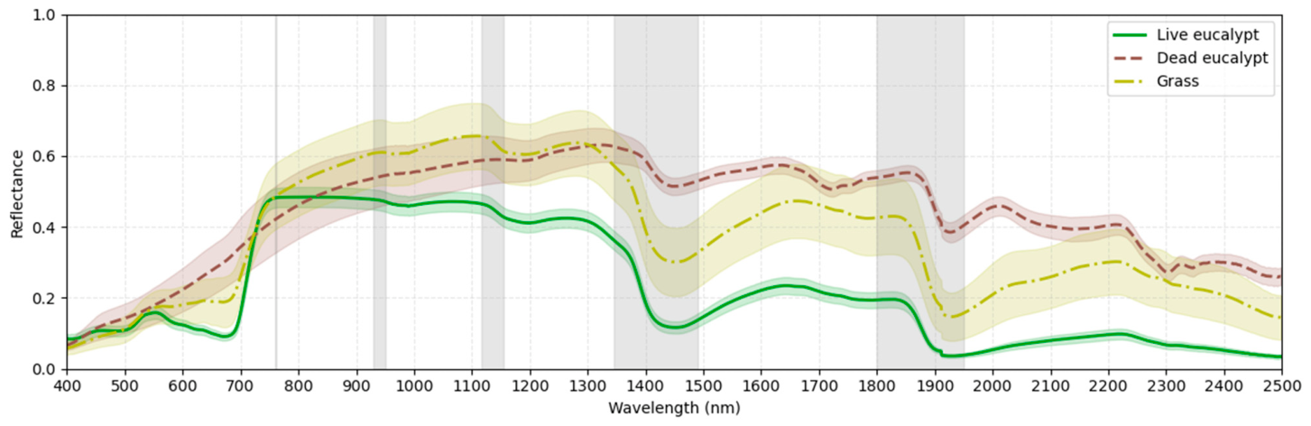
The Savitzky–Golay smoothing parameters that produced the best results were a window length of 21 and a polynomial order of 2. The averaged smoothed spectra for each fuel type (Figure 3) displays higher reflectance values in grasses and dead eucalypt compared to live eucalypt, particularly in the near-infrared (NIR, ~750–1400 nm) and shortwave infrared (SWIR, ~1450–2400 nm) regions. Grasses also exhibited greater spectral variability than eucalypts. These spectral differences are consistent with known variations in moisture content and structure across fuel types, providing a basis for examining their relationship with vegetation traits in the next section.

3.2. Plant Traits

LMA, which represents how much mass is packed into a given leaf area, was very similar between live and dead eucalypt (Table 3), as expected given that both are eucalypt leaves, while grasses exhibited lower LMA values.
Regarding biochemical traits, carbon content showed higher average values in eucalypts than in grasses. In contrast, cellulose content was higher on average in grasses, although the maximum values and overall variability were greater in eucalypts.

3.3. Combustion Experiments

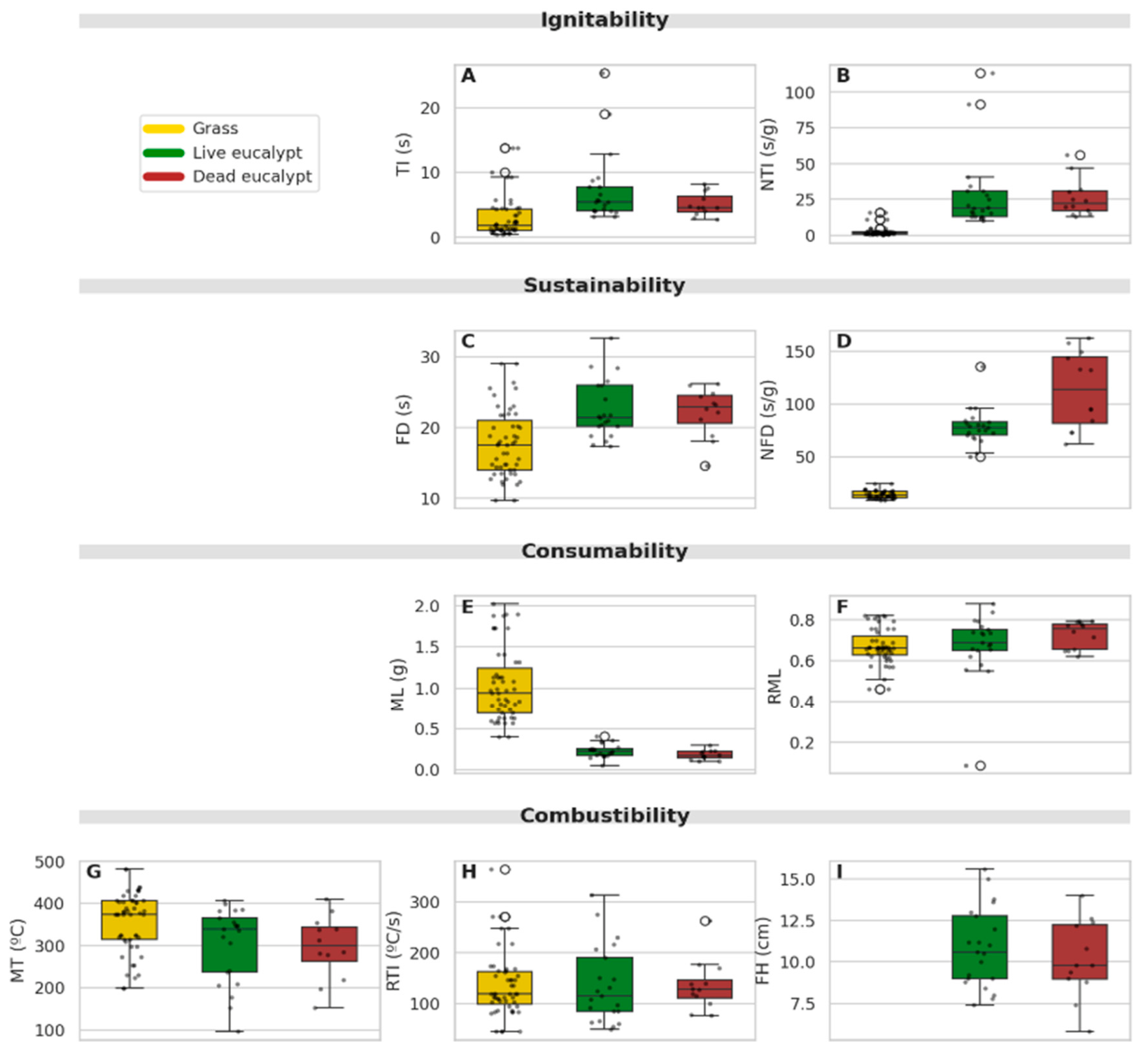
Overall, eucalypt samples behaved differently from grasses in the combustion experiments. Live and dead eucalypt leaves showed relatively similar flammability, likely influenced by the partial drying during sample preparation (see Section 2.3). Grasses exhibited much faster ignition, with dead eucalypt leaves taking roughly one and a half times longer to ignite than grasses, and live eucalypt leaves taking about twice as long (Figure 4A). After normalisation (normalised time to ignition), this contrast became even more pronounced, with eucalypts reaching values up to ten times higher than grasses (Figure 4B), and variability in grasses markedly reduced. Sustainability was greater in eucalypts (Figure 4C,D), especially after normalisation, where flaming duration increased between five and eight times relative to grasses, again with lower variability in the grass samples. In other words, the grass ignited and burned rapidly, as expected. For consumability, grasses lost approximately five times more mass than eucalypt samples (Figure 4E), although relative mass loss was comparable among fuel types (Figure 4F). Combustibility was slightly higher in grasses in terms of maximum temperature (Figure 4G), while the rate of temperature increase was relatively similar across all fuel types (Figure 4H). Flame height, measured only for eucalypt leaves, showed little difference between live and dead fuels (Figure 4I).
To assess whether the observed differences in flammability among vegetation types were statistically significant, Analysis of Variance (ANOVA) or Kruskal–Wallis tests were applied depending on data normality (Table S3 Supplementary Materials). Most flammability metrics showed significant differences among vegetation types, whereas relative mass loss, rate of temperature increase, and flame height did not (Table 4). Post hoc comparisons revealed that grass fuels differed from both live and dead eucalypt fuels for most metrics, while live and dead eucalypt fuels generally did not differ from each other. Exceptions included relative mass loss and rate of temperature increase, for which no differences were detected among any vegetation types, and maximum temperature, which showed no differences except for a weak contrast between dead eucalypt and grass fuels.

3.4. Relationships Among Spectral Information, Plant Traits, and Flammability

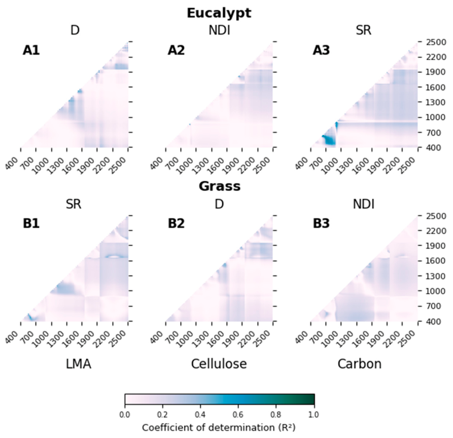
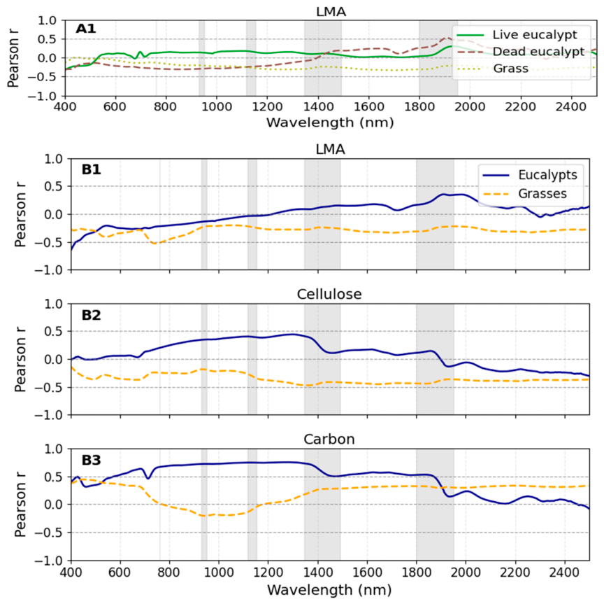
Correlation between plant traits and spectral information was assessed at both the sample and plot levels and plotted as a correlogram (Figure 5). Plant traits showed distinct behaviours between vegetation types. In eucalypts, carbon content was strongly and positively correlated with reflectance from 600 to 1900 nm (Figure 5, B3; r ≈ 0.6), and cellulose displayed the same pattern but more weakly (Figure 5, B2; r ≈ 0.2). In contrast, grasses exhibited broadly negative correlations with cellulose across the spectrum (Figure 5, B2; r ≈ −0.4) and weaker negative correlations with LMA (Figure 5, A1 and B1; r ≈ −0.3). Interestingly, carbon in grasses showed positive correlations in two spectral regions—400–730 nm and 1200–2400 nm—despite the negative pattern observed for the other traits (Figure 5, B; r ≈ 0.3).
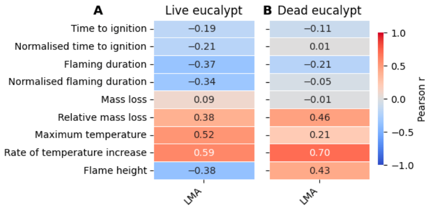
The relationship between plant traits and flammability metrics was assessed using correlation analysis. Overall, correlations between LMA and flammability in eucalypts at the sample level were weak, particularly for ignitability, sustainability, and consumability (Figure 6). Nevertheless, live and dead eucalypt leaves showed broadly similar trends in how their traits related to flammability, consistent with their comparable behavior in the combustion experiments (see Section 3.3). LMA displayed a strong positive correlation with the rate of temperature increase in both live and dead eucalypt, suggesting that denser leaves heat up more rapidly during combustion. Flame height was also positively correlated with LMA in dead leaves but showed a negative correlation in live leaves.
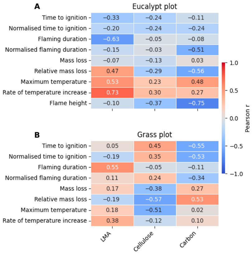
The correlation was determined at the plot level, including the biochemical traits and the grasses that performed the burning experiments, directly aggregated (Figure 7). In general terms for the eucalypts, ignitability and sustainability showed weak negative correlations with LMA, cellulose, and carbon, indicating that denser and more carbon- and cellulose-rich leaves tend to ignite faster and sustain combustion for shorter periods. In addition, maximum temperature and rate of temperature increase were positively correlated with these traits, suggesting hotter and more rapidly developing flames (Figure 7A). In contrast, flame height followed an inverse trend, with higher trait values associated with shorter flames, particularly for carbon (r = −0.75).
Correlations were generally stronger for eucalypts at the plot level than at the separated (live and dead) level, suggesting that aggregation enhances overall relationships. For example, the correlation between the rate of temperature increase and LMA increased from 0.59 (live) and 0.70 (dead) to 0.73 when aggregated, while the relationship between flaming duration and LMA strengthened from −0.37 (live) and −0.21 (dead) to −0.63.
In grasses, the correlations had different patterns compared to eucalypt (Figure 7B). LMA was generally positively correlated with the flammability metrics, and cellulose and carbon displayed opposed patterns (Figure 7B). For example, ignitability was negatively correlated with cellulose and positively correlated with carbon, and relative mass loss showed the same pattern. LMA was positively correlated with flaming duration, indicating that higher dry matter content was associated with longer combustion, in contrast to the pattern observed in eucalypts.

3.5. Mapping Plant Trait Indices

Three operations (difference, simple ratio, and normalised difference) were used to compute spectral indices and relate them to plant traits. From this point onward, all analyses were performed at the plot level. For eucalypts, LMA was best predicted using bands near 1760 nm (B1) and 1780 nm (B2) (R2 = 0.55), with weaker relationships also found around 2340–2430 nm (Figure 8, C1). The cellulose index performed best with bands at 680 nm (B1) and 690 nm (B2) (R2 = 0.57), with additional combinations around 1620–1660 nm showing moderate performance (Figure 8, D1). Carbon indices achieved R2 values near 0.70, especially with band pairs around 520–570 nm and 730–740 nm (Figure 8, E1). Although R2 varied across indices, the RMSE values for the highest R2 indices were very similar. The indices selected for the flammability models are listed in Table 5.
For grasses, LMA indices showed moderate predictive ability (R2 up to 0.51) and were associated exclusively with bands around 450 nm (B1) and 510 nm (B2) (Figure 8, C2). Cellulose indices were related to bands near 1210 nm (B1) and 1280 nm (B2), reaching a maximum R2 of 0.41 (Figure 8, D2). Carbon indices showed the lowest performance among the plant traits, with indices associated with bands around 1230 nm (B1) and 1270 nm (B2) (Figure 8, E2). The indices selected (Table 5) were then used as predictors in the flammability models to generate the flammability maps.

3.6. Flammability Models

For each flammability metric (Table 1), regression models were fitted using all possible combinations of plant traits measured in the laboratory. This resulted in 63 models for eucalypts (9 response variables × 7 combinations) and 56 models for grasslands (8 response variables × 7 combinations).
In the eucalypt models (n = 12), the highest coefficient of determination was obtained for the rate of temperature increase (R2 = 0.70) using LMA, cellulose, and carbon as predictors (Model A1, Table 6). A reduced model including only LMA and cellulose (Model A2) showed very similar performance (R2 = 0.68), indicating a limited contribution of carbon to this metric. This was further supported by the minimal change in the AIC (91.53 to 90.36) and RMSE (32.48 °C/s to 33.61 °C/s) despite the reduction in model complexity. Overall, LMA emerged as the most influential predictor of the rate of temperature increase, as models retaining this trait consistently outperformed those excluding it, in agreement with the correlation patterns observed previously (Figure 7A).
Flame height was the second-best-performing flammability metric, with the full model (LMA, cellulose, and carbon) reaching R2 = 0.60 (Model B1). A reduced model retaining only cellulose and carbon (Model B2) achieved a comparable performance (R2 = 0.59), while slightly increasing RMSE (from 1.26 cm to 1.28 cm) and lowering AIC (from 13.62 to 11.89), indicating a similar fit with reduced complexity. Across model combinations, carbon showed the strongest and most consistent influence on flame height, aligning with the correlation results (Figure 7A), while LMA showed the weakest influence.
Based on these results, the four models A1, A2, B1, and B2 were selected for further analysis. Relative mass loss and maximum temperature also reached moderate performance (R2 > 0.50) but were not retained to focus on the best-performing models.
Overall, the flammability models for grasses performed worse than those developed for eucalypts despite having a larger sample size (n = 26). The best performance was obtained when predicting the relative mass loss using LMA, cellulose, and carbon (R2 = 0.42). Carbon was discarded as a predictor due to its poor performance as a plant-trait index (R2 = 0.37). After its removal, the next best model predicted the maximum temperature using the remaining two traits, achieving an R2 of 0.36. Due to this limited predictive performance, grassland flammability models were not retained for spatial application.

3.7. Flammability Maps

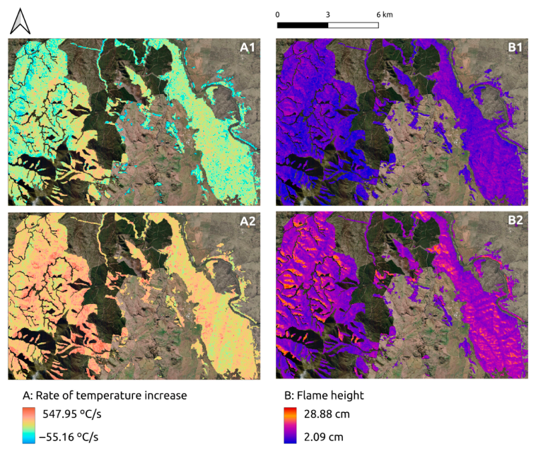
The spectral indices representing plant traits (see Section 2.5 and Section 3.5) were generated using the EnMAP imagery and were used as predictors in the selected models (see Section 2.5 and Section 3.6) to generate flammability maps (Figure 9). We used the EnMAP image from 5 April 2025 since the other two images contained clouds.
For the rate of temperature increase, laboratory values ranged between 69.52 and 262.50 °C/s, whereas Model A1 produced a wider range (−55.16 to 398.41 °C/s) with a mean of 127.73 °C/s (Table 7), partially overlapping the observed domain but including non-physical negative values, which are impossible by definition; these arise from the linear regression structure and the combination of coefficients and predictor values used during mapping. Model A1 also displayed overestimation at the upper end. Model A2 showed an even stronger shift towards higher values (155.24 to 547.95 °C/s; mean = 283.84 °C/s), exceeding the experimental range in both mean and maximum values, indicating systematic overestimation.
For flame height, laboratory values ranged from 7.41 to 13.47 cm. Model B1 (2.09 to 15.32 cm; mean = 9.30 cm, Table 7) largely overlapped the observed range, although it slightly underestimated minimum values. Model B2 (5.80 to 28.88 cm; mean = 12.63 cm, Table 7) better captured the central tendency but overestimated the upper range.
Overall, flame height models showed closer agreement with experimental observations, whereas rate of temperature increase models exhibited greater extrapolation beyond the observed range.

4. Discussion

Relationships between spectral properties and plant traits, and between plant traits and flammability are well documented [23,24,33,34]. This study integrated these two fields, establishing the relationships as a first attempt to propose a new protocol for developing fuel flammability maps based on fire-traits. Data was aggregated at plot level by its relative coverage to represent the information closer to an optical satellite, and flammability maps were modelled based on those relationships. This represents a feasibility study aimed at assessing the potential of this integrated approach for large-scale applications.

4.1. Reflectance Spectra, Plant Traits and Relationships

The samples exhibited the expected spectral patterns for each fuel type (live eucalypt, dead eucalypt, and grass), making them distinguishable through laboratory spectrometry, and hence in the EnMAP imagery.
Regarding the traits, the similarity in lLMA between live and dead eucalypt leaves indicates that structural properties are largely preserved after senescence. Eucalypts exhibited higher LMA and carbon content overall, consistent with global analyses showing that woody plants tend to have higher carbon concentrations than herbaceous species across tissues, including leaves [44]. In contrast, herbaceous plants such as grasses prioritize rapid growth and turnover, an evolutionary strategy associated with lower lignin and carbon investment. Instead, grasses rely more on structural carbohydrates (cellulose and hemicellulose) for support, which explains their higher average cellulose content [45,46].
It is also important to note that LA, used to calculate LMA, was measured at the whole-plant level in grasses, as separating leaves from stems was not feasible, and the entire plant represents the functional photosynthetic unit. This approach may increase variability in LMA estimates and complicate direct comparisons with eucalypt leaves. Few studies address LA measurement in grasses; among them, [47] recommends measuring only the lamina, although the appropriate method ultimately depends on the research objectives.
The quantification of biochemical traits such as carbon and cellulose relies on relatively complex laboratory protocols, including sample preparation, chemical extraction, and specialised instrumentation. This requirement may limit the reproducibility of the approach in contexts where such facilities are not available. However, the objective of this study was not to promote the use of specific traits, but to establish a general framework, within which alternative traits, potentially easier to measure or more widely available, can be incorporated depending on the study system and available resources.
From a remote sensing perspective, these structural and biochemical differences should be detectable in the spectral domain, as reflectance integrates multiple plant properties. Our results show that eucalypt reflectance had strong sensitivity to carbon content across the 600–1900 nm range, indicating that EnMAP imagery can capture spatial variation in key plant traits, fulfilling one of the main objectives of this study.
However, these results should be interpreted with caution. The relatively small sample size and limited temporal coverage restrict the ability to capture seasonal and spatial variability. Leaf functional traits and their corresponding optical properties are not static; they change significantly over a leaf’s lifespan and across seasons [48]. Expanding the dataset across multiple seasons and additional sites (in the case of the eucalypt forests, including more species) would likely improve model robustness and generalization.

4.2. Combustion Experiments

A new method for burning vegetation fuels (leaves and grasses) was used in this study, offering a simple, affordable, and reproducible approach. Flammability can be evaluated at different scales: leaf-level methods are among the most common due to their simplicity [16]. For instance, [18] proposed a methodology combining a moisture analyzer and a mass loss calorimeter, tested with plants [49] and landscape scales [50], although it requires a higher radiant heat flux (50 kW/m2). Shoot-level experiments are also widely used [51,52]. Whole-plant experiments, such as those proposed by [20], better capture plant architecture and often produce results closer to field conditions. However, sample collection and manipulation in these approaches are substantially more complex. Ultimately, some form of modelling is always required to upscale any of these measurements to landscape-scale applications [27].
Here, combustion was examined at the leaf level for eucalypts and at the whole-individual level for grasses. Although simpler than calorimeters or epiradiators, the experimental setup produced consistent and repeatable results, aided by the use of five replicates per sample, which helped minimise individual measurement errors. However, because samples were oven-dried prior to combustion, this method does not account for water-related plant traits, and instead characterises flammability primarily driven by structural and chemical properties.
For eucalypts, aggregating live and dead leaves at the plot level represents a first step toward scalability. This approach implicitly assumes additive flammability, meaning that the flammability of a mixture can be predicted simply by averaging the flammability of its constituent fuels. Nevertheless, non-additive effects may arise from emergent physicochemical interactions among fuels [27,29,53]. An exception is maximum temperature, which has sometimes shown additive behaviour, suggesting that this metric may be more predictable by averaging species contributions. In contrast, the grass protocol, where mixed shoots were combined in their field proportions, accounts for these non-additive effects and more closely represents real fuelbed composition. As a result, flammability values for eucalypts may under- or overestimate the true combined behaviour of mixed fuels, whereas grass values should better reflect field conditions.
Some flammability metrics commonly used in combustion research, such as peak heat release rate [50,54] or mass-loss rate [29], cannot be measured with this device. However, the rate of temperature increase used here reflects the rapid energy release during combustion, correlates with combustibility, and may serve as a practical proxy for peak heat release rate [55]. Most metrics measured in this study (time to ignition, flaming duration, mass loss, rate of temperature increase, and flame height) are widely used [16,56] and collectively cover the four classical components of flammability (ignitability, sustainability, consumability, and combustibility).
Regarding the relationship between plant traits and flammability metrics, research has shown that while partial drying may slightly reduce light volatiles, the heavy chemical components that drive sustained combustion remain largely unaffected [22]. Therefore, this method does not alter the measured traits.
LMA has been widely used as a structural predictor, typically showing negative correlations with ignitability, and positive correlations with sustainability and consumability across species, including eucalypt leaves and litter [24,57,58]. Relationships with combustibility are more variable [24,57]. In our results, LMA was positively correlated with consumability and with two of the combustibility metrics (maximum temperature and rate of temperature increase), but negatively correlated with flame height, the third combustibility metric, matching previously reported patterns. In grasses, LMA was positively correlated with all flammability components [59], arguing that higher dry-matter investment increases ignition, combustion intensity, and total consumption. This aligns with our results in showing that LMA enhances combustion in grasses, although in our dataset sustainability (flaming duration) was the clearest expression of this pattern.
Regarding chemical traits, volatile organic compounds (VOCs) have been extensively studied for their relationship with flammability [23,24,60,61], whereas research on cellulose and carbon is more limited [61]; nevertheless, our findings suggest that these traits may be highly informative. We observed a strong negative correlation between carbon content and flame height in eucalypts, the strongest relationship detected in this study, which, to our knowledge, has not been previously documented. More broadly, increases in carbon, cellulose, and LMA were associated with shorter flame heights but higher temperatures and faster heating rates. This pattern suggests that denser, carbon-rich leaves may burn with shorter but hotter and more intense flames. We also found a strong negative correlation between cellulose and consumability (relative mass loss) in grasses, which stands out as the most notable relationship for this vegetation type. Notably, aggregating data from individual samples to the plot level strengthened most trait–flammability relationships (compare Figure 6 and Figure 7). Together, these considerations indicate that even with a simple device, flammability can be quantified in a robust and reproducible way that links plant traits.

4.3. Mapping Plant Trait Indices

Due to the limited dataset and the feasibility nature of this study, we applied a parametric empirical regression approach, directly correlating spectral indices (difference, simple ratio, and normalised difference indices) with plant traits. This approach assumes a direct relationship between traits and indices, although in reality such relationships are often more complex. These methods are widely used and straightforward to implement, but they generally suffer from poor generalizability [35,62].
Spectral regions sensitive to one trait often overlap with those of others, leading to convergence among plant traits. As a result, indices developed to predict a specific trait may also capture variation in correlated traits, making it difficult to isolate spectral indices uniquely representative of a single vegetation property. For example, carbon is present in cellulose, pigments, VOCs, and affects LMA, making it difficult to isolate spectrally. This issue would arise regardless of the method used to derive plant-trait indices from spectral data and therefore represents an inherent limitation of the overall approach, since these indices are later used as independent predictors in the flammability models.
Empirical methods such as PLSR, a linear, non-parametric technique for quantifying vegetation parameters, have been widely used to address collinearity and high-dimensional spectral datasets. Several studies have confirmed the feasibility of PLSR for estimating biophysical variables from hyperspectral data in grasslands [35,63], and for analyzing flammability parameters strongly correlated [64]. However, despite its advantages, PLSR still requires sufficiently large datasets to capture the variance of the traits being modeled [34,48]. In practice, robust PLSR models typically rely on sample sizes of around 100 observations or more, and it is not uncommon to use datasets exceeding 200 samples [34].
Non-linear non-parametric methods such as Artificial Neural Networks or Gaussian Process Regression have demonstrated strong predictive performance [35]. In addition, hybrid models that combine radiative transfer modelling (RTM) with machine learning algorithms have shown promising results for estimating a wide variety of plant biophysical and biochemical traits from hyperspectral data [35,37,65,66,67,68]. Hybrid RTM-based methods can leverage large synthetic datasets to overcome limitations in field sample size. However, implementing such approaches requires a fundamentally different modelling framework, including the generation and calibration of radiative transfer simulations and, in many cases, the use of transfer learning strategies. The objective of this feasibility study was to establish empirical links between spectral indices, vegetation traits, and flammability using a simple and transparent methodology, and to generate flammability maps.
Beyond the modelling framework, several sensor-related considerations must be addressed. First, the extent to which laboratory spectra translate to satellite conditions is critical. In this study, field campaigns were aligned with cloud-free satellite overpasses under stable illumination conditions, and the best available atmospherically corrected EnMAP image was selected to ensure consistency between field and satellite reflectance. Sampling plots were deliberately located in homogeneous areas to minimise this effect; however, when extrapolating results to larger regions, especially heterogeneous eucalypt forests, mixed pixels are unavoidable and may reduce model performance. More importantly, when scaling from laboratory to landscape, factors such as canopy architecture, multiple scattering, leaf orientation, and background effects can substantially modify the spectral signal observed by spaceborne sensors [69], reflecting the challenge of scaling from controlled laboratory measurements to complex real-world canopy conditions.
Second, the sensor availability could represent an additional constraint. The use of EnMAP imagery, a commercial satellite with on-demand acquisitions, currently limits the applicability of this approach as an operational tool. However, the planned launch of the European Space Agency’s hyperspectral mission CHIME (Copernicus Hyperspectral Imaging Mission for the Environment), with CHIME-A expected in 2028 and CHIME-B in 2030, will provide free and open-access data, potentially overcoming these limitations [70].

4.4. Flammability Models and Maps

In this study, individual flammability metrics were predicted from plant traits. For eucalypts, both the trait–spectral relationships and the flammability models showed moderate performance, supporting the feasibility of linking spectral information to flammability through plant traits, although with clear limitations. Grassland systems remain comparatively understudied, both in general ecology and specifically in flammability research [71]. In our case, grass flammability models displayed poor predictive performance and were not retained for spatial application. This likely reflects both limitations in the selected plant traits and the suitability of the flammability metrics used for grasses, suggesting that exploring alternative traits and flammability metrics may improve model performance in these systems.
Regarding ecological generalizability, this aspect remains limited at this stage. The dataset is constrained in sample size and in its spatial and temporal coverage, and therefore, the results should not be extrapolated beyond the conditions under which the models were developed. This limitation is particularly relevant for grasslands, given their high variability and the lower model performance observed. Even for eucalypt systems, further validation across broader environmental gradients would be required before generalization.
Other approaches linking plant traits with flammability have combined several combustion components [16] or used Principal Component Analysis (PCA) to create composite flammability gradients [59,72,73,74]. Given the multivariate nature of flammability, integrated modelling strategies may better capture complex interactions among plant traits, combustion processes, and spectral properties.
The flammability maps developed here should not be interpreted as standalone fire risk maps. Instead, they represent a structural and biochemical component of flammability. In this context, they could be combined with independent moisture products to form a two-layer system, where this structural flammability is complemented by dynamic fuel moisture. Such an approach could provide a more complete representation of fire potential. Additionally, these maps may already be useful for prioritizing fuel treatments from a structural perspective, independent of short-term weather variability.
To our knowledge, few studies have produced flammability maps based on the classical definition of flammability as the ability of fuels to ignite and sustain combustion. One example is [50], which used laboratory-derived metrics (peak heat release rate) and kriging interpolation, achieving an RMSE of 24.15%. However, this approach relied primarily on interpolation rather than predictive modelling from remote sensing data, as models without spectral indices performed similarly to those incorporating Sentinel-2 or Moderate Resolution Imaging Spectroradiometer (MODIS)-derived indices. Furthermore, live fuel moisture content (LFMC) contributed substantially to model performance as a covariate in flammability estimation.
In contrast, operational products such as the Digital Earth Australia Fuel Moisture Content provide spatially continuous estimates of vegetation moisture at a 5-day resolution using RTM inversion of Sentinel-2 data, following approaches similar to the MODIS-based Australian Flammability Monitoring System (AFMS) [75]. While these products are widely used as proxies for flammability, they do not directly measure combustion properties. Recent work [76] has also shown that their performance is highly dependent on vegetation type and site homogeneity, with higher accuracy in grasslands (R2 = 0.83, RMSE = 32.45%) than in forests and shrublands (R2 = 0.43 and 0.21, respectively). This highlights the broader challenge of retrieving plant traits from remote sensing in heterogeneous landscapes. Overall, while earth observation techniques have expanded rapidly in recent decades, significant challenges remain in accurately linking spectral data to plant traits and flammability across ecosystems.
Finally, it is important to note that standard cross-validation approaches were not applied in this study due to the limited sample size. In small datasets, conventional methods such as K-fold cross-validation can produce highly variable and potentially overoptimistic estimates of model performance, driven by sampling noise, overfitting, and the risk of information leakage during model development. As a result, performance metrics may become sensitive to analytical choices and lack robustness. More rigorous validation strategies, such as nested cross-validation or independent train/test splits, require larger datasets or a sufficient number of independent observations to be reliable [77,78].

4.5. Future Research Directions

The limitations identified throughout this study highlight several directions for future research. First, expanding the number of study sites and conducting field campaigns across an entire growing season would allow a fuller representation of vegetation variability, improving both spectral–trait relationships and flammability modelling. The inclusion of additional plant traits with known relevance for flammability, such as leaf area, leaf area index (LAI), and VOCs [23,24,61,72] would also likely strengthen model performance.
Secondly, improving the combustion setup, particularly for shoot-level measurements by increasing heat flux, would help better simulate natural fuel structures and energy transfer, and could enable experiments without pre-drying, thereby allowing the inclusion of water-related traits.
Third, exploring alternative approaches for estimating plant traits from spectral data, such as PLSR or hybrid RTM-based models. Although the empirical regression approach used here is suitable for a feasibility study, more advanced methods could improve robustness and transferability. Given the scope of this work, we adopted a parsimonious approach that allows direct interpretation of trait–spectral relationships. While this method has known limitations in terms of generalization and sensitivity to confounding factors, it remains widely used and appropriate for exploratory analyses.
Lastly, future studies should incorporate independent validation datasets to evaluate predictive performance and assess model generalization beyond the conditions of this study.

5. Conclusions

This study demonstrates the feasibility of linking spectral information, plant traits, and flammability metrics within a coherent framework capable of producing spatially explicit estimates of flammability. Laboratory spectra effectively distinguished fuel types and captured variability in plant traits, enabling the derivation of spectral indices and the prediction of vegetation properties. Structural and biochemical traits explained meaningful variation in eucalypt flammability, particularly for combustibility metrics such as the rate of temperature increase and flame height, and these relationships translated into spatially coherent maps. In contrast, grasses exhibited weaker and less consistent trait–flammability relationships, resulting in low model performance. Consequently, grass flammability models were not considered suitable for spatial application, highlighting the need for improved trait selection and more appropriate flammability metrics in these systems.
The combustion protocol adopted here isolates flammability driven by structural and biochemical properties while maintaining moisture under controlled conditions. As a result, the derived maps represent the structural and biochemical drivers of combustion rather than operational fire risk. These products should therefore be interpreted as complementary layers that can be integrated with independent fuel moisture information to support more comprehensive assessments of fire behaviour.
Overall, this work provides a novel framework for trait-based flammability mapping using hyperspectral data. While the approach shows clear potential, its generalisation requires larger datasets, broader environmental coverage, improved plant trait retrieval methods, and independent validation. Future work should also explore non-linear modelling frameworks to better capture the complexity of vegetation flammability across ecosystems.

Supplementary Materials

The following supporting information can be downloaded at: https://www.mdpi.com/article/10.3390/rs18101546/s1, Supplementary Table S1 provides the list of sampled plant species and their percentage cover across sites, paddocks, plots, and fuel types; Table S2 presents the fractional cover of each species and litter component; Figure S1 shows the study-site vegetation map; Figures S2–S6 show the measured vegetation traits across dates and plots; Tables S3–S4 summarize the statistical tests and replicate-level variability of the combustion experiments; Figure S7 presents the correlation structure among flammability metrics; Figure S8 displays the relationship between vegetation traits and flammability metrics for eucalypt and grass samples.

Author Contributions

Conceptualization, A.V. and N.Y.; methodology, A.V., N.Y., M.I., M.Y., and J.M.; software, A.V.; validation, A.V.; formal analysis, A.V.; investigation, A.V.; resources, N.Y. and M.Y.; data curation, A.V. and N.Y.; writing—original draft preparation, A.V.; writing—review and editing, N.Y., M.I. and J.M.; visualization, A.V.; supervision, N.Y., I.d.l.C., and J.M.; project administration, N.Y.; funding acquisition, N.Y., I.d.l.C. and J.M. All authors have read and agreed to the published version of the manuscript.

Funding

This research was funded by Comunidad de Madrid Industrial Doctorate Programme 2022, grant number IND2022 BIO23597 and Agencia Española de Investigación, Ministerio de Ciencia, Innovación y Universidades, grant number ZEGIADAPT PID2023-146599OR-C51.

Data Availability Statement

Dataset available on request from the authors. The raw data supporting the conclusions of this article will be made available by the authors on request.

Acknowledgments

Torsten Riedlinger and Nicole Pinnel, from DLR for providing the EnMAP data; ACT Parks and Conservation Service for providing access to the LCCR site; Eric Hay from ANU for assistance during the field campaigns, Nick Wilson from ANU for advice on thermal camera operation, Andrew Sullivan from CSIRO for guidance on the combustion experiments, and Matt Sutton from ANU for constructing the metallic mesh device; Katie and Duncan for their hospitality.

Conflicts of Interest

The authors declare no conflict of interest.

Appendix A. Combustion Experiments

For the leaf setup, leaf samples were individually positioned on a metal grid placed 5 cm above a Bunsen burner (Figure A1C). For the grasses, following [48], a metallic rectangular mesh container (10 × 10 × 40 cm) was crafted to contain the samples while allowing air flow (Figure A1B). The samples were placed on the bottom of the mesh container against the same grid used for the leaf samples. The burner was ignited first and adjusted until the flame reached above the grid level. The leaf sample or the metallic box with the grass sample was then exposed to the flame until ignition occurred, at which point the burner was turned off.
Figure A1. Combustion experiment setup (A), grasses on the mesh container (B) and burning leaf on top of the metallic grid (C).
Remotesensing 18 01546 g0a1
Each experiment was recorded simultaneously using a thermal camera (Optris Xi 400) and a high-resolution video camera (Sony HDR-CX405) to extract flammability metrics (Table 1). A measuring tape was attached to a non-reflective black plate used as a background to avoid interference with the thermal camera, while allowing us to record flame height. To minimise airflow interference from outside the experiment, the air extractor was turned off during each experiment and reactivated between trials to ensure air circulation in the room. The flame temperature of the Bunsen burner remained stable during the experiments, consistently reaching approximately 150 °C. The temperature and humidity in the laboratory during the experiments ranged from 19 to 22 °C and from 41 to 57%, respectively.
Five replicates were conducted for each sample, ensuring robust results despite the small sample size. All vegetation samples were previously oven-dried at 40 °C for four days before the flammability experiments, in order to facilitate the combustion [20,49]. The remaining vegetative material was analysed to determine the moisture content at the time of combustion. It is important to note that this does not represent the fuel moisture content (FMC) of fresh samples, but rather the residual moisture content following partial drying, and immediately before the combustion experiments. This additional measurement allows for the reproducibility of the experimental conditions. Grasses were mixed at the plot level according to their relative coverage (see Section 2.2). This approach was chosen to better reflect real-world conditions and to account for potential non-additive effects among species during combustion.
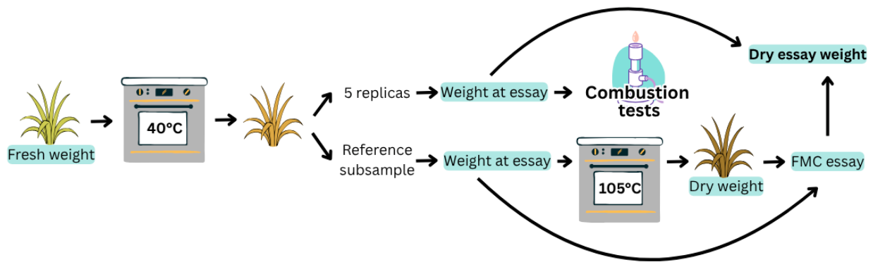
Nine flammability metrics were measured in these experiments during the combustion experiments. Time to ignition refers to the time it takes for the sample to ignite after being placed above the flame, either as a single leaf or as grasses in a metallic prism. Flaming duration is defined as the time from ignition until the flame is completely extinguished. Normalisation was performed by dividing each value by the dry mass of the sample (Figure A2) to obtain the normalised time to ignition and the normalised flaming duration. In cases where multiple ignitions occurred, the total duration includes all burning events until the final extinction. These time-based variables were extracted from video recordings, which provided precise timestamps. Mass loss was calculated as the difference between the sample’s initial and final weight, recorded directly during the experiment, while relative mass loss was calculated by dividing by the initial weight of the sample. Maximum temperature was defined as the highest temperature achieved during the combustion, and was recorded by the thermal camera as the highest value within the flame area of the sample during combustion (see Figure A2). The rate of temperature increase was calculated as the derivative of the temperature curve at the initial phase of combustion, corresponding to the period of rapid heating. Flame height refers to the maximum vertical extent of the flame during combustion. It was measured only for leaf samples and was also derived from the video footage.
Figure A2. Schematic diagram illustrating the calculation of dry weight at the time of the experiment. Blue highlights indicate parameters measured during the experiment.
Remotesensing 18 01546 g0a2
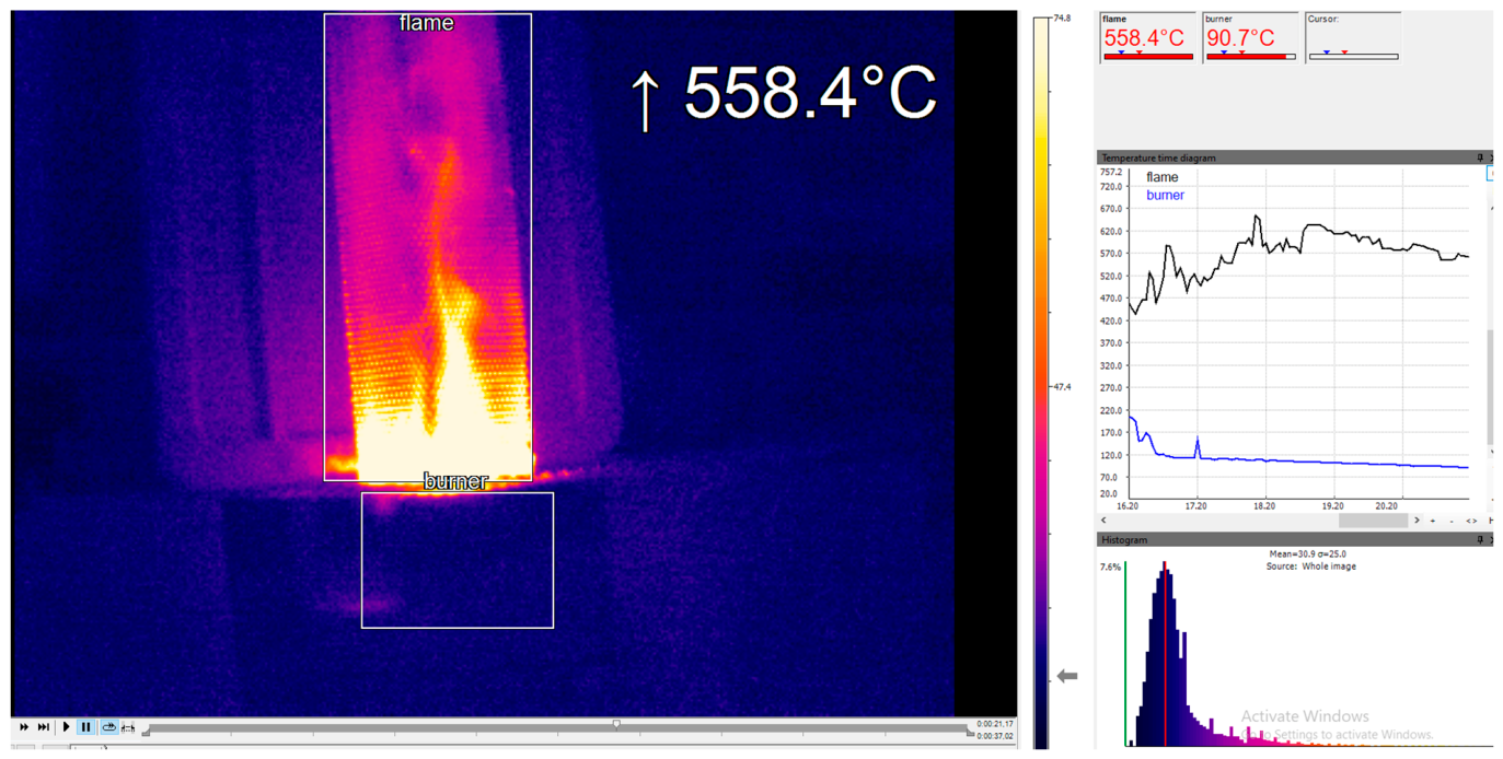
Figure A3. Screenshot of the PIX Connect 3.24.3127.0 software during a grass combustion. The box labelled “Flame” indicates the area where the highest pixel value was selected during combustion to determine the maximum temperature; at the moment shown, the maximum temperature recorded in this box was 558.41 °C. The “Burner” box marks the region corresponding to the Bunsen burner flame, used to monitor burner stability throughout the experiment. The right panel displays the maximum temperature for both boxes, temperature trends over time, and a histogram of recorded temperatures.
Remotesensing 18 01546 g0a3

References

  1. Glasspool, I.J.; Gastaldo, R.A. Don’t Mind the “Charcoal Gap”: A Reassessment of Devonian Wildfire. Geology 2024, 52, 846–850. [Google Scholar] [CrossRef]
  2. Pausas, J.G.; Keeley, J.E.; Bond, W.J. The Role of Fire on Earth. BioScience 2025, 75, biaf132. [Google Scholar] [CrossRef]
  3. McLauchlan, K.K.; Higuera, P.E.; Miesel, J.; Rogers, B.M.; Schweitzer, J.; Shuman, J.K.; Tepley, A.J.; Varner, J.M.; Veblen, T.T.; Adalsteinsson, S.A.; et al. Fire as a Fundamental Ecological Process: Research Advances and Frontiers. J. Ecol. 2020, 108, 2047–2069. [Google Scholar] [CrossRef]
  4. Pereira, P.; Bogunovic, I.; Zhao, W.; Barcelo, D. Short-Term Effect of Wildfires and Prescribed Fires on Ecosystem Services. Curr. Opin. Environ. Sci. Health 2021, 22, 100266. [Google Scholar] [CrossRef]
  5. Morgan, G.W.; Tolhurst, K.G.; Poynter, M.W.; Cooper, N.; McGuffog, T.; Ryan, R.; Wouters, M.A.; Stephens, N.; Black, P.; Sheehan, D.; et al. Prescribed Burning in South-Eastern Australia: History and Future Directions. Aust. For. 2020, 83, 4–28. [Google Scholar] [CrossRef]
  6. Kelley, D.I.; Burton, C.; Di Giuseppe, F.; Jones, M.W.; Barbosa, M.L.F.; Brambleby, E.; McNorton, J.R.; Liu, Z.; Bradley, A.S.I.; Blackford, K.; et al. State of Wildfires 2024–2025. Earth Syst. Sci. Data 2025, 17, 5377–5488. [Google Scholar] [CrossRef]
  7. Liu, Z.; Ballantyne, A.P.; Cooper, L.A. Biophysical Feedback of Global Forest Fires on Surface Temperature. Nat. Commun. 2019, 10, 214. [Google Scholar] [CrossRef] [PubMed]
  8. Tyukavina, A.; Potapov, P.; Hansen, M.C.; Pickens, A.H.; Stehman, S.V.; Turubanova, S.; Parker, D.; Zalles, V.; Lima, A.; Kommareddy, I.; et al. Global Trends of Forest Loss Due to Fire From 2001 to 2019. Front. Remote Sens. 2022, 3, 825190. [Google Scholar] [CrossRef]
  9. Arrogante-Funes, F.; Aguado, I.; Chuvieco, E. Global Assessment and Mapping of Ecological Vulnerability to Wildfires. Nat. Hazards Earth Syst. Sci. 2022, 22, 2981–3003. [Google Scholar] [CrossRef]
  10. Xu, R.; Yu, P.; Abramson, M.; Johnston, F.; Samet, J.; Bell, M.; Haines, A.; Ebi, K.; Li, S.; Guo, Y. Wildfires, Global Climate Change, and Human Health. N. Engl. J. Med. 2020, 383, 2173–2181. [Google Scholar] [CrossRef]
  11. Johnston, F.H.; Henderson, S.B.; Chen, Y.; Randerson, J.T.; Marlier, M.; DeFries, R.S.; Kinney, P.; Bowman, D.M.J.S.; Brauer, M. Estimated Global Mortality Attributable to Smoke from Landscape Fires. Environ. Health Perspect. 2012, 120, 695–701. [Google Scholar] [CrossRef]
  12. Qiu, M.; Li, J.; Gould, C.F.; Jing, R.; Kelp, M.; Childs, M.; Kiang, M.; Heft-Neal, S.; Diffenbaugh, N.; Burke, M. Mortality Burden from Wildfire Smoke Under Climate Change. 2024. Available online: http://www.nber.org/papers/w32307 (accessed on 16 October 2025).
  13. Meier, S.; Elliott, R.J.R.; Strobl, E. The Regional Economic Impact of Wildfires: Evidence from Southern Europe. J. Environ. Econ. Manag. 2023, 118, 102787. [Google Scholar] [CrossRef]
  14. Anderson, H.E. Forest Fuel Ignitibility. Fire Technol. 1970, 6, 312–319. [Google Scholar] [CrossRef]
  15. Tumino, B.J.; Duff, T.J.; Goodger, J.Q.D.; Cawson, J.G. Plant Traits Linked to Field-Scale Flammability Metrics in Prescribed Burns in Eucalyptus Forest. PLoS ONE 2019, 14, e0221403. [Google Scholar] [CrossRef]
  16. Jian, M.; Jian, Y.; Zeng, H.; Cao, D.; Cui, X. Current Status and Prospects of Plant Flammability Measurements. Fire 2024, 7, 266. [Google Scholar] [CrossRef]
  17. Martin, R.E.; Gordon, D.A.; Gutierrez, M.E.; Lee, D.S.; Molina, D.M.; Schroeder, R.A.; Sapsis, D.B.; Stephens, S.L. Assessing the Flammability of Domestic and Wildland Vegetation. In Proceedings of the 12th Conference of Fire and Forest Meteorology, Jekyll Island, GA, USA, 26–28 October 1993; Society of American Foresters: Bethesda, MD, USA, 1993. [Google Scholar] [CrossRef]
  18. Madrigal, J.; Hernando, C.; Guijarro, M. A New Bench-Scale Methodology for Evaluating the Flammability of Live Forest Fuels. J. Fire Sci. 2013, 31, 131–142. [Google Scholar] [CrossRef]
  19. Celebrezze, J.V.; Boving, I.; Moritz, M.A. Tissue-Level Flammability Testing: A Review of Existing Methods and a Comparison of a Novel Hot Plate Design to an Epiradiator Design. Fire 2023, 6, 149. [Google Scholar] [CrossRef]
  20. Jaureguiberry, P.; Bertone, G.; Díaz, S. Device for the Standard Measurement of Shoot Flammability in the Field: Flammability Measurement in the Field. Austral Ecol. 2011, 36, 821–829. [Google Scholar] [CrossRef]
  21. Fuentes-Ramirez, A.; Veldman, J.W.; Holzapfel, C.; Moloney, K.A. Spreaders, Igniters, and Burning Shrubs: Plant Flammability Explains Novel Fire Dynamics in Grass-invaded Deserts. Ecol. Appl. 2016, 26, 2311–2322. [Google Scholar] [CrossRef]
  22. Hamamousse, N.; Mosbah, O.; Kaiss, A.; Boutchiche, H.; Chaib, F.; Hammane, Y.; Terrah, S.-M.; Sabi, F.-Z.; Clerc, J.-P.; Chikhaoui, A.; et al. Effect of Drying on the Ignitability and Combustibility of Pinus Halepensis Needles. Fire Saf. J. 2022, 127, 103505. [Google Scholar] [CrossRef]
  23. Popović, Z.; Bojović, S.; Marković, M.; Cerdà, A. Tree Species Flammability Based on Plant Traits: A Synthesis. Sci. Total Environ. 2021, 800, 149625. [Google Scholar] [CrossRef] [PubMed]
  24. Younes, N.; Yebra, M.; Boer, M.M.; Griebel, A.; Nolan, R.H. A Review of Leaf-Level Flammability Traits in Eucalypt Trees. Fire 2024, 7, 183. [Google Scholar] [CrossRef]
  25. Molina, J.R.; Martín, T.; Rodríguez Y Silva, F.; Herrera, M.Á. The Ignition Index Based on Flammability of Vegetation Improves Planning in the Wildland-Urban Interface: A Case Study in Southern Spain. Landsc. Urban Plan. 2017, 158, 129–138. [Google Scholar] [CrossRef]
  26. Molina, J.R.; Lora, A.; Prades, C.; Rodríguez, Y.; Silva, F. Roadside Vegetation Planning and Conservation: New Approach to Prevent and Mitigate Wildfires Based on Fire Ignition Potential. For. Ecol. Manag. 2019, 444, 163–173. [Google Scholar] [CrossRef]
  27. Schwilk, D.W.; Alam, M.A.; Gill, N.; Murray, B.R.; Nolan, R.H.; Ondei, S.; Perry, G.L.W.; Smith, A.M.S.; Bowman, D.M.J.S.; Fidelis, A.; et al. From Plant Traits to Fire Behavior: Scaling Issues in Flammability Studies. Am. J. Bot. 2025, 112, e70040. [Google Scholar] [CrossRef]
  28. Van Altena, C.; van Logtestijn, R.; Cornwell, W.; Cornelissen, J. Species Composition and Fire: Non-Additive Mixture Effects on Ground Fuel Flammability. Front. Plant Sci. 2012, 3. [Google Scholar] [CrossRef]
  29. Simpson, K.J.; Ripley, B.S.; Christin, P.; Belcher, C.M.; Lehmann, C.E.R.; Thomas, G.H.; Osborne, C.P. Determinants of Flammability in Savanna Grass Species. J. Ecol. 2016, 104, 138–148. [Google Scholar] [CrossRef]
  30. Jolly, W.M.; Johnson, D.M. Pyro-Ecophysiology: Shifting the Paradigm of Live Wildland Fuel Research. Fire 2018, 1, 8. [Google Scholar] [CrossRef]
  31. Resco De Dios, V. Plant-Fire Interactions: Applying Ecophysiology to Wildfire Management; Managing Forest Ecosystems; Springer International Publishing: Cham, Switzerland, 2020; Volume 36, ISBN 978-3-030-41191-6. [Google Scholar]
  32. Dickman, L.T.; Jonko, A.K.; Linn, R.R.; Altintas, I.; Atchley, A.L.; Bär, A.; Collins, A.D.; Dupuy, J.; Gallagher, M.R.; Hiers, J.K.; et al. Integrating Plant Physiology into Simulation of Fire Behavior and Effects. New Phytol. 2023, 238, 952–970. [Google Scholar] [CrossRef] [PubMed]
  33. Kothari, S.; Beauchamp-Rioux, R.; Blanchard, F.; Crofts, A.L.; Girard, A.; Guilbeault-Mayers, X.; Hacker, P.W.; Pardo, J.; Schweiger, A.K.; Demers-Thibeault, S.; et al. Predicting Leaf Traits across Functional Groups Using Reflectance Spectroscopy. New Phytol. 2023, 238, 549–566. [Google Scholar] [CrossRef]
  34. Burnett, A.C.; Anderson, J.; Davidson, K.J.; Ely, K.S.; Lamour, J.; Li, Q.; Morrison, B.D.; Yang, D.; Rogers, A.; Serbin, S.P. A Best-Practice Guide to Predicting Plant Traits from Leaf-Level Hyperspectral Data Using Partial Least Squares Regression. J. Exp. Bot. 2021, 72, 6175–6189. [Google Scholar] [CrossRef]
  35. Xie, R.; Darvishzadeh, R.; Skidmore, A.K.; Heurich, M.; Holzwarth, S.; Gara, T.W.; Reusen, I. Mapping Leaf Area Index in a Mixed Temperate Forest Using Fenix Airborne Hyperspectral Data and Gaussian Processes Regression. Int. J. Appl. Earth Obs. Geoinf. 2021, 95, 102242. [Google Scholar] [CrossRef]
  36. Singh, P.; Srivastava, P.K.; Jha, P.K.; Verrelst, J.; Singh, P.N.; Prasad, R. Retrieval of Crop Traits Using PROSAIL-Based Hybrid Radiative Transfer Model and EnMAP Hyperspectral Data. Int. J. Appl. Earth Obs. Geoinf. 2025, 143, 104769. [Google Scholar] [CrossRef]
  37. Farmonov, N.; Walden, S.; Martinée, E.; Lampei, C.; Schreiber, M.; Opgenoorth, L.; Rakotomalala, A.A.N.A.; Müller, T.; Farwig, N.; Pinkert, S.; et al. Optimizing Hybrid Models for Forest Leaf and Canopy Trait Mapping from EnMAP Hyperspectral Data with Limited Field Samples. Sci. Remote Sens. 2025, 12, 100253. [Google Scholar] [CrossRef]
  38. Camilleri, P.; Healy, C.; Macdonald, E.; Nicholls, S.; Sykes, J.; Winkworth, G.; Woodward, M. Recovery from Bushfires: The Experience of the 2003 Canberra Bushfires Three Years After. Australas. J. Paramed. 2010, 8, 1–15. [Google Scholar] [CrossRef]
  39. Matthews, S. Dead Fuel Moisture Research: 1991–2012. Int. J. Wildland Fire 2014, 23, 78. [Google Scholar] [CrossRef]
  40. Cain, S.; Younes, N. Cellulose Extraction and Quantification from Eucalyptus Leaves in the Laboratory. Protoc. Exch. 2024. [Google Scholar] [CrossRef]
  41. Younes, N.; Cain, S. Carbon and Nitrogen Nutrient Analysis of Eucalyptus Leaves. Protoc. Exch. 2024. [Google Scholar] [CrossRef]
  42. Viñuales, A.; Younes, N. Protocol for Conducting Combustion Experiments to Measure Grass Flammability. Protoc. Exch. 2026. [Google Scholar] [CrossRef]
  43. Guanter, L.; Kaufmann, H.; Segl, K.; Foerster, S.; Rogass, C.; Chabrillat, S.; Kuester, T.; Hollstein, A.; Rossner, G.; Chlebek, C.; et al. The EnMAP Spaceborne Imaging Spectroscopy Mission for Earth Observation. Remote Sens. 2015, 7, 8830–8857. [Google Scholar] [CrossRef]
  44. Ma, S.; He, F.; Tian, D.; Zou, D.; Yan, Z.; Yang, Y.; Zhou, T.; Huang, K.; Shen, H.; Fang, J. Variations and Determinants of Carbon Content in Plants: A Global Synthesis. Biogeosciences 2018, 15, 693–702. [Google Scholar] [CrossRef]
  45. Ma, W.; Zhai, L.; Pivovaroff, A.; Shuman, J.; Buotte, P.; Ding, J.; Christoffersen, B.; Knox, R.; Moritz, M.; Fisher, R.A.; et al. Assessing Climate Change Impacts on Live Fuel Moisture and Wildfire Risk Using a Hydrodynamic Vegetation Model. Biogeosciences 2021, 18, 4005–4020. [Google Scholar] [CrossRef]
  46. Armstrong, D.G.; Cook, H.; Thomas, B. The Lignin and Cellulose Contents of Certain Grassland Species at Different Stages of Growth. J. Agric. Sci. 1950, 40, 93–99. [Google Scholar] [CrossRef]
  47. Pérez-Harguindeguy, N.; Díaz, S.; Garnier, E.; Lavorel, S.; Poorter, H.; Jaureguiberry, P.; Bret-Harte, M.S.; Cornwell, W.K.; Craine, J.M.; Gurvich, D.E.; et al. New Handbook for Standardised Measurement of Plant Functional Traits Worldwide. Aust. J. Bot. 2013, 61, 167–234. [Google Scholar] [CrossRef]
  48. Serbin, S.P.; Townsend, P.A. Scaling Functional Traits from Leaves to Canopies. In Remote Sensing of Plant Biodiversity; Cavender-Bares, J., Gamon, J.A., Townsend, P.A., Eds.; Springer International Publishing: Cham, Switzerland, 2020; pp. 43–82. ISBN 978-3-030-33156-6. [Google Scholar]
  49. Della Rocca, G.; Danti, R.; Hernando, C.; Guijarro, M.; Michelozzi, M.; Carrillo, C.; Madrigal, J. Terpenoid Accumulation Links Plant Health and Flammability in the Cypress-Bark Canker Pathosystem. Forests 2020, 11, 651. [Google Scholar] [CrossRef]
  50. Viñuales, A.; Montes, F.; Guijarro, M.; Gómez, C.; Calle, I.D.L.; Madrigal, J. Real-Time Assessment of Live Forest Fuel Moisture Content and Flammability by Using Space-Time Universal Kriging. Ecol. Model. 2024, 498, 110867. [Google Scholar] [CrossRef]
  51. Wyse, S.V.; Perry, G.L.W.; O’Connell, D.M.; Holland, P.S.; Wright, M.J.; Hosted, C.L.; Whitelock, S.L.; Geary, I.J.; Maurin, K.J.L.; Curran, T.J. A Quantitative Assessment of Shoot Flammability for 60 Tree and Shrub Species Supports Rankings Based on Expert Opinion. Int. J. Wildland Fire 2016, 25, 466. [Google Scholar] [CrossRef]
  52. Alam, M.A.; Wyse, S.V.; Buckley, H.L.; Perry, G.L.W.; Sullivan, J.J.; Mason, N.W.H.; Buxton, R.; Richardson, S.J.; Curran, T.J. Shoot Flammability Is Decoupled from Leaf Flammability, but Controlled by Leaf Functional Traits. J. Ecol. 2020, 108, 641–653. [Google Scholar] [CrossRef]
  53. Della Rocca, G.; Danti, R.; Hernando, C.; Guijarro, M.; Madrigal, J. Flammability of Two Mediterranean Mixed Forests: Study of the Non-Additive Effect of Fuel Mixtures in Laboratory. Front. Plant Sci. 2018, 9, 825. [Google Scholar] [CrossRef]
  54. Madrigal, J.; Guijarro, M.; Hernando, C.; Díez, C.; Marino, E. Estimation of Peak Heat Release Rate of a Forest Fuel Bed in Outdoor Laboratory Conditions. J. Fire Sci. 2011, 29, 53–70. [Google Scholar] [CrossRef]
  55. Madrigal, J.; Marino, E.; Guijarro, M.; Hernando, C.; Díez, C. Evaluation of the Flammability of Gorse (Ulex europaeus L.) Managed by Prescribed Burning. Ann. For. Sci. 2012, 69, 387–397. [Google Scholar] [CrossRef]
  56. Ocampo-Zuleta, K.; Pausas, J.G.; Paula, S. FLAMITS: A Global Database of Plant Flammability Traits. Glob. Ecol. Biogeogr. 2023, 33, 412–425. [Google Scholar] [CrossRef]
  57. Burton, J.E.; Cawson, J.G.; Filkov, A.I.; Penman, T.D. Leaf Traits Predict Global Patterns in the Structure and Flammability of Forest Litter Beds. J. Ecol. 2021, 109, 1344–1355. [Google Scholar] [CrossRef]
  58. Grootemaat, S.; Wright, I.J.; Van Bodegom, P.M.; Cornelissen, J.H.C.; Cornwell, W.K. Burn or Rot: Leaf Traits Explain Why Flammability and Decomposability Are Decoupled across Species. Funct. Ecol. 2015, 29, 1486–1497. [Google Scholar] [CrossRef]
  59. Padullés Cubino, J.; Buckley, H.L.; Day, N.J.; Pieper, R.; Curran, T.J. Community-level Flammability Declines over 25 Years of Plant Invasion in Grasslands. J. Ecol. 2018, 106, 1582–1594. [Google Scholar] [CrossRef]
  60. Ganteaume, A.; Romero, B.; Ormeño, E.; Lecareux, C.; Fernandez, C. Does the Temporal Variation of Leaf Terpene and Moisture Content Trigger Leaf Flammability over Time? Int. J. Wildland Fire 2025, 34, WF24190. [Google Scholar] [CrossRef]
  61. Guerrero, F.; Espinoza, L.; Carmona, C.; Blackhall, M.; Quintero, C.; Ocampo-Zuleta, K.; Paula, S.; Madrigal, J.; Guijarro, M.; Carrasco, Y.; et al. Unraveling the Chemistry of Plant Flammability: Exploring the Role of Volatile Secondary Metabolites beyond Terpenes. For. Ecol. Manag. 2024, 572, 122269. [Google Scholar] [CrossRef]
  62. Broge, N.H.; Leblanc, E. Comparing Prediction Power and Stability of Broadband and Hyperspectral Vegetation Indices for Estimation of Green Leaf Area Index and Canopy Chlorophyll Density. Remote Sens. Environ. 2001, 76, 156–172. [Google Scholar] [CrossRef]
  63. Darvishzadeh, R.; Atzberger, C.; Skidmore, A.K. Hyperspectral Vegetation Indices for Estimation of Leaf Area Index. In ISPRS Commission VII Symposium 2006: Remote Sensing: From Pixels to Processes; International Institute for Geo-Information Science and Earth Observation: Enschede, The Netherlands, 2006. [Google Scholar]
  64. Della Rocca, G.; Madrigal, J.; Marchi, E.; Michelozzi, M.; Moya, B.; Danti, R. Relevance of Terpenoids on Flammability of Mediterranean Species: An Experimental Approach at a Low Radiant Heat Flux. IForest Biogeosci. For. 2017, 10, 766–775. [Google Scholar] [CrossRef]
  65. Ji, F.; Li, F.; Dashti, H.; Hao, D.; Townsend, P.A.; Zheng, T.; You, H.; Chen, M. Leveraging Transfer Learning and Leaf Spectroscopy for Leaf Trait Prediction with Broad Spatial, Species, and Temporal Applicability. Remote Sens. Environ. 2025, 326, 114818. [Google Scholar] [CrossRef]
  66. Tagliabue, G.; Boschetti, M.; Bramati, G.; Candiani, G.; Colombo, R.; Nutini, F.; Pompilio, L.; Rivera-Caicedo, J.P.; Rossi, M.; Rossini, M.; et al. Hybrid Retrieval of Crop Traits from Multi-Temporal PRISMA Hyperspectral Imagery. ISPRS J. Photogramm. Remote Sens. 2022, 187, 362–377. [Google Scholar] [CrossRef]
  67. Ali, A.M.; Darvishzadeh, R.; Skidmore, A.; Gara, T.W.; Heurich, M. Machine Learning Methods’ Performance in Radiative Transfer Model Inversion to Retrieve Plant Traits from Sentinel-2 Data of a Mixed Mountain Forest. Int. J. Digit. Earth 2021, 14, 106–120. [Google Scholar] [CrossRef]
  68. Wocher, M.; Berger, K.; Verrelst, J.; Hank, T. Retrieval of Carbon Content and Biomass from Hyperspectral Imagery over Cultivated Areas. ISPRS J. Photogramm. Remote Sens. 2022, 193, 104–114. [Google Scholar] [CrossRef]
  69. Cavender-Bares, J.; Gamon, J.A.; Townsend, P.A. (Eds.) Remote Sensing of Plant Biodiversity; Springer International Publishing: Cham, Switzerland, 2020; ISBN 978-3-030-33156-6. [Google Scholar]
  70. Nieke, J.; Despoisse, L.; Gabriele, A.; Weber, H.; Strese, H.; Ghasemi, N.; Gascon, F.; Alonso, K.; Boccia, V.; Tsonevska, B.; et al. The Copernicus Hyperspectral Imaging Mission for the Environment (CHIME): An Overview of Its Mission, System and Planning Status. In Proceedings of the Sensors, Systems, and Next-Generation Satellites XXVII, Amsterdam, The Netherlands, 3–6 September 2023; Amsterdam, The Netherlands, Kimura, T., Babu, S.R., Hélière, A., Eds.; SPIE: Amsterdam, The Netherlands, 2023; p. 7. [Google Scholar]
  71. Li, Y.; Xiong, K.; Song, S.; Zhang, W. Realizing the Value of Grassland Ecosystem Services: Global Practice and Its Inspiration for the Karst Desertification Control Area. Front. Sustain. Food Syst. 2024, 7, 1240431. [Google Scholar] [CrossRef]
  72. Simha, A.; Coughlin, A.; Anderson, S.M.; DeLaMater, D.; Thayer, E.; Wong, R.J.; Wright, J.P. Form, Physiology, and Fire Response Explain Key Dimensions of Litter Flammability in Fire-adapted Longleaf Pine Savanna. New Phytol. 2025, 247, 2063–2073. [Google Scholar] [CrossRef] [PubMed]
  73. Boving, I.; Celebrezze, J.; Salladay, R.; Ramirez, A.; Anderegg, L.D.L.; Moritz, M. Live Fuel Moisture and Water Potential Exhibit Differing Relationships with Leaf-level Flammability Thresholds. Funct. Ecol. 2023, 37, 2770–2785. [Google Scholar] [CrossRef]
  74. Sultana, N.; Macinnis-Ng, C.; Richardson, S.J.; Alam, M.A.; Cui, X.; Wyse, S.V.; Laughlin, D.C.; Seward, K.; Perry, G.L.W.; Curran, T.J. Testing Key Tenets of Pyro-ecophysiology: Indicators of Drought Response in Relation to Shoot Flammability. Am. J. Bot. 2025, 112, e70091. [Google Scholar] [CrossRef]
  75. Yebra, M.; Quan, X.; Riaño, D.; Rozas Larraondo, P.; Van Dijk, A.I.J.M.; Cary, G.J. A Fuel Moisture Content and Flammability Monitoring Methodology for Continental Australia Based on Optical Remote Sensing. Remote Sens. Environ. 2018, 212, 260–272. [Google Scholar] [CrossRef]
  76. Yebra, M.; Scortechini, G.; Younes, N.; Van Dijk, A.I.J.M. High-Resolution Monitoring of Live Fuel Moisture Content Across Australia. Remote Sens. 2026, 18, 1049. [Google Scholar] [CrossRef]
  77. Vabalas, A.; Gowen, E.; Poliakoff, E.; Casson, A.J. Machine Learning Algorithm Validation with a Limited Sample Size. PLoS ONE 2019, 14, e0224365. [Google Scholar] [CrossRef]
  78. Varoquaux, G. Cross-Validation Failure: Small Sample Sizes Lead to Large Error Bars. Neuroimage 2018, 180, 68–77. [Google Scholar] [CrossRef] [PubMed]
Figure 1. Australian Capital Territory (ACT) location (top); study sites (bottom left) and plot distribution (bottom right) in Spring Valley Farm (SVF) and the Lower Cotter Catchment Reserve (LCCR). Green circles represent sampling plots, while the red border in the SVF figure indicates paddock limits.
Remotesensing 18 01546 g001
Figure 2. Workflow diagram. Field samples collected during satellite overpasses were processed for spectroscopy, plant traits, and flammability, integrated into a dataset, and used to model relationships and produce flammability maps. LMA: Leaf Mass per Area; TI: time to ignition; NTI: normalised time to ignition; FD: flaming duration; NFD: normalised flaming duration; ML: mass loss; RML: relative mass loss; MT: maximum temperature; RTI: rate of temperature increase; FH: flame height.
Remotesensing 18 01546 g002
Figure 3. Mean spectral signatures (solid lines) of live and dead eucalypt and grass samples obtained during this experiment. Shaded coloured areas represent ±1 standard deviation. Gray areas represent water absorption features.
Remotesensing 18 01546 g003
Figure 4. Boxplot of the flammability metrics for live and dead eucalypt and grass samples. (Subfigures A,B): Ignitability, represented by (A) time to ignition (TI, s) and (B) normalised time to ignition (NTI, s/g); (Subfigures C,D): sustainability, represented by (C) flaming duration (FD, s) and (D) normalised flaming duration (NFD, s/g); (Subfigures E,F): consumability, represented by (E) mass loss (ML, g) and (F) relative mass loss (RML); and (Subfigures GI): combustibility, represented by (G) maximum temperature (MT, °C), (H) rate of temperature increase (RTI, °C/s), and (I) flame height (FH, cm). Colours indicate fuel type: yellow, grass; green, live eucalypt; brown, dead eucalypt. Black dots represent individual experimental observations, and open circles indicate outliers values beyond 1.5 times the interquartile range from the lower or upper quartile.
Remotesensing 18 01546 g004
Figure 5. Pearson correlation between the reflectance and the plant traits in the fuel at the sample (Subfigure A1) and plot (Subfigures B1B3) level. Critical Pearson r-values at α = 0.05 are 0.43 for live eucalypt, 0.58 for dead eucalypt, and 0.28 for grass at the sample level, and 0.58 for eucalypt and 0.38 for grasses at the plot level. Grey shaded areas indicate spectral regions associated with water absorption features.
Remotesensing 18 01546 g005
Figure 6. Pearson correlation (r) between LMA and flammability metrics for eucalypt leaves (Subfigure A) and eucalypt litter (Subfigure B). Critical Pearson r-values at α = 0.05 are 0.43 for live eucalypt and 0.58 for dead eucalypt.
Remotesensing 18 01546 g006
Figure 7. Pearson correlation (r) between plant traits and flammability metrics for eucalypt (Subfigure A) and grass (Subfigure B) at a plot level. Critical Pearson r-values at α = 0.05 are 0.58 for eucalypt and 0.38 for grasses.
Remotesensing 18 01546 g007
Figure 8. Coefficient of determination (R2) between plant trait indices and their corresponding trait value measured in the laboratory for eucalypt (Subfigures A1A3) and grass (Subfigures B1B3). The operation is displayed for each case, D = difference, SR = simple ratio, and NDI = normalised difference index.
Remotesensing 18 01546 g008
Figure 9. Estimation maps of rate of temperature increase (Subfigure A), and flame height (Subfigure B) on eucalypt forests, for the 5 April 2025. Predictors for models are A1: LMA, cellulose and carbon; A2: LMA and cellulose; B1: LMA, cellulose and carbon; B2: cellulose and carbon.
Remotesensing 18 01546 g009
Table 1. Flammability metrics calculated during the combustion experiments.
MetricDefinitionUnitsFlammability Component
Time to ignitionTime for the sample to ignite after being placed above the flameSecondsIgnitability
Normalized time to ignitionTime to ignition divided by dry massSeconds/grams
Flaming durationTime from ignition until complete flame extinctionSecondsSustainability
Normalized flaming durationFlaming duration divided by dry massSeconds/grams
Mass lossDifference between initial and final weightGramsConsumability
Relative mass lossMass loss divided by weight before combustion-
Maximum temperatureHighest temperature achieved during the combustionDegrees CelsiusCombustibility
Rate of temperature increaseDerivative of temperature curve during initial heatingDegrees Celsius/seconds
Flame height 1Time for the sample to ignite after being placed above the flameCentimeters
1 Flame height was only calculated for leaves and litter.
Table 2. Example of dataset generation at the sample level and at the plot level (aggregation of samples within plots). Top: Sample-level data including site, species, coverage (%), relative coverage (%), spectral reflectance (B_400, B_405), plant traits, and flammability metrics). Bottom: Plot-level data, aggregated from the sample-level measurements by weighting each species according to its relative coverage, resulting in plot-level averages for spectra, plant traits, and flammability metrics. Note that not all variables included in the dataset are displayed here.
Sample-LevelAux. InformationSpectraPlant TraitsFlammability
FilenameSiteCoverage (%)Rel. coverage (%)SpecieB_400B_405LMA (g cm−2)Cellulose (%)TI (s)ML (g)
YYMMDD_Site_Plot_SPA6063grs10.120.210.015N/A40.59
YYMMDD_Site_Plot_SPA3537grs20.150.220.018N/A60.73
YYMMDD_Site_Plot_SPB3035euc10.10.120.023N/A80.06
YYMMDD_Site_Plot_SPB1024euc20.070.080.024N/A130.36
YYMMDD_Site_Plot_SPB6041lit0.050.060.037N/A70.23
Plot-LevelAux. InformationSpectraPlant TraitsFlammability
FilenameSiteB_400B_405LMA (g cm−2)Cellulose (%)TI (s)ML (g)
YYMMDD_Site_PlotA0.130.210.0161650.65
YYMMDD_Site_PlotB0.070.090.0291290.2
Table 3. Summary statistics of plant traits by fuel type and vegetation type showing mean, standard deviation (Std), coefficient of variation (CV) and range.
Data LevelFuel/Vegetation TypePlant
Trait
CountMeanStd.CVMin.Max.
SampleLive eucalypt leavesLMA (g cm−2)210.0280.0070.240.0170.045
SampleDead eucalypt leavesLMA (g cm−2)120.0260.0080.300.0180.043
SampleGrassLMA (g cm−2)510.0210.0070.330.0110.040
PlotEucalyptsCellulose (%)1212.198.910.733.1934.13
Carbon47.350.870.0246.1348.41
PlotGrassesCellulose (%)2716.215.200.328.0326.03
Carbon40.071.070.0338.1641.77
Table 4. Post hoc pairwise comparisons among vegetation types for each flammability metric. P-adj indicates p-values adjusted for multiple testing; significance assessed at α = 0.05.
Flammability MetricGroup 1Group 2P-adjSignificant
TIDead eucalyptGrass0.00703Yes
Dead eucalyptLive eucalypt1No
GrassLive eucalypt1.26× 10−5Yes
NTIDead eucalyptGrass2.14× 10−7Yes
Dead eucalyptLive eucalypt1No
GrassLive eucalypt1.76× 10−9Yes
FDDead eucalyptGrass0.0089Yes
Dead eucalyptLive eucalypt0.9731No
GrassLive eucalypt0.0003Yes
NFDDead eucalyptGrass3.94× 10−9Yes
Dead eucalyptLive eucalypt0.89No
GrassLive eucalypt4.75× 10−9Yes
MLDead eucalyptGrass1.12× 10−8Yes
Dead eucalyptLive eucalypt1No
GrassLive eucalypt1.28× 10−9Yes
RMLDead eucalyptGrass0.244No
Dead eucalyptLive eucalypt1No
GrassLive eucalypt1No
MTDead eucalyptGrass0.0478Yes
Dead eucalyptLive eucalypt1No
GrassLive eucalypt0.061No
RTIDead eucalyptGrass1No
Dead eucalyptLive eucalypt1No
GrassLive eucalypt1No
FHDead eucalyptLive eucalypt0.4338No
Table 5. Plant trait indices selected for predicting flammability metrics in eucalypt and grass. RMSE denotes the root mean square error, and B1 and B2 correspond to the Environmental Mapping and Analysis Program (EnMAP) band wavelengths (nm).
Vegetation TypeTraitR2RMSEB1B2Operation
EucalyptLMA0.510.00423462430D
Cellulose0.565.67673686ND
Carbon0.710.45521572SR
GrassLMA0.510.003454516SR
Cellulose0.413.9511991283D
Carbon0.370.8312351283NDI
Table 6. Flammability models selected in this study. Cel denotes cellulose, C carbon, and AIC is the Akaike Information Criterion.
ModelEquationR2RMSEAIC
A1 R T I = 613.06 + 7960.42 · L M A + 2.35 · C e l + 0.82 · C 0.7032.48 °C/s91.53
A2 R T I = 107.06 + 8057.66 · L M A + 2.65 · C e l 0.6833.61 °C/s90.36
B1 F H = 90.54 34.04 · L M A 0.04 · C e l 1.66 · C 0.601.26 cm13.62
B2 F H = 109.84 + 0.28 · C e l 2.14 · C 0.591.28 cm11.89
Table 7. Raster statistics for the flammability models.
ModelRange (Min–Max)MeanStandard Deviation
A1(−55.16–398.41)127.73 °C/s68.07
A2(155.24–547.95)283.84 °C/s46.93
B1(2.09–15.32)9.30 cm1.79
B2(5.80–28.88)12.63 cm2.70
Disclaimer/Publisher’s Note: The statements, opinions and data contained in all publications are solely those of the individual author(s) and contributor(s) and not of MDPI and/or the editor(s). MDPI and/or the editor(s) disclaim responsibility for any injury to people or property resulting from any ideas, methods, instructions or products referred to in the content.