

Article

Using Sentinel-2 Time Series to Monitor the Loss of Individual Large Trees in Humanized Landscapes

by
João Gonçalo Soutinho
1,2,3,4,5,6,*,
Kerri T. Vierling
5,
Lee A. Vierling
7,
Jörg Müller
4,8 and
João F. Gonçalves
1,3,9
1
CIBIO, Centro de Investigação em Biodiversidade e Recursos Genéticos, InBIO Laboratório Associado, Campus de Vairão, Universidade do Porto, 4485-661 Vairão, Portugal
2
Departamento de Biologia, Faculdade de Ciências, Universidade do Porto, 4099-002 Porto, Portugal
3
BIOPOLIS Program in Genomics, Biodiversity and Land Planning, Campus de Vairão, 4485-661 Vairão, Portugal
4
Field Station Fabrikschleichach, Department of Animal Ecology and Tropical Biology (Zoology III), Biocenter, University of Würzburg, 97070 Rauhenebrach, Germany
5
Department of Fish and Wildlife Sciences, University of Idaho, 875 Perimeter Drive MS 1136, Moscow, ID 83844-1136, USA
6
VERDE—Associação para a Conservação Integrada da Natureza, Avenida Sá e Melo 196, 4620-009 Lousada, Portugal
7
Department of Natural Resources and Society, University of Idaho, 875 Perimeter Drive MS 1139, Moscow, ID 83844-1139, USA
8
Bavarian Forest National Park, Department of Conservation and Research, Freyunger Str. 2, 94481 Grafenau, Germany
9
Prometheus-Research Unit in Materials, Energy and Environment for Sustainability, Instituto Politécnico de Viana do Castelo, 4900-347 Viana do Castelo, Portugal
*
Author to whom correspondence should be addressed.
Remote Sens. 2026, 18(10), 1519; https://doi.org/10.3390/rs18101519
Submission received: 10 February 2026 / Revised: 13 April 2026 / Accepted: 14 April 2026 / Published: 12 May 2026
(This article belongs to the Special Issue Urban Ecology Monitoring Using Remote Sensing)

Highlights

What are the main findings?
  • Sentinel-2 spectral indices’ time series, combined with breakpoint detection algorithms, can identify the loss of previously mapped individual large trees in humanized and peri-urban landscapes, achieving balanced accuracies of 73–78% under conservative validation.
  • Detection performance varies strongly with the choice of the spectral index, algorithm and post-breakpoint validation strategy. It is also significantly influenced by tree genus and structural traits (size and height), whereas time-series pre-processing has a comparatively smaller effect.
What are the implications of the main findings?
  • Earth observation-based breakpoint analysis provides a scalable, low-cost approach for retrospective and medium- to long-term monitoring of large trees, complementing field surveys and citizen-science inventories.
  • The proposed framework supports wide-scale monitoring systems capable of issuing early warnings vital to support conservation planning, and policy evaluation for large-tree retention in fragmented landscapes, including urban, agricultural, and selectively managed forest environments.

Abstract

Large trees are keystone ecological structures that sustain biodiversity and ecosystem services, particularly in human-altered landscapes. However, their persistence is increasingly threatened by land-use change, urban expansion, and inadequate monitoring. This study develops and validates a scalable, automated framework for monitoring the loss of large individual trees using satellite image time series and breakpoint detection. We compared four spectral indices (SIs): Enhanced Vegetation Index 2–EVI2; Normalized Burn Ratio–NBR; Normalized Difference Red Edge–NDRE, and the Normalized Difference Vegetation Index–NDVI derived from Sentinel-2 imagery (2015–2025) for 691 georeferenced trees in Lousada, northern Portugal. Data were accessed and processed in Google Earth Engine and analyzed using a custom R-based workflow, including cloud masking, gap-filling, temporal interpolation, upper-envelope smoothing, deseasonalization, and break detection. Five breakpoint detection algorithms were compared: BFAST, energy-divisive, linear regression of structural changes, wild-binary segmentation, and change point models. Detected breakpoints were subsequently post-validated to determine whether they were associated with declines in SIs, using three pre-/post-breakpoint methods: comparisons of short- and long-term medians and a randomized trend analysis. As a baseline, these algorithms/post-validation logic were compared against the Continuous Change Detection and Classification (CCDC) approach. The results indicate moderate but consistent break detection performance, with a maximum balanced accuracy of 73% (for EVI2 or NDVI and using the energy-divisive algorithm coupled with the long-term median post-validator) under conservative validation criteria and high specificity for surviving trees. CCDC ranked comparatively lower at 62%. Algorithm performance varied substantially, with the energy-divisive providing the most conservative detection and the wild-binary segmentation yielding higher sensitivity. Performance was further influenced by tree structural attributes and species identity, with larger, taller and isolated trees, as well as particular genera, showing higher detection accuracy, with genus Eucalyptus, Tilia and Celtis yielding top performance results (79–65%) and Quercus, Castanea and Platanus the lowest (62–60%). By integrating satellite observations with large-tree inventory data from the Green Giants citizen science project, this study demonstrates the potential of decentralized, Earth observation-based monitoring to support tree-level loss assessments in fragmented landscapes. The proposed framework provides a transferable foundation for wide-scale monitoring of large trees in peri-urban and mixed-use environments.

1. Introduction

Large trees are among the most ecologically valuable and functionally significant elements in terrestrial ecosystems. Their influence arises not only from their physical dimensions but also from their longevity, structural complexity, and capacity to provide a critical habitat for a broad array of species. Even when spatially isolated, such as in agricultural fields, roadside verges, or urban parks, large trees serve as keystone structures, sustaining rare, specialized, or threatened organisms, including birds, insects, mammals, and fungi [1,2,3]. These trees act as long-term ecological repositories, contributing disproportionately to biodiversity and ecosystem functioning relative to their occurrence in the landscape [4,5]. In addition to their biological roles, large trees deliver vital ecosystem services including carbon sequestration, nutrient cycling, hydrological regulation, and microclimate buffering [6,7,8,9]. As trees increase in size, so does their ecological contribution: they store more biomass, offer a greater diversity of tree-related microhabitats (TreMs), and play a stabilizing role in both natural and human-modified landscapes [7,10,11,12,13,14].
Despite their importance, large trees and their associated biodiversity are declining worldwide due to a combination of natural disturbances (e.g., fires, storms, droughts) and anthropogenic pressures, such as land-use intensification [15,16,17], urban expansion, and shifting cultural perceptions [14]. In peri-urban and urban areas, trees are often removed or poorly managed due to safety concerns, allergenicity, or maintenance costs [2,4,18]. Legal protection mechanisms are often fragmented or insufficient. In Portugal, for example, only a small subset of valuable species or large individual or grouped trees designated as of “public or municipal interest” receive formal protection, leaving many ecologically significant trees vulnerable [19].
In light of these pressures, conservation strategies increasingly promote the active retention and valorization of large trees within multifunctional landscapes [20,21]. However, developing such strategies is often hindered by limited scalability, particularly for implementation and monitoring. Traditional field surveys provide high-resolution data but are labor-intensive and limited in geographical and temporal scope.
Remote sensing offers a promising solution by enabling systematic, repeated observations of vegetation over broad areas [22]. By combining different metrics in vegetation monitoring that have been validated as robust proxies for vegetation condition, productivity, and disturbance (such as the Normalized Difference Vegetation Index (NDVI)) [23,24] with some of the available satellite data platforms that are open and freely accessible (e.g., Sentinel-2), there has been an increased number of opportunities to create scalable and low-cost tools to monitor large trees with robust spatial and temporal resolution [25,26,27]. The European Space Agency operates the Sentinel-2 satellites and delivers freely available high-resolution (10–20 m) multispectral imagery with a 5-day revisit interval, facilitating fine-scale, time-series analyses of vegetation dynamics [28,29]. When integrated with cloud-based geoprocessing platforms such as Google Earth Engine [29], it becomes feasible to perform high-throughput analysis at scale [30]. However, isolating spectral signals at the individual-tree level poses distinct challenges. The relatively small crown area of isolated trees may be insufficient to dominate a pixel, making spectral indices (SIs) values, such as NDVI, sensitive to background effects from adjacent land cover [31,32,33]. Furthermore, atmospheric interference, seasonal variability, and cloud cover introduce noise that can obscure real vegetation trends. To mitigate these limitations, time-series pre-processing methods such as cloud masking, temporal interpolation, smoothing (e.g., Whittaker–Henderson filters), and deseasonalization are essential to increase signal reliability [34,35,36].
Time series of SI can be used to detect abrupt changes in vegetation and ecosystems associated with land-cover modifications [30,37], but this requires robust break detection algorithms. Several statistical methods have been developed for this purpose. The BFAST algorithm (Breaks For Additive Seasonal and Trend) decomposes time series into seasonal and trend components to detect structural breaks [30]; structural change in linear regression uses hypothesis testing to identify structural changes in regression models [38]; energy-divisive offers a non-parametric approach to detect multiple change points in multivariate time series [39]; wild-binary segmentation improves local sensitivity by using random interval segmentation [7]; and change point models offer computationally efficient, real-time detection of shifts in distribution [40]. These techniques have been successfully applied in agricultural monitoring, forest disturbance detection, and ecosystem resilience analysis [36,41,42], yet their applicability at the scale of individual trees remains largely underinvestigated [43,44,45,46,47,48].
In this study, we hypothesize that break detection algorithms applied to deseasonalized and smoothed Sentinel-2 SIs time series can reliably identify the abrupt loss of large trees and that their performance may vary with the method and parameters employed, as well as the tree genus/species and its characteristics. These attributes include size (measured by diameter at breast height (DBH) and tree height), botanical class (angiosperms/broadleaf vs. gymnosperms/needleleaf), leaf type (deciduous vs. evergreen), and spatial context class described by two categories: isolated vs. grouped. Our objective is to develop and validate an open, scalable monitoring system capable of detecting canopy disturbances at the level of individual large trees, with a focus on total tree loss. The system is applied to the municipality of Lousada in northern Portugal, a heterogeneous and humanized peri-urban landscape marked by fragmentation, moderate urbanization, and mixed forest-agriculture use.
By integrating Sentinel-2 imagery, cloud-based processing of satellite image time series, break detection analytics, and in situ field validation of tree-loss events, we aim to develop a transferable monitoring framework. This research aims to advance fine-scale, satellite-based ecological monitoring tools and to support wide-scale monitoring systems capable of providing early warnings that help manage strategies for biodiversity conservation, large-tree retention, and urban planning in multifunctional landscapes.

2. Materials and Methods

2.1. Tree Survey and Selection

2.1.1. Study Area

The field work was conducted in the Municipality of Lousada (Figure 1; N41.27711°, W8.28290°), located in the Porto District, Portugal (Figure 1). Lousada has an area of 96.08 km2 and a density of 487.2 inhabitants/km2. Climatically, the study area is located in the Temperate Bioclimatic zone, characterized by moderate summer and winter temperatures, an annual thermal amplitude of 12 °C [49], annual rainfall of ~1400 mm, and elevations between 100 and 600 m a.s.l. Lousada municipality is characterized by a landscape mosaic dominated by forest or other “natural or semi-natural” areas (44%), agriculture (36%), and urban areas (20%) [50]. Lousada has gained national recognition for its pioneering environmental policies, which include local biodiversity monitoring, reforestation programs, and the promotion of citizen science. Regarding tree species protection, except for cork oak specimens (Quercus suber) protected at the national level, no other tree species are protected in Lousada [51], even at the local policy level.
The present study was part of the “Green Giants” Project, focused on identifying, mapping, and conserving large trees (i.e., trees with a trunk perimeter ≥ 150 cm at 1.3 m height). Launched in Lousada in 2018 to improve local knowledge of its large-tree heritage, it has since expanded to support local tree-preservation mechanisms grounded in policymaking, community engagement, environmental education, and payments for ecosystem services.

2.1.2. Large Tree Sampling & Field Surveys

Data was collected in two phases: (1) between November 2017 and December 2018: extensive georeferentiation of “green giants” (i.e., large individual trees) in Lousada by direct observation; and (2) between January of 2019 and December 2023: in-depth characterization of large trees regarding different traits, like their structural attributes (DBH—Diameter at Breast Height and TH—Total Height), tree status (alive/not-felled vs. dead/felled), taxonomy (genus level when not possible to identify species) and presence/absence of each TreM using the Catalogue of Microhabitats by Kraus [52], with subsequent calibration to the updated typologies of Larrieu et al. [10], as other previous studies have done [53,54,55]. We employed a purposive sampling approach, as access to individual trees depended on landowner permission, a factor beyond our control, and because the local municipality managed authorizations.

2.1.3. Tree Classification and Final Selection

Trees were pre-selected for this study based on three mandatory criteria: (1) conclusive classification of spatial context; (2) validated tree status; and (3) confirmed species identity. From this pool, a representative subset was sampled to reflect the distribution of aggregation classes.
Tree spatial context was determined using spatial and structural–spectral metrics. For each focal tree, we computed: absolute and mean distances to the nearest neighbors and descriptive statistics (mean, median, standard deviation (SD), minimum, and the maximum) for canopy height (using ETH Global Sentinel-2 10 m Canopy Height product, [56]) and NDVI within three spatial zones: a 10 m buffer, a 10–30 m ring, and a 30–50 m ring. A tree was then classified as “Isolated” when: (i) ≥5 nearest-neighbor large trees were more than 20 m away; (ii) the absolute difference in height SD between the 10 m buffer and the 10–30 m ring exceeded the mean absolute difference across all trees; (iii) the same condition applied to NDVI. If these conditions were not met, the trees were classified as “Grouped”.
Regarding tree status, large trees were categorized in the field as alive/not-felled or dead/felled (when the tree was dead or only the stump was visible). A label drift correction (i.e., reverification of the tree label) was performed to make the break detection assessment compatible with the March 2025 end date. This process was done by reviewing the status of alive trees (since dead trees cannot change status) and targeting areas known to have suffered drastic land cover changes (from high-resolution imagery) or known from posterior visits to have suffered modifications. This process included targeted field verifications and the use of very-high resolution imagery from Google Earth Pro (August and November 2025), which is compatible with the Sentinel-2 time series end date. It also used Google Street View photos, which allowed it to clarify some situations without visiting the field.
All trees with a valid spatial context class, validated or inferred status, and known species were retained for further analysis. From these, 691 trees were selected for the break detection analyses (Figure 1 and Supplementary Information S1) and performance evaluation. All trees were further classified based on their taxonomy into different categories of botanical class (angiosperm or gymnosperm) and leaf type (deciduous or evergreen).

2.2. Satellite Data Analysis Workflow

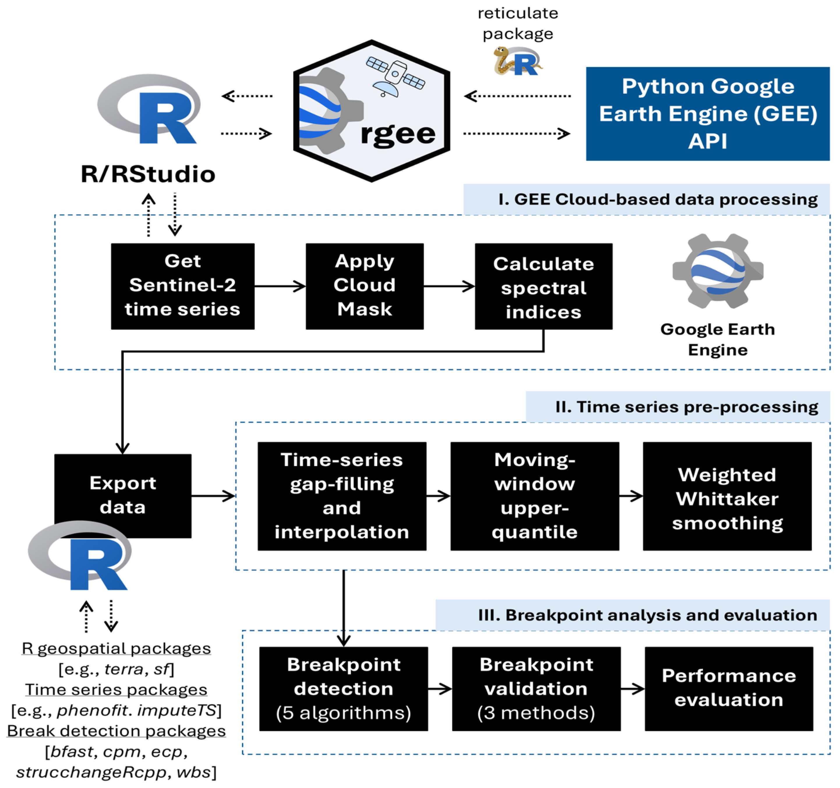
The analysis pipeline comprises several sequential steps for accessing, pre-processing, and analyzing Sentinel-2 time-series data to monitor individual trees (Figure 2). This includes data acquisition via Google Earth Engine, the application of cloud removal masks, and the computation of spectral vegetation indices. The remaining steps were performed in R (version 4.5.2), including time-series gap-filling, regularization and interpolation, smoothing, deseasonalization, and detection of significant negative/downtrend breaks indicative of potential tree loss.

2.2.1. Satellite Data Extraction and Preparation

Sentinel-2 multispectral imagery was used to derive spectral/vegetation indices’ time series for individual large-tree locations. Data was accessed via Google Earth Engine (GEE) using the rgee (v.1.1.8) R package.
We tested four spectral indices (SIs) for tree-level monitoring: EVI2 (Enhanced Vegetation Index 2), NDVI (Normalized Difference Vegetation Index), NDRE (Normalized Difference Red Edge), and NBR (Normalized Burn Ratio). These indices include different regions of the electromagnetic spectrum captured by Sentinel-2: the red portion of the visible spectrum (Red), the near-infrared region (NIR), the red-edge transition zone (Red Edge), and the shortwave infrared region (SWIR). The Normalized Difference Vegetation Index (NDVI), calculated as (NIR − Red)/(NIR + Red) using NIR (band B8, 842 nm) and red (band B4, 665 nm) spectral bands, was employed as a baseline indicator of photosynthetic activity and green biomass density [57], and is a well-established and robust index in the literature, with demonstrated effectiveness for tree monitoring [30]. The Enhanced Vegetation Index 2 (EVI2), a two-band modification in the original EVI expressed as 2.4 × [(NIR − Red)/(NIR + Red + 1)], was selected for its improved sensitivity in high-biomass areas and reduced atmospheric influence [58]. Both NDVI and EVI2 can be computed at Sentinel-2’s native 10 m spatial resolution. In contrast, the Normalized Difference Red Edge (NDRE), computed as (NIR − Red Edge)/(NIR + Red Edge) using the near-infrared (band B8) and red-edge (band B5, 705 nm) bands, and the Normalized Burn Ratio (NBR), calculated as (NIR − SWIR)/(NIR + SWIR) using the near-infrared (band B8) and shortwave infrared (SWIR, band B12, 2190 nm) bands, rely on red-edge and shortwave infrared bands available at 20 m native resolution. These indices were resampled to 10 m resolution in GEE for consistency in tree-level assessments. NDRE was included to capture variations in chlorophyll content and early stress detection, particularly valuable in mixed forest stands [59]. The NBR index was tested for its capacity to detect fire scars, forest disturbances, and moisture stress in woody vegetation [60].
We extracted the SI time series for each tree based on two distinct situations: (i) the tree point coordinates (pixel value where the tree is located), and (ii) the mean value of a 20 m buffer area surrounding each tree point, to test whether spatial context variations in the immediate surroundings could help improve classification results. This buffer size approximates a 3 × 3-pixel neighborhood (diagonal ≈ 21.2 m) at Sentinel-2’s 10 m resolution and aims to compensate for the lack of tree-specific crown-dimension data.
Two Sentinel-2 products were compared to evaluate the trade-off between temporal coverage and atmospheric correction quality: (i) the Level-1C product (L1C-Top-of-Atmosphere reflectance, without atmospheric correction), tagged COPERNICUS/S2_HARMONIZED in GEE, and (ii) the Level-2A product (L2A-Bottom-of-Atmosphere reflectance, with atmospheric correction, tagged COPERNICUS/S2_SR_HARMONIZED). The L1C product was used to extend the time series back to mid-2015, whereas the L2A product is only available from the first quarter of 2017 onwards. Although it had a shorter temporal coverage, the L2A product was expected to improve results due to the atmospheric corrections applied during processing. Cloud masking was applied using the QA60 band to filter out clouds, cloud shadows, and cirrus. The varying temporal resolution (10-day revisit from June 2015 to March 2017, and 5-day thereafter) and reduced valid observations due to cloud cover yielded an irregular SI time series for each location over the study period.

2.2.2. Time-Series Gap-Filling, Interpolation, and Smoothing

After processing, the SI series were regularized to a daily time step to enable consistent analysis. All observation dates were placed on a daily timeline between the series start and end, and missing days were imputed using linear interpolation in the R package imputeTS (v.3.4) [61]. This step was necessary to ensure that the estimated breakpoint dates provide the best possible approximation to the actual day of tree felling (if it exists). It also provides a consistent, regular time series for subsequent steps, which break detection algorithms require. This step produced a continuous daily SI trajectory for each tree while preserving observed values and replacing cloud-induced gaps with plausible estimates.
To mitigate residual cloud noise or short-term fluctuations, a moving-window (MovWin) quantile filter was applied. A 9-day sliding window (±4 days around the focal day) was used, within which the 95% percentile of each SI was computed for each day. This filtering process produces a high-pass envelope of the SI signal, effectively suppressing isolated low outliers (e.g., brief drops from cloud shadows) while retaining the upper level of greenness with lower uncertainty. The result is a moving-window series representing the local upper bound of the SI.
Finally, a Whittaker smoothing filter was applied to the daily series. The Whittaker smoother (Smo) is a penalized least-squares method that balances fidelity to the data with temporal smoothness [62], controlled by a smoothing parameter λ (with larger λ producing a smoother curve [63]). We employed λ ≈ 5000 as a suitable compromise to preserve the SI signal while removing noise. Importantly, we implemented an upper-envelope weighting strategy to avoid bias from spurious low values [64]. Observations with SI above a threshold (the 35% percentile of the series) were given full weight (1.0). In contrast, lower values (likely affected by clouds) were down-weighted (weight 0.01) in the smoothing algorithm. This approach, similar to the modified Whittaker smoother of Atzberger & Eilers [64], ensures that the fitted curve adheres to the upper envelope of the SI, thereby reducing uncertainty. This smoothing filter was also applied to the previous moving-window series (MovSmo) (without additional weighting, since the windowing already removed outliers). The result was a daily, smoothed SI time series per tree, capturing the seasonal vegetation dynamics while filtering high-frequency noise [65,66]. Whittaker smoothing used the “whit2” method from the phenofit (v.0.3.11) R package [67]. Before breakpoint analysis, the SI time series were deseasonalized using Seasonal Trend decomposition using LOESS (STL) from the R stats (v.4.5.2) package, with seasonal adjustment applied via the “seasadj” function from the forecast (v.9.0.2) package [68,69], allowing the break detection algorithm to focus on structural changes in the non-seasonal components.
Hereafter, the pre-processed SI time series are referred to as “datasets” and consist of three variants: (i) moving-window pre-processing only (Mov), (ii) smoothing only (Smo), and (iii) a combination of moving-window followed by smoothing (MovSmo). Each dataset was evaluated independently to assess its effectiveness in detecting breakpoints.

2.2.3. Break Detection Methods

We compared multiple general-purpose breakpoint detection algorithms currently available in R to identify abrupt decreases in the pre-processed SI time series that correspond to potential tree-felling events. To avoid confounding seasonal phenological changes with disturbances, detection was performed on deseasonalized data (obtained by removing the seasonal component via STL decomposition) for most algorithms. When an algorithm detected multiple breaks, we retained the break with the largest negative change, as this is most likely to reflect a tree-felling event. Descriptions of each algorithm are provided below.
Breaks For Additive Season and Trend (BFAST01): A decomposition-based approach that fits a seasonal-trend model to the time series and then tests for structural breaks in the trend and seasonal components [70]. We used a simplified framework in the R bfast package (v.1.7.1) [71], which checks for one single major break in the time series using an OLS-MOSUM test with an unknown break date at the 5% significance level. This method can inherently model seasonal cycles (using harmonic terms) and detect a break as an abrupt shift in the series [72].
Structural change in linear regression (STC): A regression-based multiple breakpoint detection [73] implemented in the strucchangeRcpp (v.1.5-4–1.0.1) package [36,74]. It finds the optimal locations of one or more breaks by minimizing the residual sum of squares in a piecewise linear fit. Here, we constrained the method to detect the largest breakpoint in the SI time series (i.e., indicative of tree loss). A minimum segment size of 15% of the series length was enforced to avoid overfitting. This approach evaluates a null hypothesis of no change against a one-change alternative using the sup.F or MOSUM tests [71].
Energy-divisive (ED): A nonparametric change-point detection using the energy statistic from the ecp (v.3.1.6) package [38]. This divisive algorithm does not assume a particular distribution; it iteratively partitions the series to maximize differences in distribution between segments. We applied it to the SI series to identify significant changes in distribution, with a significance level of 0.05 and a minimum segment length of min_size = 30 days to avoid spurious short-term changes. Parameter k (number of change point locations to estimate) was set to 1 (one single most significant breakpoint), R = 1000 (maximum number of random permutations), and alpha = 1 (as the moment index used for determining the distance between and within segments).
Change point model (CPM): This is a sequential change detection approach using the cpm (v.2.3) package [75] to detect a change in mean SI values. We employed an exponential-weighted moving average change-point model [75] with an average run-length threshold ARL0 ≈ 500 (i.e., a 0.2% false-alarm rate) to detect a shift. The CPM method is a sequential (Phase II) break detection. This means that, in this framework, observations are processed sequentially, and after each observation, a hypothesis test is conducted to assess whether a statistically significant change has occurred. Once the test statistic exceeds a predefined threshold, the procedure terminates and returns the estimated change-point (or break) location without processing subsequent observations.
Wild-binary segmentation (WBS): A multiple breakpoint technique that improves sensitivity to changes of any size by analyzing many random sub-intervals of the series [39]. Using the R wbs (v.1.4.1) package, we generated M = 1000 interval partitions and applied binary segmentation to detect if and where the mean SI values changed within each interval. WBS is statistically consistent and well-suited to detecting abrupt drops, even amid other gradual changes. In our application, we allowed the algorithm to report the largest break found.
As a baseline, these algorithms were also compared against the Continuous Change Detection and Classification (CCDC) approach. CCDC is a well-known method tailored to satellite time series, currently implemented in GEE. CCDC is a model-based time-series segmentation approach for detecting structural changes in multi-temporal satellite data [40]. Unlike the other algorithms, which were applied to deseasonalized SI time series after R pre-processing, CCDC explicitly models seasonality and long-term trends using harmonic regression fitted to multi-band data. Breakpoints are identified as statistically significant deviations from the fitted model. In this study, we applied CCDC to Sentinel-2 time series (2015–2025) using spectral bands and vegetation indices. To focus on disturbances consistent with tree-felling, we retained only breakpoints with high confidence (change probability ≥ 0.99) and negative magnitude in the NIR band. When multiple breakpoints were detected for a given tree, we selected the breakpoint with the largest negative NIR change. The presence or absence of such a breakpoint was then used as a binary indicator of potential tree-felling.
Hereafter, we will refer to each method as an “algorithm”. Each one of the five algorithms was evaluated independently (combined with dataset variants) to assess its effectiveness in detecting breakpoints in the SI time series.

2.2.4. Post-Analysis Validation of Detected Breakpoints

Each break detection algorithm produced either a candidate break date or none. Because not all detected SI breaks correspond to tree-felling events (e.g., breaks can originate from abrupt increases in spectral indices), a post-validation step was fundamental to distinguish actual tree loss from spurious detections. This post-validation is based on the principle that tree felling must always produce an immediate and/or abrupt reduction in SI values, regardless of subsequent recovery, allowing breaks driven by positive or transient signal changes to be identified as false alarms. Three distinct post-analysis validation strategies were implemented:
(i)
Long-term median percent difference—computes the median SI values before and after the detected break using all available observations in each period. The percent difference is calculated as follows: [(SI_post − SI_pre)/SI_pre × 100]. In this case, a break is classified as “valid” when this value is equal to or lower than −10%, indicating a substantial reduction in a given spectral index.
(ii)
Short-term median percent difference—follows the same approach as (i) but restricts the calculation to a 30-day window immediately before and after the detected break. The same −10% threshold is applied to the resulting percent difference to determine whether the break is considered “valid”, thereby emphasizing short-term changes while reducing the influence of longer-term variability/recovery;
(iii)
Short-term randomized trend—evaluates whether the detected break is associated with a statistically meaningful negative change in the SI values by comparing the local post-breakpoint trend against pre-break behavior. A centered temporal window is defined around the detected break, and a robust Theil–Sen slope (using package robslopes (v.1.1.4); [76,77]) is estimated and expressed as a percent change per year relative to the pre-break median SI values. To account for natural variability and partial recovery, a null distribution of slopes is generated by repeatedly sampling equally long, contiguous windows from the pre-break period and computing their corresponding slopes. A break is considered “valid” if the post-breakpoint trend is either sufficiently negative (slope ≤ −10%/year), significantly more negative than the pre-break null distribution (one-sided p ≤ 0.1), or if post-breakpoint SI values remain persistently depressed relative to the pre-break baseline.
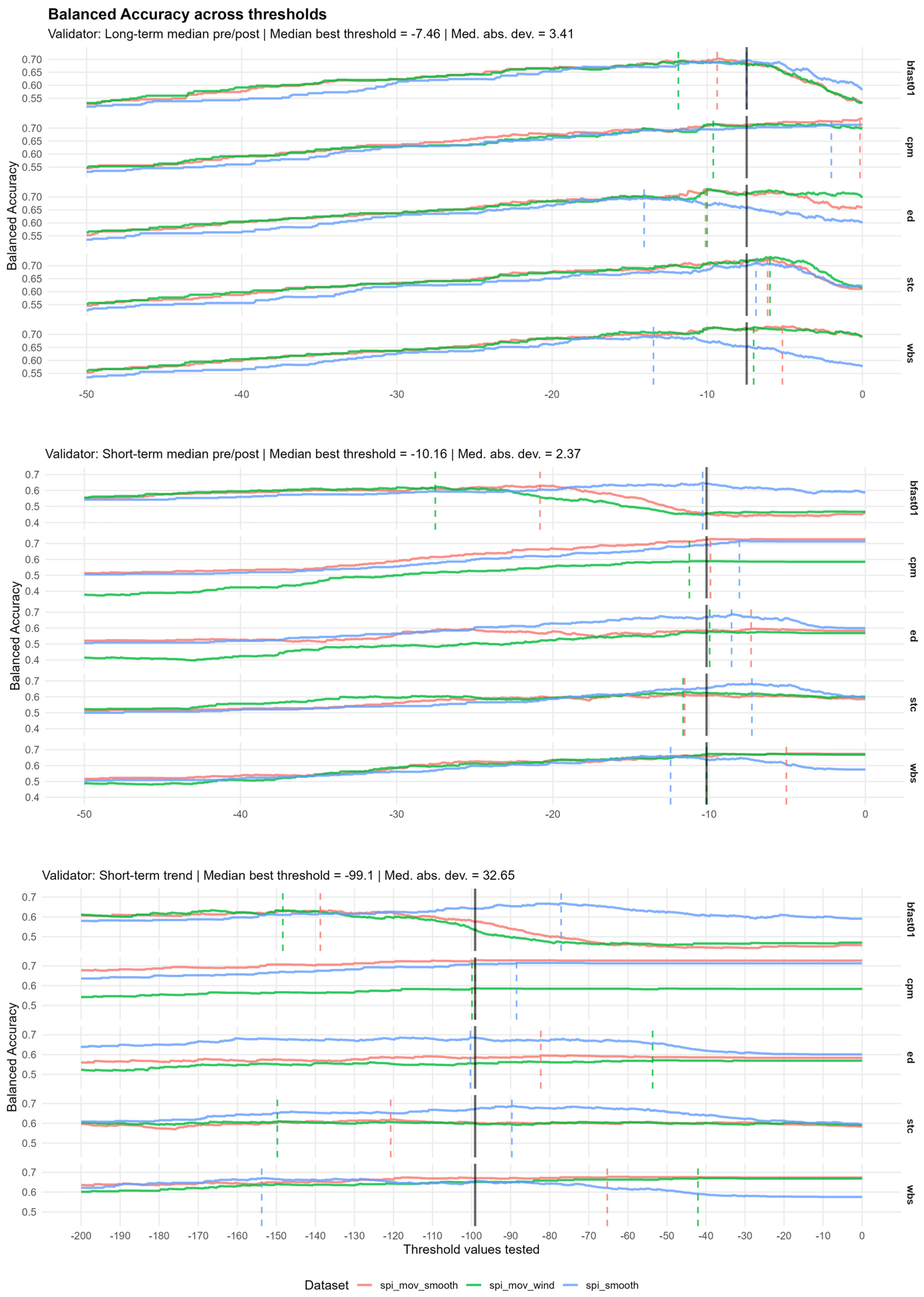
Hereafter, we will refer to each validation method as a “validator”. Each validator was also evaluated independently (combined with algorithm and dataset variants) to assess its effectiveness in detecting breakpoints in the SI time series. To complement this evaluation, we conducted a sensitivity analysis to identify the optimal threshold for each post-validation method based on the best-performing SI. Balanced accuracy was recalculated for each algorithm/dataset combination across a predefined range of threshold values. For the long- and short-term median validators, thresholds ranged from −50% to −0.001% in 0.05% increments, whereas for the trend-based validator, thresholds ranged from −200% to −0.001% in 0.2% increments [see Appendix C.1 for further details].

2.2.5. Evaluation of Break Detection Performance

Break detection performance was evaluated using ground-truth data from field surveys, which indicated the status of each monitored tree (dead/felled vs. alive/not-felled). For each combination of break detection algorithm, input dataset, and validation strategy, the detected break events were compared against the corresponding ground-truth observations. A detected break was classified as a true positive (TP) if the algorithm identified a breakpoint in a tree confirmed as felled in the field, and as a false positive (FP) if a break was detected in a tree that remained unfelled. Conversely, a false negative (FN) occurred when the algorithm failed to detect a break in a confirmed felled tree, and a true negative (TN) when no break was detected in an unfelled tree.
Performance assessment was conducted by constructing confusion matrices, from which the following metrics were derived: balanced accuracy (BA), F1-score (F1), sensitivity (true-positive rate, or recall), specificity (true-negative rate), and precision (positive predictive value). All metrics range from 0 to 1, with higher values indicating better agreement between detected break events and field observations. Sensitivity quantifies the proportion of actual tree-felling events correctly identified by the algorithm (TP/[TP + FN]), reflecting the method’s ability to detect disturbances. Specificity measures the proportion of unfelled trees correctly identified as such (TN/[TN + FP]), indicating the algorithm’s capacity to avoid false alarms. Precision represents the proportion of detected breaks that correspond to actual felling events (TP/[TP + FP]), summarizing the reliability of positive detections. Balanced accuracy was computed as the mean of sensitivity and specificity, thereby providing a performance measure that is robust to class imbalance (i.e., unequal numbers of felled and unfelled trees in the dataset). The F1-score represents the harmonic mean of precision and sensitivity (2 × [Precision × Sensitivity]/[Precision + Sensitivity]). It provides a single metric that balances the trade-off between detecting all felling events and minimizing false detections. Because the evaluated breakpoint detection algorithms are non-learning methods, no model training step was required. Consequently, all available field observations could be used for performance evaluation, and no cross-validation or train/test partitioning was necessary.
Evaluation metrics were computed to allow for comparison of performance across the following tests:
(1)
L1C (Top-of-atmosphere; 2015–2025) product vs. L2A (Surface Reflectance; 2017–2025) product;
(2)
Spectral indices (four in total: EVI2, NBR, NDRE and NDVI);
(3)
Across all combinations of algorithm–dataset–validator;
(4)
Between point-based time series and time series aggregated within a 20 m buffer;
(5)
The entire set of trees (n = 691) vs. a subset of trees for which EVI2 breaks were detected after 2020 (n = 643; for now on named “post-2020” series) to assess the potential influence of Sentinel-2 data accumulation on break detection performance;
(6)
For each tree trait category (i.e., height and DBH classes, genus, botanical class, leaf type, and spatial context), we subsequently averaged across all algorithm–dataset–validator combinations to assess their effect on break detection performance.
All analyses and performance metrics were computed in the R statistical computing environment.

2.2.6. Analyzing the Effect of Analysis Options on Break Detection Performance

To quantify the relative contribution of individual break detection pipeline components to classification performance, balanced accuracy was modeled using a linear model with the algorithm, dataset, and validator specified as fixed categorical effects. Factor effects were evaluated using a Type II analysis of variance (ANOVA), which assesses each main effect after accounting for the presence of the others without assuming a hierarchical ordering. For each factor, degrees of freedom, sum of squares, F-statistics, and associated p-values were computed. Effect sizes were quantified using partial eta-squared (η2), representing the proportion of variance in balanced accuracy attributable to each factor after controlling for the remaining factors.

2.2.7. Analyzing the Effects of Tree Characteristics on Break Detection Performance

To quantify the relative importance of tree characteristics on algorithm performance, we applied a random-effects variance decomposition with balanced accuracy as the response variable. Each tree trait (genus, DBH class, height class, spatial context class, botanical class, and leaf type) was modeled separately as a random effect in a linear mixed-effect framework. For each factor, the between-level variance was extracted and adjusted for the number of levels to ensure comparability among factors with differing cardinality. This approach allows for the identification of the tree characteristics that most strongly contribute to variability in algorithm performance while avoiding biases associated with unequal group sizes or factor complexity.

3. Results

3.1. Composition and Structural Variability of the Selected Tree Sample

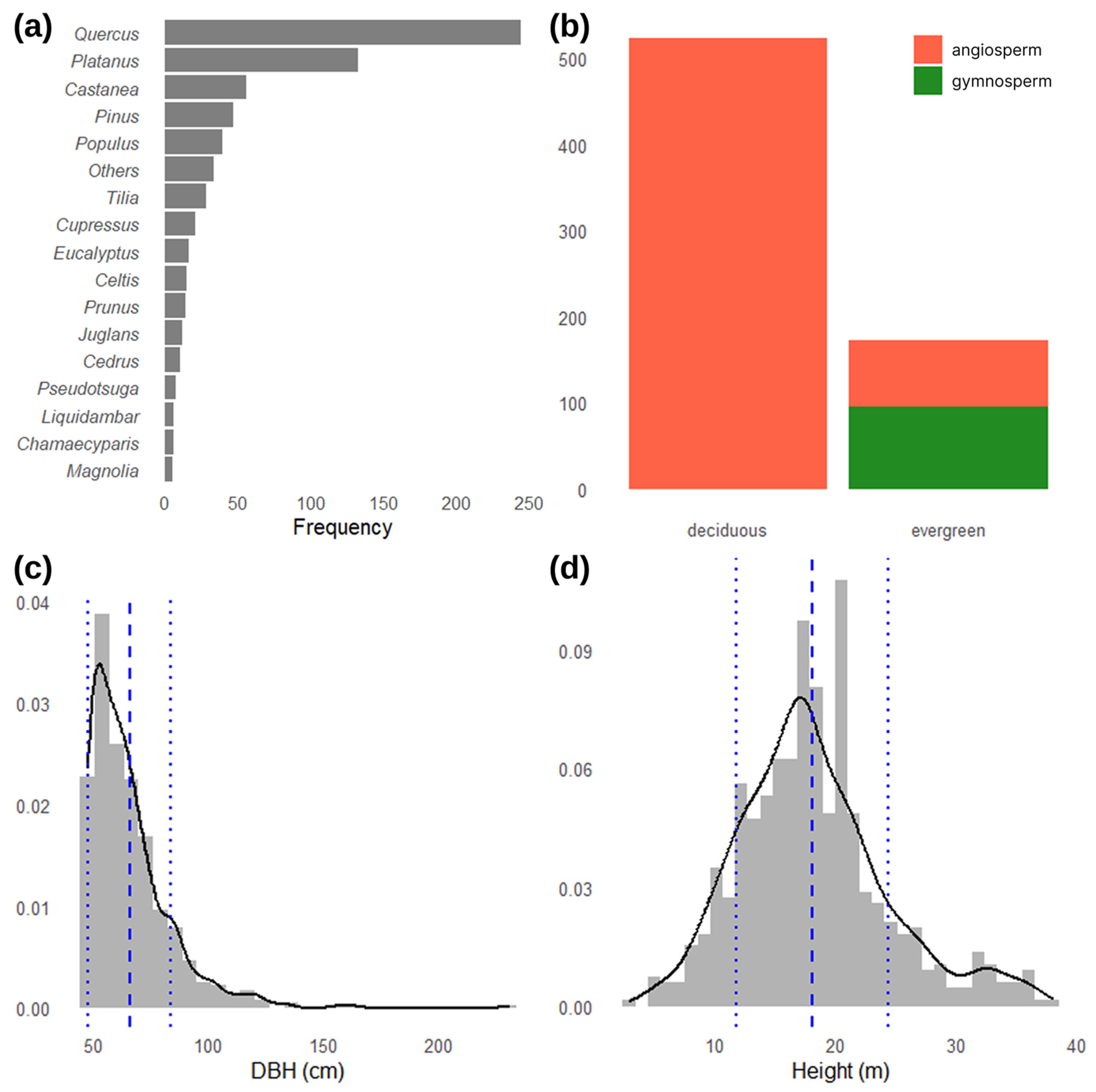
The selected tree sample used for break detection analysis and performance evaluation comprises individuals from a diverse range of species and structural attributes (Figure 3; Appendix A.1 for further details). The most-represented genus is Quercus, followed by Platanus and Castanea, while a long tail of less-frequent genera is grouped under “Others” (Figure 3a). In botanical classification, the majority of trees are deciduous angiosperms, with evergreen gymnosperms comprising a smaller proportion (Figure 3b).
The structural profile of the trees, as measured by diameter at breast height (DBH) and total height, follows distinct patterns. DBH exhibits a right-skewed distribution, with most trees having relatively small diameters; the mean DBH is approximately 63 cm (±24 cm), though values range up to over 200 cm (Figure 3c). In contrast, tree height follows a near-normal distribution, with a mean height of approximately 19.5 m (±6.4 m) (Figure 3d). Regarding tree status, approximately 20.5% are classified as felled, with variation across grouping factors. These distributions encompass a wide range of tree sizes, conditions, and ages, from smaller or younger individuals to older, mature trees, thereby contributing to the dataset’s heterogeneity and representativeness (see Appendix A.1 for further details).

3.2. Time-Series Visual Assessment

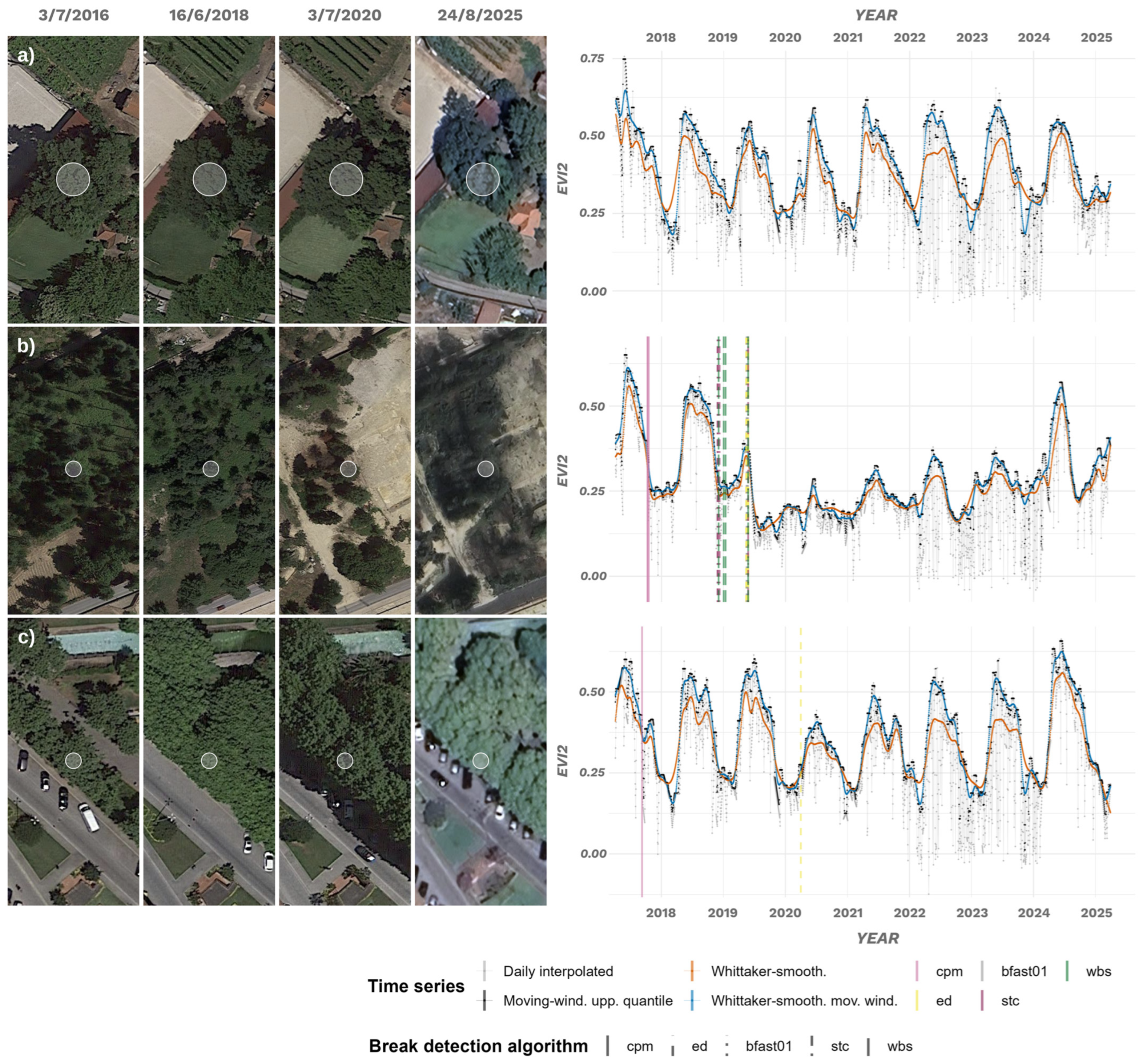
Integrating visual assessment of SI time series with field observations provided critical insights into tree status at the landscape scale (Figure 4). The assessment revealed a high degree of heterogeneity in conditions, often extending beyond what can be reliably observed through local field-based evaluations alone. This diversity of situations includes very stable trees, often characterized by slow, monotonic increases in biomass (Figure 4a). It also encompasses clear-felling events associated with land-use change and construction activities (Figure 4b), which are characterized by abrupt breaks detected by all algorithms and are followed by a relatively slow recovery of surrounding vegetation or canopy closure. In these cases, the seasonal signal/pattern was fundamentally altered and no longer evident after the break.
Visual assessment of SI temporal profiles also revealed a false detection (Figure 4c), characterized by an abrupt break that exceeded the validator threshold. At the same time, the seasonal pattern was preserved, followed by a slow recovery indicative of biomass gain and canopy regrowth. Field observations and inspection of high-resolution imagery confirmed that this case did not correspond to a felling event, but rather to an episode of intensive pruning of an urban tree. Although this disturbance produced a break signal similar to that of tree removal, the persistence of the seasonal SI pattern and continued vegetation recovery indicated that the tree remained alive.
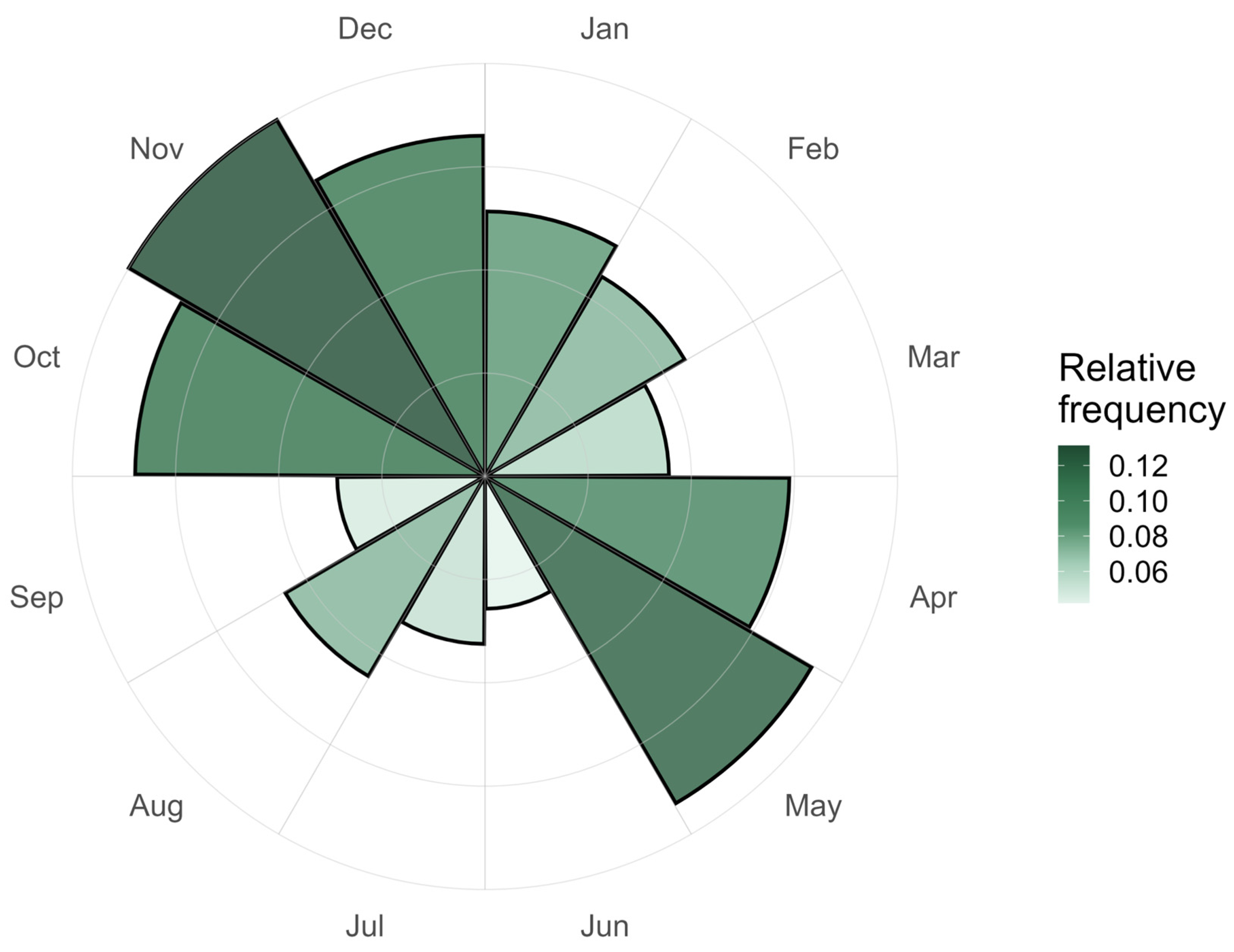
In addition, by understanding which periods of the year are associated with more frequent breaks, it is possible to identify a clear seasonal signal in break detection. In the field validation dataset, satellite-derived break dates (for felled trees) indicate that the felling of large trees was unevenly distributed across the year, with the highest frequencies occurring in autumn and winter seasons, namely November (13.1%), October (11.1%), and December (10.8%) and later in the spring season for April (9.7%) and May (12.0%). Compared with the mid-year period (June–September), lower frequencies were observed, accounting for ~21.6% of the combined observed events during this period (Figure 5; see Appendix A.2 for further details). This indicates that most trees are identified as felled or dead during the autumn–early winter and spring periods. At the same time, summer months show considerably lower frequencies, resulting in a distinctly non-uniform temporal distribution of break events.

3.3. Evaluation by Algorithm, Pre-Processing Dataset and Validator

To identify the analysis components with the highest average performance, namely the break detection algorithm, pre-processing dataset, and post-validator, we evaluated the mean performance of each component independently. The following subsections present these results.

3.3.1. Comparison of Break Detection Algorithms

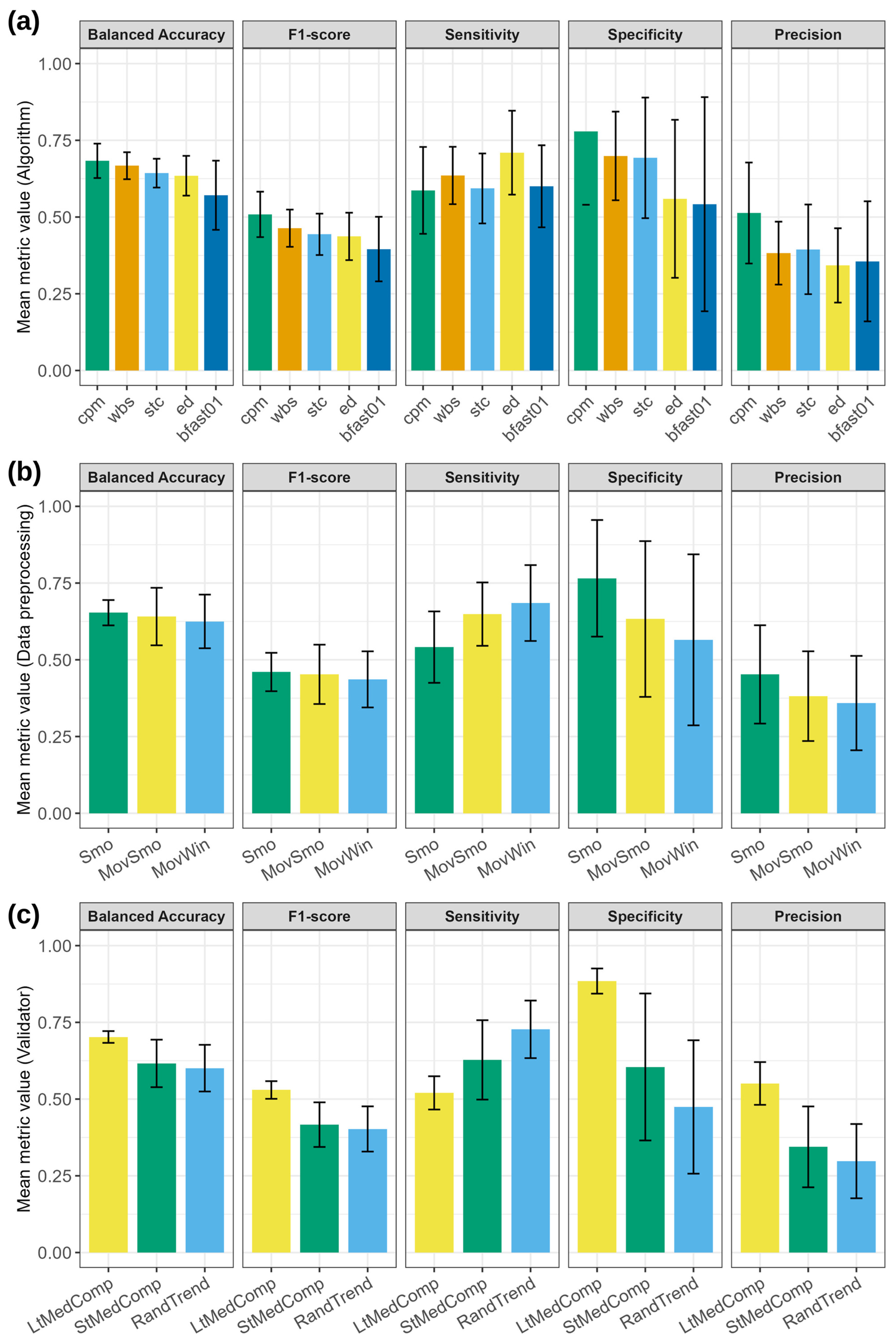
Among the evaluated break detection algorithms, and as seen in Figure 6a (see Appendix B.1 for further details), the change point model (CPM) achieved the best average performance, obtaining the highest BA (0.68 ± 0.06) and F1-score (0.51 ± 0.07), as well as the highest specificity (0.78 ± 0.24) and precision (0.51 ± 0.16). These results indicate that, on average, CPM is the most effective method for detecting true break events. However, its advantage over the wild-binary segmentation (WBS) is small, with more significant differences in sensitivity, specificity and precision, while having a variance in balanced accuracy of only ~0.01, which is well within the variability in the estimates. Overall, these two algorithms constitute the first tier of performers. CPM exhibited superior specificity (0.78 ± 0.24) and had the worst sensitivity of all algorithms (0.59 ± 0.14), suggesting fewer false positives.
Preliminary results for the “baseline” Continuous Change Detection and Classification (CCDC) approach showed consistently lower performance than that of general-purpose breakpoint detection algorithms. In particular, CCDC achieved a balanced accuracy of approximately 0.61 and an F1-score of around 0.39, both substantially lower than those of the best-performing methods (see Section 3.4.1). This was mainly driven by its lower sensitivity (≈0.42), indicating a limited ability to detect true tree-felling events, despite maintaining relatively high specificity (≈0.81). Consequently, considering its performance and the lack of R implementation, CCDC was excluded from further comparative analysis.

3.3.2. Comparison of Data Pre-Processing Approaches

Data pre-processing played a role in shaping detection outcomes, as shown in Figure 6b (see Appendix B.2 for further details). Among the three tested pre-processing pipelines, the smoothing-only (Smo) dataset consistently yielded the best average performance, achieving the highest balanced accuracy (0.65 ± 0.04), F1-score (0.46 ± 0.09), sensitivity (0.68 ± 0.12) and precision (0.45 ± 0.16). This approach appears to mitigate seasonal and cloud-related noise while maintaining higher sensitivity compared to 0.62 ± 0.16; maximum 0.64 ± 0.16 for MovWin and specificity (0.67 ± 0.19; maximum 0.70 ± 0.19 for Smo. In contrast, the moving-window-only (MovWin) showed lower average performance on BA, F1-score, sensitivity and precision, with the highest specificity of all (0.77 ± 0.19). The combined moving-average and Whittaker smoothing (MovSmo) dataset achieved intermediate results across all metrics. These findings indicate that, on average, Smo provides the most effective pre-processing strategy for enhancing break detection in Sentinel-2 EVI time series, offering the best trade-off between noise reduction and signal preservation.

3.3.3. Comparison of Post-Validation Strategies

The post-validation criteria also influenced model performance, as shown in Figure 6c (see Appendix B.3 for further details). The highest average accuracy was achieved by the long-term median approach (LtMedComp), with the best balanced accuracy (0.70 ± 0.02), F1-score (0.53 ± 0.03), specificity (0.88 ± 0.04) and precision (0.55 ± 0.07). However, this validator exhibited the worst sensitivity (0.52 ± 0.05), reflecting a conservative behavior that reduces false positives at the cost of more missed detections. The short-term median approach (StMedComp) performed moderately across all metrics. In contrast, the trend-based validator (RandTrend) yielded the lowest values across almost all metrics, but the highest Sensitivity (0.73 ± 0.09), indicating a tendency to yield more false positives while maintaining lower specificity (0.47 ± 0.22).
A sensitivity analysis was conducted to assess and optimize the threshold values for the post-validation methods [see Appendix C.1 for further details]. The results point out that the used values are already within the interval of the best median values (Median ± MAD) for the long-term (−7.46 ± 3.41%) and short-term median validators (−10.16 ± 2.37%). However, we found that the threshold for the short-term trend validator was outside the intervals from the sensitivity analysis, which should be closer to −99.10 ± 32.65% compared to the −10% used. The results from the sensitivity analysis also suggest variation in threshold values across break detection algorithms and datasets. This means that some degree of fine-tuning should be considered to adjust thresholds, especially because some combinations may require more conservative values (e.g., long-term median ED/Smo: −14.06%, WBS/Smo: −13.46% or BFAST01/MovWin: −11.86%) compared to others that are more permissive (e.g., long-term median CPM/MovSmo: −0.15%, CPM/Smo: −2.00% or WBS/MovSmo: −5.16%). Contrary to our expectations, the sensitivity analysis yielded only a marginal improvement in maximum balanced accuracy, from 0.73 for ED/MovSmo using the selected threshold to 0.74 for CPM/MovSmo using the optimal long-term median threshold. Overall, this suggests that the selected threshold values were already very close to optimal.

3.4. Comparative Evaluation of Break Detection Performance

3.4.1. Best Performing Combinations

Break detection performance was highest when combining the EVI2 or NDVI (L2A) vegetation index, the energy-divisive algorithm (ED) with the moving window or the combined smoothing + windowing dataset and the long-term median validator, achieving a balanced accuracy (BA) of 0.73 (F1 = 0.55–0.56, sensitivity = 0.60–0.61, specificity = 0.85–0.86, precision = 0.50–0.53). Very similar performance was obtained using the change point model (CPM) with the combined smoothing + windowing dataset and the short-term median or trend validator, yielding BA of 0.73 (F1 = 0.55, sensitivity = 0.61–0.63, specificity = 0.83–0.84, precision = 0.48–0.50). Also, when using the wild-binary segmentation (WBS) algorithm combined with the moving-window dataset and the long-term median validator, similar results can be achieved, with higher specificity and precision (BA = 0.73, F1 = 0.56, sensitivity = 0.56, specificity = 0.89, precision = 0.56). Overall, these combinations are recommended for detecting felling events in large trees, as they provide a balanced trade-off between overall accuracy and sensitivity–specificity.
Other algorithmic combinations also for EVI2 or NDVI (L2A), however, achieved higher sensitivity, which is particularly relevant given that the cost of false detections is relatively lower than that of missed events. Notably, this was observed again for the ED algorithm with moving window or combined smoothing + windowing datasets, both with the short-term trend validator (BA = 0.57–0.58, F1 = 0.37–0.38, sensitivity = 0.86–0.85, specificity = 0.28–0.32, precision = 0.24) and for the same algorithm with the moving window dataset and short-term median validator (BA = 0.58, F1 = 0.37, sensitivity = 0.82, specificity = 0.33, precision = 0.24).
Among the spectral indices, EVI2 and NDVI performed best, both reaching a maximum BA of 0.73 (0.64 ± 0.07), followed by NDRE at 0.70 (0.62 ± 0.05) and NBR at 0.68 (0.59 ± 0.03). Further details are provided in Supplementary Information S2.

3.4.2. Effects of Surrounding Vegetation: Point-Based vs. Buffer-Based Time Series

To assess the effects of surrounding vegetation, we compared break detection results from point-based time series (single-pixel values) with those from buffer-based time series (mean SI within a 20 m radius). The best-performing results achieved a BA of 0.70 (F1 = 0.51–0.53, sensitivity = 0.50–0.53, specificity = 0.86–0.90, precision = 0.50–0.56). If higher sensitivity is prioritized, the best result reached 0.81, but with lower overall performance (balanced accuracy = 0.61, F1 = 0.39, specificity = 0.41, precision = 0.26). Overall, the use of a 20 m buffer around tree locations reduced the main performance metrics relative to point-based data, indicating no advantage over the point-based approach (see Supplementary Information S2 for further details).

3.4.3. Effects of Break Detection Series Duration

When considering the full validation set, tests show slightly better performance for the L2A/surface reflectance (SR) time series (2017–2025), which achieved a maximum balanced accuracy (BA) of 0.73 (mean ± SD = 0.62 ± 0.07), compared with 0.71 (0.63 ± 0.06) for the L1C/top-of-atmosphere (TOA) time series (2015–2025). In contrast, we found an overall increase in detection performance when considering the subset of trees whose breakpoint is in 2020 or later. For this subset, L1C/TOA data yielded slightly better results, achieving a maximum BA of 0.78 (0.65 ± 0.07), compared with 0.75 (0.64 ± 0.07) for the L2A/SR. Also, for this subset, the same pattern was observed for the data with the 20 m buffer, where higher BA and sensitivity values were estimated across different combinations of SI, algorithms, pre-processing datasets, and validators (see Supplementary Information S2 for further details).

3.4.4. Effect of Analysis Options on Break Detection Performance

Overall, the results from the ANOVA and partial η2 analysis (i.e., the proportion of variance in the response explained by a given factor after accounting for all other factors; see Appendix B.4) indicate that the validator method has the strongest influence on detection performance (η2 = 0.480, p < 0.001), followed by the choice of break detection algorithm (η2 = 0.407, p < 0.001). In contrast, the pre-processing dataset has a negligible and non-significant effect on performance (η2 = 0.059, p > 0.1; n.s.).

3.4.5. Effect of Tree Traits

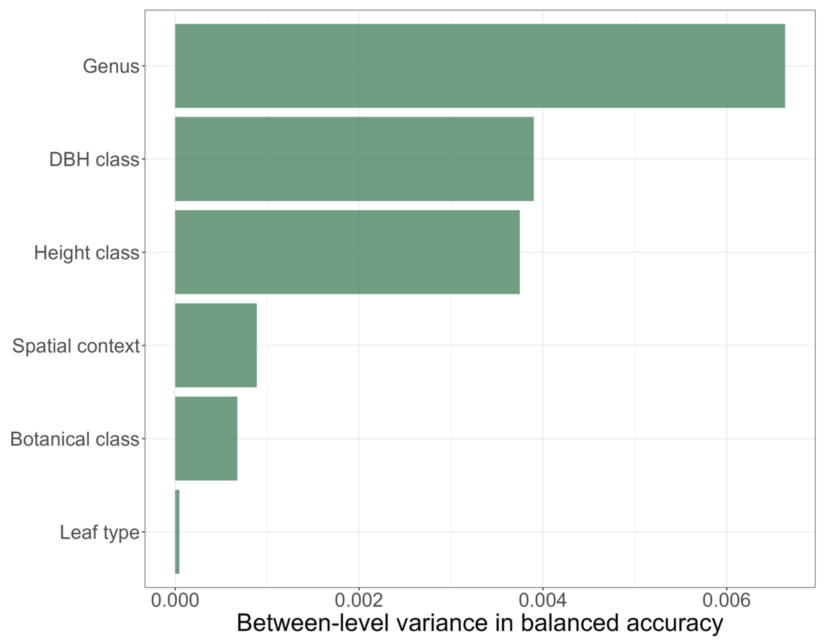
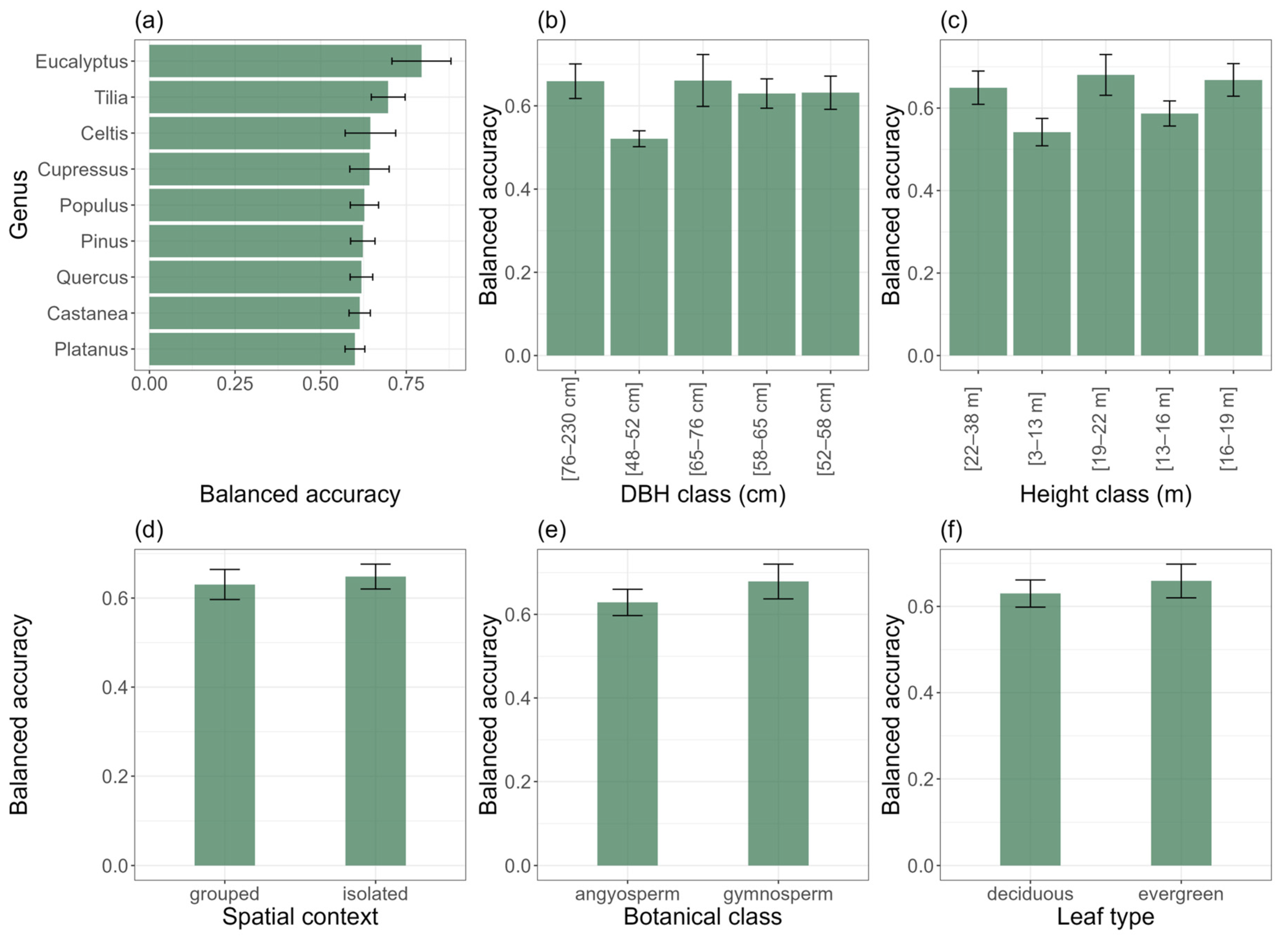
A random-effect variance analysis, adjusted for the number of factor levels, was used to quantify the relative importance of tree traits in explaining variability in balanced accuracy (Figure 7). This analysis identified tree genus and structural traits (DBH and total height) as the dominant contributors to between-level variance. In contrast, spatial context, botanical class, and leaf type explained only a small proportion of the total variance. Guided by these results, balanced accuracy was analyzed across individual trait categories/levels to interpret the observed variance patterns (Figure 8; see also Appendix B.5 for additional details). Performance varied substantially among genera, ranging from 0.79 ± 0.17 for Eucalyptus to 0.60 ± 0.06 for Platanus. The tree structure showed a consistent positive effect. Balanced accuracy increased from 0.52 ± 0.04 in the smallest DBH class to 0.66 ± 0.08 in the largest class, and from 0.54 ± 0.07 for trees shorter than 13 m in total height to 0.65 ± 0.08 for trees taller than 22 m. Traits with low variance contributions exhibited only minor differences: gymnosperms slightly outperformed angiosperms (0.68 ± 0.08 vs. 0.63 ± 0.06), isolated trees marginally outperformed grouped trees (0.65 ± 0.06 vs. 0.63 ± 0.07), and evergreen and deciduous trees showed nearly identical performance (0.66 ± 0.08 vs. 0.63 ± 0.06).

4. Discussion

This study demonstrates the feasibility of using Sentinel-2 spectral indices’ time series, combined with breakpoint detection algorithms, to monitor felling events of individual large trees in fragmented and human-modified landscapes. It builds on previous research (e.g., [25,26,27,78,79]) by extending the use of optical Sentinel-2 time series for fine-grained monitoring of previously mapped large trees, an area that remains underexplored and lacks robust approaches [43,44,45,46,47,48]. This study systematically compares multiple breakpoint detection algorithms available in R, pre-processing strategies/datasets, and alternative post-validation approaches applied to several spectral indices. This evaluation is conducted using a representative set of trees from a highly human-modified landscape and explicitly examines how tree-specific traits influence detection performance.

4.1. Performance of Satellite-Based Detection of Tree Felling Events

Overall, classification performance was moderate but consistent, with maximum balanced accuracy of approximately 73% (all series)–78% (post-2020) under conservative validation, indicating that satellite-based approaches can reliably support tree-level monitoring when data quality issues/constraints are explicitly addressed (e.g., gap filling, time-series smoothing). It should be noted that, in some cases involving intensive tree pruning or canopy loss, tree-felling detection performance would likely improve if these observations were excluded from the evaluation dataset. However, to preserve realism and reflect the full spectrum of conditions encountered in operational monitoring, we deliberately retained these cases. Doing so enables a more comprehensive and nuanced discussion of satellite-based tree assessment in complex, imperfect real-world scenarios.
By comparing the different spectral indices, it was easy to identify those that would better suit this analysis. EVI2 and NDVI performed best, yielding similar results across all assessed metrics, with a slightly higher balanced accuracy value for EVI2.
Among the evaluated methods, the choice of algorithm emerged as a significant determinant of performance. The change point model (CPM) [75] achieved the best overall results across most assessed metrics (balanced accuracy, F1-score, specificity, and precision), but had the worst sensitivity among all algorithms. For this metric, the energy-divisive (ED) algorithm [38] achieved the highest values. This highlights the trade-off between permissive and conservative detection strategies. Differences among pre-processing methods/data were comparatively small, confirming that while smoothing and interpolation improve signal stability, they cannot compensate for fundamental differences in detection logic.
We also evaluated a remote sensing-specific approach (CCDC) commonly used for large-scale forest disturbance monitoring. However, its performance was lower than that of the best general-purpose breakpoint detection algorithms, particularly due to limited sensitivity in detecting tree-level disturbances. This likely reflects the fact that CCDC is designed for continuous pixel-based monitoring [40] and may be less suited to capturing subtle or highly localized changes associated with individual tree removal, especially in heterogeneous environments. In addition, its implementation in Google Earth Engine outside the R workflow further limits direct comparability. Together, these factors support the use of general-purpose break detection algorithms implemented in R as more suitable for tree-level applications like this study.
We observed minor differences in break detection performance between Sentinel-2 processing levels, i.e., L1C/TOA vs. L2A/SR, and contrasting results between the full and post-2020 validation sets. This suggests that the image-processing level may not be a major determinant of breakpoint detection performance when tree-felling events produce sufficiently strong declines in spectral indices to be consistently detected. However, this interpretation is constrained by the fact that the processing level is partly confounded with time-series length and data quality, as the L1C/TOA series is longer. In contrast, the L2A/SR series is shorter but based on more highly processed data.
Analysis of variance (ANOVA) confirmed that validator choice explained the largest proportion of performance variance (η2 = 0.480, p < 0.001), followed by algorithm selection (η2 = 0.407, p < 0.001), while the pre-processing dataset had a negligible effect (η2 = 0.059, n.s.). This reinforces that post-validation strategy is the most critical methodological decision, while smoothing or gap-filling primarily improves signal stability without fundamentally altering detection logic.
Given its dominant influence, we examine the impact of the post-validation strategy on detection performance in greater detail. This component represents a critical, and to some extent original, aspect of our workflow that contributes to more accurate detection of tree-felling events. The long-term median approach emerged as the most accurate and stable validation strategy, yielding the most conservative results, maximizing specificity (i.e., true negative rate) at the expense of sensitivity (i.e., true positive rate). In contrast, trend-based validation favored the opposite, prioritizing maximum detection capability (by maximizing sensitivity and detection completeness) and representing a more permissive but less conservative approach to break validation. Sensitivity analysis (Appendix C.1) confirmed that validator thresholds are near-optimal for median-based approaches but revealed that algorithm-specific tuning could further improve performance. Overall, these findings emphasize that the post-validation strategy should align with monitoring objectives, particularly in early-warning or enforcement-oriented applications.
Detection performance improved when restricting the analysis to breaks occurring after 2020, compared to the full 2017–2025 time series. The best configuration achieved BA = 0.78 and when optimized for sensitivity, performance reached 0.88 (BA = 0.58–0.60). This improvement likely reflects two complementary factors: longer pre-break baseline periods enable more robust characterization of stable vegetation conditions and seasonal patterns, while the increased temporal resolution following Sentinel-2B’s launch in 2017 provides denser cloud-free observations. As the Sentinel-2 archive continues to expand, these results suggest that monitoring performance will improve further, facilitating earlier detection of tree-level disturbances and supporting more effective operational responses to forest management challenges.
The 20 m buffer approach, designed to capture surrounding vegetation context, consistently underperformed relative to single-pixel extraction across all performance metrics. This counterintuitive result highlights an important operational consideration: while spatial aggregation may improve signal-to-noise ratios in landscape-scale analyses, it appears to introduce spectral contamination at the individual-tree level, where the disturbance signal is inherently localized. In heterogeneous humanized landscapes, where canopy structure, understory composition, and land cover vary at fine spatial scales, single-pixel extraction provides a more precise representation of tree-specific disturbance events. These findings suggest that, for operational tree-level monitoring systems, simpler point-based/single-pixel approaches may be preferable to spatially aggregated metrics.
It is important to emphasize that the framework is primarily tuned to detect abrupt negative shifts in vegetation indices, consistent with sudden canopy loss. It may not fully capture progressive decline trajectories occurring over multiple seasons (e.g., drought stress, pathogen impacts) or distinguish among disturbance types (felling vs. pruning vs. storm damage) without additional validation.

4.2. Effect of Tree Traits in Satellite-Based Break Detection

An additional contribution of this work lies in the explicit importance of tree-level structural and taxonomic traits for determining the success of break detectability and, consequently, how fieldwork tree-monitoring efforts may benefit from such results.
The random-effect variance analysis showed that tree genus and structural attributes (DBH and height) were consistently associated with variability in detection performance. In contrast, leaf type, taxonomic class, and spatial context contributed comparatively little. Larger and taller trees exhibited higher detectability, likely reflecting reduced spectral mixing at Sentinel-2 resolution (10 m), although tree size may also converge with unmeasured factors such as age or management history. The observed association between higher detection rates and larger tree diameter at breast height (DBH) and height is consistent with findings from previous studies on tree cover assessment [e.g., [80,81,82]], as larger trees typically exhibit stronger and more spatially coherent spectral signals, making disturbance-related changes more readily detectable in satellite time series. The variation observed between genera is not linked to any other particular botanical tree attribute (botanical class or leaf type), reflecting that the results can be particular for each genus or species [28]. Together, these results indicate that tree structure and species identity are key contextual factors influencing EO-based detection of tree loss and should be considered when interpreting algorithm outputs or designing operational monitoring systems. For instance, smaller trees of particular species may require greater effort to validate/monitor changes in their status over time.

4.3. Monitoring Ever-Changing Landscapes

Because field surveys typically rely on single or infrequent visits, they are prone to missing sporadic or recent disturbance events. This limitation underscores the advantages of satellite-based time series, which provide continuous spatial and temporal coverage and enable assessment of disturbances while accounting for seasonal patterns, e.g., [37,70].
The concentration of detected breaks in autumn–winter (November–January: ~35%) and spring (April–May: ~22%; Figure 5) is likely driven by both disturbance timing and seasonal differences in detectability. Reduced canopy activity during the dormant season enhances the sensitivity of optical time series to structural changes, while increased phenological variability in spring and summer may obscure abrupt signals [30,83]. In the study region, winter is typically the period during which most tree management activities occur in urban areas. The dormancy period of deciduous species is usually associated with reduced stress from pruning or other management operations. Furthermore, reduced canopy weight in winter is beneficial for removal operations in cities or clear-cutting in managed forests, as it reduces the effort required for removal and transportation of woody material. Spring (April–May) is also the most beneficial time for tree cutting for firewood, as the removed wood can dry out during the subsequent warm months and be ready for use in the next cold season.
Field observations, combined with a thorough interpretation of SI time series, highlight both the potential and inherent complexity of satellite-based tree monitoring. In many cases, tree-felling events were clearly reflected by abrupt changes in vegetation indices, demonstrating that EVI2 or NDVI can effectively capture major structural disturbances at the pixel level, e.g., [41,72,83,84]. However, in heterogeneous, dynamically managed landscapes, the signal associated with tree removal is often modulated or obscured by proximal or concurrent vegetation and land-use dynamics. Rapid changes often follow tree loss, including crop expansion, shrub encroachment, pasture development, and, most commonly, conversion to urban uses. Although tree felling most frequently leads to reductions in SI values, it may also be followed by relatively stable or even increasing SI trajectories when surrounding vegetation rapidly compensates for tree loss, contradicting validator logic that assumes SI reductions expressed as median decreases or negative trends. While SI reductions account for the vast majority of cases, justifying the use of validators to reduce false detections, SI time series and validation logic may fail to capture less common situations such as rapid vegetation growth following felling.
Conversely, abrupt declines in vegetation indices were not always associated with tree removal. Severe pruning, storm damage, partial crown loss, changes in surrounding land cover, or the influence of nearby built structures frequently produced spectral–temporal signatures similar to those of felling, despite trees remaining alive (Figure 4c). These situations emphasize that vegetation index breakpoints reflect changes in the integrated vegetation signal within a pixel rather than the status of a single tree. As such, individual-tree assessment becomes increasingly challenging in heterogeneous or rapidly changing landscapes, especially given the 10–20 m spatial resolution of Sentinel-2. Taken together, these findings underscore that satellite time series provide valuable, scalable information for detecting major disturbances affecting large trees, but their interpretation requires careful consideration of local land-use dynamics, vegetation composition, post-disturbance pathways, and management practices [85,86]. Future developments in post-validation logic (e.g., ensemble decision rules, multi-algorithm consensus) coupled with more advanced break detection algorithms are expected to improve the detection of diverse tree-related changes while reducing ambiguity in complex settings.

4.4. Applications of Breakpoint-Based Monitoring for Large-Tree Loss in Humanized Landscapes

This study presents insights into how open-source data can be used to monitor disturbances affecting individual large trees in humanized landscapes. These large trees act as long-term ecological repositories [4,5] and are undergoing continuous threat worldwide [2,11,13,15]. EO-based detection systems, such as the one presented here, can be adapted to monitor large catalogs of trees that have already been mapped by various efforts worldwide, enabling diagnosis of trends in large-scale tree loss at regional, national, or continental scales, which are impossible to achieve on a periodic basis using only field-observation methods. By enhancing the use of these systems, it is possible to quantify the current, past, and future dimensions of the pressures these features face, improve the identification of trees requiring conservation schemes, and ultimately sustain species in their habitats while enhancing ecosystem services.
Despite some limitations, the proposed methods are particularly well-suited to analyzing large volumes of data in inventories of large trees and assessing their medium-term persistence. Although detecting very recent changes over short time scales (e.g., days) remains challenging, especially given the revisit frequency and noise in satellite optical time series, these approaches enable robust retrospective evaluation of tree continuity/retention and survival, e.g., [25,26,84]. Near-real-time detection is further constrained during autumn–winter months, when reduced illumination, increased cloud cover, and phenological variability reduce image quality and availability [87,88], paradoxically coinciding with peak tree-removal activity (Figure 5). Consequently, the proposed framework should be viewed primarily as a reactive monitoring tool, with an expected operational delay of weeks, suitable for evaluating tree maintenance activities, retention programs, and longer-term outcomes, with operational systems potentially requiring intensified ground-based surveillance during seasons when satellite-based detection is least reliable.
By integrating tree-level structural and taxonomic traits with citizen-science mapping into a scalable Earth observation framework, it becomes possible to operationalize monitoring at unprecedented scales. In this context, the “Green Giants” citizen-science project in Portugal exemplifies this potential: trained citizen-scientists mapped over 20,000 large trees at the national level in 12 months [89], recording georeferenced locations, functional traits, and tree-related microhabitats (TreMs). All these trees can now be monitored remotely using the methods presented here, with the results validated by the citizen-science community. Future conservation strategies can thus build not only on spatial distribution data, but also on status and trend information derived from both citizen observations and Earth observation time series, expanding the evidence base supporting active retention strategies. Given that large trees contribute disproportionately to biodiversity and ecosystem functioning [1,2,3] and their loss is irreplaceable within human timescales, particularly under climate change, integrated systems to value and protect them are increasingly critical.
Datasets combining georeferenced large trees with satellite-derived status assessments can inform active tree-retention strategies across contexts. They support the development of environmental and sustainable tourism programs, community engagement strategies, and policy compliance monitoring (e.g., EU Deforestation Regulation, EU Restoration Law). They can also serve as tools for early auditing and monitoring in forest certification schemes (e.g., PEFC [90], FSC [91]), sustainable finance mechanisms [92], and carbon and biodiversity credit markets [93,94], where transparent, remotely-verifiable evidence of tree persistence strengthens credibility.
Particularly in forested landscapes, the proposed framework offers a complementary perspective to existing large-scale monitoring systems for deforestation and disturbance. While traditional EO approaches are optimized for detecting stand-level or clear-cut events [66,72,78,79], break detection methods applied at the individual-tree scale enable identification of selective logging, canopy gaps, or progressive degradation that may not trigger conventional forest change alerts. This is particularly relevant in managed forests, mixed-use areas, or protected stands where selective removal of large trees can have disproportionate ecological impacts. From a forest management perspective, such tools can support evaluation of harvesting practices, compliance with selective logging regulations, and effectiveness of conservation measures targeting old-growth or habitat trees. By enabling consistent monitoring across large areas, EO-based tree-level analysis provides an additional layer of evidence to support sustainable forest management and biodiversity protection.
In urban environments, these approaches offer a scalable means of tracking the persistence of urban trees across entire cities, enabling identification of gradual decline or abrupt removal events that may otherwise go unnoticed. Such tools can support local or regional authorities by providing independent, spatially explicit evidence of tree loss, thereby enhancing transparency and accountability in urban tree governance. In agricultural landscapes, these methods help reveal long-term trends of landscape simplification and support evaluation of agri-environmental policies aimed at conserving scattered trees [95,96]. Such information is critical for assessing compliance with conservation incentives and identifying areas where additional field-based verification or policy intervention may be required.
Across urban, agricultural, and forested landscapes, a key strength of Earth observation-based tree-level monitoring lies in its ability to capture spatially dispersed or gradual dynamics often overlooked by coarse-resolution or event-driven monitoring systems. Rather than replacing field-based conservation actions, Earth observation-based break detection tools enhance tree preservation by enabling systematic monitoring, prioritized enforcement, and evidence-based policy evaluation. While currently best suited for retrospective and medium-term assessment, these tools provide a critical foundation for future early-warning and preventive monitoring systems.

4.5. Limitations and Future Improvements

Despite the overall consistency of the results, several limitations should be acknowledged, along with potential ways to address them.
First, the spatial resolution of Sentinel-2 is well suited to large, isolated tree crowns but remains challenging for small or clustered trees. In such cases, mixed pixels and spectral interference from neighboring vegetation, highly dynamic land use or built surfaces may reduce detection accuracy, particularly in heterogeneous peri-urban environments.
Second, while Sentinel-2 vegetation indices provide robust indicators of vegetation condition, their sensitivity varies by disturbance type. Visible and near-infrared indices (e.g., NDVI, EVI2) excel at detecting abrupt canopy loss but are less sensitive to sublethal stress such as drought [97,98] or pest-induced decline [99,100,101]. Since our framework targets abrupt negative shifts, consistent with breakpoint detection of tree felling events, it may underrepresent gradual degradation or delayed mortality. Red-edge and SWIR indices (including the tested NDRE and NBR) offer complementary stress sensitivity [87,88,101,102,103,104,105], but Sentinel-2’s native 20 m resolution for these bands may reduce tree-level detectability. Future work combining multi-spectral data at native resolutions with higher-resolution platforms (PlanetScope, LiDAR, SAR) or alternative detection strategies (multi-algorithm consensus, Bayesian, or deep learning approaches) could improve sensitivity to diverse disturbance pathways and enable explicit modeling of progressive change trajectories rather than focusing exclusively on abrupt breakpoints [106,107].
Third, the dataset exhibits class imbalance (~20% felled vs. ~80% alive trees), which may inflate specificity while masking lower sensitivity to the minority class. Although balanced accuracy was used to mitigate this effect, future operational systems should consider stratified sampling or cost-sensitive learning. Additionally, validation thresholds were held constant across algorithms and datasets. Sensitivity analysis (Appendix C.1) indicated that algorithm-specific threshold optimization could improve performance, particularly for the trend-based validator.
Finally, the analysis relies on an uneven distribution of trees across genera and size classes, which may influence variance estimates for less-represented categories. Some uncertainty remains for trees with inferred status based on remote imagery rather than field verification. Expanding field validation efforts and balancing sample sizes across species and size classes would support more robust and transferable operational monitoring systems. These limitations should be considered when interpreting results and when transferring the framework to other regions or ecological contexts.
Looking ahead, the in-depth assessment of detected breaks combined with field observations underscores the importance of developing more generalizable models capable of distinguishing among multiple disturbance types, including tree felling, intensive pruning, drought stress, and pathogen impacts. These findings pave the way for integrated open-source tools for assessing large-tree inventories using satellite time series, including the development of a robust, scalable R package built on the Google Earth Engine platform.

5. Conclusions

This study presents a transferable, open-source framework for detecting abrupt canopy loss in large individual trees using Sentinel-2 imagery, spectral indices’ time series, and statistical break detection methods, with potential applicability to other regions. However, regional calibration of thresholds and seasonal parameters will likely be necessary. The results demonstrate that Earth observation data can support tree-level monitoring and large-tree loss detection even in fragmented and human-modified landscapes. Under conservative validation criteria, the framework achieved a maximum Balanced Accuracy of 73% for the full validation set and 78% when restricting analysis to post-2020 breaks, with particularly high specificity (>85%) for correctly identifying surviving trees.
By integrating satellite observations with field-surveyed trees from the “Green Giants” citizen-science project, this work illustrates the potential of decentralized, data-driven biodiversity monitoring. The proposed framework is relevant to applications such as heritage tree conservation, monitoring of protected or high-value trees, and detecting tree-removal events, particularly in contexts where systematic field monitoring is not feasible.
Future developments should explore multi-sensor data fusion, such as SAR or LiDAR or high-resolution platforms such as PlanetScope. Extending the framework towards near-real-time processing and evaluating alternative break detection/modeling approaches (e.g., AI/Deep Learning, Bayesian Models) may further improve sensitivity to different disturbance types. As pressures on large and old trees continue to increase, scalable EO-based approaches, such as the one presented here, can meaningfully contribute to their monitoring and protection.

Supplementary Materials

The following supporting information can be downloaded at: https://www.mdpi.com/article/10.3390/rs18101519/s1, Supplementary Information S1—Full dataset used for the analysis and results for each tree and Supplementary Information S2—Break detection performance for all possible 1440 combinations of spectral indices, cloud processing methods, algorithms, pre-processing datasets, validators, with or without a 20 m buffer and all (2017–2025) or recent (2020–2025) ground-truth/validation datasets.

Author Contributions

Conceptualization: all authors; Methodology: J.F.G. and J.G.S.; Software, J.F.G. and J.G.S.; Validation, J.F.G. and J.G.S.; Formal Analysis, J.F.G. and J.G.S.; Investigation, all authors; Resources, J.F.G. and J.G.S.; Data Curation, J.G.S.; Writing—Original Draft Preparation, all authors; Writing—Review and Editing, all authors; Visualization, J.G.S.; Supervision, J.F.G., K.T.V., L.A.V. and J.M.; Funding Acquisition, J.G.S. and J.F.G. All authors have read and agreed to the published version of the manuscript.

Funding

This research was funded by Fundação para a Ciência e a Tecnologia (FCT) grant number 2020.05501.BD, DOI:10.54499/2020.05501.BD attributed to Soutinho, J.F.G. and through FCT contract CEECIND/02331/2017/CP1423/CT0012, DOI: 10.54499/CEECIND/02331/2017/CP1423/CT0012, attributed to Gonçalves, J.F.

Data Availability Statement

The original contributions presented in this study are included in this article/Supplementary Materials. Further inquiries can be directed to the corresponding authors.

Acknowledgments

The authors are deeply grateful to Município de Lousada (with particular appreciation to Manuel Nunes, Milene Matos, Pedro Sá and Ana Maria Pereira) and VERDE—Associação para a Conservação Integrada da Natureza (particularly to Cláudia Meca, Raquel Miranda, Rafael Ataídes, João Silva, Simão Quintans, Ana Teresa Vieira, Rita Freitas, Marta Gomes, Marc Tomás and all the involved volunteers) for all the support. The authors further appreciate the reviewer team’s suggestions, which led to significant improvements to the manuscript. During the preparation of this manuscript/study, the author(s) used ChatGPT 5.2 for grammar checking, brainstorming, hypothesis validation, and writing code for the analysis and graphics. ScholarGPT 5.4 and Google Scholar were also used for bibliographic support and referencing. The authors have reviewed and edited the output and take full responsibility for the content of this publication.

Conflicts of Interest

The authors declare no conflicts of interest.

Abbreviations

The following abbreviations are used in this manuscript:
AIArtificial intelligence
BABalanced accuracy
BFAST01Breaks for additive season and trend (for one major break in a time series)
CPMChange point model
DBHDiameter of the trunk at breast height
EDEnergy-divisive
EOEarth observation
EUDREuropean Union Restoration Law
EVI2Enhanced Vegetation Index 2
FSCForest Stewardship Council
GEDIGlobal Ecosystem Dynamics Investigation
GEEGoogle Earth Engine
LiDARLight Detection and Ranging
LtMedCompLong-term median comparison post-breakpoint validator
L1CTop-of-atmosphere reflectance processing level
L2ASurface reflectance processing level
MovSmoCombined moving-average and smoothing pre-processing
MovWinMoving-average filter pre-processing
NDRENormalized Difference Red Edge
NBRNormalized Burn Ratio
NDVINormalized Difference Vegetation Index
NDWINormalized Difference Water Index
PEFCProgramme for the Endorsement of Forest Certification
RandTrendRandomized trend post-breakpoint validator
ROCReceiver operating curve
SDStandard deviation
SmoWhittaker smoother pre-processing
STCStructural change in linear regression models
StMedCompShort-term median comparison post-breakpoint validator
SWIRShort-wave infrared
THTotal tree height
TOATop-of-atmosphere
TreMTree-related microhabitats
WBSWild-binary segmentation

Appendix A

Appendix A.1

Table A1. Descriptive tables with absolute and relative (%) frequencies for grouping factors, including overall distributions and cross-tabulations by tree status (0—not felled, 1—felled). Grouping factors are presented in decreasing order of importance, from the most to the least influential. Bold text highlights grouping factors tested as well as the global totals.
Grouping
Factor
Factor LevelsNRelative Frequency (%)No. Trees Not-Felled (0)No. Trees Felled (1)% Not-Felled (0)% Felled (1)
TOTAL 691100.054914279.520.5
GenusQuercus24435.12004482.018.0
Platanus13219.01092382.617.4
Castanea568.1441278.621.4
Pinus476.8371078.721.3
Populus395.6291074.425.6
Tilia284.0171160.739.3
Cupressus213.016576.223.8
Eucalyptus162.312475.025.0
Celtis152.214193.36.7
Other9714.0712273.226.8
DBH class (cm)[48–52 cm]14721.21222583.017.0
[52–58 cm]11616.71001686.213.8
[58–65 cm]12818.41082084.415.6
[65–76 cm]12417.81042083.916.1
[76–230 cm]12417.81101488.711.3
---568.15478.991.1
Height class (m)[3–13 m]14520.91252086.213.8
[13–16 m]11516.5922380.020.0
[16–19 m]14921.41292086.613.4
[19–22 m]10314.8901387.412.6
[22–38 m]12518.01071885.614.4
---588.34476.993.1
Spatial contextGrouped51574.14189781.218.8
Isolated17625.31314574.425.6
Botanical classAngiosperm59485.547112379.320.7
Gymnosperm9613.8771980.219.8
---50.71020.080.0
Leaf typeDeciduous51974.740811178.621.4
Evergreen17124.61403181.918.1
---50.71020.080.0

Appendix A.2

Table A2. Absolute and relative frequency (%) of break dates per month for felled trees (N = 142) across all combinations of algorithms, processing datasets, and validator methods with valid breaks (Nt = 3658). Bolded rows indicate months with a relative frequency greater than or equal to 10%.
MonthAbsolute FrequencyRelative Frequency (%)
Jan3088.4%
Feb2697.4%
Mar2145.9%
Apr3549.7%
May44012.0%
Jun1544.2%
Jul1955.3%
Aug2697.4%
Sep1724.7%
Oct40711.1%
Nov48013.1%
Dec39610.8%
NTotal3658100.0%

Appendix B

Appendix B.1

Table A3. Average break detection performance by algorithm across all nine combinations of pre-processing dataset (Nd = 3, i.e., moving-average only, smoothing only, and combined moving-average and smoothing) times validator method (Nv = 3, i.e., long-term median, short-term median, and trend). Algorithms include: CPM—change point model, ED—energy-divisive, WBS—wild-binary segmentation, STC—structural change in linear model, and BFAST01—breaks for additive season and trend model.
Break Detection AlgorithmPerformance MetricMeanStandard
Deviation
CPMBalanced Accuracy0.680.06
WBS0.670.04
STC0.640.05
ED0.630.06
BFAST010.570.11
CPMF1-score0.510.07
WBS0.460.06
STC0.440.07
ED0.440.08
BFAST010.400.11
EDSensitivity0.710.14
WBS0.640.09
BFAST010.600.13
STC0.590.11
CPM0.590.14
CPMSpecificity0.780.24
WBS0.700.14
STC0.690.20
ED0.560.26
BFAST010.540.35
CPMPrecision0.510.16
STC0.390.15
WBS0.380.10
BFAST010.360.20
ED0.340.12

Appendix B.2

Table A4. Average break detection performance by pre-processing dataset across all 15 combinations of algorithms (i.e., five breakpoint detection algorithms times three post-validation methods). Pre-processing datasets include: MovWin—moving-average only, Smo—smoothing only and MovSmo—combined moving-average and smoothing.
ClassPerformance MetricMeanStandard
Deviation
SmoBalanced Accuracy0.650.04
MovSmo0.640.09
MovWin0.630.09
SmoF1-score0.460.06
MovSmo0.450.10
MovWin0.440.09
SmoSensitivity0.680.12
MovSmo0.650.10
MovWin0.540.12
MovWinSpecificity0.770.19
MovSmo0.630.25
Smo0.570.28
SmoPrecision0.450.16
MovSmo0.380.15
MovWin0.360.15

Appendix B.3

Table A5. Average break detection performance by break validator method across all 15 combinations of break detection algorithms (i.e., five breakpoint detection algorithms times three pre-processing datasets). Break detection methods include: LtMedComp—long-term median, StMedComp—short-term median and RandTrend—randomized trend.
ClassPerformance MetricMeanStandard
Deviation
LtMedCompBalanced Accuracy0.700.02
StMedComp0.620.08
RandTrend0.600.08
LtMedCompF1-score0.530.03
StMedComp0.420.07
RandTrend0.400.07
RandTrendSensitivity0.730.09
StMedComp0.630.13
LtMedComp0.520.05
LtMedCompSpecificity0.880.04
StMedComp0.600.24
RandTrend0.470.22
LtMedCompPrecision0.550.07
StMedComp0.340.13
RandTrend0.300.12

Appendix B.4

Table A6. Effects of the algorithm, dataset, and validator on balanced accuracy. Type-II analysis of variance (ANOVA) results for balanced accuracy obtained from a linear model including algorithm, dataset, and validator as fixed effects. For each factor, degrees of freedom (df), sum of squares, F-statistic, p-value, and partial eta-squared (η2) are reported. Partial η2 quantifies the proportion of variance in balanced accuracy explained by each factor after accounting for the others, with larger values indicating stronger effects. Effects shown in bold are statistically significant (p < 0.05; α = 0.05).
FactorSum of SquaresdfFp-Valueeta2_p
Algorithm0.06746.16<0.0010.406
Dataset0.00621.120.3360.059
Validator0.090216.63<0.0010.480
Residuals0.09736

Appendix B.5

Table A7. Balanced accuracy by factor/levels including botanical class, genus, height class, size class (DBH), spatial configuration, and leaf type. For each level inside a grouping factor, N_total = 45, which equals the number of break detection algorithms (na = 5) times the number of time series pre-processing datasets (nd = 3) times the number of break validators (nv = 3). This happens because balanced accuracy is calculated for all trees within each combination of algorithm, dataset, validator, and factor level, after which the values are averaged. Grouping factors (in bold) are presented in decreasing order of importance, from the most to the least influential.
Grouping FactorFactor LevelsAverageStandard
Deviation
GenusEucalyptus0.790.17
Tilia0.700.10
Celtis0.650.15
Cupressus0.640.11
Populus0.630.08
Pinus0.620.07
Quercus0.620.07
Castanea0.610.06
Platanus0.600.06
DBH class (cm)[48–52 cm]0.520.04
[52–58 cm]0.630.08
[58–65 cm]0.630.07
[65–76 cm]0.660.12
[76–230 cm]0.660.08
Height class (m)[3–13 m]0.540.07
[13–16 m]0.590.06
[16–19 m]0.670.08
[19–22 m]0.680.10
[22–38 m]0.650.08
Spatial isolationIsolated0.650.06
Grouped0.630.07
Botanical classGymnosperm0.680.08
Angiosperm0.630.06
Leaf typeEvergreen0.660.08
Deciduous0.630.06

Appendix C

Appendix C.1

Figure A1. Sensitivity analysis results for threshold optimization of each post-validation method. The analysis was based on the EVI2 spectral index from surface reflectance (L2A) data, which yielded the best overall performance. The plots illustrate the variation in balanced accuracy across the tested thresholds for each combination of algorithm: cpm—change point model, ed—energy-divisive, wbs—wild-binary segmentation, stc—structural change in linear model, bfast01—breaks for additive season and trend model, and pre-processing dataset: spi_mov_wind—moving-average only, spi_smooth—smoothing only, and spi_mov_smooth—combined moving-average and smoothing. The black line identifies the global median across all algorithms and datasets. The dashed-colored lines indicate the maximum balanced accuracy for each pre-processing dataset.
Remotesensing 18 01519 g0a1

Appendix C.2

Table A8. Sensitivity analysis results for threshold optimization of each post-validation method. The analysis was based on the EVI2 spectral index from surface reflectance (L2A) data, which yielded the best overall performance. Maximum balanced accuracy was used as the optimization criterion (left-hand columns), and the resulting optimal thresholds by validator are shown in the right-hand columns. Sensitivity analysis was performed for each combination of break detection algorithm (CPM—change point model, ED—energy-divisive, WBS—wild-binary segmentation, STC—structural change in linear model, and BFAST01—breaks for additive season and trend model) and pre-processing dataset (MovWin—moving-average only, Smo—smoothing only and MovSmo—combined moving-average and smoothing). The table is sorted by maximum balanced accuracy for the long-term median validator.
Maximum Balanced AccuracyBest Threshold
AlgorithmDatasetLong-Term MedianShort-Term MedianShort-Trend TrendLong-Term MedianShort-Term MedianShort-Trend
Trend
CPMMovSmo0.740.730.73−0.15−9.90−99.10
WBSMovSmo0.730.680.68−5.16−5.10−65.30
WBSMovWin0.730.670.67−7.01−10.20−42.00
STCMovWin0.730.630.61−5.96−11.70−149.80
EDMovSmo0.730.60.6−10.11−7.30−82.30
EDMovWin0.730.580.57−10.01−10.00−53.70
STCMovSmo0.720.620.62−6.11−11.60−120.70
CPMMovWin0.720.590.59−9.61−11.30−99.90
STCSmo0.710.680.69−6.86−7.30−89.70
CPMSmo0.710.720.71−2.00−8.10−88.50
EDSmo0.700.690.69−14.06−8.60−100.30
BFAST01MovSmo0.700.630.63−9.36−20.80−138.70
BFAST01Smo0.700.650.67−7.46−10.40−77.10
WBSSmo0.690.660.67−13.46−12.50−153.80
BFAST01MovWin0.690.620.63−11.86−27.50−148.30

References

  1. Hunter, M.L.; Acuña, V.; Bauer, D.M.; Bell, K.P.; Calhoun, A.J.; Felipe-Lucia, M.R.; Fitzsimons, J.A.; González, E.; Kinnison, M.; Lindenmayer, D.; et al. Conserving small natural features with large ecological roles: A synthetic overview. Biol. Conserv. 2017, 211, 88–95. [Google Scholar] [CrossRef]
  2. Lindenmayer, D.B.; Laurance, W.F. The Ecology, Distribution, Conservation and Management of Large Old Trees. Biol. Rev. 2016, 92, 1434–1458. [Google Scholar] [CrossRef]
  3. Prevedello, J.A.; Almeida-Gomes, M.; Lindenmayer, D.B. The Importance of Scattered Trees for Biodiversity Conservation: A Global Meta-Analysis. J. Appl. Ecol. 2018, 55, 11–21. [Google Scholar] [CrossRef]
  4. Bütler, R.; Lachat, T.; Larrieu, L.; Paillet, Y. Habitat Trees: Key Elements for Forest Biodiversity. In Integrative Approaches as an Opportunity for the Conservation of Forest Biodiversity; Kraus, D., Krumm, F., Eds.; European Forest Institute: Freiburg, Germany, 2013; pp. 84–91. ISBN 978-952-5980-06-6. [Google Scholar]
  5. Luyssaert, S.; Schulze, E.-D.; Börner, A.; Knohl, A.; Hessenmöller, D.; Law, B.E.; Ciais, P.; Grace, J. Old-Growth Forests as Global Carbon Sinks. Nature 2008, 455, 213–215. [Google Scholar] [CrossRef]
  6. Michel, A.K.; Winter, S. Tree Microhabitat Structures as Indicators of Biodiversity in Douglas-Fir Forests of Different Stand Ages and Management Histories in the Pacific Northwest, USA. For. Ecol. Manag. 2009, 257, 1453–1464. [Google Scholar] [CrossRef]
  7. Slik, J.W.F.; Paoli, G.; McGuire, K.; Amaral, I.; Barroso, J.; Bastian, M.; Blanc, L.; Bongers, F.; Boundja, P.; Clark, C.; et al. Large Trees Drive Forest Aboveground Biomass Variation in Moist Lowland Forests across the Tropics. Glob. Ecol. Biogeogr. 2013, 22, 1261–1271. [Google Scholar] [CrossRef]
  8. Piponiot, C.; Anderson-Teixeira, K.J.; Davies, S.J.; Allen, D.; Bourg, N.A.; Burslem, D.F.R.P.; Cárdenas, D.; Chang-Yang, C.H.; Chuyong, G.; Cordell, S.; et al. Distribution of biomass dynamics in relation to tree size in forests across the world. New Phytol. 2022, 234, 1664–1677. [Google Scholar] [CrossRef] [PubMed]
  9. Asbeck, T.; Pyttel, P.; Frey, J.; Bauhus, J. Predicting Abundance and Diversity of Tree-Related Microhabitats in Central European Montane Forests from Common Forest Attributes. For. Ecol. Manag. 2019, 432, 400–408. [Google Scholar] [CrossRef]
  10. Larrieu, L.; Paillet, Y.; Winter, S.; Bütler, R.; Kraus, D.; Krumm, F.; Lachat, T.; Michel, A.K.; Regnery, B.; Vandekerkhove, K. Tree Related Microhabitats in Temperate and Mediterranean European Forests: A Hierarchical Typology for Inventory Standardization. Ecol. Indic. 2018, 84, 194–207. [Google Scholar] [CrossRef]
  11. Lutz, J.A.; Furniss, T.J.; Johnson, D.J.; Davies, S.J.; Allen, D.; Alonso, A.; Anderson-Teixeira, K.J.; Andrade, A.; Baltzer, J.; Becker, K.M.L.; et al. Global Importance of Large-Diameter Trees. Glob. Ecol. Biogeogr. 2018, 27, 849–864. [Google Scholar] [CrossRef]
  12. Bennett, A.F.; Bennett, G. Linkages in the Landscape: The Role of Corridors and Connectivity in Wildlife Conservation, 2nd ed.; Conserving Forest Ecosystems Series; IUCN: Gland, Switzerland; Cambridge, UK, 2003; ISBN 978-2-8317-0744-0. [Google Scholar]
  13. Manning, A.D.; Fischer, J.; Lindenmayer, D.B. Scattered Trees Are Keystone Structures—Implications for Conservation. Biol. Conserv. 2006, 132, 311–321. [Google Scholar] [CrossRef]
  14. Lindenmayer, D.B.; Laurance, W.F.; Franklin, J.F. Global Decline in Large Old Trees. Science 2012, 338, 1305–1306. [Google Scholar] [CrossRef]
  15. Thorn, S.; Bässler, C.; Brandl, R.; Burton, P.J.; Cahall, R.; Campbell, J.L.; Castro, J.; Choi, C.-Y.; Cobb, T.; Donato, D.C.; et al. Impacts of Salvage Logging on Biodiversity: A Meta-Analysis. J. Appl. Ecol. 2018, 55, 279–289. [Google Scholar] [CrossRef] [PubMed]
  16. Seibold, S.; Gossner, M.M.; Simons, N.K.; Blüthgen, N.; Müller, J.; Ambarlı, D.; Ammer, C.; Bauhus, J.; Fischer, M.; Habel, J.C.; et al. Arthropod Decline in Grasslands and Forests Is Associated with Landscape-Level Drivers. Nature 2019, 574, 671–674. [Google Scholar] [CrossRef] [PubMed]
  17. Soutinho, J.G.; Carvalho, J.; Matos, M.; Grosso-Silva, J.M.; Moreira-Pinhal, T.C.; Rego, C.; Ferreira, S.; Abreu, J.G.; Gonçalves, A.R.; Ceia, H.; et al. Conserving Saproxylic Flagship Species by Complementing 150 Years of Natural History with Citizen Science Data—The Case of the Stag Beetles (Lucanidae, Coleoptera) of Portugal. Biodivers. Conserv. 2025, 34, 793–822. [Google Scholar] [CrossRef]
  18. Cariñanos, P.; Casares-Porcel, M. Urban green zones and related pollen allergy: A review. Some guidelines for designing spaces with low allergy impact. Landsc. Urban Plan. 2011, 101, 205–214. [Google Scholar] [CrossRef]
  19. Decreto-Lei n.o 53/2012. Regime Jurídico Da Classificação de Arvoredo de Interesse Público 2012. Available online: https://files.diariodarepublica.pt/1s/2012/09/17200/0512405126.pdf (accessed on 9 February 2026).
  20. Mölder, A.; Meyer, P.; Nagel, R. Integrative management to sustain biodiversity and ecological continuity in Central European temperate oak (Quercus robur, Q. petraea) forests: An overview. For. Ecol. Manag. 2019, 437, 324–339. [Google Scholar] [CrossRef]
  21. Turner, W.; Spector, S.; Gardiner, N.; Fladeland, M.; Sterling, E.; Steininger, M. Remote Sensing for Biodiversity Science and Conservation. Trends Ecol. Evol. 2013, 18, 306–314. [Google Scholar] [CrossRef]
  22. Pettorelli, N.; Laurance, W.F.; O’Brien, T.G.; Wegmann, M.; Nagendra, H.; Turner, W. Satellite Remote Sensing for Applied Ecologists: Opportunities and Challenges. J. Appl. Ecol. 2014, 51, 839–848. [Google Scholar] [CrossRef]
  23. Yan, K.; Gao, S.; Yan, G.; Ma, X.; Chen, X.; Zhu, P.; Li, J.; Gao, S.; Gastellu-Etchegorry, J.; Myneni, R.; et al. A global systematic review of the remote sensing vegetation indices. Int. J. Appl. Earth Obs. Geoinf. 2025, 139, 104560. [Google Scholar] [CrossRef]
  24. Drusch, M.; Del Bello, U.; Carlier, S.; Colin, O.; Fernandez, V.; Gascon, F.; Hoersch, B.; Isola, C.; Laberinti, P.; Martimort, P.; et al. Sentinel-2: ESA’s Optical High-Resolution Mission for GMES Operational Services. Remote Sens. Environ. 2012, 120, 25–36. [Google Scholar] [CrossRef]
  25. Meddens, A.J.H.; Hicke, J.A.; Vierling, L.A. Evaluating thePotential of Multispectral Imagery toMap Multiple Stages of TreeMortality. Remote Sens. Environ. 2011, 115, 1632–1642. [Google Scholar] [CrossRef]
  26. Catalão, J.; Navarro, A.; Calvão, J.; Catalão, J.; Navarro, A.; Calvão, J. Mapping Cork Oak Mortality Using Multitemporal High-Resolution Satellite Imagery. Remote Sens. 2022, 14, 2750. [Google Scholar] [CrossRef]
  27. Xie, C.; Liu, C.; Liu, D.; Jim, C.Y.; Xie, C.; Liu, C.; Liu, D.; Jim, C.Y. Charting the Research Terrain for Large Old Trees: Findings from a Quantitative Bibliometric Examination in the Twenty-First Century. Forests 2024, 15, 373. [Google Scholar] [CrossRef]
  28. Immitzer, M.; Vuolo, F.; Atzberger, C. First Experience with Sentinel-2 Data for Crop and TreeSpecies Classifications in Central Europe. Remote Sens. 2016, 8, 166. [Google Scholar] [CrossRef]
  29. Gorelick, N.; Hancher, M.; Dixon, M.; Ilyushchenko, S.; Thau, D.; Moore, R. Google Earth Engine: Planetary-Scale Geospatial Analysis for Everyone. Remote Sens. Environ. 2017, 202, 18–27. [Google Scholar] [CrossRef]
  30. Verbesselt, J.; Hyndman, R.; Newnham, G.; Culvenor, D. Detecting Trend and Seasonal Changes in Satellite Image Time Series. Remote Sens. Environ. 2010, 114, 106–115. [Google Scholar] [CrossRef]
  31. Jasinski, M.F. Sensitivity of the Normalized Difference Vegetation Index to Subpixel Canopy Cover, Soil Albedo, and Pixel Scale. Remote Sens. Environ. 1990, 32, 169–187. [Google Scholar] [CrossRef]
  32. Jiang, Z.; Huete, A.R.; Chen, J.; Chen, Y.; Li, J.; Yan, G.; Zhang, X. Analysis of NDVI and Scaled Difference Vegetation Index Retrievals of Vegetation Fraction. Remote Sens. Environ. 2006, 101, 366–378. [Google Scholar] [CrossRef]
  33. Gao, L.; Wang, X.; Johnson, B.A.; Tian, Q.; Wang, Y.; Verrelst, J.; Mu, X.; Gu, X. Remote Sensing Algorithms for Estimation of Fractional Vegetation Cover Using Pure Vegetation Index Values: A Review. ISPRS J. Photogramm. Remote Sens. 2020, 159, 364–377. [Google Scholar] [CrossRef] [PubMed]
  34. Zhu, Z.; Woodcock, C.E. Object-Based Cloud and Cloud Shadow Detection in Landsat Imagery. Remote Sens. Environ. 2012, 118, 83–94. [Google Scholar] [CrossRef]
  35. Piao, S.; Wang, X.; Ciais, P.; Zhu, B.; Wang, T.; Liu, J. Changes in satellite-derived vegetation growth trend in temperate and boreal Eurasia from 1982 to 2006. Glob. Change Biol. 2011, 17, 3228–3239. [Google Scholar] [CrossRef]
  36. Zeileis, A.; Kleiber, C.; Krämer, W.; Hornik, K. Testing and Dating of Structural Changes in Practice. Comput. Stat. Data Anal. 2003, 44, 109–123. [Google Scholar] [CrossRef]
  37. Masiliūnas, D.; Tsendbazar, N.-E.; Herold, M.; Verbesselt, J. BFAST Lite: A Lightweight Break Detection Method for Time Series Analysis. Remote Sens. 2021, 13, 3308. [Google Scholar] [CrossRef]
  38. Matteson, D.S.; James, N.A. A Nonparametric Approach for Multiple Change Point Analysis of Multivariate Data. J. Am. Stat. Assoc. 2014, 109, 334–345. [Google Scholar] [CrossRef]
  39. Fryzlewicz, P. Wild Binary Segmentation for Multiple Change-Point Detection. Ann. Stat. 2014, 42, 2243–2281. [Google Scholar] [CrossRef]
  40. Zhu, Z.; Woodcock, C.E. Continuous Change Detection and Classification of Land Cover Using All Available Landsat Data. Remote Sens. Environ. 2014, 144, 152–171. [Google Scholar] [CrossRef]
  41. DeVries, B.; Verbesselt, J.; Kooistra, L.; Herold, M. Robust Monitoring of Small-Scale Forest Disturbances in a Tropical Montane Forest Using Landsat Time Series. Remote Sens. Environ. 2015, 161, 107–121. [Google Scholar] [CrossRef]
  42. Wang, R.; Gamon, J.A.; Cavender-Bares, J. The Spatial Sensitivity of the Spectral Diversity–Biodiversity Relationship: An Experimental Test in a Prairie Grassland. Ecol. Appl. 2018, 28, 541–556. [Google Scholar] [CrossRef]
  43. Sarti, M.; Ciolfi, M.; Lauteri, M.; Paris, P.; Chiocchini, F. Trees Outside Forest in Italian Agroforestry Landscapes: Detection and Mapping Using Sentinel-2 Imagery. Eur. J. Remote Sens. 2021, 54, 610–624. [Google Scholar] [CrossRef]
  44. Lucas, M.; Barkov, V.; Pecenka, R.; Atzmueller, M.; Waske, B. Mapping Trees Outside Forests Using Semantic Segmentation. In Proceedings of the IGARSS 2024—2024 IEEE International Geoscience and Remote Sensing Symposium, Athens, Greece, 7–12 July 2024; pp. 4435–4438. [Google Scholar]
  45. Barton, I.; Király, G.; Czimber, K.; Hollaus, M.; Pfeifer, N. Treefall Gap Mapping Using Sentinel-2 Images. Forests 2017, 8, 426. [Google Scholar] [CrossRef]
  46. Lucas, M.; Ebrahimy, H.; Barkov, V.; Pecenka, R.; Kühnberger, K.-U.; Waske, B. Mapping and Classification of Trees Outside Forests Using Deep Learning. arXiv 2025, arXiv:2510.25239. [Google Scholar] [CrossRef]
  47. Patriarca, A.; Caputi, E.; Gatti, L.; Marcheggiani, E.; Recanatesi, F.; Rossi, C.M.; Ripa, M.N. Wide-Scale Identification of Small Woody Features of Landscape from Remote Sensing. Land 2012, 13, 1128. [Google Scholar] [CrossRef]
  48. Schiefer, F.; Schmidtlein, S.; Frick, A.; Frey, J.; Klinke, R.; Zielewska-Büttner, K.; Junttila, S.; Uhl, A.; Kattenborn, T. UAV-Based Reference Data for the Prediction of Fractional Cover of Standing Deadwood from Sentinel Time Series. ISPRS Open J. Photogramm. Remote Sens. 2023, 8, 100034. [Google Scholar] [CrossRef]
  49. Monteiro-Henriques, T.; Martins, M.J.; Cerdeira, J.O.; Silva, P.; Arsénio, P.; Silva, Á.; Bellu, A.; Costa, J.C. Bioclimatological Mapping Tackling Uncertainty Propagation: Application to Mainland Portugal. Int. J. Climatol. 2016, 36, 400–411. [Google Scholar] [CrossRef]
  50. Costa, H.; Benevides, P.; Moreira, F.D.; Moraes, D.; Caetano, M. Spatially Stratified and Multi-Stage Approach for National Land Cover Mapping Based on Sentinel-2 Data and Expert Knowledge. Remote Sens. 2022, 14, 1865. [Google Scholar] [CrossRef]
  51. Lopes, R.P.; Reis, C.S.; Trinção, P.R.P. Portugals Trees of Public Interest: Their Role in Botany Awareness. Finisterra Rev. Port. Geogr. 2019, 54, 19–36. [Google Scholar]
  52. Kraus, D.; Bütler, R.; Krumm, F.; Lachat, T.; Larrieu, L.; Mergner, U.; Paillet, Y.; Rydkvist, T.; Schuck, A.; Winter, S. Catalogue of Tree Microhabitats—Reference Field List. Cat. Tree Microhabitats—Ref. Field List 2016. Available online: https://informar.eu/sites/default/files/pdf/Catalogue_Tree-Microhabitats_Reference-Field-List_EN.pdf (accessed on 9 February 2026).
  53. Asbeck, T.; Großmann, J.; Paillet, Y.; Winiger, N.; Bauhus, J. The Use of Tree-Related Microhabitats as Forest Biodiversity Indicators and to Guide Integrated Forest Management. Curr. For. Rep. 2021, 7, 59–68. [Google Scholar] [CrossRef]
  54. Courbaud, B.; Larrieu, L.; Kozak, D.; Kraus, D.; Lachat, T.; Ladet, S.; Müller, J.; Paillet, Y.; Sagheb-Talebi, K.; Schuck, A.; et al. Factors Influencing the Rate of Formation of Tree-Related Microhabitats and Implications for Biodiversity Conservation and Forest Management. J. Appl. Ecol. 2022, 59, 492–503. [Google Scholar] [CrossRef]
  55. Spinu, A.P.; Nicolaie, M.A.; Asbeck, T.; Kozak, D.; Paillet, Y.; Cateau, E.; Mikolas, M.; Svoboda, M.; Bauhus, J. Temporal Development of Microhabitats on Living Habitat Trees in Temperate European Forests. Ecosystems 2024, 27, 690–709. [Google Scholar] [CrossRef]
  56. Lang, N.; Jetz, W.; Schindler, K.; Wegner, J.D. A high-resolution canopy height model of the Earth. arXiv 2022, arXiv:2204.08322. [Google Scholar] [CrossRef]
  57. Rouse, J.W.; Haas, R.H.; Schell, J.A.; Deering, D.W. Monitoring vegetation systems in the Great Plains with ERTS. In Third Earth Resources Technology Satellite-1 Symposium; NASA SP-351: Washington, DC, USA, 1974; Volume 1, pp. 309–317. [Google Scholar]
  58. Jiang, Z.; Huete, A.R.; Didan, K.; Miura, T. Development of a two-band enhanced vegetation index without a blue band. Remote Sens. Environ. 2008, 112, 3833–3845. [Google Scholar] [CrossRef]
  59. Gitelson, A.A.; Merzlyak, M.N. Spectral reflectance changes associated with autumn senescence of Aesculus hippocastanum L. and Acer platanoides L. leaves. Spectral features and relation to chlorophyll estimation. J. Plant Physiol. 1994, 143, 286–292. [Google Scholar] [CrossRef]
  60. Key, C.H.; Benson, N.C. Landscape assessment: Ground measure of severity, the Composite Burn Index; and remote sensing of severity, the Normalized Burn Ratio. In FIREMON: Fire Effects Monitoring and Inventory System (Gen. Tech. Rep. RMRS-GTR-164-CD); Lutes, D.C., Ed.; USDA Forest Service, Rocky Mountain Research Station: Fort Collins, CO, USA, 2006. [Google Scholar]
  61. Moritz, S.; Bartz-Beielstein, T. imputeTS: Time Series Missing Value Imputation in R. R J. 2017, 9, 207. [Google Scholar] [CrossRef]
  62. Eilers, P.H.C. A Perfect Smoother. Anal. Chem. 2003, 75, 3631–3636. [Google Scholar] [CrossRef]
  63. Eilers, P.H.C.; Boelens, H.F.M. Baseline Correction with Asymmetric Least Squares Smoothing. Leiden Univ. Med. Cent. Rep. 2005, 1, 5. [Google Scholar]
  64. Atzberger, C.; Eilers, P. Evaluating the Effectiveness of Smoothing Algorithms in the Absence of Ground Reference Measurements. Int. J. Remote Sens. 2011, 32, 3689–3709. [Google Scholar] [CrossRef]
  65. Chen, J.; Jönsson, P.; Tamura, M.; Gu, Z.; Matsushita, B.; Eklundh, L. A Simple Method for Reconstructing a High-Quality NDVI Time-Series Data Set Based on the Savitzky–Golay Filter. Remote Sens. Environ. 2004, 91, 332–344. [Google Scholar] [CrossRef]
  66. Jönsson, P.; Eklundh, L. TIMESAT—A Program for Analyzing Time-Series of Satellite Sensor Data. Comput. Geosci. 2004, 30, 833–845. [Google Scholar] [CrossRef]
  67. Kong, D.; McVicar, T.R.; Xiao, M.; Zhang, Y.; Peña-Arancibia, J.L.; Filippa, G.; Xie, Y.; Gu, X. Phenofit: An R Package for Extracting Vegetation Phenology from Time Series Remote Sensing. Methods Ecol. Evol. 2022, 13, 1508–1527. [Google Scholar] [CrossRef]
  68. Hyndman, R.J.; Khandakar, Y. Automatic Time Series Forecasting: The Forecast Package for R. J. Stat. Softw. 2008, 27, 1–22. [Google Scholar] [CrossRef]
  69. Hyndman, R.; Athanasopoulos, G.; Bergmeir, C.; Caceres, G.; Chhay, L.; O’Hara-Wild, M.; Petropoulos, F.; Razbash, S.; Wang, E.; Yasmeen, F. forecast: Forecasting Functions for Time Series and Linear Models. 2026. Available online: https://pkg.robjhyndman.com/forecast/ (accessed on 9 February 2026).
  70. Verbesselt, J.; Hyndman, R.; Zeileis, A.; Culvenor, D. Phenological Change Detection Using BFAST: Example on MODIS NDVI Data. Remote Sens. Environ. 2010, 114, 115–131. [Google Scholar]
  71. Zeileis, A. A Unified Approach to Structural Change Tests Based on ML Scores, F Statistics, and OLS Residuals. Econom. Rev. 2005, 24, 445–466. [Google Scholar] [CrossRef]
  72. Verbesselt, J.; Zeileis, A.; Herold, M. Near Real-Time Disturbance Detection Using Satellite Image Time Series. Remote Sens. Environ. 2012, 123, 98–108. [Google Scholar] [CrossRef]
  73. Bai, J.; Perron, P. Computation and Analysis of Multiple Structural Change Models. J. Appl. Econom. 2003, 18, 1–22. [Google Scholar] [CrossRef]
  74. Zeileis, A.; Leisch, F.; Hornik, K.; Kleiber, C. Strucchange: An R Package for Testing for Structural Change in Linear Regression Models. J. Stat. Softw. 2002, 7, 1–38. [Google Scholar] [CrossRef]
  75. Ross, G.J. Parametric and Nonparametric Sequential Change Detection in R: The Cpm Package. J. Stat. Softw. 2015, 66, 1–20. [Google Scholar] [CrossRef]
  76. Raymaekers, J. Robslopes: Fast Algorithms for Robust Slopes Version 1.1.4. 2025. Available online: https://cran.r-project.org/web/packages/robslopes/index.html (accessed on 9 February 2026).
  77. Raymaekers, J. Robslopes: Efficient Computation of the (Repeated) Median Slope. R J. 2023, 14, 38–49. [Google Scholar] [CrossRef]
  78. Schnell, S.; Kleinn, C.; Ståhl, G. Monitoring Trees Outside Forests: A Review. Environ. Monit. Assess. 2015, 187, 600. [Google Scholar] [CrossRef] [PubMed]
  79. Recanatesi, F.; Giuliani, C.; Ripa, M.N.; Recanatesi, F.; Giuliani, C.; Ripa, M.N. Monitoring Mediterranean Oak Decline in a Peri-Urban Protected Area Using the NDVI and Sentinel-2 Images: The Case Study of Castelporziano State Natural Reserve. Sustainability 2018, 10, 3308. [Google Scholar] [CrossRef]
  80. Pouliot, D.A.; King, D.J.; Pitt, D.G. Development and Evaluation of an Automated Tree Detectiondelineation Algorithm for Monitoring Regenerating Coniferous Forests. Can. J. For. Res. 2005, 35, 2332–2345. [Google Scholar] [CrossRef]
  81. Hirschmugl, M.; Ofner, M.; Raggam, J.; Schardt, M. Single Tree Detection in Very High Resolution Remote Sensing Data. Remote Sens. Environ. 2007, 110, 533–544. [Google Scholar] [CrossRef]
  82. Godinho, S.; Guiomar, N.; Gil, A. Estimating Tree Canopy Cover Percentage in a Mediterranean Silvopastoral Systems Using Sentinel-2A Imagery and the Stochastic Gradient Boosting Algorithm. Int. J. Remote Sens. 2018, 39, 4640–4662. [Google Scholar] [CrossRef]
  83. Navarro, A.; Catalao, J.; Calvao, J. Assessing the Use of Sentinel-2 Time Series Data for Monitoring Cork Oak Decline in Portugal. Remote Sens. 2019, 11, 2515. [Google Scholar] [CrossRef]
  84. Abdullah, H.; Skidmore, A.K.; Darvishzadeh, R.; Heurich, M. Timing of Red-Edge and Shortwave Infrared Reflectance Critical for Early Stress Detection Induced by Bark Beetle (Ips Typographus, L.) Attack. Int. J. Appl. Earth Obs. Geoinf. 2019, 82, 101900. [Google Scholar] [CrossRef]
  85. Verbesselt, J.; Hyndman, R.; Zeileis, A.; Culvenor, D. Phenological Change Detection While Accounting for Abrupt and Gradual Trends in Satellite Image Time Series. Remote Sens. Environ. 2010, 114, 2970–2980. [Google Scholar] [CrossRef]
  86. Forkel, M.; Carvalhais, N.; Verbesselt, J.; Mahecha, M.D.; Neigh, C.S.R.; Reichstein, M. Trend Change Detection in NDVI Time Series: Effects of Inter-Annual Variability and Methodology. Remote Sens. 2013, 5, 2113–2144. [Google Scholar] [CrossRef]
  87. Morton, D.; Nagol, J.; Carabajal, C.; Rosette, J.; Palace, M.; Cook, B.D.; Vermote, E.F.; Harding, D.J.; North, P.R.J. Amazon forests maintain consistent canopy structure and greenness during the dry season. Nature 2014, 506, 221–224. [Google Scholar] [CrossRef] [PubMed]
  88. White, K.; Pontius, J.; Schaberg, P. Remote sensing of spring phenology in northeastern forests: A comparison of methods, field metrics and sources of uncertainty. Remote Sens. Environ. 2014, 148, 97–107. [Google Scholar] [CrossRef]
  89. Verde, A. Gigantes Verdes—Mapas. Available online: https://mapas.gigantesverdes.pt/lizmap/www/index.php (accessed on 19 January 2026).
  90. PEFC Certificação Árvores Fora Da Floresta. Available online: https://www.pefc.pt/certificacoes/arvores-fora-da-floresta/certificacao-arvores-fora-da-floresta (accessed on 19 January 2026).
  91. Forest Stewardship Council FSC—Serviços de Ecossistemas. Available online: https://pt.fsc.org/pt-pt/servicos-de-ecossistemas (accessed on 19 January 2026).
  92. Sustainable Finance and Forest Biodiversity Criteria|European Forest Institute. Available online: https://efi.int/publications-bank/sustainable-finance-and-forest-biodiversity-criteria (accessed on 19 January 2026).
  93. Wunder, S.; Fraccaroli, C.; Bull, J.W.; Dutta, T.; Eyres, A.; Evans, M.C.; Thorsen, B.J.; Jones, J.P.; Maron, M.; Muys, B.; et al. Biodiversity credits: An overview of the current state, future opportunities, and potential pitfalls. Bus. Strategy Environ. 2025, 34, 8470–8499. [Google Scholar] [CrossRef]
  94. Kangas, J.; Ollikainen, M. A PES Scheme Promoting Forest Biodiversity and Carbon Sequestration. For. Policy Econ. 2022, 136, 102692. [Google Scholar] [CrossRef]
  95. Wuepper, D.; Wegner, J.D.; Mileva, N.; Bouchat, J.; Chen, S.; Ortiz-Bobea, A.; Finger, R. Harnessing satellite data for the next generation of agri-environmental policies. Environ. Res. Lett. 2026, 21, 011002. [Google Scholar] [CrossRef]
  96. Monteiro, A.T.; Alves, P.; Carvalho-Santos, C.; Lucas, R.; Cunha, M.; Marques da Costa, E.; Fava, F. Monitoring Plant Diversity to Support Agri-Environmental Schemes: Evaluating Statistical Models Informed by Satellite and Local Factors in Southern European Mountain Pastoral Systems. Diversity 2022, 14, 8. [Google Scholar] [CrossRef]
  97. Pompa-García, M.; Camarero, J.J.; Colangelo, M.; González-Cásares, M. Inter and Intra-Annual Links between Climate, Tree Growth and NDVI: Improving the Resolution of Drought Proxies in Conifer Forests. Int. J. Biometeorol. 2021, 65, 2111–2121. [Google Scholar] [CrossRef]
  98. Portela, A.P.; Gonçalves, J.F.; Durance, I.; Vieira, C.; Honrado, J. Riparian Forest Response to Extreme Drought Is Influenced by Climatic Context and Canopy Structure. Sci. Total Environ. 2023, 881, 163128. [Google Scholar] [CrossRef]
  99. Müller, J.; Bußler, H.; Goßner, M.; Rettelbach, T.; Duelli, P. The European Spruce Bark Beetle Ips Typographus in a National Park: From Pest to Keystone Species. Biodivers. Conserv. 2008, 17, 2979–3001. [Google Scholar] [CrossRef]
  100. Hlásny, T.; Krokene, P.; Liebhold, A.; Montagné-Huck, C.; Müller, J.; Qin, H.; Raffa, K.; Schelhaas, M.-J.; Seidl, R.; Svoboda, M.; et al. Living with Bark Beetles: Impacts, Outlook and Management Options; From Science to Policy; European Forest Institute: Joensuu, Finland, 2019. [Google Scholar]
  101. Lastovicka, J.; Svec, P.; Paluba, D.; Kobliuk, N.; Svoboda, J.; Hladky, R.; Stych, P. Sentinel-2 Data in an Evaluation of the Impact of the Disturbances on Forest Vegetation. Remote Sens. 2020, 12, 1914. [Google Scholar] [CrossRef]
  102. Mantas, V.; Fonseca, L.; Baltazar, E.; Canhoto, J.; Abrantes, I. Detection of Tree Decline (Pinus pinaster Aiton) in European Forests Using Sentinel-2 Data. Remote Sens. 2022, 14, 2028. [Google Scholar] [CrossRef]
  103. Kumar, S.; Ghosh, S.S.; Mandal, D.; Bhattacharya, A.; Porwal, A.; Karthikeyan, L. Enhancing Vegetation Monitoring: A Proposal for a Sentinel-2 Based Vegetation Health Index. Front. Remote Sens. 2025, 6, 1581355. [Google Scholar] [CrossRef]
  104. Serrano-Calvo, R.; Cutler, M.E.J.; Bengough, A.G. Spectral and Growth Characteristics of Willows and Maize in Soil Contaminated with a Layer of Crude or Refined Oil. Remote Sens. 2021, 13, 3376. [Google Scholar] [CrossRef]
  105. Lassalle, G.; Credoz, A.; Hédacq, R.; Fabre, S.; Dubucq, D.; Elger, A. Assessing Soil Contamination Due to Oil and Gas Production Using Vegetation Hyperspectral Reflectance. Environ. Sci. Technol. 2018, 52, 1756–1764. [Google Scholar] [CrossRef] [PubMed]
  106. Brandt, M.; Chave, J.; Li, S.; Fensholt, R.; Ciais, P.; Wigneron, J.-P.; Gieseke, F.; Saatchi, S.; Tucker, C.J.; Igel, C. High-resolution sensors and deep learning models for tree resource monitoring. Nat. Rev. Electr. Eng. 2025, 2, 13–26. [Google Scholar] [CrossRef]
  107. Zhong, L.; Dai, Z.; Fang, P.; Cao, Y.; Wang, L. A Review: Tree Species Classification Based on Remote Sensing Data and Classic Deep Learning-Based Methods. Forests 2024, 15, 852. [Google Scholar] [CrossRef]
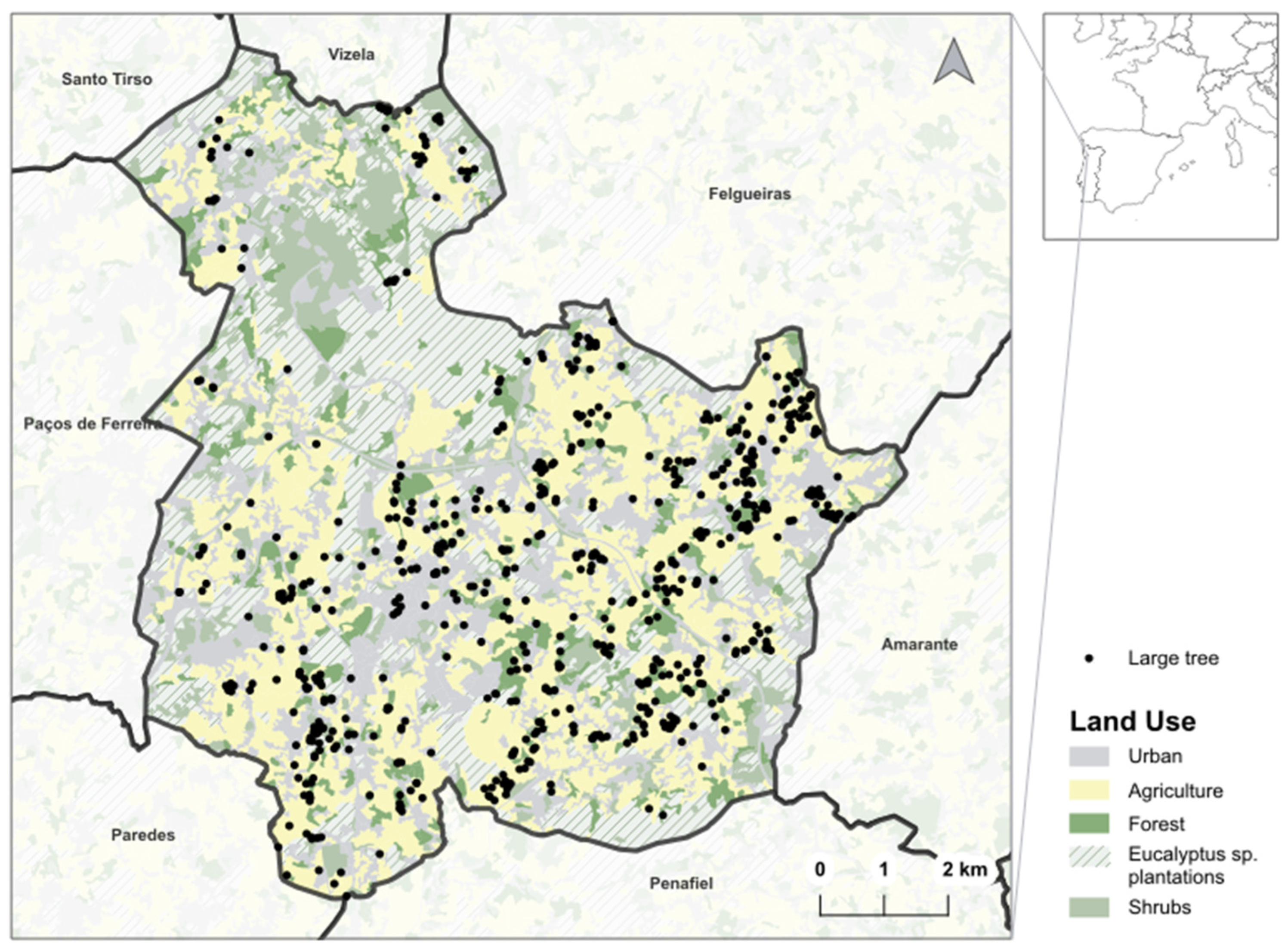
Figure 1. Geographical location of the study area in the municipality of Lousada, Portugal, and spatial distribution of the surveyed large trees (i.e., black dots—see Supplementary Information S1 for further details).
Remotesensing 18 01519 g001
Figure 2. Workflow used for satellite image time-series analysis to monitor tree loss, including data acquisition, pre-processing, breakpoint detection, post-validation of detected breaks and performance evaluation. Solid arrows represent the sequence of processing steps and associated data flows, while dotted arrows denote software-level interactions, such as feedback mechanisms or links between components.
Remotesensing 18 01519 g002
Figure 3. Descriptive summary of selected trees used in the break detection analysis evaluation, illustrating their structural variability. (a) Frequency distribution of species, grouped under “Others” if less than five individuals were recorded; (b) classification of trees by leaf phenology (deciduous vs. evergreen) and botanical class (angiosperm/deciduous vs. gymnosperm/evergreen); (c) distribution of diameter at breast height (DBH), with mean (dashed line) and ±1 standard deviation (dotted lines) marked in blue; (d) distribution of tree height with the same statistical markers (see Appendix A.1 for further details).
Remotesensing 18 01519 g003
Figure 4. Three examples of EVI2 time series (not deseasonalized) derived from the L2A product (2017–2025) with the best overall performance, illustrating distinct detection outcomes: (a) no breakpoint detected; (b) a true positive, in which a breakpoint was detected for a tree-felling event; and (c) a false positive associated with intensive tree pruning. The horizontal lines show the detected breakpoints for all algorithms/datasets and the long-term median validator. Black dots are the raw datapoints. The satellite images were compiled from Google Earth and show the same location from 2016 and August 2025.
Remotesensing 18 01519 g004
Figure 5. Circular histogram showing the relative frequency of detected break dates by month for felled trees in the field evaluation dataset. Break date assessment is based on pooling all methods across algorithms, pre-processing datasets, and validators that flagged valid breaks (N = 3658) (see Appendix A.2 for further details).
Remotesensing 18 01519 g005
Figure 6. Summary of average break detection performance across algorithms, EVI2 pre-processing methods, and validation strategies. Mean (±0.5 standard deviation) performance across five metrics (balanced accuracy, F1-score, sensitivity, specificity, precision) for (a) algorithms (cpm—change point model, ed—energy-divisive, wbs—wild-binary segmentation, stc—structural change in linear model, bfast01—breaks for additive season and trend model, (b) pre-processing dataset: MovWin (moving-window), Smo (Whittaker temporal smoothing), MovSmo (combined smoothing + windowing), and (c) post-breakpoint validation method: RandTrend (permutation-based trend test), LtMedComp (long-term median comparison), StMedComp (short-term median comparison). Factors are ranked in decreasing order of balanced accuracy. Appendix B.1, Appendix B.2 and Appendix B.3 present the detailed results of these graphics.
Remotesensing 18 01519 g006
Figure 7. Relative factor importance derived from random-effect variance decomposition of balanced accuracy. Variance estimates were corrected for factor cardinality to enable comparison among tree characteristics.
Remotesensing 18 01519 g007
Figure 8. Balanced accuracy across tree traits. Mean ± standard deviation are shown for (a) genus, structural attributes including (b) DBH and (c) height, (d) tree spatial context, (e) botanical class, and (f) leaf type. Grouping factors are presented in decreasing order of importance, from the most to the least influential.
Remotesensing 18 01519 g008
Disclaimer/Publisher’s Note: The statements, opinions and data contained in all publications are solely those of the individual author(s) and contributor(s) and not of MDPI and/or the editor(s). MDPI and/or the editor(s) disclaim responsibility for any injury to people or property resulting from any ideas, methods, instructions or products referred to in the content.