Abstract
Deep convective clouds, such as towering cumulus and Cumulonimbus, can endanger lives and property, also being a major hazard to aviation. This study presents the convective index (IndexCON) used operationally at the Portuguese Meteorological Watch Office. Moreover, IndexCON is evaluated against lightning and precipitation data for two years, between January 2022 and December 2023, over mainland Portugal and its surrounding areas. This index combines several European Center for Medium-Range Weather Forecasts (ECMWF) prognostic variables, such as stability indices, cloud water content, relative humidity and vertical velocity, using a fuzzy-logic approach. IndexCON performs well in the warm season (May–October), with a probability of detection (POD) of 70%, a false alarm ratio (FAR) of 30% and a probability of false detection (POFD) less than 5%, leading to a Critical Success Index (CSI) above 0.55. However, IndexCON performs worse in the cold season (November–April), when dynamical drivers are more relevant, mainly due to overestimating the convective activity, resulting in CSI and Heidke Skill Score (HSS) values below 0.3. Optimizing the membership functions partially reduces this overestimation. Finally, the added value of IndexCON was illustrated in detail for a thunderstorm episode, using satellite products, lightning and precipitation data.
1. Introduction
Deep convective clouds, namely Cumulonimbus (Cb) clouds, can cause lightning, hail, severe turbulence and icing [1], heavy precipitation and strong winds [2], and low-level wind shear associated with downbursts [1,3,4]. As Cb clouds commonly cause lightning and thunder, these clouds are sometimes referred to as thunderstorms [5]. Severe convective storms may also lead to the development of tornadoes [6,7,8] and/or waterspouts [7]. Thus, thunderstorms can jeopardize property, causing huge economic losses [8,9,10,11] and endangering animal and human lives [12,13,14,15]. For instance, lightning strikes cause 6000–24,000 deaths per year worldwide [12] and should be a concern when planning outdoor recreational activities [16,17].
Thunderstorms may also damage electrical infrastructure such as wind turbines [18] or power towers [2]. In addition, Cb clouds can also damage forests and crops [19], as well as trigger forest fires [20] and enhance their propagation [21,22]. In addition, thunderstorms can pose a major hazard to the transportation sector, especially to aviation [23,24], being responsible for several aviation accidents [1,4]. Furthermore, thunderstorm activity affects the air traffic control by constraining the usable part of the airspace, being therefore responsible for many flight delays [25]. In addition, the frequency of severe convective weather events is expected to increase throughout Europe until the end of the 21st century [26].
In mainland Portugal, thunderstorm activity has a bimodal distribution, with peaks in late spring and early autumn [27,28,29]. In contrast, in most areas of Europe, thunderstorms are more frequent from June to September [29,30], when the demand for air traffic is at its peak. Therefore, in order to mitigate the impact of Cbs on air traffic management, EUMETNET coordinates a European Cross Border Convective Advisory procedure. As part of this collaboration, between May and mid-October, 25 Meteorological Offices, including the Portuguese Institute for Sea and Atmosphere (IPMA), produce a convection risk forecast for the following day (D + 1) and an update for the current day [31]. In addition, aviation forecasters should provide forecasts to end-users containing not only information on convective cloud areas but also on the altitude of their tops [32]. Therefore, for all the reasons mentioned above, the accurate forecasting of these weather events is very important.
However, convective clouds are well known for their poor predictability [33,34] despite enormous advances in numerical weather prediction (NWP) models [35,36]. In addition, although operational regional NWP systems currently use a horizontal grid spacing of around 1–5 km, known as “convection-permitting models” [37], forecasting at convective scales faces several challenges, namely the demand for denser observation networks, a greater understanding of three-dimensional atmospheric turbulence, more sophisticated microphysical parameterizations and a more robust treatment of advection terms [37]. Therefore, forecasting the exact timing, location and severity of thunderstorms remains a challenge for operational forecasters and for the meteorological community in general.
Hence, several studies have been devoted to this subject, using different approaches, such as, Decision Trees [38], logistic regression [39], fuzzy logic algorithms [40], blending NWP ensembles [41] or blending observations with NWP outputs [42]. As the presence of atmospheric instability is considered a necessary condition for the development of deep convection [43], instability indices are frequently used as predictors [8,44,45,46,47,48,49]. Since the cloud electrification requires the coexistence of graupel, ice crystals and supercooled liquid water in the so-called charging zone [50,51], several forecasting algorithms have started to include microphysical model fields as lightning predictors [48,49,52], also based on ensemble prediction systems [53].
This article presents a new convective index, IndexCON, which has been used operationally at the Portuguese Meteorological Watch Office (MWO) since 2020. The main goal of IndexCON is to offer helpful information to aviation forecasters regarding the occurrence of convective clouds, namely cumulonimbus clouds or towering cumulus clouds. This index also provides information on the flight levels of cloud tops. IndexCON combines several prognostic variables (instability indices, cloud variables, relative humidity and vertical velocity) using a fuzzy logic approach. These variables are obtained from the European Center for Medium-Range Weather Forecasts (ECMWF).
The first goal of this article is to present IndexCON and its performance. The second objective is to discuss the strengths and shortcomings of this index, aiming to contribute to future developments in the prediction of the Cbs. The performance of IndexCON for lead times between 12 h and 35 h is evaluated against lightning and precipitation data over mainland Portugal and surrounding areas, for two years, between January 2022 and December 2023.
The paper is organized as follows: Section 2 describes the data used in this study. This section also explains IndexCON and the objective verification metrics. Section 3 presents the results of the objective verification and a case study that exemplifies the index performance. For this case study, Cb tops derived from IndexCON were also compared to the NWC SAF cloud top product. In addition, this study also evaluates other predictors, such as Convective Available Potential Energy (CAPE), Total Totals (TT), the K Index (KI), the surface Lifted Index (LIs) and the Jefferson (JEF) Index. Finally, Section 4 presents the discussion and the main conclusions are summarized in Section 5.
2. Data and Methods
2.1. Observation Data
This study uses observations for 2 years from January 2022 to December 2023. The precipitation and 10 m wind data, with a 10 min temporal resolution, are obtained from the IPMA network of surface weather stations (Figure 1). Reports of hail and tornadoes validated and provided by the European Severe Weather Database (ESSL, https://eswd.eu/) were also utilized. The quality control of these reports is explained in [7].
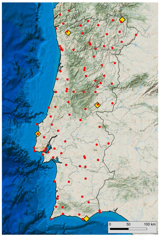
Figure 1.
IPMA weather stations (solid red circles) and LS7002 sensors (yellow diamonds) locations.
The lightning data are obtained from the network for the detection and localization of Atmospheric Electrical Discharges, operated by IPMA. This network is composed by five Advanced Lightning Sensor LS7002 (Vaisala [54]) located in Bragança/Aerodrome, Braga, Castelo Branco, Santa Cruz/Aerodrome, and Olhão. In addition, a TLP (Total Lightning Processor) system (Vaisala [55]) is installed at the IPMA headquarters in Lisbon. Furthermore, the process of detection and localization also benefits from the AEMET’s network in the western region of Spain [56]. The location of the sensors in mainland Portugal is shown in Figure 1.
This system has a detection efficiency greater than 90% for Cloud-to-Ground (CG) discharges and 50% for intra-cloud (IC) discharges [55]. The location accuracy depends on the distance between sensors and it varies between 250 m (minimum error) and more than 1 km near the southwest coast of mainland Portugal [56]. In the study region (described in Section 3.1), the location error is less than 1 km in 60% of occurrences (Figure S1 and Table S1). In addition, errors varying between 1 km and 5 km are found over the sea, mainly in the northwest area of the domain (not shown). The total lightning (CG and IC) accumulated in one hour is gridded on a regular 0.1° × 0.1° grid, which is the same as the NWP model grid.
This study also uses a half-hourly 4 km infrared (IR) brightness temperature (BT) dataset, developed by the National Oceanic and Atmospheric Administration (NOAA) and the National Centers for Environmental Prediction (NCEP), which is produced by merging the ~11 µm channel of five geostationary satellites to create a combined IR brightness temperature [57]. In addition, for the case study, the analysis of the Cb product is complemented with data from the cloud top height, which is obtained from the Satellite Applications Facility on Support to Nowcasting and Very Short-Range Forecasting (NWC SAF) software [58]. This product is derived from IR brightness temperature and estimates cloud top height by comparing observed and simulated IR brightness temperatures. The last output is obtained from the NWP’s vertical temperature and humidity profiles [58].
2.2. NWP Model Data and Forecasting Algorithm
The purpose of this section is to describe the convective index that was developed at the IPMA and has been operational at Portuguese Meteorological Watch Office since 2020. This index, named IndexCON, was developed to predict the Cumulonimbus potential and Cb top. This index uses hourly forecasts from the ECMWF global Integrated Forecasting System (IFS) deterministic model on a regular 0.1° × 0.1° grid.
The ECMWF model uses a sophisticated microphysics scheme with prognostic equations for cloud liquid and cloud ice condensate and for both rain and snow. The model uses 137 vertical levels, with the lowest level about 10 m above the ground and the vertical grid spacing increasing from 20 m near the surface to 290 m above 6 km in the troposphere. A complete description of the ECMWF/IFS model is available online (https://www.ecmwf.int/en/publications/ifs-documentation, accessed on 3 March 2024).
The IndexCON index uses fuzzy logic membership functions to integrate several predictors. This approach has been widely used in atmospheric science [40,59,60]. These functions range from 0 to 1 and determine the likelihood of an event occurring depending on a certain predictor. Williams [61] provides a very comprehensive description of this methodology.
In recent decades, the development of deep moist convection has been associated with static instability and low-level moisture [6,8,10,43]. Furthermore, Westermayer et al. [62] also revealed the importance of mid-troposphere moisture. Therefore, IndexCON predicts the occurrence of Cbs and their tops by blending several ingredients prone to deep moist convection, as detailed below. These ingredients also include cloud condensate, profiting from the fact that current NWP models explicitly predict these variables. Accordingly, IndexCON is defined as follows:
IndexCON = 100 FaCON × funml
The term FaCON diagnoses the presence of atmospheric instability by combining five indices, defined in Table 1. The funml intends to diagnose the presence of a cloud and is computed for each model level, as will be described in more detail ahead. Thus, IndexCON mimics the coexistence of atmospheric instability and clouds.
The chosen instability indices have been widely used to predict or diagnose an environment prone to thunderstorms [44,46,47,63], hail [64] or heavy precipitation [65,66] events. Furthermore, these indices have been used operationally by IPMA forecasters for more than two decades. The first three indices in Table 1 are based on temperature and humidity in two or three pressure levels and increase with the decreasing static stability in the layer 850–500 hPa and increasing moisture at 850 hPa. Jefferson and K index values also increase with increasing relative humidity at 700 hPa [46]. The last two indices are based on the lifted parcel theory, as explained in Table 1.

Table 1.
A summary of the static stability indices, Jefferson (JEF), Total Totals (TT), K index (KI), surface lifted index (LIs) and Convective Available Potential Energy (CAPE). T850, T700 and T500 represent the temperature at 850, 700 and 500 hPa, respectively. Td850 and Td700 are the dew-point temperatures at 850 and 700 hPa, respectively. Regarding the JEF index, θw850 is the wet-bulb potential temperature. In LIs, Tp500 is the 500 hPa temperature of a parcel lifted dry adiabatically from the surface to its condensation level and moist adiabatically thereafter. In the CAPE definition, is the virtual temperature of the parcel and is the virtual temperature of the environment. LFC is the level of free convection and EL is the equilibrium.
| Predictor | Definition | Reference |
|---|---|---|
| Jefferson | JEF = 1.60 θw850 − T500 − 0.5 (T700 − Td700) − 8 | [44,46,63,66] |
| Total Totals | TT = (T850 − T500) + (Td850 − T500) | [44,46,63,64,65,66] |
| K Index | KI = (T850 − T500) + Td850 − (T700 − Td700) | [44,46,63,66] |
| Lifted Index | LIs = T500 − Tp500 | [47,66] |
| CAPE | [8,46,47,65,67] |
The term FaCON also combines these instability indices with the total column cloud water content (tcl). As static instability is a necessary but not sufficient condition for deep convection, using tcl as a predictor aims to avoid high false alarm rates. Moreover, all predictors are combined using membership functions. Thus, FaCON is defined as
where Mtcl is the tcl membership function, which increases logarithmically with tcl and reaches a maximum value of 1 for tcl equal to 0.09 kg m−2, as shown in Figure 2.
FaCON = 0.1 facMIN + (0.1 facMAX) + (0.3 facMEAN) +
(0.35 (facMEAN × Mtcl)) + (0.15 (facMAX × Mtcl))
(0.35 (facMEAN × Mtcl)) + (0.15 (facMAX × Mtcl))
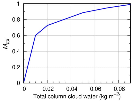
Figure 2.
Membership function of total column cloud water content (tcl).
In Equation (2), facMEAN, facMIN and facMAX depend on five membership functions (faJEF, faK, faTT, faLI and faCAPE), as follows:
facMEAN = 0.2 × faJEF + (0.2 × faK) + (0.2 × faTT) + (0.2 × faLI) + (0.2 × faCAPE)
facMIN = MIN(faJEF, faK, faTT, faLI, faCAPE)
facMAX = MAX(faJEF, faK, faTT, faLI, faCAPE)
The shape of the membership functions faJEF, faK, faTT, faLI and faCAPE depend on the five stability indices defined in Table 1, according to the expressions presented in Table 2 and shown in Figure 3. Figure 3a shows that faLI increases linearly as the LIs decreases for values of the LIs between 0 and −3 °C. The CAPE membership function, faCAPE, increases linearly with CAPE up to 250 J kg−1 when it reaches the maximum value of 1 (Figure 3a). faJEF and faTT increase linearly with the JEF and TT indices, at the same rate, reaching a maximum value of 1 when the JEF and TT indices reach 30 °C and 50 °C, respectively, (Figure 3b). faK rises more rapidly with K values, for K index values between 24 and 26 °C (Figure 3b). The range of values used in Table 2 is based on previous studies [46].
Table 2.
Expressions of the membership functions used in Equations (2)–(5).
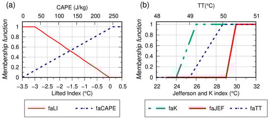
Figure 3.
Membership functions of CAPE and LIs (a) and JEF, TT and K (b) indices (see definition in Table 2).
Considering Equations (2)–(5), it is worth noting that, as facMIN represents the minimum value of the membership functions of the instability indices, FaCON can only reach its maximum value when all the membership functions diagnose static instability. Furthermore, FaCON can only reach its maximum value when a certain amount of cloud water content in the column (see Figure 2) coexists with atmospheric instability.
The function funml used in Equation (1) is computed for each model level and it uses a combination of fuzzy logic membership functions based on four ECMWF prognostic variables, namely, relative humidity (RH), the cloud liquid water mixing ratio (clw), the cloud ice water mixing ratio (ciw) and vertical velocity (ω), as follows:
where MRH is the RH membership function based on Morcrette et al. [60] (their Figure 2b), which assumes a value of 0 for RH below 60% and 1 for RH above 95%. In Equation (6), the three membership functions Mc-ln, Mc-lin and Mc-pol depend on the cloud water mixing ratio (cw = clw + ciw) but differ in the growth rate with cw, as shown in Figure 4a. The Mc-pol grows more slowly with cw, reaching a value of 1 when cw is equal to 0.4 g kg−1. The other two functions reach a value of 1 for cw equal to 0.08 g kg−1, but Mc-lin increases linearly (more slowly), while Mc-pol increases logarithmically with cw. The ω membership function Mω is based on Casqueiro et al. [68] (their Figure A1) and is shown in Figure 4b. Operationally, Equations (1) and (6) are applied to all model levels up to 150 hPa. Next, to ensure vertical consistency, the Cb top is defined as the maximum altitude where IndexCON ≥ 25 for a thickness of at least 13,000 feet (4 km). This will be exemplified in a case study presented in Section 3.3.
funml = 0.15 MRH + (0.3 Mc-ln) + [0.3 MAX(Mω, Mc-lin)] + (0.25 Mc-pol)
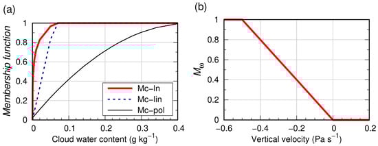
Figure 4.
Membership functions of (a) cloud water content and (b) vertical velocity, used in Equations (1) and (6) to define IndexCON.
2.3. Objective Verification Metrics
The use of contingency tables has been widely applied to the forecast’s evaluation [39,42,45,69], where forecasts and observations are expressed in binary terms. A simple 2 × 2 contingency table (Table 3) contains four elements, hits (A), false alarms (B), misses (C) and correct negatives (D), where A are the number of correctly predicted events; C denotes the number of events that occurred but were not predicted; B are the number of predictions of an event when the event was not observed; and D represents the number of times an event was not observed and not predicted.
Table 3.
A simple 2 × 2 contingency table, as in [44,46,70]. Note that, in some studies, the headings of “observation” and “forecast” may be transposed, as in [45]. Note that a “yes” forecast occurs when a given predictor exceeds (or is below) a certain threshold. The sample size is NN.
Several scores can be determined from a contingency table, as summarized in Table 4, such as the probability of detection (POD) defined as the fraction of observed events correctly predicted [42,44,45,46,47], and the probability of false detection (POFD), defined as the ratio of false alarms to the total numbers of nonevents [44], also known as the false alarm rate (FARate). Thus, FARate represents the probability of forecasting an event when it does not occur. In contrast, the False Alarm Ratio (FAR) is defined as the number of false alarms divided by the number of forecasted events or the fraction of “yes” forecasts that do not occur [70]. Thus, as discussed by Barnes et al. [70], the term false alarm rate should not be confused with the term false alarm ratio.
Table 4.
Skill scores and their definitions.
The three most commonly used scores for assessing the skill of a forecasting system in distinguishing between occurrences and non-occurrences are the Heidke Skill Score (HSS), the Critical Success Index (CSI) and the True Skill Score (TSS) [44,45,46]. For this reason, these scores were applied in the present study. However, Hogan et al. [69] discussed the weaknesses of these verification metrics, especially for low base rates, and proposed the use of the Symmetric Extreme Dependency Score (SEDS). Therefore, the SEDS has been employed in recent studies [69,71] and is also applied in the present study. In addition, this evaluation can be complemented by the F1 score (F1) [72]. All skill scores used are defined in Table 4.
Since TSS and HSS are frequently used, Haklander and Van Delden [44] proposed a new skill score, the Normalized Skill Score (NSS), defined as follows:
where is the maximum TSS value for a given threshold and is the maximum HSS for any threshold of a given predictor. Note that TSS and HSS may reach a maximum value for different thresholds. In order to incorporate the F1 score, which depends on POD and FAR [72], the optimal threshold () of each predictor is defined as follows:
where and are the thresholds that maximize the NSS and F1, respectively.
3. Results
3.1. Sample Characterization
The geographical distribution of lightning for the period 2022 to 2023 is presented in Figure 5, revealing that lightning activity is more frequent in the warm season (May–October) than in the cold season (November–April), especially over land, in line with previous studies [27,28,30]. Figure 5 also shows that in the warm season, the maximum frequency of lightning occurs in the northeast region, characterized by a complex topography, where the maximum number of days with lightning varies between 35 and 45. This reflects the importance of orographic forcing in triggering deep convection, as discussed in previous studies [73]. In contrast, in the cold season, the maximum thunderstorm activity is observed in coastal areas and over the sea. The lightning seasonal cycle for four regions is illustrated in Figure 5c, showing that in the northeast and central regions of mainland Portugal, thunderstorm activity has a bimodal distribution with a maximum in late spring and early summer (May and June) and a secondary maximum in September and October. In the Lisbon area and the southern region, lightning activity is mainly concentrated in September and October.
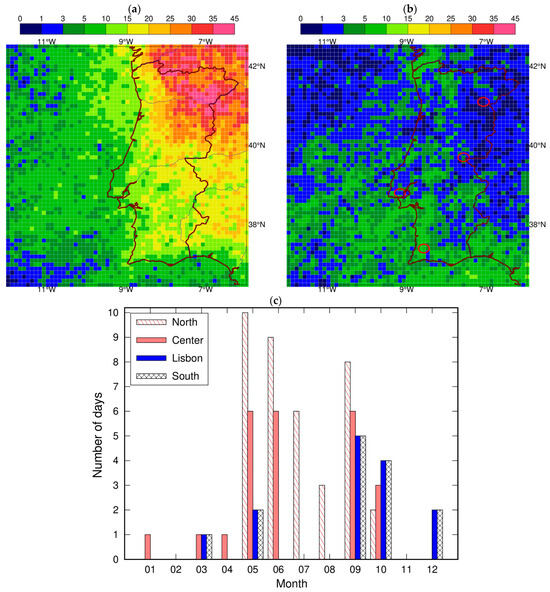
Figure 5.
The number of days with lightning discharges, on a regular 0.1° × 0.1° grid, for the years 2022 and 2023 for (a) the warm season and (b) cold season. (c) The monthly distribution of the days with lightning discharges for the four locations drawn in panel (b). The southernmost circle is named “south”, the northernmost circle is named “north”, the westernmost circle refers to “Lisbon” and the other is named “center”.
Figure 6 displays the spatial distribution of the days with a short-range heavy precipitation, hail and tornadoes reports. The threshold used to define an event of short-range heavy precipitation is 4 mm/10 min, which corresponds to 99th percentile of the 10 min precipitation for all stations (including only non-zero values) [74]. This figure reveals some similarities and some noteworthy differences between warm and cold seasons. For both seasons, heavy rainfall events were more frequent in the north of mainland Portugal, mainly near the coast. However, in the mountainous northeastern region, the frequency of heavy precipitation events is higher in the warm season than in the cold season. In the warm season, in this region, the maximum frequency of these events varies between 6 and 10 days. In addition, the hail reports were predominant in the mountainous region of northeastern Portugal, also in the warm season. In contrast, during the cold season, heavy precipitation events were concentrated mostly in northern coastal areas and the frequency of these events in the mountainous northeastern region was less than 4 days. In addition, tornadoes were more frequent in the cold season and at low altitudes, at a distance of less than 60 km from the coast. In the warm season, only one tornado was reported (see also Table 5). These results are in line with Leitão and Pinto [75], who showed that tornadoes in mainland Portugal occurred mainly from October to January, in association with cold fronts.
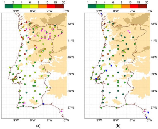
Figure 6.
The number of days with heavy precipitation events for the years 2022 and 2023 for (a) the warm season and (b) cold season. Hail and tornado events are marked with triangles and inverted triangles, respectively. The downburst event is marked with a diamond. Terrain elevations between 300 and 900 m and higher than 900 m are also depicted in cream and beige colors.
Table 5.
Reports of tornadoes, hail and downburst events for the period of 2022/2023 for the cold season and warm season (amount in parenthesis).
3.2. Evaluation of IndexCON Using Skill Scores
This section presents the results of the evaluation of the convective index, IndexCON, using the skill scores defined in Section 2.3. The objective verification was carried out using the hourly forecasts from the 1200 UTC analysis for lead times between 12 and 35 h. The criteria used to define a convective event based on the observations are presented in Table 6 and just one of the three criteria must be achieved to define a convective event. The lightning data for a given hour aggregates the lightning observations over a one-hour period centered on that hour. The used threshold for lightning was chosen bearing in mind that isolated CG flashes can cause damage to property and casualties [76]. For example, the forecast valid at 1200 UTC is compared to the lightning data observed between 1130 and 1230 UTC. Precipitation data refer to the maximum 10 min precipitation observed over a one-hour period.
Table 6.
Criteria used to define a convective event. In this study, the term convective event is used instead of thunderstorm because, in some cases, deep convection may not involve lightning (and the associated thunder). Some studies using these data sources for similar purposes are also listed.
Convective systems are known to have cold infrared (10.8µ or 10.7µ) BT, commonly used as a proxy of cloud top temperatures [77]. For instance, convective storms can have a BT ranging from 236 to 238 K in winter [77] and below 221 K in summer [10,78]. In the two years analyzed in this study, most lightning events were associated with BT ranging between 227 and 254 K in the warm season and between 235 and 261 K in the cold season (Table S2), in line with previous studies.
Therefore, when the surface observation network records no precipitation and no lightning, but the BT is below a certain threshold (typical of deep convection), this raises doubts about the possible occurrence of a convective event. Thus, these events were eliminated from the objective verification assessments. The threshold used was 221 K and 240 K in the warm and cold seasons, respectively. Using this criterium, 20890 and 260 events (nearly 5%) were removed from the verification sample, respectively, in the cold and warm seasons. As a result, the sample size (NN) is 533,207 and 397,000, respectively, for the warm and cold seasons. In addition, the frequency of the occurrence of a convective event (base rate) is 12.6% and 0.6% in the warm and cold seasons, respectively.
The skill scores of IndexCON, derived from the contingency tables using the criteria presented in Table 6, for both seasons, are shown in Figure 7, revealing that IndexCON’s performance in the warm season is considerably better than in the cold season. Figure 7a shows that, in the cold season, the NSS is approximately 0.8 for IndexCON between 25 and 40. For these thresholds, the POD varies between 53 and 68%, but the frequency bias is greater than 3, revealing an over-prediction of convective events. On the other hand, the HSS reaches maximum values for IndexCON between 55 and 70. The SEDS and F1 reach maximum values for this IndexCON range (not shown). Applying Equation (8), it is found that the optimum threshold for IndexCON is 45, which leads to a reduction in the frequency bias to 2.5 (not shown). For this threshold, the SEDS is nearly 0.6, and the HSS and F1 are approximately 0.28 (Figure 7b).
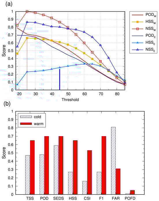
Figure 7.
IndexCON skill scores for the warm and cold seasons. (a) The POD, HSS and NSS as function of the IndexCON thresholds, where the subscripts w and c refer to the warm and cold seasons, respectively. The thin and thick vertical lines indicate the optimal threshold () defined by Equation (8), respectively, for warm and cold season; (b) various skill scores for threshold .
In the warm season, the NSS reaches a maximum value of 1 for IndexCON equal to 25, and above this threshold, the NSS sharply decreases (Figure 7a). Other metrics (the HSS, F1, SEDS and CSI) also reach the maximum values for IndexCON equal to 25. For this threshold, this index captures 70% of the convective events, and for values of IndexCON higher than 35, the probability of detection decreases sharply, attaining values of approximately 30% for IndexCON equal to 60. Figure 7 also reveals that in the warm season, IndexCON performs well, with an FAR of 0.3, SEDS equal to 0.7, CSI equal to 0.55, and HSS and TSS equal to 0.65.
3.3. Case Study
This section exemplifies the performance of IndexCON for one convective event. At 2100 UTC on 28 July 2024, as shown in Figure 8a, a depressionary system southwest of the Iberian Peninsula is present, very pronounced at mid-tropospheric levels, favoring southerly winds in the western Iberia region. At low levels, in the Gulf of Cadiz region, southeasterly winds promote the advection of very humid air towards the southern region of mainland Portugal, as illustrated by Figure 8b. This configuration favors conditions of strong instability (K index > 30 °C and CAPE > 1000 J kg−1) in western Iberia and the Gulf of Cadiz (Figure S2a,b) and moderate 0-6 km wind shear (between 10 and 20 m s−1) in southern Portugal and the Gulf of Cadiz (Figure S2c). The FaCON shows values above 0.7 in the southwest of the Iberian Peninsula and over the Gulf of Cadiz (Figure S3a). In the south of Portugal near the Spanish border, high FaCON values are due to the presence of large static instability, and over the Gulf of Cadiz, they reflect the coexistence of instability and tcl above 0.01 g kg−1 (Figures S2 and S3).
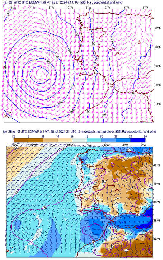
Figure 8.
ECMWF forecast valid at 2100 UTC on 21 July 2024, (a) 500 hPa geopotential height (dam) and wind (barbs), (b) 2 m dewpoint temperature and 925 hPa geopotential and wind (barbs).
Figure 9a shows that at 2100 UTC and in the next hour, IndexCON predicts a moderate risk of convective activity in the southwest of the Iberian Peninsula and over the Gulf of Cadiz. The comparison between IndexCON and the observed lightning activity reveals good agreement (Figure 9a–c). It is also worth noting that the area of convective activity displayed by IndexCON is considerably smaller than the area depicted by the other indicators (see Figures S2 and S3a). In addition, IndexCON provides a better prediction of the thunderstorm area, highlighted by the lightning observations and high tops (Figure 9a–c), than the other indicators. This illustrates the importance of combining FaCON and funml (see Section 2.2). At 2300 UTC on 28 July 2024, IndexCON discloses an expansion of the area of convective activity over southern Portugal, relative to the previous two hours, in agreement with the observations, despite an apparent slight time lag (Figure 9).
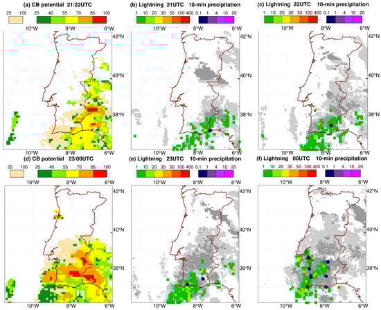
Figure 9.
Forecast of cumulonimbus potential (IndexCON), total lightning (CG + IC) and maximum 10 min precipitation observations. (a) IndexCON valid at 2100 UTC (shaded, green to red) and 2200 UTC (cream, shaded) on 28 July 2024. (b) Hourly lightning flashes on a regular 0.1° × 0.1° grid (shaded, green to red) and precipitation (0.1 to 20 mm/10 min) at 2100 UTC on 28 July 2024. Precipitation values in 10 min of less than or equal to 4 mm are marked with closed circles and those above are marked with a diamond. NWCSAF cloud tops above 320 hft (≈9.8 km) and 370 hft (≈11 km) are represented in light and dark gray, respectively. (c) The same as (b) but for 2200 UTC on 28 July 2024. (d) The same as (a) but for 2300 UTC on 28 July 2024 and 0000 UTC on 29 July 2024. (e) The same as (b) but for 2300 UTC on 28 July. (f) The same as (e) but for 0000 UTC on 29 July 2024.
Operationally, at the MWO, the top of the Cbs is expressed in Flight Level (FL), which is commonly used in aviation. An FL is a pressure altitude, expressed in hundreds of feet (hft) and is the height above the standard mean sea level pressure of 1013.25 hPa at which that pressure would occur in the ICAO standard atmosphere [32]. Therefore, it may not be the same as the actual altitude of the aircraft. In this document, as most readers are more familiar with altitude, tops are expressed in altitude.
Figure 10 shows the Cb top and the NWCSAF cloud top at 2100 and 2300 UTC on 28 July 2024. When comparing the two products, it is important to note that the NWCSAF product represents the top of all cloud types. On the other hand, the model Cb top represents the cloud top in areas where IndexCON exceeds 25, i.e., it depicts cloud tops exclusively in areas where cumulonimbus clouds are likely to occur. This explains the differences found over the sea to the west of the Iberian Peninsula. Apart from this, there is reasonable agreement between the areas where both products display cloud top altitudes above 300 hft. In these areas, the model predicts that cloud tops range between 350 hft and 400 hft, revealing a reasonable agreement with the NWCSAF product, except over a small area near the Spanish border, where the model underestimates the cloud top altitude by approximately 40 hft.
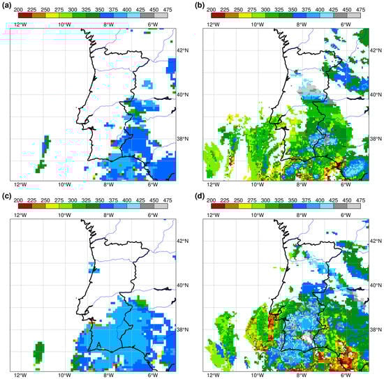
Figure 10.
(a) Forecast of altitude (in hft) of cumulonimbus top (based on IndexCON) and (b) NWCSAF cloud top, both valid at 2100 UTC on 28 July 2024. (c,d) Same as in (a,b) but for 2300 UTC. Forecasts based on 0000 UTC analysis.
Figure 11 displays the vertical profile of IndexCON at location A (in the south of mainland Portugal; see Figure 10c), showing that IndexCON exceeds 25 in the layer between 165 and 390 hft. As a result, the predicted cloud top altitude is 390 hft, slightly below the estimate from NWCSAF (≈400 hft). This index has maximum values in the layer between 330 and 380 hft, reflecting the presence of high relative humidity and cloud water content. Below 330 hft, the cloud water content is less than 0.015 g kg−1, but the vertical velocity varies between −0.5 and −1.6 Pa s−1 (not shown), and consequently, Mω is equal to 1 (see Figure 4b). Thus, in that layer, Mω plays a relevant role (see Equation (6)).
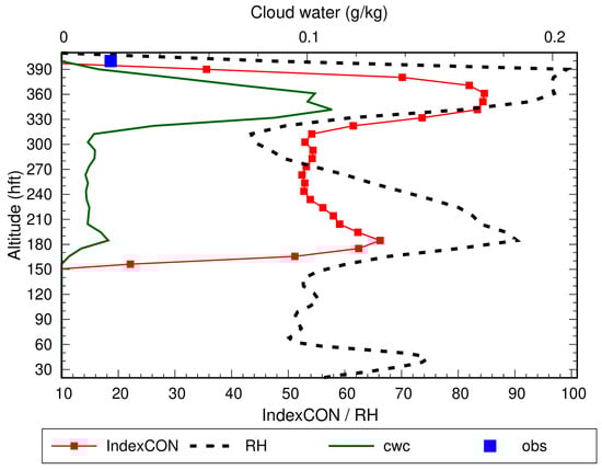
Figure 11.
Vertical profile of IndexCON, relative humidity (RH) and cloud water content (cwc) at location A shown in Figure 10c. The NWCSAF cloud top (in hft) is referred to as obs.
Over the next 24 h, the center of the depression propagated to the northeast (not shown). Accordingly, thunderstorms progressively moved north, affecting the southern and central regions of mainland Portugal during the morning (not shown) and the central and northern regions during the afternoon and evening of 29 July 2024 (Figure 12). During the afternoon (between 1500 and 1600 UTC), lightning activity is more intense than the night before and several stations registered precipitation, with a maximum value of 15.6 mm in 10 min in the northeast region, where lightning density is highest (Figure 12b,c). In this period, IndexCON overestimates the area of Cbs but correctly predicts high potential (above 85) for Cbs in the central and northeastern regions, despite displaying a slight shift westward in comparison to the thunderstorm areas (Figure 12a–c).
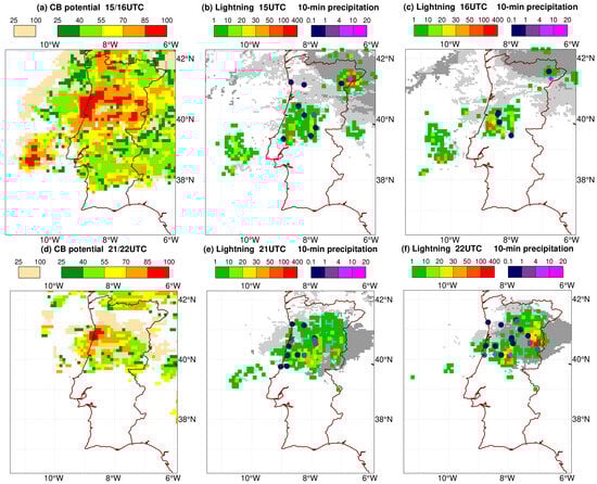
Figure 12.
Forecast of cumulonimbus potential (IndexCON), total lightning (CG + IC) and maximum 10 min precipitation observations. (a) IndexCON valid at 1500 UTC (shaded, green to red) and 1600 UTC (cream, shaded) on 29 July 2024. (b) Hourly lightning flashes on a regular 0.1° × 0.1° grid (shaded, green to red) and precipitation (0.1 to 20 mm/10 min) centered at 1500 UTC on 29 July 2024. Precipitation values in 10 min of less than or equal to 4 mm are marked with closed circles and those above are marked with a diamond. NWCSAF cloud tops above 320 hft (≈9.8 km) and 370 hft (≈11 km) are represented in light and dark gray, respectively. (c) The same as (b) but for 1600 UTC on 29 July 2024. (d) The same as (a) but for 2100 UTC and 2200 UTC on 29 July 2024. (e,f) The same as (b) but for 2100 UTC and 2200 UTC on 29 July 2024.
In the following hours, the Cb area predicted by IndexCON decreased (Figure 12d). At 2100 UTC, the comparison between observations and forecasts confirms the reduction in the Cb area, although the predicted area is slightly shifted to the southwest in comparison with the observations (Figure 12d–f). At this time, in the northeast region of mainland Portugal, the Cb product underestimates the altitude of the cloud tops since the model predicts cloud tops up to 375 hft and NWC SAF displays cloud tops between 325 and 450 hft (Figure S4). The analysis of a vertical profile (in the area) of relative humidity and cloud water content reveals that both variables decrease sharply for levels above 350–360 hft (Figure S5), justifying the IndexCON prediction of a cloud top at an altitude of 360 hft, while the NWC SAF estimates a cloud top at 410 hft. In addition, errors in the NWCSAF product might also contribute to this discrepancy since around 50% of the errors in the cloud top height product are greater than 500 m (16 hft) [58].
3.4. Evaluation of Other Predictors
This section analyzes the performance of the predictors defined in Table 1 and Table 2. In addition, it evaluates the skill of new membership functions. The comparison metrics of these predictors are summarized in Table 7 and Table 8, respectively, for warm and cold seasons. These tables show that the instability indices perform better in the warm season than in the cold season, except for the LIs. In the warm season, the Jefferson index and their membership functions are the best predictors, whereas the LIs and their membership functions are the worst. CAPE also performs poorly, especially in the cold season. This may be explained by the fact that the majority of the convective events occur with low CAPE (Figure S6). In particular, in the cold season, more than 80% of convective events occurred for CAPE below 200 J kg−1 (not shown).
Table 7.
Skill scores of several predictors for the threshold (see Equation (8)) for the warm season. The new membership functions are identified by subscript n.
Table 8.
Skill scores of several predictors for the threshold (see Equation (8)) for the cold season. The new membership functions are identified by subscript n.
Table 7 and Table 8 also show that applying a membership function based on CAPE leads to an increase in forecasting performance. For example, in the cold season, the SEDS of CAPE is less than 0.45, while the SEDS of faCAPE is approximately 0.6 (Table 8). This improvement illustrates the potential benefit of using membership functions instead of a fixed threshold for a given predictor. To this end, it is necessary that the membership function reasonably reflects the predictor conditional probability curve [42]. For example, the CAPE conditional probability curve shows that the probability of a convective event occurring increases with CAPE, reaching a maximum (less than 0.5) for CAPE of approximately 175 J kg−1. For higher CAPE values, it remains below 0.5 (Figure 13a). As the CAPE membership function reasonably matches the conditional probability curve, no new functions were tested.
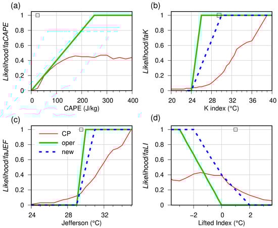
Figure 13.
Conditional probability (CP) curves of four instability indices for the convective events (the red solid line) for (a) CAPE, (b) the K index, (c) the Jefferson index, and (d) LIs. The old operational (oper) and new functions are represented by thick solid and dashed lines, respectively. The threshold that maximizes the scores of each index is marked by an open square. The CP curves are determined from the relative frequency of convective events for a given interval of a specific parameter.
A comparison between the conditional probability curves and the operational membership functions for the other stability indices shows that these functions could be optimized (Figure 13b–d and Figure S7). The new functions for Jefferson and KI are similar to the old operational functions, except the new functions increase more gradually, more accurately reflecting the conditional probability curves (Figure 13b,c). For instance, the old faK increases sharply for the K index between 24 and 26 °C, whereas the new faK (faKn) increases gradually for the K index between 24 and 30 °C, adjusting better to the conditional probability curve of the K index. As a result, the use of the new function for the K index leads to a smaller overestimation (lower BIAS) than the old function, having a positive impact on the forecasting performance, visible in terms of an increase in the SEDS, CSI, HSS and F1 score, for both seasons (Table 7 and Table 8). The new Jefferson membership function outperforms the operational version, especially in the cold season.
As far as LIs are concerned, the operational LIs membership function (faLI) takes the value zero for LIs ≥ 0 °C. In contrast, the new function (faLIn) increases between 0 and 0.4 for decreasing values of LIs in the range 0 to 2 °C, better adjusting to the LIs conditional probability curve (Figure 13d) and LIs distribution (Figure S6). For negative values of LIs, the new version increases more rapidly as LIs decrease, reaching a maximum value for LIs equal to −2 °C rather than for LIs equal to −3 °C (Figure 13d). Therefore, the new membership function drives improvements in performance, especially in the warm season, as evidenced by the skill scores, despite some overestimation.
With regard to TT, this index performs reasonably well in the warm season but poorly in the cold season due to a strong tendency to overestimate Cb occurrences (Table 7 and Table 8). The TT conditional probability curve shows that the likelihood of a convective event occurring increases with TT for values above 46 °C, reaching a maximum (≈0.6) for TT equal to 51.5 °C (Figure S7). This suggests that the TT membership function should vary more gradually with TT than the operational version. Thus, a new function (faTTn) that increases more slowly with TT is tried (Figure S7). This new function outperforms faTT in the warm season (with a higher TSS, as seen in Table 7) but has a marginal impact in the cold season (not shown).
It is worth noting that, as Lin et al. [40] mentioned, there is some subjectivity and simplification in creating the membership functions, so the correspondence between the conditional probability curves and the membership functions may not be perfect. So, although the conditional probability curves of Jefferson, KI and TT indices suggest that their membership functions should be more gradual (Figure 13), these are not implemented to avoid excessively reducing the probability of detection since none of these functions are the only Cb predictors.
3.5. Evaluation of FaCON
In IndexCON, the FaCON term, which depends only on two-dimensional fields, plays a key role. Therefore, this section presents an evaluation of the old and new versions of FaCON. As four membership functions (faJEFn, faKn, faTTn and faLIn) outperformed the old functions, these new functions were applied to Equations (3)–(5) derive a new version of FaCON (FaCONn). Moreover, in facMEANn (the new facMEAN), the weights assigned to each function are based on the skill scores of each function for each season as follows:
where the relative weights (C1 to C5) given to each of the membership functions are presented in Table 9 and depend on the SEDS, TSS and HSS as follows:
facMEANn = c1 × faJEFn + (c2 × faKn) + (c3 × faTTn) + (c4 × faLIn) + (c5 × faCAPE)
Table 9.
Relative weights given to the membership functions used in FaCON (Equation (2)).
Figure 14 presents the old and new FaCON scores, showing that the implementation of the new membership functions improves the SEDS and reduces the FAR. This improvement is also noticeable in the HSS and CSI scores (Figure S8) and is more pronounced in the cold season.
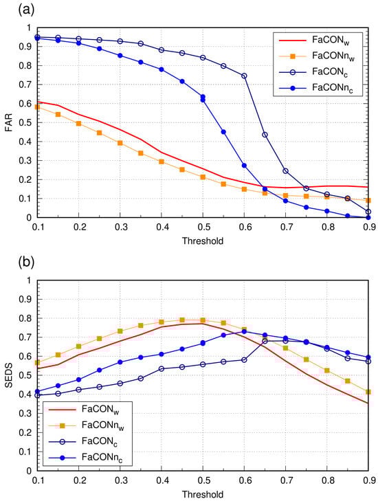
Figure 14.
The FAR (a) and SEDS (b) of the old and new FaCON (FaCONn) as a function of the thresholds. Subscripts w and c refer to the warm and cold seasons, respectively.
4. Discussion
The convective index, IndexCON, operational at the IPMA, is derived from the forecasts of the ECMWF deterministic model, using various prognostic variables such as Jefferson (JEF), Total Totals (TT), K index (KI), surface lifted index (LIs), Convective Available Potential Energy (CAPE), cloud water content, relative humidity and vertical velocity. These variables are combined using a fuzzy logic approach instead of fixed thresholds. These functions range from 0 to 1 and determine the likelihood of a convective event.
IndexCON forecasts, for forecast ranges between 12 and 35 h, were evaluated against lightning and precipitation observations for mainland Portugal and surrounding areas. In addition, validated ESSL reports of hail and tornadoes were also used to define a convective event. This assessment was carried out, using skill scores, for the warm season (May–October) and cold season (November–April) for two years between January 2022 and December 2023.
The results show that IndexCON performs well in the warm season, with a POD of 70% and FAR of 30%. Furthermore, a detailed analysis of a thunderstorm episode in July 2024 (Figure 8, Figure 9, Figure 10, Figure 11 and Figure 12) reveals good agreement between the areas of high cloud tops (altitudes above 320 hft) based on IndexCON and the cloud tops from NWC SAF, illustrating the usefulness of this product for validation purposes. Thus, this comparison should be extended to a longer period.
In the cold season, IndexCON tends to overpredict the occurrence of convective events, with an FAR of around 0.8 (Figure 7). In addition, for the optimal threshold, the IndexCON’s probability of detection is around 50% in this season. The skill scores of the predictors used in IndexCON reveal that some predictors perform considerably worse than others. Therefore, the weight assigned to each predictor should reflect this fact. In addition, certain membership functions misrepresent the shape of the probability distribution of some instability indices, leading to a considerable overestimation of convective events. Addressing these deficiencies reduces the overestimation of convective phenomena and improves the forecasting skill of FaCON, a key component of IndexCON (Figure 14).
The IndexCON’s poorer performance in the cold season may also be explained by other factors. In the mid-latitudes, convective activity in winter differs to summer for several reasons [79]. In summer, the tropopause lies at 14 to 16 km altitude and drops to 7 to 9 km in winter. Therefore, in winter, convective clouds are confined to a depth about half of that of summer. In addition, the −10 °C temperature level, where charge separation is very efficient, is closer to the surface in the cold season [79,80]. This causes a reduction in the updraft velocity near this level and lowers the charge separation rate. As a result, in the cold season, convective clouds may exhibit very low electrical activity or none [80]. Moreover, recently, Morgenstern et al. [81] analyzed the thunderstorm environment over Europe and found two major thunderstorm environments. The first type, named mass-field thunderstorm, characterized by moderate or large CAPE, large values of dewpoint temperatures at 2 m and high −10 °C isotherm height, corresponds to the archetypal thunderstorm environment generally described in the literature [10,43]. This mass-field thunderstorm is predominant in the warm season and is most important in continental Europe.
The other major thunderstorm environment, the wind-field thunderstorm, is associated with strong winds and high wind shear and originates from more diverse meteorological conditions than the mass-field thunderstorm. The wind-field thunderstorms are predominant in the cold season, especially in winter and over sea [81]. These results support the hypothesis that high wind shear creates tilted clouds (Figure 7 of Kitagawa [80]), favoring large distances between the charge centers, which may be sufficient to produce lightning [79], even in shallow clouds in low CAPE environments [81]. Therefore, in the cold season, CAPE and other instability indices may be poor predictors. In line with these results, Clark [82] also documented an outbreak of tornadoes that affected southern England in December 2006 in an environment of meager CAPE (<100 J kg−1) and high wind shear.
It is also worth noting that errors in the temperature profile and/or near-surface humidity can lead to a large underestimation of CAPE [67]. This may partly explain the fact that a large percentage (80%) of thunderstorms occurred with CAPE below 250 J kg−1 and that the membership functions of other instability indices (Jefferson or K index) outperformed the CAPE membership function in the warm season (Table 7). In addition, the effect of neglecting the virtual temperature correction in the CAPE calculation may be substantial in meager CAPE environments [83]. Hence, the CAPE computation in ECMWF was revised to include this correction [67], and this new version began to be used operationally at the IPMA in January 2024.
For the above reasons, it is understandable that IndexCON performs better in the warm season when thermodynamic factors predominate over dynamic drivers. In the future, the focus should be on improving IndexCON in the cold season, bearing in mind that although lightning activity is higher in the warm season, tornadic storms are more frequent in mainland Portugal in the cold season [75], and during winter, there is the added danger of CG lightning causing personal injury [76] or damage to structures on the ground [18,76].
Furthermore, as the shallower convective clouds during the cold season may have little to no lightning activity, lightning observations may lead to an under-detection of convective activity, partly contributing to IndexCON’s high false alarm ratio. Moreover, ground-based detection networks have a low detection rate of intra-cloud lightning [55]. Thus, in the future, the systematic utilization of radar data, for instance, as in Ripesi [84], to evaluate convective NWP-based products will be a significant step forward, especially in the cold season.
The IndexCON accuracy is expected to be limited by the quality of the model variables. For example, Taszarek et al. [85] evaluated various reanalysis-derived convective parameters against radiosonde data over Europe and North America and showed that reanalysis tend to underestimate low-level moisture, CAPE and wind shear. Thus, in a forthcoming study, it would be interesting to assess the performance of IndexCON based on different data sources, such as radiosonde or reanalysis data.
The area of this study is limited to mainland Portugal and its surrounding areas, although IndexCON is used operationally over the Portuguese Flight Information Regions, which cover an area of around 6 million km2 (Figure 1 of [71]). In the future, it will be advisable to extend this assessment to a wide area, benefiting from the products of the Meteosat Third Generation (MTG) satellite and, in particular, the lightning data [86]. This would permit an assessment of IndexCON’s applicability to other regions.
5. Conclusions
This study presents and evaluates the performance of a new convective index (IndexCON). This evaluation was performed for two years between January 2022 and December 2023 over mainland Portugal and its surrounding areas. IndexCON forecasts (for steps ranging from 12 to 35 h) were evaluated against lightning and precipitation observations. In addition, validated ESSL reports of hail and tornadoes were also used to define a convective event. It was found that IndexCON has good performance in the warm season (May–October), when thermodynamical drivers play a key role, with a probability of detection (POD) of 70% and a false alarm ratio (FAR) less than 30%. In contrast, in the cold season (November–April), when dynamical drivers (such as frontogenesis processes) are more relevant, IndexCON performs worse with a lower POD and smaller CSI values and HSSs. In addition, it tends to over-predict the occurrence of convective events, with an FAR of around 0.8. As lightning activity associated with convective clouds is lower in the cold season than in the warm season, using radar or new MTG satellite data to complement the evaluation procedure will be beneficial. Moreover, additional parameters, such as wind shear, could be included in the future.
Supplementary Materials
The following supporting information can be downloaded at: https://www.mdpi.com/article/10.3390/rs17091627/s1, Figure S1: Absolute frequency of location error for the lightning network over the domain shown in Figure 5a. The range of the frequency intervals is 250 m; Figure S2: ECMWF forecast (H+21) valid at 2100UTC on 28 July 2024, for (a) K index (in °C), (b) CAPE (J kg−1) and (c) 0-6 km bulk wind shear (m s−1), which is the vector difference between the 10 m wind and the 6 km wind; Figure S3: ECMWF forecast (H+21) valid at 2100UTC on 28 July 2024, for (a) FaCON and (b) tcl; Figure S4: (a) Forecast of altitude (in hft) of Cumulonimbus top (based on IndexCON) and (b) NWCSAF cloud top, both valid at 2100UTC on 29 July 2024. Forecast based on 0000UTC analysis; Figure S5: Vertical profiles of IndexCON, relative humidity (RH, in %) and cloud water content (cwc) at location B, marked in Figure S4a; Figure S6: Relative frequency of occurrence of several predictors for convective events (C) and non-convective events (No), represented as thick bars in light orange and thin bars in blue, respectively. Figure S7: Conditional probability (CP) curve of Total-Totals (TT) for the convective events. The old operational (oper) and new functions are represented by thick solid and dashed lines, respectively. The threshold of TT that maximizes the skill scores is marked as open square; Figure S8: HSS (a) and CSI (b) of the old and new FaCON (FaCONn) as a function of the thresholds. Subscripts w and c refer to the warm and cold seasons, respectively. Table S1: Relative frequency of location error for the lightning network over the domain shown in Figure 5a; Table S2: Minimum, 25 percentiles (25p), mean and 75 percentiles (75p) of IR10.7 brightness temperature (in Kelvin) for lightning events, for both warm and cold seasons.
Funding
This research received no external funding.
Data Availability Statement
The precipitation and lightning data can be requested on the official website of the Portuguese Weather Service (IPMA—https://www.ipma.pt/en/siteinfo/contactar.jsp, accessed on 3 March 2024). The NOAA/NCEP half-hourly 4 km merged IR brightness temperature dataset is available at https://disc2.gesdisc.eosdis.nasa.gov/data/MERGED_IR/GPM_MERGIR.1/, accessed on 14 October 2024).
Acknowledgments
Many thanks to Isabel Soares for the discussions and support concerning lightning data. Thanks to Emanuel Dutra for processing the NWC SAF cloud top height product. I would like to thank the three anonymous reviewers for their constructive suggestions that contributed to improving the article.
Conflicts of Interest
The author declares no conflicts of interest.
References
- Tafferner, C.; Forster, M.; Hagen, T.; Hauf, B.; Lunnon, A.; Mirza, Y.; Guillou, T.; Zinner, T. Improved thunderstorm weather information for pilots through ground and satellite based observing systems. In Proceedings of the 14th Conference on ARAM, 90th AMS Annual Meeting 2010, Atlanta, GA, USA, 17–21 January 2010. [Google Scholar]
- Pinto, P.; Belo-Pereira, M. Damaging Convective and Non-Convective Winds in Southwestern Iberia during Windstorm Xola. Atmosphere 2020, 11, 692. [Google Scholar] [CrossRef]
- Sinclair, P.C.; Kuhn, P.M. Aircraft Low Altitude Wind Shear Detection and Warning System. J. Appl. Meteorol. Climatol. 1991, 30, 3–16. [Google Scholar] [CrossRef]
- McCarthy, J.; Serafin, R.; Wilson, J.; Evans, J.; Kessinger, C.; Mahoney, W.P., III. Addressing the Microburst Threat to Aviation: Research-to-Operations Success Story. Bull. Am. Meteorol. Soc. 2022, 103, E2845–E2861. [Google Scholar] [CrossRef]
- Phillips, V.T.J.; Formenton, M.; Kanawade, V.P.; Karlsson, L.R.; Patade, S.; Sun, J.; Barthe, C.; Pinty, J.-P.; Detwiler, A.G.; Lyu, W.; et al. Multiple Environmental Influences on the Lightning of Cold-Based Continental Cumulonimbus Clouds. Part I: Description and Validation of Model. J. Atmos. Sci. 2020, 77, 3999–4024. [Google Scholar] [CrossRef]
- Schumacher, P.N.; Boustead, J.M. Mesocyclone Evolution Associated with Varying Shear Profiles during the 24 June 2003 Tornado Outbreak. Weather Forecast. 2011, 26, 808–827. [Google Scholar] [CrossRef]
- Groenemeijer, P.; Kühne, T. A Climatology of Tornadoes in Europe: Results from the European Severe Weather Database. Mon. Weather Rev. 2014, 142, 4775–4790. [Google Scholar] [CrossRef]
- Belo-Pereira, M.; Andrade, C.; Pinto, P. A long-lived tornado on 7 December 2010 in mainland Portugal. Atmos. Res. 2017, 185, 202–215. [Google Scholar] [CrossRef]
- Hammer, T.W.; Schmidlin, T.W. Response to Warnings during the 3 May 1999 Oklahoma City Tornado: Reasons and Relative Injury Rates. Weather Forecast. 2002, 17, 577–581. [Google Scholar] [CrossRef]
- Kunz, M.; Blahak, U.; Handwerker, J.; Schmidberger, M.; Punge, H.J.; Mohr, S.; Fluck, E.; Bedka, K.M. The severe hailstorm in southwest Germany on 28 July 2013: Characteristics, impacts and meteorological conditions. Q. J. R. Meteorol. Soc. 2018, 144, 231–250. [Google Scholar] [CrossRef]
- Púčik, T.; Castellano, C.; Groenemeijer, P.; Kühne, T.; Rädler, A.T.; Antonescu, B.; Faust, E. Large Hail Incidence and Its Economic and Societal Impacts across Europe. Mon. Weather Rev. 2019, 147, 3901–3916. [Google Scholar] [CrossRef]
- Holle, R. A Summary of Recent National-Scale Lightning Fatality Studies. Weather Clim. Soc. 2016, 8, 35–42. [Google Scholar] [CrossRef]
- Cerveny, R.S.; Bessemoulin, P.; Burt, C.C.; Cooper, M.A.; Cunjie, Z.; Dewan, A.; Finch, J.; Holle, R.L.; Kalkstein, L.; Kruger, A.; et al. WMO Assessment of Weather and Climate Mortality Extremes: Lightning, Tropical Cyclones, Tornadoes, and Hail. Weather Clim. Soc. 2017, 9, 487–497. [Google Scholar] [CrossRef]
- Mills, B. An Updated Assessment of Lightning-Related Fatality and Injury Risk in Canada: 2002–2017. Nat. Hazards 2020, 102, 997–1009. [Google Scholar] [CrossRef]
- Bingert, R.; Bremer, L.; Büttner, A.; Nigbur, S.; Blumenthal, R.; Zack, F. A 15-year review of lightning deaths in Germany—With a focus on pathognomonic findings. Int. J. Legal Med. 2024, 138, 1343–1349. [Google Scholar] [CrossRef] [PubMed]
- Walsh, K.M.; Bennett, B.; Cooper, M.A.; Holle, R.L.; Kithil, R.; López, R.E. National athletic trainers’ association position statement: Lightning safety for athletics and recreation. J. Athl. Train. 2000, 35, 471–777. [Google Scholar] [CrossRef]
- Ströhle, M.; Wallner, B.; Lanthaler, M.; Rauch, S.; Brugger, H.; Paal, P. Lightning accidents in the austrian alps—A 10-year retrospective nationwide analysis. Scand. J. Trauma Resusc. Emerg. Med. 2018, 26, 74. [Google Scholar] [CrossRef]
- Matsui, M.; Michishita, K.; Yokoyama, S. Cloud-to-Ground Lightning Flash Density and the Number of Lightning Flashes Hitting Wind Turbines in Japan. Electr. Power Syst. Res. 2020, 181, 106066. [Google Scholar] [CrossRef]
- Gobbo, S.; Ghiraldini, A.; Dramis, A.; Dal Ferro, N.; Morari, F. Estimation of Hail Damage Using Crop Models and Remote Sensing. Remote Sens. 2021, 13, 2655. [Google Scholar] [CrossRef]
- Menezes, L.S.; Russo, A.; Libonati, R.; Trigo, R.M.; Pereira, J.M.; Benali, A.; Ramos, A.M.; Gouveia, C.M.; Rodriguez, C.A.M.; Deus, R.; et al. Lightning-induced fire regime in Portugal based on satellite-derived and in situ data. Agric. For. Meteorol. 2024, 355, 110108. [Google Scholar] [CrossRef]
- Johnson, R.H.; Schumacher, R.S.; Ruppert, J.H.; Lindsey, D.T.; Ruthford, J.E.; Kriederman, L. The Role of Convective Outflow in the Waldo Canyon Fire. Mon. Weather Rev. 2014, 142, 3061–3080. [Google Scholar] [CrossRef]
- Pinto, P.; Silva, Á.; Viegas, D.; Almeida, M.; Raposo, J.; Ribeiro, L. Influence of Convectively Driven Flows in the Course of a Large Fire in Portugal: The Case of Pedrógão Grande. Atmosphere 2022, 13, 414. [Google Scholar] [CrossRef]
- Gultepe, I.; Sharman, R.; Williams, P.D.; Zhou, B.; Ellrod, G.; Minnis, P.; Trier, S.; Griffin, S.; Yum, S.S.; Gharabaghi, B.; et al. Review of High Impact Weather for Aviation Meteorology. Pure Appl. Geophys. 2019, 176, 1869–1921. [Google Scholar] [CrossRef]
- Taszarek, M.; Kendzierski, S.; Pilguj, N. Hazardous weather affecting european airports. Weather Clim. Extrem. 2000, 28, 100243. [Google Scholar] [CrossRef]
- Ahlstrom, U. Work domain analysis for air traffic controller weather displays. J. Saf. Res. 2005, 36, 159–169. [Google Scholar] [CrossRef]
- Rädler, T.; Groenemeijer, P.H.; Faust, E.; Sausen, R.; Púcik, T. Frequency of severe thunderstorms across Europe expected to increase in the 21st century due to rising instability. Npj Clim. Atmos. Sci. 2019, 2, 1–5. [Google Scholar] [CrossRef]
- Ramos, M.; Sousa, P.; Trigo, R.M.; Janeira, M.; Prior, V. Cloud to ground lightning activity over Portugal and its association with circulation weather types. Atmos. Res. 2011, 101, 84–101. [Google Scholar] [CrossRef]
- Santos, J.A.; Reis, M.A.; Sousa, J.; Leite, S.M.; Correia, S.; Janeira, M.; Fragoso, M. Cloud-to-ground lightning in Portugal: Patterns and dynamical forcing. Nat. Hazards Earth Syst. Sci. 2012, 12, 639–649. [Google Scholar] [CrossRef]
- Taszarek, M.; Allen, J.; Púčik, T.; Groenemeijer, P.; Czernecki, B.; Kolendowicz, L.; Lagouvardos, K.; Kotroni, V.; Schulz, W. A Climatology of Thunderstorms across Europe from a Synthesis of Multiple Data Sources. J. Clim. 2019, 32, 1813–1837. [Google Scholar] [CrossRef]
- Poelman, R.; Schulz, W.; Diendorfer, G.; Bernardi, M. The european lightning location system EUCLID—Part 2: Observations. Nat. Hazards Earth Syst. Sci. 2016, 16, 607–616. [Google Scholar] [CrossRef]
- Eurocontrol. Summer 2023: High Weather Impacts on the Network. In Eurocontrol European Aviation Trends; Eurocontrol: Brussels, Belgium, 2023. [Google Scholar]
- ICAO. Annex 3 to the Convention on International Civil Aviation, International Standards and Recommended Practices, 20th ed.; International Civil Aviation Organization: Montreal, QC, Canada, 2018; pp. 29–186. [Google Scholar]
- Walser, D.; Lüthi, D.; Schär, C. Predictability of precipitation in a cloud-resolving model. Mon. Weather Rev. 2004, 132, 560–577. [Google Scholar] [CrossRef]
- Keil, C.; Heinlein, F.; Craig, G.C. The convective adjustment time-scale as indicator of predictability of convective precipitation. Q. J. R. Meteorol. Soc. 2014, 140, 480–490. [Google Scholar] [CrossRef]
- Bauer, P.; Thorpe, A.; Brunet, G. The quiet revolution of numerical weather prediction. Nature 2015, 525, 47–55. [Google Scholar] [CrossRef] [PubMed]
- Bengtsson, L.; Andrae, U.; Aspelien, T.; Batrak, Y.; Calvo, J.; de Rooy, W.; Gleeson, E.; Hansen-Sass, B.; Homleid, M.; Hortal, M.; et al. The HARMONIE–AROME Model Configuration in the ALADIN–HIRLAM NWP System. Mon. Weather Rev. 2017, 145, 1919–1935. [Google Scholar] [CrossRef]
- Yano, J.I.; Ziemiański, M.Z.; Cullen, M.; Termonia, P.; Onvlee, J.; Bengtsson, L.; Carrassi, A.; Davy, R.; Deluca, A.; Gray, S.L.; et al. Scientific Challenges of Convective-Scale Numerical Weather Prediction. Bull. Am. Meteorol. Soc. 2018, 99, 699–710. [Google Scholar] [CrossRef]
- Mills, G.A.; Colquhoun, J.R. Objective Prediction of Severe Thunderstorm Environments: Preliminary Results Linking a Decision Tree with an Operational Regional NWP Model. Weather Forecast. 1998, 13, 1078–1092. [Google Scholar] [CrossRef]
- Flora, M.L.; Potvin, C.K.; Skinner, P.S.; Handler, S.; McGovern, A. Using Machine Learning to Generate Storm-Scale Probabilistic Guidance of Severe Weather Hazards in the Warn-on-Forecast System. Mon. Weather Rev. 2021, 149, 1535–1557. [Google Scholar] [CrossRef]
- Lin, P.; Chang, P.; Jou, B.J.-D.; Wilson, J.W.; Roberts, R.D. Objective Prediction of Warm Season Afternoon Thunderstorms in Northern Taiwan Using a Fuzzy Logic Approach. Weather Forecast. 2012, 27, 1178–1197. [Google Scholar] [CrossRef]
- Bouttier, F.; Marchal, H. Probabilistic thunderstorm forecasting by blending multiple ensembles. Tellus A 2020, 72, 1–19. [Google Scholar] [CrossRef]
- Müller, R.; Barleben, A. Data-Driven Prediction of Severe Convection at Deutscher Wetterdienst (DWD): A Brief Overview of Recent Developments. Atmosphere 2024, 15, 499. [Google Scholar] [CrossRef]
- Mcnulty, R.P. Severe and Convective Weather: A Central Region Forecasting Challenge. Weather Forecast. 1995, 10, 187–202. [Google Scholar] [CrossRef]
- Haklander, J.; Delden, A.V. Thunderstorm predictors and their forecast skill for the Netherlands. Atmos. Res. 2003, 67–68, 273–299. [Google Scholar] [CrossRef]
- Lee, R.R.; Passner, J.E. The Development and Verification of TIPS: An Expert System to Forecast Thunderstorm Occurrence. Weather Forecast. 1993, 8, 271–280. [Google Scholar] [CrossRef]
- Kunz, M. The Skill of convective parameters and indices to predict isolated and severe thunderstorms. Nat. Hazards Earth Syst. Sci. 2007, 7, 327–342. [Google Scholar] [CrossRef]
- Vujović, D.; Paskota, M.; Todorović, N.; Vučković, V. Evaluation of the stability indices for the thunderstorm forecasting in the region of Belgrade, Serbia. Atmos. Res. 2015, 161–162, 143–152. [Google Scholar] [CrossRef]
- Yair, Y.; Lynn, B.; Price, C.; Kotroni, V.; Lagouvardos, K.; Morin, E.; Mugnai, A.; Llasat, M.C. Predicting the potential for lightning activity in Mediterranean storms based on the Weather Research And Forecasting (WRF) model dynamic and microphysical fields. J. Geophys. Res. 2010, 115, D04205. [Google Scholar] [CrossRef]
- Lopez, P. A Lightning Parameterization for the ECMWF Integrated Forecasting System. Mon. Weather Rev. 2016, 144, 3057–3075. [Google Scholar] [CrossRef]
- Saunders, P.R. A Review of Thunderstorm Electrification Processes. J. Appl. Meteorol. Climatol. 1993, 32, 642–655. [Google Scholar] [CrossRef]
- Deierling, W.; Petersen, W.; Latham, J.; Ellis, S.; Christian, H. The relationship between lightning activity and ice fluxes in thunderstorms. J. Geophys. Res. Atmos. 2008, 113, D15210. [Google Scholar] [CrossRef]
- Lynn, H.; Yair, Y.; Price, C.; Kelman, G.; Clark, A.J. Predicting Cloud-to-Ground and Intracloud Lightning in Weather Forecast Models. Weather. Forecast. 2012, 27, 1470–1488. [Google Scholar] [CrossRef]
- Prasad, S.K.; Saha, K.; Shanker, G.; Routray, A.; Sarkar, A.; Prasad, V.S. Ensemble versus deterministic lightning forecast performance at a convective scale over indian region. Atmos. Res. 2024, 312, 107727. [Google Scholar] [CrossRef]
- Vaisala. Advanced Lightning Sensor LS7002. 2024. Available online: https://www.vaisala.com/en/systems/lightning/single-point-sensors/advanced-lightning-sensor-ls7002 (accessed on 14 October 2024).
- Vaisala. Total Lightning Processor. 2024. Available online: https://www.vaisala.com/en/products/weather-environmental-sensors/total-lightning-processor (accessed on 14 October 2024).
- Schulz, W.; Diendorfer, G.; Pedeboy, S.; Poelman, D.R. The european lightning location system EUCLID—Part 1: Performance analysis and validation. Nat. Hazards Earth Syst. Sci. 2016, 16, 595–606. [Google Scholar] [CrossRef]
- Pfister, L.; Ueyama, R.; Jensen, E.J.; Schoeberl, M.R. Deep convective cloud top altitudes at high temporal and spatial resolution. Earth Space Sci. 2022, 9, e2022EA002475. [Google Scholar] [CrossRef]
- Kerdraon, G.; Fontaine, E. Algorithm Theoretical Basis Document for the Cloud Product Processors of the NWC/GEO; EUMETSAT: Darmstadt, Germany, 2021. [Google Scholar]
- Bernstein, B.C.; McDonough, F.; Politovich, M.K.; Brown, B.G.; Ratvasky, T.P.; Miller, D.R.; Wolff, C.A.; Cunning, G. Current icing potential: Algorithm description and comparison with aircraft observations. J. Appl. Meteorol. 2005, 44, 969–986. [Google Scholar] [CrossRef]
- Morcrette, C.; Brown, K.; Bowyer, R.P.; Gill, D.; Suri, D. Development and Evaluation of In-Flight Icing Index Forecast for Aviation. Weather Forecast. 2019, 34, 731–750. [Google Scholar] [CrossRef]
- Williams, J.K. Introduction to Fuzzy Logic. In Artificial Intelligence Methods in Environmental Sciences; Springer: Berlin/Heidelberg, Germany, 2009; pp. 127–151. [Google Scholar]
- Westermayer, T.; Groenemeijer, P.; Pistotnik, G.; Sausen, R.; Faust, E. Identification of favorable environments for thunderstorms in reanalysis data. Meteorol. Z. 2017, 26, 59–70. [Google Scholar] [CrossRef]
- Marinaki, M.; Spiliotopoulos, M.; Michalopoulou, H. Evaluation of atmospheric instability indices in Greece. Adv. Geosci. 2006, 7, 131–135. [Google Scholar] [CrossRef]
- Santos, J.; Belo-Pereira, M. A Comprehensive analysis of hail events in Portugal: Climatology and consistency with atmospheric circulation. Int. J. Climatol. 2019, 39, 188–205. [Google Scholar] [CrossRef]
- Cruz, J.; Belo-Pereira, M.; Fonseca, A.; Santos, J.S. Spatial–Temporal Variability of Hourly Precipitation Extremes in Portugal: Two Case Studies in Major Wine-Growing Regions. Int. J. Climatol. 2025, e8812. [Google Scholar] [CrossRef]
- Peppler, R.A.; Lamb, P.J. Tropospheric Static Stability and Central North American Growing Season Rainfall. Mon. Weather Rev. 1989, 117, 1156–1180. [Google Scholar] [CrossRef]
- Groenemeijer, P.; Púčik, T.; Tsonevsky, I.; Bechtold, P. An Overview of Convective Available Potential Energy and Convective Inhibition Provided by NWP Models for Operational Forecasting; ECMWF Technical Memorandum; European Centre for Medium-Range Weather Forecasts: Reading, UK, 2019. [Google Scholar]
- Casqueiro, C.; Trigo, I.; Belo-Pereira, M. Characterization of icing conditions using aircraft reports and satellite data. Atmos. Res. 2023, 293, 106884. [Google Scholar] [CrossRef]
- Hogan, R.J.; O’Connor, E.J.; Illingworth, A.J. Verification of cloud-fraction forecasts. Q. J. R. Meteorol. Soc. 2009, 135, 1494–1511. [Google Scholar] [CrossRef]
- Barnes, L.R.; Schultz, D.M.; Gruntfest, E.C.; Hayden, M.H.; Benight, C.C. False Alarm Rate or False Alarm Ratio? Weather Forecast. 2009, 24, 1452–1454. [Google Scholar] [CrossRef]
- Belo-Pereira, M. Aviation Turbulence Forecasting over the Portuguese Flight Information Regions: Algorithm and Objective Verification. Atmosphere 2022, 13, 422. [Google Scholar] [CrossRef]
- Mansouri, A.; Mostajabi, A.; Tong, C.; Rubinstein, M.; Rachidi, F. Lightning Nowcasting Using Solely Lightning Data. Atmosphere 2023, 14, 1713. [Google Scholar] [CrossRef]
- Davolio, S.; Buzzi, A.; Malguzzi, P. Orographic triggering of long lived convection in three dimensions. Meteorol. Atmos. Phys. 2009, 103, 35–44. [Google Scholar] [CrossRef]
- Santos, J.; Belo-Pereira, M. Sub-Hourly Precipitation Extremes in Mainland Portugal and Their Driving Mechanisms. Climate 2022, 10, 28. [Google Scholar] [CrossRef]
- Leitao, P.; Pinto, P. Tornadoes in Portugal: An Overview. Atmosphere 2020, 11, 679. [Google Scholar] [CrossRef]
- Holle, R.L.; López, R.E.; Howard, K.W.; Cummins, K.L.; Malone, M.D.; Krider, E.P. An isolated winter cloud-to-ground lightning flash causing damage and injury in Connecticut. Bull. Am. Meteorol. Soc. 1997, 78, 437–441. [Google Scholar] [CrossRef]
- Gascón, E.; Sánchez, J.L.; Fernández-González, S.; Hermida, L.; López, L.; García-Ortega, E.; Merino, A. Monitoring a convective winter episode of the Iberian Peninsula using a multichannel microwave radiometer. J. Geophys. Res. Atmos. 2015, 120, 1565–1581. [Google Scholar] [CrossRef]
- Maddox, R.A. Mesoscale Convective Complexes. Bull. Am. Meteorol. Soc. 1980, 61, 1374–1387. [Google Scholar] [CrossRef]
- Williams, E. Lightning Activity in Winter Storms: A Meteorological and Cloud Microphysical Perspective. IEEJ Trans. Power Energy 2018, 138, 364–373. [Google Scholar] [CrossRef]
- Kitagawa, N. Charge Distribution of Winter Thunderclouds. Res. Lett. Atmos. Elec. 1992, 12, 143–153. [Google Scholar] [CrossRef]
- Morgenstern, D.; Stucke, I.; Zeileis, A.; Simon, T. Thunderstorms environments in Europe. Weather Clim. Dynam. 2023, 4, 489–509. [Google Scholar] [CrossRef]
- Clark, M.R. The southern England tornadoes of 30 December 2006: Case study of a tornadic storm in a low CAPE, high shear environment. Atmos. Res. 2009, 93, 50–65. [Google Scholar] [CrossRef]
- Doswell, C.A., III; Rasmussen, E.N. The effect of neglecting the virtual temperature correction on CAPE calculations. Weather Forecast. 1994, 9, 625–629. [Google Scholar] [CrossRef]
- Ripesi, P. Automatic cumulonimbus and towering cumulus identification based on the italian weather radar network data. Weather 2024, 79, 163–169. [Google Scholar] [CrossRef]
- Taszarek, M.; Pilguj, N.; Allen, J.T.; Gensini, V.; Brooks, H.E.; Szuster, P. Comparison of Convective Parameters Derived from ERA5 and MERRA-2 with Rawinsonde Data over Europe and North America. J. Clim. 2021, 34, 3211–3237. [Google Scholar] [CrossRef]
- Holmlund, K.; Grandell, J.; Schmetz, J.; Stuhlmann, R.; Bojkov, B.; Munro, R.; Lekouara, M.; Coppens, D.; Viticchie, B.; August, T.; et al. Meteosat Third Generation (MTG): Continuation and Innovation of Observations from Geostationary Orbit. Bull. Am. Meteorol. Soc. 2021, 102, E990–E1015. [Google Scholar] [CrossRef]
Disclaimer/Publisher’s Note: The statements, opinions and data contained in all publications are solely those of the individual author(s) and contributor(s) and not of MDPI and/or the editor(s). MDPI and/or the editor(s) disclaim responsibility for any injury to people or property resulting from any ideas, methods, instructions or products referred to in the content. |
© 2025 by the author. Licensee MDPI, Basel, Switzerland. This article is an open access article distributed under the terms and conditions of the Creative Commons Attribution (CC BY) license (https://creativecommons.org/licenses/by/4.0/).