Article

Study on Class Imbalance in Land Use Classification for Soil Erosion in Dry–Hot Valley Regions

1
Faculty of Land Resource Engineering, Kunming University of Science and Technology, Kunming 650093, China
2
Yunnan Key Laboratory of Quantitative Remote Sensing, Kunming University of Science and Technology, Kunming 650093, China
3
Yunnan International Joint Laboratory for Integrated Sky-Ground Intelligent Monitoring of Mountain Hazards, Kunming University of Science and Technology, Kunming 650093, China
4
Institute of International Rivers and Eco-Security, Yunnan University, Kunming 650500, China
5
Yunnan Key Laboratory of Soil Erosion Prevention and Green Development, Yunnan University, Kunming 650500, China
6
Aerospace Information Research Institute, Chinese Academy of Sciences, Beijing 100101, China
7
National Engineering Research Center for Geomatics (NCG), Beijing 100101, China
*
Author to whom correspondence should be addressed.
Remote Sens. 2025, 17(9), 1628; https://doi.org/10.3390/rs17091628
Submission received: 1 April 2025 / Revised: 1 May 2025 / Accepted: 2 May 2025 / Published: 4 May 2025
(This article belongs to the Special Issue Remote Sensing Measurements of Land Use and Land Cover)

Abstract

:
The inherent spatial heterogeneity of land types often leads to a class imbalance in remote sensing-based classification, reducing the accuracy of minority class detection. Consequently, current land use datasets are often inadequate for the specific needs of soil erosion studies. In response to the need for soil conservation in dry–hot valley regions, this study integrated multi-source remote sensing imagery and constructed three high-precision imbalanced sample datasets on the Google Earth Engine (GEE) platform to perform land use classification. The degree of class imbalance was quantified using the imbalance ratio (IR), and the impact of sample imbalance on the classification accuracy of different land use types in a typical dry–hot valley was analyzed. The results show that (1) Feature selection significantly improved both classification accuracy and computational efficiency. The period from February to April each year, between 2018 and 2023, was identified as the optimal time window for land use classification in dry–hot valleys. (2) Constructing composite images over longer time scales enhanced classification performance: using a 2020 annual composite image combined with a Gradient Tree Boosting classifier yielded the highest accuracy, indicating that longer temporal synthesis improves classification results. (3) The effect of class imbalance on classification accuracy varied by land type: woodland (the majority class) was least affected by imbalance, whereas minority classes such as cultivated land, garden plantations, and grassland were highly sensitive to imbalance. In imbalanced scenarios, minority classes are prone to omission errors, leading to notable accuracy declines; producer’s accuracy (PA) decreased by 46%, 42%, and 25% for cultivated land, garden plantations, and grassland, respectively, as IR increased (with PA dropping faster than user’s accuracy, UA). Cultivated land was especially sensitive and frequently overlooked under high imbalance conditions compared to gardens and grasslands. Despite overall accuracy improving with higher IR, the accuracy of these minority classes dropped significantly, underscoring the importance of addressing the class imbalance in land use classification for erosion-prone areas.

1. Introduction

Soil erosion refers to the displacement of soil by external forces such as water and wind. It is a concentrated manifestation of ecological and environmental issues and one of the primary causes of land degradation [1,2]. Soil erosion tends to occur in areas with strong interactions among various surface processes. In addition to nutrient loss, decreased agricultural productivity, and reduced food security, it also exacerbates natural disasters such as floods, mudslides, and landslides [3,4] and is closely linked to global biogeochemical cycles and climate change [5,6]. It is estimated that approximately 80% of the world’s agricultural land suffers from moderate to severe erosion. Over the past 40 years, one-third of arable land has been lost due to erosion and degradation, with more than 10 million hectares continuing to be lost each year [7].
Studies have demonstrated that land use/cover change (LUCC) is the primary driver of accelerated soil erosion in the context of global climate change [8,9]. The distribution and dynamics of land use types are critical input parameters for quantitative soil erosion modeling [10], and regional-scale soil and water conservation efforts often rely on land use pattern changes. In recent years, satellite remote sensing has played a vital role in supporting land use monitoring at global and regional scales, thanks to its capabilities for rapid, large-scale, and periodic earth observation. With the growing availability of high-resolution remote sensing platforms, the release of open-access high-resolution data, and advancements in image classification technology, numerous high-resolution LUCC products have emerged globally [11,12,13].
However, despite the continuous enrichment of LUCC remote sensing mapping products, there are significant differences in mapping methods, input data sources, classification systems, and verification data among different products [14], making it difficult to directly compare the accuracy of different products [15]. This leads to greater uncertainty for users in selecting land-use products suitable for specific applications [16]. Specifically, existing land use datasets often fall short in supporting regional soil erosion research due to the following limitations: (1) There is a lack of land use classification products specifically targeting soil erosion and soil and water conservation needs; (2) The classification system of existing products pays insufficient attention to and consideration of a few land types (such as cultivated land, garden plantations, sparse grassland, bare soil, industrial and mining land), which are often sensitive to soil erosion; (3) The consistency of key land types among different products is poor, with serious mis-classification, omissions and low accuracy, and the data quality and validity are often unable to meet actual needs.
A core reason behind these challenges is the class (sample) imbalance problem. Due to the uneven spatial distribution of land types, some categories are severely underrepresented in training samples derived from remote sensing images. This imbalance limits the classifier’s ability to learn and accurately recognize minority classes, thereby reducing classification accuracy [17]. Models tend to favor the majority of classes during training. While some LUCC products report high overall accuracy, this is often achieved at the cost of ignoring or misclassifying minority land types [18].
Earlier studies suggested that balanced datasets significantly enhance classification performance [19]. However, with the advancement of automatic classification techniques, the relationship between imbalanced samples and classification outcomes has become more nuanced. For instance, Mellor et al. found that while minority class accuracy declined under imbalanced conditions, overall accuracy remained stable when testing woodland classification using unbalanced samples [20]. Ebrahimy et al. applied the SMOTE algorithm to generate synthetic data for potato yield prediction, achieving optimal performance with fivefold oversampling [21]. Xiao Yuanjun et al. used the XGBoost algorithm to map tea plantations in Hangzhou and achieved the highest classification accuracy despite using an imbalanced dataset [22]. These studies highlight that in-depth exploration of class imbalance is key to improving the accuracy of erosion-sensitive land classes and a crucial direction for applying image classification techniques in complex erosion-prone environments.
The dry–hot valleys, together with the central deserts of the continent and the subtropical sparse grassland, constitute the three typical arid areas in the world. They are one of the areas with the most serious soil erosion [23] and are at extremely high risk of erosion. The Yuanjiang River dry–hot valley, in particular, exhibits highly unbalanced land use distribution, complex surface features, and pronounced spatial heterogeneity. This study focuses on land use classification in the Yuanjiang dry–hot valley. Utilizing the GEE cloud platform, we adopt the land use classification system from the National Soil Erosion Survey in China, integrating multi-source remote sensing data and machine learning methods for classification. Through feature optimization, time-series curve analysis, and classification accuracy comparison across different methods, this research conducts a comprehensive and quantitative evaluation of how class imbalance affects the classification accuracy of various land use types. The goal is to provide scientific support and a reliable decision-making foundation for soil conservation and agricultural planning in dry–hot valley regions.

2. Materials and Methods
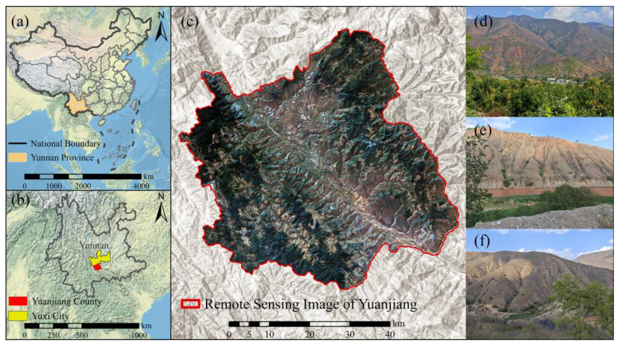
2.1. Study Area

Yuanjiang County is located in the south-central part of Yunnan Province (101°39′~102°22′E, 23°19′~23°55′N), with a total area of 2858 km2. The highest altitude in the region is 2580 m, the lowest altitude is 327 m, and the height difference is 2253 m. It has a typical deep-cut river valley landform, with the valley distributed in a narrow strip, surrounded by mountains, steep slopes, and closed terrain (Figure 1). The unique topographic features, including deep valleys and steep mountain slopes, enhance local climatic effects such as foehn winds and valley breezes, creating a persistently hot and dry climate within the valley. Yuanjiang belongs to the northern tropical semi-arid climate; the influence of the monsoons and topography generates pronounced spatial variations in rainfall, resulting in precipitation gradients that generally decrease from surrounding mountain ridges to valley bottoms. Specifically, due to the barrier effect of the Qinghai–Tibet Plateau and the Yunnan-Guizhou Plateau, the invasion of cold air in winter is prevented, while the Ailao Mountains in the west intercept the southwest warm and humid airflow from the Bay of Bengal. The significant Foehn effect makes the area one of the hottest and driest river valleys in China [24].
The climate in the region is distinctive, with sufficient heat but scarce water. The summer lasts for 9 months, with the climate characteristics of long summer without winter and continuous autumn and spring. The average annual temperature is 24.1 °C, and precipitation is mainly concentrated in the rainy season (May to October). The annual precipitation is less than 800 mm, the annual evaporation is as high as 2750 mm, and the dryness is 3.3. The annual active accumulated temperature of Yuanjiang, with a stable daily average temperature of ≥10 °C, is close to 9000 °C, and the daily average temperature throughout the year is greater than 10 °C [25]. It is the area with the highest annual active accumulated temperature and the longest duration in Yunnan, which is conducive to agricultural production and has become an important tropical fruit planting area in the country. The vegetation type is mainly drought-resistant and heat-resistant herbaceous plants. The landscape is similar to the African Tropical Savanna, and it is also known as the ‘Chinese Savanna’ [26]. Despite the rich light resources, the prominent human-land and water-heat contradictions in the dry and hot river valley make it one of the most fragile areas of China’s ecological environment, and land degradation and vegetation species loss are particularly serious [27].

2.2. Data Sources

2.2.1. Reference Land Use Datasets

For sample selection, three non-homogeneous commonly used publicly available land use/land cover products were employed: ESA World Cover 2020, Google Dynamic World 2020, and ESRI Land Cover 2020, all at 10 m spatial resolution. ESA World Cover is a global 10 m land cover product released in 2020 by the European Space Agency (ESA), with an overall accuracy of about 75% globally [11]. Google Dynamic World is a near real-time 10 m LULC product generated by Google and the World Resources Institute using deep learning, with a reported global overall accuracy of 73.8% [12]. ESRI Land Cover is a land use dataset produced by ESRI using artificial intelligence techniques, with a global overall accuracy of 85% [13]. To improve the reliability of these heterogeneous data sources as reference samples, we used the 2020 version for all three products to ensure temporal consistency.

2.2.2. Remote Sensing Imagery

All classified images used in this study were acquired through the Google Earth Engine (GEE) platform, including preprocessed Sentinel satellite images (2018~2023). The Sentinel satellite series was developed by the European Space Agency (ESA) under the Copernicus program to provide high-resolution earth observation data.
The multispectral data analysis uses the level-2A surface reflectance (SR) product (COPERNICUS/S2_SR_HARMONIZED), which has been orthorectified and atmospherically corrected. The product contains 13 spectral bands covering visible (VIS), near-infrared (NIR), and shortwave infrared (SWIR) wavelengths, ranging from 442.3 nm to 2202.4 nm. The spatial resolution of each band is 10 m, 20 m, and 60 m, respectively, and the revisit period of a single satellite is 10 days. Through the complementary operation of the two satellites, the combined revisit period is shortened to 5 days [28]. The Sentinel-2 dataset uses the quality detection band QA60 and the sentinel-2 cloud detector library to determine the S2 cloud probability, remove the clouds in the image, and then obtain the monthly scale image through median synthesis.
The synthetic aperture radar (SAR) data are collected in interferometric wide swath (IW) scanning mode as Sentinel-1 C-SAR Ground Range Detection (S1_GRD) products. This mode combines ascending and descending orbits and is processed using Doppler centroid estimation and single-look complex (SLC) focusing. The data are further processed using the Sentinel-1 toolbox to produce calibrated orthophoto products. Each scene contains four bands with a resolution of 10 m. Sentinel-1 provides four polarization modes: (1) single co-polarization VV (vertical transmit/vertical receive); (2) single co-polarization HH (horizontal transmit/horizontal receive); dual polarization modes: (3) VV+VH (vertical transmit/vertical receive and vertical transmit/horizontal receive) and (4) HH+HV (horizontal transmit/horizontal receive and horizontal transmit/vertical receive).
In addition, Chinese GaoFen series high-resolution satellite images were used to refine and validate samples further. We obtained 16 scenes from GaoFen-2 (GF-2) and 10 scenes from GaoFen-7 (GF-7) in 2024. GF-2 is China’s first sub-meter civilian optical remote sensing satellite; it carries two panchromatic cameras with 1 m resolution (and 4 m multispectral) that can image side-by-side, achieving a swath width of 45 km. GF-2 has a revisit period of no more than 5 days for any location worldwide. GF-7 is equipped with a dual-line array stereo mapping camera that can capture stereo panchromatic imagery at a resolution of better than 0.8 m (20 km swath) and multispectral imagery at 3.2 m resolution.

2.2.3. DEM Data

For topographic features, we used the Shuttle Radar Topography Mission (SRTM) digital elevation model at 30 m resolution, available via GEE. SRTM was a mission conducted by NASA and NGA in 2000 aboard the Space Shuttle Endeavor, which generated near-global elevation data using interferometric radar [29]. The SRTM DEM provides continuous elevation coverage and is widely used for terrain analysis.

2.3. Methods

2.3.1. High-Accuracy Sample Datasets Construction

The stratified random sampling method was mainly used in the process of constructing the sample set. Stratified sampling is also called type sampling. It first divides the population to be studied into different layers (groups) according to certain characteristics or rules and then independently and randomly selects individuals from each layer (group) in equal proportion or optimal proportion. Finally, the samples of each layer are combined to estimate the target quantity of the population. In land use classification, stratified random sampling is used to select a certain number of samples from different land type samples randomly. This sampling method ensures that the sample contains sampling units with various characteristics and that the sample structure is relatively close to the overall structure, which can effectively improve the accuracy of the estimate. To address class balance in the training data, the sample datasets were built in three main steps:
(1)
Classification Scheme Alignment and Initial Screening
We first unified the land use classification scheme to the target system (the “Land Use Classification Scheme for Field Survey Units of the National Soil Erosion Survey in China.” (Appendix A.1)). Using the three heterogeneous land cover datasets (ESA World Cover, Google Dynamic World, and ESRI Land Cover) as references, we reconciled their land class definitions to the target classification. Each product’s original classes were converted or merged into the target land use classes accordingly.
(2)
Non-homologous data voting
The concept of non-homologous data voting originates from pure pixels in image classification. The basic idea is to overlay the multiple land cover datasets spatially and identify areas where the different products agree on the land type. If a pixel’s classification is consistent across the three datasets (high agreement), we retain that label as a candidate reference sample. For pixels that are consistent in all products, the classification results are used as reference sample data for further classification.
(3)
Sample Refinement and Precision Correction
For minority land classes (such as orchard land, bare land, industrial/mining land, etc.), we supplemented and corrected samples using high-resolution imagery and field investigations. To reduce errors due to subjective differences in manual interpretation, multiple experts independently interpreted the high-resolution GF-2 and GF-7 images. Discrepancies among interpreters were resolved through discussion or additional field verification; if consensus could not be reached, those sample points were discarded. Unstable samples (e.g., seasonal water bodies) were also removed. Considering the local characteristics of the Yuanjiang dry–hot valley and the practical needs of soil conservation, we reclassified land use into eight primary categories: cultivated land (annual crops), garden plantations (perennial crops, e.g., orchards and plantations), woodland, grassland, residential and mining land, transportation land, water bodies, and other land types (such as bare soil, etc.). We ensured a minimum spacing of >10 m between sample points. An initial sample set was obtained through stratified random sampling across these categories. Finally, we compared classifications on different periods of image sets and selected only those pixels that remained consistently classified (pure and temporally stable) as the high-accuracy sample set.
Using this procedure, we initially obtained about 7900 sample points. After high-resolution visual interpretation and correction, we finalized high-accuracy sample datasets of 5918 points, distributed as follows: cultivated land 1198; garden plantations 857; woodland 1526; grassland 1254; residential and mining land 396; transportation land 200; water bodies 276; other land 211, as shown in Figure 2.

2.3.2. Imbalanced Sample Datasets Design

In this study, the imbalance ratio (IR) is employed to quantify the degree of class imbalance in a sample dataset. IR is defined as the ratio of the number of samples in the majority class to that in the minority class:
IR = N majority   class N minority   class
where  N majority   class  is the sample count of the majority class and  N minority   class  is that of the minority class.
According to the published authoritative results of the Third National Land Survey (2019) for the study area, cultivated land covered 223.00 km2 (7.80% of the county), garden plantations 298.68 km2 (10.45%), woodland 1887.82 km2 (66.05%), and grassland 93.74 km2 (3.28%). Clearly, woodland area far exceeds that of other land types. Thus, in our study, we designate forest land as the majority class and cultivated land, garden plantations, and grassland as minority classes of interest. We further constructed both a balanced dataset and several imbalanced datasets as follows:
(1)
Balanced dataset
From the high-accuracy sample database, we drew a stratified random sample of 200 points for each of the 8 land categories, yielding a balanced dataset (equal sample size per class). This balanced set was used for feature selection and for comparing classifier performance without class imbalance bias.
(2)
Unbalanced datasets
We created three groups (Group 1: Woodland vs. Cultivated land, Group 2: Woodland vs. Garden Plantations, Group 3: Woodland vs. Grassland) of imbalanced sample sets to specifically examine the effect of imbalance between woodland and each minority class.
In each group, we fixed the sample counts of all other land classes (the ones not involved in the pair) at 200 each and varied the sample counts of the target minority class and the woodland class to achieve a series of IR values. Specifically, for each group, we generated sample sets with IR values ranging from 1 to 15 (in integer steps). For example, in Group 1, the cultivated land vs. forest samples ranged from an even 1:1 ratio (both classes 800 samples, IR = 1) to an extreme 1:15 ratio (cultivated land 100 samples vs. forest 1500 samples, IR = 15), as detailed in Table 1. Similarly, Group 2 and Group 3 datasets were constructed by varying garden plantation land or grassland (respectively) against woodland over the same series of IR values. These imbalanced datasets allow us to analyze classification performance under progressively more imbalanced training conditions.

2.3.3. Classification Algorithms and Feature Selection on GEE

Google Earth Engine provides a cloud platform for geospatial analysis with massive remote sensing data, removing traditional barriers in data acquisition and preprocessing. Its powerful parallel computation and vast data catalog enable large-area, long time-series, and high spatio-temporal resolution remote sensing studies.
In this work, we chose traditional machine learning classifiers on the GEE platform to handle imbalanced data for land cover classification, instead of deep learning methods, for several reasons: (1) Traditional classifiers require less computational power and have lower training complexity; (2) They offer greater model interpretability, with clearly understandable feature importance, in contrast to the ‘black box’ nature and low transparency of deep learning models; (3) These models are easier to migrate and reuse within the GEE environment, making them more suitable for small datasets or those with limited features; (4) Class imbalance can be effectively mitigated through techniques such as adjusting sample weights, oversampling, whereas deep learning models typically require more extensive parameter tuning to avoid bias and overfitting.
Using the GEE platform, we integrated multi-dimensional features of spectral, textural, and topographic features as main inputs (summarized in Table 2) and evaluated four widely used machine learning classifiers for feature selection and classification performance evaluation:(1) Support vector machine (SVM), which is suitable for high-dimensional space and small sample data, has strong generalization ability and can solve nonlinear classification problems; (2) Classification and regression tree (CART), which uses a binary tree structure to recursively split features to achieve classification; (3) Gradient boosting tree (GTB), which constructs a decision tree through serial iteration to correct the prediction error of the previous tree; (4) Random Forest (RF), which integrates multiple decision trees and votes to improve the stability and generalization ability of the model [30].
To quantify each feature’s ability to discriminate land classes, we employed the coefficient of variation (CV), which measures the dispersion of a distribution as the ratio of the standard deviation to the mean. Here, CV is used to evaluate the separability of each feature across the 8 land classes: a higher CV (among classes) implies better discrimination ability for that feature. CV is defined as:
CV = σ μ
σ = i = 1 n X i μ 2 / n
μ = i = 1 n X i n
where μ is the mean and σ the standard deviation of a feature value across all samples of all classes (or across class means, depending on context). In practice, we compute CV for a feature across the set of class mean values to assess how much the feature varies between land use categories (the more it varies, the better it separates the classes).  X i  represents the value of each pixel, and  n  represents the number of pixels.

2.3.4. Accuracy Evaluation

For each classification experiment, the dataset was randomly split 50:50 into a training set and an independent validation set. Using the validation samples, we computed a confusion matrix and evaluated four accuracy metrics to assess classification performance: Overall Accuracy (OA), Producer’s Accuracy (PA), User’s Accuracy (UA), and the Kappa coefficient. These metrics are defined as follows:
PA =   n ii n * i × 100 %
UA = n ii n i * × 100 %
OA = i = 1 m n ii n × 100 %
Kappa = P 0 P e 1 P e   ( P 0 = OA ,   P e = i = 1 q n i * × n * i n 2 )
In the formula,  i  represents pixel;  n  represents the total number of pixels;  n ii  represents the pixel at the diagonal position of the confusion matrix;  m  represents the total number of diagonal pixels of the confusion matrix;  q  represents the number of categories in the confusion matrix;  n i *  represents the sum of row pixels of a certain category in the confusion matrix;  n * i  represents the sum of column pixels of a certain category in the confusion matrix.

3. Results

3.1. Feature Optimization and Time-Series Curve Analysis

After obtaining the classification results in GEE, a feature importance dictionary was automatically generated. Importance weights for a total of 59 features were extracted by inputting monthly synthetic remote-sensing images into the classifier. Based on the feature importance distribution shown in Figure 3, two feature optimization strategies were developed: (1) Removing insignificant features: A total of 22 redundant features—such as B6, B7, B8, B8A, MSAVI, CCRI, CI, DVI, EVI, GEMVI, GNDVI, NDCI, NDVI, RVI, TVI, VGCI, CIre, IRECI, R_TVI, gray_asm, gray_sent, and gray_ent—were removed, retaining 37 high-contribution features; (2) Retaining only significant features: 21 features with strong contributions to classification were selected, including B1, B2, B9, elevation, slope, aspect, hill shade, BSI, MNDWI, NDBI, SAVI, GI, MCRC, NDRI, NDSVI, NDTI, STI, RNDVI, SWIRVI, VH, and VV.
As illustrated in Figure 4, the efficiency of the classification model improved significantly following feature optimization. When the number of input features was reduced from the original 59 to 21, classification accuracy not only remained stable but actually improved to a certain extent. This outcome demonstrates that effective feature selection can eliminate redundant information, emphasize class distinctions, and enhance both the accuracy and precision of the classification model.
Considering the spectral synchronization and confusion between natural vegetation and crops in the dry–hot valley area, among the 21 preferred features, the greenness index (GI), normalized difference tillage index (NDTI), soil conditioned vegetation index (SAVI), and simple tillage index (STI) in the spectral features have a significant impact on the classification results. Spectral time series curves are established for them, respectively (Figure 5). These indices were chosen because they were identified as the most discriminative spectral features for separating the land classes. We extracted the monthly values of these four indices from 2017 through 2023 for each land use class and plotted their 7-year time series (Figure 5). The time-series curves exhibit pronounced seasonal periodicity for each land class, reflecting phenology or land use practice cycles. These distinctive temporal patterns help distinguish different land use types. For example, certain indices for cultivated land oscillate according to crop growing seasons, whereas woodland shows more stable trends. The clear periodic differences among classes suggest that incorporating multi-temporal data can aid classification.
To further analyze the temporal separability of classes, we calculated the coefficient of variation (CV) of these spectral features across the 8 land classes for each month and year. After removing outliers and normalizing, we obtained the mean CV of the four selected indices for each month of each year. A higher CV means the feature values vary more among land classes, indicating better class separability. The results (Figure 6) show that in years 2017, 2018, 2019, and 2022, the overall CV values were relatively low, implying that land classes were less distinguishable using these features in those years. In contrast, the years 2020, 2021, and 2023 exhibited higher CV values, meaning the spectral characteristics provided stronger discrimination between classes. Focusing on the intra-annual pattern, the period from February to April each year consistently showed higher CV values. This indicates that the spectral differences between land use types are most pronounced in late winter to early spring. In other words, February–April is the optimal time window for distinguishing land classes in the dry–hot valley, as vegetation and land cover differences are maximized during this period (likely due to phenology stages and minimal rainfall amounts). This finding is important for scheduling image acquisitions for classification in similar environments.

3.2. Accuracy Comparison of Different Classification Strategies

We compared the performance of four machine learning classifiers (SVM, CART, GTB, RF) for land use mapping under various temporal image compositing scenarios. For Gradient Tree Boosting (GTB) and Random Forest (RF), we optimized the number of decision trees (testing values from 1 to 50) to ensure the best performance for each case. Based on the CV analysis above, we selected representative time composite images as inputs. Figure 7 shows the classification accuracy comparison results of different machine learning algorithms combined with synthetic images of different time scales (single month, three months, half a year, and annual synthesis). Among them, the classification accuracy of annual scale synthetic images is significantly higher than that of single-month, three-month, three-year months, and year synthetic images, which shows that image synthesis with a longer time scale can more effectively capture the seasonal changes and characteristic differences in different land types and improve the classification and distinction ability.
Among the four classification algorithms, the ensemble methods (GTB and RF) generally outperformed SVM and CART, given sufficient tree numbers, indicating that the ensemble learning method based on decision trees is more suitable for handling regional remote sensing classification tasks such as dry–hot valleys with complex land distribution and strong heterogeneity. Specifically, the highest overall accuracy was achieved using the 2020 annual composite image classified with the Gradient Tree Boosting algorithm. This combination yielded the best performance in terms of OA and other metrics. Therefore, we selected the 2020 annual composite and the GTB classifier as the optimal classification scheme to use in the subsequent class imbalance analysis.

3.3. Impact of Class Imbalance on Classification Accuracy

3.3.1. Woodland vs. Cultivated Land Imbalance Experiment

In Experiment 1, we varied the ratio of woodland (majority) to cultivated land (minority) samples (Group 1 dataset) while keeping other classes constant. The results show that as the imbalance ratio IR increases (i.e., woodland samples increase, and cultivated land samples decrease):
(1)
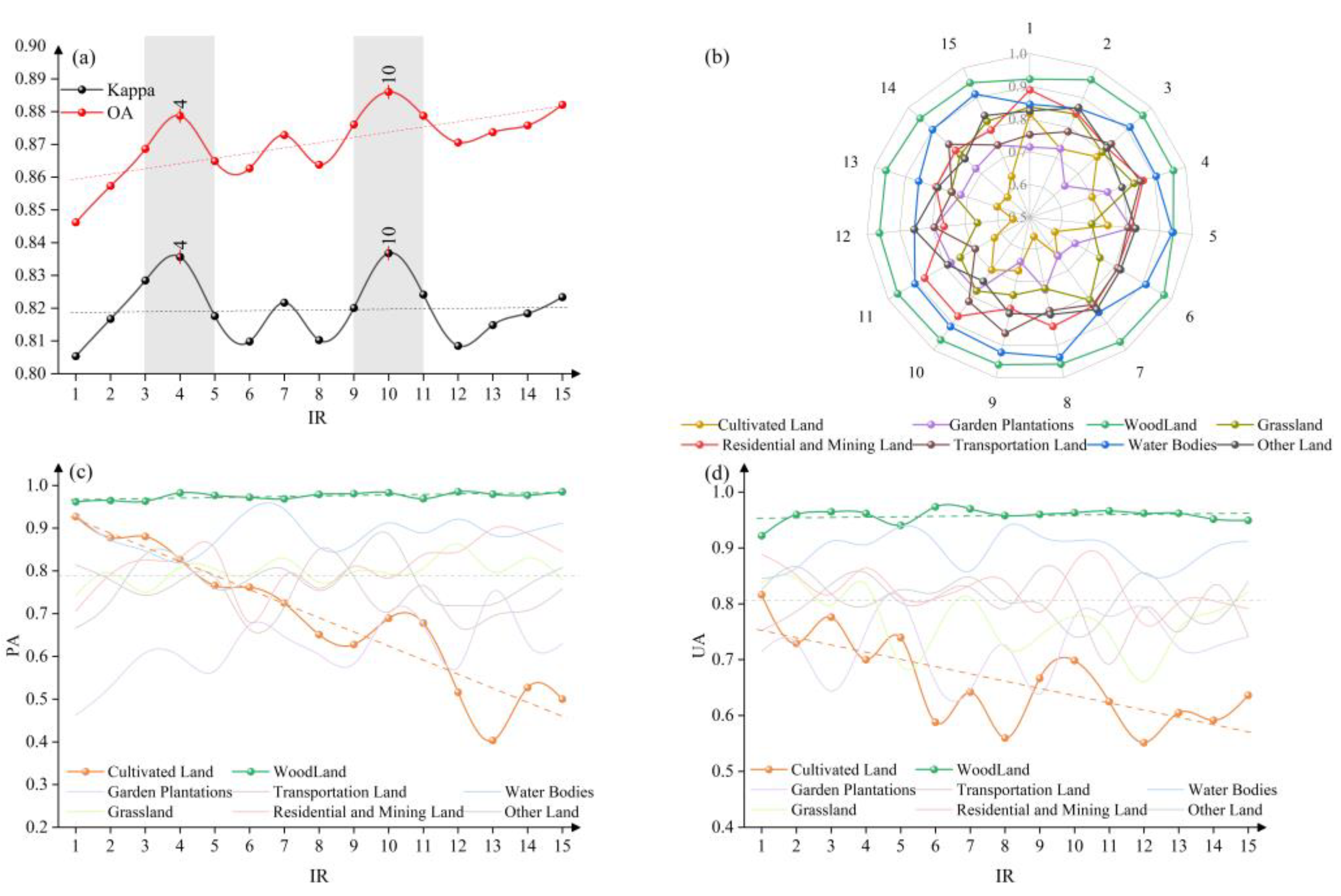
The OA of the classification increases monotonically. This suggests that reducing the proportion of the hard-to-classify minority class (cultivated land) in the training data can inflate the overall accuracy, likely because the classifier focuses on the easier majority class.
(2)
The Kappa coefficient fluctuated with increasing IR but did not exhibit a clear upward trend and did not increase as consistently as OA (Kappa accounts for agreement by chance and is more sensitive to imbalanced distributions). The highest OA and Kappa were achieved at an intermediate imbalance level of IR = 10, reaching 88.6% and 83.7%, respectively.
(3)
The PA and UA for cultivated land both decreased markedly as IR increased (i.e., as cultivated land had fewer training samples). Notably, at IR = 15 (the most imbalanced scenario), cultivated land’s PA dropped by 46%, and its UA dropped by 22% compared to the balanced case. This sharp decline indicates that cultivated land is highly susceptible to omission errors under class imbalance; many cultivated land samples were missed by the classifier when its training presence was small. Except for woodland and cultivated land, the classification accuracy of other land types fluctuated with the change in IR value but did not show obvious regularity (Figure 8).

3.3.2. Woodland vs. Garden Plantations Imbalance Experiment

In Experiment 2, we adjusted the ratio of forest to garden plantation samples (Group 2 dataset). The results indicate:
(1)
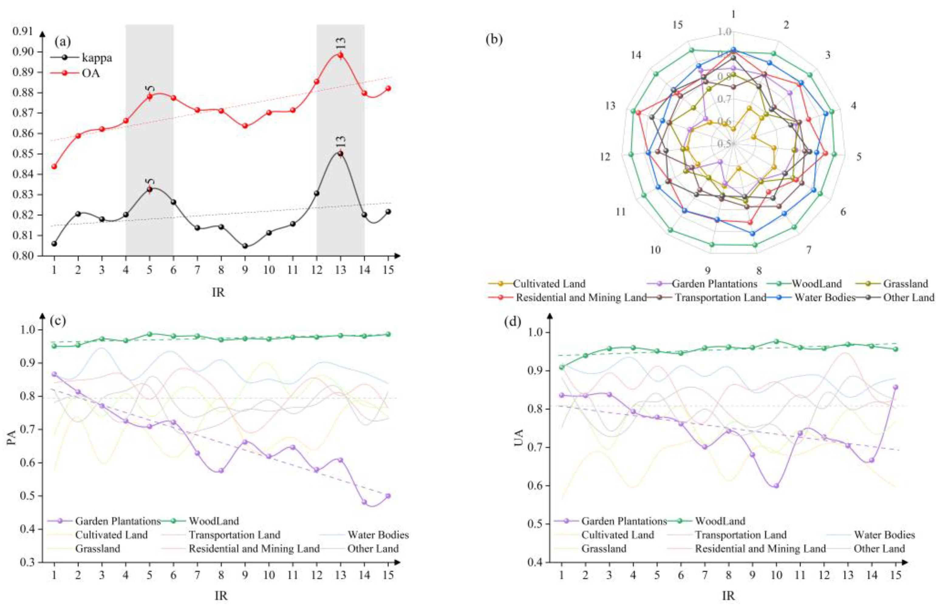
Both OA and Kappa increased as IR increased, with OA rising more steeply than Kappa. This again reflects that overall accuracy benefits from emphasizing the majority class (woodland), though the improvement in Kappa (which considers the full error matrix) is more tempered. At IR = 13, the OA and Kappa reached their maximum values of 89.8% and 85.1%, respectively.
(2)
The PA for garden plantations showed a clear downward trend as IR increased, indicating a growing omission error for under greater imbalance. The UA for garden plantations did not show a consistent trend; it fluctuated and was relatively unstable across IR levels. At IR = 15, garden plantations’ PA had decreased by 42%, whereas its UA paradoxically increased by about 2.5%. This suggests that at a very high imbalance, the classifier seldom predicts the minority class at all; those few predictions might be mostly correct (hence a slight UA rise), but many actual garden plantation areas are being misclassified as something else (hence a large PA drop). In effect, garden plantation samples were largely omitted from the classification when they became too scarce in training, demonstrating a severe impact of class imbalance.
(3)
By contrast, PA and UA of woodland were relatively stable, showing little effect from the changing IR. Aside from garden plantations and woodland, the other classes again showed some fluctuations in accuracy with changing IR but no strong systematic trends (Figure 9).

3.3.3. Woodland vs. Grassland Imbalance Experiment

In Experiment 3, we varied the ratio of woodland to grassland samples (Group 3 dataset). The observed patterns were:
(1)
Both overall accuracy and Kappa increased as IR increased, similar to the previous experiments. The OA rose more noticeably than Kappa. At IR = 13, we obtained the highest values (OA ≈ 90.0%, Kappa ≈ 85.0%).
(2)
Grassland’s PA and UA both declined as IR increased, indicating that grassland became harder for the classifier to correctly identify with fewer training samples. At IR = 15, the grassland’s PA had fallen by about 25% and its UA by about 18% compared to the balanced scenario. This decline, although significant, was less drastic than what we saw for cultivated land and garden plantations, suggesting grassland is less sensitive to imbalance.
(3)
Woodland again achieved the highest class-specific accuracy; the PA and UA remained largely unaffected by the imbalance level, reinforcing that the majority class did not suffer from the imbalance increase (Figure 10).
After conducting all three imbalance experiments, we compared the outcomes for the three minority classes (cultivated land, garden plantations, and grassland). Overall, as the imbalance ratio IR increased (i.e., as the proportion of majority class samples grew relative to the minority class), the OA of the classification consistently showed an upward trend. This is expected since the classifier performance metric is dominated by the well-represented majority class. However, the classification accuracy of the minority classes declined significantly with increasing IR. Among the three tested minority types, cultivated land was the most adversely affected by class imbalance, followed by garden plantations, and then grassland showed the least severe decline (though still notable). For example, cultivated land experienced the largest drop in PA under high imbalance, indicating it is most prone to being omitted. PA of garden plantations also dropped substantially, while its UA varied irregularly, reflecting considerable omission errors and some inconsistency in commission errors. Grassland showed a smaller decrease in accuracy metrics relative to the others, suggesting slightly better resilience but still a clear negative effect. In contrast, woodland (the majority class) maintained stable accuracy across different IR values, affirming that the majority class’s performance is largely insensitive to the imbalance.
It is important to note that although the accuracy of minority classes plummets with higher IR, overall accuracy can increase misleadingly. This means that in class-imbalanced scenarios, the model may appear to perform better in aggregate while actually performing worse on the critical minority classes (which, in this context, are often the land types most relevant for soil erosion risk). Additionally, aside from the majority and minority classes in question, the accuracy of other land categories showed noticeable variability as IR changed, though without a consistent directional pattern. This indicates that class imbalance can indirectly introduce noise in the classification of other classes as well, perhaps due to shifts in decision boundaries as the classifier is biased toward the majority class. In summary, class imbalance had differing levels of impact on each land use class. Cultivated land suffered the greatest accuracy loss under imbalanced training, garden plantations also showed severe accuracy reduction (especially in PA), and grassland had a significant but comparatively smaller decline. Meanwhile, forest land and water bodies (which were abundant or easier to classify) retained relatively high accuracy even in imbalanced scenarios, and classes like built-up land and others exhibited fluctuations. The greater vulnerability of cultivated land and garden plantations to omission errors under imbalance is likely related to their inherent spectral-temporal characteristics and confusion with other classes, whereas woodland’s distinctive features made it robust as the majority class.

4. Discussion

The Yuanjiang dry–hot valley region is characterized by complex terrain and diverse land types, posing significant challenges for refined land use classification. Relying on data from a single sensor is insufficient to meet the accuracy requirements. Although the fusion of multi-source remote sensing data has partially addressed this limitation, it also introduces new challenges, such as scale effects during sample selection and feature extraction, which in turn increase the uncertainty of classification results. From a spatial scale perspective, low-resolution data are often incapable of capturing fine-grained texture information, which can result in the misclassification or mixing of different land types, thereby reducing overall classification accuracy [31]. From a temporal scale perspective, surface changes and climatic variability hinder the acquisition of stable samples with consistent spatio-temporal characteristics [32].
This study comprehensively integrates three publicly available land use products, ESA World Cover, Google Dynamic World, and ESRI Land Cover, along with Sentinel series data with a spatial resolution of 10 m and high-resolution satellite imagery with resolutions finer than 1 m. Although feature optimization, image time series synthesis, and the selection of appropriate classifiers can effectively enhance classification accuracy [33], the problem of class imbalance continues to be a major constraint, especially in the accurate classification of minority land use classes. Under imbalanced conditions, even if overall classification accuracy improves, the accuracy for minority classes, such as cultivated land, garden plantations, and grassland, is often significantly reduced. This can adversely affect the accurate identification and assessment of regional soil erosion risks. Since these minority classes are typically erosion-prone types, classification errors or omissions may lead to underestimation of erosion risks, ultimately undermining the scientific validity and effectiveness of soil and water conservation measures as well as ecological restoration efforts. Therefore, improving the classification accuracy of these sensitive land categories is critical for enhancing the precision of soil erosion prediction and risk assessment.
Future research should prioritize the development of long-term, stable, and transferable sample sets, as well as the further optimization of multi-scale feature fusion methods. Sample optimization techniques such as the SMOTE algorithm, which generates new minority class samples by interpolating existing ones to balance the dataset; the ADASYN algorithm, which adaptively assigns weights based on the learning difficulty of minority samples to create more representative synthetic data; and cost-sensitive learning approaches, which assign different penalties to different types of misclassifications, and significantly enhance the granularity and accuracy of land use classification. These improvements are essential for meeting the demands of real-world applications [34].
Although remote sensing technology has been widely applied in soil erosion studies, the accurate acquisition of detailed land use information at regional scales remains a significant challenge. Overcoming this limitation requires not only the use of higher-resolution remote sensing data and the refinement of classification algorithms to address class imbalance but also the integration of environmental variables, such as rainfall, topography, and soil properties, to enhance understanding of the spatial distribution patterns of critical land use types. Moreover, improving model adaptability to complex terrain is essential for more accurately identifying high erosion risk areas, such as bare land and steep slope farmland. These advancements will contribute to the development of more precise soil erosion risk assessment models, provide a stronger scientific basis for soil conservation efforts, and support the integration of erosion control with ecological protection objectives. Ultimately, this will facilitate the coordination of conservation planning and ecological restoration, promoting sustainable land management in dry–hot valley regions.

5. Conclusions

To address the practical needs of soil and water conservation research in dry–hot valleys, this study integrated multi-source remote sensing data with high-resolution visual image interpretation to construct a high-precision, stable sample set. Various machine learning methods and classification strategies were then applied to thoroughly analyze the problem of class imbalance in land use classification and its impact on classification accuracy. The main conclusions are as follows:
(1)
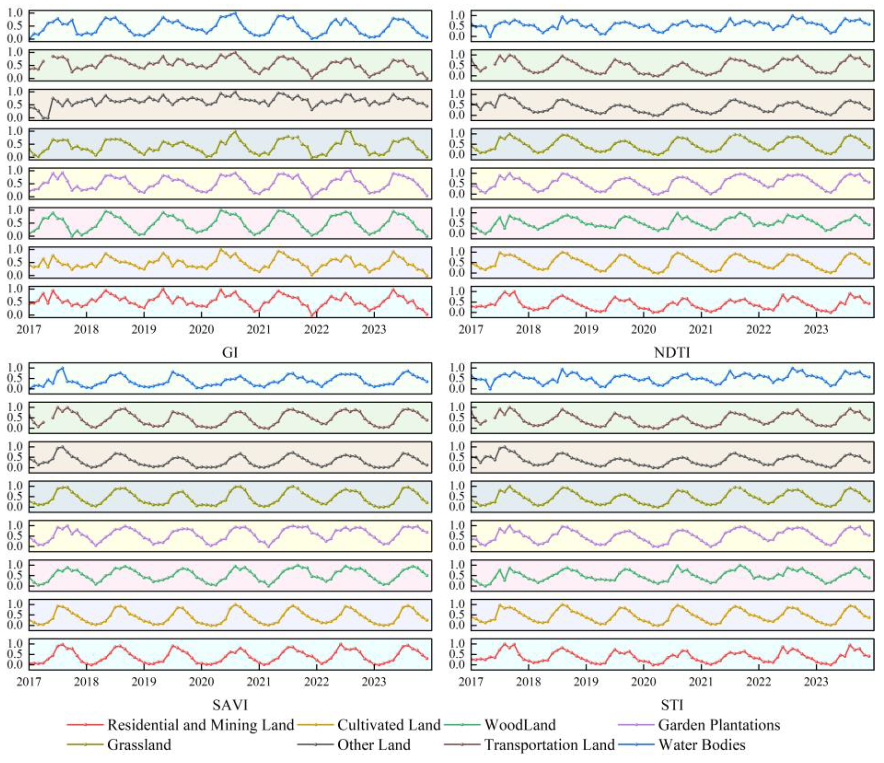
Through feature optimization, the number of features was reduced from 59 to 21, leading to improvements in both classification efficiency and accuracy. Among these, GI, SAVI, NDTI, and STI were identified as the most discriminative spectral features. Based on these four indicators, monthly spectral time series curves from 2017 to 2023 were constructed, and the coefficient of variation (CV) between land use classes was calculated. The results indicated that the spectral features exhibited the greatest discriminative ability between February and April each year, identifying this period as the optimal time window for land use classification in dry–hot valleys.
(2)
Based on spectral time series analysis, synthetic images were generated at different temporal scales—single-month, three-month, half-year, and annual. These were used as inputs to four machine-learning algorithms for classification comparison. The results showed that the combination of annual-scale synthetic images from 2020 and the Gradient Boosted Trees classifier yielded the highest classification accuracy, demonstrating that longer temporal integration can significantly enhance classification performance.
(3)
The class imbalance experiments revealed that as the imbalance ratio (IR) increased, both OA and the Kappa coefficient exhibited an upward trend. Interestingly, the highest OA and Kappa values in each experiment group occurred under the most imbalanced conditions. Among the land classes, the PA and UA for woodland were relatively stable and less affected by class imbalance. In contrast, the PA and UA of minority classes, such as cultivated land, garden plantations, and grassland, declined significantly, with PA showing a steeper drop. This suggests that under imbalanced conditions, minority classes are more prone to omission or misclassification.

Author Contributions

Conceptualization, methodology, funding acquisition, G.C.; data curation, software, writing—original draft preparation, formal analysis, Y.D.; resources, B.T.; data collection, review and editing, X.D.; validation, visualization, L.Z.; date processing, investigation, visualization, H.Z. All authors have read and agreed to the published version of the manuscript.

Funding

This research was supported by Yunnan Fundamental Research Projects (Grant Nos. 202401AT070366, 202501AT070326) and the National Natural Science Foundation Youth Project (Grant No. 42407096).

Data Availability Statement

Data are available upon request.

Acknowledgments

We would like to thank the Plateau Remote Sensing Innovation Research Team at Kunming University of Science and Technology for their valuable platform support.

Conflicts of Interest

The authors declare no conflicts of interest.

Appendix A

Appendix A.1

This appendix is the “Land Use Classification Scheme for Field Survey Units of the National Soil Erosion Survey in China”.
Table A1. Land Use Classification Scheme for Field Survey Units of the National Soil Erosion Survey in China.
Code1st-Level ClassCode2nd-Level ClassDetailed Descriptions
1Cultivated Land11Paddy FieldLand used primarily for growing aquatic crops such as rice and lotus, including areas practicing rotation between aquatic and dry crops.
12Irrigated LandLand with guaranteed water sources and irrigation facilities, generally irrigable under normal weather conditions for dry crops, including non-industrial greenhouse land for vegetables.
13Dry LandLand without irrigation facilities, mainly dependent on natural rainfall for dry crop cultivation, including land irrigated only by flood deposits.
2Garden Plantations21OrchardLand dedicated to the cultivation of fruit trees.
22Tea PlantationLand dedicated to the cultivation of tea plants.
23Other PlantationsLand cultivating perennial crops such as mulberry, rubber, cocoa, coffee, oil palm, pepper, medicinal plants, etc.
3Woodland31Forest LandWoodland with tree canopy coverage ≥ 20%, including mangroves and bamboo forests.
32ShrublandLand covered primarily with shrubs having a coverage ≥ 40%.
33Other Forest LandIncludes sparse forests (canopy coverage between 10% and 20%), unformed forests, cutover areas, nurseries, etc.
4Grassland41Natural GrasslandNatural grassland primarily used for grazing or haymaking.
42Artificial GrasslandGrassland planted with cultivated grasses.
43Other GrasslandLand with tree canopy coverage <10%, primarily soil-covered and grassy, not utilized for animal husbandry.
5Residential and Mining Land51Urban Residential AreaLand within urban areas designated for residential housing and associated facilities, including ordinary residences, apartments, and villas.
52Rural Residential AreaLand designated for residential housing in rural areas.
53Independent Industrial and Mining LandLand used primarily for industrial production and material storage.
54Commercial, Service, and Public Facilities LandLand mainly used for commercial services, institutional groups, publishing, education, science, culture, health, scenic spots, and public facilities.
55Special Purpose LandLand used for military facilities, foreign affairs, religious purposes, correctional facilities, cemeteries, etc.
6Transportation Land Land designated for transportation infrastructure, including airports, ports, docks, pipelines, and roads.
7Water Bodies Land comprising river surfaces, lakes, reservoirs, ponds, coastal tidal flats, inland flats, ditches, hydraulic structures, glaciers, and permanent snow, excluding flood detention areas and reclaimed flats used for farmland, orchards, forests, settlements, and roads.
8Other Land Includes lands not categorized above, such as saline-alkali land, marshland, sandy land, and bare land.

References

  1. Wuepper, D.; Borrelli, P.; Finger, R. Countries and the global rate of soil erosion. Nat. Sustain. 2020, 3, 51–55. [Google Scholar] [CrossRef]
  2. Liu, B.Y.; Yang, Y.; Lu, S.J. Discriminations on common soil erosion terms and their implications for soil and water conservation. Chin. J. Soil Water Conserv. 2018, 16, 9–16. (In Chinese) [Google Scholar]
  3. Montgomery, D.R. Soil erosion and agricultural sustainability. Proc. Natl. Acad. Sci. USA 2007, 104, 13268–13272. [Google Scholar] [CrossRef]
  4. Morgan, R.P.C. Soil Erosion and Conservation; John Wiley & Sons: Hoboken, NJ, USA, 2009. [Google Scholar]
  5. Wang, Z.; Hoffmann, T.; Six, J. Human-induced erosion has offset one-third of carbon emissions from land cover change. Nat. Clim. Change 2017, 7, 345–349. [Google Scholar] [CrossRef]
  6. Alewell, C.; Ringeval, B.; Ballabio, C.; Robinson, D.A.; Panagos, P.; Borrelli, P. Global phosphorus shortage will be aggravated by soil erosion. Nat. Commun. 2020, 11, 4546. [Google Scholar] [CrossRef] [PubMed]
  7. Pimentel, D.; Burgess, M. Soil erosion threatens food production. Agriculture 2013, 3, 443–463. [Google Scholar] [CrossRef]
  8. Borrelli, P.; Robinson, D.A.; Fleischer, L.R.; Lugato, E.; Ballabio, C.; Alewell, C.; Panagos, P. An assessment of the global impact of 21st century land use change on soil erosion. Nat. Commun. 2017, 8, 2013. [Google Scholar] [CrossRef]
  9. Borrelli, P.; Robinson, D.A.; Panagos, P.; Lugato, E.; Yang, J.E.; Alewell, C.; Ballabio, C. Land use and climate change impacts on global soil erosion by water (2015–2070). Proc. Natl. Acad. Sci. USA 2020, 117, 21994–22001. [Google Scholar] [CrossRef]
  10. Fofang, S.T.; Mukama, E.B.; Adem, A.A.; Dondeyne, S. Landcover Change Amidst Climate Change in the Lake Tana Basin (Ethiopia): Insights from 37 Years of Earth Observation on Landcover–Rainfall Interactions. Remote Sens. 2025, 17, 747. [Google Scholar] [CrossRef]
  11. Venter, Z.S.; Barton, D.N.; Chakraborty, T.; Simensen, T.; Singh, G. Global 10 m Land Use Land Cover Datasets: A Comparison of Dynamic World, World Cover and Esri Land Cover. Remote Sens. 2022, 14, 4101. [Google Scholar] [CrossRef]
  12. Brown, C.F.; Brumby, S.P.; Guzder-Williams, B.; Birch, T.; Hyde, S.B.; Mazzariello, J.; Tait, A.M. Dynamic World, Near real-time global 10 m land use land cover mapping. Sci. Data 2022, 9, 251. [Google Scholar] [CrossRef]
  13. Karra, K.; Kontgis, C.; Statman-Weil, Z.; Mazzariello, J.C.; Mathis, M.; Brumby, S.P. Global land use/land cover with Sentinel 2 and deep learning. In Proceedings of the 2021 IEEE International Geoscience and Remote Sensing Symposium IGARSS, Brussels, Belgium, 11–16 July 2021; IEEE: Piscataway, NJ, USA, 2021; pp. 4704–4707. [Google Scholar]
  14. Tsendbazar, N.; Herold, M.; Li, L.; Tarko, A.; De Bruin, S.; Masiliunas, D.; Duerauer, M. Towards operational validation of annual global land cover maps. Remote Sens. Environ. 2021, 266, 112686. [Google Scholar] [CrossRef]
  15. Khan, M.; Chen, R. Assessing the Impact of Land Use and Land Cover Change on Environmental Parameters in Khyber Pakhtunkhwa, Pakistan: A Comprehensive Study and Future Projections. Remote Sens. 2025, 17, 170. [Google Scholar] [CrossRef]
  16. Chen, G.; Zhao, J.; Duan, X.; Tang, B.; Zuo, L.; Wang, X.; Guo, Q. Spatial quantification of cropland soil erosion dynamics in the yunnan plateau based on sampling survey and multi-source LUCC data. Remote Sens. 2024, 16, 977. [Google Scholar] [CrossRef]
  17. Tong, Y.; Feng, W.; Song, Y.; Quan, Y.; Huang, W.; Gao, L.; Xing, M. Dynamic ensemble algorithm of SMOTE and rotation WoodLand for imbalanced hyperspectral remote sensing classification. J. Remote Sens. 2022, 26, 2369–2381. (In Chinese) [Google Scholar]
  18. Xu, L.L.; Chi, D.X. Machine learning classification strategy for imbalanced datasets. Comput. Eng. Appl. 2020, 56, 12–27. (In Chinese) [Google Scholar]
  19. Bi, J.; Zhang, C. An empirical comparison on state-of-the-art multi-class imbalance learning algorithms and a new diversified ensemble learning scheme. Knowl.-Based Syst. 2018, 158, 81–93. [Google Scholar] [CrossRef]
  20. Mellor, A.; Boukir, S.; Haywood, A.; Jones, S. Exploring issues of training data imbalance and mislabelling on random WoodLand performance for large area land cover classification using the ensemble margin. ISPRS J. Photogramm. Remote Sens. 2015, 105, 155–168. [Google Scholar] [CrossRef]
  21. Ebrahimy, H.; Wang, Y.; Zhang, Z. Utilization of synthetic minority oversampling technique for improving potato yield prediction using remote sensing data and machine learning algorithms with small sample size of yield data. ISPRS J. Photogramm. Remote Sens. 2023, 201, 12–25. [Google Scholar] [CrossRef]
  22. Xiao, Y.; Huang, J.; Weng, W.; Huang, R.; Shao, Q.; Zhou, C.; Li, S. Class imbalance: A crucial factor affecting the performance of tea plantations mapping by machine learning. Int. J. Appl. Earth Obs. Geoinf. 2024, 129, 103849. [Google Scholar] [CrossRef]
  23. Liu, B.; Duan, X.; Wang, N.; Gu, Z.; Du, P. Sources of sediments during rainfall in the dry-hot valley region of China on a small watershed scale. J. Soil Water Conserv. 2021, 76, 14–24. [Google Scholar] [CrossRef]
  24. Palazzi, F.; Biddoccu, M.; Borgogno Mondino, E.C.; Cavallo, E. Use of Remotely Sensed Data for the Evaluation of Inter-Row Cover Intensity in Vineyards. Remote Sens. 2023, 15, 41. [Google Scholar] [CrossRef]
  25. Liu, Y.; Xie, M.; Qin, C. Climate characteristics and genesis of savannah in the dry hot valley of Yuanjiang, Yunnan. Yunnan Geogr. Environ. Res. 2023, 35, 61–69. (In Chinese) [Google Scholar]
  26. Zhu, H.; Tan, Y.; Yang, Y. Review on savanna vegetation in the dry hot river valleys of southwestern China. J. Plant Sci. 2024, 42, 682–696. (In Chinese) [Google Scholar]
  27. Yang, J.; Zhang, Z.; Shen, Z.; Ou, X.; Geng, Y.; Yang, M. Review of research on the vegetation and environment of dry-hot valleys in Yunnan. Biodivers. Sci. 2016, 24, 462. [Google Scholar] [CrossRef]
  28. Drusch, M.; Del Bello, U.; Carlier, S.; Colin, O.; Fernandez, V.; Gascon, F.; Bargellini, P. Sentinel-2: ESA’s optical high-resolution mission for GMES operational services. Remote Sens. Environ. 2012, 120, 25–36. [Google Scholar] [CrossRef]
  29. Yang, L.; Meng, X.; Zhang, X. SRTM DEM and its application advances. Int. J. Remote Sens. 2011, 32, 3875–3896. [Google Scholar] [CrossRef]
  30. Gorelick, N.; Hancher, M.; Dixon, M.; Ilyushchenko, S.; Thau, D.; Moore, R. Google Earth Engine: Planetary-scale geospatial analysis for everyone. Remote Sens. Environ. 2017, 202, 18–27. [Google Scholar] [CrossRef]
  31. Zhang, Y.; Fang, L.; Qiao, Z.; Chen, L.; Zhang, W.; Zheng, X.; Jiang, T. Remote sensing-based identification of WoodLand types and the scale effect in subtropical evergreen WoodLands. Chin. J. Ecol. 2020, 39, 1636. (In Chinese) [Google Scholar]
  32. Huang, H.; Wang, J.; Liu, C.; Liang, L.; Li, C.; Gong, P. The migration of training samples towards dynamic global land cover mapping. ISPRS J. Photogramm. Remote Sens. 2020, 161, 27–36. [Google Scholar] [CrossRef]
  33. Chen, B.; Huang, B.; Xu, B. Multi-source remotely sensed data fusion for improving land cover classification. ISPRS J. Photogramm. Remote Sens. 2017, 124, 27–39. [Google Scholar] [CrossRef]
  34. Gong, P. Intelligent mapping with remote sensing, iMap. J. Remote Sens. 2021, 25, 527–529. (In Chinese) [Google Scholar] [CrossRef]
Figure 1. Maps of the study area showing (a,b) geographical location, (c) remote sensing imagery, and (df) typical landscapes.
Remotesensing 17 01628 g001
Figure 2. Spatial distribution of high-precision samples in the study area.
Remotesensing 17 01628 g002
Figure 3. Statistical boxplot map of the importance scores for 59 features.
Remotesensing 17 01628 g003
Figure 4. Accuracy comparison map of 24 monthly composite images using different feature sets, showing the improvement with feature optimization.
Remotesensing 17 01628 g004
Figure 5. Monthly time series curves of four main spectral characteristics from 2017 to 2023.
Remotesensing 17 01628 g005
Figure 6. Time series of the coefficient of variation (CV) of the four key spectral features among the eight land use types from 2017 to 2023.
Remotesensing 17 01628 g006
Figure 7. Classification result comparison for the four classifiers (SVM, CART, GTB, RF) under different temporal composite inputs (single-month, 3-month, half-year, annual).
Remotesensing 17 01628 g007
Figure 8. Results of imbalance Experiment 1 (woodland vs. cultivated land): trends of accuracy metrics with increasing IR. (a) Kappa and overall accuracy; (b) radar chart of UA; (c) PA; (d) UA.
Remotesensing 17 01628 g008
Figure 9. Results of imbalance Experiment 2 (woodland vs. garden plantations): trends of accuracy metrics with increasing IR. (a) Kappa and overall accuracy; (b) radar chart of UA; (c) PA; (d) UA.
Remotesensing 17 01628 g009
Figure 10. Results of imbalance Experiment 3 (woodland vs. grassland): accuracy metrics as a function of IR. (a) Kappa and overall accuracy; (b) radar chart of UA; (c) PA; (d) UA.
Remotesensing 17 01628 g010
Table 1. Sample sizes for three groups of imbalanced datasets (row 1 represents IR, row 2 represents minority class, and row 3 represents majority class).
IR123456789101112131415
Minority class800534400320267229200178160145133123114107100
Majority class80010671200128013331371140014221440145514671477148614931500
Table 2. Multi-dimensional features input features for classification.
No.Spectral CharacteristicsAbbreviationNo.Spectral CharacteristicsAbbreviation
1Bare Soil IndexBSI24Red-Edge Near-Infrared Normalized Difference Vegetation IndexREDNDVI
2Chlorophyll Absorption Reflectance IndexCARI25Red Edge Position IndexREP
3Chlorophyll Concentration Reflectance IndexCCRI26Red-Edge Normalized Difference Vegetation IndexRNDVI
4Chlorophyll IndexCigreen27Band Ratio Vegetation IndexRVI
5Red Edge Chlorophyll IndexCire28Soil Adjusted Vegetation IndexSAVI
6Difference Vegetation IndexDVI29Simple Tillage IndexSTI
7Enhanced Vegetation IndexEVI30Shortwave Infrared Vegetation IndexSWIRVI
8Global Environment Monitoring Vegetation IndexGEMVI31Triangular Vegetation IndexTVI
9Greenness IndexGI32Vegetation Growth Cycle IndexVGCI
10Green Normalized Difference Vegetation IndexGNDVI33Angular Second MomentAsm
11Inverted Red Edge Chlorophyll IndexIRECI34ContrastContrast
12Modified Crop Residue CoverMCRC35AutocorrelationCorrelation
13Improved Normalized Difference Water Bodies IndexMNDWI36VarianceVar
14Improved Soil Adjusted Vegetation IndexMSAVI37Inverse Difference MomentIdm
15Normalized Difference Building IndexNDBI38Sum Of AveragesSavg
16Normalized Difference Chlorophyll IndexNDCI39Sum Of VariancesSvar
17Normalized Difference Residue IndexNDRI40Sum Of EntropySent
18Normalized Difference Senescent Vegetation Index,NDSVI41EntropyEntropy
19Normalized Difference Tillage IndexNDTI42Slope AspectAspect
20Normalized Difference Vegetation IndexNDVI43SlopeSlope
21Normalized Difference Vegetation Index(B8A)NDVI8A44ElevationElevation
22Normalized Difference Water Bodies IndexNDWI45HillshadeHillshade
23Red Edge Triangular Vegetation IndexR–TVI
Disclaimer/Publisher’s Note: The statements, opinions and data contained in all publications are solely those of the individual author(s) and contributor(s) and not of MDPI and/or the editor(s). MDPI and/or the editor(s) disclaim responsibility for any injury to people or property resulting from any ideas, methods, instructions or products referred to in the content.

