One-Dimensional Convolutional Neural Network for Automated Kimchi Cabbage Downy Mildew Detection Using Aerial Hyperspectral Images

Abstract

Downy mildew poses a significant threat to kimchi cabbage, a vital agricultural product in Korea, adversely affecting its yield and quality. Traditional disease detection methods based on visual inspection are labor intensive and time consuming. This study proposes a non-destructive, field-scale disease detection approach using unmanned aerial vehicle (UAV)-based hyperspectral imaging. Hyperspectral images of the kimchi cabbage field were preprocessed, segmented at the pixel level, and classified into four categories: background, healthy, early-stage disease, and late-stage disease. Spectral analysis of the late and early stages of downy mildew infection revealed notable differences in the red-edge band, with infected plants exhibiting increased red-edge reflectance. To automate disease detection, various machine learning models, including Random Forest (RF), 1D Convolutional Neural Network (1D-CNN), 1D Residual Network (1D-ResNet), and 1D Inception Network (1D-InceptionNet), were developed. These models were trained based on a 0.2 sampling dataset, achieving overall accuracy scores of 0.907, 0.901, 0.909, and 0.914, along with F1 scores of 0.876, 0.845, 0.897, and 0.899, respectively. Overall, the results of this study revealed that the red-edge band reliably signaled the presence of downy mildew, and the 1D-InceptionNet model demonstrated the most effective performance for automatic disease detection.

1. Introduction

The kimchi cabbage (Brassica rapa pekinensis), a crucial leafy vegetable in Korea, is highly vulnerable to several plant diseases, notably downy mildew, black rot, and soft rot. Among these, downy mildew—caused by Hyaloperonospora brassicae—poses a particularly severe threat, capable of infecting the plant throughout its life cycle [1]. Thriving in cool weather conditions, downy mildew symptoms become noticeable during the spring and autumn seasons. The disease manifests as necrotic tissues on both the adaxial and abaxial surfaces of the leaves. Pale yellow spots gradually expand, accompanied by the development of a grayish-white moldy growth on the abaxial side as the disease progresses [2]. The increased humidity due to precipitation during these seasons further stimulates downy mildew growth. The rapid growth of downy mildew necessitates timely treatment to minimize plant damage. Disease identification based on visual observation represents one of the most fundamental methods in practice. However, this approach is time consuming, labor intensive, and subjective, requiring trained personnel for accurate assessment [3]. Moreover, diseases that are asymptomatic or not yet visible to the human eye cannot be detected through visual inspection.

Rapid, accurate, and stable performance in disease detection instruments can enhance the overall plant disease management system. Imaging techniques employing digital cameras, multispectral cameras, or hyperspectral cameras offer potential solutions to address this challenge [4]. Hyperspectral imaging (HSI) is a technique that captures the spectrum of an observed object and organizes it into arrays [5]. HSI produces a three-dimensional (3D) hyperspectral cube, with height and width as spatial dimensions and depth as the spectral dimension [6]. Compared to digital RGB or multispectral cameras, hyperspectral cameras offer advantages in identifying and discriminating target objects. Hyperspectral sensors provide detailed spectral information with a narrow band resolution, making them more sensitive to subtle changes in spectrum reflectance. This sensitivity allows them to detect the subtle chemical changes caused by disease infection in plants [7,8]. Modern agriculture relies on monitoring the crop status, which involves measuring plant health, nutrient supply, pesticide effects, and crop yield [9]. These objectives are typically achieved through sensor measurements and the implementation of decision support systems. In extensive and open fields, sensing devices often depend on unmanned aerial vehicles (UAVs) to conduct field surveys and collect essential field information. In recent years, UAVs have become more reliable and adaptable to varying payloads. Furthermore, hyperspectral cameras are now manufactured in more compact forms, enabling the integration of these two systems to create a non-destructive, field-scale disease detection system. However, the high cost of advanced sensors, particularly hyperspectral cameras, remains a significant barrier to their widespread adoption in practical agricultural applications.

HSI technologies can be utilized to measure and monitor the leaf reflectance for assessing the plant conditions. The reflectance of a plant can represent its chemical compounds and morphological features [10]. In leafy crops, plant health is primarily indicated by the leaf’s status, including its pigment composition, leaf structure, and water content. This status is reflected in the spectral characteristics and can be used to determine whether a plant is healthy or diseased. In a healthy plant, chlorophyll strongly absorbs blue and red light while reflecting relatively high proportions of green and infrared light. Often, the leaf chlorophyll content decreases when plants are affected by environmental stressors. Consequently, the absorption of visible light decreases, the reflectance increases, and a general yellowing of the leaves may be observed [11]. However, the latent disease symptoms within leaf tissues, such as mesophyll abnormalities, exhibit a high correlation with reflectance changes in the near-infrared (NIR) range (700–1400 nm). Previous studies have demonstrated that plant–pathogen interactions can alter the reflectance patterns at specific wavelengths. For example, Fernández et al. [12] found that powdery mildew-infected cucumber leaves showed increased reflectance at 520–530 nm and decreased reflectance at 400–450 nm. Song et al. [13] identified the key wavelengths (e.g., 970, 982, 1180 nm) effective for detecting rot disease in napa cabbage using hyperspectral imaging. Guo et al. [14] and Ma et al. [15] applied UAV-based hyperspectral technologies to detect wheat diseases, achieving R² values up to 0.88 using machine learning models.

Machine learning (ML) encompasses a wide range of algorithms capable of identifying the patterns and trends within datasets, which can then be used to make predictions on new data [16]. In agriculture, ML algorithms are primarily applied to automate the prediction of the crop status and yield, as well as to detect plant diseases [17]. Among these algorithms, Convolutional Neural Networks (CNNs) have demonstrated exceptional success in image-based tasks, owing to their ability to automatically extract both low- and high-level features, often outperforming traditional ML methods. For instance, Agarwal et al. [18] developed a 2D CNN with a modified activation function to classify the disease types and severity in cucumber plants, achieving an accuracy of 93.75%. Latif et al. [19] applied a deep CNN with transfer learning to identify six types of rice leaf disease, reaching an average accuracy of 96.08%. Similarly, Fang et al. [20] proposed a lightweight multiscale CNN that integrates residual and inception modules, yielding 98.7% accuracy in wheat disease detection. These studies highlight the growing potential of CNN-based approaches in supporting plant disease diagnosis and advancing precision agriculture.

However, deeper CNNs encounter challenges related to computational costs and missing information. He et al. [21] introduced a novel concept by incorporating residual learning into the CNN architecture, enabling the model to learn deeper and address the issue of missing information by establishing shortcuts between the layers. Szegedy et al. [22] introduced the innovative Inception Network (InceptionNet) model, which incorporates the concept of sparse learning into its CNN architecture. It utilizes multiple kernels within the same layer and includes a bottleneck layer to regulate the computation. These concepts can also be applied to 1D convolutional neural networks (1D-CNN). The techniques discussed above are commonly used for processing two-dimensional (2D) signals, such as images and video frames. However, in specific applications or when training datasets are limited, using these techniques for processing 1D signals may not be a viable option. Nevertheless, CNNs can be adapted for 1D data processing by performing convolution in one direction and utilizing 1D kernels. 1D-CNN has demonstrated state-of-the-art performance in various applications, including biomedical data classification, early disease detection, health monitoring, and anomaly detection. The advantages of 1D-CNNs include their low computational cost, simplicity, and compact architecture [23].

The integration of these three key technologies—hyperspectral cameras, UAVs, and ML—offers a novel solution for detecting and mapping plant diseases. Recent studies by Li et al. [24] employed a Mask Region-based CNN (R-CNN) integrated with a prototypical network to identify pine trees infected by pine wood nematodes, achieving an overall accuracy of 83.51% and an accuracy of 74.89% for classifying early infected trees. Deng et al. [25] developed a pixel-level regression deep learning (DL) model to assess the severity of stripe rust disease in wheat. They compared models constructed using different loss functions, architectures, and datasets. The best result was achieved using a CNN model with an HRNet_W18 backbone using the Laplacian and mean squared error (MSE) loss function, incorporated with a PSA module, achieving an R² of 0.880 and an MSE of 0.0123. The present study is a continuation of our previous study [26], which employed Simple Linear Iterative Clustering (SLIC) segmentation integrated with a 3D Residual Network (3D-ResNet) to detect downy mildew in kimchi cabbage leaves, achieving an overall accuracy of 0.876 and a disease classification accuracy of 0.873. The present study introduces a new dataset captured in a different field and utilizes a one-dimensional CNN, offering additional advantages over the previous approach.

Hyperspectral remote sensing technologies have demonstrated success in a wide range of applications. However, only a few studies have explored their application in plant disease detection [24,25,26,27]. Given the challenges associated with traditional disease detection methods involving manual observation, there is a pressing need to enhance the overall plant protection by harnessing cutting-edge technologies such as hyperspectral imaging, UAVs, and artificial intelligence. Therefore, this study aimed to develop a system to automatically detect kimchi cabbage downy mildew and map its distribution in actual fields. To achieve this goal, first, spectral signatures associated with early and late disease symptoms were analyzed during the adult stage of kimchi cabbages. Subsequently, various ML models, including 1D-CNN, were developed for automated disease detection. Finally, a prescription map indicating the disease distribution was generated.

2. Materials and Methods

2.1. Study Site

A local kimchi cabbage field, situated in Bonghwa-gun, Gyeongbuk-do, South Korea, was selected as the designated study site, as depicted in Figure 1. Downy mildew occurred naturally in this field during both the spring and autumn seasons, eliminating the need for artificial inoculation and disease treatment, thereby conserving labor and time resources. Furthermore, it enabled the replication of the actual disease dynamics within the field, resulting in a relevant dataset. However, the unpredictable nature of disease occurrences necessitated repeated field surveys to locate the diseased samples. Data acquisition was conducted on 16 and 28 June 2023, corresponding to 48 and 60 days after sowing (DAS), respectively. At this stage, the kimchi cabbages were nearing harvest and exhibited significant disease infection. Data collection was conducted between 11:00 am and 1:00 pm on sunny days to ensure sufficient illumination and minimal plant shadowing.

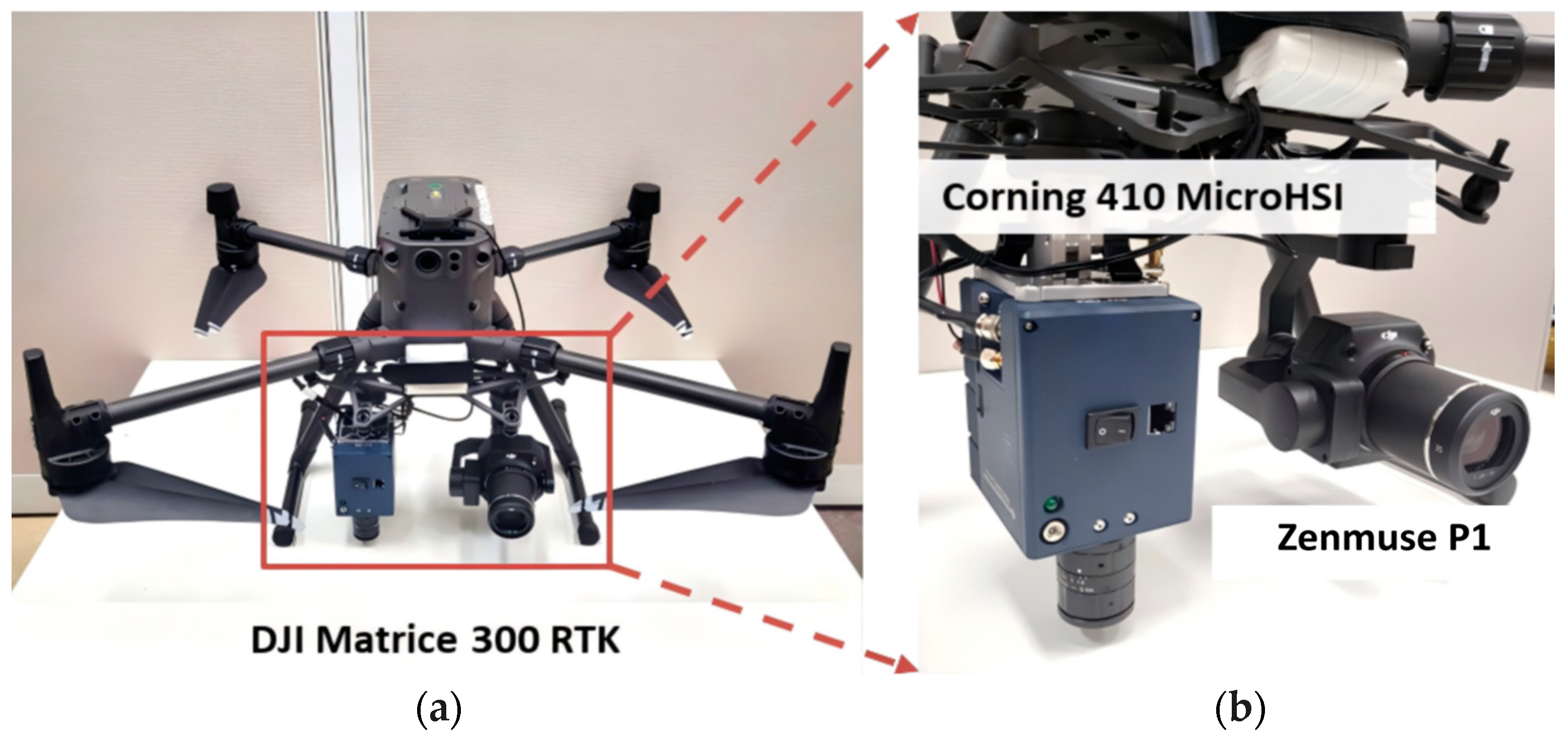
2.2. Instruments and Operations for the Flight Mission

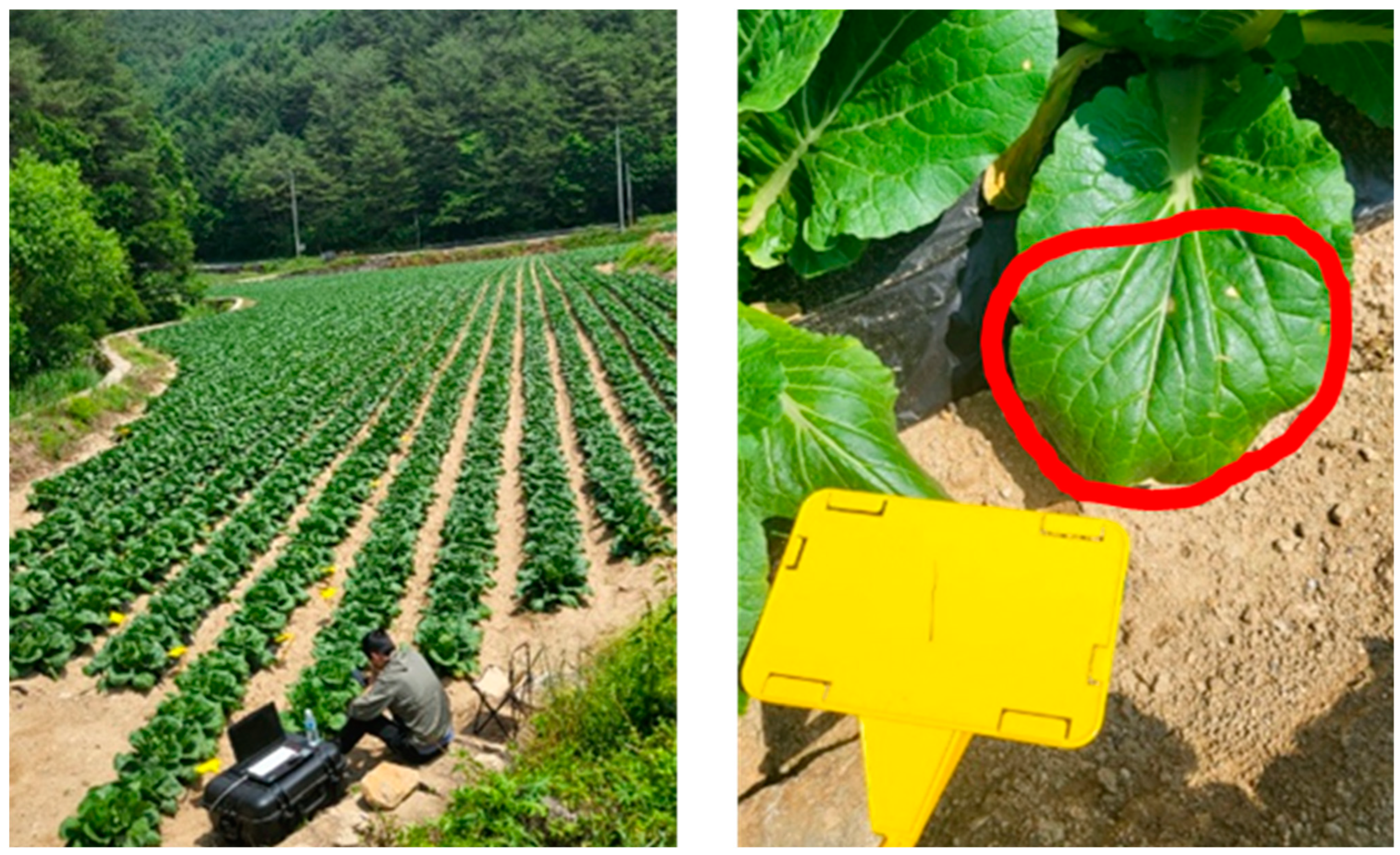
The UAV-based hyperspectral camera system (Figure 2) comprised a Matrice 300 RTK (DJI, Shenzhen, China) as the UAV platform, equipped with two cameras: a Corning 410 MicroHSI hyperspectral camera (Corning Inc., New York, NY, USA) and a Zenmuse P1 RGB camera (DJI, Shenzhen, China). Flight operations were autonomously managed using UgCS 4.0 (SPH Engineering, Riga, Latvia), specialized flight planning software for drones. Both cameras simultaneously captured images of the kimchi cabbage field from a height of 20 m at an average speed of 1.83 m/s. This speed was precisely selected to align with the capturing rate of the hyperspectral camera, ensuring the optimal quality of the hyperspectral images. Additional equipment (Figure 3), including standard reflectance tarps and ground control points (GCPs), were utilized. Four standard calibration tarps (Group 8 Technology, Inc., Provo, UT, USA) with known reflectance values of 3%, 12%, 38%, and 56% were positioned along the perimeter of the field. These tarps facilitated the calibration of the captured hyperspectral images during the subsequent processing steps. GCPs were strategically placed at the corners of the captured fields to facilitate georeferencing. The location of each GCP was determined using an ArduSimple RTK2B-F9P Global Positioning System (GPS) receiver (ArduSimple, Andorra la Vella, Andorra) with an accuracy of 2 cm.

2.3. Ground Survey

A plant disease expert conducted field surveys, examining the kimchi cabbage plants for signs of downy mildew infection. Symptoms such as yellow-tan spots on the upper surface of leaves, small spots, mottling, and grayish spots underneath the leaves were identified as indicative of downy mildew. Yellow markers were placed in the field to indicate the locations of downy mildew-infected plants, as depicted in Figure 4. Ground surveys were carried out twice, on June 12th and 23rd, to monitor the disease progression.

2.4. Preprocessing of the Hyperspectral Images

The acquired hyperspectral data comprised raw digital number (DN) values, which were suboptimal for spectrum analysis. Additionally, image distortions resulting from wind or drone movements required preprocessing steps to render the hyperspectral data usable. In contrast, the preprocessing steps for the RGB images were straightforward. The images were mosaicked using Agisoft Metashape version 1.7.6 (Agisoft LLC., St. Petersburg, Russia) to create a single large-sized image of the studied kimchi cabbage field.

2.4.1. Image Rectification

Data acquisition using line-scanning-type hyperspectral technology demands synchronization between the camera’s capturing rate and the UAV platform’s speed. Throughout the acquisition process, a line of pixels, usually encompassing several spectral bands, was captured and stacked sequentially to produce the hyperspectral images. Minor drifts caused by winds or UAV vibration may result in misalignment within the image. However, the precise camera location and attitude, recorded using the hyperspectral camera’s GPS receiver and inertial measurement unit (IMU) during acquisition, aided in rectifying such misalignments.

2.4.2. Mosaicking

The UAV-based hyperspectral camera system needed to fly close enough to the ground to capture sufficient information about the disease symptoms. Following the flight mission, multiple hyperspectral strips were generated. Unlike snapshot-type cameras, which can utilize established software like Agisoft Metashape, Pix4D, or DJI Terra for mosaicking, the technology for integrating hyperspectral strips from a line-scanning-type camera is still under development. Therefore, in this research, a stitching program was developed by referring to the work of Yi et al. [28] to seamlessly stitch the hyperspectral strips. This program, developed in Python 3.10, could stitch multiple hyperspectral strips and merge them into one large-size image.

2.4.3. Georeferencing

Georeferencing involves assigning geographic information to hyperspectral images. Utilizing the known coordinates of the GCPs, the location of every pixel in an image can be estimated. The mosaicked hyperspectral image was processed for georeferencing in ENVI version 5.3 (Exelis Visual Information Solutions, Boulder, CO, USA), with four GCPs serving as references. Consequently, the image was stretched and reoriented to faithfully depict the actual field.

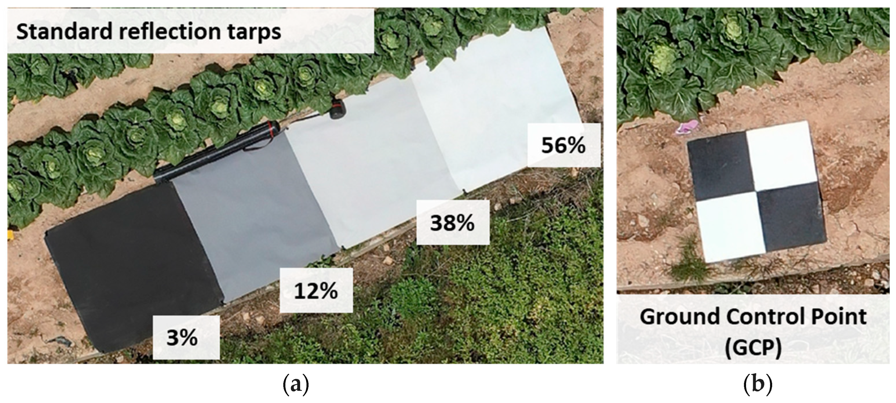
2.4.4. Radiometric Calibration

Observations involving multi-temporal datasets may exhibit variations in radiation due to environmental factors. To mitigate this bias, radiometric calibration, which converts radiation data into reflectance data, is a crucial process. Reflectance values offer a more accurate representation of the biophysical properties of the observed objects and are less susceptible to the variations in radiation. Four standard reflectance tarps were employed for this conversion process, and the calibration was conducted using IDL version 8.5 (Exelis Visual Information Solutions, Boulder, CO, USA). The surface reflectance for each band of the hyperspectral images was calculated using Equations (1) to (3).

$${\rho }_i=m_i · {Ls}_i+b_i$$

(1)

$$m_i={\displaystyle \frac{n(\sum x_j{y}_j)-(\sum x_j\left)\right(\sum y_j) }{n(\sum {x_j}^2)-(\sum {x_j)}^2}}$$

(2)

$$b_i={\displaystyle \frac{\sum y_j-m_i\sum x_j }{n}}$$

(3)

where ${\rho }_i$ represents the reflectance factor, $m_i$ denotes the slope, ${Ls}_i$ signifies the band spectral radiance, $b_i$ represents the bias, and $i$ indicates the spectral band number. Using the computed slope and bias, the remaining pixels in the images were converted into reflectance [29]. Additionally, $x_j$ denotes the average spectral radiance of the tarps, and $y_j$ indicates the known reflectance of the tarps. Here, $j$ represents the tarp number, and $n$ indicates the number of reflectance tarps.

2.5. Defining and Detecting Early Diseases

The downy mildew diseases observed in this study were classified into two stages: early and late. Late-stage diseases exhibited readily visible symptoms, discernible to the human eye, while early-stage diseases presented symptoms that remained undetectable. In this scenario, all the plants marked with yellow markers were categorized as late-stage diseases. Late-stage symptoms appeared as arbitrary-shaped yellow spots on the leaf surface, accompanied by mottling and small spots. To pinpoint early symptoms, a backtracking method was employed. Leveraging geo-information from hyperspectral images, diseased plants could be retraced to their prior state. Before being marked with yellow markers, these plants were deemed to display early symptoms. In this study, hyperspectral bands centered at 450 nm (blue), 550 nm (green), 650 nm (red), and 750 nm (red-edge) were selected for visualization. Early symptoms were more clearly distinguished using a composite of the red-edge, green, and blue (ReGB) bands, as illustrated in Figure 5. The significance of the red-edge band is thoroughly elucidated in the results in Section 3.1. Two flight datasets of the kimchi cabbage field captured at 48 DAS contained early diseased plants, while the flight at 60 DAS featured plants exhibiting late-disease symptoms.

2.6. Spectrum Analysis

The step aimed to comprehend the spectral signature of kimchi cabbage downy mildew by extracting spectral information from healthy areas, areas affected by both late and early stages of the disease, and the background. Here, the background class encompasses the ground and all other objects except kimchi cabbages. To delve deeper into the spectral differences, statistical analysis of variance (ANOVA) was employed using the SciPy library in Python to assess the distinctions between each class. This process entailed comparing the F-values of each class combination across every band.

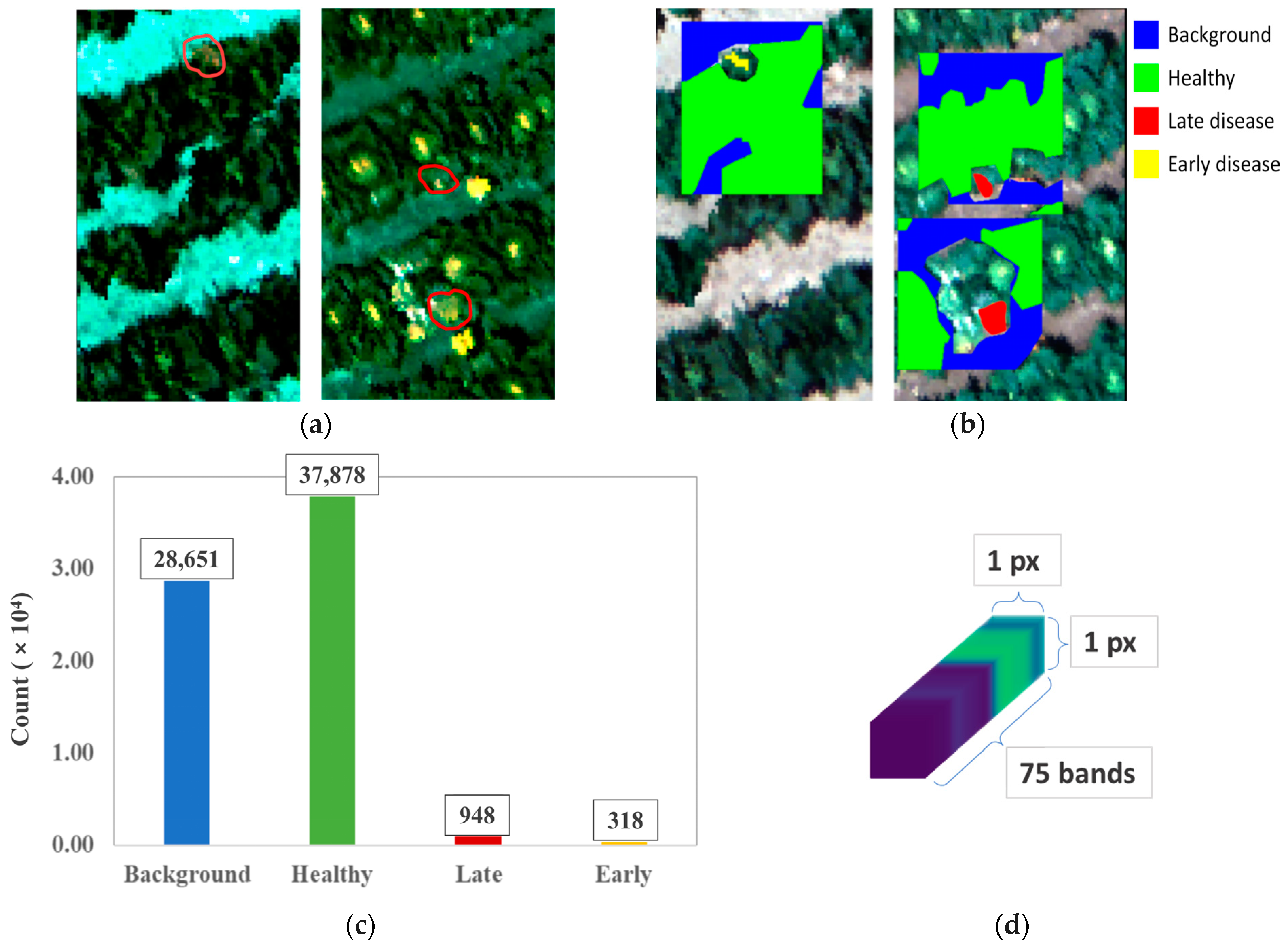
2.7. Establishing the Ground-Truth Dataset Through Labeling

The labeling process entailed categorizing areas surrounding the yellow markers into four distinct classes: background, healthy, late disease, and early disease, which were color-coded as blue, green, red, and yellow, respectively. Background encompassed any objects present in the images other than kimchi cabbage, while the healthy class denoted the unaffected parts of the kimchi cabbage, specifically leaves devoid of any symptoms of downy mildew infection. Late disease areas were those indicated by the expert as having developed symptoms of downy mildew disease, whereas early symptoms referred to areas exhibiting initial signs of the disease. Figure 6 shows a labeled field observed via RGB bands and ReGB bands. Each dataset comprised a series of wavelengths with dimensions of 1 × 1 × 75 bands. In total, the dataset included 67,795 samples, comprising 28,651 background samples, 37,878 healthy samples, 948 late diseased samples, and 318 early diseased samples.

2.8. 1D-CNN and ML Models

2.8.1. Random Forest

Random Forest (RF) is an ML algorithm renowned for its high performance and robustness. RF utilizes decision trees as its core algorithm to generate predictions. However, unlike individual decision trees, which are prone to overfitting, RF employs an ensemble learning approach by combining multiple decision trees. Each node in these trees corresponds to a feature from the input data, and the collective decision from each tree generates a majority vote to generate a prediction. This ensemble method compensates for errors from individual trees, thereby yielding more robust predictions. RF has demonstrated high performance in practice and, in some cases, has achieved comparable results to neural networks. However, like many ML algorithms, RF may encounter difficulties in handling large datasets, and its performance may plateau as the dataset size increases.

2.8.2. 1D-CNN

Unlike traditional ML algorithms, CNNs belong to the realm of DL, where performance typically improves with larger datasets. While CNNs are predominantly used for processing 2D data, they can also be tailored to accommodate 1D signals, enabling the identification of hidden patterns within such data. One of the primary advantages of 1D-CNN is its high speed and low computational cost. In this study, three CNN models were constructed for comparison: a plain 1D-CNN, a 1D-ResNet, and a 1D-InceptionNet model. Each of these models comprised three layers with increasing features. Furthermore, each layer was followed by a rectified linear unit activation (ReLU) function and a maximum pooling (maxpool) layer, as depicted in Figure 7.

The plain 1D-CNN comprised three convolutional layers with 32, 64, and 128 features, respectively. In each layer, convolution processed the values within its input, applying the weights of the kernels element-wise and incorporating bias to produce an output. These layers were arranged sequentially to construct a deeper network and facilitate the learning of more intricate features [30]. Generally, the dimension of the kernel and its convolution axes determine whether it is a 1D-, 2D-, or 3D-CNN. A 1D-CNN possesses a 1D input, kernel, and axis of convolution. In essence, it processes 1D signals, such as spectrum data, into a 1D output representing the class probabilities.

ResNet was first introduced by He et al. [21] to create deeper CNNs. Deep CNNs with numerous hidden layers often suffer from information loss within the network. ResNet addresses this issue by employing residual blocks, which utilize shortcuts to control the information flow and preserve the gradient updates throughout the network during training. This architecture enables the construction of very deep networks while mitigating the risk of overfitting. In this study, a simplified 1D-CNN model was adapted from the ResNet-18 architecture, consisting of three residual blocks with 32, 64, and 128 feature channels, respectively.

The InceptionNet architecture stands out for its use of multiple parallel kernels with varying sizes, referred to as inception blocks, enabling the recognition of features at various scales. Initially introduced by Szegedy et al. [22], it was developed based on the concept of employing sparsely connected architectures to tackle overfitting and computational costs. This design favors wider networks over deeper ones. In this study, the original InceptionNet model was adapted into a 1D-CNN and constructed with three inception blocks, each featuring 32, 64 and 128 features, respectively.

2.9. Experiment Design

In this study, a highly imbalanced dataset was generated, with the background and healthy classes significantly outnumbering the early and late disease classes. Imbalanced datasets can impact the model’s performance because predictions often lean towards the class with more data. To address this concern, the background and healthy classes were downsampled to 20%, 40%, 60%, 80%, and 100% data usage for training. This data composition was applied to the RF, 1D-CNN, 1D-ResNet, and 1D-InceptionNet models. The training process was conducted on a computer equipped with an NVIDIA A4000 RTX 16 GB Graphics Processing Unit (GPU), employing Python 3.10 and PyTorch. The learning rate commenced at 0.003 and degraded every 25 epochs, with a rate decay of 0.5 for a total of 100 epochs. During each epoch, the model’s accuracy and F1 scores were evaluated, and the model with the highest F1 score was saved. To ensure a fair comparison of the model performance, identical training parameters were applied across all the models. The standard cross-entropy loss function (CrossEntropyLoss) was employed for all the deep learning models. The mathematical expressions for accuracy and F1 score were derived from true positive (TP), true negative (TN), false positive (FP), and false negative (FN) values, as outlined in Equations (4) to (7).

$$Accuracy={\displaystyle \frac{TP+TN}{TP+TN+FP+FN}}$$

(4)

$$Precision={\displaystyle \frac{TP}{TP+FN}}$$

(5)

$$Recall={\displaystyle \frac{TP}{TP+FP}}$$

(6)

$$F1={\displaystyle \frac{2\times Precision\times Recall}{Precision+Recall}}$$

(7)

3. Results

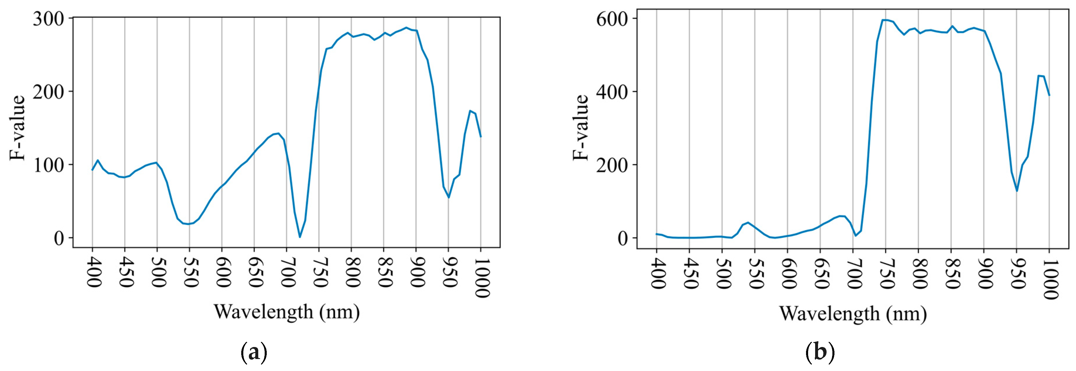
3.1. Spectrum Analysis Results

The spectral data for background, healthy, late disease, and early disease were extracted from the 48 and 60 DAS data, and the color code along with the utilized data is presented in Figure 8a. These spectra were then plotted, as shown in Figure 8b, with solid lines representing the average spectrum data and the colored areas depicting the spectral variance of each class. Notably, the background class exhibited the most pronounced difference compared to the other classes, characterized by low reflectance, ranging between 0 and 0.5, across the spectrum. Upon examining the average reflectance of each class, healthy leaves showed a high NIR reflectance of approximately 0.68, whereas late diseased leaves exhibited a lower NIR reflectance of approximately 0.62. Conversely, the reflectance of healthy leaves in the blue (450 nm), green (550 nm), and red-edge (750 nm) bands was lower than that of the late diseased leaves; healthy leaves exhibited reflectance values of 0.03, 0.14, and 0.4, while late diseased leaves exhibited reflectance values of 0.05, 0.16, and 0.5, respectively. Early diseased leaves exhibited reflectance values comparable to that of healthy leaves throughout the spectrum, except in the red-edge band (750 nm), where early diseased leaves exhibited a slightly higher red-edge reflectance of 0.5, compared to healthy leaves with a reflectance of 0.4.

Further analysis using ANOVA was conducted to thoroughly examine the variance in the data. The analysis involved comparing the F-values across the spectrum of class combinations, as illustrated in Figure 9. The F-value serves as an indicator of the dissimilarity between datasets. Given the large sample sizes and high degrees of freedom, the resulting p-values were extremely small. Notably, an F-value greater than 10.83 corresponded to a significance level of p < 0.001, indicating a statistically significant difference between the compared classes. The results indicated significant differences between the background class and the other classes in the NIR range. As shown in Figure 9a–c, the NIR band between 750 and 900 nm exhibited high F-values of 290, 600, and 950 for comparisons between the background class and the healthy, early disease, and late disease classes, respectively. Discrepancies in the visible and red-edge bands were observed between the healthy and late classes, indicating noticeable discoloration and a reduction in the leaf chlorophyll content in the late disease class. As shown in Figure 9d, the F-values in the visible bands, consisting of blue (450 nm), green (550 nm), and red (650 nm) bands, were 220, 290, and 120, respectively. Furthermore, the highest F-value of 320 was observed in the red-edge band (720 nm). In Figure 9e, peak differences in the red-edge band, particularly at 720 nm, with an F-value of 340, were observed between the healthy and early classes, indicating a depletion in chlorophyll content. This finding highlights the potential of this specific band as a key indicator of the early symptoms of downy mildew disease. The differences in the visible and NIR bands between the early and late classes, presented in Figure 9f, illustrated the gradual development of downy mildew and its substantial impact on the leaf cell structure. Furthermore, intriguing results were observed in the water bands (950–1000 nm), suggesting a lower water content during late disease symptoms.

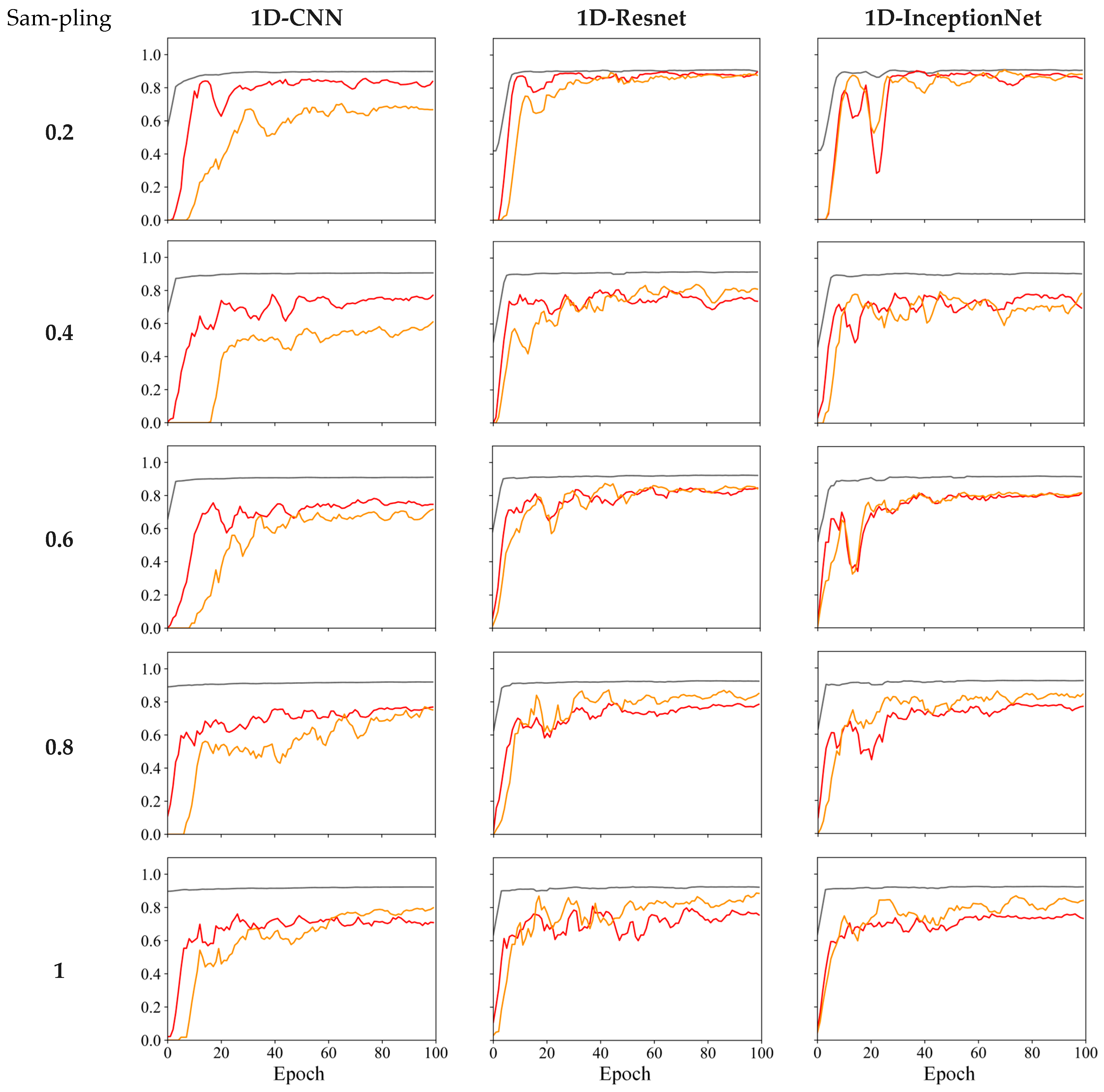
3.2. Training Process for Each Model

The 1D-CNN, 1D-ResNet, and 1D-InceptionNet models were trained for 100 epochs at an initial learning rate of 10⁻³, which decreased by a rate decay of 0.5 every 25 epochs. Different sampling compositions of 0.2, 0.4, 0.6, 0.8, and 1 were utilized for training, with sampling focusing on undersampling only the background and healthy classes due to their significant imbalances. The overall testing accuracy, along with early and late disease classification accuracies, were plotted in gray, red, and orange colors, respectively (Figure 10).

In terms of training performance, 1D-ResNet and 1D-InceptionNet demonstrated more effective learning of early and late disease classifications. For instance, when comparing the training performance at 0.2 sampling, both early and late disease prediction accuracies reached approximately 0.75 at 20 epochs, whereas 1D-CNN fell short of even reaching 0.7. Notably, 1D-InceptionNet exhibited fluctuations in the early stages of training, in contrast to the consistent progress observed with 1D-ResNet. For example, in a 0.2 sampling dataset, between epochs 10 and 25, the accuracy of late and early disease classifications by the 1D-InceptionNet model fluctuated between 0.25 and 0.82, whereas that of classification by the 1D-ResNet model fluctuated between 0.70 and 0.82. The fluctuation in 1D-InceptionNet’s learning may be attributed to the varying sizes and numbers of kernels present in its inception layers, resulting in initial instability followed by stabilization over time. Given that the models were trained on an imbalanced dataset, the selection of the best model was based on the highest F1 score, which balances the effects of the majority class by incorporating both precision and recall [31].

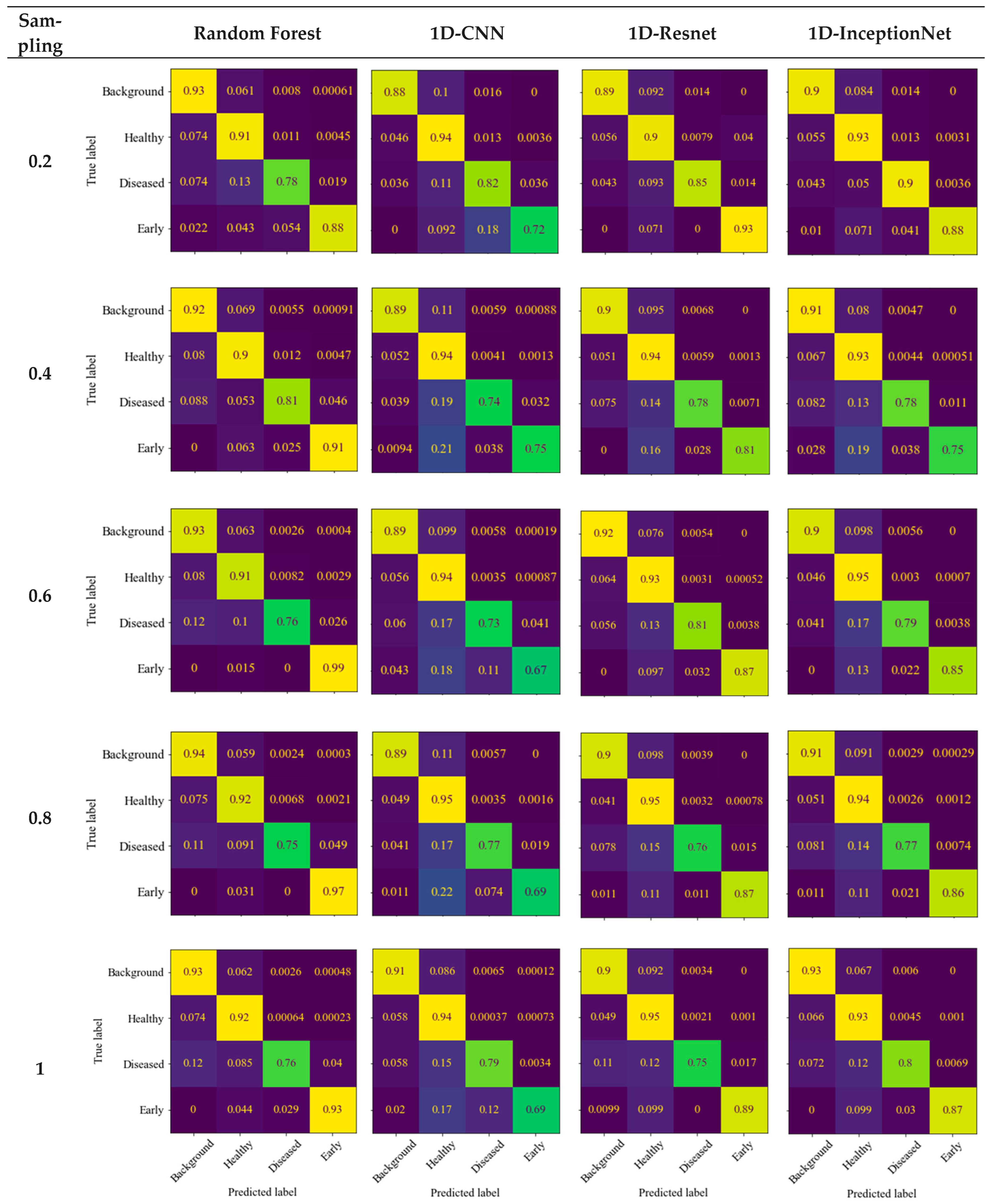
3.3. Comparing Each Model’s Performance and Generating Confusion Matrices

Table 1. The accuracy of the healthy, late disease, and early disease classifications, as well as the overall accuracy and F1 scores of RF, 1D-CNN, 1D-ResNet, and 1D-InceptionNet for each dataset sampling.

CNN Architecture	Dataset Sampling	Healthy Class	Late Disease Class	Early Disease Class	Overall Accuracy	F1 Score
RF	0.2	0.913	0.777	0.882	0.907	0.876
	0.4	0.902	0.813	0.911	0.909	0.848
	0.6	0.913	0.758	0.985	0.916	0.859
	0.8	0.924	0.755	0.969	0.923	0.847
	1	0.924	0.758	0.926	0.922	0.831
1D-CNN	0.2	0.882	0.826	0.721	0.901	0.845
	0.4	0.893	0.747	0.752	0.907	0.849
	0.6	0.891	0.731	0.676	0.919	0.835
	0.8	0.896	0.774	0.697	0.914	0.832
	1	0.919	0.798	0.694	0.921	0.835
1D-ResNet	0.2	0.893	0.854	0.934	0.909	0.897
	0.4	0.906	0.782	0.812	0.914	0.875
	0.6	0.923	0.814	0.876	0.923	0.893
	0.8	0.905	0.763	0.877	0.924	0.878
	1	0.902	0.753	0.892	0.924	0.876
1D-InceptionNet	0.2	0.908	0.905	0.883	0.914	0.899
	0.4	0.914	0.787	0.755	0.914	0.870
	0.6	0.901	0.798	0.852	0.921	0.885
	0.8	0.913	0.772	0.861	0.923	0.877
	1	0.933	0.805	0.872	0.925	0.873

presents the accuracy of the healthy, late disease, and early disease classifications, as well as the overall accuracy and F1 scores of RF, 1D-CNN, 1D-ResNet, and 1D-InceptionNet across the various dataset samplings. For simplicity, the table excludes the display of background class predictions, as all the models demonstrated high accuracy in this regard.

Figure 11 shows the confusion matrices of all the models, including RF, across various samplings. Surprisingly, RF exhibited slightly better performance than the 1D-CNN model. In datasets with the sampling rates of 0.2, 0.6, and 0.8, RF achieved marginally higher F1 scores compared to 1D-CNN. Additionally, RF outperformed 1D-CNN in classifying early disease, with F1 scores of 0.882, 0.911, 0.985, 0.969, and 0.926 for the 0.2, 0.4, 0.6, 0.8, and 1 sampling datasets, respectively, whereas 1D-CNN achieved F1 scores of 0.721, 0.752, 0.676, 0.697, and 0.694, respectively.

On the other hand, the late disease prediction accuracy of the RF and 1D-CNN models remained nearly identical across all the sampling datasets, ranging from 0.731 to 0.826. The 1D-ResNet and 1D-InceptionNet models demonstrated superior overall performance, displaying high and well-balanced accuracies across all four classes, resulting in higher F1 scores. Interestingly, the F1 scores decreased while the overall accuracy increased with higher sampling rates. This phenomenon can be attributed to the majority of the dataset being composed of background and healthy samples, which are easier to predict and, consequently, contribute to higher overall accuracy. However, F1 scores provided a better representation of model performance because they consider each class’s prediction accuracy while balancing the dataset.

Comparing the model performances across different dataset samplings demonstrated that all the models performed relatively poorer on imbalanced datasets. Nonetheless, 1D-ResNet and 1D-InceptionNet consistently maintained notably high F1 scores even on highly imbalanced datasets. For the 0.2 sampling dataset, RF, 1D-CNN, 1D-ResNet, and 1D-InceptionNet achieved F1 scores of 0.831, 0.835, 0.876, and 0.873, respectively.

Typically, a balanced dataset yields a high-performance model. Therefore, the dataset with a sampling rate of 0.2 was considered the most favorable. In this scenario, 1D-InceptionNet outperformed all the other models with an F1 score of 0.899, while 1D-ResNet, 1D-CNN, and RF attained F1 scores of 0.897, 0.845, and 0.848, respectively. Therefore, the optimal model in this study was determined to be 1D-InceptionNet with a 0.2 dataset sampling.

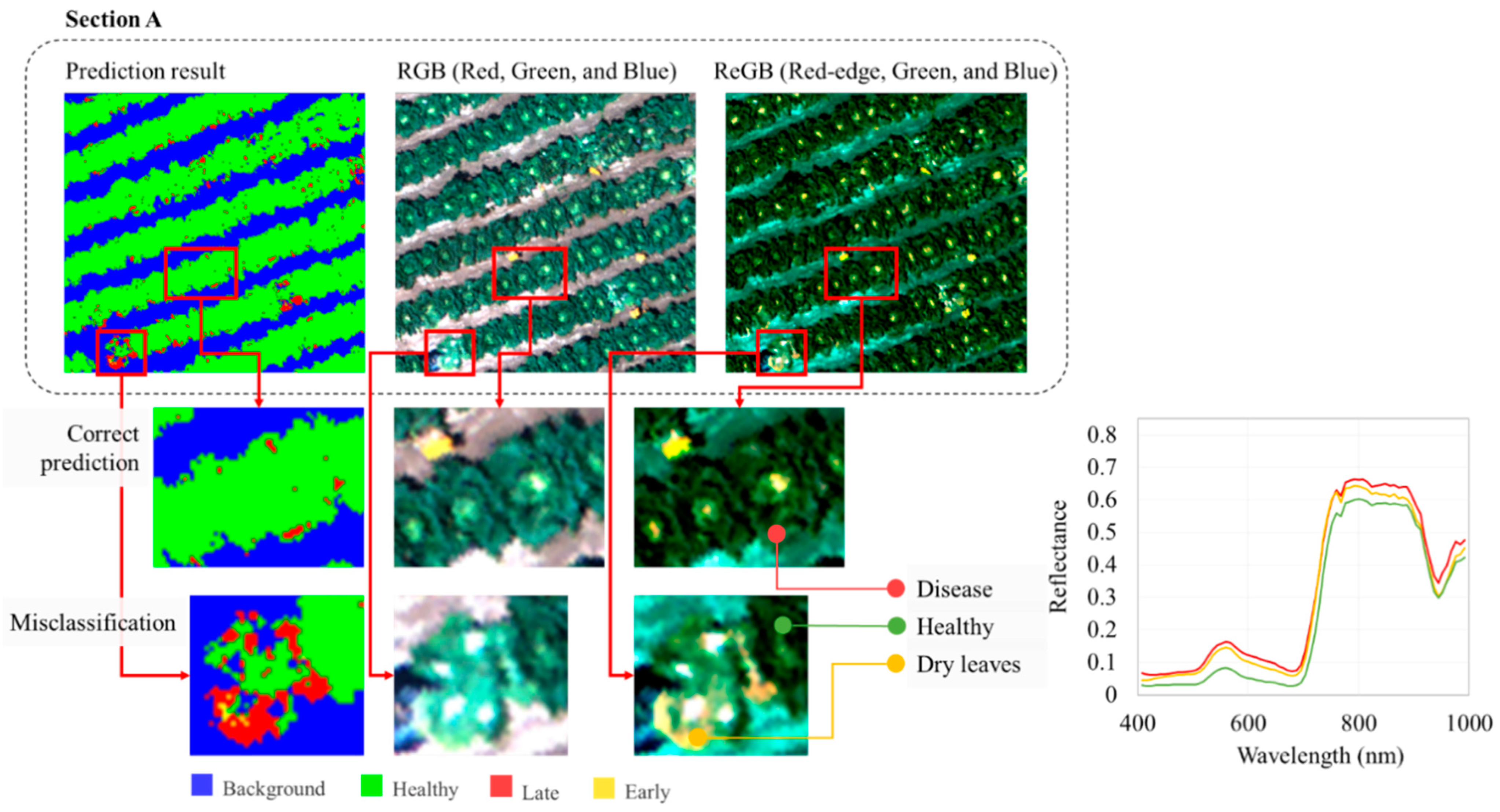
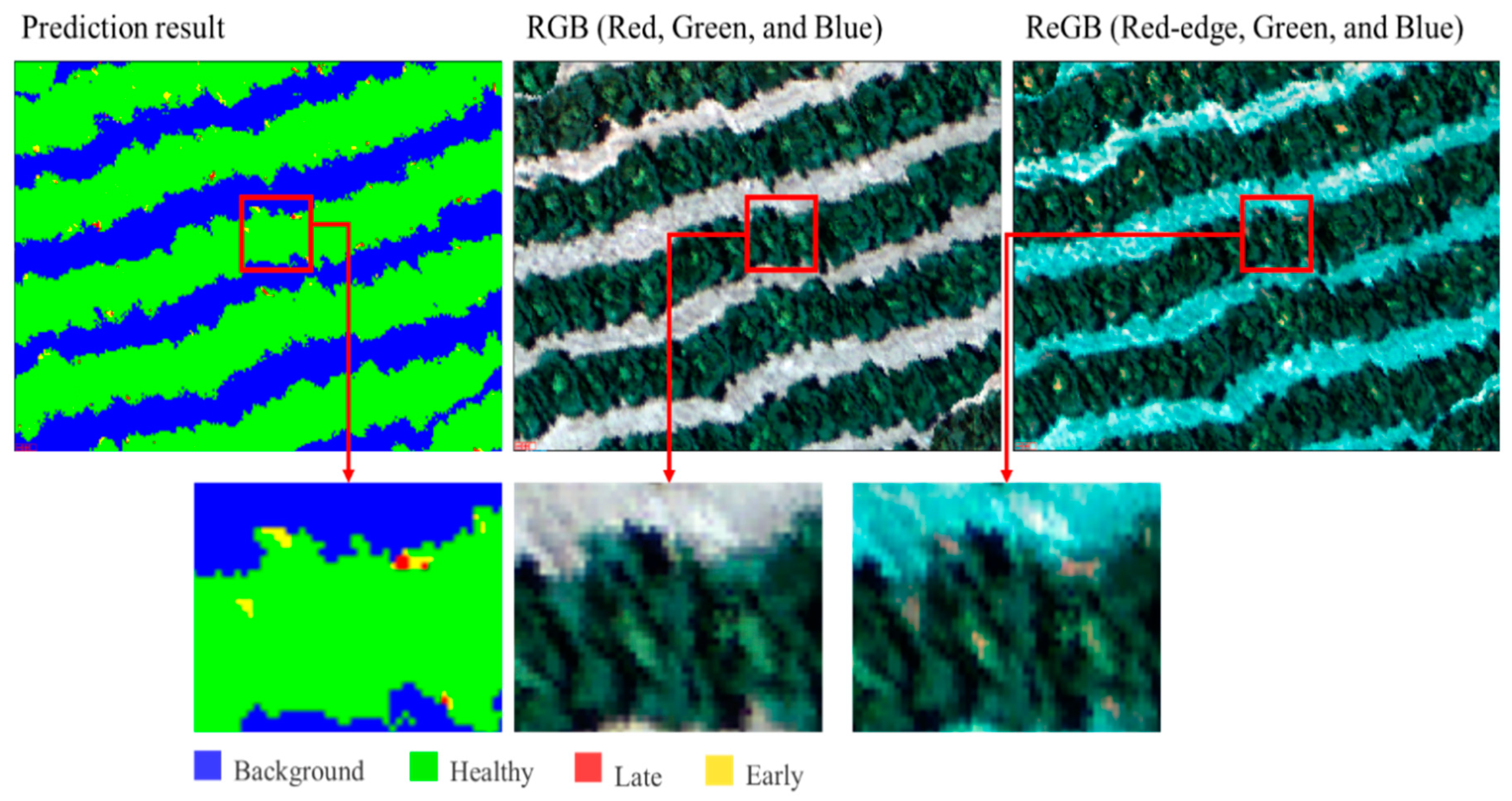
3.4. Visualization of the Prediction Results

Figure 12 illustrates the prediction results of the studied field at 60 DAS, with background, healthy, late disease, and early disease classes represented in blue, green, red, and yellow colors, respectively. Additionally, a detailed view (Section A) of the prediction results at 60 DAS, along with the ReGB and RGB images of the field is presented in Figure 13. Similarly, Figure 14 provides a detailed view of the prediction results at 48 DAS, along with the ReGB and RGB images of the field. The yellow or orange coloration observed in the outer leaves in the ReGB and RGB images corresponds to the areas affected by downy mildew. The features apparent in both the ReGB and RGB images align with the prediction results, indicating that the model has effectively learned the relevant features associated with downy mildew infection. This visual confirmation further validates the accuracy of the model in identifying the diseased areas within the kimchi cabbage field.

Although misclassifications or false positives of late or early disease did occur, they were primarily caused by dead or dried leaves. The spectrum of dried or dead leaves may share similarities with late-stage disease symptoms. As evident in the spectral plot in Figure 13, where the similarities are obvious in the visible band, the diseased leaves exhibited reflectance values of 0.06, 0.16, and 0.1, whereas the dried leaves exhibited reflectance values of 0.05, 0.15, and 0.08 in the 450, 550, and 650 nm regions, respectively. To tackle this challenge, incorporating dried leaves into the training dataset as background and augmenting the model with additional spatial information could be a potential solution to obtain contextual clues for image analysis.

4. Discussion

4.1. Data Acquisition Results and Challenges

Maintaining an optimal altitude during flight missions was crucial for capturing sharp hyperspectral images with the desired ground sample distance (GSD). To accommodate the uneven terrain, the flight mission employed a terrain-following mode, ensuring a consistent altitude above ground level (AGL) [32]. In this instance, the UAV was maintained at 20 AGL to guarantee GSDs of 1.2 cm and 0.25 cm for the hyperspectral and high-resolution RGB cameras, respectively.

The timing for data acquisition was meticulously chosen to ensure optimal lighting conditions. Natural sunlight was utilized as the primary light source for capturing hyperspectral images. Flight missions were scheduled between 11 am and 1 pm to coincide with the sun being directly overhead, minimizing cast shadows and ensuring sufficient sun radiation [33]. Conducting flights earlier or later in the day posed a risk of casting excessive shadows, which could potentially obscure disease symptoms. Additionally, days with minimal cloud cover were preferred to avoid reductions in illumination that could lead to noisy images.

Obtaining an adequate number of diseased samples was crucial for model development. However, the natural occurrence of diseases, influenced by external factors, such as field location, seasons, temperature, and humidity, presented challenges in controlling and predicting the disease occurrence. Often, the number of diseased samples was limited and sporadic. Given the high dimensionality of the hyperspectral imaging data and the necessity for sufficient data to ensure model generalization, addressing these challenges was paramount for successful model development [34].

4.2. Kimchi Cabbage Downy Mildew Spectrum Signature

In this study, the red-edge band played a crucial role in indicating downy mildew disease symptoms in kimchi cabbages. While a slightly higher reflectance in the red-edge band can suggest a reduction in the chlorophyll content, considering other factors that might contribute to this observation is essential [35]. Downy mildew infection can cause a decline in chlorophyll cells, thereby impacting the overall reflectance properties of the plant leaves. However, variations in the chlorophyll content can also arise from factors unrelated to disease infection, such as different growth stages of the plant or nutritional deficiencies.

To comprehensively understand downy mildew development in kimchi cabbages, it may be necessary to conduct a thorough study encompassing various growth stages and nutritional conditions. This approach would help distinguish disease-induced changes in the chlorophyll content from those caused by other factors, such as nutrition and growth stage. Analyzing the spectral signatures of the plant at different stages and under different conditions would enable researchers to better identify the specific indicators of downy mildew infection and enhance the accuracy of the disease detection methods.

Parasitic fungi, including H. brassicae, which cause downy mildew in kimchi cabbages, grow by penetrating the host cells using haustoria, a highly modified structure that extends from the hypha through small pores in the cell wall to facilitate the nutrient absorption from the plant [36]. This process explains why downy mildew initially causes chlorophyll loss, as indicated by changes in the red-edge band. Continuous infestation eventually leads to the destruction of leaf cells, as indicated by a decrease in the NIR range, which is commonly associated with changes in the cell structure.

In addition to spectral features, spatial characteristics, such as shape and texture, also serve as indicators of downy mildew diseases. The irregular shape of yellow spots and the distinct contrast between infected and healthy areas are notable spatial features of downy mildew symptoms. High-resolution RGB images capture these spatial features more prominently than hyperspectral images due to their finer resolution and detail. Furthermore, while pixel-level segmentation is effective in generating large amounts of data, it may overlook spatial features that could provide valuable information for disease detection and classification. Therefore, incorporating spatial analysis techniques with spectral analysis approaches—such as combining 1D spectral models with 2D CNNs or Transformer-based spatial modules—could further improve the accuracy and robustness of the disease detection methods. Additionally, integrating endmember collection techniques is planned for future research to enhance the model’s ability to more effectively differentiate between early- and late-stage disease symptoms.

4.3. Comparison with the Previous Study

This study builds upon our previous study [26], which employed a 3D-CNN. However, in the current investigation, such an approach was not feasible due to insufficient disease samples. A comparison of approaches and results between this study and the previous one is presented in

Table 2. Summary of the field conditions, approaches, and findings of our previous [26] and current studies.

Parameters	Previous Study	Current Study
Crops	Autumn cabbage	Spring cabbage
Disease occurrence	High disease incidence	Low disease incidence
Illumination condition	Diffused illumination (obscured by the shadows of the surrounding mountains)	Direct illumination
Segmentation method	Leaf level	Pixel level
Data dimension	20 × 20 × 55 (difficult to train)	1 × 1 × 75 (easier to train)
Dataset number	Sparse data	Extensive data
Model	2D-ResNet, 3D-ResNet 1, 3D-ResNet 2	RF, 1D-CNN, 1D-ResNet, 1D-InceptionNet
Robustness	Robust to noise	Prone to noise
Output prediction	Background, healthy, diseased	Background, healthy, early, late
Overall accuracy	0.876	0.914

. The focus of this study was on spring kimchi cabbages, with data acquisition conducted under direct sunlight, resulting in bright images but less contrast in the disease symptoms. In contrast, the previous study, conducted in the autumn, captured images under the shade of the surrounding mountains, resulting in more apparent disease symptoms but less illumination.

In the previous study, kimchi cabbage images were segmented into smaller leaf patches using the SLIC segmentation algorithm, resulting in a complex dataset with higher dimensions. Despite having fewer datasets, it was robust to noise, had dimensions of 20 × 20 × 55, and was trained using 2D-ResNet, 3D-ResNet 1, and 3D-ResNet 2. In contrast, pixel-level segmentation was employed in this study, resulting in more datasets but lesser complexity and higher susceptibility to noise. Leaf-level segmentation was not possible due to a lack of sufficient diseased samples, resulting in a 1D dataset of 1 × 1 × 75, which was fed into RF, 1D-CNN, 1D-ResNet, and 1D-InceptionNet for training. Both studies demonstrated high accuracy in detecting diseases in their respective fields, with an emphasis on the red-edge band as the most influential aspect. To ensure prediction reliability, these models must be tested in various kimchi cabbage fields during different growing periods.

4.4. Implications

Identifying plant diseases through symptom inspection remains the gold standard, as recommended by the relevant authorities. However, this method presents several drawbacks, including the requirement for trained personnel, high costs, and lengthy processing times [3]. Moreover, relying solely on symptomatic infections can lead to delayed intervention, allowing diseases to cause varying degrees of damage before detection. Early symptoms often elude human observation. Additionally, pathogen determination is prone to bias and relies on expert interpretation [37].

The early detection of plant disease infection is crucial for disease control. Accurate early disease detection facilitates rapid treatment, minimizing plant damage and reducing losses, significantly benefiting farmers and the agricultural sector as a whole [38]. Drones and aerial survey technologies facilitate large-scale operations and accurate mapping to precisely identify diseased locations, allowing for the selective treatment of plants and thereby reducing labor and pesticide usage. However, implementing this approach requires collaboration across various disciplines. Identifying and sensing diseased plants is a crucial step in this direction. However, research exploring the spectral signature of downy mildew on kimchi cabbages is still in the early stages, with only a few research publications available.

5. Conclusions

This study successfully developed an automatic detection system for downy mildew disease in kimchi cabbages. This system comprises airborne hyperspectral camera data processing software and prediction models. It offers a promising alternative to traditional disease detection methods, which are often inefficient and inconsistent. By leveraging the extensive spectral information provided by hyperspectral cameras, this system enables the efficient and accurate detection of downy mildew infection in kimchi cabbages. Spectrum analysis showed that the red-edge band serves as a reliable indicator for both early- and late-stage diseases. Four ML models, namely RF, 1D-CNN, 1D-ResNet, and 1D-InceptionNet, were developed. Due to the dataset’s imbalance, experiments were conducted to determine the best-performing model using sampling datasets of 0.2, 0.4, 0.6, 0.8, and 1. The 1D-InceptionNet emerged as the top-performing model with an F1 score of 0.899 and an overall accuracy of 0.914. Meanwhile, RF, 1D-CNN, and 1D-ResNet achieved F1 scores of 0.876, 0.845, and 0.897, respectively, with overall accuracies of 0.907, 0.901, and 0.909. While the 1D-InceptionNet exhibited impressive performance, it overlooked crucial spatial features, such as texture, contrasts, and contextual information from neighboring pixels.

Future research efforts should prioritize the development of models capable of effectively processing both spectral and spatial information. Furthermore, the dependence on substantial datasets for developing DL models underscores the importance of the ongoing data collection efforts in the field. Gathering more in-field data will not only enhance the model’s performance but also make it more robust and reliable. Furthermore, optimizing the model for deployment on edge devices will facilitate real-time disease detection and strengthen its generalization across diverse agricultural conditions.

References

1. Lee, H.J.; Lee, J.S.; Choi, Y.J. New downy mildew disease caused by Hyaloperonospora brassicae on Pak choi (Brassica rapa) in Korea. Res. Plant Dis. 2019, 25, 99. [Google Scholar] [CrossRef]
2. Niu, X.; Leung, H.; Williams, P.H. Sources and Nature of Resistance to Downy Mildew and Turnip Mosaic in Chinese Cabbage. J. Am. Soc. Hortic. Sci. 1983, 108, 775–778. [Google Scholar] [CrossRef]
3. Buja, I.; Sabella, E.; Monteduro, A.G.; Chiriacò, M.S.; De Bellis, L.; Luvisi, A.; Maruccio, G. Advances in Plant Disease Detection and Monitoring: From Traditional Assays to In-Field Diagnostics. Sensors 2021, 21, 2129. [Google Scholar] [CrossRef] [PubMed]
4. Barbedo, J. A Review on the Use of Unmanned Aerial Vehicles and Imaging Sensors for Monitoring and Assessing Plant Stresses. Drones 2019, 3, 40. [Google Scholar] [CrossRef]
5. Selci, S. The Future of Hyperspectral Imaging. J. Imaging 2019, 5, 84. [Google Scholar] [CrossRef]
6. Jung, D.-H.; Kim, J.D.; Kim, H.-Y.; Lee, T.S.; Kim, H.S.; Park, S.H. A Hyperspectral Data 3D Convolutional Neural Network Classification Model for Diagnosis of Gray Mold Disease in Strawberry Leaves. Front. Plant Sci. 2022, 13, 837020. [Google Scholar] [CrossRef]
7. Kuswidiyanto, L.W.; Noh, H.-H.; Han, X. Plant Disease Diagnosis Using Deep Learning Based on Aerial Hyperspectral Images: A Review. Remote Sens. 2022, 14, 6031. [Google Scholar] [CrossRef]
8. Wan, L.; Li, H.; Li, C.; Wang, A.; Yang, Y.; Wang, P. Hyperspectral Sensing of Plant Diseases: Principle and Methods. Agronomy 2022, 12, 1451. [Google Scholar] [CrossRef]
9. Singh, P.; Pandey, P.C.; Petropoulos, G.P.; Pavlides, A.; Srivastava, P.K.; Koutsias, N.; Deng, K.A.K.; Bao, Y. Hyperspectral remote sensing in precision agriculture: Present status, challenges, and future trends. In Hyperspectral Remote Sensing; Elsevier: Amsterdam, The Netherlands, 2020; pp. 121–146. [Google Scholar] [CrossRef]
10. Mishra, P.; Asaari, M.S.M.; Herrero-Langreo, A.; Lohumi, S.; Diezma, B.; Scheunders, P. Close range hyperspectral imaging of plants: A review. Biosyst. Eng. 2017, 164, 49–67. [Google Scholar] [CrossRef]
11. Carter, G.A.; Knapp, A.K. Leaf optical properties in higher plants: Linking spectral characteristics to stress and chlorophyll concentration. Am. J. Bot. 2001, 88, 677–684. [Google Scholar] [CrossRef]
12. Fernández, C.I.; Leblon, B.; Wang, J.; Haddadi, A.; Wang, K. Cucumber Powdery Mildew Detection Using Hyperspectral Data. Can. J. Plant Sci. 2022, 102, 20–32. [Google Scholar] [CrossRef]
13. Song, H.; Yoon, S.-R.; Dang, Y.-M.; Yang, J.-S.; Hwang, I.M.; Ha, J.-H. Nondestructive classification of soft rot disease in napa cabbage using hyperspectral imaging analysis. Sci. Rep. 2022, 12, 14707. [Google Scholar] [CrossRef] [PubMed]
14. Guo, A.; Huang, W.; Dong, Y.; Ye, H.; Ma, H.; Liu, B.; Wu, W.; Ren, Y.; Ruan, C.; Geng, Y. Wheat yellow rust detection using UAV-based hyperspectral technology. Remote Sens. 2021, 13, 123. [Google Scholar] [CrossRef]
15. Ma, H.; Huang, W.; Dong, Y.; Liu, L.; Guo, A. Using UAV-Based Hyperspectral Imagery to Detect Winter Wheat Fusarium Head Blight. Remote Sens. 2021, 13, 3024. [Google Scholar] [CrossRef]
16. Krichen, M. Convolutional Neural Networks: A Survey. Computers 2023, 12, 151. [Google Scholar] [CrossRef]
17. Liakos, K.; Busato, P.; Moshou, D.; Pearson, S.; Bochtis, D. Machine Learning in Agriculture: A Review. Sensors 2018, 18, 2674. [Google Scholar] [CrossRef]
18. Agarwal, M.; Gupta, S.; Biswas, K.K. A new Conv2D model with modified ReLU activation function for identification of disease type and severity in cucumber plant. Sustain. Comput. Inform. Syst. 2021, 30, 100473. [Google Scholar] [CrossRef]
19. Latif, G.; Abdelhamid, S.E.; Mallouhy, R.E.; Alghazo, J.; Kazimi, Z.A. Deep Learning Utilization in Agriculture: Detection of Rice Plant Diseases Using an Improved CNN Model. Plants 2022, 11, 2230. [Google Scholar] [CrossRef]
20. Fang, X.; Zhen, T.; Li, Z. Lightweight Multiscale CNN Model for Wheat Disease Detection. Appl. Sci. 2023, 13, 5801. [Google Scholar] [CrossRef]
21. He, K.; Zhang, X.; Ren, S.; Sun, J. Deep Residual Learning for Image Recognition. In Proceedings of the IEEE Conference on Computer Vision and Pattern Recognition, Las Vegas, NV, USA, 27–30 June 2016; pp. 770–778. [Google Scholar] [CrossRef]
22. Szegedy, C.; Liu, W.; Jia, Y.; Sermanet, P.; Reed, S.; Anguelov, D.; Erhan, D.; Vanhoucke, V.; Rabinovich, A. Going deeper with convolutions. In Proceedings of the IEEE Conference on Computer Vision and Pattern Recognition, Boston, MA, USA, 7–12 June 2015; pp. 1–9. [Google Scholar] [CrossRef]
23. Kiranyaz, S.; Avci, O.; Abdeljaber, O.; Ince, T.; Gabbouj, M.; Inman, D.J. 1D convolutional neural networks and applications: A survey. Mech. Syst. Signal Process. 2021, 151, 107398. [Google Scholar] [CrossRef]
24. Li, H.; Chen, L.; Yao, Z.; Li, N.; Long, L.; Zhang, X. Intelligent Identification of Pine Wilt Disease Infected Individual Trees Using UAV-Based Hyperspectral Imagery. Remote Sens. 2023, 15, 3295. [Google Scholar] [CrossRef]
25. Deng, J.; Zhang, X.; Yang, Z.; Zhou, C.; Wang, R.; Zhang, K.; Lv, X.; Yang, L.; Wang, Z.; Li, P.; et al. Pixel-level regression for UAV hyperspectral images: Deep learning-based quantitative inverse of wheat stripe rust disease index. Comput. Electron. Agric. 2023, 215, 108434. [Google Scholar] [CrossRef]
26. Kuswidiyanto, L.W.; Wang, P.; Noh, H.H.; Jung, H.Y.; Jung, D.H.; Han, X. Airborne Hyperspectral Imaging for Early Diagnosis of Kimchi Cabbage Downy Mildew Using 3D-ResNet and Leaf Segmentation. Comput. Electron. Agric. 2023, 214, 108312. [Google Scholar] [CrossRef]
27. Terentev, A.; Dolzhenko, V.; Fedotov, A.; Eremenko, D. Current State of Hyperspectral Remote Sensing for Early Plant Disease Detection: A Review. Sensors 2022, 22, 757. [Google Scholar] [CrossRef]
28. Yi, L.; Chen, J.M.; Zhang, G.; Xu, X.; Ming, X.; Guo, W. Seamless mosaicking of uav-based push-broom hyperspectral images for environment monitoring. Remote Sens. 2021, 13, 4720. [Google Scholar] [CrossRef]
29. Mamaghani, B.; Saunders, M.G.; Salvaggio, C. Inherent Reflectance Variability of Vegetation. Agriculture 2019, 9, 246. [Google Scholar] [CrossRef]
30. Polat, K.; Öztürk, Ş. Diagnostic Biomedical Signal and Image Processing Applications with Deep Learning Methods; Intelligent Data-Centric Systems; Academic Press: San Diego, CA, USA, 2023. [Google Scholar] [CrossRef]
31. Orozco-Arias, S.; Piña, J.S.; Tabares-Soto, R.; Castillo-Ossa, L.F.; Guyot, R.; Isaza, G. Measuring performance metrics of machine learning algorithms for detecting and classifying transposable elements. Processes 2020, 8, 638. [Google Scholar] [CrossRef]
32. Trajkovski, K.K.; Grigillo, D.; Petrovic, D. Optimization of UAV Flight Missions in Steep Terrain. Remote Sens. 2020, 12, 1293. [Google Scholar] [CrossRef]
33. Barbosa, M.R.; Tedesco, D.; Carreira, V.D.; Pinto, A.A.; Moreira, B.; Shiratsuchi, L.S.; Zerbato, C.; Da Silva, R.P. The Time of Day Is Key to Discriminate Cultivars of Sugarcane upon Imagery Data from Unmanned Aerial Vehicle. Drones 2022, 6, 112. [Google Scholar] [CrossRef]
34. Chang, K.; Balachandar, N.; Lam, C.; Yi, D.; Brown, J.; Beers, A.; Rosen, B.; Rubin, D.L.; Kalpathy-Cramer, J. Distributed Deep Learning Networks among Institutions for Medical Imaging. J. Am. Med. Inform. Assoc. 2018, 25, 945–954. [Google Scholar] [CrossRef]
35. Gitelson, A.A.; Merzlyak, M.N.; Lichtenthaler, H.K. Detection of red edge position and chlorophyll content by reflectance measurements near 700 nm. J. Plant Physiol. 1996, 148, 501–508. [Google Scholar] [CrossRef]
36. Struck, C.; Cooke, B.M.; Jones, D.G.; Kaye, B. Infection Strategies of Plant Parasitic Fungi. In The Epidemiology of Plant Diseases; Springer: Berlin/Heidelberg, Germany, 2006; pp. 117–137. [Google Scholar] [CrossRef]
37. Riley, M.; Williamson, M.; Maloy, O. Plant Disease Diagnosis. Plant Health Instr. 2002, 10, 193–210. [Google Scholar] [CrossRef]
38. Martinelli, F.; Scalenghe, R.; Davino, S.; Panno, S.; Scuderi, G.; Ruisi, P.; Villa, P.; Stroppiana, D.; Boschetti, M.; Goulart, L.R.; et al. Advanced methods of plant disease detection. A review. Agron. Sustain. Dev. 2015, 35, 1–25. [Google Scholar] [CrossRef]
Figure 1. Research area map indicating the data acquisition sites.
Remotesensing 17 01626 g001
Figure 2. The airborne unmanned aerial vehicle (UAV) data acquisition system with (a) a DJI Matrice 300 RTK as the UAV platform and (b) two cameras—a Corning 410 MicroHSI hyperspectral camera and a Zenmuse P1 RGB camera—for capturing images.
Remotesensing 17 01626 g002
Figure 3. The supporting equipment for radiometric calibration and accurate mapping. (a) Standard reflectance tarps with 3%, 12%, 38%, and 56% reflectance (left to right), and (b) one of the ground control points used for georeferencing.
Remotesensing 17 01626 g003
Figure 4. Field conditions as observed on 12 June, along with yellow markers used for indicating diseased plants in the field.
Remotesensing 17 01626 g004
Figure 5. Development of downy mildew symptoms in kimchi cabbage from 48 to 60 days after sowing (DAS), as observed using (a) high-resolution red, green, and blue (RGB) bands, (b) RGB bands of the hyperspectral camera, and (c) red-edge, green, and blue (ReGB) bands. Red circles indicate symptomatic leaf areas.
Remotesensing 17 01626 g005
Figure 6. A portion of the hyperspectral imagery viewed through (a) ReGB bands, (b) RGB bands, (c) dataset composition, and (d) the dimension of each sample. Red circles indicate symptomatic leaf areas.
Remotesensing 17 01626 g006
Figure 7. Convolutional neural network (CNN) architectures for the (a) 1D-CNN, (b) 1D residual network (1D-ResNet), and (c) 1D inception network (1D-InceptionNet) models.
Remotesensing 17 01626 g007
Figure 8. Spectral plotting. (a) The composition of each class along with its respective color code, and (b) spectrum profiles depicting the background, healthy, late disease, and early disease classes.
Remotesensing 17 01626 g008
Figure 9. Analysis of variance data presenting a comparison of F-values across four classes: (a) background and healthy, (b) background and early disease, (c) background and late disease, (d) healthy and late disease, (e) healthy and early disease, and (f) late disease and early disease.
Remotesensing 17 01626 g009aRemotesensing 17 01626 g009b
Figure 10. Training curves of the 1D-CNN models across varying sampling datasets: 0.2, 0.4, 0.6, 0.8, and 1. The overall testing accuracy, along with early and late disease classification accuracies, were plotted in gray, red, and orange colors, respectively.
Remotesensing 17 01626 g010
Figure 11. The confusion matrices for RF, 1D-CNN, 1D-ResNet, and 1D-InceptionNet for each dataset sampling.
Remotesensing 17 01626 g011
Figure 12. An aerial view of hyperspectral imagery depicting the 1D-InceptionNet model-generated prediction results for the studied kimchi cabbage field at 60 DAS.
Remotesensing 17 01626 g012
Figure 13. A detailed view (Section A) of the prediction results at 60 DAS, along with the corresponding ReGB and RGB images, and the spectrum plot comparing diseased, healthy, and dry leaves.
Remotesensing 17 01626 g013
Figure 14. A detailed view of the prediction results at 48 DAS, including both ReGB and RGB images.
Remotesensing 17 01626 g014