
Coseismic Rupture and Postseismic Afterslip of the 2020 Nima Mw 6.4 Earthquake

Abstract
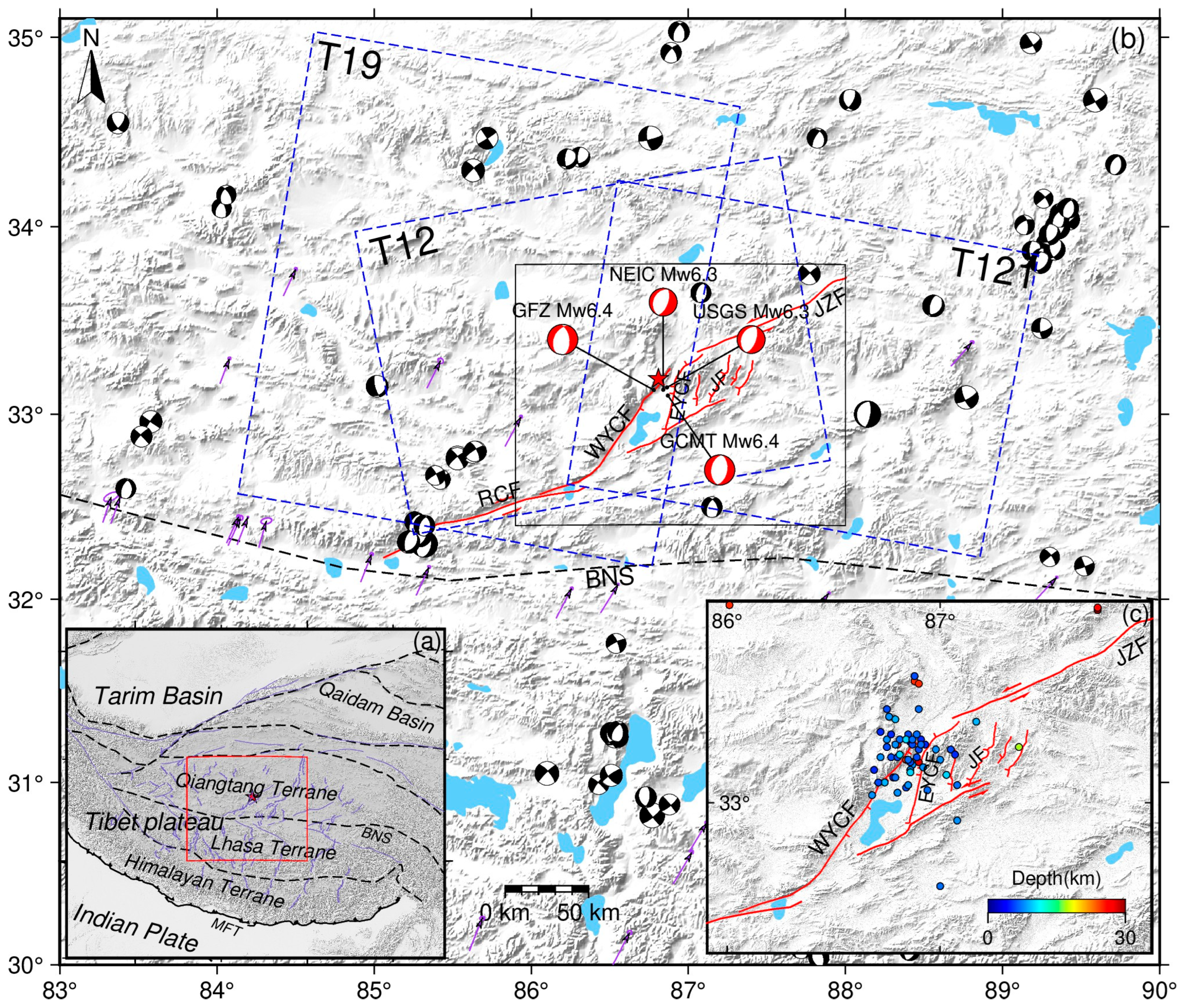
1. Introduction
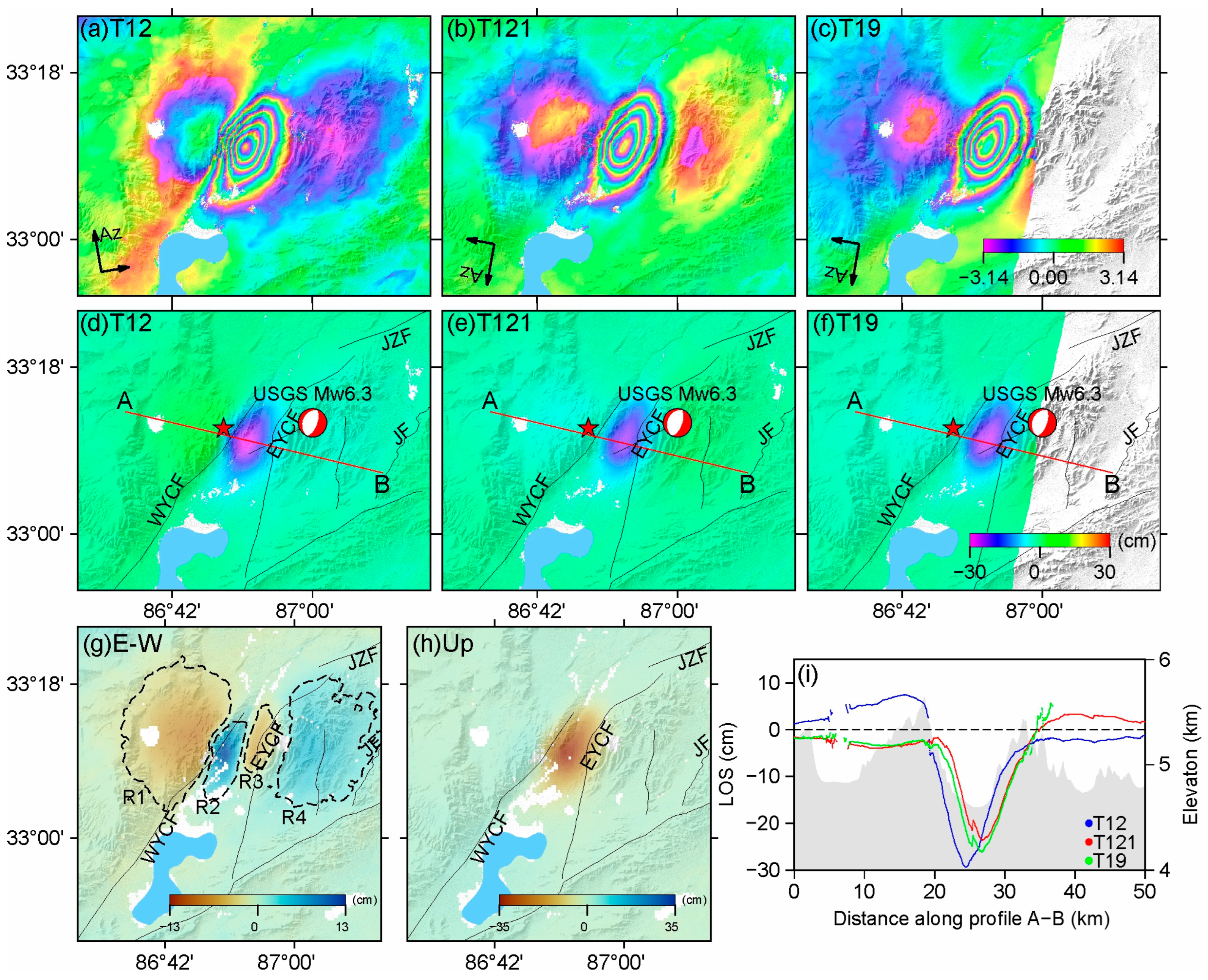
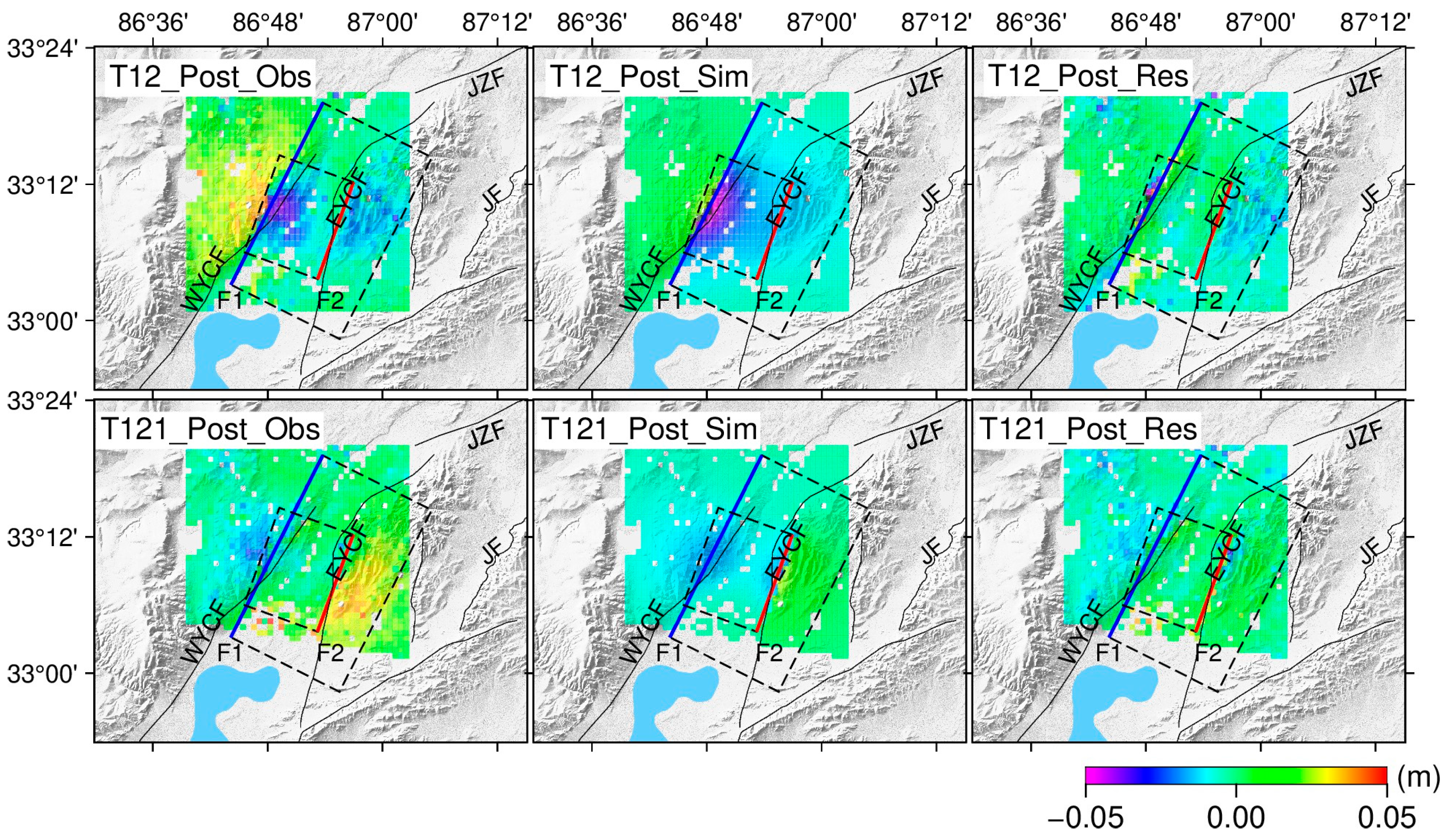
2. InSAR Data and Processing
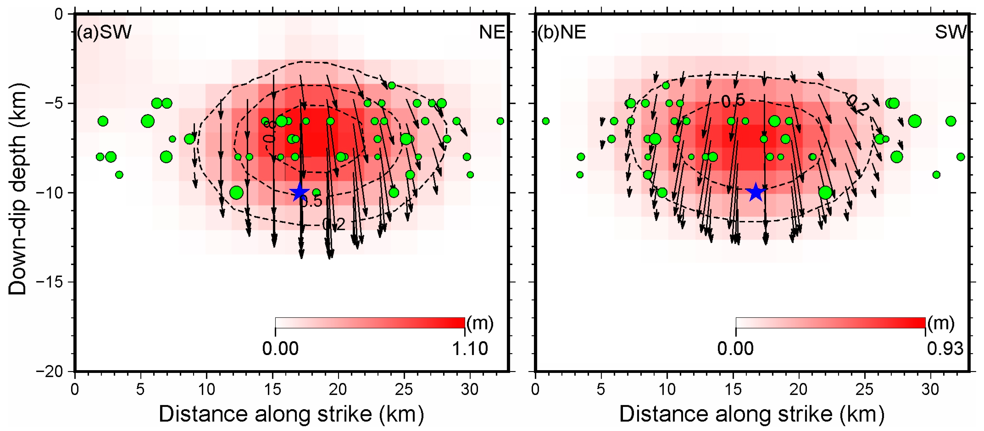
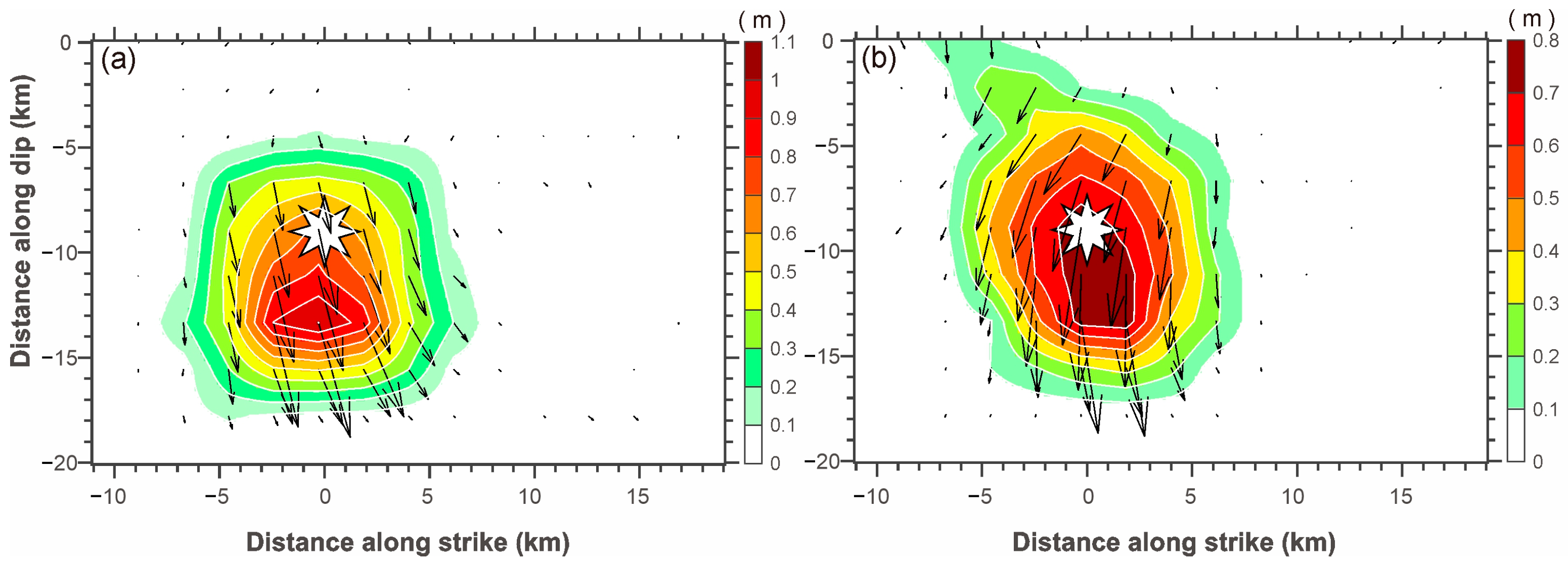
3. Coseismic Slip Distribution Inversion
3.1. InSAR Coseismic Slip Distribution Inversion
3.2. Teleseismic Waveform Data Inversion
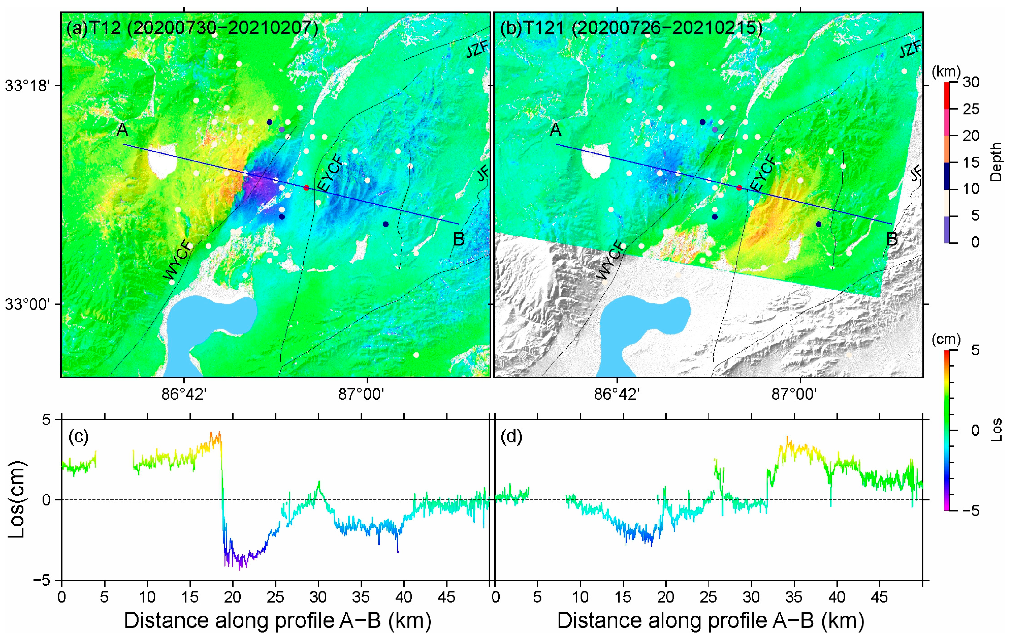
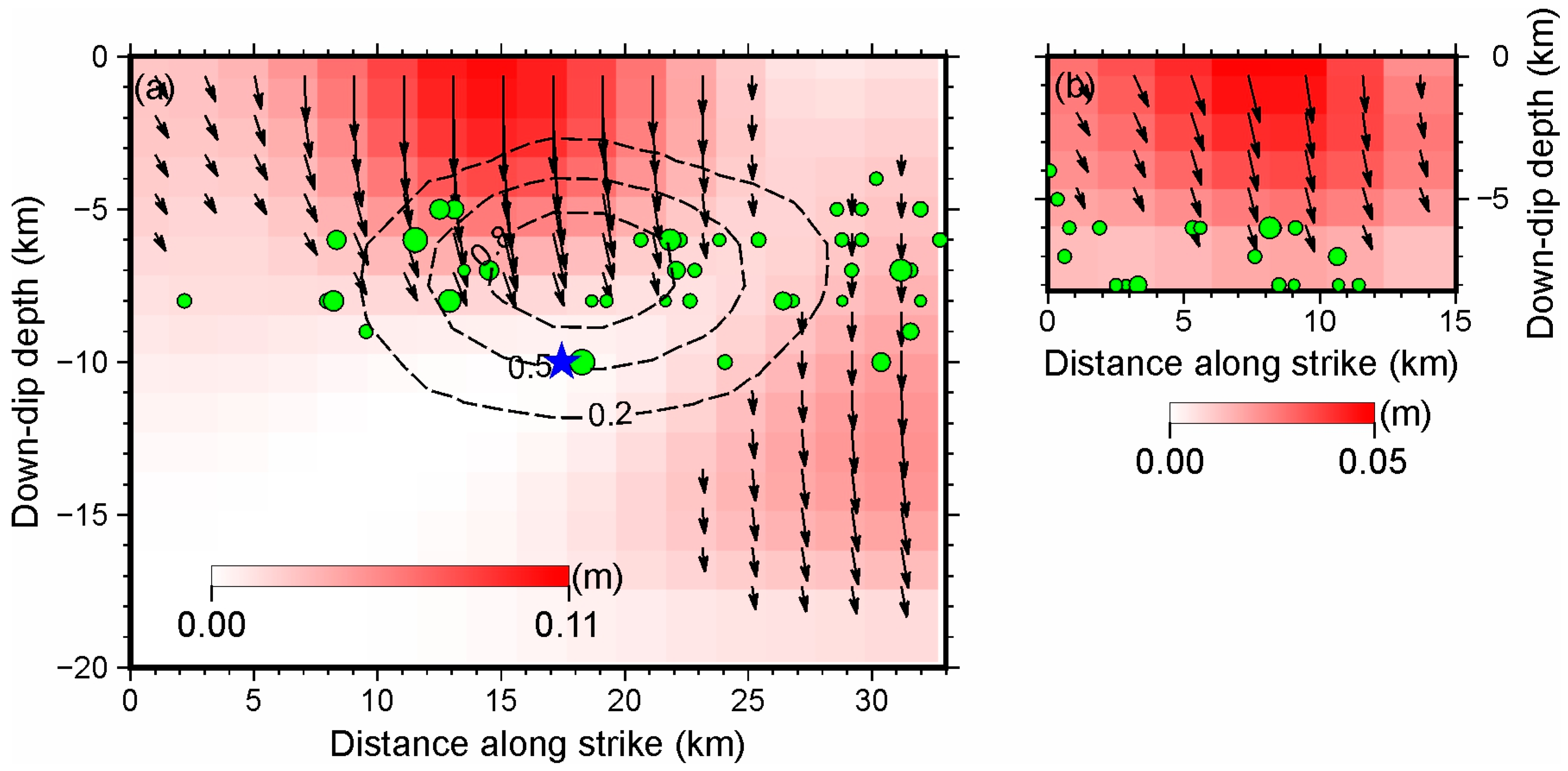
4. Afterslip Model
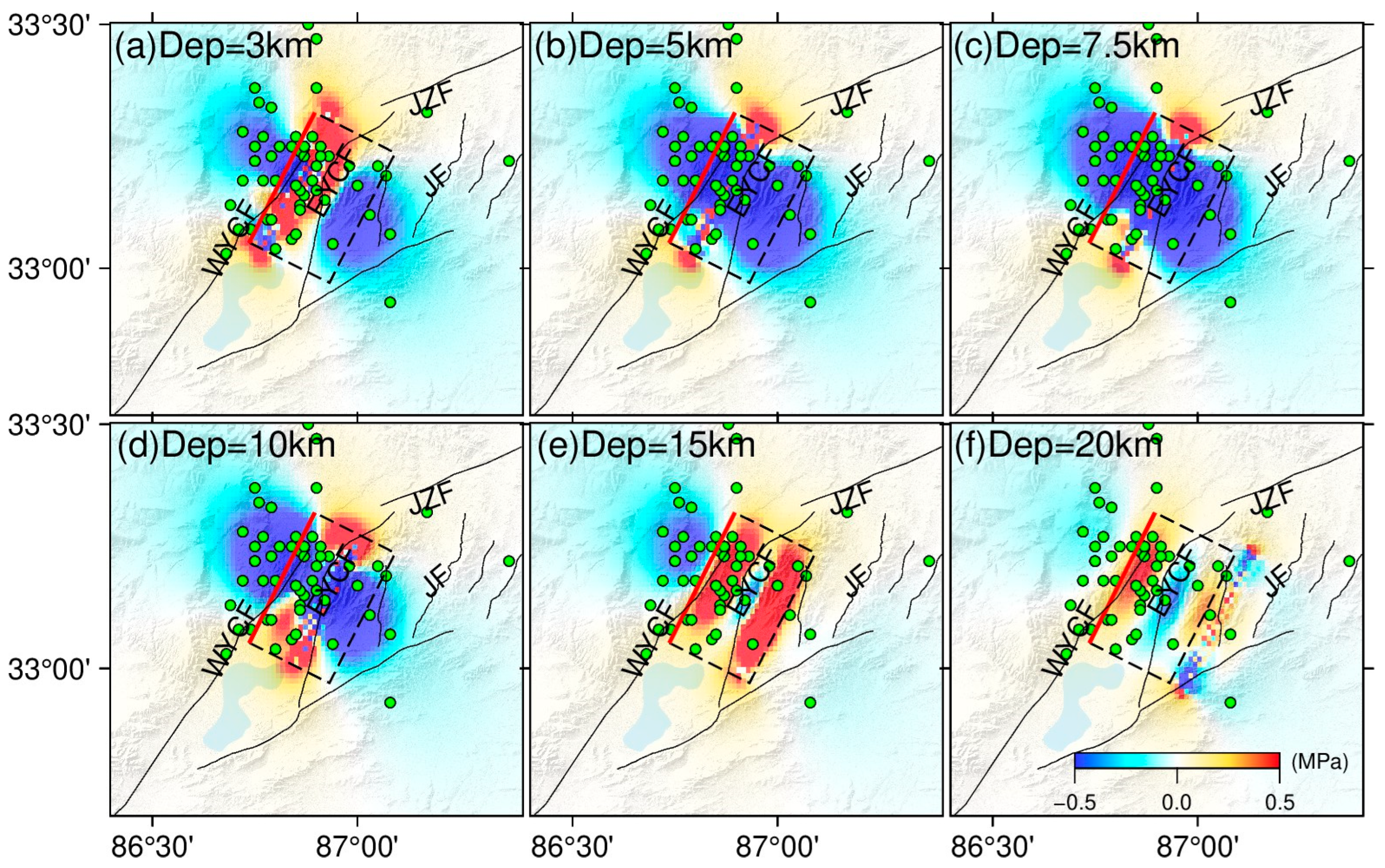
5. Discussion
5.1. The 2020 Nima Earthquake Fault Geometry
5.2. Coseismic Slip Distribution and Afterslip
5.3. Potential Hazards in the 2020 Nima Earthquake Source Area
6. Conclusions
Supplementary Materials
Author Contributions
Funding
Data Availability Statement
Acknowledgments
Conflicts of Interest
References
- Armijo, R.; Tapponnier, P.; Mercier, J.; Han, T.L. Quaternary extension in southern Tibet: Field observations and tectonic implications. J. Geophys. Res. Solid Earth 1986, 91, 13803–13872. [Google Scholar] [CrossRef]
- Tapponnier, P.; Zhiqin, X.; Roger, F.; Meyer, B.; Arnaud, N.; Wittlinger, G.; Jingsui, Y. Oblique stepwise rise and growth of the Tibet Plateau. Science 2001, 294, 1671–1677. [Google Scholar] [CrossRef] [PubMed]
- Yin, A. Mode of Cenozoic east-west extension in Tibet suggesting a common origin of rifts in Asia during the Indo-Asian collision. J. Geophys. Res. Solid Earth 2000, 105, 21745–21759. [Google Scholar] [CrossRef]
- Yin, A.; Taylor, M.H. Mechanics of V-shaped conjugate strike-slip faults and the corresponding continuum mode of continental deformation. Bulletin 2011, 123, 1798–1821. [Google Scholar] [CrossRef]
- Kapp, P.; Yin, A.; Manning, C.E.; Harrison, T.M.; Taylor, M.H.; Ding, L. Tectonic evolution of the early Mesozoic blueschist-bearing Qiangtang metamorphic belt, central Tibet. Tectonics 2003, 22, 17A. [Google Scholar] [CrossRef]
- Kapp, P.; Taylor, M.; Stockli, D.; Ding, L. Development of active low-angle normal fault systems during orogenic collapse: Insight from Tibet. Geology 2008, 36, 7–10. [Google Scholar] [CrossRef]
- Taylor, M.; Peltzer, G. Current slip rates on conjugate strike-slip faults in central Tibet using synthetic aperture radar interferometry. J. Geophys. Res. Solid Earth 2006, 111, B12402. [Google Scholar] [CrossRef]
- Taylor, M.; Yin, A.; Ryerson, F.J.; Kapp, P.; Ding, L. Conjugate strike-slip faulting along the Bangong-Nujiang suture zone accommodates coeval east-west extension and north-south shortening in the interior of the Tibetan Plateau. Tectonics 2003, 22, 18A. [Google Scholar] [CrossRef]
- Bie, L.; Ryder, I.; Nippress, S.E.; Bürgmann, R. Coseismic and post-seismic activity associated with the 2008 M w 6.3 Damxung earthquake, Tibet, constrained by InSAR. Geophys. J. Int. 2014, 196, 788–803. [Google Scholar] [CrossRef]
- Elliott, J.; Walters, R.; England, P.; Jackson, J.; Li, Z.; Parsons, B. Extension on the Tibetan plateau: Recent normal faulting measured by InSAR and body wave seismology. Geophys. J. Int. 2010, 183, 503–535. [Google Scholar] [CrossRef]
- Ryder, I.; Bürgmann, R.; Fielding, E. Static stress interactions in extensional earthquake sequences: An example from the South Lunggar Rift, Tibet. J. Geophys. Res. Solid Earth 2012, 117, B09405. [Google Scholar] [CrossRef]
- Ryder, I.; Bürgmann, R.; Sun, J. Tandem afterslip on connected fault planes following the 2008 Nima-Gaize (Tibet) earthquake. J. Geophys. Res. Solid Earth 2010, 115, B03404. [Google Scholar] [CrossRef]
- Sun, J.; Shen, Z.; Xu, X.; Bürgmann, R. Synthetic normal faulting of the 9 January 2008 Nima (Tibet) earthquake from conventional and along-track SAR interferometry. Geophys. Res. Lett. 2008, 35, L22308. [Google Scholar] [CrossRef]
- Wang, H.; Wright, T.J.; Liu-Zeng, J.; Peng, L. Strain rate distribution in south-central Tibet from two decades of InSAR and GPS. Geophys. Res. Lett. 2019, 46, 5170–5179. [Google Scholar] [CrossRef]
- Bai, L.; Chen, Z.; Wang, S. The 2025 Dingri MS6.8 earthquake in Xizang: Analysis of tectonic background and discussion of source characteristics. Rev. Geophys. Planet. Phys. 2025, 56, 258–263. [Google Scholar] [CrossRef]
- Wang, M.; Shen, Z.K. Present-day crustal deformation of continental China derived from GPS and its tectonic implications. J. Geophys. Res. Solid Earth 2020, 125, e2019JB018774. [Google Scholar] [CrossRef]
- Gao, H.; Liao, M.; Liang, X.; Feng, G.; Wang, G. Coseismic and postseismic fault kinematics of the July 22, 2020, Nima (Tibet) Ms6. 6 earthquake: Implications of the forming mechanism of the active N-S-trending grabens in Qiangtang, Tibet. Tectonics 2022, 41, e2021TC006949. [Google Scholar] [CrossRef]
- Liu, F.; Pan, J.; Li, H.; Sun, Z.; Liu, D.; Lu, H.; Zheng, Y.; Wang, S.; Bai, M.; Chevalier, M. Characteristics of quaternary activities along the Riganpei co fault and seismogenic structure of the July 23, 2020 Mw6. 4 Nima Earthquake, Central Tibet. Acta Geosci. Sin. 2021, 43, 173–188. [Google Scholar] [CrossRef]
- Hong, S.; Liu, M.; Zhou, X.; Meng, G.; Dong, Y. Afterslip on Conjugate Faults of the 2020 M w 6.3 Nima Earthquake in the Central Tibetan Plateau: Evidence from InSAR Measurements. Bull. Seismol. Soc. Am. 2023, 113, 2026–2040. [Google Scholar] [CrossRef]
- Liu, D.; Ferré, E.C.; Li, H.; Chou, Y.-M.; Wang, H.; Horng, C.-S.; Sun, Z.; Pan, J.; Chevalier, M.-L.; Zheng, Y. Magnetic evidence of seismic fluid processes along the East Yibug Chaka Fault, Tibet. Tectonophysics 2022, 838, 229500. [Google Scholar] [CrossRef]
- Li, K.; Li, Y.; Tapponnier, P.; Xu, X.; Li, D.; He, Z. Joint InSAR and field constraints on faulting during the Mw 6.4, July 23, 2020, Nima/Rongma earthquake in central Tibet. J. Geophys. Res. Solid Earth 2021, 126, e2021JB022212. [Google Scholar] [CrossRef]
- Yang, J.; Xu, C.; Wen, Y.; Xu, G. The July 2020 M w 6.3 Nima Earthquake, Central Tibet: A Shallow Normal-Faulting Event Rupturing in a Stepover Zone. Seismol. Soc. Am. 2022, 93, 45–55. [Google Scholar] [CrossRef]
- Zhang, M.; Li, Z.; Yu, C.; Liu, Z.; Zhang, X.; Wang, J.; Yang, J.; Han, B.; Peng, J. Co-and Postseismic Deformation of the 2020 Mw 6.3 Nima (Tibet, China) Earthquake Revealed by InSAR Observations. Remote Sens. 2022, 14, 5390. [Google Scholar] [CrossRef]
- ChengTao, L.; Qi, L.; Kai, T.; XiaoFei, L. Coseismic deformation characteristics of the 2020 Nima, Xizang M W 6.3 earthquake from Sentinel-1A/B InSAR data and rupture slip distribution. Chin. J. Geophys. 2021, 64, 2297–2310. [Google Scholar] [CrossRef]
- Gong, W.; Zhang, Y.; Li, T.; Wen, S.; Zhao, D.; Hou, L.; Shan, X. Multi-sensor geodetic observations and modeling of the 2017 Mw 6.3 Jinghe earthquake. Remote Sens. 2019, 11, 2157. [Google Scholar] [CrossRef]
- Rosen, P.A.; Gurrola, E.; Sacco, G.F.; Zebker, H. The InSAR scientific computing environment. In Proceedings of the EUSAR 2012, 9th European Conference on Synthetic Aperture Radar, Nuremberg, Germany, 23–26 April 2012; pp. 730–733. [Google Scholar]
- Farr, T.G.; Rosen, P.A.; Caro, E.; Crippen, R.; Duren, R.; Hensley, S.; Kobrick, M.; Paller, M.; Rodriguez, E.; Roth, L. The shuttle radar topography mission. Rev. Geophys. 2007, 45, RG2004. [Google Scholar] [CrossRef]
- Goldstein, R.M.; Werner, C.L. Radar interferogram filtering for geophysical applications. Geophys. Res. Lett. 1998, 25, 4035–4038. [Google Scholar] [CrossRef]
- Chen, C.W.; Zebker, H.A. Phase unwrapping for large SAR interferograms: Statistical segmentation and generalized network models. IEEE Trans. Geosci. Remote Sens. 2002, 40, 1709–1719. [Google Scholar] [CrossRef]
- Yu, C.; Li, Z.; Penna, N.T. Interferometric synthetic aperture radar atmospheric correction using a GPS-based iterative tropospheric decomposition model. Remote Sens. Environ. 2018, 204, 109–121. [Google Scholar] [CrossRef]
- Fialko, Y.; Simons, M.; Agnew, D. The complete (3-D) surface displacement field in the epicentral area of the 1999 Mw7. 1 Hector Mine earthquake, California, from space geodetic observations. Geophys. Res. Lett. 2001, 28, 3063–3066. [Google Scholar] [CrossRef]
- Fujiwara, S.; Nishimura, T.; Murakami, M.; Nakagawa, H.; Tobita, M.; Rosen, P.A. 2.5-D surface deformation of M6. 1 earthquake near Mt Iwate detected by SAR interferometry. Geophys. Res. Lett. 2000, 27, 2049–2052. [Google Scholar] [CrossRef]
- Mirzaee, S.; Amelung, F.; Fattahi, H. Non-linear phase linking using joined distributed and persistent scatterers. Comput. Geosci. 2023, 171, 105291. [Google Scholar] [CrossRef]
- Yunjun, Z.; Fattahi, H.; Amelung, F. Small baseline InSAR time series analysis: Unwrapping error correction and noise reduction. Comput. Geosci. 2019, 133, 104331. [Google Scholar] [CrossRef]
- Wang, R.; Diao, F.; Hoechner, A. SDM-A geodetic inversion code incorporating with layered crust structure and curved fault geometry. In Proceedings of the EGU General Assembly Conference Abstracts, Vienna, Austria, 7–12 April 2013; p. EGU2013-2411. [Google Scholar]
- Jónsson, S.; Zebker, H.; Segall, P.; Amelung, F. Fault slip distribution of the 1999 M w 7.1 Hector Mine, California, earthquake, estimated from satellite radar and GPS measurements. Bull. Seismol. Soc. Am. 2002, 92, 1377–1389. [Google Scholar] [CrossRef]
- Feng, W.; Li, Z.; Elliott, J.R.; Fukushima, Y.; Hoey, T.; Singleton, A.; Cook, R.; Xu, Z. The 2011 MW 6.8 Burma earthquake: Fault constraints provided by multiple SAR techniques. Geophys. J. Int. 2013, 195, 650–660. [Google Scholar] [CrossRef]
- Kennett, B.L.; Engdahl, E.; Buland, R. Constraints on seismic velocities in the Earth from traveltimes. Geophys. J. Int. 1995, 122, 108–124. [Google Scholar] [CrossRef]
- Wang, R. A simple orthonormalization method for stable and efficient computation of Green’s functions. Bull. Seismol. Soc. Am. 1999, 89, 733–741. [Google Scholar] [CrossRef]
- Zhang, Y.; Feng, W.; Chen, Y.; Xu, L.; Li, Z.; Forrest, D. The 2009 L’Aquila MW 6.3 earthquake: A new technique to locate the hypocentre in the joint inversion of earthquake rupture process. Geophys. J. Int. 2012, 191, 1417–1426. [Google Scholar] [CrossRef]
- Avouac, J.-P. From geodetic imaging of seismic and aseismic fault slip to dynamic modeling of the seismic cycle. Annu. Rev. Earth Planet. Sci. 2015, 43, 233–271. [Google Scholar] [CrossRef]
- Floyd, M.A.; Walters, R.J.; Elliott, J.R.; Funning, G.J.; Svarc, J.L.; Murray, J.R.; Hooper, A.J.; Larsen, Y.; Marinkovic, P.; Bürgmann, R. Spatial variations in fault friction related to lithology from rupture and afterslip of the 2014 South Napa, California, earthquake. Geophys. Res. Lett. 2016, 43, 6808–6816. [Google Scholar] [CrossRef]
- Ragon, T.; Sladen, A.; Bletery, Q.; Vergnolle, M.; Cavalié, O.; Avallone, A.; Balestra, J.; Delouis, B. Joint inversion of coseismic and early postseismic slip to optimize the information content in geodetic data: Application to the 2009 M w 6.3 L’Aquila earthquake, Central Italy. J. Geophys. Res. Solid Earth 2019, 124, 10522–10543. [Google Scholar] [CrossRef]
- D’agostino, N.; Cheloni, D.; Fornaro, G.; Giuliani, R.; Reale, D. Space-time distribution of afterslip following the 2009 L’Aquila earthquake. J. Geophys. Res. Solid Earth 2012, 117, B02402. [Google Scholar] [CrossRef]
- Fossen, H. Structural Geology; Cambridge University Press: Cambridge, UK, 2016. [Google Scholar]
- Jacques, E.; Kidane, T.; Tapponnier, P.; Manighetti, I.; Gaudemer, Y.; Meyer, B.; Ruegg, J.; Audin, L.; Armijo, R. Normal faulting during the August 1989 earthquakes in central Afar: Sequential triggering and propagation of rupture along the Dobi Graben. Bull. Seismol. Soc. Am. 2011, 101, 994–1023. [Google Scholar] [CrossRef]
- Nostro, C.; Chiaraluce, L.; Cocco, M.; Baumont, D.; Scotti, O. Coulomb stress changes caused by repeated normal faulting earthquakes during the 1997 Umbria-Marche (central Italy) seismic sequence. J. Geophys. Res. Solid Earth 2005, 110, B05S20. [Google Scholar] [CrossRef]
- Deng, J.; Sykes, L.R. Evolution of the stress field in southern California and triggering of moderate-size earthquakes: A 200-year perspective. J. Geophys. Res. Solid Earth 1997, 102, 9859–9886. [Google Scholar] [CrossRef]
- Harris, R.A. Introduction to Special Section: Stress Triggers, Stress Shadows, and Implications for Seismic Hazard; Wiley Online Library: Hoboken, NJ, USA, 1998; Volume 103, pp. 24347–24358. [Google Scholar]
- Luo, Y.; Ni, S.; Zeng, X.; Zheng, Y.; Chen, Q.; Chen, Y. A shallow aftershock sequence in the north-eastern end of the Wenchuan earthquake aftershock zone. Sci. China Earth Sci. 2010, 53, 1655–1664. [Google Scholar] [CrossRef]
- Wessel, P.; Smith, W.H.; Scharroo, R.; Luis, J.; Wobbe, F. Generic mapping tools: Improved version released. Eos Trans. Am. Geophys. Union 2013, 94, 409–410. [Google Scholar] [CrossRef]


| Models | Longitude (°) | Latitude (°) | Depth (km) | Strike (°) | Dip (°) | Rake (°) | Magnitude |
|---|---|---|---|---|---|---|---|
| USGS | 86.864 | 33.144 | 10 | 203/20 | 29/61 | −88/−94 | Mw 6.27 |
| GCMT | 86.86 | 33.09 | 17.3 | 187/12 | 14/46 | −94/−86 | Mw 6.40 |
| GFZ | 86.78 | 33.13 | 10 | 204/353 | 41/52 | −65/109 | Mw 6.40 |
| NEIC | 86.84 | 33.131 | 10 | 203/20 | 29/61 | −88/−91 | Mw 6.30 |
| CENC | 86.81 | 33.19 | 10 | 10/177 | 50/41 | −81/−100 | Ms 6.60 |
| This study | 86.90 | 33.17 | 7.5 | 26 | 43 | −87.28 | Mw 6.31 |
| Satellites | Reference Day | Secondary Day | Incidence (°) | Azimuth (°) | Tracks | Orbits |
|---|---|---|---|---|---|---|
| Sentinal 1A | 2020.7.18 | 2020.7.30 | 41.99 | −10.04 | 12 | Ascend |
| Sentinal 1A | 2020.7.14 | 2020.7.26 | 42.91 | −170.21 | 121 | Descend |
| Sentinal 1B | 2020.7.13 | 2020.7.25 | 34.63 | −169.34 | 19 | Descend |
| Models | Longitude (°) | Latitude (°) | Depth (km) | Strike (°) | Dip (°) | Rake (°) | Range (km) | Slip (m) | Mw |
|---|---|---|---|---|---|---|---|---|---|
| F1 | 86.90 | 33.17 | 7.50 | 26 | 43 | −87.28 | 3~13 | 1.10 | 6.31 |
| F2 | 86.87 | 33.18 | 7.05 | 203 | 40 | −95.54 | 3~13 | 0.93 | 6.26 |
| Models | Strike (°) | Dip (°) | Rake (°) | Slip (m) |
|---|---|---|---|---|
| F1 | 26 | 43 | −87.28 | 0.11 |
| F2 | 203 | 40 | −95.54 | 0.05 |
Disclaimer/Publisher’s Note: The statements, opinions and data contained in all publications are solely those of the individual author(s) and contributor(s) and not of MDPI and/or the editor(s). MDPI and/or the editor(s) disclaim responsibility for any injury to people or property resulting from any ideas, methods, instructions or products referred to in the content. |
© 2025 by the authors. Licensee MDPI, Basel, Switzerland. This article is an open access article distributed under the terms and conditions of the Creative Commons Attribution (CC BY) license (https://creativecommons.org/licenses/by/4.0/).
Share and Cite
Wang, S.; Bai, L.; Liu, C. Coseismic Rupture and Postseismic Afterslip of the 2020 Nima Mw 6.4 Earthquake. Remote Sens. 2025, 17, 1389. https://doi.org/10.3390/rs17081389
Wang S, Bai L, Liu C. Coseismic Rupture and Postseismic Afterslip of the 2020 Nima Mw 6.4 Earthquake. Remote Sensing. 2025; 17(8):1389. https://doi.org/10.3390/rs17081389
Chicago/Turabian StyleWang, Shaojun, Ling Bai, and Chaoya Liu. 2025. "Coseismic Rupture and Postseismic Afterslip of the 2020 Nima Mw 6.4 Earthquake" Remote Sensing 17, no. 8: 1389. https://doi.org/10.3390/rs17081389
APA StyleWang, S., Bai, L., & Liu, C. (2025). Coseismic Rupture and Postseismic Afterslip of the 2020 Nima Mw 6.4 Earthquake. Remote Sensing, 17(8), 1389. https://doi.org/10.3390/rs17081389