High-Precision Satellite Clock Offset Estimated by SRIF Based on Epoch-Wise Updated Orbit

Abstract

High-precision clock offset products directly affect the performance and reliability of precise point positioning (PPP) applications. Currently, real-time clock offset products offered by institutions such as the Centre national d’études spatiales (CNES) rely on ultra-rapid predicted orbits. However, these orbits have limited accuracy and exhibit jumps during updates, constraining the accuracy of real-time clock estimation. To address this issue, we propose an undifferenced ambiguity resolution (UD AR) technique for clock offset estimation based on epoch-wise updated orbits. Clock estimation experiments were performed using both predicted and epoch-wise updated orbits, with square root information filtering (SRIF) applied in three schemes: double-differenced (DD), UD, and float solutions. Compared with predicted orbits, epoch-wise updated orbits provided smoother sequences with higher accuracy, significantly improving clock offset estimation accuracy in all schemes. Moreover, the UD AR solution significantly enhanced clock offset estimation accuracy, and the high-precision epoch-wise updated orbit products increased the narrow-lane fixing rate of the UD solutions. The clock accuracies of BDS-3, Galileo, and GPS reached 0.032 ns, 0.023 ns, and 0.026 ns, respectively, representing improvements of 36%, 34%, and 41% compared with the float solutions and 41%, 30%, 26% compared with the UD solution based on 1 h predicted orbits. Finally, the positioning performance of the proposed method was validated via PPP using 25 stations, showing improvements of 50%, 48%, and 41% in the north, east, and up directions compared with CNES products. Therefore, by combining epoch-wise updated orbit products with the UD AR to improve clock accuracy, this method provides a new approach to generating high-precision clock products, significantly contributing to enhancing PPP services.

1. Introduction

Global Navigation Satellite System (GNSS) technology plays a vital role in high-precision positioning, navigation, and timing (PNT) applications [1]. As core elements of GNSS technology, real-time satellite clock offset products directly determine the quality of real-time applications such as precise point positioning (PPP) and PPP-RTK [2,3]. With the development of GNSS technology, the demand for real-time and high-precision applications has steadily increased, particularly in fields such as autonomous driving, precise agriculture, and geological hazard monitoring [4,5,6,7,8]. Consequently, real-time precise clock offset products have become a significant research focus in the GNSS field.

Currently, real-time clock offset products are primarily generated through two methods: prediction and estimation. Due to the relatively low precision of the prediction method, high-precision clock products predominantly rely on real-time clock estimation [9]. Over the past few years, numerous scholars have extensively researched satellite clock offset estimation. In terms of quality control, Fu et al. proposed an improved quality control algorithm based on the Sequential Least Squares (SLSQ) method, significantly enhancing clock offset accuracy [10]. Meanwhile, Bock et al. effectively eliminated outliers in observation data through post-residual analysis [11]. Regarding computational efficiency, studies have primarily focused on multi-threaded parallel processing, Kalman filtering, and square root information filtering (SRIF), all of which have demonstrated excellent performance in multi-system satellite clock offset estimation [12,13,14]. Furthermore, numerous studies have shown that ambiguity resolution (AR) techniques can substantially enhance the precision of satellite clock offset estimation [15,16,17,18], although fixing rates and computational efficiency require further enhancement.

In real-time clock estimation processing, satellite orbit products are typically considered known information, providing precise satellite positions at specific epochs [19]. As a result, the precision of real-time satellite orbit products directly determines the accuracy and reliability of real-time clock offset estimation [20]. Some institutes, such as the International GNSS Service (IGS), provide ultra-rapid predicted orbit products (e.g., IGU products), but these face challenges, such as discontinuities at update epochs and limited accuracy. These issues constrain further improvement in real-time clock estimation precision and, as a result, impact the performance of real-time PPP [21].

To address these challenges, this study proposes a clock estimation method based on epoch-wise estimated orbit products. Compared with ultra-rapid predicted orbit products, real-time epoch-wise estimated orbit products can effectively avoid discontinuities at update epochs and offer higher orbit accuracy, providing a foundation for high-precision real-time clock offset estimation. Notably, the Shanghai Astronomical Observatory (SHAO) has been releasing epoch-wise, updated, real-time estimated orbit products since November 2024, presenting a significant opportunity for advancing clock offset estimation research. Furthermore, to overcome the limitations of existing clock offset estimation methods, this study incorporates square root information filtering (SRIF) for parameter estimation and ambiguity resolution techniques to enhance the precision of real-time satellite clock offset estimation. The ultimate goal is to obtain high-precision products that support improvements in the service quality of real-time PPP.

This paper is organized as follows: Section 2 details the clock offset estimation model, ambiguity resolution technique, SRIF parameter estimation method, and data processing procedures. Then, the predicted and epoch-wise estimated orbits are analyzed in Section 3.1. Section 3.2 and Section 3.3 present an analysis of ambiguity resolution and a comparison of clock estimation based on different orbits. The results are then validated in Section 3.4 using kinematic PPP. Finally, Section 4 summarizes the conclusions.

2. Methods

This section introduces the mathematical models of clock estimation, undifferenced (UD) AR, double-differenced (DD), and real-time satellite clock estimation by SRIF. The sources of orbit data and our clock processing strategy are also illustrated.

2.1. Real-Time Clock Estimation Model

The ionospheric-free (IF) combination is an effective method for mitigating the impact of first-order ionospheric delays in observation data, commonly used in satellite clock offset estimation. For the dual-frequency IF combination observation from satellite ($s$) to receiver ($r$), the mathematical expression can be formulated as follows:

$$P_{r,IF}^s={\rho }_r^s+c\left({\overline{t}}_{r,IF}-{\overline{t}}_{IF}^s\right)+m_r^s{T}_r+{\epsilon }_{r,pc}^s$$

(1)

$$L_{r,IF}^s={\rho }_r^s+c\left({\overline{t}}_{r,IF}-{\overline{t}}_{IF}^s\right)+{\lambda }_{IF}{\overline{N}}_{r,IF}^s+m_r^s{T}_r+{\epsilon }_{r,lc}^s$$

(2)

where the $P_{r,IF}^s$ and $L_{r,IF}^s$ are the IF observations of the code and phase, respectively. ${\rho }_r^s$ is the distance between the satellite ($s$) to receiver ($r$). ${\overline{t}}_{r,IF}$ and ${\overline{t}}_{IF}^s$ represent clock offsets of the receiver and satellite after the IF combination, respectively, which include the uncalibrated hardware delays from the receiver $d_{r,IF}$ and satellite $d_{IF}^s$ [22]. These can be expressed as follows: ${\overline{t}}_{r,IF}=t_{r,IF}+d_{r,IF}$ and ${\overline{t}}_{IF}^s=t_{IF}^s+d_{IF}^s$. $m_r^s$ and $T_r$ are the mapping function and tropospheric zenith wet delay (ZWD). ${\lambda }_{IF}$ is the wavelength. ${\overline{N}}_{r,IF}^s$ is the re-parameterized phase ambiguity of the IF combination. ${\epsilon }_{r,pc}^s$ and ${\epsilon }_{r,lc}^s$ are the code and phase measurement noise, and $c$ denotes the speed of light.

2.2. Ambiguity Resolution

GNSS ambiguity resolution methods are primarily divided into DD and UD. Ambiguities lose integer characteristics after IF combinations and can be split into wide-lane (WL) and narrow-lane (NL). Since ambiguity absorbs the hardware delay at both the receiver and the satellite [22], it can be expressed as follows [16]:

$${\lambda }_{IF}.{\overline{N}}_{r,IF}^s={\displaystyle \frac{c{f}_2}{f_1^2-f_2^2}}{\overline{N}}_{r,WL}^s+{\displaystyle \frac{c}{f_1+f_2}}{\overline{N}}_{r,NL}^s$$

(3)

After the IF combination, the WL and NL ambiguities can be expressed as follows:

$${\overline{N}}_{r,WL}^s=N_{r,WL}^s+b_{r,WL}-b_{WL}^s$$

(4)

$${\overline{N}}_{r,NL}^s=N_{r,NL}^s+b_{r,NL}-b_{NL}^s$$

(5)

where $N_{r,WL}^s$ and $N_{r,NL}^s$ denote the integer WL and NL ambiguities. $b_{r,WL}$ and $b_{WL}^s$ are the WL uncalibrated phase delay (UPD) on the receiver and satellite sides, respectively. $b_{r,NL}$ and $b_{NL}^s$ are the NL UPD on the receiver and satellite sides, respectively.

The DD AR primarily eliminates the UPD of the satellite and receiver sides by differencing between two satellites, $s_1$ and $s_2$, and two receivers, $r_1$ and $r_2$. The specific principle is as follows:

$${∆\overline{N}}_{r_1{r}_2,WL}^{s_1{s}_2}=N_{r_1,WL}^{s_1}-N_{r_1,WL}^{s_2}-N_{r_2,WL}^{s_1}+N_{r_2,WL}^{s_2}$$

(6)

$$∆{\overline{N}}_{r_1{r}_2,NL}^{s_1{s}_2}=N_{r_1,NL}^{s_1}-N_{r_1,NL}^{s_2}-N_{r_2,NL}^{s_1}+N_{r_2,NL}^{s_2}$$

(7)

Substituting the above expression into Equation (3), the DD ambiguity can be expressed as follows:

$${\lambda }_{IF}.∆{\overline{N}}_{r_1{r}_2,IF}^{s_1{s}_2}={\displaystyle \frac{c{f}_2}{f_1^2-f_2^2}}{∆\overline{N}}_{r_1{r}_2,WL}^{s_1{s}_2}+{\displaystyle \frac{c}{f_1+f_2}}∆{\overline{N}}_{r_1{r}_2,NL}^{s_1{s}_2}$$

(8)

The MW (Melbourne–Wübbena) combination is commonly employed to compute float WL ambiguity. The UPD of the receiver and satellite sides can be eliminated by differencing between the satellites and the stations, enabling the determination of the DD WL ambiguity. If the fractional part of the rounded value of ${∆\overline{N}}_{r_1{r}_2,WL}^{s_1{s}_2}$ is smaller than the threshold, the ambiguity is successfully fixed. Then, DD NL ambiguity can be calculated using Equation (8), and the fractional component of the rounded value of the float DD NL ambiguity can be compared with the threshold. If the fractional part is smaller than the threshold, the ambiguity is successfully fixed; otherwise, it is not. Finally, the fixed and float DD ambiguities are combined to form the constraint equations. These are incorporated into the original equations for updating, improving the accuracy of the unknown parameters.

In terms of UD AR, the integer values of the UD WL ambiguities can be determined based on the MW combined observations [23,24], leaving the fractional parts, thus representing the WL UPD observation ${UPD}_{r,WL}^s$ as follows:

$${UPD}_{r,WL}^s=b_{r,WL}-b_{WL}^s+{\epsilon }_{WL}$$

(9)

where ${\epsilon }_{WL}$ is the noise of the observation. Assuming there are $rn$ stations capable of observing $sm$ satellites, the observation equation is given by the following:

$$\left[\begin{array}{c}{UPD}_{r1,WL}^{s1}\\ ⋮\\ {UPD}_{rn,WL}^{sm}\end{array}\right]=\left[\begin{array}{ccc}-1& \cdots & 0\\ ⋮& \ddots & ⋮\\ 0& \cdots & -1\end{array}\begin{array}{ccc}1& \cdots & 0\\ ⋮& \ddots & ⋮\\ 0& \cdots & 1\end{array}\right]\left[\begin{array}{c}{b}_{WL}^{s1}\\ ⋮\\ b_{rn,WL}\end{array}\right]$$

(10)

There is a linear relationship between the receiver clock and the satellite clocks, leading to a rank deficiency of 1 in Equation (10). Consequently, one satellite clock is chosen as the reference and set to 0. The least-square adjustment is then applied to estimate the UPD for the stations and satellites. Based on the WL UPD and IF ambiguities, the same processing procedure then can be employed to estimate the NL UPD.

If the WL and NL UPD products are obtained, the UD AR solution can be applied. Initially, the WL ambiguities are fixed. The criterion for determining if the WL ambiguities are fixed is based on whether the fractional part falls below the predefined threshold after accounting for the receiver and satellite UPD estimates. If this value is lower than the threshold, the ambiguities are fixed. In this study, the threshold for fixing UD WL ambiguity is 0.25 cycles. Subsequently, based on Equation (9), UD NL ambiguities can be fixed using the floating ambiguity variance and NL UPD. Once both the wide-lane and narrow-lane ambiguities are fixed, the IF ambiguity with integer characteristics can be resolved. Finally, the fixed ambiguities are combined with the float ambiguities to form a strong constraint added to the original equation for parameter updating, improving the precision of clock estimation.

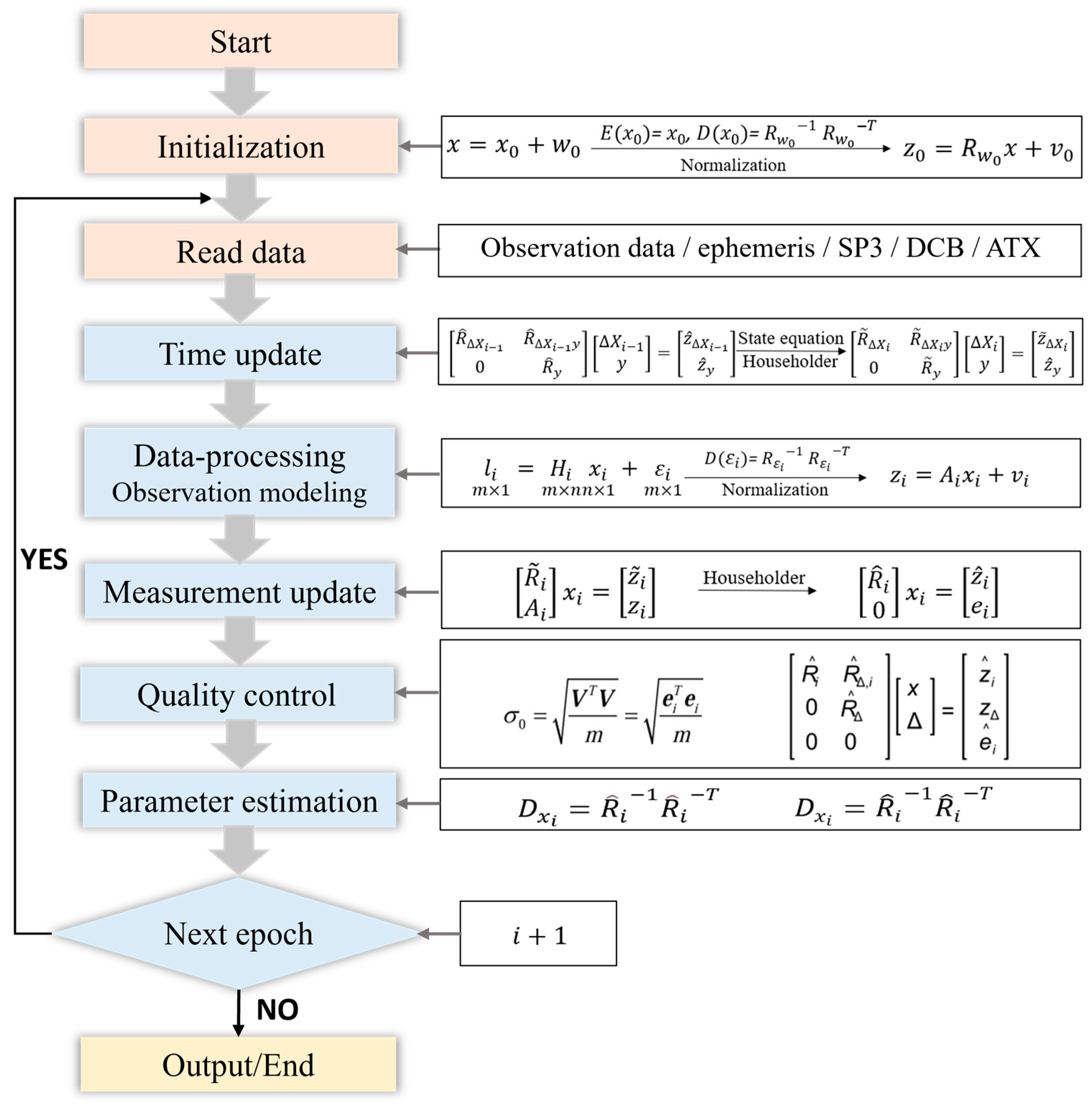
2.3. Real-Time Clock Estimation by SRIF

SRIF is a state estimation algorithm that enhances numerical stability and computational efficiency by decomposing the square root of the information matrix [25]. Assuming there are $m$ observations and $n$ unknown parameters $x$ at the epoch $i$, then the observation equation is given by the following:

$$\underset{m\times 1}{l_i}=\underset{m\times n}{H_i}\underset{n\times 1}{x_i}+\underset{m\times 1}{{\epsilon }_i}$$

(11)

where $l_i$ is the observation series, $H_i$ represents the design matrix, and ${\epsilon }_i$ indicates the measurement noise. The state parameters can be divided into time-varying parameters $∆X_i$ and deterministic parameters $y$. The state equation for the time-varying parameters is given by the following:

$$∆X_i={\mathsf{\Phi }}_{i,i-1}{∆X}_{i-1}+w_i$$

(12)

where ${\mathsf{\Phi }}_{i,i-1}$ represents the state transition matrix and $w_i$ denotes the processing noise with ${E(w}_i)=0,{D(w}_i)=D_{w_i}$. Given the initial values of the state parameters, the corresponding initial constraint equation is given by the following:

$$x=x_0+w_0$$

(13)

Since the SRIF requires that the noises must follow a normal distribution N (0,1), the aforementioned equations need to be standardized. The standardized equations are as follows:

$$\left\{\begin{array}{l}{z}_i=A_i{x}_i+v_i\\ R_{w_i}∆X_i={R_{w_i}\mathsf{\Phi }}_{i,i-1}{∆X}_{i-1}+{R_{w_i}w}_i\\ z_0=R_{w_0}x+v_0\end{array}\right.$$

(14)

where $z_i=R_{v_i}{l}_i$,$A_i=R_{v_i}{H}_i$, $v_i={R_{v_i}}^{-1}{\epsilon }_i$, $z_0=R_{w_0}{x}_0$, and $v_0=R_{w_0}{w}_0$.

In SRIF, the observation equations of the estimated parameters are as follows:

$$\left[\begin{array}{c}{R}_0\\ A\end{array}\right]x=\left[\begin{array}{c}{z}_0\\ z\end{array}\right]-\left[\begin{array}{c}{v}_0\\ v\end{array}\right]$$

(15)

The SRIF estimates the parameters epoch by epoch, and its time update relies on the information and parameter states from the previous epoch. The above equation can be expressed after the measurement update:

$$\left[\begin{array}{cc}{\hat{R}}_{{∆X}_{i-1}}& {\hat{R}}_{{∆X}_{i-1}y}\\ 0& {\hat{R}}_y\end{array}\right]\left[\begin{array}{c}{∆X}_{i-1}\\ y\end{array}\right]=\left[\begin{array}{c}{\hat{z}}_{{∆X}_{i-1}}\\ {\hat{z}}_y\end{array}\right]$$

(16)

Combining the state equation, the matrix after the time update is given by the following expression:

$$\left[\begin{array}{ccc}{{-R}_{w_i}\mathsf{\Phi }}_{i,i-1}& R_{w_i}& 0\\ {\hat{R}}_{{∆X}_{i-1}}& 0& {\hat{R}}_{{∆X}_{i-1}y}\\ 0& 0& {\hat{R}}_y\end{array}\right]\left[\begin{array}{c}{∆X}_{i-1}\\ {∆X}_i\\ y\end{array}\right]=\left[\begin{array}{c}{\hat{z}}_{w_i}\\ {\hat{z}}_{{∆X}_{i-1}}\\ {\hat{z}}_y\end{array}\right]$$

(17)

After the Householder orthogonal transformation, the above equation can be converted into an upper triangular matrix of the following form [13]:

$$\left[\begin{array}{ccc}{\tilde{R}}_{{∆X}_{i-1}}& {\tilde{R}}_{{∆X}_{i-1}{∆X}_i}& 0\\ 0& {\tilde{R}}_{{∆X}_i}& {\tilde{R}}_{{∆X}_{i}y}\\ 0& 0& {\tilde{R}}_y\end{array}\right]\left[\begin{array}{c}{∆X}_{i-1}\\ {∆X}_i\\ y\end{array}\right]=\left[\begin{array}{c}{\tilde{z}}_{w_i}\\ {\tilde{z}}_{{∆X}_i}\\ {\tilde{z}}_y\end{array}\right]$$

(18)

From the above equation, it is evident that the parameter ${∆X}_{i-1}$ can be eliminated. Consequently, the state parameters can be predicted by this equation:

$$\left[\begin{array}{cc}{\tilde{R}}_{{∆X}_i}& {\tilde{R}}_{{∆X}_{i}y}\\ 0& {\tilde{R}}_y\end{array}\right]\left[\begin{array}{c}{∆X}_i\\ y\end{array}\right]=\left[\begin{array}{c}{\tilde{z}}_{{∆X}_i}\\ {\hat{z}}_y\end{array}\right]$$

(19)

Following the time update, the state parameters for the current epoch are integrated into the equation. This updated equation is then used as the initial input for the measurement update, which can be represented as follows:

$$\left[\begin{array}{c}{\tilde{R}}_i\\ A_i\end{array}\right]x_i=\left[\begin{array}{c}{\tilde{z}}_i\\ z_i\end{array}\right]$$

(20)

By reapplying the Householder orthogonal transformation and updating the observations with the residuals, the equation is transformed into the following:

$$\left[\begin{array}{c}{\hat{R}}_i\\ 0\end{array}\right]x_i=\left[\begin{array}{c}{\hat{z}}_i\\ e_i\end{array}\right]$$

(21)

During the real-time satellite clock estimation, the observation residuals and the variance of unit weight are obtained from the covariance matrix. The residuals are stored in vector ${\mathit{e}}_{\mathit{i}}$ and ${\mathit{e}}_{\mathit{i}}~N(0,I)$. The variance of unit weight is given by the following:

$${\sigma }_0=\sqrt{{\displaystyle \frac{V^{T}V}{m}}}=\sqrt{{\displaystyle \frac{{\mathit{e}}_{\mathit{i}}^{\mathit{T}}{\mathit{e}}_{\mathit{i}}}{m}}}$$

(22)

By employing hypothesis testing to detect and identify outliers [26,27,28], and through steps such as the Householder orthogonal transformation, the following equation can be derived [13]:

$$\left[\begin{array}{cc}{\hat{R}}_i& {\hat{R}}_{∆,i}\\ 0& {\hat{R}}_{∆}\\ 0& 0\end{array}\right]\left[\begin{array}{c}x\\ ∆\end{array}\right]=\left[\begin{array}{c}{\tilde{z}}_i\\ z_{∆}\\ {\hat{e}}_i\end{array}\right]$$

(23)

The final solutions for the estimated parameters and covariance matrix are as follows:

$$x_i={{\hat{R}}_i}^{-1}{\hat{z}}_i$$

(24)

$$D_{x_i}={{\hat{R}}_i}^{-1}{{\hat{R}}_i}^{-T}$$

(25)

The overall process of real-time clock estimation based on SRIF is shown in Figure 1, which provides the main steps and corresponding formulas.

2.4. Data Collection and Processing Strategy

To evaluate the precision of clock estimation and the effectiveness of ambiguity resolution based on different orbit products, epoch-wise updated and predicted orbit products were collected for the experiment. Epoch-wise updated orbits for 1–31 October 2024 (DOY 275–305), were estimated using the same processing strategy as the real-time orbits recorded by the SHAO. Since the ultra-rapid orbit from IGS is updated every 6 h and lacks BDS data, the predicted orbits were obtained from the Wuhan University IGS analysis center, which generates ultra-rapid predicted orbits that are updated every hour based on observations (https://igs.org/products/#orbits_clocks-2024.09.17, accessed on 21 February 2025). Three sets of predicted orbits were then integrated into daily files with update intervals of 1 h, 3 h, and 6 h. Specifically, these updated orbit products are constructed by extracting segments from each ultra-rapid file starting from its update time. The orbits and clocks are compared to the precise products of the CODE (Center for Orbit Determination in Europe), ensuring the reliability and accuracy of the experimental results.

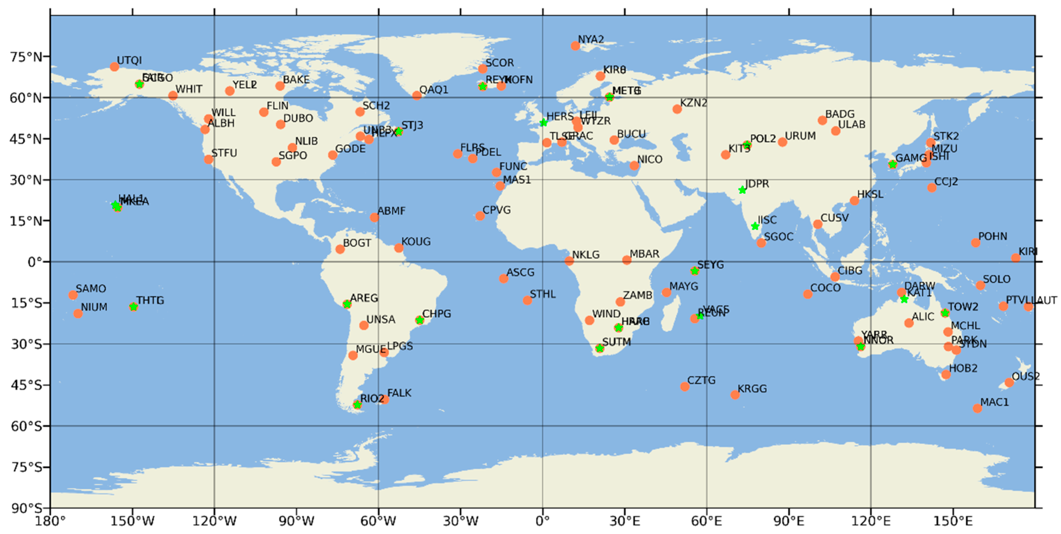
The station distribution of the clock estimation experiments is illustrated in Figure 2. The orange dots represent 100 stations estimating clocks, and the green stars represent 25 stations validating positioning results.

Table 1. Clock Offset Estimation Strategy.

Item	Strategy
Software	Modified PANDA
Stations	100 IGS/MGEX tracking stations [29,30]
Time interval	DOY 275–DOY 305, 2024
Observation	Undifferenced IF combination observations GPS: L1/L2, BDS-3: B1C/B2a, E: E1/E5a, R: G1/G2
Sampling interval	30 s
Cutoff angle	7°
Satellite antenna error	PCO and PCV corrections from the igs20.atx [31]
Receiver antenna error	PCO corrections from the igs20.atx [31]
Phase wind-up	Model correction [32]
Station coordinate	Fix to IGS weekly solution
Station displacement	Solid earth tide, pole tide and ocean tide: IERS Convention 2010 [33,34]
Satellite orbit and ERP	Real-time and predicted orbit products
Satellite and receiver clock	Estimated as white noise
ISB	Estimated as white noise
Estimator	SRIF
Troposphere delay	Saastamoinen model, GMF mapping function, piecewise constants [35,36]
Ambiguity	Estimated to be constant in the absence of cycle slips
Round-off criterion Differential code bias	0.25 cycles for WL, 0.15 cycles for NL CODE P1C1 bias product

outlines the specific strategy for real-time clock estimation. All experiments were conducted using the PANDA software. The clock estimation experiments for GPS, Galileo, and BDS-3 were conducted in three modes: UD, DD, and float. Due to the characteristics of the GLONASS, only the float solution was implemented.

3. Results

In this study, the accuracies of the predicted and epoch-wise updated orbit products were analyzed. Then, clock offset estimation experiments were conducted using SRIF based on these two products, and a discussion on the effects of UD and DD ambiguities fixing in clock offset estimation is presented. The clock offset accuracies were compared to precise clock products of the CODE. Finally, kinematic PPP was used for validation.

3.1. Analysis of Predicted and Estimated Satellite Orbit Products

To compare the differences between ultra-rapid predicted and real-time estimated satellite orbit products, precise orbits from the CODE were used as a reference to derive orbit residuals and accuracy. Taking BDS-3 as an example, the ultra-rapid orbit residuals at update intervals of 1 h, 3 h, and 6 h in the along (A), cross (C), and radial (R) directions are illustrated in Figure 3. Evidently, regardless of the update interval, significant jumps occurred in orbit residuals at each update epoch, indicating discontinuity in the residual sequences at these epochs. Additionally, the orbit accuracy of the 1 h update interval is superior to that of the 3 h and 6 h intervals, with the 6 h update exhibiting larger residual fluctuations and a wider distribution range. Out of all directions, the radial residuals are the smallest, while the along and cross residuals show larger variability.

Figure 4 shows the same day residuals of the real-time orbits estimated epoch by epoch for BDS-3. Compared with the predicted orbit residuals, these orbits demonstrate higher accuracy and better continuity. The satellites with larger residuals in the figure are C38, C39, and C40, which are IGSO satellites and exhibit lower orbit accuracy compared with MEO satellites. Excluding these three, the residuals of the remaining satellites in the A, C, and R directions fluctuate within 10 cm, indicating excellent overall performance.

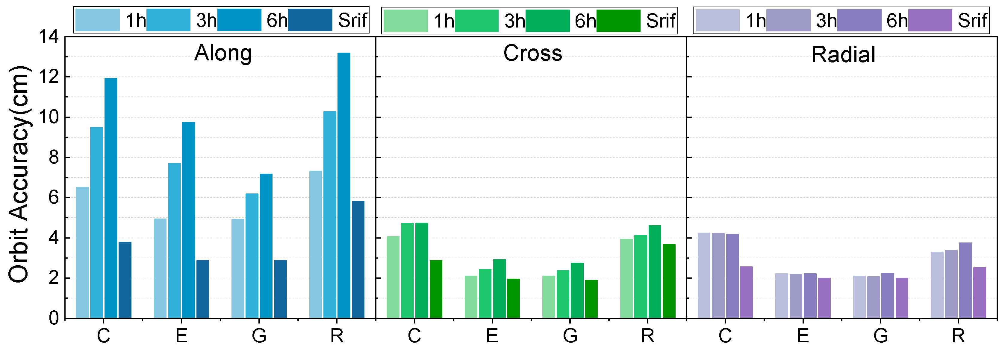
Figure 5 shows the average accuracy of the ultra-rapid predicted and epoch-wise updated orbits, where C, E, G, and R represent BDS-3, Galileo, GPS, and GLONASS, respectively. The labels 1 h, 3 h, 6 h, and SRIF represent predicted orbits with update frequencies of 1 h, 3 h, and 6 h, as well as epoch-wise updated orbits derived using SRIF. The accuracy of the along component is the worst, while the radial direction achieves the best accuracy, likely because a portion of radial errors are absorbed into the clock offset. For predicted orbits, the accuracies in the along and cross directions for a 1 h update frequency are significantly better than those with 3 h and 6 h update intervals, while the difference in the radial direction is minimal. The epoch-wise estimated orbit accuracy is clearly superior to that of the predicted orbit, with a particularly notable improvement in the along component. Additionally, the orbit accuracies of GPS and Galileo demonstrate superior performance, while BDS-3 and GLONASS exhibit comparable results. Overall, epoch-wise estimated orbits demonstrate a significant accuracy advantage, with the most noticeable improvement in the along direction.

The average 1D-RMS errors of the GNSS orbits are summarized in

Table 2. The average 1D-RMS of different orbit products (Unit: cm).

Scheme	BDS-3	Galileo	GPS	GLONASS
1 h	5.23	3.41	3.43	5.28
3 h	6.75	4.88	4.15	6.12
6 h	7.97	6.07	4.78	8.53
Epoch-wise	3.17	2.46	2.45	4.33

. Clearly, the orbit precision of Galileo and GPS is generally superior to those of BDS-3 and GLONASS. As the update frequency decreases, the accuracy of the predicted orbit becomes worse. Compared with predicted orbits, epoch-wise updated orbits demonstrate significant advantages in both accuracy and continuity.

3.2. Analysis of Ambiguity Resolution

In real-time clock estimation, orbit accuracy significantly impacts AR. In this section, UD, DD AR, and float solutions in clock estimation are applied to BDS-3, Galileo, and GPS based on predicted and epoch-wise updated orbit products. Then, the UD and DD ambiguity fixing rates of BDS-3, Galileo, and GPS are discussed.

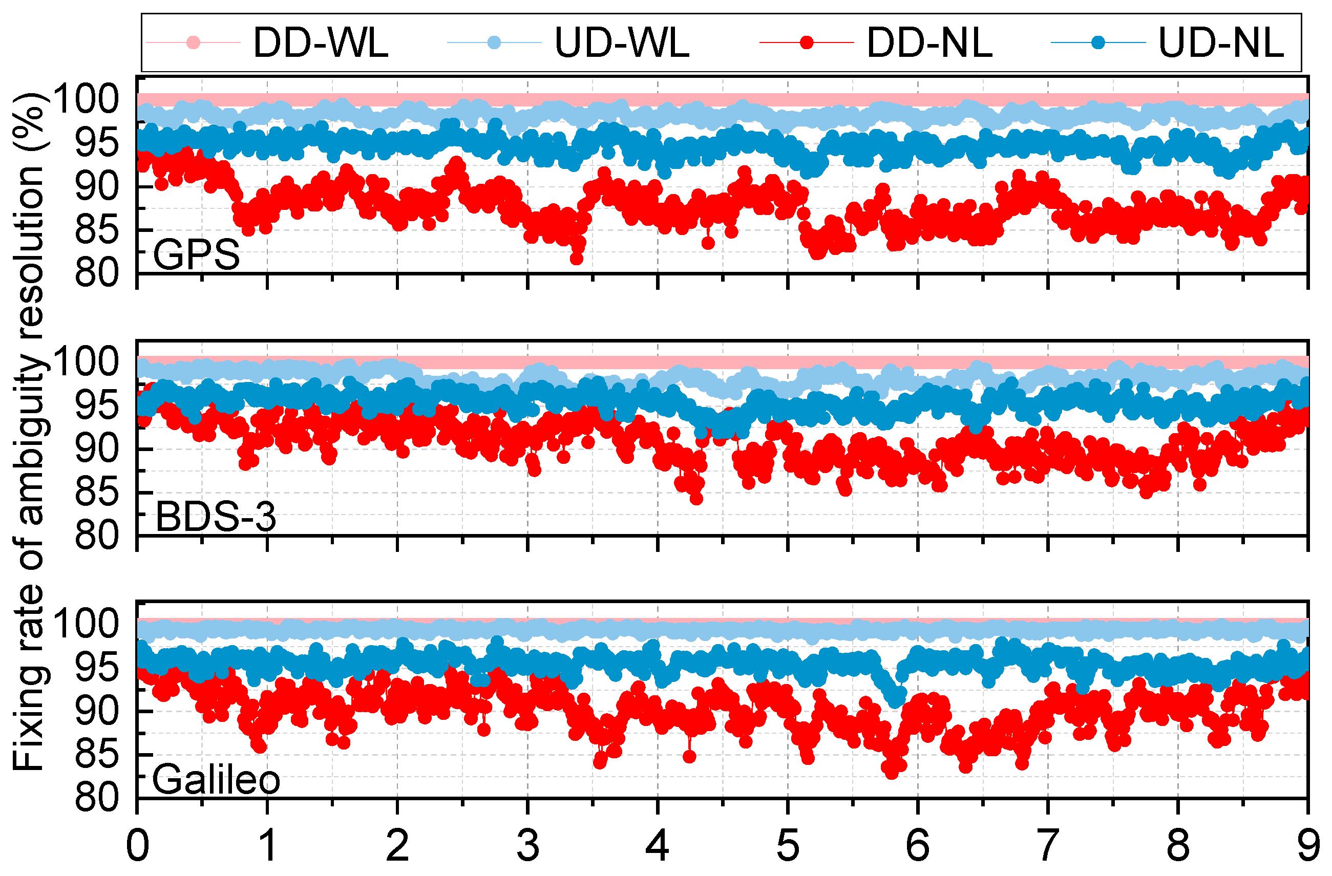
The WL and NL of the UD and DD ambiguity fixing percentages are displayed in Figure 6 based on epoch-wise updated orbits recorded over 10 days. The WL fixing rate of DD is 100% for all systems, while the NL fixing rate significantly decreases. This is because the observation data were preprocessed according to the elevation angle and quality control methods during the DD AR process. For UD, the WL fixing rate is nearly 99%, and the NL fixing rate slightly decreases, with fluctuations of around 95%. Compared with DD, the WL fixing rate is almost similar, while the NL fixing rate is notably high.

To explore the impact of different satellite orbits on the DD AR of clock offset estimation, Figure 7 presents DD ambiguity fixing rates in clock estimation based on 1 h, 3 h, and 6 h predicted orbit, as well as epoch-wise updated orbits (marked as SRIF). It can be seen that all the WL fixing rates for BDS-3, Galileo, and GPS based on different orbits reach 100%. Conversely, the average NL fixing rate for DD ambiguities ranges from approximately 84.7% to 90.1%. Epoch-wise updated orbits obviously outperform predicted orbits in NL fixing, and the NL fixing rate slightly decreases as the orbit update frequency decreases, indicating that orbit precision affects NL ambiguity fixing.

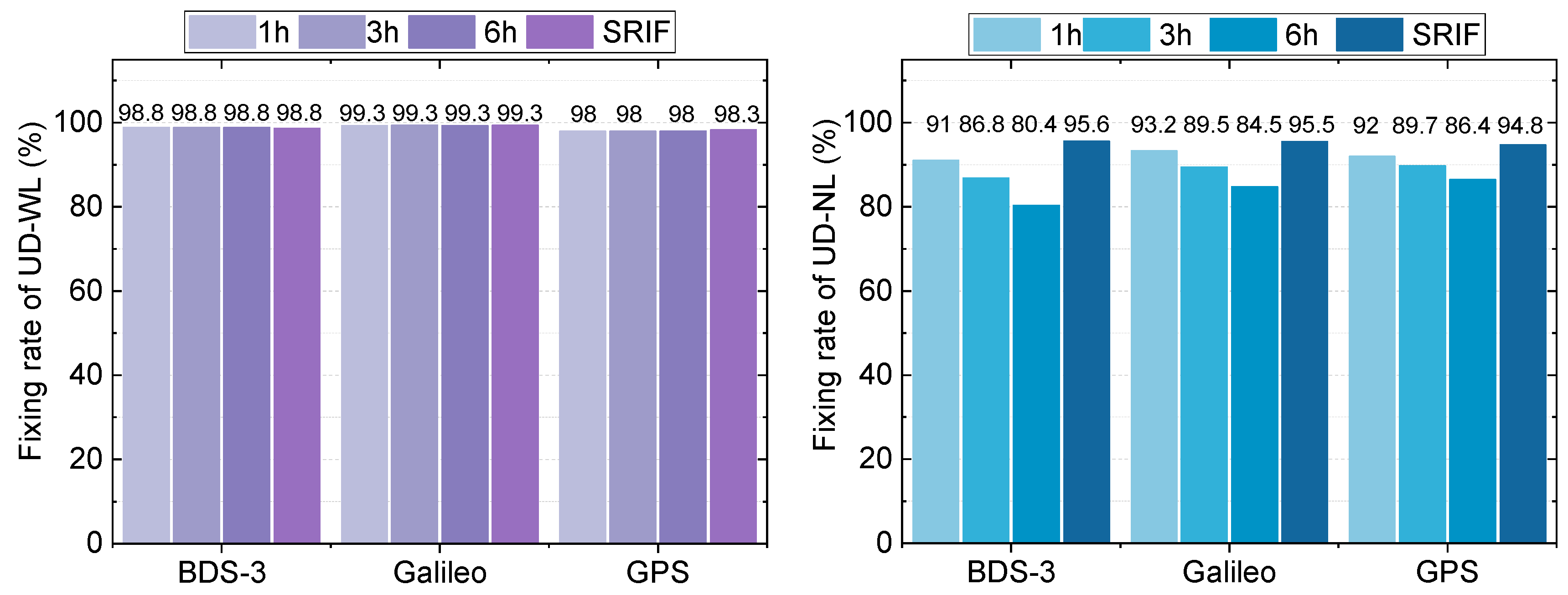
The UD ambiguity fixing rates of the predicted orbit are shown in Figure 8. The WL ambiguity fixing rates demonstrated excellent performance, with the rates for BDS-3, Galileo, and GPS all exceeding 98%. The results for the 1 h, 3 h, and 6 h predicted orbits, as well as for the epoch-wise updated orbits, show minimal variation. In terms of NL ambiguity fixing, predicted orbits with a 1 h update frequency exhibited significantly higher fixing rates than those of the 3 h and 6 h orbits. Furthermore, epoch-wise estimated orbits demonstrated a notable improvement over predicted orbits, particularly for BDS-3, where the NL fixing rate improved by 5%, 10%, and 19% compared with the 1 h, 3 h, and 6 h predicted orbits, respectively. Therefore, the quality and precision of orbit products have a remarkable impact on UD NL fixing, with higher-precision orbits leading to better fixing rates.

3.3. Comparison of Clock Estimation Results

Real-time clock offset estimation depends on accurate real-time orbit products as known information. Orbit products with high update frequency can promptly capture dynamic variations, thus reducing error accumulation. Therefore, the results for clock offset estimation based on predicted and epoch-wise estimated orbit products are compared below.

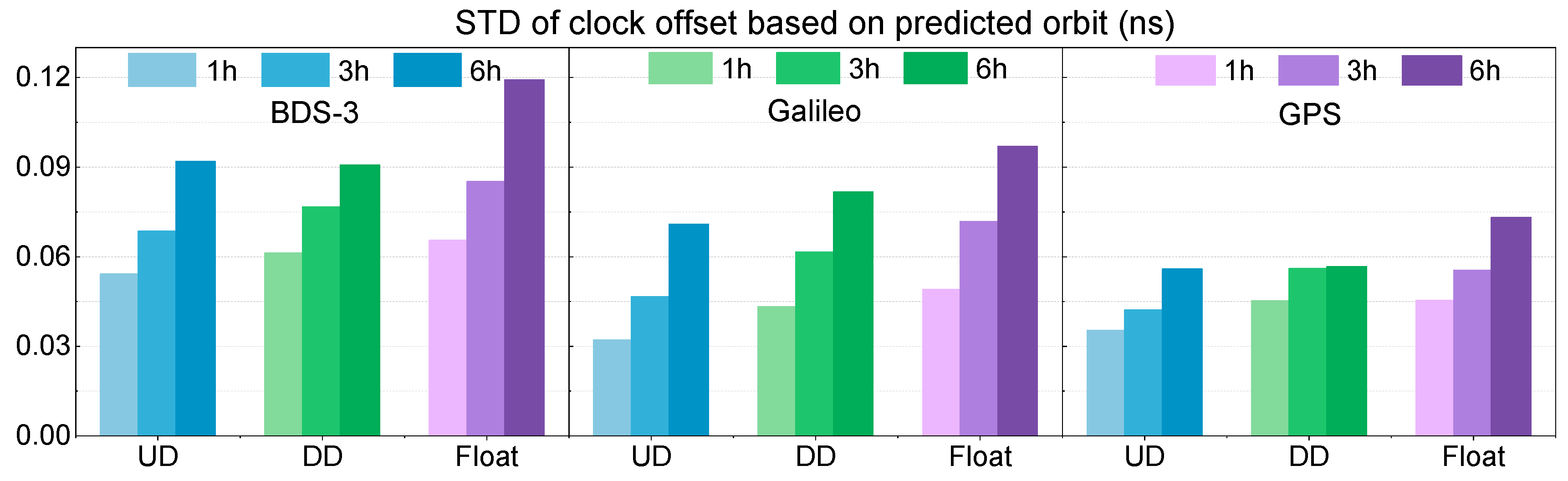
Figure 9 displays the average accuracy of satellite clocks estimated on basis of 1 h, 3 h, and 6 h predicted orbit products. The STDs of the clock offsets are calculated by first taking the mean of the single differences between all satellite clocks within the same GNSS system as a virtual reference and then computing the second differences relative to this mean. The standard deviation of these second differences is used as the clock STD. All results are better than 0.1 ns, except for the float solution with 6 h predicted orbits for BDS-3. The precision of satellite clock offsets significantly decreases as the predicted orbit update frequency reduces. Furthermore, the results for the DD and float solutions are slightly worse than those of the UD solution, indicating that the accuracy of satellite clock estimation can be improved by UD AR to some extent. It is notable that the clock offset accuracies of Galileo and GPS are slightly higher than those of BDS-3, which can be attributed to the more precise and stable ultra-rapid orbit products provided for Galileo and GPS. Therefore, both the accuracy and update frequency of satellite orbit products significantly impact the performance of real-time clock offset estimation.

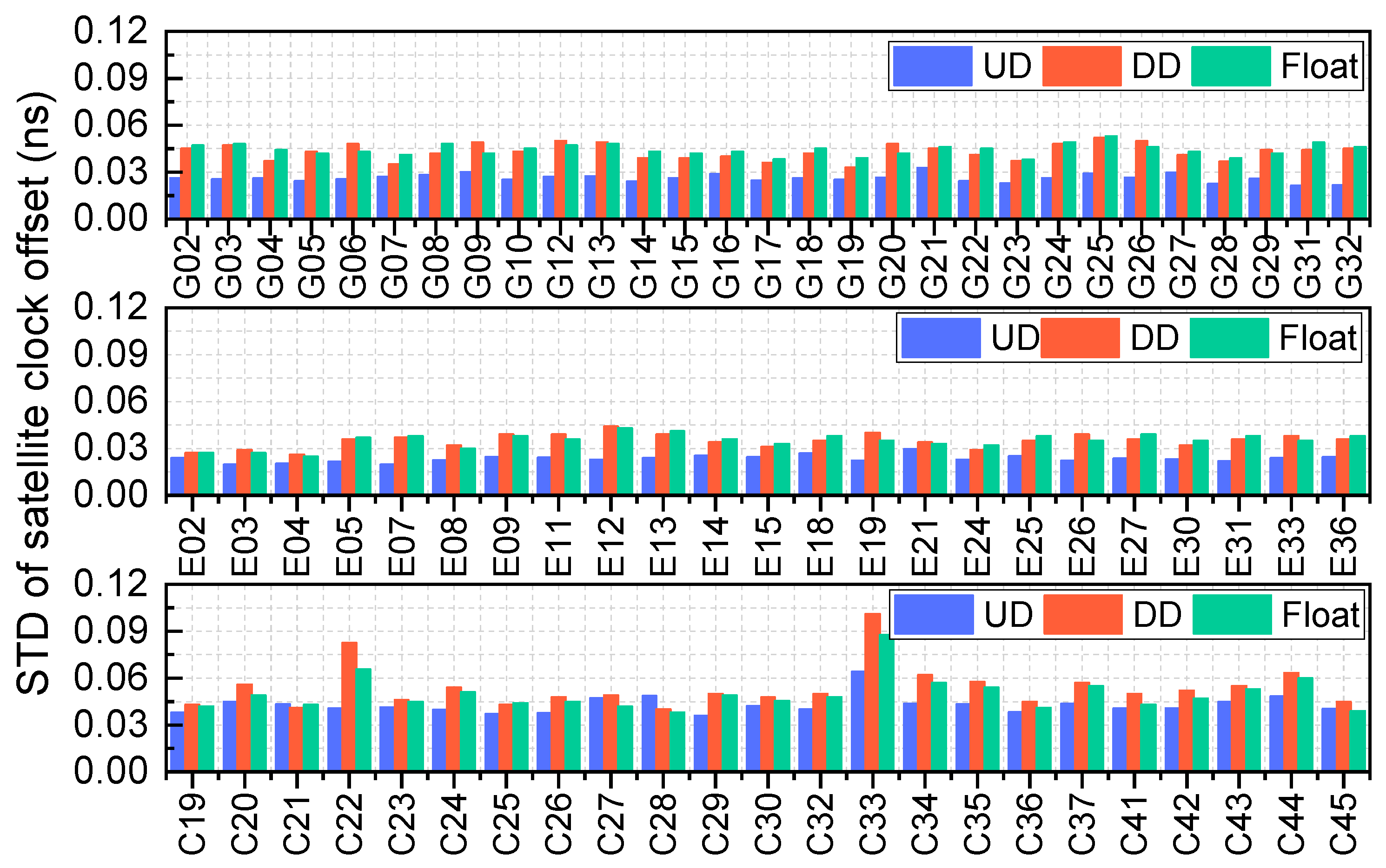
Figure 10 presents the clock estimation results for BDS-3, Galileo, and GPS with three schemes (UD, DD, and float), based on the epoch-wise estimated orbit, to further investigate the impact of orbit accuracy on clock offset estimation. The DD AR and float solutions are quite similar, and the UD solutions exhibit the best accuracy. Of the three systems, Galileo demonstrates the best performance, with a UD solution accuracy for all satellites within 0.03 ns. The GPS results are slightly better than those of BDS-3, with the most significant improvement observed after applying the UD AR. For BDS-3, the clock accuracy of the DD AR solution is worse than that of the float solution. Overall, the UD AR solution demonstrates a significant advantage in improving clock offset estimation accuracy.

From Figure 9 and Figure 10, it can be observed that both ambiguity resolution and high-quality orbit products significantly contribute to improving satellite clock offset estimation. Specifically, with float solutions, the epoch-wise updated orbits consistently outperform ultra-rapid orbit products in clock estimation accuracy across all solution types—float, DD, and UD. This highlights the advantage of the proposed orbits in real-time clock estimation. Moreover, regardless of the orbit used, the UD solution yields better clock estimation performance than the float and DD solutions. When using epoch-wise updated orbits, the NL fixing rate of UD is significantly higher, resulting in more accurate and stable clock estimates. This further demonstrates the effectiveness of the proposed method.

Table 3. The average accuracy of clock offset based on epoch-wise updated orbit (Unit: ns).

Scheme	BDS-3	Galileo	GPS
Float	0.050	0.035	0.044
DD	0.053	0.035	0.043
UD	0.032	0.023	0.026

shows the mean accuracy of clock offset estimation using SRIF based on estimated orbits. The DD solution clearly does not enhance the precision of real-time satellite clock offset estimation, as its results are nearly identical to those of the float solution. By contrast, the UD solutions provide the best performance. The BDS-3, Galileo, and GPS clock offset accuracies reach 0.032 ns, 0.023 ns, and 0.026 ns, respectively, representing improvements of 36%, 34%, and 41% compared with the float solution. In contrast to the results based on predicted orbits, all the UD, DD, and float solutions exhibit notable improvements. In conclusion, high-precision orbit products and UD AR significantly enhance real-time clock offset estimation.

3.4. PPP Validation

To further validate the performance of the optimal clock estimation method, kinematic PPP experiments with BDS-3, Galileo, and GPS were conducted using epoch-wise estimated orbit and the optimal clock products over 30 days. The PPP experiment involved 25 stations, as indicated in Figure 2. The IF combination with the same frequency as the clock offset estimation was used in the experiment. Furthermore, CNES real-time satellite orbit and clock products were used for comparison.

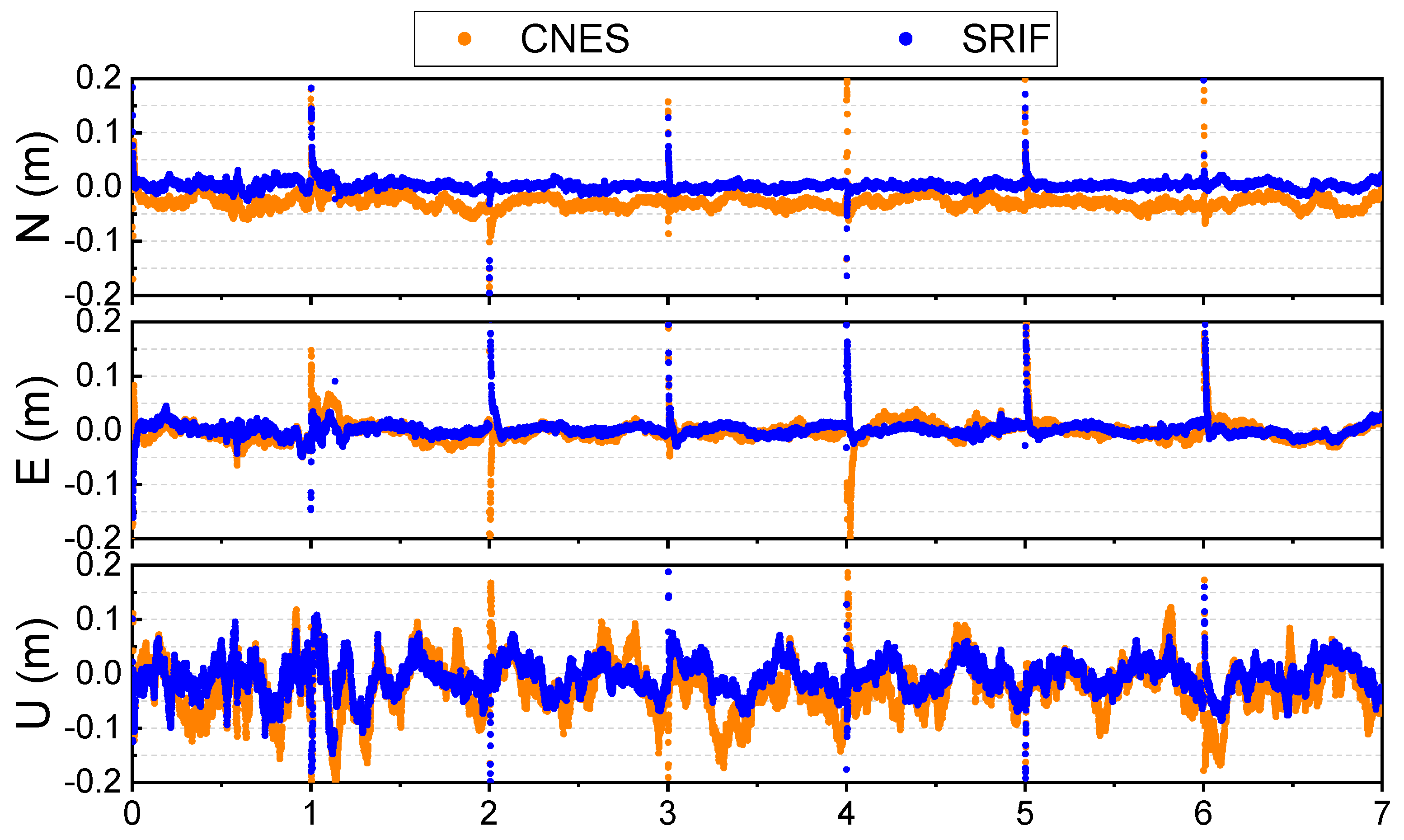
Positioning errors in the north (N), east (E), and up (U) directions for station TOW2 from DOY 287 to 293 are shown in Figure 11. The orange dots represent the positioning results using CNES real-time orbit and clock products, and the blue dots represent those of the estimated orbit and clock products combined with UD AR using SRIF. Both sets of results exhibit rapid convergence in all three directions, with errors in the N and E directions stabilizing after convergence. In comparison, the SRIF product provides more stable positioning results with higher accuracy in all three NEU directions, outperforming the CNES results.

Figure 12 presents the PPP positioning results for all stations using SRIF and CNES products. The red bars on the left represent the average convergence time in the N, E, and U directions, and the green bars on the right represent the accuracy in these directions. The convergence time of SRIF is slightly shorter than that of the CNES products for most stations in the N and U components. However, in the E component, some stations show a slower convergence when using SRIF products. Regarding positioning accuracy, the SRIF products outperform the CNES product in the N, E, and U components, demonstrating higher precision overall.

Table 4. Average positioning errors and convergence time for SRIF and CNES.

	N (cm)	E (cm)	U (cm)	Convergence Time (min)
SRIF	0.94	1.22	3.01	15.57
CNES	1.88	2.36	5.13	17.28

summarizes the average positioning precision and convergence time for the 25 stations. The PPP results demonstrate that the average convergence time using SRIF products is 15.57 min, comparable to the 17.28 min for the CNES products. Regarding positioning accuracy, the SRIF products achieve accuracies of 0.94 cm, 1.22 cm, and 3.01 cm in the N, E, and U directions, respectively, representing improvements of 50%, 48%, and 41% compared with CNES product. Consequently, the epoch-wise estimated orbit and UD AR satellite clock products using SRIF offer faster convergence and significantly enhance positioning accuracy for PPP.

4. Conclusions

Real-time clock offset products are among the core components of PPP services. Currently, real-time clock offset products provided by institutions such as the CNES rely on ultra-rapid predicted orbits. However, these predicted orbits have limited accuracy and discontinuous updates, which constrain the precision of real-time clock offset estimation. Therefore, this study proposes a UD AR clock offset estimation method implemented by SRIF based on real-time estimated orbits.

First, a comparison between the predicted orbits and the epoch-wise updated orbits highlighted the significant advantages of the latter in terms of both accuracy and continuity. Following this, three clock offset estimation schemes (UD, DD, and float solutions) were designed. The results show that the clock estimation accuracy and AR fixing rate can be significantly improved with high-precision epoch-wise updated orbits. In addition, the UD AR technique enhances clock offset estimation accuracy, while the DD AR does not significantly improve clock offset estimation. High-precision epoch-wise updated orbit products notably enhance the NL fixing rate of UD, substantially improving clock offset estimation accuracy. Specifically, the clock offset accuracies for BDS-3, Galileo, and GPS reach 0.032 ns, 0.023 ns, and 0.026 ns, respectively. Finally, the effectiveness of the proposed method was validated through PPP, and it was determined that this method outperforms real-time clock offset products based on predicted orbits of CNES. In conclusion, combining epoch-wise updated orbit products with the UD AR method can effectively improve the accuracy of real-time clock offset products, thereby enhancing the service quality of PPP.