Communication

Seismo-Traveling Ionospheric Disturbances from the 2024 Hualien Earthquake: Altitude-Dependent Propagation Insights

1
State Key Laboratory of Geohazard Prevention and Geoenvironment Protection (Chengdu University of Technology), Chengdu University of Technology, Chengdu 610059, China
2
School of Geophysics and Geomatics, China University of Geosciences, Wuhan 430074, China
3
Earthquake Agency of Xinjiang Uygur Autonomous Region, Urumqi 830011, China
4
Institute of Earthquake Forecasting, China Earthquake Administration, Beijing 100036, China
5
Institute of Applied Mechanics, School of Civil Engineering, Hefei University of Technology, Hefei 230009, China
6
College of Computer Science and Cyber Security, Chengdu University of Technology, Chengdu 610059, China
7
Qiaojia Seismological Bureau of Zhaotong City, Zhaotong 654600, China
*
Author to whom correspondence should be addressed.
Remote Sens. 2025, 17(7), 1241; https://doi.org/10.3390/rs17071241
Submission received: 6 February 2025 / Revised: 14 March 2025 / Accepted: 28 March 2025 / Published: 31 March 2025

Abstract

:
The propagation of seismo-traveling ionospheric disturbances (STIDs) is generally observed at one specific altitude layer. On 2 April 2024, a Mw 7.4 earthquake struck Hualien, which was the biggest earthquake since the 1999 Chi-Chi earthquake in the Taiwan region. In this study, a co-located vertical monitoring system combined with the observation of two horizontal layers in the ionosphere was utilized to study the STIDs associated with the Hualien earthquake. The vertical monitoring system can capture disturbances from the ground surface up to a height of ~350 km. In addition, changes in electric currents and the TEC (total electron content) at two horizontal layers, ~100 km and ~350 km, were monitored by permanent geomagnetic stations and a ground-based GNSS (global navigation satellite system) receivers network, respectively. The observations from this four-dimensional (4D) monitoring network show that the STIDs at a height of ~100 km associated with Rayleigh waves can propagate as far as 2000 km from the epicenter, while at an altitude of ~350 km, they can only propagate to about 1000 km. At an altitude of about 200 km, STIDs were also captured by a high-frequency Doppler sounder in a vertical monitoring system, which was consistent with the results in the geomagnetic field. The results from the 4D monitoring network suggest that the STIDs associated with Rayleigh waves exhibit different propagation ranges at various altitudes and prefer to propagate at low ionosphere layers. The vertical propagating waves typically only reach the bottom of the ionosphere and struggle to propagate to higher regions over long distances.

1. Introduction

Earthquakes can be monitored not only on the ground but can also affect the atmosphere and the ionosphere [1,2,3]. Ground vibrations due to earthquakes can trigger atmospheric waves [4,5,6]. The waves can propagate upward to the ionosphere, causing seismo-traveling ionospheric disturbances (STIDs, [7]). The STIDs can be detected in the vicinity of an epicenter due to vertical crustal displacements [8,9,10,11], and up to 6000–8000 km away from the epicenter when triggered by Rayleigh waves [12,13,14]. The atmospheric waves are recognized as acoustic waves whose frequencies are higher than ~3.3 mHz [5,15]. The exponential decrease in atmospheric density with the altitude leads to the growth of acoustic waves upon their upward propagation [16,17]. It usually takes ~8–14 min for acoustic waves to propagate from the surface to the ionosphere [15,18].
In the process of the upward propagation of acoustic waves due to earthquakes, STIDs can be detected from low to high altitudes by utilizing distinct parameters [19,20,21]. Seismic waves are firstly monitored by a seismometer to record the arrival time of surface ground vibrations [22]. The triggered acoustic waves then travel upward to an altitude of about 100 km, changing the electric currents [23], which in turn causes geomagnetic fluctuations [24]. Early studies observed earthquake-triggered geomagnetic fluctuations near the epicenter within several hundred kilometers [25,26]. Later, scientists expanded the focus to include more observations from near to far distances to investigate the horizontal propagations of the geomagnetic fluctuations. Hao et al. [27] observed far-field geomagnetic field fluctuations in Y (east–west) and Z (vertical) components about 2000–4000 km away from the epicenter of the 2011 Tohoku earthquake. They found that fluctuations with a duration of 2.1–3.3 min appeared about 8 min after the arrival of ground vibrations. Subsequent studies reported similar results and found that fluctuations had the speed of Rayleigh waves [28,29]. As the acoustic waves propagate up to an altitude of around 200 km, the ionospheric disturbances can be captured by a high-frequency (HF) Doppler sounder [1,30]. Chum et al. [31] monitored the STIDs on a horizontal plane of about 210–220 km after the Tohoku earthquake, utilizing five HF Doppler sounder observations. They found that disturbances appeared about 9 min after the arrival of ground vibrations, and the period of waves that can reach the disturbance height was longer than ~30 s. The GNSS (global navigation satellite system) can detect the total electron content (TEC), which is the electron density integrated along the ray path from a satellite to a receiver [32]. The electrons are concentrated at around the altitudes of the maximum ionospheric ionization. The ionosphere at these altitudes is usually assumed to be a thin spherical shell, which is at a height of approximately 350 km [15,33]. The GNSS TEC is widely studied for ionospheric disturbances caused by earthquakes [2,33,34,35]. Scientists have investigated the horizontal propagation of ionospheric disturbances at distinct altitudes [28,36]. In contrast, studying the propagation of ionospheric disturbances in the vertical profile is challenging because the observations are usually not co-located [37].
In 2021, an instrumental array within a 20 m × 20 m area was established in Leshan, Sichuan, China (103.91°E, 29.60°N) to monitor vibrations and perturbations in the lithosphere, atmosphere, and ionosphere at vertical profiles (the MVP-LAI system, [38]). The system comprises seismometers, a magnetometer, a ground-based GNSS receiver, and other instruments, which can monitor parameters ranging from the subsurface (−5 m) to the ionosphere (approximately 350 km). The signals from BeiDou geostationary satellites to GNSS receivers are used to analyze TEC variations because the ionospheric piercing points (IPPs) remain relatively fixed [34,39,40]. Additionally, a GNSS receiver was installed at the YADU substation (105.8°E, 31.8°N, Figure 1a) to continuously monitor TEC variations from BeiDou geostationary satellite C3, where the IPP was above the MVP-LAI system (Figure 1a,b; [41]). Recently, the MVP-LAI system implemented the installation of an HF Doppler sounder (Figure 1a,b) with a sounding frequency of 5 MHz, which can measure the electron density movements at an altitude of about 200 km (Figure 1b). Thus, the system is a truly co-located instrument array that can capture the vertical propagation of disturbances at distinct altitudes from the ground surface to the ionosphere.
On 2 April 2024, at 23:58:12 UT (Universal Time), a Mw 7.4 earthquake (121.60°E, 23.83°N) struck Hualien, on the eastern coast of the Taiwan region (http://earthquake.usgs.gov/earthquakes, accessed on 7 April 2024). The MVP-LAI system is located approximately 1860 km away from the epicenter (Figure 1a). We first collected multiple datasets from the MVP-LAI system to analyze the potential vertical propagation of STIDs associated with the earthquake. Then, we utilized the data from the network of permanent geomagnetic stations and ground-based GNSS receivers, which are located in the region between the epicenter and the MVP-LAI system, to discuss the horizontal propagations of the ionospheric disturbances at two altitude layers. Thus, the vertical and horizontal observations form a 4D monitoring network to capture and study the STIDs of the Hualien earthquake.

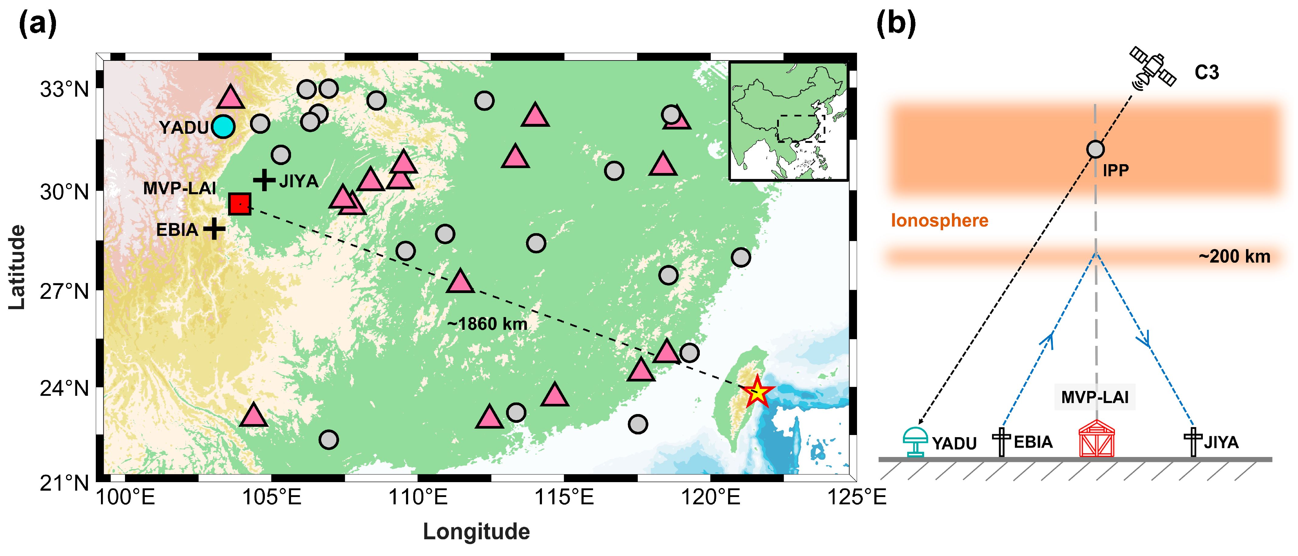
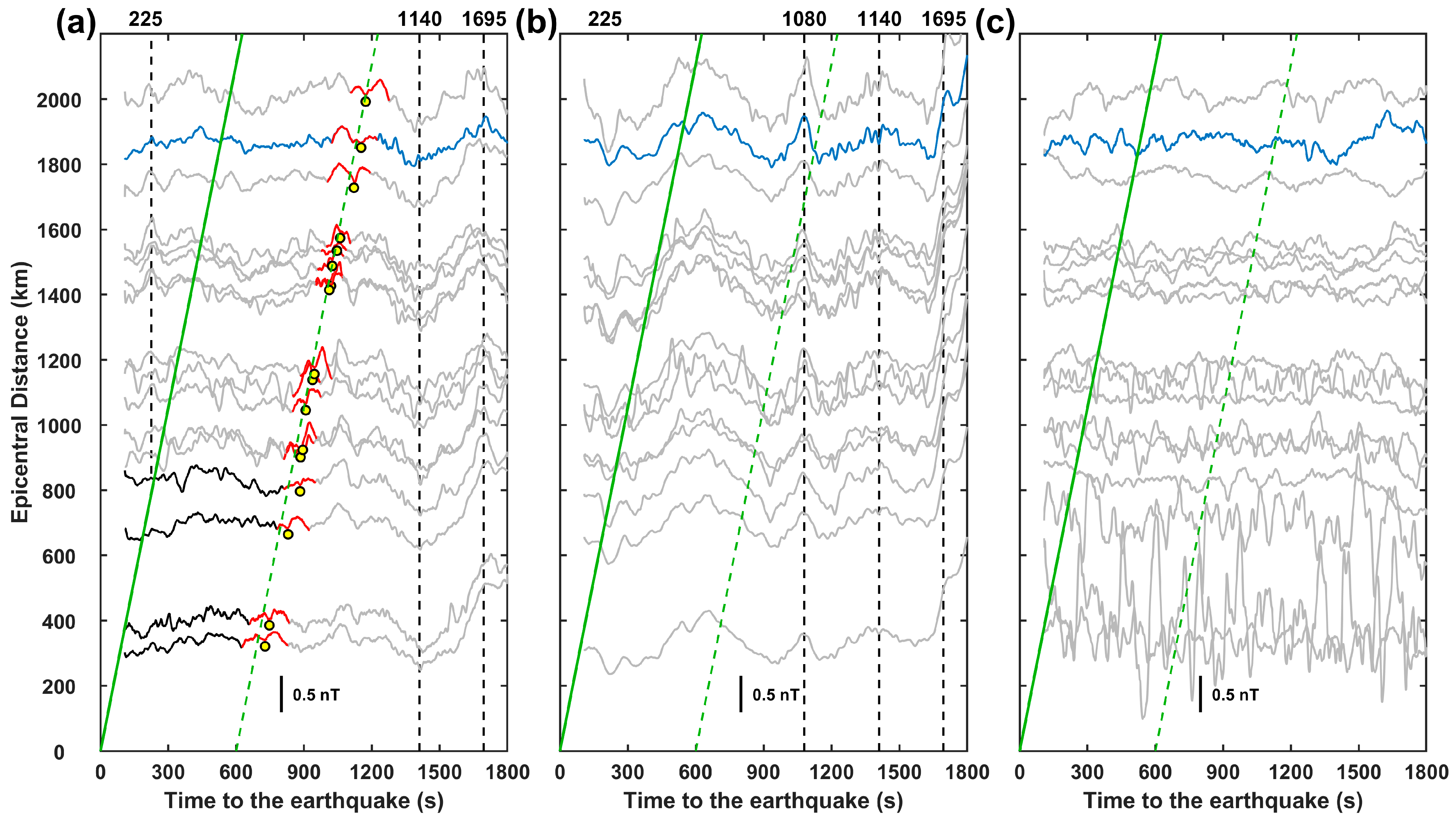
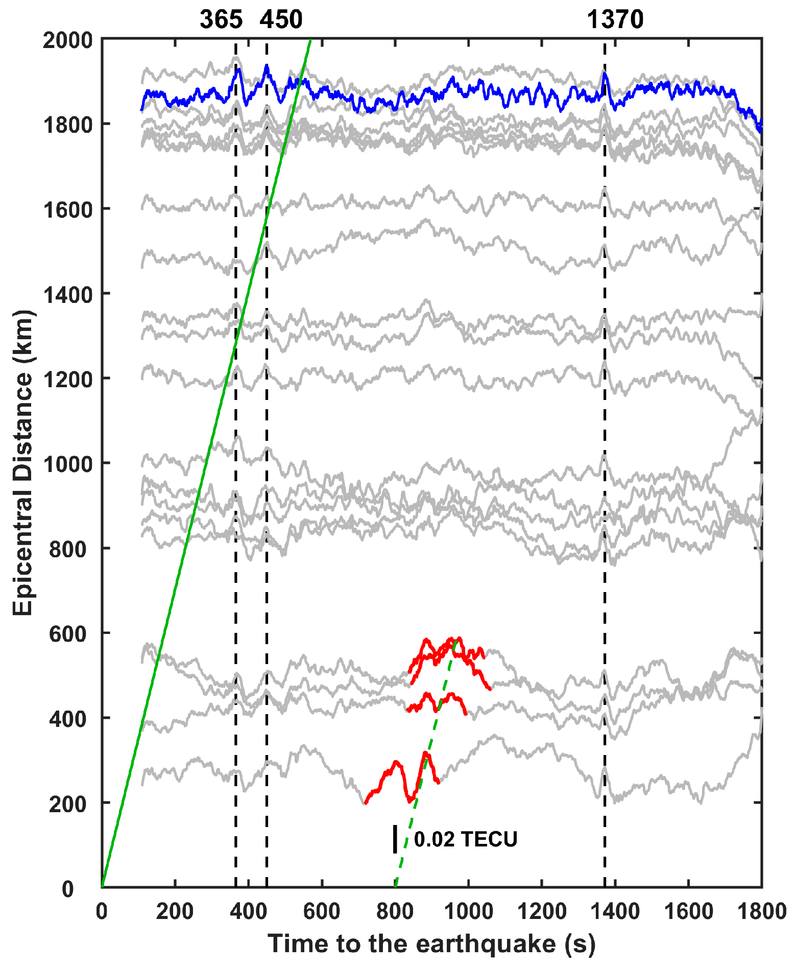
2. Observation and Interpretation

All data from the MVP-LAI system were promptly reviewed after the Hualien earthquake. Most parameters, such as temperature, air pressure, and surface vertical electric fields, did not exhibit obvious disturbances in the raw data following the earthquake, except for the Doppler shift and geomagnetic field. To analyze the potential disturbances triggered by the Hualien earthquake, we focus on the data regarding geomagnetic fields, Doppler shifts, and the TEC, which indicates disturbances at altitudes of approximately 100 km, 200 km, and 350 km in the vertical profile, respectively. Note that we focus on the variations of the TEC, not absolute values, so we ignore the instrumental bias terms in the process of calculating the TEC [42,43].
Figure 2a illustrates the raw data during the 200 s before and 1800 s after the earthquake, with 0 s representing the moment of the earthquake’s occurrence. The bottom panel shows the variations of vertical vibrations recorded by the seismometer. The arrival time of Rayleigh waves is approximately 530 s, and their average speed is around 3.51 km/s, considering the epicentral distance.
The most significant disturbances are found in the data from the Doppler sounder (i.e., Doppler shift (DS)) during approximately 1000–1200 s. We can see some small fluctuations in geomagnetic X and Y components in Figure 2a at approximately the same time, with the DS indicated by the shaded red areas. Geomagnetic field and TEC variations had linear backgrounds during the study period. This kind of linear background must be removed before analyzing disturbances. Previous studies reported that the periods of STIDs are typically within 300 s [15,44,45]. Here, all the raw data in Figure 2a are processed by subtracting a moving average with a time window of 300 s to mitigate the effect of longer period variations, and the residues are shown in Figure 2b. The DS exhibits disturbances with an amplitude of about 0.7 Hz, while the background variations are around 0. We found that the geomagnetic field exhibited fluctuations during the same temporal interval as DS disturbances, at approximately 1000–1200 s, as noted by the light red rectangle. These disturbances appear about 470–670 s (i.e., 7.8–11.2 min) after the arrival of Rayleigh waves. The time delays of 7.8–11.2 min between the disturbances and Rayleigh waves roughly agree with the propagation of acoustic waves from the ground to the ionosphere. The geomagnetic X component (MX) enhances from about 1020 s to 1200 s and reaches a local maximum value at 1065 s with an amplitude of about 0.27 nT. Its lowest value is at 1145 s. In terms of the Y component (MY), there are enhancements during 935–1145 s with an amplitude of ~0.73 nT, and it reaches its peak at 1080 s, which lags behind MX by 15 s. Compared to MX and MY, the fluctuations of the Z component (MZ) are not clear. There is no obvious perturbation in the TEC variations in Figure 2b.
To analyze the time–frequency characteristics of the disturbances in the DS and geomagnetic field described above, the short-time Fourier transform (STFT) is applied. Here, we employ a 600 s window with a 1 s step for STFT analysis. It is also utilized to investigate any potential perturbations associated with the earthquake with regard to the TEC. Figure 2c presents the spectrogram of the data in Figure 2a. The frequency bands of vertical vibrations mainly vary from ~20 mHz to 65 mHz. For the geomagnetic field, the fluctuations in MX intensify at approximately 3.3–10 mHz during a time span of about 1000–1200 s. MY shows a similar frequency range of enhancement, but the duration (i.e., ~900–1200 s) and pattern differ from those of MX. No amplitude enhancement is observed in MZ during the same time as MX and MY. In terms of DS, the disturbances cover the band of ~3.3–30 mHz. Regarding the variations in the TEC, there are still no signals accompanying or lagging behind the disturbances in DS.
To sum up, the disturbances in the geomagnetic field and DS are found at about 7.8 min after the arrival of Rayleigh waves in time series data, while there is no obvious perturbation in the TEC. In the frequency domain, the disturbances in the geomagnetic field and DS share the common frequency band of ~3.3–10 mHz simultaneously. The ionospheric disturbances might be related to the earthquake in the DS and geomagnetic field, but it is hard to distinguish them in the TEC, and this will be discussed later.

3. Discussion

The disturbances associated with earthquakes in the geomagnetic fields, DS, and GNSS TEC are mostly investigated separately [46,47]. The MVP-LAI system provides a unique opportunity to study the propagation of disturbances in the lithosphere, atmosphere, and ionosphere at different altitudes in a vertical profile [38,48,49]. Previous studies reported that the main periods of STIDs associated with Rayleigh waves in geomagnetic fields are approximately 3 min, and the time delay between magnetic fluctuations and Rayleigh waves is approximately 6–7 min [27,28,29,44]. In this study, through the MVP-LAI system, the period of geomagnetic fluctuations is about 1.7–5 min (i.e., ~3.3–10 mHz), and fluctuations lag behind the Rayleigh waves by ~7.8 min, which is a little longer compared with previous studies. This lag time is a function of the atmospheric density along the path and propagation angle of the acoustic waves [16]; therefore, the lag time can be variable in distinct atmospheric conditions and earthquake cases. The three components of the geomagnetic fields exhibit fluctuations at around 1000–1200 s after the earthquake (Figure 2b), but there are some time differences. The time of the local maximum in MY (i.e., 1080 s) lags behind that in MX (i.e., 1065 s) by 15 s, and the start time of the fluctuations in MY (i.e., 935 s) precedes that in MX (i.e., 1020 s) by 85 s. These indicate that there might be two or more effects causing the geomagnetic field fluctuations besides the earthquake. The vertical monitoring system can trace the waves from the surface to the ionosphere, while we still need to figure out how the waves propagate from the epicenter to the system. Investigation into the horizontal propagation of waves benefits the identification of disturbances associated with earthquakes.
Data from 16 permanent geomagnetic stations from the Geomagnetic Network of China (Figure 1a, noted by pink triangles) in the area between the epicenter and the MVP-LAI system are collected to track the horizontal propagation of fluctuations. Figure 3 presents the three-component geomagnetic field variations filtered by a 15–300 s bandpass at these permanent stations to mitigate the impact of high-frequency noise. The variations at these stations are arranged by epicentral distance from 0 to 2200 km. The blue lines indicate the data from the MVP-LAI system. The green solid line indicates the travel–time curve of Rayleigh waves with a speed of 3.51 km/s, referring to the seismic record of the MVP-LAI system.
In general, variations in the geomagnetic X component mainly correspond to solar effects, which usually change synchronously. In this study, at the near-field area within ~800 km of the epicenter, the variations initially exhibit inconsistent changes before ~600 s. Beyond 800 km, the variations show synchronous changes, such as a peak around 225 s, noted by the black dashed line, which is not observed in the near-field area. The inconsistent near-field geomagnetic fluctuations are attributed to local effects and may be caused by the earthquake (noted by black curves in Figure 3a). This indicates that other mechanisms might influence magnetic fields more quickly than Rayleigh waves. After around 600 s, we observe time-delayed fluctuations, noted by the “M” shape, with increasing epicentral distance, as indicated by the red curve in Figure 3a. Additionally, the duration of the “M” shape is approximately 200 s. Moreover, the fluctuations at the MVP-LAI system (i.e., blue curves) align with these time-delayed fluctuations. We find that the Rayleigh wave speed matches the propagation speed of the geomagnetic field fluctuations indicated by the green dashed line, which is shifted by 600 s. According to the green dashed line, the fluctuations begin to appear approximately 600 s (i.e., 10 min) after the earthquake near the epicenter (i.e., epicentral distance = 0). This corresponds to the time required for Rayleigh waves to trigger acoustic waves that subsequently propagate to the ionosphere [15,44]. This indicates that the geomagnetic field fluctuations in the X component, including those observed at the MVP-LAI system, are associated with Rayleigh waves. Therefore, it is inferred that the near-field magnetic field in variations in the X component before 600 s might result from local seismic-induced fluctuations affecting only regions within approximately 800 km. Subsequently, the Rayleigh wave-induced magnetic fluctuations can affect regions at least 2000 km away. Interestingly, following the fluctuations with the speed of Rayleigh waves, the geomagnetic fields at all stations exhibit synchronous changes, such as at 1410 s and 1695 s, as indicated by black dashed lines. The synchronous variations in geomagnetic fields recorded at different stations are mainly caused by solar activity, which is large-scale or even global-scale [50,51,52].
In Figure 3b, the Y component’s data show synchronous fluctuations, including at 1410 s and 1695 s, with the X component’s data at almost all stations, reflecting changes mainly caused by external fields (i.e., due to solar–terrestrial interactions). We have noted that the fluctuation times (i.e., ~935–1145 s) in MY have some discrepancies with MX (i.e., ~1020–1200 s) at the MVP-LAI system and might have different sources, as described in Figure 2. This point is demonstrated by Figure 3b, where the peaks at ~1080 s appear simultaneously at all stations and are not induced by the earthquake, as noted by the black dashed line. For the Z component, no variations can be found that are related to the earthquake. Nevertheless, the fluctuations associated with Rayleigh waves are detected in the X of the geomagnetic fields after the Hualien earthquake. We checked the Dst indices (https://wdc.kugi.kyoto-u.ac.jp/dst_provisional/202404/index.html accessed on 10 March 2025) and found that it was −1 nT during our study period. This indicates that the earthquake-related fluctuations in this study are not caused by external sources. Studies on magnetic disturbances after earthquakes are still rare, and recent works mainly reported the findings of the 2011 Tohoku M9 earthquake. In contrast, previous studies mainly found that the geomagnetic fluctuations induced by Rayleigh waves were significant in the Y and Z components [3,27,28,47]. The reasons for the differences in the fluctuated components of distinct earthquakes are not yet clear.
Compared to the fluctuations in geomagnetic fields, the disturbances in DS are more significant under a quiet background. The detected DS disturbances appeared with a frequency band of ~3.3–30 mHz, approximately 7.8 min after the arrival of Rayleigh waves. This roughly corresponds to the time required for the acoustic wave triggered by seismic waves to propagate from the ground to the lower ionosphere [46]. Previous studies found that DS disturbances related to earthquakes typically have a frequency lower than 30 mHz and lag 8–9 min behind the seismic waves [31,45], which is consistent with our results. Additionally, the observed frequency bands of the disturbances in DS align with the fact that it is reliable to detect acoustic waves with frequencies lower than 100 mHz at F2 region heights [5,12,53,54,55]. The disturbances in DS manifest simultaneously with the Rayleigh wave-triggered fluctuations in the MX components at the MVP-LAI system. This indicates that they are caused by the same source. From the single station, it is difficult to determine whether the source originates from ionospheric physical processes or the earthquake. However, time delays in geomagnetic fluctuations, consistent with the velocity of Rayleigh waves observed at multiple stations, indicate that the disturbances originate from the earthquake. Previous studies have claimed two mechanisms to explain how the Rayleigh waves cause geomagnetic field fluctuations. One is that Rayleigh waves could trigger acoustic waves propagating upward to the ionosphere, significantly modifying Hall and Pedersen conductivity at an altitude of about 105–110 km, which in turn affects the magnetic field [28,29,44]. Later, the acoustic waves continually propagate upward to perturbate higher layers of the ionosphere, which can be captured by the HF Doppler sounder [44]. The other mechanism is that acoustic waves triggered by Rayleigh waves directly propagate to the ionosphere at heights higher than 110 km to interact with electron-inducing ionosphere currents, synchronously causing geomagnetic fluctuations [47,56]. The synchronous variations in the geomagnetic field and Doppler shift in this study are possibly caused by the second mechanism. In other words, the Rayleigh waves trigger acoustic waves that propagate upward, disturbing the ionosphere at ~200 km, which then modulates the current, causing the magnetic field in the lower ionosphere.
In the lower ionosphere at an altitude of approximately 100–200 km, the disturbances associated with the Hualien earthquake are observed in the geomagnetic field and Doppler shift. However, in the higher layer at ~350 km, the TEC perturbations cannot be observed at the MVP-LAI system. To determine whether the TEC perturbations are associated with the Hualien earthquake, we collected TEC data from 20 ground-based GNSS receivers. The station selection criteria are based on choosing stations located in the region between the epicenter and the MVP-LAI system, ensuring that the calculated TEC data remain continuous before and after the earthquake. The IPPs are shown in Figure 1a, denoted by gray circles.
Figure 4 presents the TEC variations at IPPs determined by the ground-based GNSS receivers and BeiDou geostationary satellite C3. The variations have been processed with bandpass filters of 15–300 s [44,57] to mitigate high-frequency noise and daily variations, and they are arranged according to epicentral distance. The blue line indicates the data from the MVP-LAI system. The results show that the TEC at all IPPs exhibits roughly synchronous variations, such as the peaks at 365 s, 450 s, and 1370 s, as indicated by the black dashed lines. Additionally, we find that the amplitudes of perturbations within approximately 600 km are generally larger than at greater distances, especially after 400 s. This may be due to near-field TEC perturbations caused by the earthquake. Perturbations with a time delay as the distance increases are detected, as shown by the red lines in Figure 4. The TEC perturbations marked by red are stronger than the ones at other stations during the same time. This indicates that they are caused by the local effect. We find that the perturbations can propagate up to about 600 km, beyond which no similar perturbations are observed. We plot the velocity curve of Rayleigh waves (i.e., the green solid curve) and find that the perturbations in the TEC match the propagation speed of Rayleigh waves shifted by about 800 s (i.e., the green dashed curve). This indicates that the TEC perturbations are associated with Rayleigh waves, can propagate up to about 600 km in this case, and are undetectable in the MVP-LAI system. Some studies have reported that the TEC perturbations can only be detected near the epicenter approximately several hundred kilometers away [58,59], which agrees with our results.
In summary, the vertical propagation of ionospheric disturbances associated with the Hualien earthquake is captured in the Doppler shift of frequency and the X components of the geomagnetic fields at the MVP-LAI system. The time durations of disturbances in the Doppler shift and geomagnetic fields are nearly synchronous. In addition, they share the frequency bands of 3.3–10 mHz. This might be interpreted as the waves propagating upward, disturbing the ionosphere at around 200 km, and simultaneously modulating the current in the lower ionosphere, which causes geomagnetic field fluctuations. For the horizontal propagation of the SITDs, fluctuations of geomagnetic fields propagating at the speed of Rayleigh waves are identified as far as 2000 km from the epicenter. In contrast, the TEC perturbations with Rayleigh wave speed can only be detected within approximately 600 km. This phenomenon might be interpreted by the gradual attenuation of seismic wave energy as the propagation distance increases. At the areas near the epicenter, the acoustic waves triggered by the Rayleigh wave can propagate upward to ~350 km, inducing TEC perturbations. As the Rayleigh wave gradually propagates outward, the maximum reachable altitude of the acoustic waves decreases. When the Rayleigh wave reaches a certain distance, the generated acoustic waves can only propagate to lower altitudes and can no longer reach higher layers to disturb the TEC. This can be explained by the fact that when the Lagrangian phase speed of a wave disturbance in a fluid equals the phase speed of the background flow, the wave deposits all of its energy into the background flow and therefore dissipates [60].

4. Conclusions

The vertical and horizontal propagation of STIDs associated with the Hualien earthquake are examined through ground vibrations, geomagnetic fields, Doppler shifts, and the GNSS TEC. The STIDs are associated with Rayleigh waves, and they propagate at distinct ranges at various altitudes. The STIDs can be detected at greater distances through geomagnetic fields and Doppler shifts compared to the TEC, and they prefer to propagate at low ionosphere layers. In addition, Doppler shift is a preferred parameter for monitoring far-field STIDs due to its relatively quiet background and can be detected at farther distances. Integrating data from co-located vertical monitoring systems and stations with horizontal spatial distribution forms a 4D monitoring network and is necessary and beneficial for validating and extracting earthquake-related waves or signals in the lithosphere, atmosphere, and ionosphere.

Author Contributions

Conceptualization, Z.M. and C.-H.C.; methodology, Z.M. and C.-H.C.; software, Z.M.; validation, Z.M., C.-H.C., S.Z. and C.T.; formal analysis, Z.M., C.-H.C. and Y.-Y.S.; investigation, Z.M. and C.-H.C.; resources, C.-H.C., A.Y., J.L., X.Z., Y.-Y.S. and Y.G.; data curation, C.-H.C., A.Y., J.L., X.Z. and Y.G.; writing—original draft preparation, Z.M.; writing—review and editing, C.-H.C., A.Y., J.L., X.Z., Y.-Y.S., S.Z., C.T. and J.Z.; visualization, Z.M., C.-H.C. and Y.-Y.S.; supervision, C.-H.C. and J.Z.; project administration, C.-H.C. and J.Z.; funding acquisition, C.-H.C. and A.Y. All authors have read and agreed to the published version of the manuscript.

Funding

This research was funded by the Funds for International Cooperation and Exchange of the National Natural Science Foundation of China, grant number 4231101356; the Independent Research Project of the State Key Laboratory of Geohazard Prevention and Geoenvironment Protection, Chengdu University of Technology, grant number SKLGP2023Z001; the Discipline Construction Project of Chengdu University of Technology, grant number 11400-000525-13; the Spark Program of Earthquake Technology of CEA, grant number XH24008D; and the Sichuan Science and Technology Program, grant number 2025ZNSFSC0315.

Data Availability Statement

The data utilized in this study can be downloaded at https://doi.org/10.5281/zenodo.13235308 (accessed on 6 August 2024).

Acknowledgments

We thank the China Earthquake Networks Center for providing geomagnetic data. The authors thank the people who established and maintain the MVP-LAI system. The authors thank everyone who supported the establishment of permanent geomagnetic stations and GNSS observation systems and maintained the data.

Conflicts of Interest

The authors declare no conflicts of interest. The funders of this research provided financial support for data collection.

References

  1. Davies, K.; Baker, D.M. Ionospheric Effects Observed around the Time of the Alaskan Earthquake of March 28, 1964. J. Geophys. Res. 1965, 70, 2251–2253. [Google Scholar] [CrossRef]
  2. Calais, E.; Minster, J.B. GPS Detection of Ionospheric Perturbations Following the January 17, 1994, Northridge Earthquake. Geophys. Res. Lett. 1995, 22, 1045–1048. [Google Scholar] [CrossRef]
  3. Iyemori, T.; Nose, M.; Han, D.; Gao, Y.; Hashizume, M.; Choosakul, N.; Shinagawa, H.; Tanaka, Y.; Utsugi, M.; Saito, A.; et al. Geomagnetic Pulsations Caused by the Sumatra Earthquake on December 26, 2004. Geophys. Res. Lett. 2005, 32, 2005GL024083. [Google Scholar] [CrossRef]
  4. Yeh, K.C.; Liu, C.H. Acoustic-gravity Waves in the Upper Atmosphere. Rev. Geophys. 1974, 12, 193–216. [Google Scholar] [CrossRef]
  5. Blanc, E. Observations in the Upper Atmosphere of Infrasonic Waves from Natural or Artificial Sources—A Summary. Ann. Geophys. 1985, 3, 673–687. [Google Scholar]
  6. Meng, X.; Vergados, P.; Komjathy, A.; Verkhoglyadova, O. Upper Atmospheric Responses to Surface Disturbances: An Observational Perspective. Radio Sci. 2019, 54, 1076–1098. [Google Scholar] [CrossRef]
  7. Davies, K. Ionospheric Radio; IEE Electromagnetic Waves Series; P. Peregrinus on Behalf of the Institution of Electrical Engineers: London, UK, 1989; ISBN 978-0-86341-186-1. [Google Scholar]
  8. Heki, K.; Ping, J. Directivity and Apparent Velocity of the Coseismic Ionospheric Disturbances Observed with a Dense GPS Array. Earth Planet. Sci. Lett. 2005, 236, 845–855. [Google Scholar] [CrossRef]
  9. Jin, S.; Occhipinti, G.; Jin, R. GNSS Ionospheric Seismology: Recent Observation Evidences and Characteristics. Earth-Sci. Rev. 2015, 147, 54–64. [Google Scholar] [CrossRef]
  10. Liu, J.-Y.; Chen, C.-Y.; Sun, Y.-Y.; Lee, I.-T.; Chum, J. Fluctuations on Vertical Profiles of the Ionospheric Electron Density Perturbed by the March 11, 2011 M9.0 Tohoku Earthquake and Tsunami. GPS Solut. 2019, 23, 76. [Google Scholar] [CrossRef]
  11. Nayak, K.; Romero-Andrade, R.; Sharma, G.; López-Urías, C.; Trejo-Soto, M.E.; Vidal-Vega, A.I. Evaluating Ionospheric Total Electron Content (TEC) Variations as Precursors to Seismic Activity: Insights from the 2024 Noto Peninsula and Nichinan Earthquakes of Japan. Atmosphere 2024, 15, 1492. [Google Scholar] [CrossRef]
  12. Rolland, L.M.; Lognonné, P.; Munekane, H. Detection and Modeling of Rayleigh Wave Induced Patterns in the Ionosphere. J. Geophys. Res. Space Phys. 2011, 116. [Google Scholar] [CrossRef]
  13. Chum, J.; Liu, J.-Y.; Podolská, K.; Šindelářová, T. Infrasound in the Ionosphere from Earthquakes and Typhoons. J. Atmos. Sol.-Terr. Phys. 2018, 171, 72–82. [Google Scholar] [CrossRef]
  14. Thomas, D.; Bagiya, M.S.; Hazarika, N.K.; Ramesh, D.S. On the Rayleigh Wave Induced Ionospheric Perturbations During the Mw 9.0 11 March 2011 Tohoku-Oki Earthquake. J. Geophys. Res. Space Phys. 2022, 127, e2021JA029250. [Google Scholar] [CrossRef]
  15. Astafyeva, E. Ionospheric Detection of Natural Hazards. Rev. Geophys. 2019, 57, 1265–1288. [Google Scholar] [CrossRef]
  16. Hines, C.O. Internal Atmospheric Gravity Waves at Ionospheric Heights. Can. J. Phys. 1960, 38, 1441–1481. [Google Scholar] [CrossRef]
  17. Blanc, E.; Le Pichon, A.; Ceranna, L.; Farges, T.; Marty, J.; Herry, P. Global Scale Monitoring of Acoustic and Gravity Waves for the Study of the Atmospheric Dynamics. In Infrasound Monitoring for Atmospheric Studies; Le Pichon, A., Blanc, E., Hauchecorne, A., Eds.; Springer: Dordrecht, The Netherlands, 2010; pp. 647–664. ISBN 978-1-4020-9507-8. [Google Scholar]
  18. Bagiya, M.S.; Heki, K.; Gahalaut, V.K. Anisotropy of the Near-Field Coseismic Ionospheric Perturbation Amplitudes Reflecting the Source Process: The 2023 February Turkey Earthquakes. Geophys. Res. Lett. 2023, 50, e2023GL103931. [Google Scholar] [CrossRef]
  19. Iyemori, T.; Kamei, T.; Tanaka, Y.; Takeda, M.; Hashimoto, T.; Araki, T.; Okamoto, T.; Watanabe, K.; Sumitomo, N.; Oshiman, N. Co-Seismic Geomagnetic Variations Observed at the 1995 Hyogoken-Nanbu Earthquake. J. Geomagn. Geoelectr. 1996, 48, 1059–1070. [Google Scholar] [CrossRef]
  20. Artru, J.; Farges, T.; Lognonné, P. Acoustic Waves Generated from Seismic Surface Waves: Propagation Properties Determined from Doppler Sounding Observations and Normal-Mode Modelling: Propagation of Seismic Acoustic Waves. Geophys. J. Int. 2004, 158, 1067–1077. [Google Scholar] [CrossRef]
  21. Bondár, I.; Šindelářová, T.; Ghica, D.; Mitterbauer, U.; Liashchuk, A.; Baše, J.; Chum, J.; Czanik, C.; Ionescu, C.; Neagoe, C.; et al. Central and Eastern European Infrasound Network: Contribution to Infrasound Monitoring. Geophys. J. Int. 2022, 230, 565–579. [Google Scholar] [CrossRef]
  22. Shearer, P.M. Introduction to Seismology, 3rd ed.; Cambridge University Press: Cambridge, UK, 2019; ISBN 978-1-316-87711-1. [Google Scholar]
  23. Kelley, M.C. The Earth’s Ionosphere: Plasma Physics and Electrodynamics, 2nd ed.; International Geophysics Series; Academic Press: Amsterdam, The Netherlands; Boston, MA, USA, 2009; ISBN 978-0-12-088425-4. [Google Scholar]
  24. Utada, H.; Shimizu, H.; Ogawa, T.; Maeda, T.; Furumura, T.; Yamamoto, T.; Yamazaki, N.; Yoshitake, Y.; Nagamachi, S. Geomagnetic Field Changes in Response to the 2011 off the Pacific Coast of Tohoku Earthquake and Tsunami. Earth Planet. Sci. Lett. 2011, 311, 11–27. [Google Scholar] [CrossRef]
  25. Hasbi, A.M.; Momani, M.A.; Mohd Ali, M.A.; Misran, N.; Shiokawa, K.; Otsuka, Y.; Yumoto, K. Ionospheric and Geomagnetic Disturbances during the 2005 Sumatran Earthquakes. J. Atmos. Sol.-Terr. Phys. 2009, 71, 1992–2005. [Google Scholar] [CrossRef]
  26. Iyemori, T.; Tanaka, Y.; Odagi, Y.; Sano, Y.; Takeda, M.; Nose, M.; Utsugi, M.; Rosales, D.; Choque, E.; Ishitsuka, J.; et al. Barometric and Magnetic Observations of Vertical Acoustic Resonance and Resultant Generation of Field-Aligned Current Associated with Earthquakes. Earth Planet Space 2013, 65, 901–909. [Google Scholar] [CrossRef]
  27. Hao, Y.Q.; Xiao, Z.; Zhang, D.H. Teleseismic Magnetic Effects (TMDs) of 2011 Tohoku Earthquake. J. Geophys. Res. Space Phys. 2013, 118, 3914–3923. [Google Scholar] [CrossRef]
  28. Zhao, B.; Hao, Y. Ionospheric and Geomagnetic Disturbances Caused by the 2008 Wenchuan Earthquake: A Revisit. J. Geophys. Res. Space Phys. 2015, 120, 5758–5777. [Google Scholar] [CrossRef]
  29. Yen, H.-Y.; Chen, C.-R.; Lo, Y.-T.; Shin, T.-C.; Li, Q. Seismo-Geomagnetic Pulsations Triggered by Rayleigh Waves of the 11 March 2011 M 9.0 Tohoku-Oki Earthquake. Terr. Atmos. Ocean. Sci. 2015, 26, 95–101. [Google Scholar] [CrossRef]
  30. Laštovička, J.; Chum, J. A Review of Results of the International Ionospheric Doppler Sounder Network. Adv. Space Res. 2017, 60, 1629–1643. [Google Scholar] [CrossRef]
  31. Chum, J.; Hruska, F.; Zednik, J.; Lastovicka, J. Ionospheric Disturbances (Infrasound Waves) over the Czech Republic Excited by the 2011 Tohoku Earthquake. J. Geophys. Res. Space Phys. 2012, 117, A08319. [Google Scholar] [CrossRef]
  32. Liu, J.Y.; Tsai, H.F.; Jung, T.K. Total Electron Content Obtained by Using the Global Positioning System. Terr. Atmos. Ocean. Sci. 1996, 7, 107. [Google Scholar] [CrossRef]
  33. Liu, J.-Y.; Chen, C.-H.; Lin, C.-H.; Tsai, H.-F.; Chen, C.-H.; Kamogawa, M. Ionospheric Disturbances Triggered by the 11 March 2011 M 9.0 Tohoku Earthquake. J. Geophys. Res. Space Phys. 2011, 116, A06319. [Google Scholar] [CrossRef]
  34. Chen, C.; Sun, Y.; Xu, R.; Lin, K.; Wang, F.; Zhang, D.; Zhou, Y.; Gao, Y.; Zhang, X.; Yu, H.; et al. Resident Waves in the Ionosphere Before the M6.1 Dali and M7.3 Qinghai Earthquakes of 21–22 May 2021. Earth Space Sci. 2022, 9, e2021EA002159. [Google Scholar] [CrossRef]
  35. Chen, C.-H.; Sun, Y.-Y.; Zhang, X.; Wang, F.; Lin, K.; Gao, Y.; Tang, C.-C.; Lyu, J.; Huang, R.; Huang, Q. Far-Field Coupling and Interactions in Multiple Geospheres After the Tonga Volcano Eruptions. Surv. Geophys. 2023, 44, 587–601. [Google Scholar] [CrossRef]
  36. Sun, Y.-Y.; Liu, J.-Y.; Lin, C.-Y.; Tsai, H.-F.; Chang, L.C.; Chen, C.-Y.; Chen, C.-H. Ionospheric F2 Region Perturbed by the 25 April 2015 Nepal Earthquake. J. Geophys. Res. Space Phys. 2016, 121, 5778–5784. [Google Scholar] [CrossRef]
  37. Haralambous, H.; Guerra, M.; Chum, J.; Verhulst, T.G.W.; Barta, V.; Altadill, D.; Cesaroni, C.; Galkin, I.; Márta, K.; Mielich, J.; et al. Multi-Instrument Observations of Various Ionospheric Disturbances Caused by the 6 February 2023 Turkey Earthquake. J. Geophys. Res. Space Phys. 2023, 128, e2023JA031691. [Google Scholar] [CrossRef]
  38. Chen, C.-H.; Sun, Y.-Y.; Lin, K.; Zhou, C.; Xu, R.; Qing, H.; Gao, Y.; Chen, T.; Wang, F.; Yu, H.; et al. A New Instrumental Array in Sichuan, China, to Monitor Vibrations and Perturbations of the Lithosphere, Atmosphere, and Ionosphere. Surv. Geophys. 2021, 42, 1425–1442. [Google Scholar] [CrossRef]
  39. Jin, S.; Wang, Q.; Dardanelli, G. A Review on Multi-GNSS for Earth Observation and Emerging Applications. Remote Sens. 2022, 14, 3930. [Google Scholar] [CrossRef]
  40. Jia, X.; Liu, J.; Zhang, X. The Analysis of Ionospheric TEC Anomalies Prior to the Jiuzhaigou Ms7.0 Earthquake Based on BeiDou GEO Satellite Data. Remote Sens. 2024, 16, 660. [Google Scholar] [CrossRef]
  41. Wang, F.; Zhang, X.; Dong, L.; Liu, J.; Mao, Z.; Lin, K.; Chen, C.-H. Monitoring Seismo-TEC Perturbations Utilizing the Beidou Geostationary Satellites. Remote Sens. 2023, 15, 2608. [Google Scholar] [CrossRef]
  42. Tsugawa, T.; Otsuka, Y.; Coster, A.J.; Saito, A. Medium-Scale Traveling Ionospheric Disturbances Detected with Dense and Wide TEC Maps over North America. Geophys. Res. Lett. 2007, 34, L22101. [Google Scholar] [CrossRef]
  43. Rao, H.; Chen, C.; Meng, G.; Liu, J.; Sun, Y.; Lin, K.; Gao, Y.; Rapoport, Y.; Wang, F.; Yisimayili, A.; et al. Relationship Between TEC Perturbations and Rayleigh Waves Associated With 2023 Turkey Earthquake Doublet. J. Geophys. Res. Space Phys. 2025, 130, e2024JA033267. [Google Scholar] [CrossRef]
  44. Liu, J.Y.; Chen, C.H.; Sun, Y.Y.; Chen, C.H.; Tsai, H.F.; Yen, H.Y.; Chum, J.; Lastovicka, J.; Yang, Q.S.; Chen, W.S.; et al. The Vertical Propagation of Disturbances Triggered by Seismic Waves of the 11 March 2011 M 9.0 Tohoku Earthquake over Taiwan. Geophys. Res. Lett. 2016, 43, 1759–1765. [Google Scholar] [CrossRef]
  45. Chum, J.; Cabrera, M.A.; Mošna, Z.; Fagre, M.; Baše, J.; Fišer, J. Nonlinear Acoustic Waves in the Viscous Thermosphere and Ionosphere above Earthquake. J. Geophys. Res. Space Phys. 2016, 121. [Google Scholar] [CrossRef]
  46. Nakata, H.; Takaboshi, K.; Takano, T.; Tomizawa, I. Vertical Propagation of Coseismic Ionospheric Disturbances Associated with the Foreshock of the Tohoku Earthquake Observed Using HF Doppler Sounding. J. Geophys. Res. Space Phys. 2021, 126, e2020JA028600. [Google Scholar] [CrossRef]
  47. Hao, Y.Q.; Xiao, Z.; Zhang, D.H. Multi-Instrument Observation on Co-Seismic Ionospheric Effects after Great Tohoku Earthquake. J. Geophys. Res. Space Phys. 2012, 117. [Google Scholar] [CrossRef]
  48. Chen, C.-H.; Zhang, X.; Sun, Y.-Y.; Wang, F.; Liu, T.-C.; Lin, C.-Y.; Gao, Y.; Lyu, J.; Jin, X.; Zhao, X.; et al. Individual Wave Propagations in Ionosphere and Troposphere Triggered by the Hunga Tonga-Hunga Ha’apai Underwater Volcano Eruption on 15 January 2022. Remote Sens. 2022, 14, 2179. [Google Scholar] [CrossRef]
  49. Sun, Y.; Chen, C.; Zhang, P.; Li, S.; Xu, H.; Yu, T.; Lin, K.; Mao, Z.; Zhang, D.; Lin, C.; et al. Explosive Eruption of the Tonga Underwater Volcano Modulates the Ionospheric E -Region Current on 15 January 2022. Geophys. Res. Lett. 2022, 49, e2022GL099621. [Google Scholar] [CrossRef]
  50. Smith, Z.; Murtagh, W.; Smithtro, C. Relationship between Solar Wind Low-energy Energetic Ion Enhancements and Large Geomagnetic Storms. J. Geophys. Res. Space Phys. 2004, 109, 2003JA010044. [Google Scholar] [CrossRef]
  51. Vassiliadis, D.V.; Sharma, A.S.; Eastman, T.E.; Papadopoulos, K. Low-dimensional Chaos in Magnetospheric Activity from AE Time Series. Geophys. Res. Lett. 1990, 17, 1841–1844. [Google Scholar] [CrossRef]
  52. Chen, C.; Lin, J.; Gao, Y.; Lin, C.; Han, P.; Chen, C.; Lin, L.; Huang, R.; Liu, J. Magnetic Pulsations Triggered by Microseismic Ground Motion. J. Geophys. Res. Solid Earth 2021, 126, e2020JB021416. [Google Scholar] [CrossRef]
  53. Krasnov, V.; Drobzheva, Y.; Lastovicka, J. Acoustic Energy Transfer to the Upper Atmosphere from Sinusoidal Sources and a Role of Nonlinear Processes. J. Atmos. Sol.-Terr. Phys. 2007, 69, 1357–1365. [Google Scholar] [CrossRef]
  54. Laštovička, J.; Baše, J.; Hruška, F.; Chum, J.; Šindelářová, T.; Horálek, J.; Zedník, J.; Krasnov, V. Simultaneous Infrasonic, Seismic, Magnetic and Ionospheric Observations in an Earthquake Epicentre. J. Atmos. Sol.-Terr. Phys. 2010, 72, 1231–1240. [Google Scholar] [CrossRef]
  55. Occhipinti, G.; Dorey, P.; Farges, T.; Lognonné, P. Nostradamus: The Radar That Wanted to Be a Seismometer. Geophys. Res. Lett. 2010, 37, 2010GL044009. [Google Scholar] [CrossRef]
  56. Zettergren, M.D.; Snively, J.B. Latitude and Longitude Dependence of Ionospheric TEC and Magnetic Perturbations From Infrasonic-Acoustic Waves Generated by Strong Seismic Events. Geophys. Res. Lett. 2019, 46, 1132–1140. [Google Scholar] [CrossRef]
  57. Liu, T.; Yu, Z.; Ding, Z.; Nie, W.; Xu, G. Observation of Ionospheric Gravity Waves Introduced by Thunderstorms in Low Latitudes China by GNSS. Remote Sens. 2021, 13, 4131. [Google Scholar] [CrossRef]
  58. Nayak, K.; Romero-Andrade, R.; Sharma, G.; Zavala, J.L.C.; Urias, C.L.; Trejo Soto, M.E.; Aggarwal, S.P. A Combined Approach Using B-Value and Ionospheric GPS-TEC for Large Earthquake Precursor Detection: A Case Study for the Colima Earthquake of 7.7 Mw, Mexico. Acta Geod. Geophys. 2023, 58, 515–538. [Google Scholar] [CrossRef]
  59. Sharma, G.; Nayak, K.; Romero-Andrade, R.; Aslam, M.A.M.; Sarma, K.K.; Aggarwal, S.P. Low Ionosphere Density Above the Earthquake Epicentre Region of Mw 7.2, El Mayor–Cucapah Earthquake Evident from Dense CORS Data. J. Indian Soc. Remote Sens. 2024, 52, 543–555. [Google Scholar] [CrossRef]
  60. Pozrikidis, C. Fluid Dynamics: Theory, Computation, and Numerical Simulation, 2nd ed.; Springer: New York, NY, USA; London, UK, 2009; ISBN 978-0-387-95869-9. [Google Scholar]
Figure 1. (a) The distribution of the epicenter and the utilized stations. The red square denotes the MVP-LAI system. The two black crosses represent the transmitter (EBIA) and receiver (JIYA) of the HF Doppler sounder. The blue circle indicates the GNSS receiver substation YADU, which receives signals from the BeiDou geostationary satellite C3. The pink triangles mark the permanent geomagnetic stations of the Geomagnetic Network of China. The small gray circles denote the IPPs (ionospheric piercing points) determined by the ground-based GNSS receivers and C3. (b) A sketch of the GNSS and HF Doppler sounder in the MVP-LAI system. The black dashed line indicates that the satellite (C3) transmits signals to the ground-based receiver YADU. The gray circle denotes the IPP (ionospheric piercing point), which spans a wide region with an electron density profile. It is assumed that the IPP is at the height of approximately 350 km in this study. The blue dashed lines indicate the signal transmission from EBIA to JIYA, with the midpoint being approximately 200 km in altitude above the MVP-LAI system.
Remotesensing 17 01241 g001
Figure 2. (a) Raw data of vertical vibrations, geomagnetic fields, Doppler shifts, and the TEC at the MVP-LAI system. The black dashed line at 0 s represents the occurrence time of the earthquake. The light red rectangle areas indicate the time duration of disturbances. (b) The variations after subtracting a 300 s moving average from the raw data in (a). The light red rectangle areas indicate the time duration of disturbances. (c) Spectrogram of the vertical vibrations, geomagnetic fields, Doppler shift, and TEC variations shown in (a).
Remotesensing 17 01241 g002
Figure 3. The variations of the three-component geomagnetic fields from permanent stations of the Geomagnetic Network of China. Note that there is a 108 s data gap after the earthquake. The green solid line indicates the velocity of Rayleigh waves (~3.51 km/s), and the green dashed line is shifted by 600 s. (a) X (north–south) component geomagnetic fields. The blue curve shows the data from MVP-LAI. Black dashed lines denote synchronous changes. The curves marked in red represent Rayleigh wave-related fluctuations. The yellow circles indicate the local minimum values of these red curves. (b) Y (east–west) component geomagnetic fields. Black dashed lines denote synchronous changes. (c) Z (vertical) component geomagnetic fields.
Remotesensing 17 01241 g003
Figure 4. The variations of TEC at IPPs from 20 ground-based GNSS receivers are shown. The blue curve represents the data from the MVP-LAI system. Black dashed lines denote synchronous changes. The green solid line indicates the velocity of Rayleigh waves (~3.51 km/s), and the green dashed line is shifted by 800 s. The curves marked in red represent the fluctuations related to Rayleigh waves.
Remotesensing 17 01241 g004
Disclaimer/Publisher’s Note: The statements, opinions and data contained in all publications are solely those of the individual author(s) and contributor(s) and not of MDPI and/or the editor(s). MDPI and/or the editor(s) disclaim responsibility for any injury to people or property resulting from any ideas, methods, instructions or products referred to in the content.

