Robust Low-Sidelobe MIMO Dual-Function Radar–Communication Waveform Design

Abstract

In multi-input–multi-output (MIMO) dual-function radar–communication (DFRC) systems, the inevitable amplitude–phase errors increase the sidelobe of transmit beampattern and distort the synthesized waveforms, which degrades both radar and communication performance. Due to this, a robust low-sidelobe MIMO DFRC waveform design method is proposed. Firstly, a DFRC transmit signal model based on the uncertainty sets of amplitude–phase errors is established. The robust low-sidelobe MIMO DFRC waveform design problem is then formulated. In this problem, the sidelobe of transmit beampattern is minimized with the constraints on the mutual interference and the desired waveforms. To decrease the computational complexity, an alternating direction method of multipliers (ADMM)-based waveform design method is proposed, and the convergence is proved. Finally, some simulation results are presented to validate the effectiveness of the proposed method.

1. Introduction

With advancements in electronic technology, both radar and communication systems need greater bandwidth to meet the increasing demands for detection and information transmission [1,2]. This leads to a spectrum conflict between radar and communication systems. To address this issue, researchers have proposed spectrum-sharing methods, including radar–communication coexistence system design methods and dual-function radar–communication (DFRC) system design methods.

Radar–communication coexistence systems achieve spectrum sharing through the collaborative operation of two individual radar and communication devices [3,4,5,6,7]. However, these two individual devices may increase the system volume, and information exchange becomes necessary, such as channel state data, radar waveform characteristics, and communication modulation schemes, which increase the complexity of system design [8,9]. In contrast, DFRC systems can share antennas, digital signal processing units, display, and control devices to reduce the hardware cost, volume, and weight of the platform [10,11,12,13,14]. This has prompted the DFRC system to become a hot topic of research. To further improve the resource utilization of DFRC systems, the key is to design the DFRC waveform.

DFRC waveforms simultaneously support both radar and communication functions. Existing waveform design strategies can be categorized into two approaches: single-input–single-output-based (SISO) and multi-input–multi-output-based (MIMO) DFRC waveform design.

For SISO DFRC waveform designs, one method is to use communication waveforms or modified versions to achieve radar function. For instance, orthogonal frequency-division multiplexing (OFDM)-based DFRC waveforms are designed in [15,16,17,18,19,20]. The designed OFDM DFRC waveforms have high communication data rate and certain detection capabilities. In [21,22,23,24], DFRC waveform design methods based on orthogonal time frequency space are proposed, which have better Doppler robustness compared to the OFDM DFRC waveforms. Another strategy is to embed communication data into radar waveforms. For instance, DFRC waveforms via temporal and frequency modulation are devised in [25,26,27,28,29]. However, this kind of method is only applicable in scenarios where the target and the user are in the same direction. In such scenarios, either the communication or the radar performance may degrade, such as higher communication error rates or radar autocorrelation sidelobes.

MIMO DFRC waveform design methods have more design degrees of freedom in space, and they are commonly employed for multi-target detection and multi-user communication in different directions. These methods fall into two primary categories. One approach is to design DFRC waveforms to achieve the transmit beampattern that can perform radar and communication functionalities in the mainlobe and sidelobe, respectively. In this kind of approach, radar is considered as the primary function of MIMO DFRC systems. For instance, in [30,31], MIMO orthogonal waveforms are designed to ensure a desired transmit beampattern mainlobe for target detection while modulating the sidelobe for communication. In other methods, the amplitude of the sidelobe is controlled [32] or the phase of the sidelobe is modulated [33] to convey the information. In [34], both amplitude and phase of the sidelobe are jointly designed to transfer the communication information. However, these methods may have a low communication data rate [35].

Another approach synthesizes radar and communication waveforms in distinct directions for simultaneous detection and data transmission. In [36], transmit beamforming weights are optimized for multi-target detection and multi-user communication. To further improve the utilization of the spatial degrees of freedom, a pre-coding method is introduced in [37], formulating DFRC waveforms as a weighted combination of radar waveforms and communication symbols. Meanwhile, constrained optimization methods were explored to achieve desired beampatterns while mitigating multi-user interference in [38]. However, in these methods the synthesized waveforms are not constrained; therefore, they may not be the desired ones. To this end, in [39,40], minimum-norm optimization methods are introduced to ensures accurate waveform synthesis for both radar and communication tasks. The methods can be improved by reducing the sidelobe [41] and space–time coding [42].

It is noteworthy that the aforementioned design methods do not consider the system errors in the MIMO DFRC systems. In practice, the inevitable amplitude–phase errors increase the sidelobe of transmit beampattern, distort the synthesized waveforms, and degrade both radar and communication performance. Under amplitude–phase errors, although there are a lot studies on either the robust radar or communication waveform design, such as [43,44], a robust DFRC waveform design method addressing these errors has not been reported.

To address this issue, this paper proposes a robust low-sidelobe MIMO DFRC waveform design method. Firstly, under amplitude–phase errors, a DFRC transmit signal model based on uncertainty sets is developed and the robust low-sidelobe waveform design problem is formulated. Then, the robust low-sidelobe MIMO DFRC waveform is derived through pre-coding weight optimization. To reduce computational complexity, an alternating direction method of multipliers (ADMM)-based approach is introduced, and its convergence and computational efficiency are analyzed. Finally, simulation results are provided to validate the proposed method.

For clarity, the primary contributions of this work are summarized as follows:

• A transmit signal model based on uncertainty sets of amplitude–phase errors is formulated for MIMO DFRC systems.
• A robust low-sidelobe MIMO DFRC waveform design method is proposed using the ADMM framework, which is convergent and has high computational efficiency.

Notations: Operators ${\left(·\right)}^T$ and ${\left(·\right)}^H$ represent transpose and conjugate-transpose, respectively. The Euclidean norm is given by ${∥·∥}_2$. $Re\left\{·\right\}$ and $Im\left\{·\right\}$ represent the real component and imaginary component, respectively. ∇ represents the gradient operation.

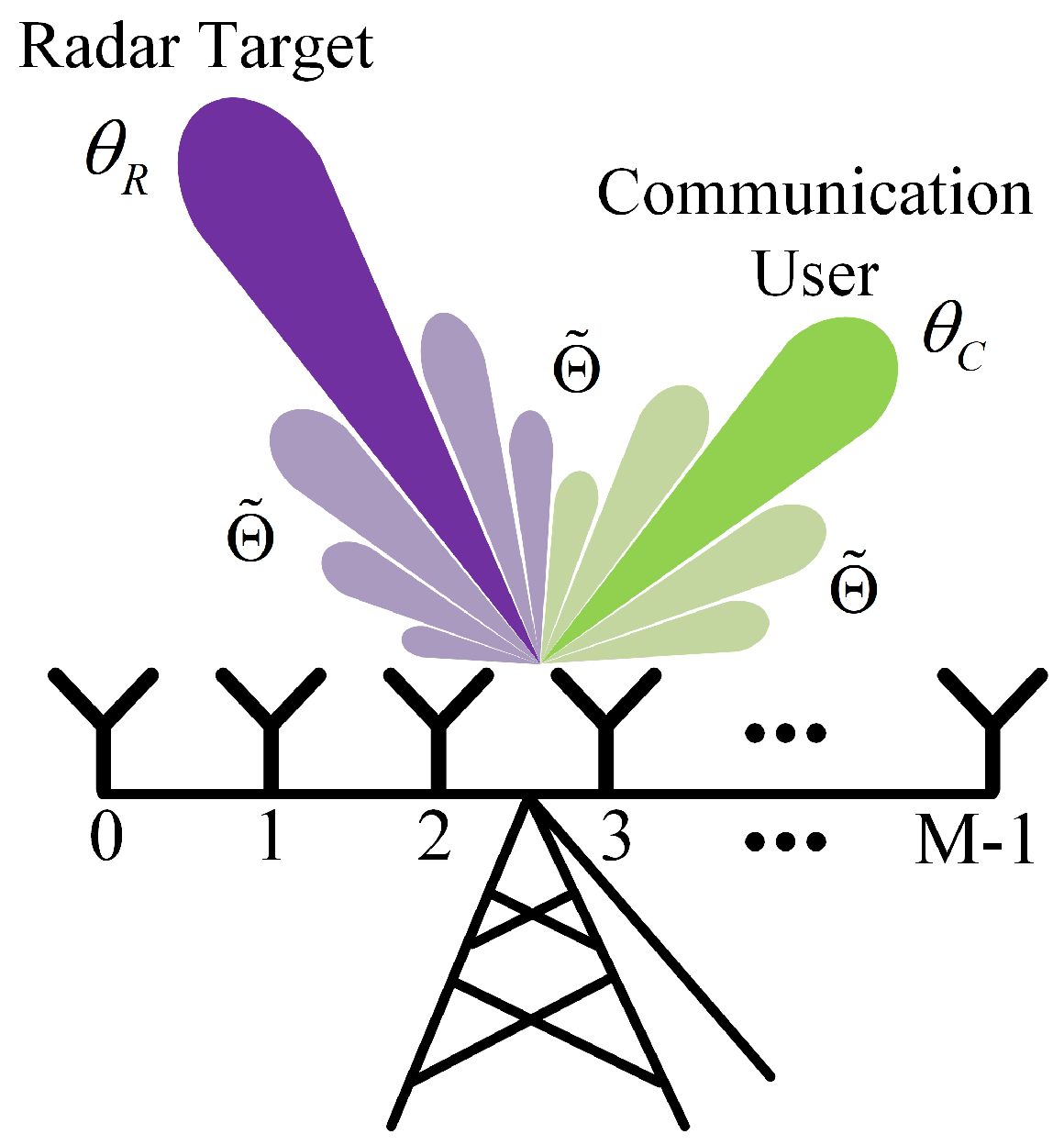
2. Signal Model and Problem Description

In this section, we present a DFRC transmit signal model based on uncertainty sets in the MIMO DFRC system. Then, the optimization problem for the robust low-sidelobe waveform design is formulated.

2.1. DFRC Transmit Signal Model

As illustrated in Figure 1, a MIMO DFRC system with a uniform linear array (ULA) consisting of M antennas is considered. Each element can transmit individual waveforms, enabling the simultaneous synthesis of radar and communication waveforms in the target and user directions. Therefore, the two functions can work simultaneously within the same spectrum, rather than requiring separate spectra. Let the discrete transmit waveform from the mth antenna be denoted as $x_m\left(n\right)$, where $m=0,\dots ,M-1$ and $n=0,\dots ,N-1$, with N representing the waveform length. Hence, all the transmit waveform can be formulated as the $M\times N$ waveform matrix $\mathbf{X}=\left[\mathbf{x}\left(0\right),\cdots ,\mathbf{x}\left(N-1\right)\right]$, where $\mathbf{x}\left(n\right)={\left[x_0\left(n\right),\cdots ,x_{M-1}\left(n\right)\right]}^T$, and $\mathbf{X}$ is to be optimized. We define the desired radar as ${\mathbf{s}}_R={\left[s_R\left(0\right),\cdots ,s_R\left(N-1\right)\right]}^T$ and the desired communication as ${\mathbf{s}}_C=\left[s_C\left(0\right),\right.$$\cdots ,{\left.s_C\left(N-1\right)\right]}^T$. Hence, to synthesize the desired waveforms simultaneously, $\mathbf{X}$ of the MIMO DFRC system needs to satisfy

$$\begin{array}{c}\hfill {\mathbf{a}}^H\left({\theta }_R\right)\mathbf{X}={\mathbf{s}}_R^T,\end{array}$$

(1)

$$\begin{array}{c}\hfill {\mathbf{a}}^H\left({\theta }_C\right)\mathbf{X}={\mathbf{s}}_C^T,\end{array}$$

(2)

where ${\theta }_R$ is the target direction, ${\theta }_C$ is the user direction, and we assume that ${\theta }_R\ne {\theta }_C$. In (1) and (2), the steering vector is defined as $\mathbf{a}\left(\theta \right)={[1,\cdots ,e^{-j{\displaystyle \frac{2\pi }{\lambda }}\left(M-1\right)dsin\theta }]}^H$, where d is the antenna interval, and $\lambda$ is the wavelength. To satisfy (1) and (2) in [39], $\mathbf{X}$ is represented as the combination of the radar transmit waveform ${\mathbf{X}}_R$ and the communication transmit waveform ${\mathbf{X}}_C$, where ${\mathbf{X}}_R={\mathbf{w}}_R{\mathbf{s}}_R^T$ and ${\mathbf{X}}_C={\mathbf{w}}_C{\mathbf{s}}_C^T$. Therefore, $\mathbf{X}$ can be represented as

$$\mathbf{X}={\mathbf{X}}_R+{\mathbf{X}}_C={\mathbf{w}}_R{\mathbf{s}}_R^T+{\mathbf{w}}_C{\mathbf{s}}_C^T.$$

(3)

In this case, the optimal $\mathbf{X}$ is derived by optimizing the radar and communication pre-coding weight vectors ${\mathbf{w}}_R$ and ${\mathbf{w}}_C$.

However, in practice, amplitude–phase errors in the MIMO DFRC system are inevitable. Even after calibration, residual array amplitude and phase errors still exist. These errors lead to a deviation between the ideal and real steering vectors, increase the sidelobe of transmit beampattern, and distort the synthesized waveforms in the target and user directions. Hence, the performance of the MIMO DFRC system degrades. To address this issue, we propose a robust low-sidelobe MIMO DFRC waveform design method when there are amplitude–phase errors.

2.2. Problem Formulation

Under amplitude–phase errors in a MIMO DFRC system, the real steering vector $\tilde{\mathbf{a}}\left(\theta \right)$ deviates from its ideal one. As stated in [45], it is represented as $\tilde{\mathbf{a}}\left(\theta \right)=\mathbf{a}\left(\theta \right)+\mathbf{e}\left(\theta \right)$, where $\mathbf{a}\left(\theta \right)$ is the ideal steering vector, and $\mathbf{e}\left(\theta \right)$ denotes the unknown error component. The error vector $\mathbf{e}\left(\theta \right)$ belongs to the uncertainty set

$$\mathsf{\Sigma }=\left\{\mathbf{e}\left(\theta \right)\left|{∥\mathbf{e}\left(\theta \right)∥}_2\le \epsilon \right.\right\},$$

(4)

where $\epsilon$ represents the upper bound of the modulus of the error vector, and $0<\epsilon <{∥\mathbf{a}\left(\theta \right)∥}_2=\sqrt{M}$.

Replacing the ideal steering vectors $\mathbf{a}\left({\theta }_R\right)$ in (1) and $\mathbf{a}\left({\theta }_C\right)$ in (2) with the real steering vectors $\tilde{\mathbf{a}}\left({\theta }_R\right)$ and $\tilde{\mathbf{a}}\left({\theta }_C\right)$, and substituting (3) into (1) and (2), we obtain

$$\begin{array}{c}\hfill {\tilde{\mathbf{a}}}^H\left({\theta }_R\right){\mathbf{w}}_R{\mathbf{s}}_R^T+{\tilde{\mathbf{a}}}^H\left({\theta }_R\right){\mathbf{w}}_C{\mathbf{s}}_C^T={\mathbf{s}}_R^T,\end{array}$$

(5)

$$\begin{array}{c}\hfill {\tilde{\mathbf{a}}}^H\left({\theta }_C\right){\mathbf{w}}_R{\mathbf{s}}_R^T+{\tilde{\mathbf{a}}}^H\left({\theta }_C\right){\mathbf{w}}_C{\mathbf{s}}_C^T={\mathbf{s}}_C^T,\end{array}$$

(6)

where ${\tilde{\mathbf{a}}}^H\left({\theta }_R\right){\mathbf{w}}_C{\mathbf{s}}_C^T$ can be regarded as the interference from the communication to the radar signals, and ${\tilde{\mathbf{a}}}^H\left({\theta }_C\right){\mathbf{w}}_R{\mathbf{s}}_R^T$ can be regarded as the interference from the radar to the communication signals. The distortion in the synthesized waveforms is mainly caused by the interference.

To minimize the sidelobe power of transmit beampattern and satisfy the constraints in (5) and (6), the robust low-sidelobe MIMO DFRC waveform design method can be formulated as

$$\begin{array}{cc}\hfill \underset{{\mathbf{w}}_R,{\mathbf{w}}_C}{min}& {∥{\mathbf{A}}^H(\tilde{\mathsf{\Theta }})\left({\mathbf{w}}_R{\mathbf{s}}_R^T+{\mathbf{w}}_C{\mathbf{s}}_C^T\right)∥}_F^2\hfill \end{array}$$

(7a)

$$\begin{array}{cc}\hfill \mathrm{s}.\mathrm{t}.& \left|{\mathbf{w}}_R^H\tilde{\mathbf{a}}\left({\theta }_R\right)\right|\ge 1\hfill \end{array}$$

(7b)

$$\begin{array}{cc}\hfill & \left|{\mathbf{w}}_R^H\tilde{\mathbf{a}}\left({\theta }_C\right)\right|\le \beta \hfill \end{array}$$

(7c)

$$\begin{array}{cc}\hfill & \left|{\mathbf{w}}_C^H\tilde{\mathbf{a}}\left({\theta }_C\right)\right|\ge 1\hfill \end{array}$$

(7d)

$$\begin{array}{cc}\hfill & \left|{\mathbf{w}}_C^H\tilde{\mathbf{a}}\left({\theta }_R\right)\right|\le \beta \hfill \end{array}$$

(7e)

$$\begin{array}{cc}\hfill & {∥{\mathbf{w}}_R∥}_2^2=1,{∥{\mathbf{w}}_C∥}_2^2=1\hfill \\ \hfill & \forall \mathbf{e}\left({\theta }_R\right),\mathbf{e}\left({\theta }_C\right)\in \mathsf{\Sigma },\hfill \end{array}$$

(7f)

where $\mathbf{A}(\tilde{\mathsf{\Theta }})=\left[\mathbf{a}\left({\theta }_1\right),\mathbf{a}\left({\theta }_2\right),\cdots ,\mathbf{a}\left({\theta }_Q\right)\right]$ is composed of the ideal steering vectors in the sidelobe directions, and $\tilde{\mathsf{\Theta }}=\left\{{\theta }_1,{\theta }_2,\cdots ,{\theta }_Q\right\}$ represents the set of angles in the sidelobe; $0<\beta \ll 1$. In this paper, the radar and communication mainlobes were treated as the mainlobes of the transmit beampattern, while the remaining components were regarded as the sidelobe angular range. In (7a), the objective function represents the transmit power in the sidelobe of the beampattern. Constraints in (7b) and (7d) ensure that the waveforms can be synthesized in their respective target and user directions. Additionally, constraints in (7c) and (7e) ensure that the mutual interference is suppressed. The constraint in (7f) is to control the total transmit power. Note that both $\left|{\mathbf{w}}_R^H\tilde{\mathbf{a}}\left({\theta }_R\right)\right|$ in (7b) and $\left|{\mathbf{w}}_C^H\tilde{\mathbf{a}}\left({\theta }_C\right)\right|$ in (7d) have upper bounds, since the moduli of the error steering vectors are limited.

Solving the optimization problem in (7), the optimal pre-coding weights are obtained, and substituting them into (3), the optimal $\mathbf{X}$ is achieved. In the following, we discuss how to solve the problem in (7).

3. Robust Low-Sidelobe MIMO DFRC Waveform Design

In this section, a robust low-sidelobe MIMO DFRC radar and communication waveform design method is proposed, and the computational complexity and convergence are analyzed.

3.1. Problem Relaxation

The optimization problem in (7) is challenging due to (1) the coupled variables in (7a) and (2) the non-convex and nonlinear constraints in (7b)–(7f). Therefore, the optimization problem in (7) needs to be relaxed. Based on the triangle inequality, the objective function in (7a) satisfies

$$\begin{array}{c}\hfill \begin{array}{cc}\hfill {∥{\mathbf{A}}^H(\tilde{\mathsf{\Theta }})\left({\mathbf{w}}_R{\mathbf{s}}_R^T+{\mathbf{w}}_C{\mathbf{s}}_C^T\right)∥}_F^2\le & {∥{\mathbf{A}}^H(\tilde{\mathsf{\Theta }}){\mathbf{w}}_R{\mathbf{s}}_R^T∥}_F^2+{∥{\mathbf{A}}^H(\tilde{\mathsf{\Theta }}){\mathbf{w}}_C{\mathbf{s}}_C^T∥}_F^2.\hfill \end{array}\end{array}$$

(8)

According to (8), the problem in (7) is relaxed as two optimization problems

$$\begin{array}{cc}\hfill \underset{{\mathbf{w}}_R}{min}& {∥{\mathbf{A}}^H(\tilde{\mathsf{\Theta }}){\mathbf{w}}_R{\mathbf{s}}_R^T∥}_F^2\hfill \end{array}$$

(9a)

$$\begin{array}{cc}\hfill \mathrm{s}.\mathrm{t}.& \left|{\mathbf{w}}_R^H\tilde{\mathbf{a}}\left({\theta }_R\right)\right|\ge 1\hfill \end{array}$$

(9b)

$$\begin{array}{cc}\hfill & \left|{\mathbf{w}}_R^H\tilde{\mathbf{a}}\left({\theta }_C\right)\right|\le \beta \hfill \end{array}$$

(9c)

$$\begin{array}{cc}\hfill & {∥{\mathbf{w}}_R∥}_2^2=1\hfill \\ \hfill & \forall \mathbf{e}\left({\theta }_R\right),\mathbf{e}\left({\theta }_C\right)\in \mathsf{\Sigma },\hfill \end{array}$$

(9d)

$$\begin{array}{cc}\hfill \underset{{\mathbf{w}}_C}{min}& {∥{\mathbf{A}}^H(\tilde{\mathsf{\Theta }}){\mathbf{w}}_C{\mathbf{s}}_C^T∥}_F^2\hfill \\ \hfill \mathrm{s}.\mathrm{t}.& \left|{\mathbf{w}}_C^H\tilde{\mathbf{a}}\left({\theta }_C\right)\right|\ge 1\hfill \\ \hfill & \left|{\mathbf{w}}_C^H\tilde{\mathbf{a}}\left({\theta }_R\right)\right|\le \beta \hfill \\ \hfill & {∥{\mathbf{w}}_C∥}_2^2=1\hfill \\ \hfill & \forall \mathbf{e}\left({\theta }_R\right),\mathbf{e}\left({\theta }_C\right)\in \mathsf{\Sigma }.\hfill \end{array}$$

(10)

Since the optimization problems in (9) and (10) are similar, our discussion focuses only on solving (9). The problem in (10) can be solved by same approach.

In (9), based on the triangle inequality and the Cauchy–Schwarz inequality, it can be observed that

$$\begin{array}{cc}\hfill \left|{\mathbf{w}}_R^H\tilde{\mathbf{a}}\left({\theta }_R\right)\right|& =\left|{\mathbf{w}}_R^H\left[\mathbf{a}\left({\theta }_R\right)+\mathbf{e}\left({\theta }_R\right)\right]\right|\hfill \\ \hfill & \ge \left|{\mathbf{w}}_R^H\mathbf{a}\left({\theta }_R\right)\right|-\left|{\mathbf{w}}_R^H\mathbf{e}\left({\theta }_R\right)\right|\hfill \\ \hfill & \ge \left|{\mathbf{w}}_R^H\mathbf{a}\left({\theta }_R\right)\right|-\epsilon {∥{\mathbf{w}}_R∥}_2.\hfill \end{array}$$

(11)

At this point, the constraint in (9b) can be relaxed as

$$\left|{\mathbf{w}}_R^H\mathbf{a}\left({\theta }_R\right)\right|-\epsilon {∥{\mathbf{w}}_R∥}_2\ge 1.$$

(12)

Using (12), the optimization problem in (9) can be relaxed as

$$\begin{array}{cc}\hfill \underset{{\mathbf{w}}_R}{min}& {∥{\mathbf{A}}^H(\tilde{\mathsf{\Theta }}){\mathbf{w}}_R{\mathbf{s}}_R^T∥}_F^2\hfill \end{array}$$

(13a)

$$\begin{array}{cc}\hfill \mathrm{s}.\mathrm{t}.& \left|{\mathbf{w}}_R^H\mathbf{a}\left({\theta }_R\right)\right|-\epsilon {∥{\mathbf{w}}_R∥}_2\ge 1\hfill \end{array}$$

(13b)

$$\begin{array}{cc}\hfill & \left|{\mathbf{w}}_R^H\tilde{\mathbf{a}}\left({\theta }_C\right)\right|\le \beta ,\forall \mathbf{e}\left({\theta }_C\right)\in \mathsf{\Sigma }\hfill \end{array}$$

(13c)

$$\begin{array}{cc}\hfill & {∥{\mathbf{w}}_R∥}_2^2=1.\hfill \end{array}$$

(13d)

It can be observed that the mutual interference suppression constraint in (13c) and the transmit power constraint in (13d) are still non-convex and nonlinear. The optimal transmit waveform is derived in Section 3.2 by solving (13).

3.2. Optimal Transmit Waveform Design

In this section, the problem in (13) is solved. Using a similar approach, the optimal communication pre-coding weight vector can be derived. Then, the optimal transmit waveform $\mathbf{X}$ is obtained by using (3) and the derived optimal pre-coding weight vectors.

3.2.1. Pre-Coding Weight Vectors Optimized Based on Low-Sidelobe Criterion

Note that if the constraints in (13c) and (13d) are removed, the optimization problem in (13) can become convex. Therefore, the pre-coding weight vector ${\mathbf{w}}_R$ was first optimized by solving (13) without these constraints. Then, the obtained pre-coding weight vector ${\mathbf{w}}_R$ were further designed to satisfy the mutual interference suppression constraint in (13c) and the transmit power constraint in (13d).

Ignoring the constraints in (13c) and (13d), (13) can be relaxed as

$$\begin{array}{cc}\hfill \underset{{\mathbf{w}}_R}{min}& {∥{\mathbf{A}}^H(\tilde{\mathsf{\Theta }}){\mathbf{w}}_R{\mathbf{s}}_R^T∥}_F^2\hfill \end{array}$$

(14a)

$$\begin{array}{cc}\hfill \mathrm{s}.\mathrm{t}.& \left|{\mathbf{w}}_R^H\mathbf{a}\left({\theta }_R\right)\right|-\epsilon {∥{\mathbf{w}}_R∥}_2\ge 1.\hfill \end{array}$$

(14b)

The problem in (14) remains non-convex due to the absolute value term $\left|{\mathbf{w}}_R^H\mathbf{a}\left({\theta }_R\right)\right|$ in (14b). Notably, if ${\mathbf{w}}_R$ is the solution to (14), then $e^{j\phi }{\mathbf{w}}_R$ is also the solution for any $\phi$. Therefore, multiplying ${\mathbf{w}}_R$ by a specific phase $e^{j{\phi }_0}$, we can make sure that $\left|{\mathbf{w}}_R^H\mathbf{a}\left({\theta }_R\right)\right|=\mathrm{Re}\left\{{\mathbf{w}}_R^H\mathbf{a}\left({\theta }_R\right)\right\}$ and $\mathrm{Im}\left\{{\mathbf{w}}_R^H\mathbf{a}\left({\theta }_R\right)\right\}=0$. Then, the optimization problem in (14) can be transformed into

$$\begin{array}{cc}\hfill \underset{{\mathbf{w}}_R}{min}& {∥{\mathbf{A}}^H(\tilde{\mathsf{\Theta }}){\mathbf{w}}_R{\mathbf{s}}_R^T∥}_F^2\hfill \\ \hfill \mathrm{s}.\mathrm{t}.& Re\left\{{\mathbf{w}}_R^H\mathbf{a}\left({\theta }_R\right)\right\}\ge 1+\epsilon {∥{\mathbf{w}}_R∥}_2.\hfill \end{array}$$

(15)

The problem in (15) is convex, and it can be solved by using the CVX toolbox in [46]. The optimal solution obtained via CVX is denoted as $\mathbf{w}{R_{c}vx}^{*}$. Similarly, we can obtain the communication pre-coding weight vector as ${\mathbf{w}}_{C\_cvx}^{*}$.

However, the CVX has high computational complexity. To improve the computational efficiency, we propose a DFRC waveform design method based on the ADMM algorithm.

Let ${\mathbf{t}}_2=\left[\begin{array}{c}Re\left\{\mathbf{a}\left({\theta }_R\right)\right\}\\ Im\left\{\mathbf{a}\left({\theta }_R\right)\right\}\end{array}\right]$, $\mathbf{u}={\left[Re{\left\{{\mathbf{w}}_R\right\}}^{T}Im{\left\{{\mathbf{w}}_R\right\}}^T\right]}^T$, ${\mathbf{t}}_1=\left[\begin{array}{c}Im\left\{\mathbf{a}\left({\theta }_R\right)\right\}\\ -Re\left\{\mathbf{a}\left({\theta }_R\right)\right\}\end{array}\right]$, $\mathbf{P}=\left[\begin{array}{cc}\mathrm{Re}\left\{{\mathbf{A}}^H(\tilde{\mathsf{\Theta }})\right\}& -\mathrm{Im}\left\{{\mathbf{A}}^H(\tilde{\mathsf{\Theta }})\right\}\\ \mathrm{Im}\left\{{\mathbf{A}}^H(\tilde{\mathsf{\Theta }})\right\}& \mathrm{Re}\left\{{\mathbf{A}}^H(\tilde{\mathsf{\Theta }})\right\}\end{array}\right]$, and let us introduce the auxiliary variable $\mathbf{v}$, the optimization problem in (15) can be rewritten as

$$\begin{array}{cc}\hfill \underset{\mathbf{u},\mathbf{v}}{min}& {∥{\mathbf{P}}^T{\mathbf{us}}_R^T∥}_F^2\hfill \\ \hfill \mathrm{s}.\mathrm{t}.& {\mathbf{t}}_2^T\mathbf{v}\ge 1+\epsilon {∥\mathbf{v}∥}_2\hfill \\ \hfill & \mathbf{u}=\mathbf{v}.\hfill \end{array}$$

(16)

Let ${\mathcal{D}}_{\mathbf{v}}\triangleq \left\{\mathbf{v}\left|{\mathbf{t}}_2^T\mathbf{v}\ge 1+\epsilon {∥\mathbf{v}∥}_2\right.\right\}$ and the convex set ${\mathcal{D}}_{\mathbf{v}}$ be closed and nonempty. The optimization problem in (16) can be simplified as

$$\begin{array}{cc}\hfill \underset{\mathbf{u},\mathbf{v}}{min}& {∥{\mathbf{P}}^T\mathbf{u}{\mathbf{s}}_R^T∥}_F^2\hfill \end{array}$$

(17a)

$$\begin{array}{cc}\hfill \mathrm{s}.\mathrm{t}.& \mathbf{u}=\mathbf{v},\mathbf{v}\in {\mathcal{D}}_{\mathbf{v}}.\hfill \end{array}$$

(17b)

The augmented Lagrangian function for the problem in (17) is expressed as

$$L_{\rho }\left(\mathbf{u},\mathbf{v},\mathbf{r}\right)={∥{\mathbf{P}}^T{\mathbf{us}}_R^T∥}_F^2+{\displaystyle \frac{\rho }{2}}{∥\mathbf{u}-\mathbf{v}+\mathbf{r}∥}_2^2-{\displaystyle \frac{\rho }{2}}{∥\mathbf{r}∥}_2^2,$$

(18)

where $\rho$ is a penalty factor, and $\mathbf{r}$ is a scaled dual variable.

Based on the ADMM algorithm framework [47], the variables $\mathbf{u}$, $\mathbf{v}$, and $\mathbf{r}$ are iteratively optimized. The initial optimization framework is given by

$$\begin{array}{cc}\hfill {\mathbf{u}}^{\left(\psi +1\right)}& =arg\underset{\mathbf{u}}{min}{L}_{\rho }\left(\mathbf{u},{\mathbf{v}}^{\left(\psi \right)},{\mathbf{r}}^{\left(\psi \right)}\right)\hfill \end{array}$$

(19a)

$$\begin{array}{cc}\hfill {\mathbf{v}}^{\left(\psi +1\right)}& =arg\underset{\mathbf{v}}{min}{L}_{\rho }\left({\mathbf{u}}^{\left(\psi +1\right)},\mathbf{v},{\mathbf{r}}^{\left(\psi \right)}\right)\hfill \end{array}$$

(19b)

$$\begin{array}{cc}\hfill {\mathbf{r}}^{\left(\psi +1\right)}& ={\mathbf{r}}^{\left(\psi \right)}+{\mathbf{u}}^{\left(\psi +1\right)}-{\mathbf{v}}^{\left(\psi +1\right)}.\hfill \end{array}$$

(19c)

For the $\left(\psi +1\right)\mathrm{th}$ iteration, with ${\mathbf{v}}^{\left(\psi \right)}$ and ${\mathbf{r}}^{\left(\psi \right)}$ fixed, ${\mathbf{u}}^{(\psi +1)}$ is updated by solving

$${\nabla }_{\mathbf{u}}{L}_{\rho }\left({\mathbf{u}}^{(\psi +1)},{\mathbf{v}}^{\left(\psi \right)},{\mathbf{r}}^{\left(\psi \right)}\right)=\mathbf{0}.$$

(20)

Substituting (18) into (20) and simplifying, we obtain

$$\left[{\mathbf{s}}_R{\mathbf{s}}_R^T\mathbf{P}{\mathbf{P}}^T+\rho {\mathbf{I}}_{2M}\right]{\mathbf{u}}^{\left(\psi +1\right)}=\left[\rho {\mathbf{v}}^{\left(\psi \right)}-\rho {\mathbf{r}}^{\left(\psi \right)}\right].$$

(21)

From (21), we obtain ${\mathbf{u}}^{\left(\psi +1\right)}$ as

$${\mathbf{u}}^{\left(\psi +1\right)}={\left[{\mathbf{s}}_R{\mathbf{s}}_R^T\mathbf{P}{\mathbf{P}}^T+\rho {\mathbf{I}}_{2M}\right]}^{-1}\left[\rho {\mathbf{v}}^{\left(\psi \right)}-\rho {\mathbf{r}}^{\left(\psi \right)}\right].$$

(22)

When ${\mathbf{u}}^{\left(\psi +1\right)}$ and ${\mathbf{r}}^{\left(\psi \right)}$ are fixed, ${\mathbf{v}}^{\left(\psi +1\right)}$ can be updated by solving

$$\begin{array}{cc}\hfill \underset{{\mathbf{v}}^{\left(\psi +1\right)}}{min}& {∥{\mathbf{v}}^{\left(\psi +1\right)}-{\mathbf{u}}^{\left(\psi +1\right)}-{\mathbf{r}}^{\left(\psi \right)}∥}_2^2\hfill \end{array}$$

(23a)

$$\begin{array}{cc}\hfill \mathrm{s}.\mathrm{t}.& {\mathbf{t}}_2^T{\mathbf{v}}^{\left(\psi +1\right)}\ge 1+\epsilon {∥{\mathbf{v}}^{\left(\psi +1\right)}∥}_2.\hfill \end{array}$$

(23b)

The optimization problem in (23) is convex. To reduce complexity, taking the square on both sides of (23b), (23) can be relaxed as

$$\begin{array}{cc}\hfill \underset{{\mathbf{v}}^{\left(\psi +1\right)}}{min}& {∥{\mathbf{v}}^{\left(\psi +1\right)}-{\mathbf{u}}^{\left(\psi +1\right)}-{\mathbf{r}}^{\left(\psi \right)}∥}_2^2\hfill \end{array}$$

(24a)

$$\begin{array}{cc}\hfill \mathrm{s}.\mathrm{t}.& {\left[{\mathbf{t}}_2^T{\mathbf{v}}^{\left(\psi +1\right)}-1\right]}^2\ge {\epsilon }^2{\left[{\mathbf{v}}^{\left(\psi +1\right)}\right]}^T{\mathbf{v}}^{\left(\psi +1\right)}.\hfill \end{array}$$

(24b)

Then, the Lagrangian function for (24a) and (24b) can be expressed as

$$\begin{array}{cc}\hfill L_y\left({\mathbf{u}}^{\left(\psi +1\right)},{\mathbf{v}}^{\left(\psi +1\right)},{\mathbf{r}}^{\left(\psi \right)}\right)=& {∥{\mathbf{v}}^{\left(\psi +1\right)}-{\mathbf{u}}^{\left(\psi +1\right)}-{\mathbf{r}}^{\left(\psi \right)}∥}_2^2\hfill \\ \hfill & +y{\epsilon }^2{\left[{\mathbf{v}}^{\left(\psi +1\right)}\right]}^T{\mathbf{v}}^{\left(\psi +1\right)}-y{\left[{\mathbf{t}}_2^T{\mathbf{v}}^{\left(\psi +1\right)}-1\right]}^2,\hfill \end{array}$$

(25)

where the multiplier $y>0$. Let ${\nabla }_{\mathbf{v}}{L}_y=\mathbf{0}$, ${\mathbf{v}}^{\left(\psi +1\right)}$ be expressed as

$$\begin{array}{cc}\hfill {\mathbf{v}}^{\left(\psi +1\right)}=& {\left[\left(1+y{\epsilon }^2\right){\mathbf{I}}_{2M}-y{\mathbf{t}}_2{\mathbf{t}}_2^T\right]}^{-1}\left[{\mathbf{u}}^{\left(\psi +1\right)}+{\mathbf{r}}^{\left(\psi \right)}-y{\mathbf{t}}_2\right].\hfill \end{array}$$

(26)

Based on the matrix inversion lemma, (26) can be rewritten as

$$\begin{array}{cc}\hfill {\mathbf{v}}^{\left(\psi +1\right)}=& {\displaystyle \frac{1}{1+y{\epsilon }^2}}\left[{\mathbf{I}}_{2M}+{\displaystyle \frac{y{\mathbf{t}}_2{\mathbf{t}}_2^T}{1+y\left({\epsilon }^2-{\mathbf{t}}_2^T{\mathbf{t}}_2\right)}}\right]\left[{\mathbf{u}}^{\left(\psi +1\right)}+{\mathbf{r}}^{\left(\psi \right)}-y{\mathbf{t}}_2\right].\hfill \end{array}$$

(27)

Substituting (27) into the constraint in (24b), the optimal $y^{*}$ can be obtained by solving

$$g\left(y\right)=g_4{y}^4+g_3{y}^3+g_2{y}^2+g_{1}y+g_0=0,$$

(28)

where $g_4={\epsilon }^6\left({∥{\mathbf{t}}_2∥}_2^2-{\epsilon }^2\right)$, $g_3=2{\epsilon }^4\left({∥{\mathbf{t}}_2∥}_2^2-2{\epsilon }^2\right)$, $g_1=2{\epsilon }^2[2{\mathbf{t}}_2^T\mathbf{z}-\left({∥{\mathbf{t}}_2∥}_2^2-{\epsilon }^2\right){∥\mathbf{z}∥}_2^2-2]$, $g_0={\epsilon }^2{∥\mathbf{z}∥}_2^2-{\left({\mathbf{t}}_2^T\mathbf{z}-1\right)}^2$, and $g_2={\epsilon }^2\left[{∥{\mathbf{t}}_2∥}_2^2+2{\epsilon }^2\left({\mathbf{t}}_2^T\mathbf{z}-3\right)-\left({∥{\mathbf{t}}_2∥}_2^2-{\epsilon }^2\right){\left({\mathbf{t}}_2^T\mathbf{z}\right)}^2+{\left({∥{\mathbf{t}}_2∥}_2^2-{\epsilon }^2\right)}^2{∥\mathbf{z}∥}_2^2\right]$, with $\mathbf{z}={\mathbf{u}}^{\left(k+1\right)}+{\mathbf{r}}^{\left(k\right)}$. We can prove that $g_4>0$, $g_3>0$, $g_1<0$, and $g_0<0$ (please see Appendix A for detail). According to Descartes’s rule of signs [48], since the coefficients $g_4$, $g_3$, $g_2$, $g_1$, and $g_0$ in (28) have only once sign change, the quartic equation in (28) has only one positive root $y^{*}$. According to [49], the positive root $y^{*}$ has the analytic form

$$\begin{array}{cc}\hfill y^{*}=& -{\displaystyle \frac{g_3}{4g_4}}+{\displaystyle \frac{1}{2}}\sqrt{{\displaystyle \frac{g_3^2}{4g_4^2}}-{\displaystyle \frac{2g_2}{3g_4}}+\gamma }+{\displaystyle \frac{1}{2}}\sqrt{{\displaystyle \frac{g_3^2}{2g_4^2}}-{\displaystyle \frac{4g_2}{3g_4}}-\gamma +{\displaystyle \frac{-\frac{g_3^3}{g_4^3}+\frac{4g_3{g}_2}{g_4^2}-\frac{8g_1}{g_4}}{4\sqrt{\frac{g_3^2}{4g_4^2}-\frac{2g_2}{3g_4}+\gamma }}}},\hfill \end{array}$$

(29)

where $\gamma ={\displaystyle \frac{\sqrt[3]{2}{\gamma }_1}{3g_4\sqrt[3]{{\gamma }_2+\sqrt{-4{\gamma }_1^3+{\gamma }_2^2}}}}+{\displaystyle \frac{\sqrt[3]{{\gamma }_2+\sqrt{-4{\gamma }_1^3+{\gamma }_2^2}}}{3\sqrt[3]{2}{g}_4}}$, ${\gamma }_1=g_2^2-3g_3{g}_1+12g_4{g}_0$ and ${\gamma }_2=2g_2^2-9g_3{g}_2{g}_1+27g_4{g}_1^2+27g_3^2{g}_0-72g_4{g}_2{g}_0$. The optimal ${\mathbf{v}}^{\left(\psi +1\right)}$ is obtained by substituting $y^{*}$ into (27), yielding

$$\begin{array}{cc}\hfill {\mathbf{v}}^{\left(\psi +1\right)}=& {\displaystyle \frac{1}{1+y^{*}{\epsilon }^2}}\left[{\mathbf{I}}_{2M}+{\displaystyle \frac{y^{*}{\mathbf{t}}_2{\mathbf{t}}_2^T}{1+y^{*}\left({\epsilon }^2-{\mathbf{t}}_2^T{\mathbf{t}}_2\right)}}\right]·\left[{\mathbf{u}}^{\left(\psi +1\right)}+{\mathbf{r}}^{\left(\psi \right)}-y^{*}{\mathbf{t}}_2\right].\hfill \end{array}$$

(30)

When ${\mathbf{u}}^{\left(\psi +1\right)}$ and ${\mathbf{v}}^{\left(\psi +1\right)}$ are fixed, the scaled dual variable ${\mathbf{r}}^{\left(\psi +1\right)}$ can be obtained by using (19c).

Let the residuals $h_{\mathbf{uv}}={∥{\mathbf{u}}^{\left(\psi +1\right)}-{\mathbf{v}}^{\left(\psi +1\right)}∥}_2^2$ and $h_{\mathbf{vv}}={∥{\mathbf{v}}^{\left(\psi +1\right)}-{\mathbf{v}}^{\left(\psi \right)}∥}_2^2$. If $h_{\mathbf{uv}}\le {\mu }_{\mathbf{uv}}$ and $h_{\mathbf{vv}}\le {\mu }_{\mathbf{vv}}$, or the number of iterations $\psi >{\psi }_{max}$, the iteration process ends, where ${\mu }_{\mathbf{uv}}$ and ${\mu }_{\mathbf{vv}}$ are the thresholds. To improve the iteration speed, following the derivations in [50,51], for the $\left(\psi +1\right)$th iteration, the update for $\rho$ is expressed as

$${\rho }^{\left(\psi +1\right)}=\left\{\begin{array}{cc}2{\rho }^{\left(\psi \right)},\hfill & \mathrm{if}0.1h_{\mathbf{uv}}>h_{\mathbf{vv}}\hfill \\ 0.5{\rho }^{\left(\psi \right)},\hfill & \mathrm{if}0.1h_{\mathbf{vv}}>h_{\mathbf{uv}}\hfill \\ {\rho }^{\left(\psi \right)},\hfill & \mathrm{otherwise}.\hfill \end{array}\right.$$

(31)

Then, we can obtain the radar pre-coding weight vector as ${\mathbf{w}}_{R\_admm}^{*}$. Similarly, we can obtain the communication pre-coding weight vector as ${\mathbf{w}}_{C\_admm}^{*}$.

3.2.2. Pre-Coding Weight Vectors Design Based on Mutual Interference Suppression Constraint and Transmit Power Constraint

Without the mutual interference suppression constraint in (13c), the synthesized waveforms in the target and user directions are distorted due to the mutual interference. To suppress that interference, the radar pre-coding weight vector was further designed to make sure that the radar interference in the communication mainlobe was minimized. Similarly, the communication pre-coding weight was also further designed to ensure that the communication interference in the radar mainlobe was minimized.

Let the radar and communication pre-coding weight vectors obtained in Section 3.2.1 be ${\mathbf{w}}_R^{*}$ and ${\mathbf{w}}_C^{*}$, respectively. To satisfy the constraint in (13c), based on the concept of orthogonal projection, the interference from radar to communication signals can be minimized by projecting ${\mathbf{w}}_R^{*}$ onto the orthogonal complement space of the communication mainlobe. Similarly, the interference from communication to radar signals can be minimized by projecting ${\mathbf{w}}_C^{*}$ onto the orthogonal complement space of the radar mainlobe. To this end, the orthogonal complement space of the communication mainlobe is represented as

$${\mathbf{P}}_C^{\perp }={\mathbf{I}}_M-\mathbf{A}\left({\mathsf{\Theta }}_C\right){\left[{\mathbf{A}}^H\left({\mathsf{\Theta }}_C\right)\mathbf{A}\left({\mathsf{\Theta }}_C\right)\right]}^{-1}{\mathbf{A}}^H\left({\mathsf{\Theta }}_C\right),$$

(32)

where $\mathbf{A}\left({\mathsf{\Theta }}_C\right)=\left[\mathbf{a}\left({\theta }_{C_1}\right),\mathbf{a}\left({\theta }_{C_2}\right),\cdots \mathbf{a}\left({\theta }_{C_L}\right)\right]$ is composed of the steering vectors in the communication mainlobe, and ${\mathsf{\Theta }}_C=\left\{{\theta }_{C_1},{\theta }_{C_2},\cdots ,{\theta }_{C_L}\right\}$ represents the set of angles in the communication mainlobe. The orthogonal complement space of the radar mainlobe is represented as

$${\mathbf{P}}_R^{\perp }={\mathbf{I}}_M-\mathbf{A}\left({\mathsf{\Theta }}_R\right){\left[{\mathbf{A}}^H\left({\mathsf{\Theta }}_R\right)\mathbf{A}\left({\mathsf{\Theta }}_R\right)\right]}^{-1}{\mathbf{A}}^H\left({\mathsf{\Theta }}_R\right),$$

(33)

where $\mathbf{A}\left({\mathsf{\Theta }}_R\right)=\left[\mathbf{a}\left({\theta }_{R_1}\right),\mathbf{a}\left({\theta }_{R_2}\right),\cdots \mathbf{a}\left({\theta }_{R_J}\right)\right]$ is composed of the steering vectors in the radar mainlobe, and ${\mathsf{\Theta }}_R=\left\{{\theta }_{R_1},{\theta }_{R_2},\cdots ,{\theta }_{R_J}\right\}$ represents the set of angles in the radar mainlobe.

After projection, the radar pre-coding vector is expressed as

$${\widehat{\mathbf{w}}}_R^{*}={\mathbf{P}}_C^{\perp }{\mathbf{w}}_R^{*},$$

(34)

and the communication pre-coding vector is expressed as

$${\widehat{\mathbf{w}}}_C^{*}={\mathbf{P}}_R^{\perp }{\mathbf{w}}_C^{*}.$$

(35)

Finally, to satisfy the transmit power constraint in (13d), ${\widehat{\mathbf{w}}}_R^{*}$ and ${\widehat{\mathbf{w}}}_C^{*}$ are normalized as

$${\widehat{\mathbf{w}}}_R^{*}={\widehat{\mathbf{w}}}_R^{*}/\phantom{{\widehat{\mathbf{w}}}_R^{*}\sum _{m=1}^M\left|{\widehat{w}}_{R,m}^{*}\right|}\sum _{m=1}^M\left|{\widehat{w}}_{R,m}^{*}\right|,$$

(36)

$${\widehat{\mathbf{w}}}_C^{*}={\widehat{\mathbf{w}}}_C^{*}/\phantom{{\widehat{\mathbf{w}}}_C^{*}\sum _{m=1}^M\left|{\widehat{w}}_{C,m}^{*}\right|}\sum _{m=1}^M\left|{\widehat{w}}_{C,m}^{*}\right|.$$

(37)

Substituting the designed ${\widehat{\mathbf{w}}}_R^{*}$ in (36) and ${\widehat{\mathbf{w}}}_C^{*}$ in (37) into (3), the optimal transmit waveform ${\mathbf{X}}^{*}$ can be expressed as

$${\mathbf{X}}^{*}={\widehat{\mathbf{w}}}_R^{*}{\mathbf{s}}_R^T+{\widehat{\mathbf{w}}}_C^{*}{\mathbf{s}}_C^T.$$

(38)

The robust low-sidelobe MIMO DFRC waveform design method is summarized in

Table 1. Robust Low-Sidelobe MIMO DFRC Waveform Design.

Input	${\theta }_R$, ${\theta }_C$, $\epsilon$, ${\mathbf{s}}_R$, ${\mathbf{s}}_C$, ${\mathbf{w}}_R^{\left(0\right)}$, ${\mathbf{w}}_C^{\left(0\right)}$, M, ${\mu }_{\mathrm{uv}}$, ${\mu }_{\mathrm{vv}}$, ${\psi }_{max}$.
Step 1	while $h_{\mathbf{uv}}>{\mu }_{\mathbf{uv}}$ or $h_{\mathbf{vv}}>{\mu }_{\mathbf{vv}}$ and $\psi \le {\psi }_{max}$ do
	(1) Separate the real and imaginary components of
	$\mathbf{a}\left({\theta }_R\right)$, $\mathbf{a}\left({\theta }_C\right)$, $\mathbf{A}(\tilde{\mathsf{\Theta }})$, ${\mathbf{w}}_R^{\left(0\right)}$, and ${\mathbf{w}}_C^{\left(0\right)}$;
	(2) ${\mathbf{u}}^{\left(\psi \right)}$ is updated by (21);
	(3) ${\mathbf{v}}^{\left(\psi \right)}$ is updated by (29);
	(4) ${\mathbf{r}}^{\left(\psi \right)}$ is updated by (30);
	(5) $\psi =\psi +1$.
Step 2	Calculate ${\mathbf{P}}_R^{\perp }$ by (32) and ${\mathbf{P}}_C^{\perp }$ by (33);
Step 3	Calculate ${\widehat{\mathbf{w}}}_R^{*}$ by (34) and ${\widehat{\mathbf{w}}}_C^{*}$ by (35);
Step 4	Normalize ${\widehat{\mathbf{w}}}_R^{*}$ by (36) and ${\widehat{\mathbf{w}}}_C^{*}$ by (37);
Step 5	Calculate ${\mathbf{X}}^{*}$ by (38).
output	Transmit waveform matrix ${\mathbf{X}}^{*}$.

and is referred to as RLSD–ADMM. Note that Step 1 in Table 1 can be performed by using the CVX toolbox, which is referred to as RLSD–CVX in this paper.

3.3. Analysis of Computational Complexity and Convergence

3.3.1. Analysis of Computational Complexity

The computational complexity of the RLSD–ADMM method in Table 1 was analyzed as follows. Step 1(2) has a complexity of $\mathcal{O}\left(Q{M}^2\right)$, Step 1(3) $\mathcal{O}\left(M^2\right)$, and Step 1(4) $\mathcal{O}\left(M\right)$. Therefore, the complexity of Step 1 is $\mathcal{O}\left((Q{M}^2+M^2+M)\beta \right)\approx \mathcal{O}\left(\left(Q{M}^2\right)\beta \right)$, where $\beta$ denotes the iteration count. Step 2 has a complexity of $\mathcal{O}(M{J}^2+M{L}^2)$, Step 3 $\mathcal{O}\left(M^2\right)$, Step 4 $\mathcal{O}\left(M\right)$, and Step 5 $\mathcal{O}\left(MN\right)$. Consequently, the total complexity of RLSD-ADMM is $\mathcal{O}(\left(Q{M}^2\right)\beta +M{J}^2+M{L}^2+M^2+M+MN)$.

For the RLSD–CVX method, Step 1 has a complexity of $\mathcal{O}\left(\left(NQ{M}^2\right){\beta }^{\prime }\right)$, where ${\beta }^{\prime }$ represents the iteration count. Steps 2–5 have the same complexities as in RLSD-ADMM. Therefore, the total complexity of RLSD-CVX is $\mathcal{O}(\left(NQ{M}^2\right){\beta }^{\prime }+M{J}^2+M{L}^2+M^2+M+MN)$.

As observed, if the iteration number is the same for both methods, the RLSD–ADMM method has lower computational complexity than the RLSD–CVX method.

3.3.2. Analysis of Convergence

The convergence of the RLSD–ADMM method was analyzed based on the results in [47,52]. The Lyapunov function in the $\psi \mathrm{th}$ iteration in Table 1 was defined as

$$V^{\left(\psi \right)}={\displaystyle \frac{1}{\rho }}{\parallel {\mathbf{f}}^{\left(\psi \right)}-{\mathbf{f}}^{*}\parallel }_2^2+\rho {\parallel {\mathbf{v}}^{\left(\psi \right)}-{\mathbf{v}}^{*}\parallel }_2^2,$$

(39)

where $\mathbf{f}=\rho \mathbf{r}$, ${\mathbf{f}}^{*}$ and ${\mathbf{v}}^{*}$ are the optimal vectors for the corresponding vectors. Let $p\left(\mathbf{u}\right)$ be the objective function in (17a), i.e.,

$$p\left(\mathbf{u}\right)={∥{\mathbf{P}}^T\mathbf{u}{\mathbf{s}}_R^T∥}_F^2.$$

(40)

To simplify, let $p^{\left(\psi \right)}=p\left({\mathbf{u}}^{\left(\psi \right)}\right)$. Then, we obtain (please see Appendix B for detail)

$$V^{\left(\psi +1\right)}\le V^{\left(\psi \right)}-\rho {∥{\mathbf{q}}^{\left(\psi +1\right)}∥}_2^2-\rho {∥{\mathbf{v}}^{\left(\psi +1\right)}-{\mathbf{v}}^{\left(\psi \right)}∥}_2^2,$$

(41)

$$\begin{array}{cc}\hfill p^{\left(\psi +1\right)}-p^{*}\le & -{\left[{\mathbf{f}}^{\left(\psi +1\right)}\right]}^T{\mathbf{q}}^{\left(\psi +1\right)}-\rho {\left[{\mathbf{v}}^{\left(\psi +1\right)}-{\mathbf{v}}^{\left(\psi \right)}\right]}^T\left[-{\mathbf{q}}^{\left(\psi +1\right)}+{\mathbf{v}}^{\left(\psi +1\right)}-{\mathbf{v}}^{*}\right],\hfill \end{array}$$

(42)

$$p^{*}-p^{\left(\psi +1\right)}\le {\left({\mathbf{f}}^{*}\right)}^T{\mathbf{q}}^{\left(\psi +1\right)},$$

(43)

where $p^{*}$ is the optimal value of $p^{\left(\psi \right)}$ and ${\mathbf{q}}^{\left(\psi +1\right)}={\mathbf{u}}^{\left(k+1\right)}-{\mathbf{v}}^{\left(\psi +1\right)}$. From (41), we obtain that $V^{\left(\psi \right)}$ monotonically decreases as $\psi$ increases. Therefore, from (39), we obtain that both ${\mathbf{f}}^{\left(\psi \right)}$ and ${\mathbf{v}}^{\left(\psi \right)}$ are bounded. Taking the cumulative summation on both sides of (41) with respective to the iteration index $\psi$ and simplify, we obtain

$$\rho \sum _{\psi =0}^{\infty }\left[{\parallel {\mathbf{q}}^{\left(\psi +1\right)}\parallel }_2^2+{\parallel {\mathbf{v}}^{\left(\psi +1\right)}-{\mathbf{v}}^{\left(\psi \right)}\parallel }_2^2\right]\le V^{\left(0\right)},$$

(44)

which implies that the series ${\displaystyle \sum _{\psi =0}^{\infty }}[{∥{\mathbf{q}}^{\left(\psi +1\right)}∥}_2^2+{∥{\mathbf{v}}^{\left(\psi +1\right)}-{\mathbf{v}}^{\left(\psi \right)}∥}_2^2]$ is limited. According to the necessary condition for the convergence of a series, we obtain

$$\underset{\psi \to \infty }{lim}\left[{∥{\mathbf{q}}^{\left(\psi +1\right)}∥}_2^2+{∥{\mathbf{v}}^{\left(\psi +1\right)}-{\mathbf{v}}^{\left(\psi \right)}∥}_2^2\right]=0.$$

(45)

Since both ${∥{\mathbf{q}}^{\left(\psi +1\right)}∥}_2^2$ and ${∥{\mathbf{v}}^{\left(\psi +1\right)}-{\mathbf{v}}^{\left(\psi \right)}∥}_2^2$ are non-negative, we obtain $\underset{\psi \to \infty }{lim}{\mathbf{q}}^{\left(\psi +1\right)}=0$ and $\underset{\psi \to \infty }{lim}\left[{\mathbf{v}}^{\left(\psi +1\right)}-{\mathbf{v}}^{\left(\psi \right)}\right]=0$. Therefore, for (42) and (43), when $\psi$ tends towards infinity, we obtain

$$\underset{\psi \to \infty }{lim}{p}^{\left(\psi +1\right)}-p^{*}\le 0,$$

(46)

$$\underset{\psi \to \infty }{lim}{p}^{*}-p^{\left(\psi +1\right)}\le 0.$$

(47)

From (46) and (47), we obtain $\underset{\psi \to \infty }{lim}{p}^{\left(\psi +1\right)}=p^{*}$. Note that the Steps 2–5 are all linear calculations and do not affect the convergence. Consequently, the proposed RLSD–ADMM method in Table 1 is convergent.

4. Simulation Results

4.1. Performance Metrics

In this section, the waveform error, peak-to-sidelobe ratio (PSLR), mutual interference level (MIL), average gain in pulse compression in radar mainlobe, and symbol error rate (SER) are given to assess the performance of the waveform design method.

4.1.1. Waveform Error

The relative error between the desired and synthesized waveforms is defined as

$${\eta }_{i,n}={\displaystyle \frac{\left|{\stackrel{⌢}{\mathbf{a}}}^H\left({\theta }_i\right)\mathbf{x}\left(n\right)-s_i^T\left(n\right)\right.}{\left|s_i^T\left(n\right)\right|}},i=RorC.$$

(48)

To assess the waveform error, the average relative error is given by

$${\mathsf{\Psi }}_i={\displaystyle \frac{1}{N}}\sum _{n=1}^N{\eta }_{i,n},i=RorC.$$

(49)

The standard deviation of the relative error is given by

$${\sigma }_i=\sqrt{\sum _{n=1}^N{\left({\eta }_{i,n}-{\mathsf{\Psi }}_i/\phantom{\mathsf{\Psi }iN}N\right)}^2},i=RorC.$$

(50)

We can see that the smaller the ${\eta }_{i,n}$, ${\mathsf{\Psi }}_i$, and ${\sigma }_i$, the better the designed waveform.

4.1.2. Peak-to-Sidelobe Ratio

The PSLR is given by

$${\mathrm{PSLR}}_{\mathrm{i}}=10{log}_{10}{\displaystyle \frac{\left|P_i\right|}{\left|P_m\right|}},i=RorC,$$

(51)

where $P_R$ and $P_C$ represent the peak of the radar and communication mainlobe in the transmit beampattern, respectively, and $P_m$ represents the highest sidelobe of the transmit beampattern. We can see that the larger the ${\mathrm{PSLR}}_{\mathrm{i}}$, the better the designed waveform.

4.1.3. Mutual Interference Level

To assess the mutual interference, the interference from radar to communication signals is defined as

$${\mathrm{MIL}}_{\mathrm{R}}={\displaystyle \frac{1}{L}}\sum _{l=1}^L{∥{\stackrel{⌢}{\mathbf{a}}}^H\left({\theta }_l\right){\mathbf{w}}_R{\mathbf{s}}_R^T}_2^2,$$

(52)

where $\stackrel{⌢}{\mathbf{a}}\left(\theta \right)$ represents the real steering vector. The interference from communication to radar signals is defined as

$${\mathrm{MIL}}_{\mathrm{C}}={\displaystyle \frac{1}{J}}\sum _{j=1}^J{∥{\stackrel{⌢}{\mathbf{a}}}^H\left({\theta }_j\right){\mathbf{w}}_C{\mathbf{s}}_C^T}_2^2.$$

(53)

We can see that the smaller the ${\mathrm{MIL}}_{\mathrm{R}}$ and ${\mathrm{MIL}}_{\mathrm{C}}$, the better the designed waveform.

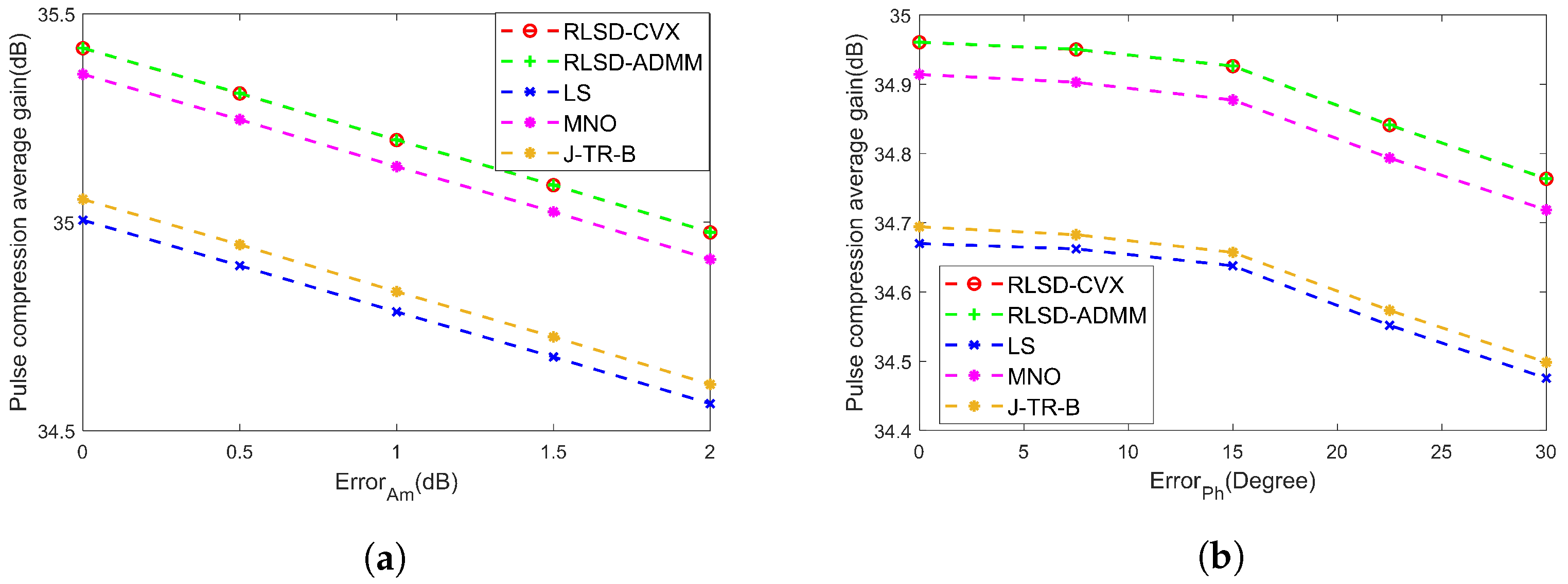
4.1.4. Average Gain of Pulse Compression in Radar Mainlobe

To assess the synthesized radar waveforms’ performance in the radar mainlobe, the average gain in pulse compression in the radar mainlobe is defined as

$$\mathsf{\Gamma }={\displaystyle \frac{1}{J}}\sum _{j=1}^J\left[{\stackrel{⌢}{\mathbf{a}}}^H\left({\theta }_j\right)\mathbf{X}\right]·{\mathbf{s}}_R.$$

(54)

We can see that the larger the $\mathsf{\Gamma }$, the better the designed waveform.

4.1.5. Symbol Error Rate

To assess the communication performance, the SER is defined as

$$\mathrm{SER}={\displaystyle \frac{N_e}{N_a}},$$

(55)

where $N_a$ is the communication symbol number and $N_e$ is the error symbol number. We can see that a smaller SER indicates better waveform performance.

4.2. Simulation

In the following simulations, a MIMO DFRC system with a ULA of 16 elements was considered, where the interval was half a wavelength. The desired radar waveform was a linear frequency modulation (LFM) signal targeting 0°, with a time-bandwidth product of 64. The desired communication waveform was a quadrature phase shift keying (QPSK) signal directed at 45°, with a bandwidth of 6.4 MHz. Since the radar waveform traveled in a round-trip link and the communication waveform traveled in a one-way link, the radar waveform transmit power was set 10 dB higher than the communication waveform transmit power. In the MIMO DFRC system, we assumed that the amplitude error among different elements obeyed the uniform distribution from $-2$ dB to 2 dB and the phase error among different elements obeyed the uniform distribution from −10° to 10°. The grid interval of angle was set to 0.1°. The results were averaged over 1000 Monte Carlo trials. The maximum iteration count was 2000, and the thresholds ${\mu }_{\mathbf{uv}}$ and ${\mu }_{\mathbf{vv}}$ were set to ${10}^{-5}$.

4.2.1. Convergence Analysis

For the proposed RLSD–ADMM method, Figure 2 shows the relations of radar residuals $h{r}_{\mathbf{uv}}$ and $h{r}_{\mathbf{vv}}$, as well as the communication residuals $h{c}_{\mathbf{uv}}$ and $h{c}_{\mathbf{vv}}$ with different iterations. As observed, these residuals decreased as the number of iterations increased. Hence, the proposed RLSD–ADMM method in Table 1 is convergent, which is consistent with the analysis in Section 3.3.2.

The computational times of the RLSD–CVX and RLSD–ADMM methods are presented in

Table 2. Computational Time.

Method	${\mathbf{w}}_{\mathit{R}}$	${\mathbf{w}}_{\mathit{C}}$
RLSD-CVX	59.18 s	59.88 s
RLSD-ADMM	0.32 s	0.32 s

, based on experiments conducted on a computer with a 2.5 GHz CPU and 16 GB of memory. The length of the transmit waveform was $N=256$. As shown, the RLSD-ADMM method was better than the RLSD–CVX method in terms of computational speed.

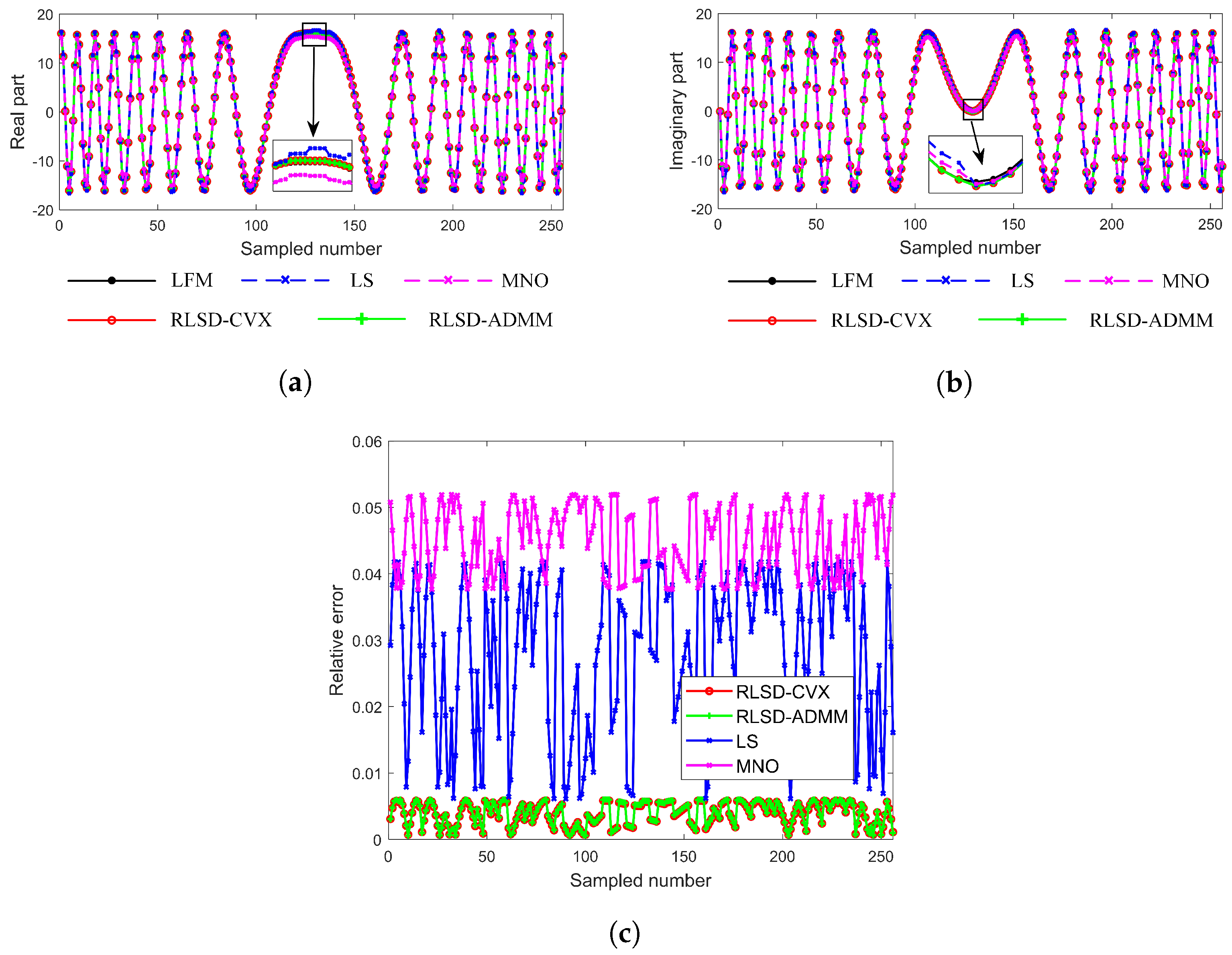
4.2.2. Waveform Error

The synthesized radar and communication waveforms are displayed in Figure 3 and Figure 4, respectively. For comparison, the radar and communication synthesized waveforms by the linear superposition (LS) method [39] and minimum norm optimization (MNO) method [40] are also illustrated. In Figure 3a,b, compared with the LS and MNO methods, the real and imaginary components of the radar waveform synthesized by the proposed robust methods demonstrated a closer match to the desired waveform. For the relative error between the desired and synthesized radar waveforms in Figure 3c, the proposed robust methods’ errors were less than 0.01, lower than those of the LS and MNO methods. Additionally,

Table 3. Waveform Error.

Method	${\mathsf{\Psi }}_{\mathit{R}}$	${\mathsf{\Psi }}_{\mathit{C}}$	${\mathit{\sigma }}_{\mathit{R}}$	${\mathit{\sigma }}_{\mathit{C}}$
LS	2.8 × ${10}^{-2}$	$1.3\times {10}^{-1}$	$3.4\times {10}^{-2}$	$2.7\times {10}^{-2}$
MNO	$4.5\times {10}^{-2}$	$3.8\times {10}^{-2}$	$6.6\times {10}^{-3}$	$5.6\times {10}^{-2}$
RLSD-CVX	$3.9\times {10}^{-3}$	$2.5\times {10}^{-2}$	$7.0\times {10}^{-4}$	$1.0\times {10}^{-2}$
RLSD-ADMM	$4.0\times {10}^{-3}$	$2.5\times {10}^{-2}$	$7.6\times {10}^{-4}$	$1.1\times {10}^{-2}$

provides a summary of the average relative error ${\mathsf{\Psi }}_R$ and the standard deviation of the relative error ${\sigma }_R$ for the various methods.

In Figure 4a,b, compared with the LS and MNO methods, the real and imaginary components of the communication waveform synthesized by the proposed robust methods demonstrated a closer match to the desired waveform. For the relative error between the desired and synthesized communication waveforms in Figure 4c, the proposed robust methods’ errors were less than 0.04, lower than those of the LS and MNO methods. Additionally, Table 3 also provides a summary of the average relative error ${\mathsf{\Psi }}_C$ and the standard deviation of the relative error ${\sigma }_C$ for the various methods.

In Table 3, compared with the LS and MNO methods, the proposed robust methods had much lower average relative error $\mathsf{\Psi }$ and standard deviation of the relative error $\sigma$. This implies that the RLSD–ADMM and RLSD–CVX methods are more robust to the amplitude and phase errors.

4.2.3. Transmit Beampattern

The radar and communication transmit beampatterns formed by ${\mathbf{X}}_R$ and ${\mathbf{X}}_C$ are depicted in Figure 5a and Figure 5b, respectively. The transmit beampattern formed by $\mathbf{X}$ is shown in Figure 5c. In Figure 5, the transmit beampatterns formed by the LS method [39] are also illustrated for comparison. As observed, the proposed robust methods resulted in a significantly lower sidelobe of the transmit beampattern compared to the LS method. In Figure 5a, the proposed methods created a null in the mainlobe direction of communication. Hence, the interference from radar to communication signals could be suppressed. Similarly, in Figure 5b, a null was formed in the mainlobe direction of radar. Hence, the interference from communication to radar signals could be suppressed. Moreover, Figure 5c shows that the transmit power in the communication direction was approximately 10 dB lower than that in the radar direction, which was consistent with the simulation parameters. The PSLR and MIL of different methods are summarized in

Table 4. Results of PSLR and MIL for different methods.

Method	PSLRR/dB	PSLRC/dB	MILR/dB	MILC/dB
LS	13.03	3.20	−1.17	−9.90
RLSD-CVX	17.01	7.09	−2.41	−12.64
RLSD-ADMM	17.01	7.10	−2.41	−12.65

.

Table 4 presents a comparison of PSLR and MIL values between the proposed robust methods and the LS method. The results indicate that the RLSD–ADMM and RLSD–CVX approaches achieve higher PSLR and lower MIL, demonstrating robustness against the amplitude–phase errors.

4.2.4. Pulse Compression Gain in Radar Mainlobe

In Figure 6, compared with the LS method [39], the MNO method [40], and the J–TR–B method [53], the proposed robust methods had a higher pulse compression gain in the radar mainlobe. For both RLSD–CVX and RLSW–ADMM methods, the average gains in pulse compression in the radar mainlobe were 34.94 dB, while it was 34.65 dB for the LS method, 34.84 dB for the MNO method, and 34.67 dB for the J–TR–B method.

In Figure 7a and Figure 7b, the variations in the average gain in pulse compression in the radar mainlobe with the different amplitude and phase errors are shown, respectively. In Figure 7a, the fixed phase error was set to ±10°. Intuitively, the average gain in pulse compression in the radar mainlobe decreased as the amplitude error increased. In Figure 7b, the fixed amplitude error was set to ±2 dB. Similarly, the average gain in pulse compression in the radar mainlobe decreased as the amplitude error increased. Moreover, under the amplitude–phase errors, the proposed robust methods had a higher average gain in pulse compression in the radar mainlobe compared with the LS, MNO, and J–TR–B methods, as shown in Figure 7.

4.2.5. Symbol Error Rate

Figure 8 presents the variation in the communication SER as a function of the signal-to-noise ratio (SNR). The results indicated that the proposed robust methods achieved a lower SER compared to the LS, MNO, and J–TR–B methods. Moreover, they had very similar performance to the desired waveform.

In Figure 9a and Figure 9b, the variations in SER with the different amplitude and phase errors are shown, respectively. In Figure 9a, the SNR was set to 8 dB, and the fixed phase error was set to ±10°. As expected, the SER increased as the amplitude error increased. In Figure 9b, the SNR was set to 8 dB, and the fixed amplitude error was set to ±2 dB. Similarly, the SER increased as the phase error increased. Moreover, under the amplitude–phase errors, the proposed robust methods had a lower SER compared with the LS, MNO, and J–TR–B methods as shown in Figure 9.

5. Conclusions

In this paper, robust low-sidelobe MIMO DFRC waveform design methods were proposed to mitigate performance degradation resulting from amplitude–phase errors in MIMO DFRC systems. The proposed methods, i.e., the RLSD–CVX and RLSD–ADMM methods, could simultaneously synthesize the desired waveforms in the target and user directions, respectively, and they could achieve a much lower sidelobe of the transmit beampattern. Moreover, the RLSD–ADMM method was convergent and had lower computational complexity compared with the RLSD–CVX method. Compared with the LS, MNO, and J–TR–B methods, the proposed methods had much better performance in terms of waveform error, transmit beampattern, pulse compression gain in the radar mainlobe, and SER. In summary, the proposed methods have enhanced robustness against the amplitude–phase errors in MIMO DFRC systems.

References

1. Xu, Z.; Tang, B.; Ai, W.; Xie, Z.; Zhu, J. Radar Transceiver Design for Extended Targets Based on Optimal Linear Detector. IEEE Trans. Aerosp. Electron. Syst. 2025, 1–12. [Google Scholar]
2. Xu, Z.; Tang, B.; Ai, W.; Zhu, J. Relative Entropy Based Jamming Signal Design Against Radar Target Detection. IEEE Trans. Signal Process. 2025, 73, 1200–1215. [Google Scholar]
3. Zheng, L.; Lops, M.; Eldar, Y.C.; Wang, X. Radar and communication coexistence: An overview: A review of recent methods. IEEE Signal Process. Mag. 2019, 36, 85–99. [Google Scholar]
4. Mahal, J.A.; Khawar, A.; Abdelhadi, A.; Clancy, T.C. Spectral coexistence of MIMO radar and MIMO cellular system. IEEE Trans. Aerosp. Electron. Syst. 2017, 53, 655–668. [Google Scholar]
5. Li, B.; Petropulu, A.P. Joint transmit designs for coexistence of MIMO wireless communications and sparse sensing radars in clutter. IEEE Trans. Aerosp. Electron. Syst. 2017, 53, 2846–2864. [Google Scholar]
6. Liu, F.; Garcia-Rodriguez, A.; Masouros, C.; Geraci, G. Interfering channel estimation in radar-cellular coexistence: How much information do we need? IEEE Trans. Wirel. Commun. 2019, 18, 4238–4253. [Google Scholar]
7. Li, B.; Petropulu, A.P.; Trappe, W. Optimum co-design for spectrum sharing between matrix completion based MIMO radars and a MIMO communication system. IEEE Trans. Signal Process. 2016, 64, 4562–4575. [Google Scholar]
8. Xiao, B.; Huo, K.; Liu, Y.X. Development and prospect of radar and communication integration. J. Electron. Inf. Technol. 2019, 41, 739–750. [Google Scholar]
9. Zhang, J.A.; Liu, F.; Masouros, C.; Heath, R.W.; Feng, Z.; Zheng, L.; Petropulu, A. An overview of signal processing techniques for joint communication and radar sensing. IEEE J. Sel. Top. Signal Process. 2021, 15, 1295–1315. [Google Scholar]
10. Ma, S.; Sheng, H.; Yang, R.; Li, H.; Wu, Y.; Shen, C.; Al-Dhahir, N.; Li, S. Covert beamforming design for integrated radar sensing and communication systems. IEEE Trans. Wirel. Commun. 2023, 22, 718–731. [Google Scholar]
11. Zhao, N.; Wang, Y.; Zhang, Z.; Chang, Q.; Shen, Y. Joint transmit and receive beamforming design for integrated sensing and communication. IEEE Commun. Lett. 2022, 26, 662–666. [Google Scholar]
12. Kumari, P.; Choi, J.; Gonzlez-Prelcic, N.; Heath, R.W. IEEE 802.11ad based radar: An approach to joint vehicular communication-radar system. IEEE Trans. Veh. Technol. 2018, 67, 3012–3027. [Google Scholar]
13. Zhang, H.; Liu, W.; Zhang, Q.; Zhang, L.; Liu, B. Joint customer assignment, power allocation, and subchannel allocation in a UAV-based joint radar and communication network. IEEE Internet Things J. 2024, 11, 29643–29660. [Google Scholar]
14. Zhang, H.; Liu, W.; Zhang, Q.; Zhang, L.; Liu, B.; Xu, H.X. Joint power, bandwidth, and subchannel allocation in a UAV-assisted DFRC network. IEEE Internet Things J. 2025, 1–17. [Google Scholar]
15. Liu, Y.; Liao, G.; Yang, Z.; Xu, J. Multiobjective optimal waveform design for OFDM integrated radar and communication systems. Signal Process. 2017, 141, 331–342. [Google Scholar]
16. Yin, T.; Guo, W.; Zhu, J.; Wu, Y.; Zhang, B.; Zhou, Z. Underwater Broadband Target Detection by Filtering Scanning Azimuths Based on Features of Sub-band Peaks. IEEE Sens. J. 2025, 1–9. [Google Scholar]
17. Zhu, J.; Yin, T.; Guo, W.; Zhang, B.; Zhou, Z.; Liu, W. An Underwater Target Azimuth Trajectory Enhancement Approach in BTR. Appl. Acoust. 2025, 230, 110373. [Google Scholar]
18. Liu, Y.; Liao, G.; Xu, J.; Yang, Z.; Huang, L.; Zhang, Y. Transmit power adaptation for orthogonal frequency division multiplexing integrated radar and communication systems. J. Appl. Remote Sens. 2017, 11, 1–17. [Google Scholar]
19. Liu, Y.; Liao, G.; Xu, J.; Yang, Z.; Zhang, Y. Adaptive OFDM integrated radar and communications waveform design based on information theory. IEEE Commun. Lett. 2017, 21, 2174–2177. [Google Scholar]
20. Liu, Y.; Liao, G.; Yang, Z. Robust OFDM integrated radar and communications waveform design based on information theory. Signal Process. 2019, 162, 317–329. [Google Scholar]
21. Yuan, W.; Wei, Z.; Li, S.; Yuan, J.; Ng, D.W.K. Integrated sensing and communication-assisted orthogonal time frequency space transmission for vehicular networks. IEEE J. Sel. Top. Signal Process. 2021, 15, 1515–1528. [Google Scholar] [CrossRef]
22. Gaudio, L.; Kobayashi, M.; Caire, G.; Colavolpe, G. On the effectiveness of OTFS for joint radar parameter estimation and communication. IEEE Trans. Wirel. Commun. 2020, 19, 5951–5965. [Google Scholar] [CrossRef]
23. Zhu, J.; Xie, Z.; Jiang, N.; Song, Y.; Han, S.; Liu, W.; Huang, X. Delay-Doppler Map Shaping through Oversampled Complementary Sets for High Speed Target Detection. Remote Sens. 2024, 16, 2898. [Google Scholar] [CrossRef]
24. Karpovich, P.; Zielinski, T.P. Random-padded OTFS modulation for joint communication and radar/sensing systems. In Proceedings of the 2022 23rd International Radar Symposium (IRS), Gdansk, Poland, 12–14 September 2022; pp. 104–109. [Google Scholar]
25. Zhang, Y.; Li, Q.; Huang, L.; Pan, C.; Song, J. A Modified Waveform Design for Radar-Communication Integration Based on LFM-CPM. In Proceedings of the 2017 IEEE 85th Vehicular Technology Conference (VTC Spring), Sydney, NSW, Australia, 4–7 June 2017; pp. 1–5. [Google Scholar]
26. Chen, X.; Wang, X.; Xu, S.; Zhang, J. A novel radar waveform compatible with communication. In Proceedings of the 2011 International Conference on Computational Problem-Solving (ICCP), Chengdu, China, 21–23 October 2011; pp. 177–181. [Google Scholar]
27. Huang, T.; Shlezinger, N.; Xu, X.; Liu, Y.; Eldar, Y.C. MAJoRCom: Dual-function radar communication system using index modulation. IEEE Trans. Signal Process. 2020, 68, 3423–3438. [Google Scholar] [CrossRef]
28. Huang, T.; Shlezinger, N.; Xu, X.; Ma, D.; Liu, Y.; Eldar, Y.C. Multicarrier agile phased array radar. IEEE Trans. Signal Process. 2020, 68, 5706–5721. [Google Scholar] [CrossRef]
29. Sahin, A.; Hoque, S.S.M.; Chen, C.-Y. Index modulation with circularly-shifted chirps for dual-function radar and communications. IEEE Trans. Wirel. Commun. 2022, 21, 2938–2952. [Google Scholar] [CrossRef]
30. Hassanien, A.; Amin, M.G.; Zhang, Y.D.; Ahmad, F. A dual function radar-communications system using sidelobe control and waveform diversity. In Proceedings of the 2015 IEEE Radar Conference (RadarCon), Arlington, VA, USA, 10–15 May 2015; pp. 1260–1263. [Google Scholar]
31. Hassanien, A.; Amin, M.G.; Zhang, Y.D.; Ahmad, F. Dual-function radar-communications: Information embedding using sidelobe control and waveform diversity. IEEE Trans. Signal Process. 2016, 64, 2168–2181. [Google Scholar] [CrossRef]
32. Arik, M.; Akan, O.B. Utilizing sidelobe ASK based joint radar-communication system under fading. In Proceedings of the 2017 IEEE Military Communications Conference (MILCOM), Baltimore, MD, USA, 10–15 May 2017; pp. 623–628. [Google Scholar]
33. Hassanien, A.; Amin, M.G.; Zhang, Y.D. Phase-modulation based dual-function radar-communications. IET Radar Sonar Navig. 2016, 10, 1411–1421. [Google Scholar] [CrossRef]
34. Hassanien, A.; Zhang, Y.D.; Gu, Y. Dual-function radar-communications using QAM-based sidelobe modulation. Digit. Signal Process. 2018, 82, 166–174. [Google Scholar]
35. Liu, F.; Zhou, L.; Masouros, C.; Li, A.; Luo, W.; Petropulu, A. Toward dual-functional radar-communication systems: Optimal waveform design. IEEE Trans. Signal Process. 2018, 66, 4264–4279. [Google Scholar] [CrossRef]
36. Liu, F.; Masouros, C.; Li, A.; Sun, H.; Hanzo, L. MU-MIMO communications with MIMO radar: From coexistence to joint transmission. IEEE Trans. Wirel. Commun. 2018, 17, 2755–2770. [Google Scholar]
37. Liu, X.; Huang, T.; Shlezinger, N.; Liu, Y.; Zhou, J.; Eldar, Y.C. Joint Transmit Beamforming for Multiuser MIMO Communications and MIMO Radar. IEEE Trans. Signal Process. 2020, 68, 3929–3944. [Google Scholar]
38. Shi, S.; Wang, Z.; He, Z.; Cheng, Z. Constrained waveform design for dual-functional MIMO radar-communication system. Signal Process. 2020, 171, 107530. [Google Scholar] [CrossRef]
39. Jiang, M.; Liao, G.; Yang, Z.; Liu, Y.; Chen, Y.; Li, H. Integrated waveform design for an Integrated Radar and Communication System with a Uniform Linear Array. In Proceedings of the 2020 IEEE 11th Sensor Array and Multichannel Signal Processing Workshop (SAM), Hangzhou, China, 8–11 June 2020; pp. 1–5. [Google Scholar]
40. Jiang, M.; Liao, G.; Yang, Z.; Liu, Y.; Chen, Y. Integrated radar and communication waveform design based on a shared array. Signal Process. 2021, 182, 107956. [Google Scholar]
41. Wu, W.; Han, G.; Cao, Y.; Huang, Y.; Yeo, T.-S. MIMO waveform design for dual functions of radar and communication with space-time coding. IEEE J. Sel. Areas Commun. 2022, 40, 1906–1917. [Google Scholar]
42. Liu, X.; Liao, G.; Liu, Y.; Tang, H.; Wang, H. Low Sidelobe Integrated Radar and Communication Shared Waveform Design. In Proceedings of the 2023 3rd International Conference on Frontiers of Electronics, Information and Computation Technologies (ICFEICT), Yangzhou, China, 26–29 May 2023; pp. 559–563. [Google Scholar]
43. Feng, Y.; Liao, G.; Xu, J.; Zhu, S.; Zeng, C. Robust adaptive beamforming against large steering vector mismatch using multiple uncertainty sets. Signal Process. 2018, 152, 320–330. [Google Scholar] [CrossRef]
44. Huang, Y.; Vorobyov, S.A.; Luo, Z.-Q. Quadratic matrix inequality approach to robust adaptive beamforming for general-rank signal model. IEEE Trans. Signal Process. 2020, 68, 2244–2255. [Google Scholar]
45. Vorobyov, S.A.; Gershman, A.B.; Luo, Z.Q. Robust adaptive beamforming using worst-case performance optimization: A solution to the signal mismatch problem. IEEE Trans. Signal Process. 2003, 51, 1702–1715. [Google Scholar]
46. Grant, M.; Boyd, S. CVX: Matlab Software for Disciplined Convex Programming, version 2.1. March 2014. Available online: http://cvxr.com/cvx (accessed on 1 January 2020).
47. Boyd, S.; Parikh, N.; Chu, E.; Peleato, B.; Eckstein, J. Distributed optimization and statistical learning via the alternating direction method of multipliers. Found. Trends Mach. Learn. 2011, 3, 1–122. [Google Scholar]
48. Descartes, R.; Smith, D.E.; Latham, M.L. The Geometry of René Descartes: With a Facsimile of the First Edition, 1637; Dover Publications: Mineola, NY, USA, 1954. [Google Scholar]
49. Abramowitz, M. The Solutions of Quartic Equations. In Handbook of Mathematical Functions with Formulas, Graphs, Mathematical Tables; Dover Publications: Mineola, NY, USA, 1972; pp. 17–18. [Google Scholar]
50. He, B.S.; Yang, H.; Wang, S.L. Alternating Direction Method with Self-Adaptive Penalty Parameters for Monotone Variational Inequalities. J. Optim. Theory Appl. 2000, 106, 337–356. [Google Scholar]
51. Wang, S.; Liao, L. Decomposition Method with a Variable Parameter for a Class of Monotone Variational Inequality Problems. J. Optim. Theory Appl. 2001, 109, 415–429. [Google Scholar]
52. Liang, J.; So, H.C.; Li, J.; Farina, A. Unimodular Sequence Design Based on Alternating Direction Method of Multipliers. IEEE Trans. Signal Process. 2016, 64, 5367–5381. [Google Scholar]
53. Liu, Z.; Aditya, S.; Li, H.; Clerckx, B. Joint Transmit and Receive Beamforming Design in Full-Duplex Integrated Sensing and Communications. IEEE J. Sel. Areas Commun. 2023, 41, 2907–2919. [Google Scholar]
Figure 1. MIMO DFRC system transmit model diagram.
Remotesensing 17 01242 g001
Figure 2. Convergence curve.
Remotesensing 17 01242 g002
Figure 3. Performance of radar waveforms. (a) Real part of radar waveforms. (b) Imaginary part of radar waveforms. (c) Relative error between desired radar waveform and synthesized radar waveforms.
Remotesensing 17 01242 g003
Figure 4. Performance of communication waveforms. (a) Real part of communication waveforms. (b) Imaginary part of communication waveforms. (c) Relative error between desired communication waveform and synthesized communication waveforms.
Remotesensing 17 01242 g004
Figure 5. Transmit beampattern results. (a) Radar transmit beampattern. (b) Communication transmit beampattern. (c) Transmit beampattern.
Remotesensing 17 01242 g005
Figure 6. Pulse compression gain in radar mainlobe.
Remotesensing 17 01242 g006
Figure 7. Variations in average gain in pulse compression. (a) Average gain in pulse compression in the radar mainlobe versus amplitude error. (b) Average gain in pulse compression in the radar mainlobe versus phase error.
Remotesensing 17 01242 g007
Figure 8. SER versus SNR.
Remotesensing 17 01242 g008
Figure 9. The variations in SER. (a) SER versus amplitude error. (b) SER versus phase error.
Remotesensing 17 01242 g009