Automated Plasma Region Classification and Boundary Layer Identification Using Machine Learning

Abstract

The accurate classification of plasma regions is a critical challenge in space science, with identifying dynamic boundary layers (BLs) being particularly complex. This study introduces a novel wavelet-decision tree classifier (WDTC) designed to automate BL detection. Unlike conventional machine learning methods that rely on raw satellite measurements, the WDTC utilizes processed parameters derived from wavelet analysis as inputs to the decision tree algorithm. For each in situ measurement, including magnetic field strength (B), plasma density (n), velocity (V), and temperature (T), the wavelet analysis generates two features: wavelet energy and wavelet entropy. This results in a total of eight input parameters (two for each of the four in situ measurements) for the decision tree. By incorporating these distinctive wavelet-derived features, the WDTC enhances its ability to accurately and efficiently identify BLs within complex plasma environments. The model was applied to data from the Magnetospheric Multiscale (MMS) mission, focusing on the dayside region, and successfully differentiated between the solar wind, bow shock, magnetosheath, magnetopause, and magnetosphere. From September 15 to December 31, 2015, the WDTC identified 711 BL crossings, including 295 bow shock events and 416 magnetopause crossings. Beyond its scientific applications, the WDTC provides high-quality training datasets and a reliable data labeling tool, contributing to neural network training efforts.

1. Introduction

The supersonic solar wind frozen in the interplanetary magnetic field interacts with the Earth’s magnetosphere, creating a complex near-Earth space environment [1,2]. While the Earth’s magnetosphere derives all its energy from the solar wind, the magnetopause—where magnetic reconnection predominantly occurs—plays a critical role in regulating the transfer of solar wind energy into the magnetosphere and ionosphere [3,4]. Within this system, boundary layers such as the bow shock (BS) and magnetopause (MP) serve as demarcations between distinct plasma regions, including the solar wind (SW), magnetosheath (MSH), and magnetosphere (MSP) [5,6,7]. The time-varying solar wind activates these regions and boundary layers, resulting in dynamic behaviors that are critical for understanding the interaction between the solar wind and Earth’s magnetosphere [8,9,10]. Accurately identifying these plasma regions and delineating their boundaries is essential for advancing our understanding of space weather phenomena.

Recent advances in data-driven machine learning (ML) techniques have demonstrated significant potential for space weather applications, particularly in classification and forecasting tasks [11]. By utilizing MMS mission data, both supervised and unsupervised ML approaches have been successfully applied to automate plasma region classification and magnetopause identification [12], offering a more efficient and reliable alternative to conventional experience-based analytical approaches [13,14]. For example, probabilistic models, for instance, have been employed to identify the magnetopause [15]. In addition, more sophisticated methods such as convolutional neural networks (CNNs) have been used to classify 3D particle energy distributions [16]. Also, as described in [17], a long short-term memory (LSTM) neural network has been developed to predict magnetopause crossings in low-resolution time-series data, optimizing the MMS mission’s burst data selection process through automated analysis. Furthermore, in [18], the authors utilized fully convolutional networks (FCNs) to classify plasma regions within MMS datasets, surpassing traditional multi-layer perceptron (MLP) models and achieving superior accuracy when applied to cluster mission data.

Nevertheless, machine learning faces significant challenges when it comes to identifying boundary layers. The conventional approach to addressing these challenges often involves a two-step methodology. For instance, in [19], the authors employed a Gradient Boosting Classifier, a variant of decision trees, to develop an automated method for identifying three key near-Earth regions: the magnetosphere, magnetosheath, and solar wind. Once the spacecraft data are classified into these regions, the identification of specific boundaries becomes possible. In their study, magnetopause crossings were defined as epochs during which the number of magnetosheath and magnetosphere data points were balanced within a 1 h window. In contrast, bow shock crossings were characterized as periods where the counts of magnetosheath and solar wind data points were equal within a 10 min window.

In a similar approach, in [20], the authors employed a two-step strategy for identifying boundary layers, incorporating an unsupervised learning algorithm, the Gaussian Mixture Model (GMM), for clustering tasks. This methodology was further refined with feature generation and basic post-processing techniques, utilizing ion spectral data and total magnetic field measurements, as informed by the plasma region classification framework of [21]. The integrated approach was applied to automate the classification of MMS mission dayside observations into four primary plasma regions: the magnetosphere, magnetosheath, solar wind, and ion foreshock. Following this classification, the detection of magnetopause and bow shock crossings was achieved by analyzing the transitions between these regions. as described in [22], where the authors detected bow shock crossing times by computing probability differences, establishing thresholds, and applying a moving median filter for result smoothing.

In this research, we propose a novel wavelet decision tree classifier (WDTC) that combines plasma region classification and dynamic boundary layer identification into a unified framework. The WDTC utilizes wavelet transforms to extract time-varying features from raw physical measurements of field and plasma parameters, which are subsequently used to train a decision tree model. When applied to dayside plasma region data from the MMS mission, the WDTC effectively identifies five key plasma regions: the solar wind, bow shock, magnetosheath, magnetopause, and magnetosphere. The structure of the paper is as follows:

Section 1: Introduction. This section provides an overview of both conventional and machine learning methodologies employed for plasma region classification and boundary layer identification.

Section 2: Physical insight: The tripartite distribution from the solar wind to the magnetosphere. Here, we explore the physical implications of the three-segment distribution of plasma regions, from the solar wind to the magnetosphere.

Section 3: Data interpretation and labeled dataset. This section outlines the MMS mission’s instrumentation and the datasets used in this study, establishing the context for the subsequent analysis, and we introduce the labeled dataset, detailing the data preprocessing steps and label generation procedures.

Section 4: The WDTC model. We describe the WDTC model in this section, explaining the rationale behind the selection of the wavelet transform and decision tree algorithm, as well as performance evaluation methods.

Section 5: Model training. This section outlines the methods used for training the model, detailing the processes for feature evaluation and highlighting the steps taken to ensure the model’s effectiveness and robustness.

Section 6: Category results. Two case studies are presented in this section to demonstrate the categorization capabilities of the WDTC model. The first case study focuses on the identification of the magnetopause boundary, distinguishing the magnetosheath from the magnetosphere. The second case study examines the identification of the bow shock boundary, separating the solar wind from the magnetosheath.

Section 7: Discussion. In this section, we perform a comparative evaluation of wavelet transforms and Fast Fourier Transform (FFT) techniques, analyzing their respective advantages and limitations. Additionally, we assess the performance of the WDTC model against the GMM model proposed by [20] and critically evaluate the strengths and weaknesses of the WDTC approach in boundary layer identification.

Section 8: Conclusions. This section summarizes the key findings and conclusions of the study, providing a concise overview of the research outcomes.

2. Physical Insight: The Tripartite Distribution from the Solar Wind to the Magnetosphere

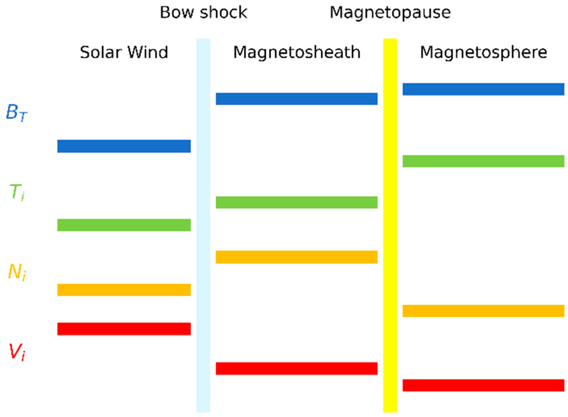
Figure 1 presents a schematic illustration of the segmentation of plasma parameters across distinct regions of near-Earth space. These parameters include the magnetic field (B), ion velocity (V), ion density (n), and ion temperature (T). The regions shown are the supersonic solar wind, the subsonic magnetosheath, and the magnetosphere. These regions are separated by the dynamic boundary layers of the bow shock and magnetopause. In the schematic diagram, both the magnetic field B and temperature T show a progressive increase from the solar wind to the magnetosphere, while ion velocity V gradually decreases. Ion density reaches its maximum in the magnetosheath and its minimum in the magnetosphere.

To directly examine the evolution of the magnetic field and plasma parameters across different plasma regions on the dayside, we performed a statistical analysis using data from the MMS mission. The magnetosheath and magnetosphere data were extracted from a one-month dataset collected by MMS in February 2016, while solar wind data were obtained from omni-directional observations during the same period. All data used in this study consist of 1 min averaged values. The dataset includes 28,476 data points for the solar wind, 8547 for the magnetosheath, and 1917 for the magnetosphere, each representing 1 min averaged measurements.

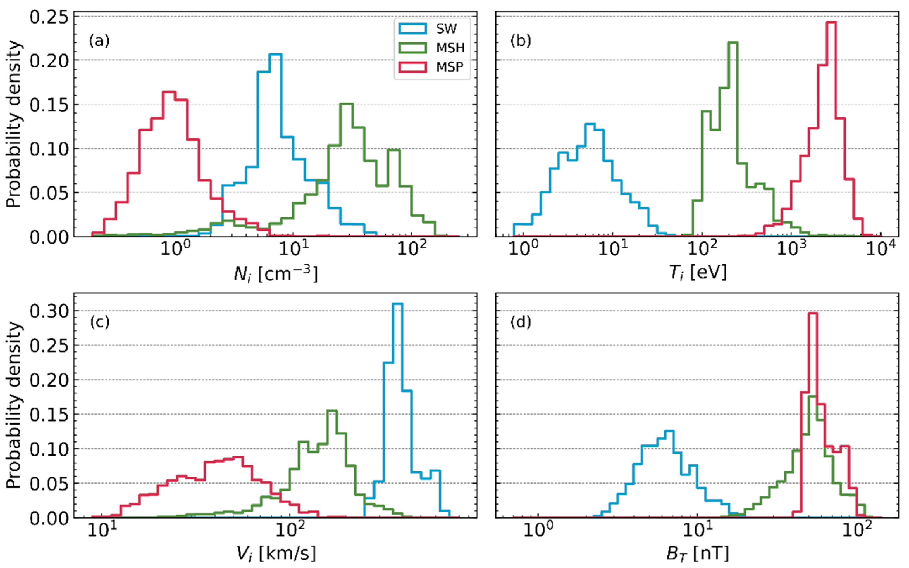
Figure 2 illustrates the probability density distributions of four key plasma parameters: proton density (n_p), proton temperature (T_p), bulk velocity (V_p), and total magnetic field strength (B_T) across three distinct regions: the solar wind, the magnetosheath, and the magnetosphere. The distribution of np reveals lower densities in the solar wind, peaking at a few particles per cubic centimeter, whereas higher densities are observed in the magnetosheath, reaching up to 100 cm⁻³. The magnetosphere exhibits relatively lower densities, typically less than 30 cm⁻³, consistent with the expected decrease in ion density from the solar wind to the magnetosphere. The proton temperature in the solar wind is lower, typically less than 100 eV, while the magnetosheath shows an intermediate range of 100–1000 eV. The magnetosphere, on the other hand, exhibits the highest temperatures, peaking between 1000 and 10,000 eV, in line with the expected increase in temperature from the solar wind to the magnetosphere. Proton bulk velocity is dominated by high speeds in the solar wind, ranging from 100 km/s to 600 km/s. In contrast, the magnetosheath displays a broader distribution with lower velocities, typically between 10 km/s and 100 km/s. The magnetosphere, characterized by low velocities, generally has values less than 50 km/s. This velocity profile is consistent with the expected decline in velocity from the solar wind to the magnetosphere. Lastly, the magnetic field strength is weakest in the solar wind, typically less than 10 nT, and increases progressively as one moves into the magnetosheath and magnetosphere, where it can reach values of up to 100 nT. This increase in magnetic field strength is consistent with the expected compression of the magnetic field as it interacts with the Earth’s magnetosphere.

The tripartite distribution of plasma parameters across the solar wind, magnetosheath, and magnetosphere reveals fundamental plasma transformations occurring at key boundaries, exhibiting distinct trends in B, T, V, and n. The bow shock mediates this transition through several interconnected processes: as the supersonic solar wind encounters the shock, it undergoes substantial deceleration and compression, converting kinetic energy into thermal energy. This results in (1) decreased bulk velocity V due to kinetic energy dissipation, (2) enhanced magnetic field strength B and plasma density n through compression, and (3) increased temperature T as the plasma is thermalized. Downstream of the bow shock, the magnetopause establishes a dynamic boundary separating the shocked solar wind plasma of the magnetosheath from Earth’s magnetosphere. Within the magnetosphere, the magnetic field becomes dominated by Earth’s intrinsic dipole field, typically exceeding the IMF strength by an order of magnitude. Here, ions become frozen into the geomagnetic field lines, with their convection governed by the large-scale magnetospheric/convective electric field.

The accurate classification of plasma regions poses significant challenges due to overlapping parameter distributions across different domains. Traditional threshold-based approaches [23,24] often prove inadequate for precise boundary layer identification, particularly during bow shock and magnetopause crossings, as they cannot account for dynamic solar wind interactions. While high-resolution, multi-parameter observations are recognized as essential for resolving boundary layer structures [25], conventional methods still struggle with ambiguous parameter ranges in transitional regions like the magnetosheath–magnetopause interface. These limitations become particularly evident during extreme solar wind conditions, where empirical models frequently disagree with in situ satellite measurements [26]. To overcome these limitations, WDTC has been developed as a promising solution. This model combines the robust classification capabilities of decision trees with the wavelet transform’s ability to capture and analyze temporal fluctuations in the time-frequency domain. By integrating these strengths, the WDTC effectively navigates the dynamic and complex nature of boundary layer transitions, making it a powerful tool for identifying bow shock and magnetopause structures within large satellite datasets.

3. Labeled Dataset

3.1. Data Interpretation

The data used in this study were sourced from NASA’s MMS mission, as detailed by [27]. The MMS mission consists of a fleet of four satellites designed to investigate the dynamic processes underlying the interaction between Earth’s magnetosphere and the solar wind, with a particular focus on magnetic reconnection. The dataset includes a range of physical parameters recorded across different spatial locations, such as plasma density, velocity, magnetic field intensity, and electron temperature.

Magnetic field measurements from the MMS constellation were obtained using the Fluxgate Magnetometer (FGM) instrument, as described by [28]. The FGM operates in two distinct data modes: a high-time-resolution mode that samples up to 128 Hz, and a lower-time-resolution mode at 8 Hz. Plasma data were primarily gathered using the Fast Plasma Investigation (FPI) instrument, as reported by [29]. The FPI provides several time-resolution modes, measuring the ion and electron distribution functions and calculating the moments of those distributions with cadences of 150 ms and 30 ms, respectively. In the MMS region of interest, the FPI typically operates in Fast Survey mode, with data taken at burst resolution (30 ms for the electron distribution and 150 ms for the ion distribution). Additionally, data are available at survey resolution (e.g., 4.5 s). For the purposes of this study, we utilized the lower-resolution data of 0.125 s and 4.5 s from both the FGM and FPI instruments.

For data processing, magnetic field and plasma measurements from the MMS1 satellite were extracted from the MMS Science Data Center. The dataset was filtered to focus on the period from 10 September to 31 December 2015. The Geocentric Solar Ecliptic (GSE) coordinate system was employed for the analysis, providing a consistent framework for interpreting spatial data.

3.2. Data Preprocessing

Given the varying sampling rates of the instruments aboard the MMS satellites, comprehensive data cleaning and preprocessing were essential to ensure the uniformity and accuracy of the dataset. The first step involved data alignment, which was carried out to meet the specific requirements of MMS data analysis. To preserve the high temporal resolution of the magnetic field data, a “low-to-high” data alignment technique was employed. This technique aligned all ion-related data, such as ion velocity, density, and temperature, onto the same time axis as the magnetic field data, ensuring consistency in the temporal reference. As a result, the entire dataset was standardized to a uniform time resolution of 0.125 s, matching the native sampling rate of the FGM measurements.

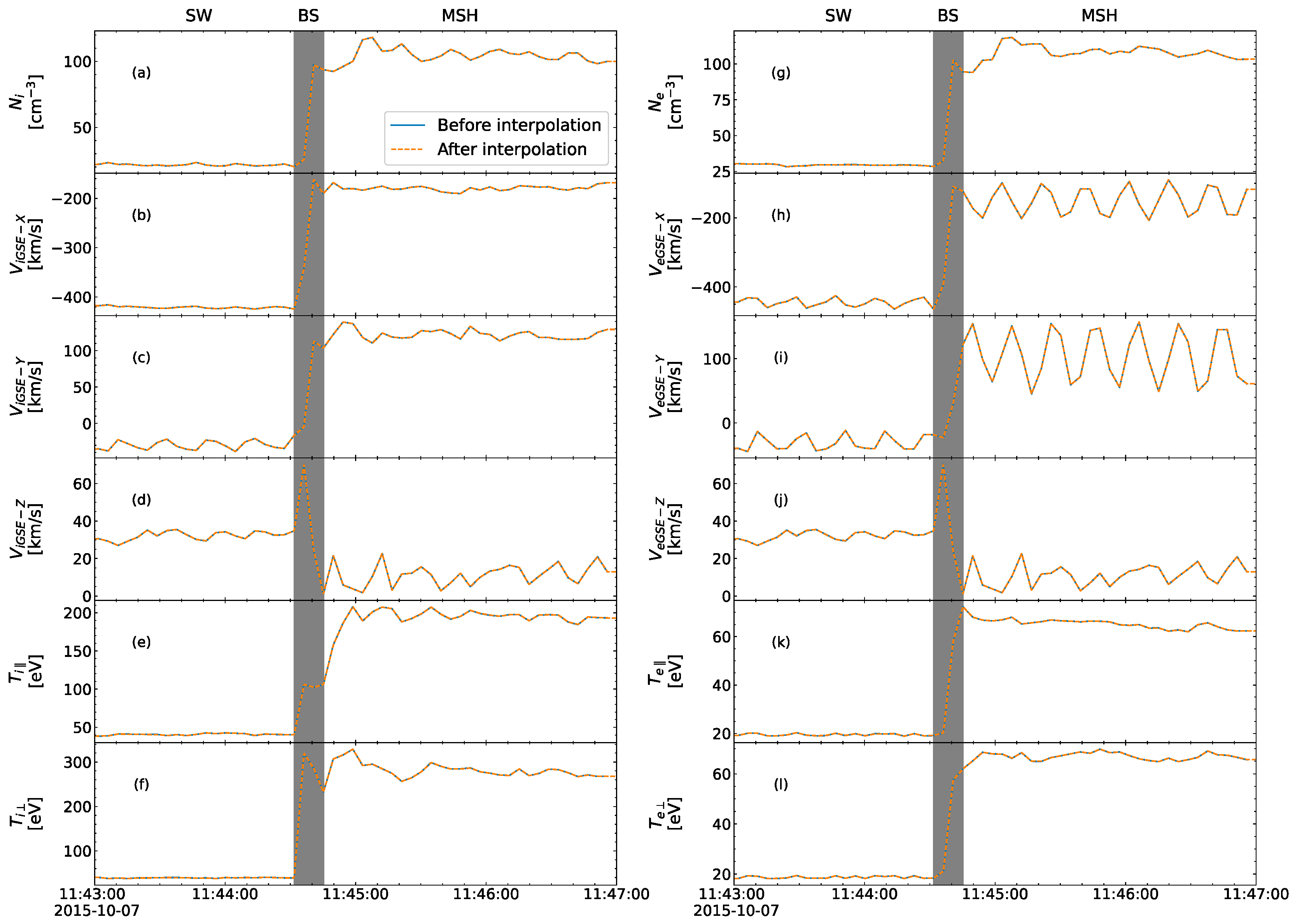
To validate the robustness of our interpolation methodology, Figure 3 presents a comprehensive comparison between original and interpolated plasma parameters during a turbulent bow shock crossing event observed by MMS on 7 October 2015 (11:43:00–11:47:00 UTC). Systematic analysis of ion and electron dynamics across bow shock reveals excellent agreement, with ion velocities showing mean absolute errors (MAEs) of 1.22 × 10⁻⁵ (SW), 1.12 × 10⁻³ (BS), and 6.22 × 10⁻⁵ (MSH), while electron velocities exhibit slightly higher but still exceptional consistency (1.60 × 10⁻⁴ SW, 3.68 × 10⁻³ BS, 1.19 × 10⁻³ MSH). Maximum deviations occur at the bow shock transition (1.66 × 10⁻³ for ions, 8.43 × 10⁻³ for electrons), where plasma conditions are most dynamic. The interpolation precisely reproduces both gradual solar wind variations and abrupt magnetosheath transitions, capturing characteristic density spikes (e.g., at 11:44:45) with errors of 8.62 × 10⁻³ (ions) and 6.84 × 10⁻³ (electrons). Temperature components maintain particularly strong fidelity (MAE: 2.87 × 10⁻⁴ for ions, 1.72 × 10⁻⁴ for electrons), accurately preserving the development of temperature anisotropy behind the shock front. Notably, errors in the solar wind remain consistently an order of magnitude lower than those at the bow shock, demonstrating the method’s ability to maintain accuracy across dramatically different plasma regimes while providing the uniform temporal resolution essential for quantitative analysis of MMS observations.

3.3. Labeled Dataset Generation

Manual labeling of event samples is a cornerstone in creating a dataset suitable for training and validating machine learning models. For this study, the dataset includes experimentally measured physical quantities such as magnetic field (B), ion velocity components (V), ion density (n), and ion temperature (T). The dataset is organized into five plasma region categories: bow shock, magnetosheath, solar wind, magnetopause, and magnetosphere. Each category contains 100 samples, resulting in a total of 500 data samples, as summarized in

Table 1. Sample distribution for each plasma region in the labeled dataset.

PRC	Total Samples	Typical Samples	Ordinary Samples	Proportion of Typical Samples
BS	100	98	2	98%
MP	100	98	2	98%
SW	100	94	6	94%
MSH	100	95	5	95%
MSP	100	96	4	96%

Note: PRC represents the plasma region category (e.g., BS = bow shock, MP = magnetopause, MSH = magnetosheath, SW = solar wind, MSP = magnetospheric boundary).

.

Based on the intensity of wave and/or turbulence activity, the samples are categorized into two groups: “typical” and “ordinary”. Typical samples are characterized by weak to moderate wave/turbulence activity, while ordinary samples display strong wave/turbulence activity. This distinction provides a more nuanced understanding of the plasma regions and their dynamic behavior, which is essential for accurately classifying plasma events using machine learning.

The final labeled dataset includes data collected from 2015 to 2017, ensuring a comprehensive range of plasma conditions and boundary layer events for model training and evaluation. Given that boundary layer crossing times typically range from 30 to 60 s, we selected 60 s time series for samples of the BS and MP. For events not involving boundary layers, such as the solar wind and magnetosheath, we opted for 4 min time series to ensure adequate coverage and preserve the integrity of the feature readings.

The labeling process began with the manual annotation of a smaller subset of the data, which was then used to train an initial version of the machine learning model. After training the initial model, its predictions were leveraged to assist in the labeling of additional data, allowing the labeled dataset to expand incrementally. This iterative approach continued until the dataset reached the target size, as outlined in the paper. The labeling process itself was conducted through visual inspection of the data, with the preliminary model’s predictions serving to expedite the annotation process.

4. Wavelet Decision Tree Classifier Model

The decision tree model is a robust, non-parametric supervised learning method, well-regarded for its ability to handle complex, non-linear relationships within feature data. In this study, we employed the WDTC model for both plasma region classification and boundary layer identification.

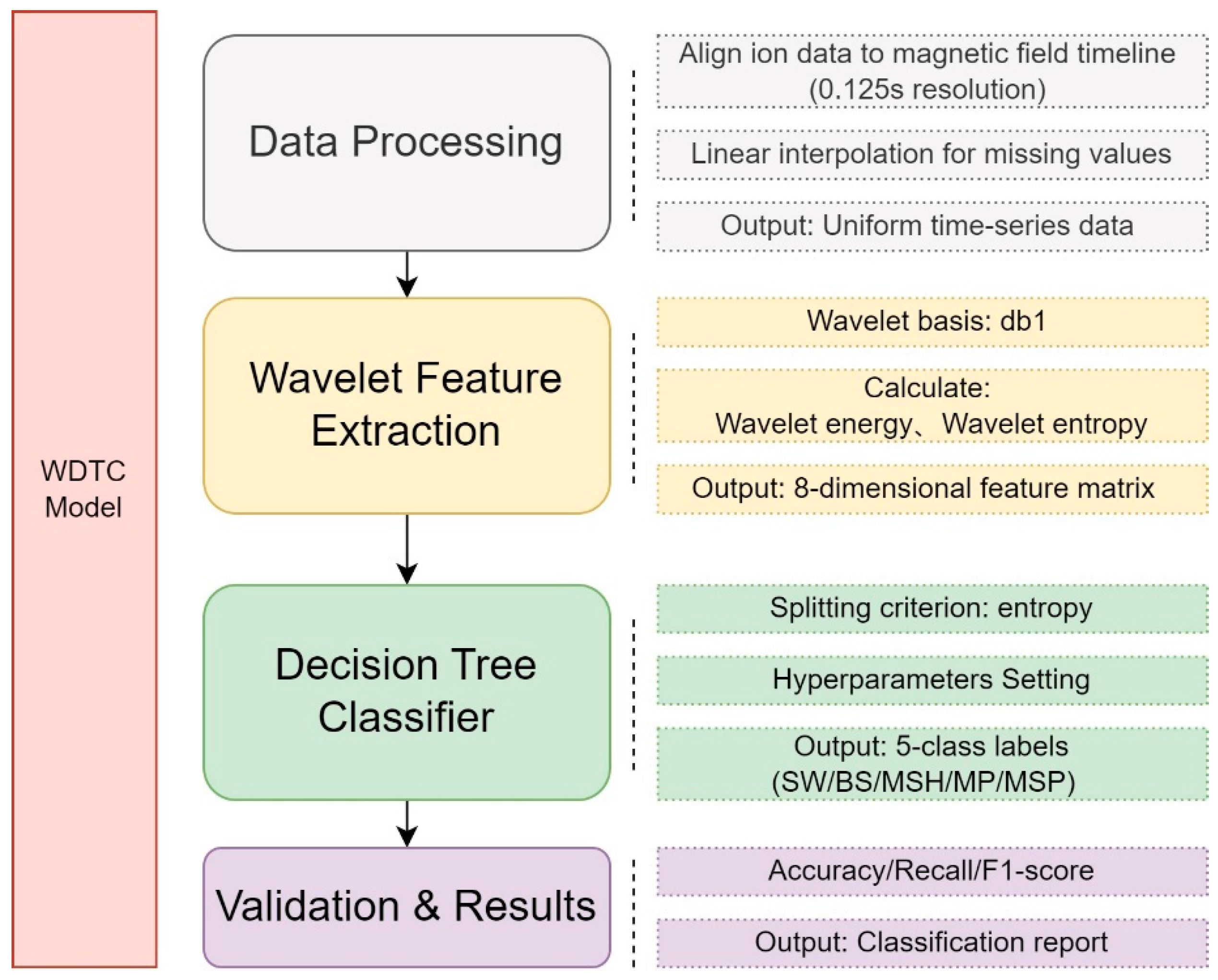
Figure 4 illustrates the WDTC pipeline, providing a clear overview of the classification process. As shown in Figure 4, the WDTC pipeline begins by synchronizing ion data with high-resolution (0.125 s) magnetic field measurements, employing linear interpolation to ensure continuity in the time-series data. Next, discrete wavelet transforms (db1 basis) decompose the signals to extract an eight-dimensional feature matrix, comprising wavelet energy and entropy metrics that encode multiscale plasma dynamics. These features train a decision tree classifier with entropy-based splitting, enabling classification into five critical plasma regions: solar wind, bow shock, magnetosheath, magnetopause, and magnetosphere. Model performance is evaluated using standard metrics (accuracy, recall, F1 score), with results summarized in a classification report.

4.1. Wavelet Tool

For this study, we selected the db1 wavelet from the Daubechies wavelet family as our primary wavelet tool. The db1 wavelet was applied to each time series to perform wavelet decomposition, which breaks down the signals into four distinct levels of decomposition. The wavelet tool generates wavelet energy, a key measure of the signal’s amplitude strength across the time series. The wavelet energy is computed using the following formula:

$$\mathrm{e}\mathrm{n}\mathrm{e}\mathrm{r}\mathrm{g}\mathrm{y}=\sum \left({\mathrm{C}}^2\right)$$

(1)

where C represents the wavelet coefficients. This energy measure is vital for understanding the variations in signal strength over time, contributing to the accurate classification of plasma regions and boundary layers.

Below, we detail the roles of the wavelet transform and decision tree classifier in the WDTC framework.

Furthermore, the wavelet tool outputs wavelet entropy, a measure of the signal’s complexity. By calculating the energy proportion of each wavelet coefficient of the normalized value P $={\displaystyle \frac{{\mathrm{C}}^2}{\mathrm{E}\mathrm{n}\mathrm{e}\mathrm{r}\mathrm{g}\mathrm{y}}}$. The entropy value is computed using Shannon’s entropy formula. The entropy for each frequency band is calculated by:

$$\mathrm{e}\mathrm{n}\mathrm{t}\mathrm{r}\mathrm{o}\mathrm{p}\mathrm{y}\left(\mathrm{k}\right)=-\sum (\mathrm{P}\cdot \mathrm{l}\mathrm{o}\mathrm{g}(\mathrm{P}+\mathsf{\epsilon }\left)\right)$$

(2)

The ε term defines the minimum allowable value for the normalized energy proportion P = C²/Energy as it asymptotically approaches zero, ensuring the preservation of the logarithmic term’s definiteness (P + ε > 0).

An increase in wavelet entropy typically signifies a higher level of chaos or irregularity in the signal. When wavelet entropy is elevated, it suggests that the signal encompasses a wider range of frequency bands within the sequence, indicating greater complexity. In the context of shock wave and magnetopause crossing regions, wavelet entropy aids in identifying points of sudden changes in the signal.

Table 2. Wavelet energy and wavelet entropy of 4 parameters extracted from time series corresponding to different categories.

Start Time	Dur (min)	B_WE (nT)2	B_E	V_WE (km/s)2	V_E	n_WE (cm−3)2	n_E	T_WE (eV)2	T_E	PRC
15 October 2017 05:32	1	1.07 × 105	3.862	1.86 × 108	4.05	6.1 × 104	3.73	1.91 × 108	4.03	BS
22 January 2016 23:03	1	1.9 × 106	4.083	1.02 × 107	4.05	7.0 × 103	3.48	3.37 × 108	4.07	MP
21 October 2015 11:02	4	6.0 × 106	5.468	7.49 × 107	5.47	2.0 × 106	5.46	1.98 × 108	5.47	MSH
7 October 2015 12:13	4	9.0 × 105	5.478	6.46 × 108	5.48	1.9 × 106	5.47	4.80 × 106	5.48	SW
6 February 2016 05:47	4	1.3 × 107	5.477	1.66 × 106	4.90	1.3 × 103	5.47	4.17 × 109	5.47	MSP

Note: B_WE, V_WE, n_WE, and T_WE represent the wavelet energy of the magnetic field, velocity, particle number density, and temperature, respectively. B_E, V_E, n_E, and T_E represent the corresponding wavelet entropy values.

presents wavelet energy (_WE) and wavelet entropy (_E) values for four critical plasma parameters extracted from time series data corresponding to various plasma regions. The wavelet energy values of the magnetic field strength (B_WE) indicate the highest variability in the magnetopause region, where the B_WE value reaches 1.3 × 10⁷ during the event on 6 February 2016. This is consistent with the magnetopause being a dynamic boundary layer, characterized by significant magnetic field fluctuations resulting from the interaction between the solar wind and the magnetosphere. In contrast, the bow shock on 15 Octorbar 2017 shows a relatively lower B_WE value of 1.07 × 10⁵, suggesting that while the bow shock is a transition region, its magnetic field fluctuations are less intense compared to the magnetopause. The wavelet energy of ion velocity (V_WE) also shows notable variation across the plasma regions. The highest V_WE is observed in the magnetosheath, with a value of 7.5 × 10⁷ on 21 October 2015, indicating substantial fluctuations in ion velocity due to the compression and deceleration of the solar wind in the magnetosheath. The solar wind region, on the other hand, exhibits a significantly lower V_WE value of 6.46 × 10⁸ on 7 October 2015, reflecting the more uniform and steady flow of ion velocity within the solar wind.

Similarly, the ion density wavelet energy (n_WE) shows substantial variability across regions. The magnetosheath region exhibits the highest n_WE value (6.1 × 10⁴) on 21 October 2015, which corresponds to the higher ion density observed in this region due to the compression of solar wind particles. In contrast, the solar wind region shows a lower n_WE value of 2.0 × 10⁶ on 7 October 2015, reflecting the lower ion density found in the less dense solar wind. The ion temperature wavelet energy (T_WE) follows a similar trend, with the highest T_WE values found in the magnetosheath and magnetosphere, reflecting the thermal fluctuations in these regions. For instance, the magnetosheath region on 21 October 2015 exhibits a T_WE value of 4.80 × 10⁶, which corresponds to the increased ion temperature due to heating as the solar wind slows down and compresses.

From Table 2, the ion velocity and density both exhibit relatively higher entropy in the boundary regions (magnetopause and magnetosheath), suggesting more complex, multi-scale behavior in these areas due to the dynamic interactions between the solar wind and the magnetosphere. The entropy values for T and B generally follow similar trends, with the magnetosheath and magnetopause showing higher entropy, indicating a greater diversity of temporal scales in these regions compared to the more uniform conditions in the solar wind and magnetosphere.

These results demonstrate the utility of wavelet transform in capturing the complexity of plasma parameters across different regions of near-Earth space. The wavelet energy and entropy values provide detailed insight into the fluctuations and variability of plasma conditions, offering valuable information for the plasma region classification and boundary layers identification.

4.2. Decision Tree Model

In this study, we employed the decision tree classifier implemented in the Scikit-learn library, which autonomously identifies the most discriminative features for partitioning the data. This capability makes the decision tree particularly advantageous for analyzing signals characterized by a variety of frequency bands, such as those derived from wavelet transforms. By leveraging wavelet-derived features, the decision tree model effectively classifies signals from different plasma regions, including the solar wind, magnetosheath, magnetosphere, and boundary layers (such as the magnetopause and bow shock).

We chose decision tree models over neural networks due to their superior interpretability, computational efficiency, and better alignment with our dataset characteristics. While neural networks can model complex nonlinear relationships effectively, they typically require larger datasets and greater computational resources while offering limited interpretability. In contrast, decision trees provide clear, logical decision rules that satisfy our need for explainable results. Our moderate-sized dataset with well-defined feature boundaries proved particularly suitable for tree-based methods. The decision trees achieved accuracy comparable to neural networks while offering greater transparency and significantly lower computational overhead. This approach optimally balances predictive performance with practical requirements for interpretability and resource efficiency in our application.

When applying the decision tree in conjunction with wavelet transforms, we use an entropy-based splitting criterion. The model recursively partitions the dataset based on this criterion, with entropy which quantifies information gain, playing a key role in guiding the model to select the most informative feature at each split. This process of selecting the optimal feature at each node enhances the model’s ability to distinguish between different signal classes, thereby improving its classification accuracy.

The model hyperparameters were configured as follows to optimize plasma boundary detection:

• Splitting criterion: ‘entropy’ to maximize information gain at each node for effective feature discrimination.
• Minimum samples split: 2 (default) to preserve fine-scale plasma transitions without over-segmentation.
• Minimum samples leaf: 1 (default) to ensure sensitivity to subtle boundary features while maintaining robustness.
• Pruning: Default settings retained to prevent underfitting without manual intervention.

The db1 (Haar) wavelet was specifically chosen for its ability to resolve sharp transitions and high-frequency features characteristic of plasma boundaries. This selection, combined with our entropy-based splitting approach, ensures optimal detection of both gradual and abrupt boundary layer changes. All parameter choices were rigorously validated through iterative cross-validation experiments, demonstrating consistent performance across diverse plasma regimes. This configuration balances model complexity with predictive reliability, as evidenced by WDTC’s robust performance in our test cases.

4.3. Performance Evaluation

To evaluate the effectiveness of the classification model, we used several key metrics: accuracy, recall, F1 score, and Matthews correlation coefficient (MCC) [30]. These metrics are defined as follows:

True positive (TP): The number of positive samples correctly identified as positive by the model.

False positive (FP): The number of negative samples incorrectly identified as positive by the model.

False negative (FN): The number of positive samples incorrectly identified as negative by the model.

The performance metrics are calculated using the following formulas:

Accuracy is the proportion of correctly predicted positive samples out of all predictions made by the model:

$$\mathrm{A}\mathrm{c}\mathrm{c}\mathrm{u}\mathrm{r}\mathrm{a}\mathrm{c}\mathrm{y}={\displaystyle \frac{\mathrm{T}\mathrm{P}}{\mathrm{T}\mathrm{P}+\mathrm{F}\mathrm{P}}}$$

(3)

Recall, also known as sensitivity, measures the proportion of actual positives that were correctly identified:

$$\mathrm{R}\mathrm{e}\mathrm{c}\mathrm{a}\mathrm{l}\mathrm{l}={\displaystyle \frac{\mathrm{T}\mathrm{P}}{\mathrm{T}\mathrm{P}+\mathrm{F}\mathrm{N}}}$$

(4)

F1 score is the harmonic mean of precision and recall. Precision is the proportion of positive identifications that were actually correct:

$$\mathrm{F}1=2\times {\displaystyle \frac{\mathrm{P}\mathrm{r}\mathrm{e}\mathrm{c}\mathrm{i}\mathrm{s}\mathrm{i}\mathrm{o}\mathrm{n}\times \mathrm{R}\mathrm{e}\mathrm{c}\mathrm{a}\mathrm{l}\mathrm{l}}{\mathrm{P}\mathrm{r}\mathrm{e}\mathrm{c}\mathrm{i}\mathrm{s}\mathrm{i}\mathrm{o}\mathrm{n}+\mathrm{R}\mathrm{e}\mathrm{c}\mathrm{a}\mathrm{l}\mathrm{l}}}=2\times {\displaystyle \frac{\mathrm{T}\mathrm{P}}{2\mathrm{T}\mathrm{P}+\mathrm{F}\mathrm{P}+\mathrm{F}\mathrm{N}}}$$

(5)

To further assess the model’s performance, especially for multi-class classification, we also calculated macro average and weighted average metrics:

Macro average computes the average metric across all categories, treating each category equally regardless of its size:

$$\mathrm{M}\mathrm{a}\mathrm{c}\mathrm{r}\mathrm{o} \mathrm{A}\mathrm{v}\mathrm{e}\mathrm{r}\mathrm{a}\mathrm{g}\mathrm{e}={\displaystyle \frac{1}{\mathrm{C}}}{\sum }_{\mathrm{i}=1}^{\mathrm{C}}{\mathrm{M}\mathrm{e}\mathrm{t}\mathrm{r}\mathrm{i}\mathrm{c}}_{\mathrm{i}}$$

(6)

Weighted average adjusts the average metric according to the number of samples in each category. This is particularly useful when working with imbalanced datasets:

$$\mathrm{W}\mathrm{e}\mathrm{i}\mathrm{g}\mathrm{h}\mathrm{t}\mathrm{e}\mathrm{d} \mathrm{A}\mathrm{v}\mathrm{e}\mathrm{r}\mathrm{a}\mathrm{g}\mathrm{e}={\displaystyle \frac{1}{N}}{\sum }_{i=1}^C{N}_i\times {\mathrm{M}\mathrm{e}\mathrm{t}\mathrm{r}\mathrm{i}\mathrm{c}}_i$$

(7)

where C is the total number of categories in the classification task (in this study, C = 5), N_i is the number of samples in class I, and Metric_i is the specific metric (e.g., accuracy, recall, F1 score) for class i.

MCC gives a comprehensive classification assessment considering all prediction outcomes:

$$MCC={\displaystyle \frac{TP\times TN-FP\times FN}{\sqrt{(TP+FP)(TP+FN)(TN+FP)(TN+FN)}}}$$

(8)

where TN represents true negatives (with TP + TN + FP + FN = total number of samples).

5. Model Training

The dataset was randomly split into a training set, comprising 80% (400 samples) of the data, and a test set, which made up the remaining 20% (100 samples). The training set was utilized to train the decision tree model, while the test set was reserved to assess the model’s ability to generalize to unseen data. A total of 500 samples were input into the decision tree for the training process. Ten experiments were conducted by randomly changing the samples contained in the test set and the training set. To evaluate the model’s performance, the results are summarized in

Table 3. Performance evaluation of the WDTC in different plasma regions.

Region		Ex1	Ex2	Ex3	Ex4	Ex5	Ex6	Ex7	Ex8	Ex9	Ex10	Avg
BS	precision	1.00	0.95	0.90	1.00	1.00	1.00	0.89	1.00	1.00	0.90	0.96
	recall	1.00	0.95	0.95	0.92	1.00	0.91	0.94	0.94	0.85	1.00	0.95
	F1 score	1.00	0.95	0.92	0.96	1.00	0.95	0.92	0.97	0.92	0.95	0.95
MP	precision	0.96	0.94	1.00	1.00	1.00	0.92	1.00	0.94	1.00	1.00	0.98
	recall	1.00	1.00	1.00	1.00	0.96	1.00	1.00	0.94	1.00	0.94	0.98
	F1 score	0.98	0.97	1.00	1.00	0.98	0.96	1.00	0.94	1.00	0.97	0.98
MSH	precision	0.93	1.00	0.96	1.00	1.00	1.00	0.95	0.96	1.00	1.00	0.98
	recall	0.91	0.95	1.00	1.00	0.94	1.00	0.95	0.88	0.96	1.00	0.96
	F1 score	0.96	0.97	0.98	1.00	0.97	1.00	0.95	0.92	0.98	1.00	0.97
MSP	precision	1.00	0.91	0.94	0.92	0.94	0.89	0.95	0.91	0.98	0.95	0.94
	recall	0.95	0.91	0.88	1.00	1.00	0.89	0.90	1.00	1.00	0.90	0.94
	F1 score	0.98	0.91	0.91	0.96	0.97	0.89	0.92	0.95	0.93	0.93	0.94
SW	precision	1.00	1.00	1.00	1.00	0.94	1.00	0.96	0.90	0.94	1.00	0.97
	recall	0.96	1.00	0.94	1.00	1.00	1.00	0.96	0.92	1.00	1.00	0.98
	F1 score	0.98	1.00	0.97	1.00	0.97	1.00	0.96	0.95	0.97	1.00	0.98
Accuracy		0.98	0.96	0.96	0.98	0.98	0.96	0.95	0.94	0.96	0.97	0.96
Macro Avg	precision	0.98	0.96	0.96	0.98	0.96	0.96	0.95	0.96	0.97	0.97	0.97
	recall	0.98	0.96	0.95	0.98	0.96	0.96	0.95	0.96	0.97	0.97	0.96
	F1 score	0.98	0.96	0.96	0.98	0.96	0.96	0.95	0.96	0.97	0.97	0.97
Weighted Avg	precision	0.98	0.96	0.96	0.98	0.96	0.96	0.95	0.96	0.97	0.97	0.97
	recall	0.98	0.96	0.96	0.98	0.96	0.96	0.95	0.96	0.97	0.97	0.97
	F1 score	0.98	0.96	0.96	0.98	0.96	0.96	0.95	0.96	0.97	0.97	0.97

below.

Results presented in Table 3 highlight the model’s overall performance across various plasma regions. For the bow shock region, the WDTC showed impressive results, with precision values consistently close to 1.00, indicating that the model was highly accurate in identifying BS events. The recall values were also strong, particularly in experiments 1, 4, and 5, where the recall was 1.00, suggesting that the model was able to successfully capture almost all BS events. The F1 score for BS was calculated to have an average of 0.95, demonstrating a good balance between precision and recall.

For the magnetopause region, the precision values were similarly high, averaging around 0.96, indicating that the WDTC effectively distinguished MP events from other plasma regions. However, the recall for MP was slightly lower than that for BS, averaging around 0.91. This suggests that, although the model was generally accurate, it may have missed some MP events, which is reflected in the lower recall values. The F1 scores for MP remained solid, with an average value of 0.94, signifying that the model’s performance was balanced and reliable in classifying MP events.

The solar wind and magnetosheath regions also exhibited strong performance metrics, with the precision and recall values reflecting the model’s ability to classify these regions accurately. Across 10 repeated experiments, the model exhibits stable performance (accuracy = 96.4%, σ = 1.2%), confirming that variability is well controlled. While there were slight variations in recall across the experiments, the overall performance remained consistent. The average F1 scores for these regions were also high, further confirming the effectiveness of the WDTC in classifying plasma events. The averaged MCC (Matthews correlation coefficient) value is 0.96, which indicates excellent classification performance, demonstrating strong robustness to class imbalance and minimal false positive/negative rates.

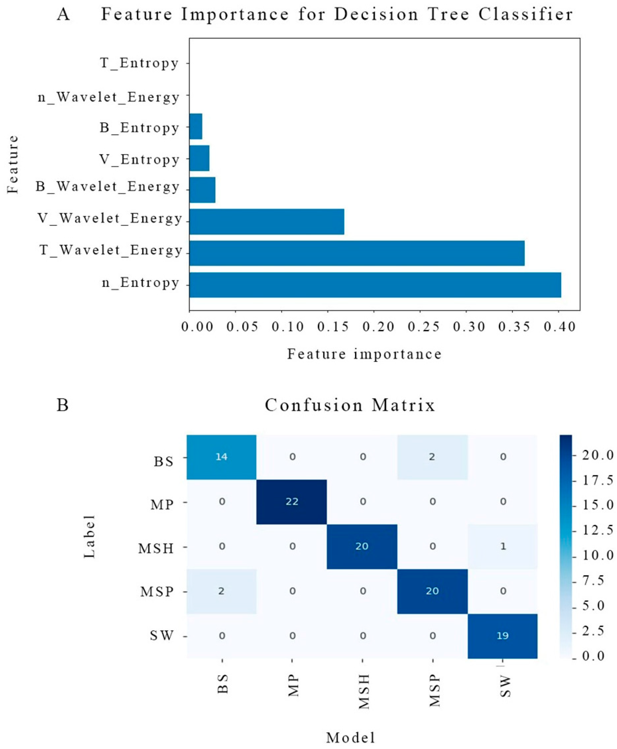
Subsequently, an additional experiment was performed to analyze feature importance using the decision tree classifier. Figure 5A illustrates the feature importance values for the decision tree classifier, showing how each feature contributes to the classification process. The feature importance is calculated based on the ability of each feature to reduce the impurity of the decision tree nodes, with higher values indicating a greater contribution to the classification task. In this analysis, the feature “n_Entropy” stands out as the most significant, exhibiting the highest feature importance value, approaching 0.4. This suggests that n_Entropy plays a crucial role in distinguishing between different plasma regions and is the primary driver of the decision tree’s classification performance. Following n_Entropy, “T_Wavelet_Energy” emerges as the second most important feature, demonstrating its substantial influence in the classification process. Features such as “T_Entropy” and “B_Entropy” exhibit much lower importance, around 0.05 or less, indicating that these features contribute less to the decision-making process.

Figure 5B presents a confusion matrix that visually assesses the decision tree classifier’s performance across different space weather regions. In the BS region, the classifier correctly identified 14 out of 16 instances as bow shock, with only 2 instances misclassified as SW, demonstrating a high accuracy for this category despite the minor misclassifications. The MP category achieved perfect classification, with all 22 instances correctly predicted as magnetopause, reflecting the model’s excellent performance for this region. Similarly, the MSH region showed strong results, with 20 out of 23 instances correctly identified.

However, as the classifier is tested across additional regions, slight variations in performance are observed, with some categories showing minor misclassifications. These results demonstrate the model’s overall effectiveness in correctly classifying the different plasma regions, while also highlighting areas where further improvements could be made.

From Figure 6A, the receiver operating characteristic (ROC) curve analysis reveals the performance of the WDTC across various space weather regions. The bow shock region achieves a high area under the curve (AUC) value of 0.93, indicating strong performance with a high true positive rate (TPR) and relatively low false positive rate (FPR). The magnetopause region exhibits an exceptional AUC of 1.00, which indicates perfect classification—no misclassifications occur, and the model can flawlessly distinguish magnetopause events from others. Similarly, the magnetosheath category demonstrates an AUC of 0.98, reflecting a highly effective classification model that accurately identifies most instances with only a few potential misclassifications. The solar wind category follows closely, attaining an AUC of 0.99, which also signifies a near-perfect classification performance. The black dashed line in the figure represents the baseline scenario of random guessing, where the AUC equals 0.5, implying no discriminative power between the positive and negative classes. The fact that all of the class curves lie well above this line demonstrates that the WDTC model outperforms random guessing across all regions, successfully distinguishing different plasma regions and boundary layers based on the extracted features.

Figure 6B shows the complexity curve of the WDTC model, as determined by the maximum depth (max depth). Initially, as the max depth increases, the training accuracy rises sharply, quickly approaching a value of 1.0 at around a max depth of approximately 2.5. Beyond this point, the training accuracy plateaus, remaining at a high level. This sharp increase in training accuracy indicates that the model fits the training data well as its complexity increases, capturing more detailed patterns and relationships.

In contrast, the test accuracy exhibits a distinct behavior. Initially, it increases alongside training accuracy as the maximum depth grows, peaking between depths of 2.5 and 5. However, beyond this point, the test accuracy fluctuates and eventually stabilizes around 0.95. This suggests that while the model benefits from increased complexity at first, its ability to generalize (reflected in the test accuracy) reaches a plateau after a certain level of complexity. The growing gap between training and test accuracies signals the potential onset of overfitting. When the model becomes overly complex (e.g., as the maximum depth exceeds 5), it may begin to memorize the training data, excelling in training performance but struggling to generalize to new, unseen data.

6. Category Results

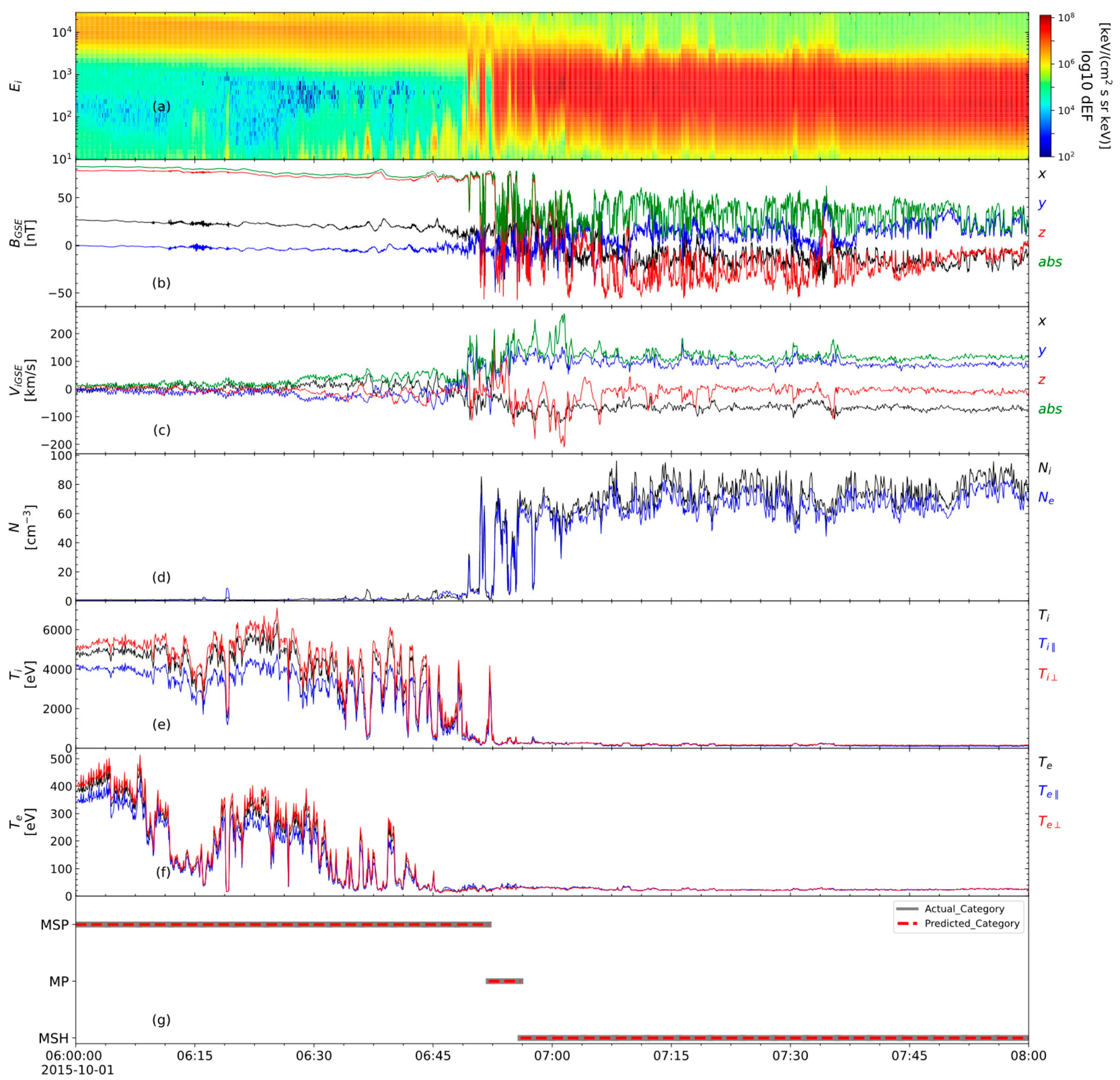
Figure 7 provides an in-depth visualization of the classification results as determined by the WDTC model using data from the MMS1 spacecraft on 1 October 2015. As illustrated in Figure 7e, the ion temperature T_i in the magnetosphere is significantly high, exceeding 5 keV. Moving toward the magnetopause, T_i gradually decreases before dropping sharply to several hundred eV upon entry into the magnetosheath. The electron temperature T_e, shown in Figure 7f, exhibits a similar trend but remains approximately an order of magnitude lower than T_i. In the magnetosphere, notable fluctuations in both T_i and T_e are observed, indicating dynamic activity and variations in thermal properties. Conversely, the magnetosheath is marked by significant variations in B and n, reflecting its role as a transitional zone where the solar wind interacts with the Earth’s magnetic field. The region near the magnetopause is characterized by strong turbulence in the velocity field V, which serves as a clear indicator of the boundary between the magnetosheath and the magnetosphere.

Figure 7g presents a comparison between the predicted category labels (represented by the red dashed lines) and the actual category labels (depicted by the grey solid lines). The black line in this panel denotes the actual category transitions inferred from the MMS data, providing a baseline for evaluation. The red line represents the predicted categories produced by the WDTC model. A close inspection of this panel reveals the high precision of the model in predicting the transitions between the MSP, MP, and MSH regions. The alignment of the red and black lines is nearly perfect, which indicates that the WDTC model successfully captures the magnetopause between these key plasma regions.

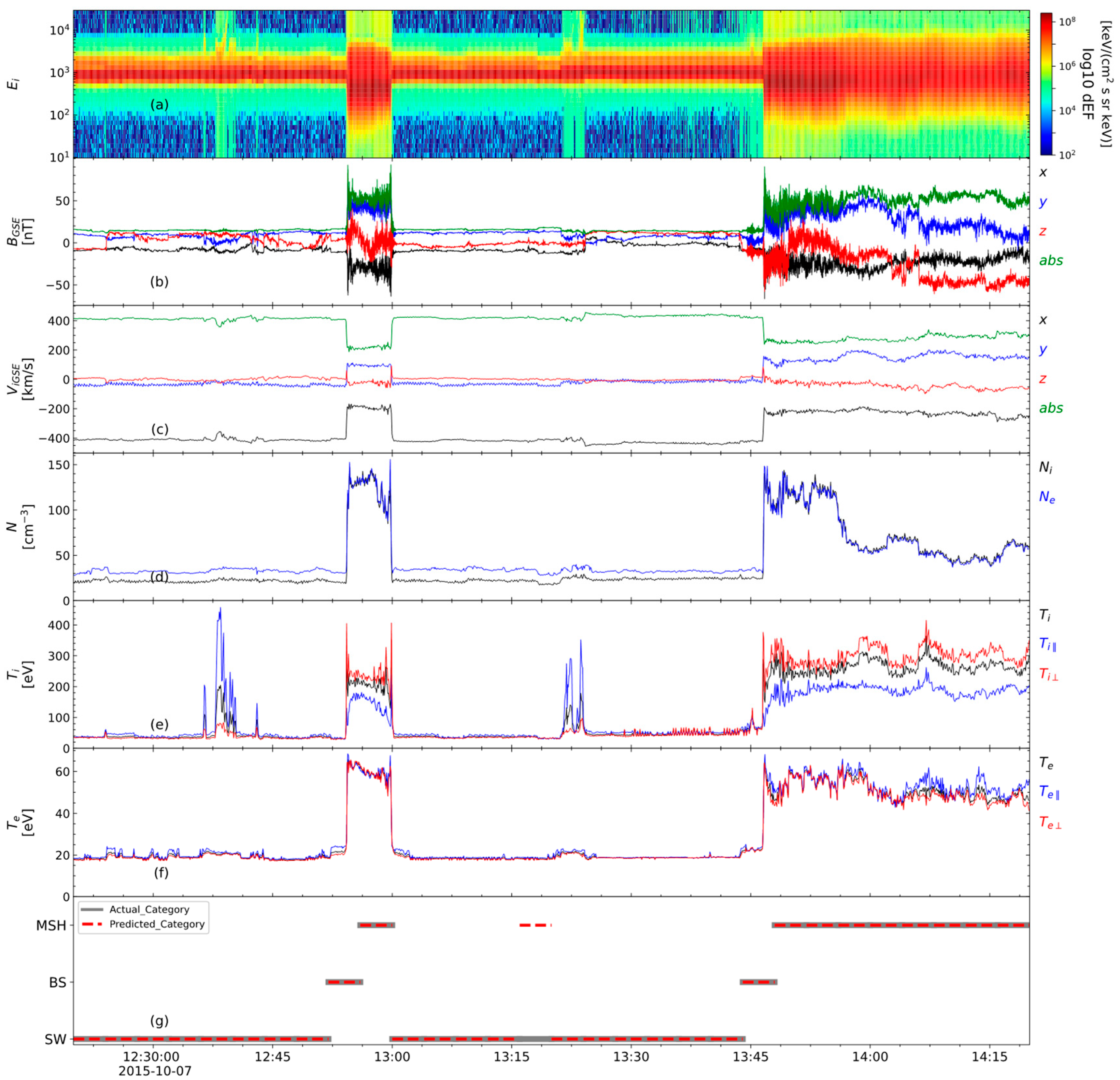
Figure 8 presents the classification results of the WDTC model for the solar wind, magnetosheath, and bow shock transitions, based on plasma parameter data collected on 7 October 2015. The model demonstrates high precision in identifying the SW region, which is characterized by high flow velocities, low ion densities, and cooler temperatures. The strong alignment between predicted and actual classifications in the SW region underscores the model’s effectiveness in accurately classifying the solar wind, whose distinctive features are clearly defined. Similarly, the WDTC model performs well in the MSH region, with a close correspondence between predicted and actual classifications (see Figure 8g).

Notably, the model faces challenges when classifying a specific plasma bubble event between 13:20 and 13:25, characterized by increased ion density and temperature (thermal pressure) along with a decrease in magnetic field strength (magnetic pressure). During this event, the WDTC misidentifies the plasma bubble as a BS transition. This misclassification is evident in the velocity data, where the plasma bubble exhibits a significantly lower speed compared to the solar wind. It is important to note that this misclassification is an isolated incident, occurring only once throughout the entire 2015 MMS dataset. Our analysis reveals that misclassifications primarily occur when transient plasma structures (e.g., solar wind plasma bubbles or shock transitions) exhibit wavelet-transformed signatures that closely resemble those of boundary layers. This feature space overlap creates inherent classification challenges, particularly when certain dynamic structures generate comparable wavelet energy/entropy patterns (15–20% overlap in principal components space).

Overall, the WDTC model demonstrates strong performance in classifying major plasma regions, including the solar wind, magnetosheath, and magnetopause, as well as boundary layer regions such as the bow shock and magnetopause. However, further refinements to the model could enhance its ability to accurately identify and distinguish transient events, ensuring even more precise classifications across diverse plasma and magnetic structures.

7. Discussion

7.1. Wavelet Transform vs. FFT

To compare with the wavelet transform, we trained the Fast Fourier Transform (FFT) on three plasma regions: the bow shock, solar wind, and magnetosheath. The experimental setup for FFT, including the sliding window size and sampling rate, was kept consistent with the settings used for the wavelet transform. To mitigate the effects of high-frequency noise, a Butterworth low-pass filter was applied to remove high-frequency components, with the cutoff frequency set at 10% of the sampling frequency.

The signal was segmented into multiple overlapping windows, each having a duration of 3 min (as determined by the sampling frequency). The overlap between adjacent windows was set to 50% of the window length to maintain continuity in the signal. FFT was applied to each window to obtain the amplitude spectrum in the frequency domain. For every window, we calculated the frequency components and extracted the dominant frequency, peak amplitude, and average spectrum value. The FFT analysis was performed using a pre-designed function, and a Hanning window was applied to the signal to minimize spectral leakage.

From the frequency spectrum of each window, the dominant frequency (i.e., the frequency with the highest amplitude) was selected, and both its value and corresponding amplitude were recorded. Additionally, we computed the average value of the signal within each window, which was then used as a feature input for the subsequent classification and pattern recognition tasks.

In the decision tree model used for the FFT transformation method, post-processing rules based on physical quantities were introduced to refine the model’s predictions. These rules were specifically designed to adjust the decision tree’s classifications by applying physical thresholds derived from the plasma parameters.

For bow shock classification, if the model predicts a category as the bow shock, the prediction remains unchanged. However, for non-bow shock regions, the classification is adjusted in accordance with the physical thresholds presented in

Table 4. Threshold range applied to different plasma region classifications.

	B (nT)	V (km/s)	n (/cm3)	T (eV)
SW	1–50	> 250	1–30	1–500
MSH	10–100	50–250	20–100	200–2000
BS	>20	<300	>10	>200

. These thresholds were chosen based on statistical analysis and are intended to complement the decision tree model, addressing its limitations in complex physical environments.

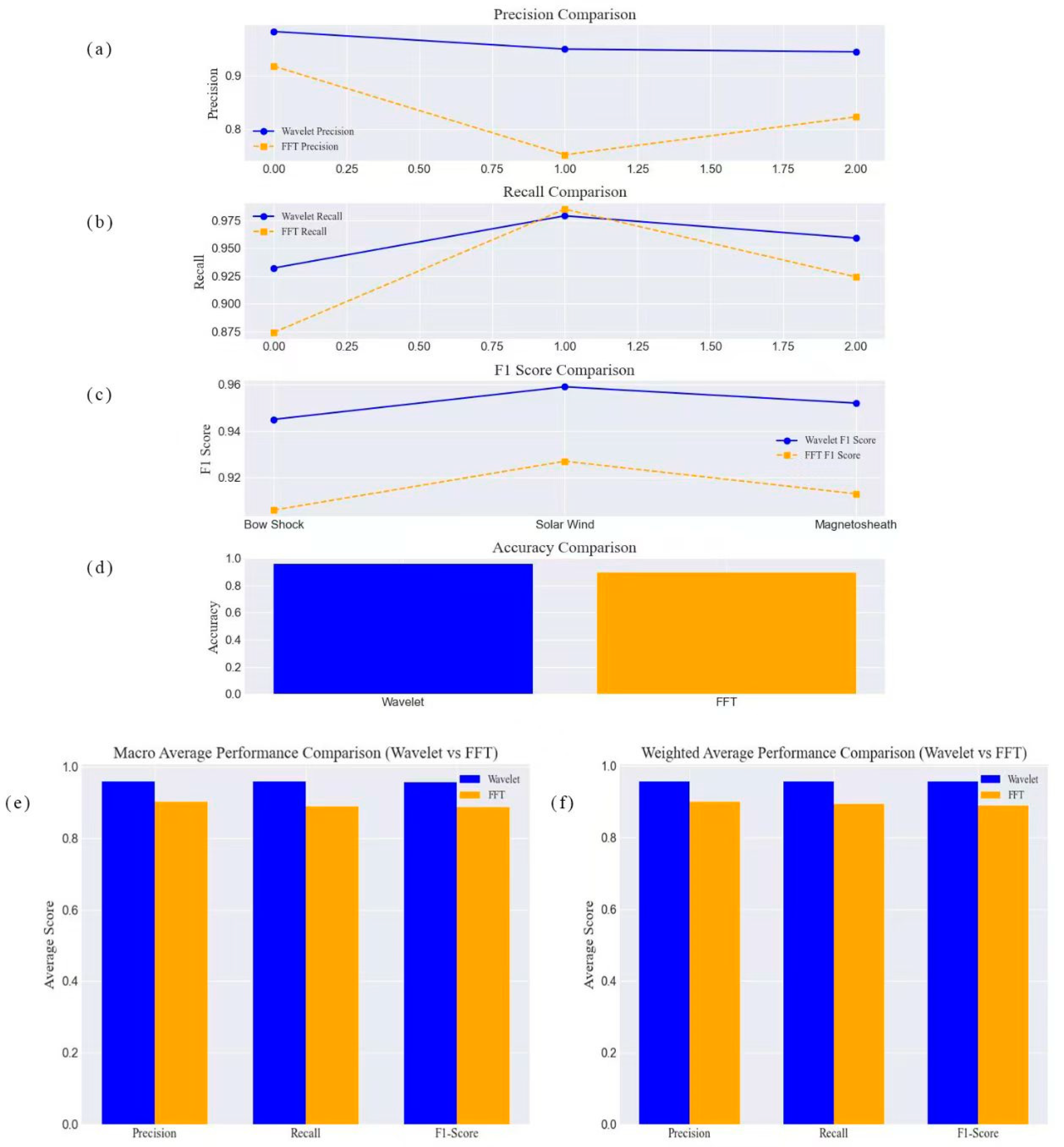
The final classification results were obtained by performing 10 random tests for each approach (wavelet transform and FFT). The average results from these tests were then computed to provide a robust evaluation of each method’s performance. The result is shown in Figure 9. For accuracy (in Figure 9a), in both the bow shock and magnetosheath categories, the average accuracy of the wavelet transform decision tree outperforms that of the FFT transform decision tree. For example, in the bow shock category, the accuracy for the wavelet transform is 0.983, while the average accuracy for the FFT transform is 0.918. In the magnetosheath category, the wavelet transform achieves an accuracy of 0.945, compared to 0.906 for the FFT transform. These findings suggest that the wavelet transform is more effective in accurately identifying samples in these regions.

For recall, in the solar wind category, the average recall for the FFT transform slightly exceeds that of the wavelet transform (0.985 vs. 0.979), indicating that the FFT transform is more successful in capturing all positive samples within this category. However, in other categories, the wavelet transform generally exhibits higher recall rates, showcasing its superior ability to detect positive instances in the magnetosheath and bow shock regions.

For F1 score, the wavelet transform consistently outperforms, or at least matches, the FFT transform in terms of F1 score across all categories, reflecting a more balanced classification performance. In the magnetosheath category, for instance, the wavelet transform achieves an average F1 score of 0.952, while the FFT transform achieves an average F1 score of 0.913. This emphasizes the wavelet transform’s superior overall performance, particularly in maintaining an optimal balance between precision and recall.

Specifically, In terms of macro average and weighted average, the precision, recall, and F1 scores of the wavelet transform are slightly higher than those of the FFT transform, further validating its stability and reliability across different categories. Specifically, the macro average F1 score of the wavelet transform is 0.956, while the macro average F1 score of the FFT transform is 0.887. The weighted average results exhibit a similar trend.

Overall, the wavelet transform consistently delivers superior classification results, particularly in the magnetosheath and bow shock regions, while also showing more balanced performance across multiple metrics. These findings underscore the advantage of the wavelet transform over FFT in this context, making it a more reliable method for identifying boundary layers.

7.2. Comparative Analysis: Wavelet-Decision Tree Model Versus Gaussian Mixture Model

In the comparative analysis, the WDTC model demonstrates a notable ability to identify the magnetosheath category, achieving a success rate of 66.2%. The aggregate true positive rate for the WDTC model stands at 95.5%, encompassing 16,972 cases, which includes the magnetosphere category at 28.2% and the solar wind category at 1.1%. Nevertheless, there are instances where the WDTC model’s classifications do not concur with the labels assigned by the GMM model, resulting in categorization as “False”.

The data presented in

Table 5. Comparative performance of WDTC and GMM models.

Compare		Category	Rate (%)	Total Rate (Count)
True Positive		MSH	66.2	95.5% (16,972)
		MSP	28.2
		SW	1.1
False	Positive	True BL	1.52	4.5% (788)
	Negative	False region	1.35
		False BL
		Bad BL	1.63

Note: ‘True’ indicates agreement with the common labels in our category and those of Toy-Edens et al. (2024) [20]. ‘False’ denotes discrepancies between the WDTC and GMM labels, where ‘True BL’ represents boundary layer cases correctly identified by WDTC but not by GMM, ‘False Region’ refers to regions misclassified by WDTC, and ‘Bad BL’ signifies incorrect boundary layer labels due to data gaps. ‘Count’ refers to the 4 min segments categorized by WDTC.

indicate that the WDTC model incorrectly classifies true boundary layer (True BL) cases at a rate of 1.52%, which constitutes a significant portion of the false negative rate, totaling 4.5% (788 cases). Additionally, the WDTC model misidentifies regions as ‘False Region’ at a rate of 1.35%. The ‘False BL’ category encapsulates instances where the WDTC model inaccurately labels the boundary layer. Moreover, the ‘Bad BL’ category accounts for 1.63% of the cases, which are misclassified due to data gaps. Exclusion of these data-gap-affected cases results in a notable enhancement of the WDTC model’s accuracy, achieving an impressive 98.6%. This figure underscores the WDTC model’s robustness when data completeness is ensured.

In summary, the WDTC model’s fundamental advantage lies in its unified framework architecture, which contrasts sharply with the GMM’s sequential two-step approach. Whereas the GMM first classifies plasma regions and then separately identifies boundary layers—a process prone to error propagation and suboptimal task coordination—the WDTC integrates both tasks into a single cohesive framework. This unified approach enables simultaneous optimization of region classification and boundary layer detection through coupled probability estimation and a consistent distance metric, eliminating inconsistencies inherent in decoupled processing. Additionally, the WDTC leverages wavelet transforms to extract dynamic time-series features (e.g., wavelet energy and entropy), enhancing its ability to detect boundary layer transitions. In contrast, the GMM struggles with complex temporal dynamics, leading to higher misclassification rates, particularly in boundary layer identification.

7.3. Boundary Layer Identification Using the WDTC Model

The integration of wavelet analysis into the WDTC enables precise identification of boundary layers. Between 15 September and 31 December 2015, the WDTC successfully detected 711 boundary layer crossings. By using temperature as a discriminative feature, these boundary layers were further categorized into bow shock and magnetopause events. Applying a temperature threshold of 1 keV, the WDTC identified 295 events as bow shock crossings (T < 1 keV) and 416 events as magnetopause crossings (T > 1 keV).

For future model enhancements, we intend to integrate additional in situ measurements, such as total magnetic field strength and plasma temperature, as input parameters. This upgrade is designed to enable the direct identification of boundary layers, thereby reducing reliance on the temperature threshold method. By incorporating these improvements, the WDTC model could be extended to the atmospheric environment, which is also characterized by significant wave activity [31,32].

8. Conclusions

In conclusion, the WDTC offers a robust and efficient approach for the automatic identification of dynamic boundary layers in complex plasma environments. The quantitative evaluation reveals outstanding performance metrics: the model achieved a mean classification accuracy of 96.4% (±1.2% standard deviation) across ten independent validation runs, with precision and recall values consistently exceeding 0.94 for all major plasma regions. Specifically, boundary layer detection yielded F1 scores of 0.95 and MCC of 0.96 for bow shock identification and 0.94 for magnetopause recognition, confirming the model’s reliability in critical transition regions. Using data from the MMS mission, the model successfully processed 711 boundary layer crossings from MMS mission data (15 September–31 December 2015), comprising 295 bow shock events and 416 magnetopause crossings. The high-quality classification results provided by the WDTC not only advance scientific understanding, particularly in modeling bow shock and magnetopause dynamics but also contribute a valuable labeled dataset for neural network training.