
Graph-Based Few-Shot Learning for Synthetic Aperture Radar Automatic Target Recognition with Alternating Direction Method of Multipliers


Abstract
1. Introduction
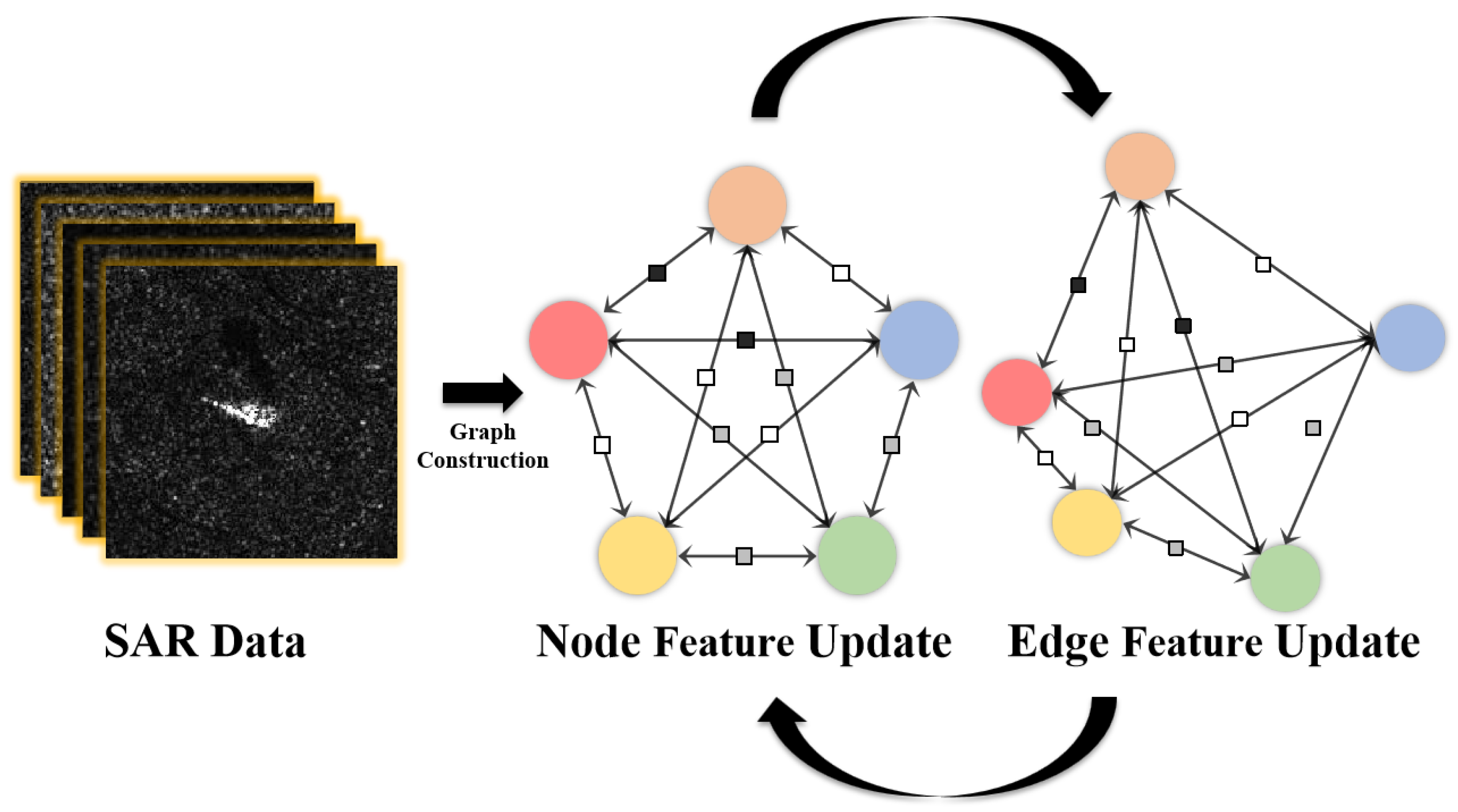
- We propose an innovative framework termed ADMM-GCN for few-shot SAR ATR, which effectively combines global context with local feature analysis by constructing a relational graph among features, thereby enhancing the overall feature representation under limited-data scenarios.
- A mixed regularized loss function is designed to mitigate the common challenge of overfitting in FSL, enhancing the model’s stability and generalizability across diverse scenarios without relying on extensive data augmentation.
- The ADMM algorithm is integrated into few-shot SAR ATR to ensure consistent convergence to the global optimum while avoiding local optima, simplifying optimization by decomposing complex problems into tractable subproblems.
- Extensive experiments conducted on the Moving and Stationary Target Acquisition and Recognition (MSTAR) dataset verify the superiority of the proposed ADMM-GCN, achieving an impressive accuracy of 92.18% on the challenging three-way 10-shot task, outperforming the benchmarks by 3.25%.
2. Related Works
2.1. Few-Shot SAR Target Recognition
2.1.1. Data-Augmentation-Based Methods
2.1.2. Model-Optimization-Based Methods
2.2. Alternating Direction Method of Multipliers
- They often converge to local optima, making it difficult to reach the global optimum and hindering the overall training process;
- Their effectiveness is highly sensitive to input data quality, requiring meticulous preprocessing to ensure convergence, which complicates training and affects model performance.
- ADMM decomposes the optimization problem into smaller, more manageable subproblems, each of which can be solved optimally with theoretical guarantees of convergence. This decomposition is particularly beneficial in FSL, where limited data necessitates a stable and structured training process.
- Unlike gradient-based methods, ADMM is inherently robust to parameter initialization, ensuring stable convergence even when training data are scarce.
- By introducing an auxiliary variable, ADMM enforces constraints during optimization, which not only stabilizes training but also enhances generalization, making it well suited for FSL applications.
3. Methodology
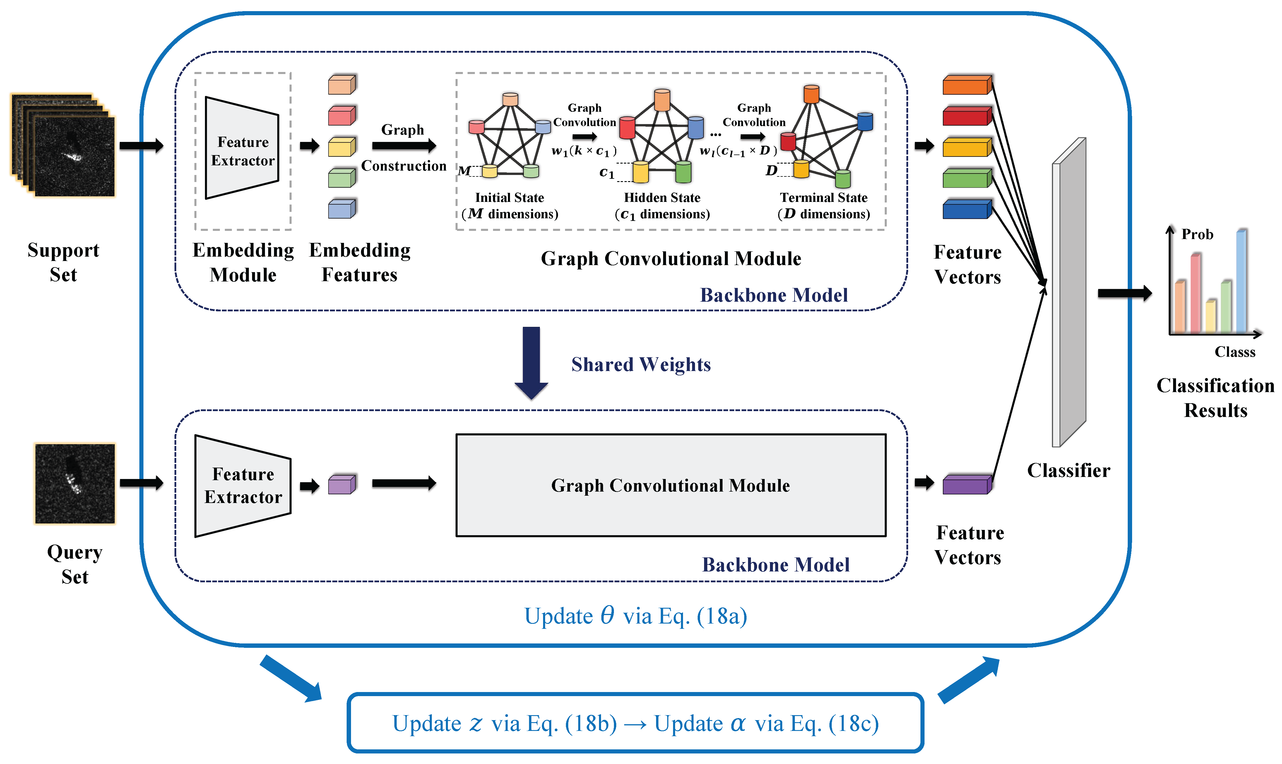
3.1. Framework of ADMM-GCN
3.2. Network Architecture
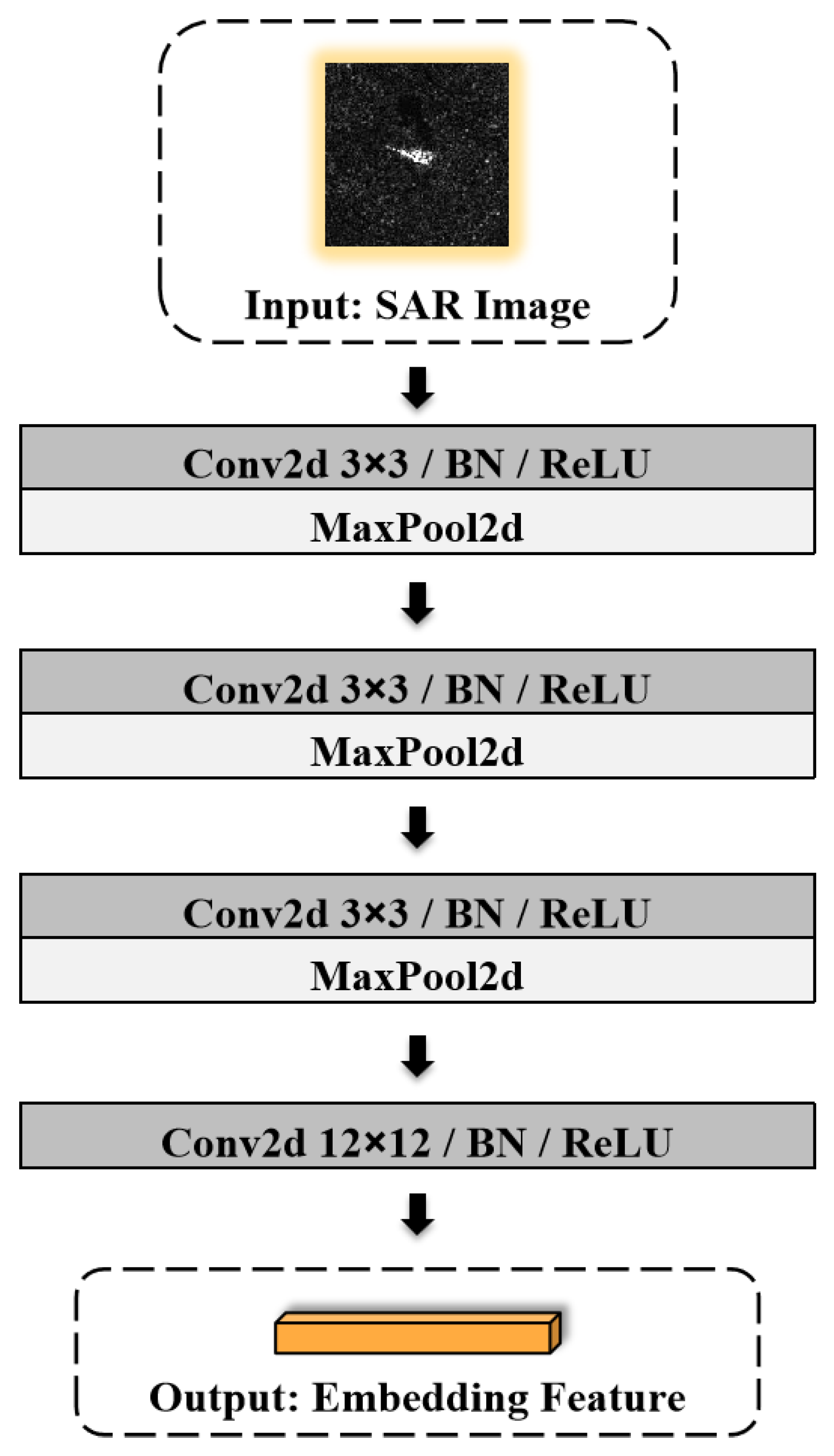
3.2.1. Embedding Module
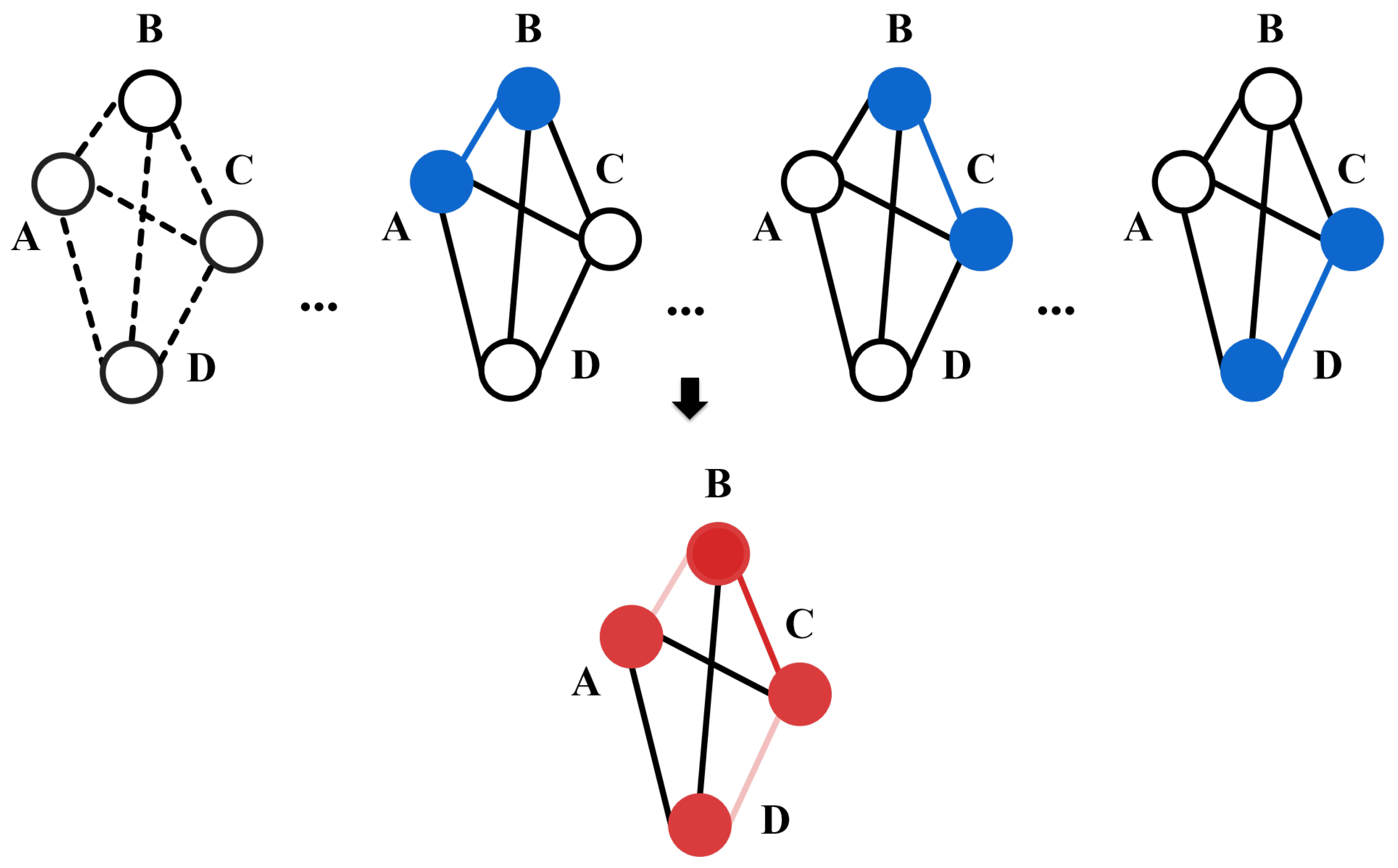
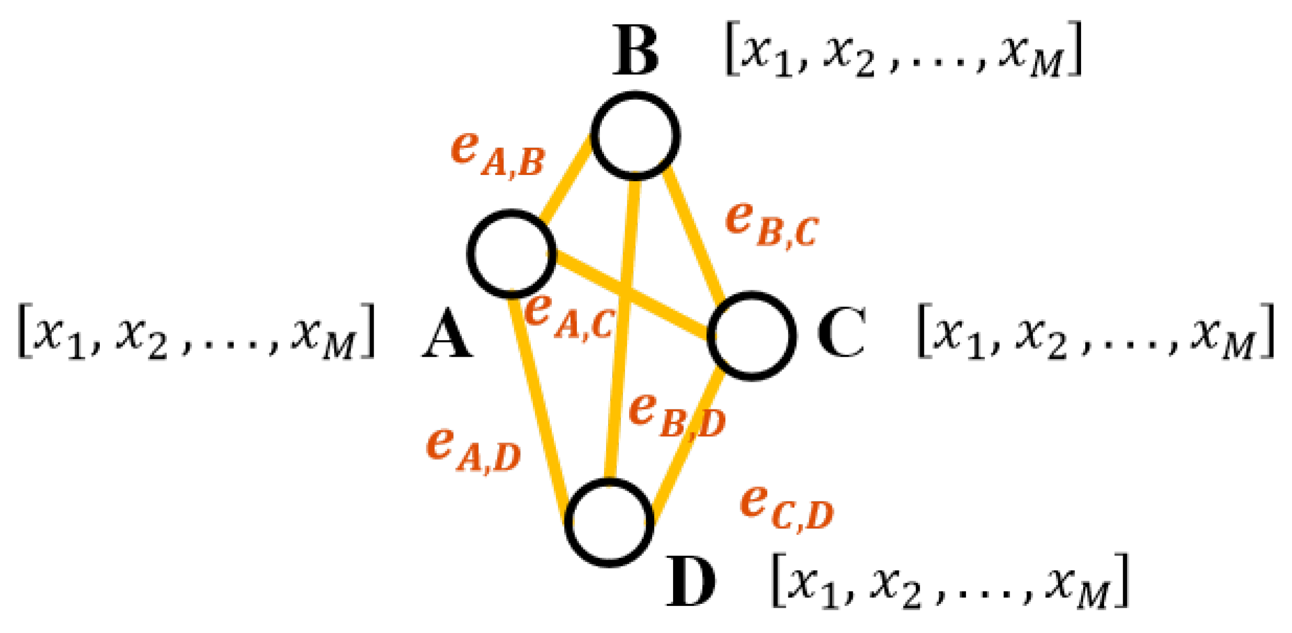
3.2.2. Graph Convolutional Module
3.3. Construction of Regularized Mixed Loss
3.4. ADMM Optimizer
| Algorithm 1 ADMM Algorithm for Optimization with Regularization |
|
4. Experiment
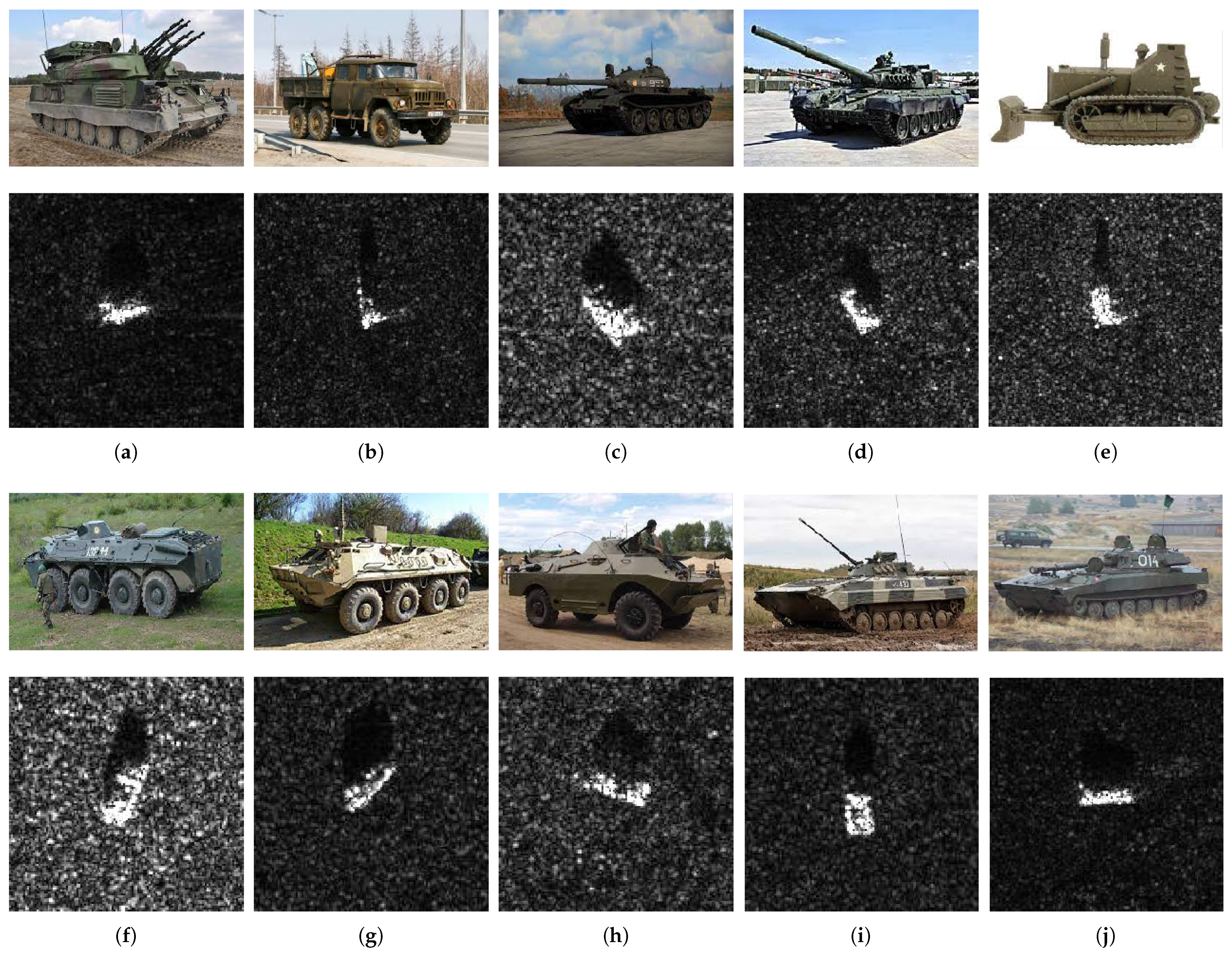
4.1. Dataset
4.2. N-Way K-Shot Task
4.3. Implementation Details
| Algorithm 2 Episode Training for ADMM-GCN |
|
5. Discussion and Analysis
5.1. Comparison Experiments
5.2. Performance Assessment Under Varying Conditions
5.3. Ablation Study
5.3.1. Effectiveness Assessment of the EM
5.3.2. Effectiveness Assessment of the GCM
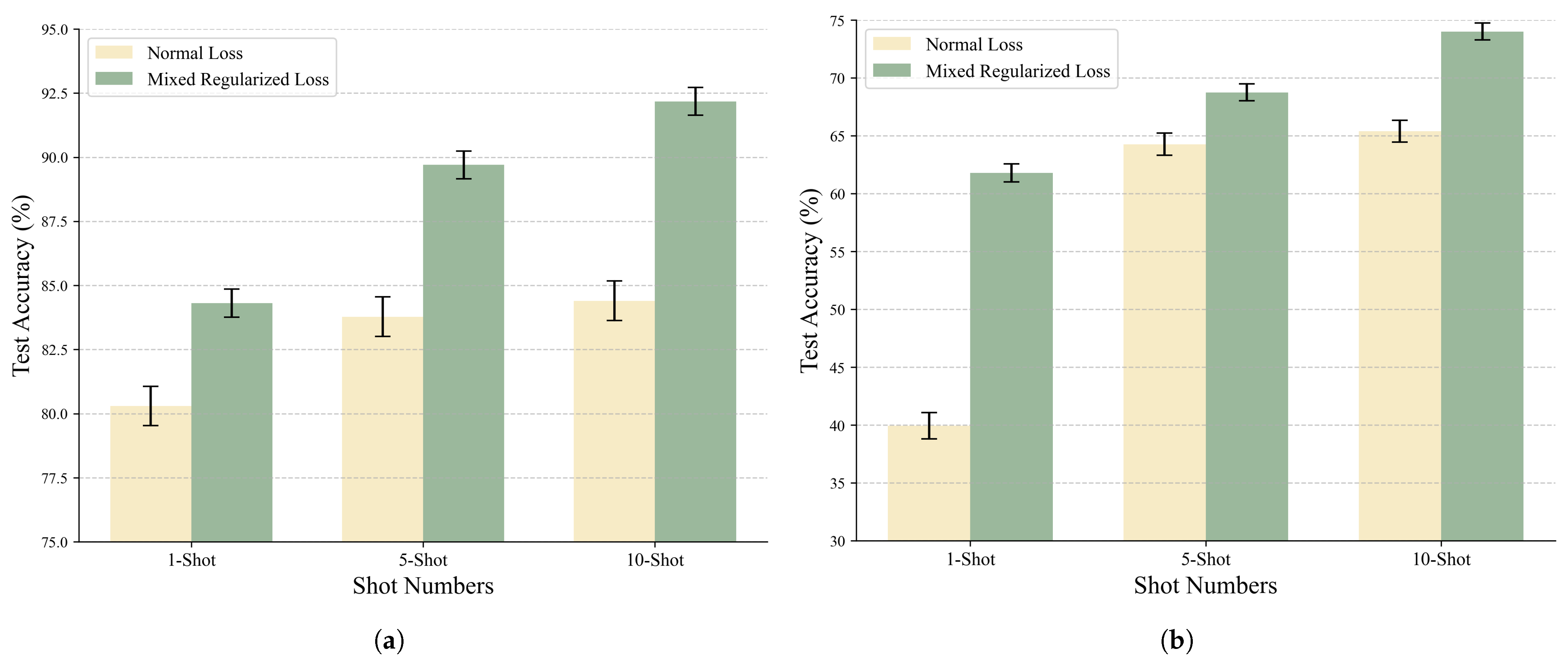
5.3.3. Impact Evaluation of Mixed Regularized Loss
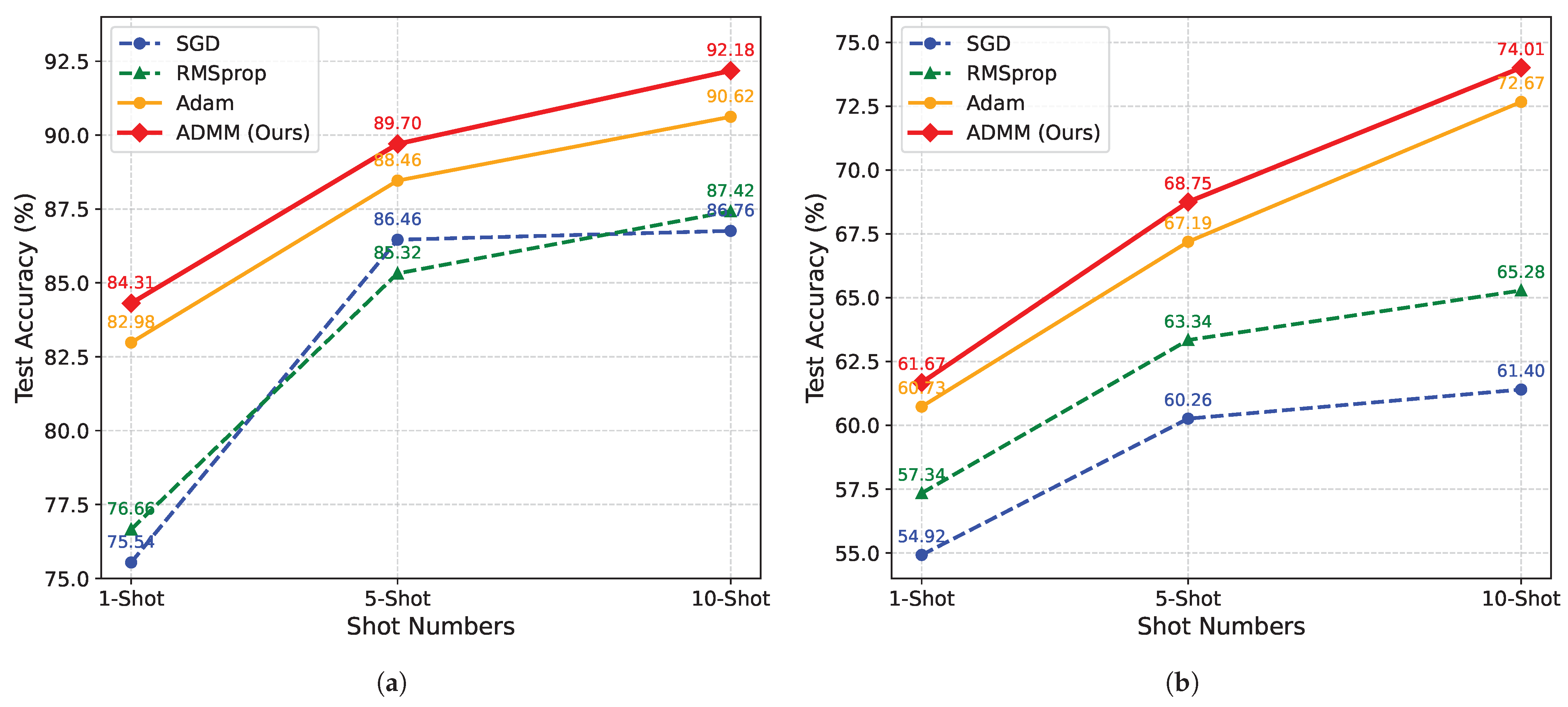
5.3.4. Performance of ADMM Optimizer
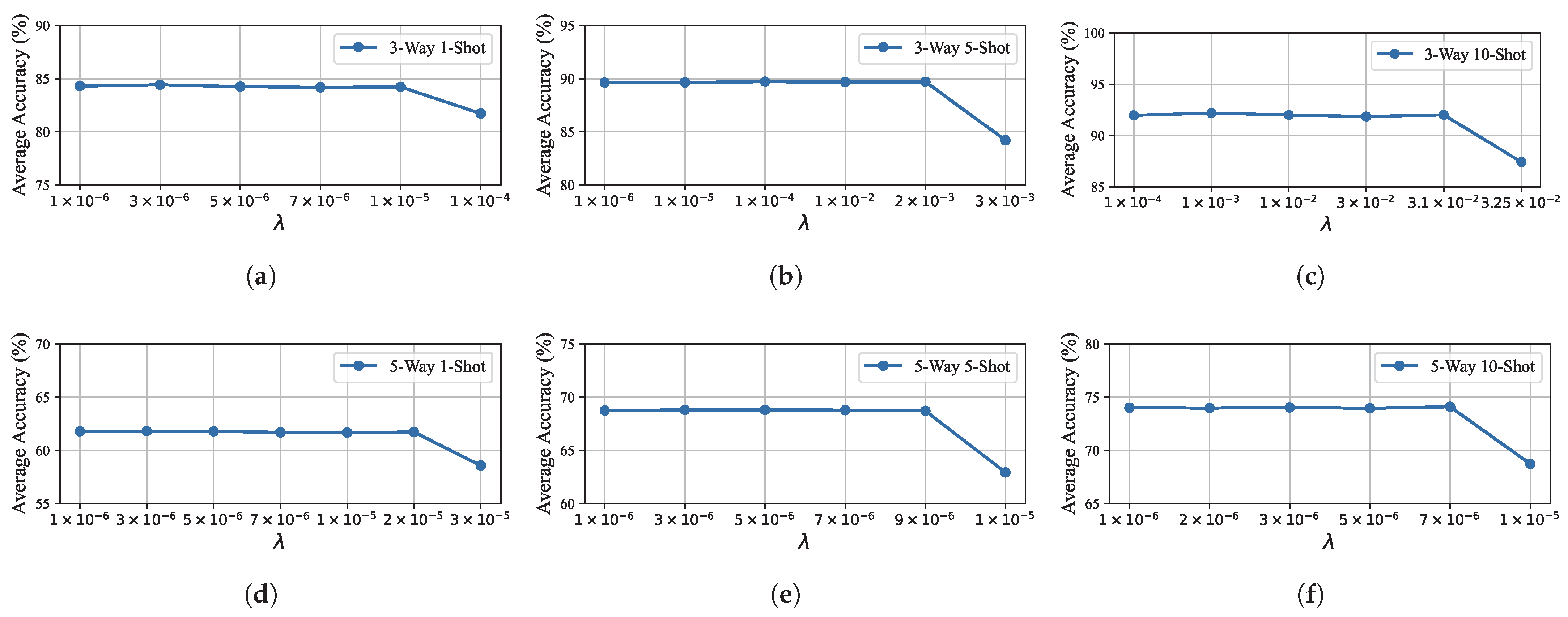
5.4. Hyperparameter Analysis
6. Conclusions
Author Contributions
Funding
Data Availability Statement
Conflicts of Interest
Abbreviations
| ADMM | Alternating Direction Method Of Multipliers |
| ATR | Automatic Target Recognition |
| CNN | Convolutional Neural Network |
| EO | Electro-Optical |
| EM | Embedding Module |
| FSL | Few-Shot Learning |
| GCM | Graph Convolutional Module |
| GCN | Graph Convolutional Network |
| MLP | Multilayer Perceptron |
| MSTAR | Moving And Stationary Target Acquisition And Recognition |
| SAR | Synthetic Aperture Radar |
| SGD | Stochastic Gradient Descent |
| SWD | Sliced Wasserstein Distance |
| TPN | Transductive Propagation Network |
| ZSL | Zero-Shot Learning |
References
- Moreira, A.; Prats-Iraola, P.; Younis, M.; Krieger, G.; Hajnsek, I.; Papathanassiou, K.P. A tutorial on synthetic aperture radar. IEEE Geosci. Remote Sens. Mag. 2013, 1, 6–43. [Google Scholar]
- Chen, S.; Wang, H.; Xu, F.; Jin, Y.Q. Target classification using the deep convolutional networks for SAR images. IEEE Trans. Geosci. Remote Sens. 2016, 54, 4806–4817. [Google Scholar]
- Zhao, Q.; Principe, J.C. Support vector machines for SAR automatic target recognition. IEEE Trans. Aerosp. Electron. Syst. 2001, 37, 643–654. [Google Scholar]
- Ding, J.; Chen, B.; Liu, H.; Huang, M. Convolutional neural network with data augmentation for SAR target recognition. IEEE Geosci. Remote Sens. Lett. 2016, 13, 364–368. [Google Scholar]
- Cho, J.H.; Park, C.G. Multiple feature aggregation using convolutional neural networks for SAR image-based automatic target recognition. IEEE Geosci. Remote Sens. Lett. 2018, 15, 1882–1886. [Google Scholar]
- Novak, L.M.; Owirka, G.J.; Brower, W.S. Performance of 10-and 20-target MSE classifiers. IEEE Trans. Aerosp. Electron. Syst. 2000, 36, 1279–1289. [Google Scholar]
- Sun, Y.; Liu, Z.; Todorovic, S.; Li, J. Adaptive boosting for SAR automatic target recognition. IEEE Trans. Aerosp. Electron. Syst. 2007, 43, 112–125. [Google Scholar]
- Dong, G.; Kuang, G.; Wang, N.; Wang, W. Classification via sparse representation of steerable wavelet frames on Grassmann manifold: Application to target recognition in SAR image. IEEE Trans. Image Process. 2017, 26, 2892–2904. [Google Scholar]
- Dong, G.; Kuang, G.; Wang, N.; Zhao, L.; Lu, J. SAR target recognition via joint sparse representation of monogenic signal. IEEE J. Sel. Top. Appl. Earth Obs. Remote Sens. 2015, 8, 3316–3328. [Google Scholar]
- Novak, L.M.; Owirka, G.J.; Brower, W.S.; Weaver, A.L. The automatic target-recognition system in SAIP. Linc. Lab. J. 1997, 10, 187–202. [Google Scholar]
- Diemunsch, J.R.; Wissinger, J. Moving and stationary target acquisition and recognition (MSTAR) model-based automatic target recognition: Search technology for a robust ATR. In Algorithms for Synthetic Aperture Radar Imagery V, Proceedings of the Aerospace/Defense Sensing and Controls 1998, Orlando, FL, USA, 13–17 April 1998; SPIE: Bellingham, WA, USA, 1998; Volume 3370, pp. 481–492. [Google Scholar]
- Zhu, X.X.; Montazeri, S.; Ali, M.; Hua, Y.; Wang, Y.; Mou, L.; Shi, Y.; Xu, F.; Bamler, R. Deep learning meets SAR: Concepts, models, pitfalls, and perspectives. IEEE Geosci. Remote Sens. Mag. 2021, 9, 143–172. [Google Scholar]
- Oveis, A.H.; Giusti, E.; Ghio, S.; Martorella, M. A survey on the applications of convolutional neural networks for synthetic aperture radar: Recent advances. IEEE Aerosp. Electron. Syst. Mag. 2021, 37, 18–42. [Google Scholar]
- Khan, M.; Saddik, A.E.; Deriche, M.; Gueaieb, W. STT-Net: Simplified Temporal Transformer for Emotion Recognition. IEEE Access 2024, 12, 86220–86231. [Google Scholar] [CrossRef]
- Khan, M.; Khan, U.; Othmani, A. PD-Net: Multi-Stream Hybrid Healthcare System for Parkinson’s Disease Detection using Multi Learning Trick Approach. In Proceedings of the 2023 IEEE 36th International Symposium on Computer-Based Medical Systems (CBMS), L’Aquila, Italy, 22–24 June 2023; pp. 382–385. [Google Scholar] [CrossRef]
- Khan, M.; Gueaieb, W.; Saddik, A.E.; De Masi, G.; Karray, F. An Efficient Violence Detection Approach for Smart Cities Surveillance System. In Proceedings of the 2023 IEEE International Smart Cities Conference (ISC2), Bucharest, Romania, 24–27 September 2023; pp. 1–5. [Google Scholar] [CrossRef]
- Bai, X.; Xue, R.; Wang, L.; Zhou, F. Sequence SAR image classification based on bidirectional convolution-recurrent network. IEEE Trans. Geosci. Remote Sens. 2019, 57, 9223–9235. [Google Scholar]
- Zhou, F.; Wang, L.; Bai, X.; Hui, Y. SAR ATR of ground vehicles based on LM-BN-CNN. IEEE Trans. Geosci. Remote Sens. 2018, 56, 7282–7293. [Google Scholar]
- Huang, Z.; Pan, Z.; Lei, B. What, where, and how to transfer in SAR target recognition based on deep CNNs. IEEE Trans. Geosci. Remote Sens. 2019, 58, 2324–2336. [Google Scholar]
- Wang, P.; Sun, X.; Diao, W.; Fu, K. FMSSD: Feature-merged single-shot detection for multiscale objects in large-scale remote sensing imagery. IEEE Trans. Geosci. Remote Sens. 2019, 58, 3377–3390. [Google Scholar]
- Sun, X.; Liu, Y.; Yan, Z.; Wang, P.; Diao, W.; Fu, K. SRAF-Net: Shape robust anchor-free network for garbage dumps in remote sensing imagery. IEEE Trans. Geosci. Remote Sens. 2020, 59, 6154–6168. [Google Scholar]
- He, Q.; Sun, X.; Yan, Z.; Fu, K. DABNet: Deformable contextual and boundary-weighted network for cloud detection in remote sensing images. IEEE Trans. Geosci. Remote Sens. 2021, 60, 5601216. [Google Scholar]
- Wang, Y.; Yao, Q.; Kwok, J.T.; Ni, L.M. Generalizing from a few examples: A survey on few-shot learning. ACM Comput. Surv. (CSUR) 2020, 53, 1–34. [Google Scholar]
- Sun, X.; Wang, B.; Wang, Z.; Li, H.; Li, H.; Fu, K. Research progress on few-shot learning for remote sensing image interpretation. IEEE J. Sel. Top. Appl. Earth Obs. Remote Sens. 2021, 14, 2387–2402. [Google Scholar] [CrossRef]
- Du, K.; Deng, Y.; Wang, R.; Zhao, T.; Li, N. SAR ATR based on displacement-and rotation-insensitive CNN. Remote Sens. Lett. 2016, 7, 895–904. [Google Scholar] [CrossRef]
- Wagner, S.A. SAR ATR by a combination of convolutional neural network and support vector machines. IEEE Trans. Aerosp. Electron. Syst. 2016, 52, 2861–2872. [Google Scholar]
- Song, Q.; Xu, F.; Zhu, X.X.; Jin, Y.Q. Learning to generate SAR images with adversarial autoencoder. IEEE Trans. Geosci. Remote Sens. 2021, 60, 5210015. [Google Scholar]
- Sun, Y.; Wang, Y.; Liu, H.; Wang, N.; Wang, J. SAR target recognition with limited training data based on angular rotation generative network. IEEE Geosci. Remote Sens. Lett. 2019, 17, 1928–1932. [Google Scholar]
- Rostami, M.; Kolouri, S.; Eaton, E.; Kim, K. Deep transfer learning for few-shot SAR image classification. Remote Sens. 2019, 11, 1374. [Google Scholar] [CrossRef]
- Tai, Y.; Tan, Y.; Xiong, S.; Sun, Z.; Tian, J. Few-shot transfer learning for sar image classification without extra sar samples. IEEE J. Sel. Top. Appl. Earth Obs. Remote Sens. 2022, 15, 2240–2253. [Google Scholar]
- Wang, S.; Wang, Y.; Liu, H.; Sun, Y. Attribute-guided multi-scale prototypical network for few-shot SAR target classification. IEEE J. Sel. Top. Appl. Earth Obs. Remote Sens. 2021, 14, 12224–12245. [Google Scholar]
- Ren, H.; Liu, S.; Yu, X.; Zou, L.; Zhou, Y.; Wang, X.; Tang, H. Transductive Prototypical Attention Reasoning Network for Few-shot SAR Target Recognition. IEEE Trans. Geosci. Remote. Sens. 2023, 61, 5206813. [Google Scholar] [CrossRef]
- Fu, K.; Zhang, T.; Zhang, Y.; Wang, Z.; Sun, X. Few-shot SAR target classification via metalearning. IEEE Trans. Geosci. Remote Sens. 2021, 60, 2000314. [Google Scholar] [CrossRef]
- Kingma, D.P.; Ba, J. Adam: A method for stochastic optimization. arXiv 2014, arXiv:1412.6980. [Google Scholar]
- Robbins, H.; Monro, S. A Stochastic Approximation Method. Ann. Math. Stat. 1951, 22, 400–407. [Google Scholar]
- Boyd, S.; Parikh, N.; Chu, E.; Peleato, B.; Eckstein, J. Distributed optimization and statistical learning via the alternating direction method of multipliers. Found. Trends® Mach. Learn. 2011, 3, 1–122. [Google Scholar]
- Wang, J.; Yu, F.; Chen, X.; Zhao, L. ADMM for Efficient Deep Learning with Global Convergence. In Proceedings of the 25th ACM SIGKDD International Conference on Knowledge Discovery & Data Mining, Anchorage AK, USA, 4–8 August 2019; ACM: New York, NY, USA, 2019. [Google Scholar] [CrossRef]
- Yang, Y.; Sun, J.; Li, H.; Xu, Z. ADMM-CSNet: A Deep Learning Approach for Image Compressive Sensing. IEEE Trans. Pattern Anal. Mach. Intell. 2020, 42, 521–538. [Google Scholar] [CrossRef] [PubMed]
- Lin, C.H.; Lin, Y.C.; Tang, P.W. ADMM-ADAM: A New Inverse Imaging Framework Blending the Advantages of Convex Optimization and Deep Learning. IEEE Trans. Geosci. Remote Sens. 2022, 60, 5514616. [Google Scholar] [CrossRef]
- Kipf, T.N.; Welling, M. Semi-supervised classification with graph convolutional networks. arXiv 2016, arXiv:1609.02907. [Google Scholar]
- Zhang, Z.; Cui, P.; Zhu, W. Deep learning on graphs: A survey. IEEE Trans. Knowl. Data Eng. 2020, 34, 249–270. [Google Scholar]
- Hong, M.; Luo, Z.Q.; Razaviyayn, M. Convergence analysis of alternating direction method of multipliers for a family of nonconvex problems. SIAM J. Optim. 2016, 26, 337–364. [Google Scholar] [CrossRef]
- Wang, Y.; Yin, W.; Zeng, J. Global convergence of ADMM in nonconvex nonsmooth optimization. J. Sci. Comput. 2019, 78, 29–63. [Google Scholar]
- Cascarano, P.; Calatroni, L.; Piccolomini, E.L. On the inverse Potts functional for single-image super-resolution problems. arXiv 2020, arXiv:2008.08470. [Google Scholar]
- Maclaurin, D.; Duvenaud, D.; Adams, R.P. Autograd: Effortless gradients in numpy. In Proceedings of the ICML 2015 AutoML Workshop, Lille, France, 11 July 2015; Volume 238. [Google Scholar]
- Xu, Z.; Luo, Y.; Wu, B.; Meng, D. S2S-WTV: Seismic Data Noise Attenuation Using Weighted Total Variation Regularized Self-Supervised Learning. IEEE Trans. Geosci. Remote. Sens. 2023, 61, 5908315. [Google Scholar]
- Defense Advanced Research Project Agency (DARPA); Air Force Research Laboratory (AFRL). The Air Force Moving and Stationary Target Recognition (MSTAR) Database. 2014. Available online: https://www.sdms.afrl.af.mil/index.php?collection=mstar (accessed on 1 January 2024).
- Koch, G.; Zemel, R.; Salakhutdinov, R. Siamese neural networks for one-shot image recognition. In Proceedings of the ICML Deep Learning Workshop, Lille, France, 6–11 July 2015; Volume 2. [Google Scholar]
- Vinyals, O.; Blundell, C.; Lillicrap, T.; Wierstra, D. Matching networks for one shot learning. In Proceedings of the Advances in Neural Information Processing Systems 29: Annual Conference on Neural Information Processing Systems 2016, Barcelona, Spain, 5–10 December 2016; Volume 29. [Google Scholar]
- Snell, J.; Swersky, K.; Zemel, R. Prototypical networks for few-shot learning. In Proceedings of the Advances in Neural Information Processing Systems 30: Annual Conference on Neural Information Processing Systems 2017, Long Beach, CA, USA, 4–9 December 2017; Volume 30. [Google Scholar]
- Sung, F.; Yang, Y.; Zhang, L.; Xiang, T.; Torr, P.H.; Hospedales, T.M. Learning to compare: Relation network for few-shot learning. In Proceedings of the IEEE Conference on Computer Vision and Pattern Recognition, Salt Lake City, UT, USA, 18–23 June 2018; pp. 1199–1208. [Google Scholar]
- Liu, Y.; Lee, J.; Park, M.; Kim, S.; Yang, E.; Hwang, S.J.; Yang, Y. Learning to propagate labels: Transductive propagation network for few-shot learning. arXiv 2018, arXiv:1805.10002. [Google Scholar]
- Zhang, C.; Cai, Y.; Lin, G.; Shen, C. DeepEMD: Few-shot image classification with differentiable earth mover’s distance and structured classifiers. In Proceedings of the IEEE/CVF Conference on Computer Vision and Pattern Recognition, Seattle, WA, USA, 13–19 June 2020; pp. 12203–12213. [Google Scholar]
- Liu, S.; Yu, X.; Ren, H.; Zou, L.; Zhou, Y.; Wang, X. Bi-similarity prototypical network with capsule-based embedding for few-shot sar target recognition. In Proceedings of the IGARSS 2022—2022 IEEE International Geoscience and Remote Sensing Symposium, Kuala Lumpur, Malaysia, 17–22 July 2022; IEEE: New York, NY, USA, 2022; pp. 1015–1018. [Google Scholar]
- Tibshirani, R. Regression shrinkage and selection via the lasso. J. R. Stat. Soc. Ser. B Stat. Methodol. 1996, 58, 267–288. [Google Scholar]
- Zou, H.; Hastie, T. Regularization and variable selection via the elastic net. J. R. Stat. Soc. Ser. B Stat. Methodol. 2005, 67, 301–320. [Google Scholar]
- Hinton, G.; Srivastava, N.; Swersky, K. Neural networks for machine learning lecture 6a overview of mini-batch gradient descent. Cited 2012, 14, 2. [Google Scholar]


| Target Category | BRDM2 | BMP2 | BTR60 | BTR70 | D7 | T62 | T72 | ZIL131 | ZSU234 | 2S1 |
| Number | 572 | 428 | 451 | 429 | 573 | 572 | 428 | 573 | 573 | 573 |
| N-Way K-Shot Task | Categories | Categories |
|---|---|---|
| 5-way K-shot | ZIL131, BMP2, T62, BTR70, ZSU234 | BTR60, BRDM2, T72, 2S1, D7 |
| 3-way K-shot | D7, T62, 2S1, ZIL131, BMP2, ZSU234, BTR70 | BTR60, BRDM2, T72 |
| Methods | 3-Way | 5-Way | ||||
|---|---|---|---|---|---|---|
| 1-Shot | 5-Shot | 10-Shot | 1-Shot | 5-Shot | 10-Shot | |
| ProtoNet [50] | 71.24 ± 0.45 | 80.79 ± 0.38 | 82.37 ± 0.33 | 50.42 ± 0.89 | 63.74 ± 0.78 | 67.95 ± 0.70 |
| RelationNet [51] | 75.32 ± 0.49 | 84.29 ± 0.43 | 86.76 ± 0.35 | 53.81 ± 0.91 | 66.52 ± 0.84 | 72.20 ± 0.62 |
| TPN [52] | 80.45 ± 0.48 | 87.32 ± 0.46 | 88.93 ± 0.42 | 57.44 ± 0.92 | 65.70 ± 0.83 | 70.37 ± 0.73 |
| MSAR [33] | 69.23 ± 0.51 | 84.71 ± 0.59 | 87.96 ± 0.49 | 53.50 ± 1.00 | 60.50 ± 0.90 | 64.72 ± 0.71 |
| DeepEMD [53] | 76.01 ± 0.42 | 83.23 ± 0.39 | 86.24 ± 0.34 | 55.61 ± 0.82 | 65.17 ± 0.75 | 69.66 ± 0.60 |
| BSCapNet [54] | 73.01 ± 0.47 | 86.62 ± 0.48 | 84.60 ± 0.42 | 64.81 ± 0.87 | 67.50 ± 0.79 | 73.55 ± 0.56 |
| ADMM-GCN (ours) | 84.31 ± 0.39 | 89.70 ± 0.39 | 92.18 ± 0.38 | 61.79 ± 0.56 | 68.75 ± 0.52 | 74.01 ± 0.53 |
| Perturbation Settings | 3-Way | 5-Way | ||||||
|---|---|---|---|---|---|---|---|---|
| Noise Injection | Random Cropping | Rotation | 1-Shot | 5-Shot | 10-Shot | 1-Shot | 5-Shot | 10-Shot |
| 84.31 | 89.70 | 92.18 | 61.79 | 68.75 | 74.01 | |||
| ✓ | 81.38 | 89.62 | 90.26 | 60.12 | 66.04 | 73.74 | ||
| ✓ | 80.32 | 88.70 | 90.02 | 61.46 | 64.62 | 73.80 | ||
| ✓ | 82.32 | 89.06 | 90.50 | 58.44 | 65.82 | 72.16 | ||
| ✓ | ✓ | ✓ | 81.10 | 89.58 | 90.88 | 56.98 | 65.46 | 71.10 |
| N-Way | EM Settings | K-Shot | ||
|---|---|---|---|---|
| 1-Shot | 5-Shot | 10-Shot | ||
| 3-way | w/o EM | 72.61 | 75.43 | 78.25 |
| w EM | 84.31 (11.70 ↑) | 89.70 (14.27 ↑) | 92.18 (13.93 ↑) | |
| 5-way | w/o EM | 58.48 | 68.69 | 72.34 |
| w EM | 61.79 (3.31 ↑) | 68.75 (0.06↑) | 74.01 (1.67 ↑) | |
| N-Way | GCM Settings | K-Shot | ||
|---|---|---|---|---|
| 1-Shot | 5-Shot | 10-Shot | ||
| 3-way | w/o GCM | 70.63 | 87.99 | 90.16 |
| w GCM | 84.31 (13.68 ↑) | 89.70 (1.71 ↑) | 92.18 (2.02 ↑) | |
| 5-way | w/o GCM | 56.85 | 65.68 | 72.70 |
| w GCM | 61.79 (4.94 ↑) | 68.75 (3.07 ↑) | 74.01 (1.31 ↑) | |
| Configurations | Accuracy (%) | |||||
|---|---|---|---|---|---|---|
| Loss Settings | -Shot | Min | Max | Mean | Standard Deviation | |
| Classical Loss | 1-shot | 78.64 | 82.57 | 80.30 | 0.7684 | |
| 5-shot | 81.46 | 85.26 | 83.78 | 0.7745 | ||
| 10-shot | 82.00 | 86.79 | 84.40 | 0.7697 | ||
| Mixed Regularized Loss | 1-shot | 82.67 | 86.79 | 84.31 (4.01 ↑) | 0.5467 (0.2217 ↓) | |
| 5-shot | 88.50 | 90.86 | 89.70 (5.92 ↑) | 0.5440 (0.2305 ↓) | ||
| 10-shot | 90.50 | 93.43 | 92.18 (7.78 ↑) | 0.5374 (0.2323 ↓) | ||
| Configurations | Accuracy (%) | |||||
|---|---|---|---|---|---|---|
| Loss Settings | -Shot | Min | Max | Mean | Standard Deviation | |
| Classical Loss | 1-shot | 37.14 | 43.07 | 39.94 | 1.1498 | |
| 5-shot | 62.07 | 66.50 | 64.27 | 0.9465 | ||
| 10-shot | 64.56 | 65.82 | 65.40 | 0.9453 | ||
| Mixed Regularized Loss | 1-shot | 59.14 | 65.21 | 61.79 (21.85 ↑) | 0.7856 (0.3642 ↓) | |
| 5-shot | 65.21 | 69.57 | 68.75 (4.48 ↑) | 0.7198 (0.2267 ↓) | ||
| 10-shot | 71.43 | 76.29 | 74.01 (8.61 ↑) | 0.7384 (0.2069 ↓) | ||
| Regularization Settings | 3-Way | 5-Way | ||||
|---|---|---|---|---|---|---|
| 1-Shot | 5-Shot | 10-Shot | 1-Shot | 5-Shot | 10-Shot | |
| L1 Regularization [55] | 67.06 | 85.48 | 85.84 | 57.96 | 63.18 | 67.64 |
| ElasticNet [56] | 80.84 | 87.28 | 91.44 | 58.04 | 67.40 | 66.12 |
| Mixed Regularized Loss | 84.31 | 89.70 | 92.18 | 61.79 | 68.75 | 74.01 |
Disclaimer/Publisher’s Note: The statements, opinions and data contained in all publications are solely those of the individual author(s) and contributor(s) and not of MDPI and/or the editor(s). MDPI and/or the editor(s) disclaim responsibility for any injury to people or property resulting from any ideas, methods, instructions or products referred to in the content. |
© 2025 by the authors. Licensee MDPI, Basel, Switzerland. This article is an open access article distributed under the terms and conditions of the Creative Commons Attribution (CC BY) license (https://creativecommons.org/licenses/by/4.0/).
Share and Cite
Jin, J.; Xu, Z.; Zheng, N.; Wang, F. Graph-Based Few-Shot Learning for Synthetic Aperture Radar Automatic Target Recognition with Alternating Direction Method of Multipliers. Remote Sens. 2025, 17, 1179. https://doi.org/10.3390/rs17071179
Jin J, Xu Z, Zheng N, Wang F. Graph-Based Few-Shot Learning for Synthetic Aperture Radar Automatic Target Recognition with Alternating Direction Method of Multipliers. Remote Sensing. 2025; 17(7):1179. https://doi.org/10.3390/rs17071179
Chicago/Turabian StyleJin, Jing, Zitai Xu, Nairong Zheng, and Feng Wang. 2025. "Graph-Based Few-Shot Learning for Synthetic Aperture Radar Automatic Target Recognition with Alternating Direction Method of Multipliers" Remote Sensing 17, no. 7: 1179. https://doi.org/10.3390/rs17071179
APA StyleJin, J., Xu, Z., Zheng, N., & Wang, F. (2025). Graph-Based Few-Shot Learning for Synthetic Aperture Radar Automatic Target Recognition with Alternating Direction Method of Multipliers. Remote Sensing, 17(7), 1179. https://doi.org/10.3390/rs17071179