A Target Near-Field Scattering Measurement Technique Utilizing 3D Near-Field Imaging via Cylindrical Scanning

Abstract

Radar target near-field scattering characteristics are essential for the identification of target properties and the improvement of target recognition. Nevertheless, the efficiency of current precision three-dimensional (3D) imaging algorithms in near-field scattering measurements is restricted by their substantial computational complexity. To resolve this matter, we propose a hybrid 3D imaging algorithm that is optimized for cylindrical sampling and operates in both the wavenumber domain and time domain (WDTD). Wavenumber domain algorithms are initially utilized for the rapid localization of strong scattering sources. Subsequently, morphological image analysis techniques are employed to delineate the regions containing strong scattering sources. Ultimately, accurate calculations are performed utilizing backpropagation (BP) in time domain algorithms. This method significantly reduces the computational burden while maintaining imaging accuracy by integrating rapid scattering source extraction with precise computation for critical regions. The proposed capacity to accomplish efficient and precise 3D imaging is effectively demonstrated by the experimental results, which effectively mitigate the computational challenges associated with traditional algorithms. Furthermore, the method effectively reconstructs near-field echoes of scattering sources, underscoring its potential for decoupling target–background interactions. The versatility of this method is further demonstrated by its ability to be applied to other 3D imaging configurations, which illustrates its potential to advance radar imaging technologies and near-field scattering research.

1. Introduction

The near-field scattering characteristics of radar targets reflect the intrinsic physical properties of the target, including the shape, size, and structure, as well as antenna parameters such as the polarization, frequency, waveform, and orientation angles, within specific electromagnetic environments. Examining near-field scattering characteristics enhances our comprehension of the interaction mechanisms between electromagnetic waves and objects, and is essential for target recognition [1] and stealth design [2]. This research possesses considerable scientific value. Radar imaging measurement methods are a significant aspect of this field [3], representing both a key direction for technological advancement and a prominent area of current research interest.

The measurement of radar target near-field scattering characteristics is often complicated by the electromagnetic environment [4], including background noise, ground clutters, and multipath effects, which can introduce significant interference and hinder the measurement accuracy. Traditional measurement methods have limitations in flexibly analyzing the overall or local scattering distribution of the target and are ineffective in quickly diagnosing scattering defects, thereby constraining the information obtainable in radar target studies. Research on scattering characteristics related to radar target imaging provides an effective solution to address these issues [5]. This method’s fundamental principle is the use of a synthetic aperture antenna or a virtual synthetic aperture generated by target rotation to emit broadband frequency-sweeping signals for close-range scanning of the target area, while concurrently receiving the scattered echo data. High-resolution radar imaging algorithms are subsequently applied to process the echo data, resulting in the spatial scattering distribution of the target. This approach integrates techniques including environmental removal [6], radiation correction [7], near-to-far-field compensation [8], and the measurement of both overall and local scattering characteristics of the target [9]. Radar imaging measurement presents notable advantages over traditional methods, such as enhanced resolution, diagnostic capabilities for both overall and local scattering characteristics, and the efficient suppression of environmental interference. Additionally, 3D radar imaging methods have shown significant effectiveness in overcoming challenges like multipath effects [10], attracting growing interest from researchers. In 2020, the IEEE Antennas and Propagation Society officially recommended the radar imaging measurement method as a standard testing approach for electromagnetic scattering [11], emphasizing its significant application prospects and market potential.

Numerous imaging algorithms have been developed for 3D microwave imaging, such as the 3D Range-Doppler (RD) algorithm [12], the 3D Chirp Scaling (CS) algorithm [13], the wavenumber domain (ω-k) algorithm [14], and the 3D Back-Projection (BP) algorithm [15]. The RD, CS, and ω-k algorithms incorporate approximations in the imaging process, leading to an inherent degree of error. The BP algorithm, which circumvents such approximations, is regarded as the most widely utilized and effective 3D microwave imaging algorithm available today. Nonetheless, the 3D BP algorithm presents a notable limitation: its imaging process necessitates a point-by-point scan of the complete imaging space, resulting in a substantial computational burden. The significant computational complexity adversely affects the efficiency of imaging using the BP algorithm for measuring radar target near-field scattering characteristics, creating a critical bottleneck that restricts its practical applications.

The study of reconstructing target scattering echoes based on radar imaging technology originated in the 1990s. J Jain et al. [16] developed a ground-to-air radar that creates ISAR images for a controlled flying aircraft, identifying dominating scattering sources and helping target diagnostics. After integrating ground-based and aerial radar systems, dynamic scattering measurement and electromagnetic discontinuity detection in operational circumstances became possible [17]. Advanced imaging approaches built on basic concepts. New near-field imaging methods improve the spatial resolution and measurement accuracy. Broquetas et al. [18] developed an ISAR technique that uses spherical-wave near-field illumination to reduce plane-wave facility costs and maintain image accuracy. A linear array scanning method for 3D near-field imaging by Liao et al. [8] used an upgraded BP algorithm to reconstruct spatially resolved scattering coefficient distributions. These advances enabled robust near-field imaging solutions. Hu et al. [9] implemented microwave imaging with spectrum modifications to measure weak scattering sources on airplanes, greatly increasing scattering measurements. These advances enabled precise and complete near-field imaging solutions. Next, specialized imaging systems for specific applications were developed. Sheen et al. [19] created a 3D millimeter-wave imaging system for hidden object detection that can scan quickly and accurately. The Pacific Northwest National Laboratory [20] developed a near-field 3D imaging system using planar scanning arrays and swept-frequency operation to assess L-X target scattering properties at a high resolution. Using a 3D radar imaging system, Minvielle et al. [21] created exact scatterer maps from X-band datasets, exceeding standard approaches in the performance and resolution. Alvarez [10] created a near-field two-dimensional lateral scanning system with excellent spatial consistency and image precision for full-scale targets in controlled conditions. Wang et al. [22] combined SIFT, APES, and CFAR algorithms with polarimetric and tomographic methods to create a full-polarimetric 3D imaging method. This method offers accurate amplitude-phase reconstruction and polarimetric decomposition, improving scattering mechanism analysis resolution and precision over standard imaging methods.

Research on extracting target near-field scattering characteristics from cylindrical sampling for 3D imaging is still relatively scarce. The near-field scattering characteristics of radar targets are essential for comprehending the intrinsic physical properties of targets and enhancing radar target recognition. The computational complexity of current 3D imaging algorithms restricts their efficacy in real-time applications. The advancement of efficient radar imaging techniques presents a significant challenge, especially in addressing the computational limitations associated with accurate 3D imaging algorithms. This study examines 3D imaging and target near-field echo reconstruction algorithms utilizing cylindrical sampling to tackle the efficiency challenges of the BP imaging algorithm. A hybrid algorithm is proposed that integrates a novel wavenumber domain approach with a fast and precise 3D imaging algorithm. This method seeks to separate target–background interactions and reconstruct near-field echoes from partial target scattering sources in near-field scattering measurements. This study’s primary contributions are summarized below:

• Fast and Precise 3D Imaging Algorithm: In the process of the 3D imaging of targets, there are significant areas devoid of scattering sources. These areas are of minimal relevance to the analysis, but they require considerable processing resources. Our suggested solution rectifies this inherent inefficiency by focused computing allocation, significantly diminishing processing overhead while maintaining imaging fidelity. This paper presents a fast and precise 3D imaging algorithm that integrates wavenumber domain and time domain (WDTD) techniques to mitigate the computational complexity and low efficiency of the existing precise 3D BP imaging algorithm. The method initially utilizes a wavenumber domain algorithm to efficiently extract the scattering source distribution of the target. Morphological operations in digital image processing are applied to identify regions that necessitate precise computation. The identified regions serve as the input to the BP algorithm, thereby completing precise imaging. WDTD effectively identifies scattering sources in the wavenumber domain and enhances imaging in key areas through time domain methods, resulting in a significant decrease in the computational complexity while maintaining accuracy.
• Potential for Decoupling Target–Background Scattering in Near-Field Measurements: This study reconstructs echoes from scattering sources that share identical mechanisms, but exhibit varying scattering intensities, as well as from sources with differing scattering mechanisms. The findings preliminarily demonstrate the method’s potential to decouple target–background scattering and selectively extract and reconstruct echoes from specific regions of interest. The proposed approach is adaptable to various 3D imaging systems that utilize different sampling geometries, including planar or spherical sampling, demonstrating its versatility and broader applicability.

The subsequent sections of this paper are structured as follows. Section 2 presents the adopted system and signal model, detailing the principles of conventional wavenumber domain and time domain imaging algorithms. The proposal includes a hybrid algorithm for fast 3D imaging that operates in both the wavenumber domain and the time domain. Section 3 outlines the configuration of the experiment system, offering a detailed description of the experimental setup and the methodologies employed for data collection. Section 4 presents and analyzes the experimental results. Section 5 details the imaging performance and efficiency improvements attained by the proposed algorithm, along with the accuracy of scattering source echo reconstruction. Section 6 provides a conclusion to this study.

2. Methods

2.1. System Model

Figure 1 illustrates the model of the cylindrical scanning 3D imaging system. The imaging Cartesian coordinate system is defined with its origin at the center of the turntable. The coordinates of any imaging position are denoted by $P_n\left(x_n,y_n,z_n\right)$ and the corresponding scattering intensity is $\sigma \left(x_n,y_n,z_n\right)$. The distance from the cylindrical sampling array of length $L_Z$ to the z-axis of the imaging coordinate system is $R$. During the rotation of the turntable, the antenna array effectively rotates around the target under measurement along a circular path with a radius $R$, thereby forming a virtual circular synthetic aperture. The coordinates of the radar transmit–receive positions are $\left(R\cos \theta ,R\sin \theta ,{\mathrm{z}}^{\prime }\right)$.

The transmitted radar signal is defined as $p\left(t\right)$. The effects of antenna directivity and propagation distance attenuation can be eliminated through standard calibration. By neglecting these two factors, the echo signal received by the radar at point $P_n$ is expressed as

$$S_n\left(t,\theta ,z^{\prime }\right)=\sigma \left(x_n,y_n,z_n\right)p\left(t-{\displaystyle \frac{2d_n}{c}}\right)$$

(1)

where $d_n=\sqrt{{\left(x_n-R\cos \theta \right)}^2+{\left(y_n-R\sin \theta \right)}^2+{\left(z_n-{\mathrm{z}}^{\prime }\right)}^2}$, and $\sigma$ represents the spatial reflectivity of the target, corresponding to the target’s image. By performing a Fourier transform of the above equation along the $t$ direction, we obtain

$$S_n\left(\omega ,\theta ,z^{\prime }\right)=P\left(\omega \right)\sigma \left(x_n,y_n,z_n\right){\mathrm{e}}^{-j2k{d}_n}$$

(2)

where $k=\omega /c$ represents the wavenumber. In practical scenarios, the echo signal of the target reflects the cumulative sum of echo signals from multiple point targets within the imaging region. Thus, the previous equation can be expressed as:

$$S\left(\omega ,\theta ,z^{\prime }\right)=P\left(\omega \right){\displaystyle \iiint \sigma \left(x,y,z\right){\mathrm{e}}^{-j2k\sqrt{{\left(x-R\cos \theta \right)}^2+{\left(y-R\sin \theta \right)}^2+{\left(z-{\mathrm{z}}^{\prime }\right)}^2}}\mathrm{d}x\mathrm{d}y\mathrm{d}z}$$

(3)

2.2. Traditional Wavenumber Domain Algorithm

The dispersion relation of the plane wave component is given by

$$k_x^2+k_y^2+k_{z^{\prime }}^2={\left(2k\right)}^2$$

(4)

where $k_x$, $k_y$, and $k_{z\prime }$ represent the wavenumber components of the spherical wave in the spatial wavenumber domain along the Cartesian coordinate system’s axes. Defining the cylindrical coordinate system wavenumber $k_r$, we have

$$\left\{\begin{array}{l}{k}_r=\sqrt{k_x^2+k_y^2}=\sqrt{4k^2-k_{z^{\prime }}^2}\\ k_x=k_r\cos \phi \\ k_y=k_r\sin \phi \end{array}\right.$$

(5)

By performing a plane wave spectral decomposition on the phase term in the echo signal, we obtain

$$\begin{array}{l}{ \mathrm{e}}^{-\mathrm{j}2k\sqrt{{(x-R\cos \theta )}^2+{(y-R\sin \theta )}^2+{\left(z-z^{\prime }\right)}^2}}\\ ={\displaystyle \iint {\mathrm{e}}^{-\mathrm{j}\left(k_r\cos \phi (x-R\cos \theta )+k_r\sin \phi (y-R\sin \theta )+k_{z^{\prime }}\left(z-z^{\prime }\right)\right)}\mathrm{d}\phi \mathrm{d}{k}_{z^{\prime }}}\\ ={\displaystyle \iint {\mathrm{e}}^{-\mathrm{j}\left(k_r\cos \phi \cdot x+k_r\sin \phi \cdot y+k_{z^{\prime }}(z-z^{\prime })-k_{r}R(\cos \phi \cos \theta +\sin \phi \sin \theta )\right)}\mathrm{d}\phi \mathrm{d}{k}_{z^{\prime }}}\\ ={\displaystyle \iint {\mathrm{e}}^{-\mathrm{j}\left(k_r\cos \phi \cdot x+k_r\sin \phi \cdot y+k_{z^{\prime }}(z-z^{\prime })-k_{r}R\cos (\phi -\theta )\right)}\mathrm{d}\phi \mathrm{d}{k}_{z^{\prime }}}\end{array}$$

(6)

Substituting Equation (6) into Equation (3) and rearranging the order of integration yields

$$S(\omega ,\theta ,z^{\prime })=P\left(\omega \right){\displaystyle \iint {\mathrm{e}}^{\mathrm{j}{k}_{r}R\cos (\phi -\theta )}\cdot }[{\displaystyle \iiint \sigma (x,y,z){\mathrm{e}}^{-\mathrm{j}(k_r\cos \phi \cdot x+k_r\sin \phi \cdot y+k_{z^{\prime }}z)}\mathrm{d}x\mathrm{d}y\mathrm{d}z}]\cdot {\mathrm{e}}^{\mathrm{j}{k}_z{z}^{\prime }}\mathrm{d}\phi \mathrm{d}{k}_{z^{\prime }}$$

(7)

The three-dimensional Fourier transform of $\sigma \left(x,y,z\right)$ is defined as $F_{\sigma }\left(k_r\cos \phi ,k_r\sin \phi ,k_{z^{\prime }}\right)$. Equation (7) can be simplified to:

$$S(\omega ,\theta ,z^{\prime })=P\left(\omega \right){\displaystyle \iint {\mathrm{e}}^{\mathrm{j}{k}_{r}R\cos (\phi -\theta )}\cdot }{F}_{\sigma }(k_r\cos \phi ,k_r\sin \phi ,k_{z^{\prime }})\cdot {\mathrm{e}}^{\mathrm{j}{k}_z{z}^{\prime }}\mathrm{d}\phi \mathrm{d}{k}_{z^{\prime }}$$

(8)

The integral with respect to $k_{{\mathrm{z}}^{\prime }}$ is the one-dimensional inverse Fourier transform of Equation (8). Taking the Fourier transform of both sides of Equation (8) simultaneously with respect to the $z^{\prime }$ direction yields:

$$S(\omega ,\theta ,k_{z^{\prime }})=P\left(\omega \right){\displaystyle \int {\mathrm{e}}^{\mathrm{j}{k}_{r}R\cos (\phi -\theta )}{F}_{\sigma }(k_r\cos \phi ,k_r\sin \phi ,k_{z^{\prime }})}\mathrm{d}\phi$$

(9)

Let

$$\mathrm{g}(\theta ,k_r{)=\mathrm{e}}^{\mathrm{j}{k}_{r}R\cos \theta }$$

(10)

Then, Equation (9) can be expressed as the convolution of $\mathrm{g}\left(\theta ,k_r\right)$ and $F_{\sigma }\left(2k_r\cos \theta ,2k_r\sin \theta ,k_{{\mathrm{z}}^{\prime }}\right)$ in the $\theta$ domain, as shown below:

$$S(\omega ,\theta ,k_{z^{\prime }})=P\left(\omega \right)\left[\mathrm{g}(\theta ,k_r)\otimes F_{\sigma }(k_r\cos \theta ,k_r\sin \theta ,k_{z^{\prime }})\right]$$

(11)

Initially, perform the Fourier transform concerning the θ direction on both sides of Equation (11). Upon completing calculations in the angular wavenumber domain, proceed with the inverse Fourier transform to derive

$$F_{\sigma }\left(k_r\cos \theta ,k_r\sin \theta ,k_{z^{\prime }}\right)=P^{\ast }(\omega )F{T}_{(\xi )}^{-1}\left[{\displaystyle \frac{S\left(\omega ,\xi ,k_{z\prime }\right)}{G\left(\xi ,k_r\right)}}\right]$$

(12)

Here, $\xi$ denotes the wavenumber domain of $\theta$. According to Equation (10), after performing the Fourier transform with respect to the $\theta$ direction, it becomes:

$$G\left(\xi ,k_r\right)=H_{\xi }^{(2)}\left(k_{r}R\right)\exp \left(j{\displaystyle \frac{\pi \xi }{2}}\right)$$

(13)

In Equation (13), $H_{\xi }^{\left(2\right)}$ represents the Hankel function of the second kind and order $\xi$. Substituting Equation (13) into Equation (11) yields

$$F_{\sigma }\left(k_r\cos \theta ,k_r\sin \theta ,k_{z^{\prime }}\right)=P^{\ast }(\omega )F{T}_{(\xi )}^{-1}\left[S\left(\omega ,\xi ,k_{z^{\prime }}\right)H_{\xi }^{(2)\ast }\left(k_{r}R\right)\exp \left(-j{\displaystyle \frac{\pi \xi }{2}}\right)\right]$$

(14)

Using the relationship from Equation (5), perform two-dimensional interpolation on Equation (14). Subsequently, execute the three-dimensional inverse Fourier transform with respect to $k_x$, $k_y$ and $k_{z\prime }$ on the interpolated data to obtain the spatial reflectivity:

$$\sigma (x,y,z)=F{T}_{(k_x,k_y,k_z)}^{-1}\left\{P^{\ast }(\omega )F{T}_{(\xi )}^{-1}\left[S\left(\omega ,\xi ,k_{z^{\prime }}\right)H_{\xi }^{(2)\ast }\left(k_{r}R\right)\exp \left(-j{\displaystyle \frac{\pi \xi }{2}}\right)\right]\right\}$$

(15)

2.3. Traditional Time Domain Back-Projection (BP) Algorithm

Based on Equation (3), the reconstructed target image is given by

$$\widehat{\sigma }(x,y,z)={\displaystyle \underset{{z^{\prime }}_{\min }}{\overset{{z^{\prime }}_{\max }}{\int }}{\displaystyle \underset{{\theta }_{\min }}{\overset{{\theta }_{\max }}{\int }}{\displaystyle \underset{k_{\min }}{\overset{k_{\max }}{\int }}S\left(k,\theta ,z^{\prime }\right){\mathrm{e}}^{\mathrm{j}2kd}\mathrm{d}k\mathrm{d}\theta \mathrm{d}{z}^{\prime }}}}$$

(16)

where $d=\sqrt{{(R\sin \theta -x)}^2+{\left(R\cos \theta -y\right)}^2+{\left(z^{\prime }-z\right)}^2}$ represents the spatial reflectivity of the target. The triple integral in the above equation can be computed in the following two steps:

$$p_{\phi ,z^{\prime }}(x,y,z,\theta ,z^{\prime })={\displaystyle \underset{k_{\min }}{\overset{k_{\max }}{\int }}S\left(k,\theta ,z^{\prime }\right){\mathrm{e}}^{\mathrm{j}2kd}\mathrm{d}k}$$

(17)

$$\widehat{\sigma }(x,y,z)={\displaystyle \underset{{\theta }_{\min }}{\overset{{\theta }_{\max }}{\int }}{\displaystyle \underset{{z^{\prime }}_{\min }}{\overset{{z^{\prime }}_{\max }}{\int }}{p}_{\phi ,z^{\prime }}(x,y,z,\theta ,z^{\prime })}\mathrm{d}\theta \mathrm{d}{z}^{\prime }}$$

(18)

Equation (17) can be expressed as

$$p_{\phi ,z^{\prime }}(x,y,z,\theta ,z^{\prime })={\displaystyle \underset{-\infty }{\overset{\infty }{\int }}{G}_{BW}(k-k_c)S\left(k,\theta ,z^{\prime }\right){\mathrm{e}}^{\mathrm{j}2kd}\mathrm{d}k}$$

(19)

Equation (19) can be calculated using the Fourier transform in the frequency domain.

The three-dimensional BP algorithm calculates the instantaneous slant range from each array element to the scattering point and compensates the phase to focus the 3D image following pulse compression, which yields a one-dimensional range profile. This approach achieves precise image focusing; however, it imposes a significant computational burden for 3D scenes with numerous grid points, rendering the back-projection operation computationally intensive.

2.4. The Proposed Time Domain and Wavenumber Domain Combined Algorithm

The ω-k algorithm attains increased speed in 3D imaging through interpolation calculations, yet it compromises the imaging precision, quality, and dynamic range. Research indicates that non-uniform sampling and imprecise stolt interpolation are the primary sources of error in the ω-K algorithm [23,24]. The BP algorithm maintains high computational accuracy by avoiding approximations in its computations. However, the algorithmic complexity is significant, leading to substantial computational requirements and reduced efficiency when imaging numerous points.

To address this, this paper proposes an algorithm combining the time domain and wavenumber domain (WDTD). The ω-k algorithm can be initially used to roughly locate the positions of scattering sources. Let ${\sigma }_{\omega -k}$ denote the complex three-dimensional scattering coefficient matrix obtained through the ω-k algorithm. Given a threshold $\xi$, a 3D positional mask matrix $\mathsf{\Lambda }$ is defined as follows:

$$\mathsf{\Lambda }\left(i,j,k\right)=\left\{\begin{array}{c}1,\left|{\sigma }_{\omega -k}\left(i,j,k\right)\right|>\xi \\ 0,\left|{\sigma }_{\omega -k}\left(i,j,k\right)\right|<\xi \end{array}\right.$$

(20)

where $i,j,k$ represents the position coordinates of the imaging grid.

When the value of the scattering coefficient at a given position exceeds the threshold $\xi$, the corresponding element in the 3D mask matrix $\mathsf{\Lambda }$ is set to 1; otherwise, it is set to 0. The specific threshold $\xi$ can be determined based on the lowest energy scattering coefficient in the complex scattering coefficient matrix ${\sigma }_{\omega -k}$ to ensure that weak targets are not omitted. Determining the threshold ξ necessitates prior knowledge. In the absence of prior information, it is necessary to conduct multiple experiments with varied thresholds within a limited range to achieve the ideal imaging effect, contingent upon the type of scattering, the target being measured, and experiential knowledge. In practical processing, deviations in the ω-k localization may occur, necessitating inward aperture filling and the outward expansion of the 3D mask matrix $\mathsf{\Lambda }$.

Define a 3D symmetric structural element $B$:

$$B\left(r\right)=\left\{\left(i,j,k\right)\in Z^3:\left|x\right|+\left|y\right|+\left|z\right|\le r\right\}$$

(21)

Using B, perform hole-filling operations on the elements of the mask matrix $\mathsf{\Lambda }$ as follows:

$$X_k=\left(X_{k-1}\oplus B\right)\cap {\mathsf{\Lambda }}^C\hspace{1em}k=1,2,3,\dots$$

(22)

where $X_0$ represents the initial points within the boundary, ${\mathsf{\Lambda }}^C$ denotes the complement of $\mathsf{\Lambda }$, and $\oplus$ denotes the morphological dilation operation, defined as:

$$A\oplus B=\left\{z\mid {(\widehat{B})}_z\cap A\ne \varnothing \right\}$$

(23)

Consider a structural element $B$ originally positioned at the image origin. As $B$ moves across the entire $Z^3$-plane, when its own origin translates to point $z$, the image of $B$ relative to its origin intersects with $A$ (i.e., $B$ and A share at least one overlapping pixel). The collection of all such points, z, forms the dilation image of $B$ on $A$.

When $X_k=X_{k-1}$, the algorithm iteration terminates, and the union of $X_k$ and $\mathsf{\Lambda }$ constitutes the final expanded result, denoted as:

$${\mathsf{\Lambda }}_f=\mathsf{\Lambda }\cup X_K$$

(24)

Some weak scattering points may have small computational regions, potentially leading to slight deviations. To mitigate this, the mask matrix ${\mathsf{\Lambda }}_f$ can undergo additional morphological dilation operations. During BP algorithm computations, only positions where the mask matrix ${\mathsf{\Lambda }}_f$ equals 1 need to be processed, thereby conserving significant computational resources and enabling the rapid acquisition of precise images. The conceptual framework of the WDTD is illustrated in Figure 2.

2.5. Scattering Source Extraction and Inversion

Due to its three-dimensional resolution capability, 3D Synthetic Aperture Radar (SAR) imaging technology can effectively isolate environmental noise, including ground surfaces, walls, and support structures, while extracting various scattering characteristics of target components. Scattering measurement techniques utilizing 3D SAR imaging can effectively extract the Radar Cross Section (RCS) of regions of interest (ROI) on the target. Feature extraction targeting is the principal method to attain this capability.

The first step involves utilizing prior information (such as the target’s location, size, and shape) to extract the ROI in 3D space, denoted as ${\widehat{\sigma }}_{ROI}$.

The second step is to suppress the sidelobes of the SAR image. To achieve this, a 3D mask matrix is established as follows:

$$\mathsf{\Pi }(x,y,z)=\left\{\begin{array}{c}1,{\widehat{\sigma }}_{ROI}(x,y,z)\ge \zeta \\ 0,{\widehat{\sigma }}_{ROI}(x,y,z)<\zeta \end{array}\right.$$

(25)

where the selection threshold for the mask $\zeta$ is determined by the lowest energy pixel in the image, ensuring that no scattering points are omitted. Generally, the value of $\zeta$ can be considered slightly below the system’s peak sidelobe ratio. At this threshold, sidelobe suppression can be accomplished by multiplying the 3D mask matrix with the 3D image:

$${\widehat{\sigma }}_{final}={\widehat{\sigma }}_{ROI}\cdot \mathsf{\Pi }$$

(26)

Based on Equation (3), the discretized reconstructed estimated signal is given by

$$\widehat{S}\left({\omega }_i,{\theta }_p,{z^{\prime }}_q\right)={\displaystyle \sum _{i=1}^{N_x}{\displaystyle \sum _{p=1}^{N_y}{\displaystyle \sum _{q=1}^{N_z}{\widehat{\sigma }}_{final}(x,y,z)}}}{\mathrm{e}}^{-\mathrm{j}2k_i\sqrt{{(R\sin {\theta }_p-x)}^2+{\left(R\cos {\theta }_p-y\right)}^2+{\left({z^{\prime }}_q-z\right)}^2}}\mathsf{\Delta }x\mathsf{\Delta }y\mathsf{\Delta }z$$

(27)

3. Experimental Setup

Figure 3 illustrates the schematic diagram of the testing system utilized in this study. A stepped-frequency radar system comprises a two-port vector network analyzer (VNA), a low-noise amplifier (LNA), and two double-ridged horn antennas. A flat radar absorbing material (RAM) is positioned between the transmitting and receiving antennas to reduce direct leakage between them. A foam pillar measuring 10 cm in height is situated on a high-precision turntable, with the test target positioned at the center of both the foam pillar and the turntable. The VNA is managed via the instrumentation system to facilitate the transmission and reception of electromagnetic waves. The positions of the antennas and the turntable are continuously adjusted to facilitate the measurement of the cylindrical synthetic aperture.

The data for 3D imaging were obtained in a scenario where the target was positioned on a metallic turntable, as illustrated in Figure 4a. In the inversion of scattering sources, a low-background scenario devoid of the metallic turn-table was utilized for the comparative data, as illustrated in Figure 4b. A laser tracker was employed to verify that the target heights were consistent during the two measurements.

The selection of parameters during the measurement process of 3D imaging directly influences the quality of the resulting image. The measurement parameters utilized in this study, as presented in

Table 1. Testing parameters for 3D imaging.

Symbol	Parameter	Description
$P$	VV	Polarization mode of the antenna
$R$	2 m	Distance from the Antenna to the Target Center
$B$	4 GHz	Sweep Bandwidth
$f_c$	10 GHz	Center Frequency
$\mathsf{\Theta }$	22.96°	Angular Sweep Range
$L_z$	0.99 m	Rail Length
$f$	10 MHz	Frequency Interval
$\theta$	0.82°	Angular Interval
$z$	0.01 m	Rail Scanning Interval
$N$	401	Number of Frequency Sampling Points
$M$	29	Number of Angular Sampling Points
$K$	99	Number of Rail Sampling Points

, are designed to ensure that the acquired image remains undistorted and that the lateral, longitudinal, and vertical resolutions are approximately equal. The spatial resolution is 0.0375 m, and the imaging range of the target is established at 1 m × 1 m × 1 m. The angle between the line connecting the transmitting and receiving antennas and the target is less than 5°, indicating monostatic radar reception.

4. Experimental Results

4.1. Target Selection and Characteristics

For the following set of measurements, the selected targets are discussed in

Table 2. Target information.

Target	Dimensions		Pose	Objective
Sphere 1	Radius: 5.64 cm		/	3D imaging and echo reconstruction of ROI
Sphere 2	Radius: 10.05 cm		/	3D imaging and echo reconstruction of ROI
Sphere 3	Radius: 5.46 cm		/	Frequency Response Calibration
Cylinder	Radius: 4.43 cm Height: 184.64 cm		Horizontal	3D imaging and echo reconstruction of ROI
Two cylinders	Cylinder 1	Radius: 4.43 cm Height: 184.64 cm	Vertical	3D imaging and echo reconstruction of ROI
	Cylinder 2	Radius: 5.26 cm Height: 184.64 cm

and images of them are shown in Figure 5. This study selected simple target models characterized by well-defined scattering mechanisms. The configurations of Targets 1, 2, and 4 were established to demonstrate that the coupling effect between the target and the background in near-field scattering measurements is challenging to mitigate using straightforward background subtraction techniques. By utilizing 3D imaging techniques, scattering source extraction algorithms, and echo signal inversion methods, the coupling effect can be effectively suppressed, allowing for the separation of the target’s intrinsic scattering characteristics. This enhances the accuracy of scattering measurements for the target.

Additionally, two metallic spheres of different sizes were selected as targets to evaluate the effectiveness of reducing coupling effects between the OUT and the environment, while ensuring consistent scattering mechanisms, despite variations in the scattering intensities of the targets.

Furthermore, antennas exhibit frequency-dependent characteristics, and the phase center may shift across various frequencies. Utilizing the test data from metal sphere 3 as a calibration benchmark and adjusting the antenna’s frequency response based on approximate point target scattering data can minimize the frequency response error in the test results.

The design of target 5 aimed to investigate the isolation of specific scattering sources within a complex target and to obtain their independent scattering characteristics. The chosen targets and associated experimental designs yield essential insights into the mechanisms of target–background coupling and their influence on the precision of scattering measurements.

4.2. Imaging Result

The 3D radar imaging results in this study are derived from amplitude-normalized pictures, with amplitude values expressed in decibels (dB). This normalizing technique guarantees that the dynamic range of the imaging data is appropriate for comparison and viewing, hence improving the clarity of the reconstructed images. The utilization of dB as the unit for amplitude facilitates improved discrimination between signal intensities, particularly amid noise and background interference, which is essential for accurate target detection and characterization.

4.2.1. Sphere 1

The imaging results of Sphere 1 are shown in Figure 6. Figure 6a displays the ω-k imaging result of Sphere 1, while Figure 6b illustrates the region of the scattering sources extracted using the algorithm proposed in this study. Figure 6c shows the 3D imaging result obtained with the WDTD algorithm. Figure 6d–i present a comparison between the ω-k and WDTD algorithms from different viewing angles. Figure 6 illustrates that the ω-k algorithm is deficient in specific information regarding sidelobe computations when compared to the WDTD technique.

Despite the normalized images indicating a general similarity between the WDTD technique and the ω-k algorithm, a discrepancy exists in the positions of the most intense scattering sites. In the ω-k algorithm, the most prominent scattering point is situated at coordinates (0.0025, 0.0150, −0.055), but in the WDTD algorithm, the most significant scattering point is found at (0, 0.025, −0.025). The distance between these two sites is 0.0317 m, surpassing the wavelength of 0.03 m at the central frequency. This disparity is substantial, exceeding one wavelength and resulting in severe inaccuracies in the echo reconstruction.

4.2.2. Sphere 2

The imaging results of Sphere 2 are shown in Figure 7. Figure 7a displays the ω-k imaging result of Sphere 2, while Figure 7b illustrates the region of the scattering sources extracted using the algorithm proposed in this study. Figure 7c shows the 3D imaging result obtained with the WDTD algorithm. Figure 7d–i present a comparison between the ω-k and WDTD algorithms from different viewing angles. The side-view comparison in Figure 7 demonstrates that the ω-k algorithm shows a certain deviation in the positioning of the sidelobes.

The normalized images indicate a general similarity between the WDTD and ω-k algorithms; however, a significant difference is observed in the locations of the strongest scattering points. The ω-k algorithm identifies the strongest scattering point at coordinates (0.0025, 0.1025, −0.030), whereas the WDTD algorithm locates its strongest scattering point at (0, 0.115, −0.05). The distance between these points measures 0.0237 m, which is approximately 0.8 times the wavelength at the center frequency. The observed difference, while less pronounced than that of Sphere 1, remains above the critical threshold for substantial echo reconstruction errors. Discrepancies may result in significant inaccuracies in the final reconstructed image.

4.2.3. Cylinder

The imaging results of the Cylinder are shown in Figure 8. Figure 8a displays the ω-k imaging result of the Cylinder, while Figure 8b illustrates the region of the scattering sources extracted using the algorithm proposed in this study. Figure 8c shows the 3D imaging result obtained with the WDTD algorithm. Figure 8d–i present a comparison between the ω-k and WDTD algorithms from different viewing angles. From Figure 8, it is evident that the ω-k algorithm exhibits considerable errors for the cylindrical target, particularly in the region where z > 0.

The scattering center of cylindrical reflection is characterized as a distributed scattering center, with its distribution range determined by the intersection line of the plane formed by the incident line and the symmetric axis with the lateral surface of the cylinder, referred to as the illumination zone. Figure 8 illustrates that, in addition to the dominant scattering component at the target location, other scattering sources are mainly generated by the background and the interaction between the background and the target. The presence of strong coupling between the background and the target leads to a significant deterioration in the imaging quality of the ω-k image. The coupling primarily results from multiple scatterings occurring between the target and the metal support, with scattering positions along the z-direction situated between the metal support and the target under examination, specifically in the z < 0 region. In the z > 0 region, the ω-k image continues to exhibit numerous cluttered scattering sources, failing to accurately represent the actual spatial distribution of the coupled scattering sources.

4.2.4. Two Cylinders

Figure 9 displays the imaging findings of the Two Cylinders. Figure 9a presents the ω-k imaging outcome of the Two Cylinders, whereas Figure 9b depicts the area of the scattering sources identified using the technique introduced in this research. Figure 9c illustrates the 3D imaging outcome achieved using the WDTD algorithm. Figure 9d–i illustrate a comparison of the ω-k and WDTD algorithms from various perspectives. Figure 9 clearly demonstrates that the ω-k algorithm displays significant inaccuracies for the cylindrical target, especially in the area where z > 0. This phenomenon corresponds with the observations presented in Section 4.2.3.

The situation with double cylinders is comparable to that of a single cylinder. The ω-k algorithm demonstrates unwanted scattering sources in the area above the cylinders when the influence of the background cannot be removed via background subtraction. Figure 9d,g indicate that Cylinder 2 exhibits a notable difference in amplitude. The calculated amplitude at the location of the strong scattering source varies by approximately 2.5 dB. The WDTD algorithm exhibits a significant advantage in accurately imaging scattering sources.

5. Discussion

5.1. Discussion of Imaging Result

In the data processing of this work, the algorithm’s parameters are set in

Table 3. Parameter settings of the proposed algorithm.

Nx	Ny	Nz	dx	dx	dz
401	401	401	0.0025	0.0025	0.0025

. dx, dy, and dz represent the grid resolutions in the corresponding directions, both set to 0.0025 m. Based on the specified imaging range of 1 m × 1 m × 1 m, the values for N_x, N_y, and N_z can be determined, which represent the number of points in the x, y, and z dimensions.

The program was executed in MATLAB R2024a on a computer equipped with an Intel Core i9-14900H @ 5.20 GHz processor, 128 GB RAM. The program used CPU parallel acceleration. The computation times for each target, under equivalent computational accuracy, are presented in

Table 4. Computation times between BP and WDTD algorithm.

Method	Sphere 1	Sphere 2	Cylinder 1	Two Cylinders
BP	3567.3 s	3569.5 s	3567.8 s	3563.2 s
WDTD	24.5 s	37.6 s	89.1 s	124.7 s

for both the old BP algorithm and the suggested algorithm.

The TDWD algorithm presents a hybrid processing pipeline that effectively integrates the swift localization features of wavenumber domain analysis with the accuracy of time domain back-projection, thereby optimizing the trade-off between imaging precision and computational efficiency. In contrast to conventional full-space back-projection methods that uniformly analyze each voxel within the three-dimensional volume, TDWD utilizes the scattering coefficient distribution obtained through ω-k imaging to create a morphological mask that delineates specific regions for targeted back-projection. This selective computation strategy reduces unnecessary processing in non-informative areas, leading to substantial computational acceleration, with demonstrated speedups ranging from tens to hundreds of times across various target cases.

The integration of morphological dilation operations improves the robustness of ROI segmentation, allowing for the retention of weak but significant scattering sources without substantially increasing the computation domain. The cascading architecture of coarse-to-fine imaging differentiates TDWD from traditional single-domain algorithms, providing a scalable framework that can be adapted to diverse near-field imaging configurations. The algorithm effectively reduces errors associated with interpolation artifacts typically found in pure wavenumber domain methods by limiting these operations to non-critical areas. The features collectively highlight the method’s originality and potential impact in real-time or resource-constrained near-field scattering applications.

The main objectives of accurate imaging in this study are twofold: first, to eliminate coupling scattering sources between the target and its surrounding environment, and second, to extract ROI for echo reconstruction from specific scattering sources. The accuracy of imaging is critically important. In this experiment, the imaging quality of the proposed algorithm, ω-k algorithm, and BP algorithm is quantitatively analyzed and compared using the Root Mean Square Error (RMSE). Here, the BP algorithm is considered as the ground truth due to its higher accuracy, and the proposed and ω-k algorithms are evaluated by how closely their results approximate this true value.

The RMSE is calculated over the 3D image volumes. The RMSE formula for the 3D image is defined as:

$$\mathrm{RMSE}=\sqrt{{\displaystyle \frac{1}{N_x{N}_y{N}_z}}\sum _{i=1}^{N_x}\sum _{j=1}^{N_y}\sum _{k=1}^{N_z}{\left({\sigma }^{\prime }(i,j,k)-{\sigma }_{\mathrm{true}}(i,j,k)\right)}^2}$$

(28)

where ${\sigma }^{\prime }(i,j,k)$ is the predicted normalized amplitude at point $(i,j,k)$ and ${\sigma }_{\mathrm{true}}$ is the corresponding true value from the BP algorithm. A lower RMSE indicates a better imaging performance, with the predicted image being closer to the true image. In radar image comparison and scattering source reconstruction, emphasis is typically placed on areas exhibiting elevated scattering values. During the error calculation process, only positions with amplitudes surpassing a designated threshold are taken into account. The identification of these positions relies on the imaging outcomes derived from BP, ω-k, and WDTD algorithms.

The purpose of this error analysis is to evaluate the performance of each algorithm in generating accurate 3D images, comparing the amplitude errors between the predicted images and the BP algorithm’s true values, which are presented in

Table 5. RMSE of normalized image between ω-k and WDTD algorithms.

Method	Sphere 1	Sphere 2	Cylinder 1	Two Cylinders
ω-k	0.076	0.095	0.261	0.438
WDTD	0.003	0.004	0.018	0.026

.

The results show that the proposed algorithm achieves the lowest RMSE, demonstrating a superior performance in preserving image fidelity across all three dimensions. The error of the ω-k algorithm significantly escalates as the complexity of target scattering increases.

5.2. Echo Reconstruction of ROI

The signal $S_{total}$ obtained in each measurement consists of three components: the target’s inherent scattering $S_t$, the coupling scattering between the target and the background $S_c$, and the background’s scattering $S_B$, as expressed by the following equation:

$$S_{total}=S_t+S_c+S_B$$

(29)

The background scattering $S_B$ can be independently measured and eliminated using vector cancellation. However, the coupling scattering $S_c$ between the target and the background cannot be removed using this method. Coupling scattering frequently results from multiple scattering events that vary in their propagation paths compared to the target’s intrinsic scattering. In 3D imaging, specific coupling scattering sources between the target and the background can be identified based on their spatial location.

This study analyzes metallic spheres and cylinders, which are straightforward objects characterized by well-understood scattering mechanisms. In the optical region, the scattering center of a metallic sphere can be treated as a point target, whereas the scattering center of a cylindrical surface is distributed. This distribution represents the intersection of the incident plane, defined by the incident ray and the symmetry axis, with the illuminated surface of the cylinder. Scattering centers beyond these regions are attributed to coupling scattering sources resulting from interactions between the target and the environment.

In obtaining comparative data for the ROI, the test target was positioned on a foam support that did not permit rotational movement, thereby enabling data collection just at a fixed angle. The metallic sphere and vertically oriented metallic cylinder exhibit no fluctuation at different angles, resulting in continuous dispersion. Nevertheless, with a horizontally aligned metallic cylinder, discrepancies occur at various angles. Consequently, in the near-field scattering echo reconstruction of Target 4, only the frequency domain and vertical domain data were analyzed.

A truncation error is a significant source of error in echo reconstruction that relies on imaging-derived scattering source extraction. The error can be reduced by increasing the sampling bandwidth or range, for instance, by conducting 360° full sampling followed by segmented processing. This study concentrates on the near-field scattering characteristics of the target within the specified central frequency band and angular range. Consequently, in the process of data comparison and analysis, only the central 50% of the data is preserved to reduce the effects of the truncation error.

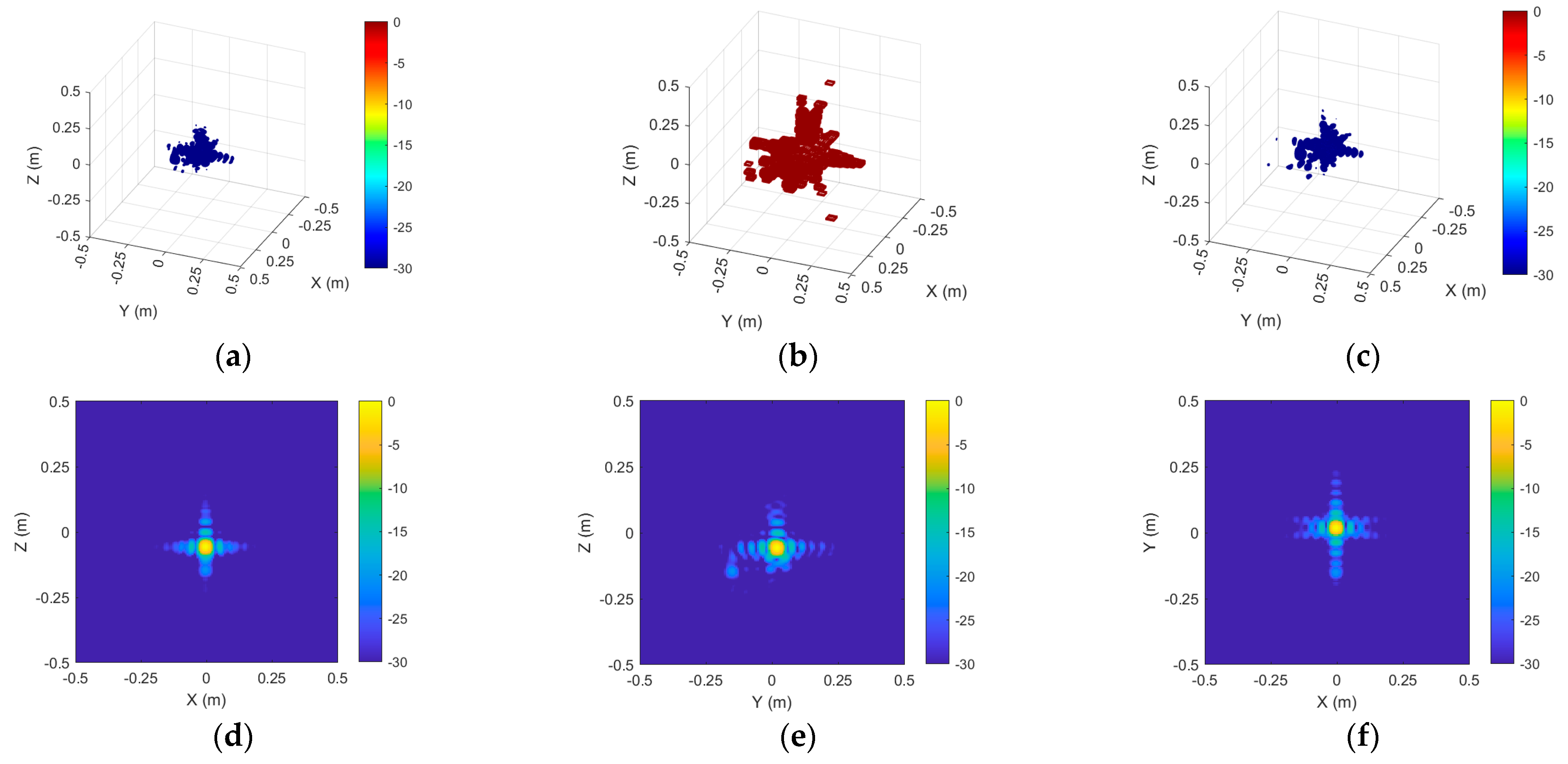
5.2.1. Sphere 1

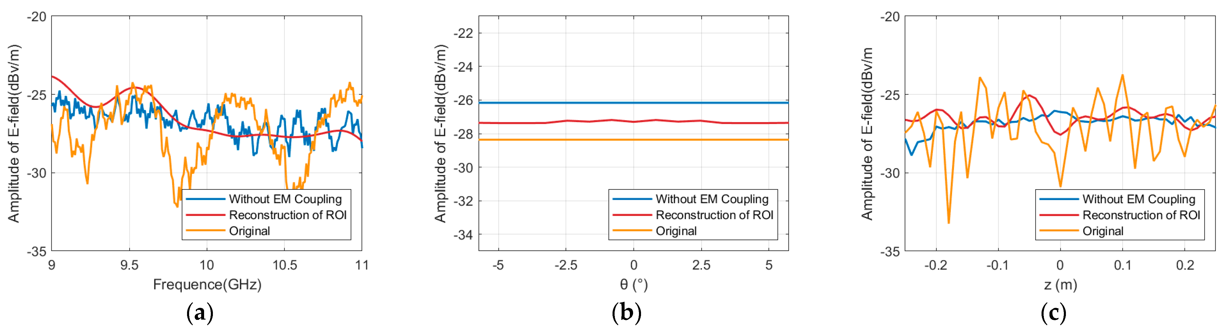
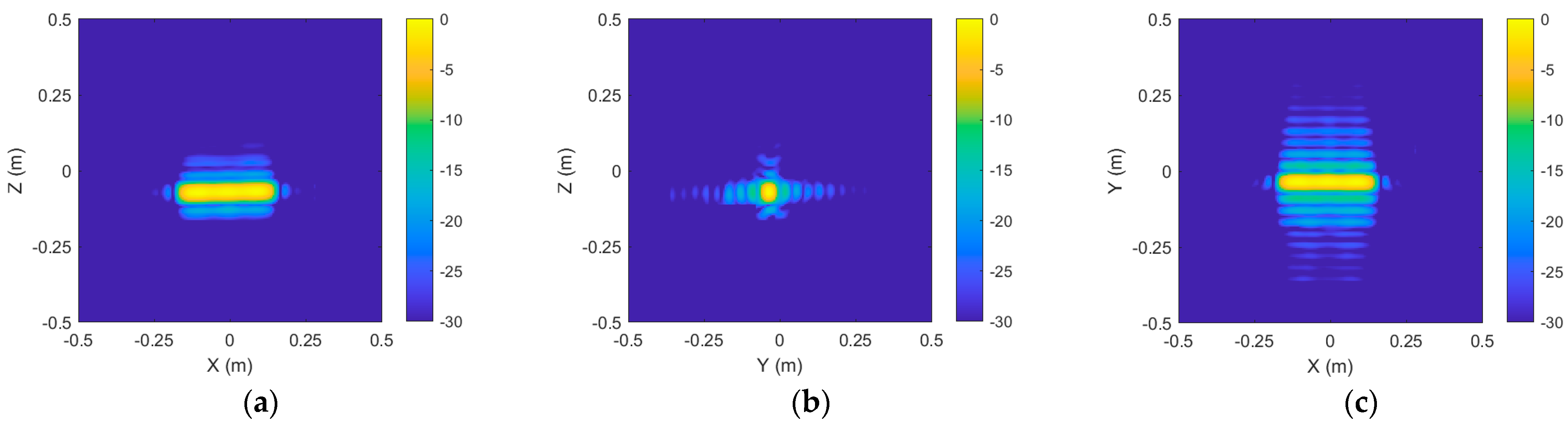
To further analyze the local scattering characteristics of the target, the results of the extracted region of interest (ROI) are shown in Figure 10. The distribution of the main scattering points within Sphere 1 is presented from different viewing angles in the figure. After applying coupling scattering suppression, the ROI echo reconstruction results of Sphere 1 are shown in Figure 11.

Following the elimination of coupling scattering sources, the near-field echo data of the region of interest were rebuilt utilizing 3D imaging. In comparison to direct measurement, the frequency domain error diminished from 1.46 dB to 0.89 dB, the angular domain error declined from 0.36 dB to 0.08 dB, and the vertical domain error decreased from 1.51 dB to 0.62 dB.

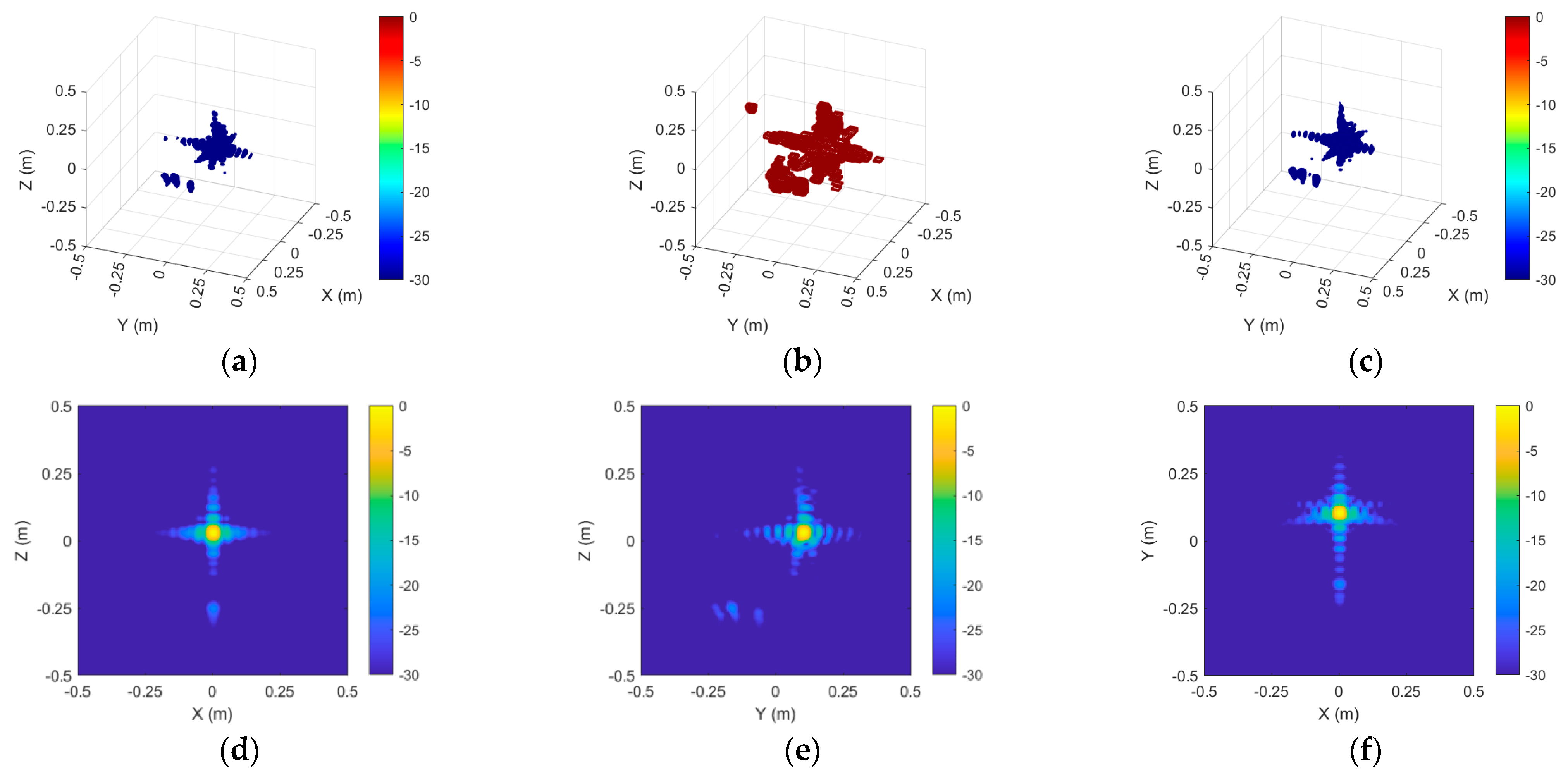
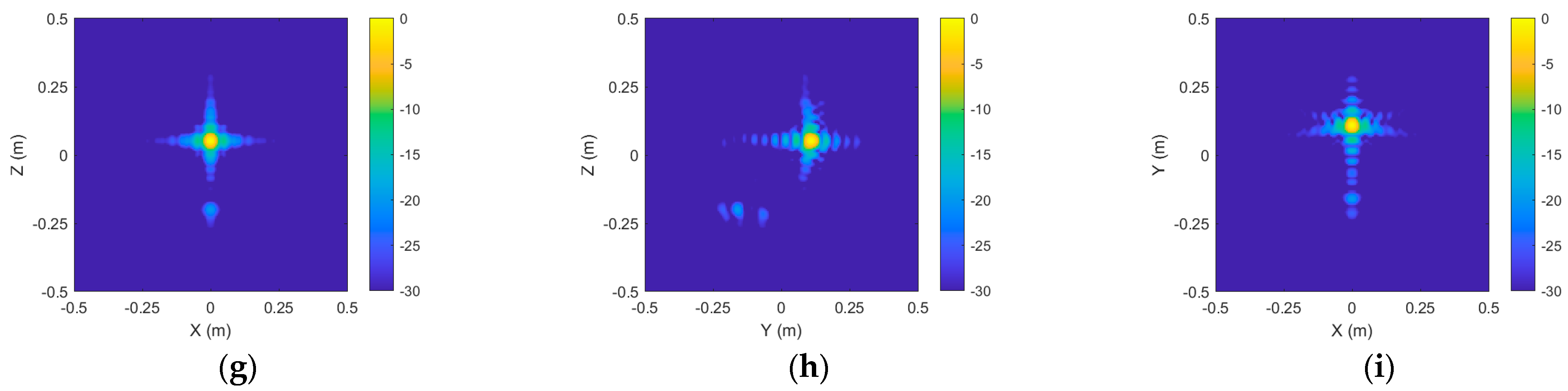
5.2.2. Sphere 2

For the large-sized target Sphere 2, the ROI imaging results are presented in Figure 12. Figure 13 displays the echo reconstruction results of Sphere 2 after the suppression of background coupling.

In comparison to Target 1, enlarging the metallic sphere leads to an increased inherent dispersion of the target. As a result, the target–background coupling scattering also intensifies, further enhancing its effect on the total scattering properties. Following the elimination of coupling scattering sources, the near-field echo data of the region of interest were rebuilt utilizing 3D imaging. In comparison to direct measurement, the frequency domain error diminished from 2.81 dB to 1.38 dB, the angular domain error declined from 2.14 dB to 0.97 dB, and the vertical domain error decreased from 2.96 dB to 1.22 dB.

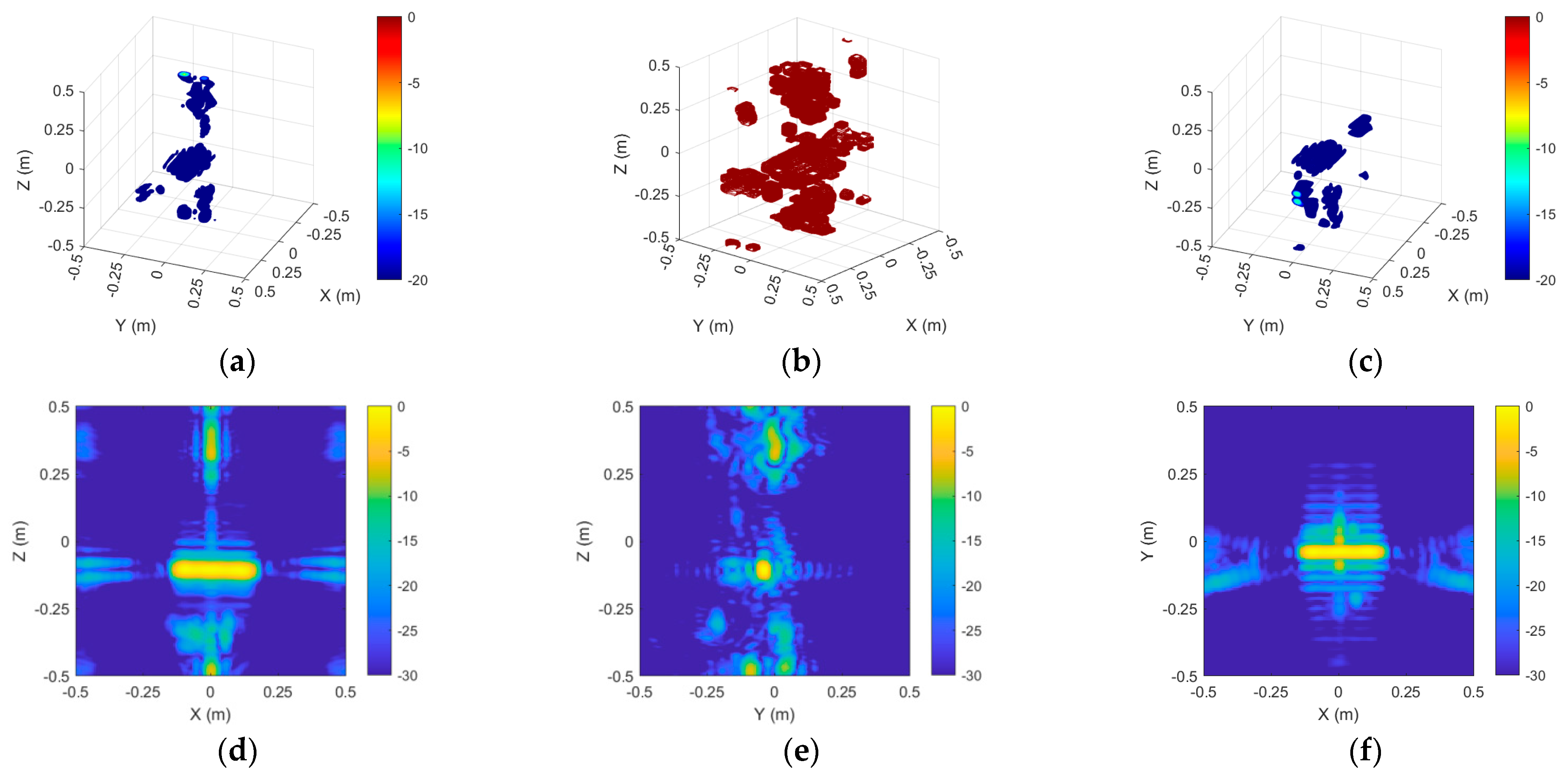
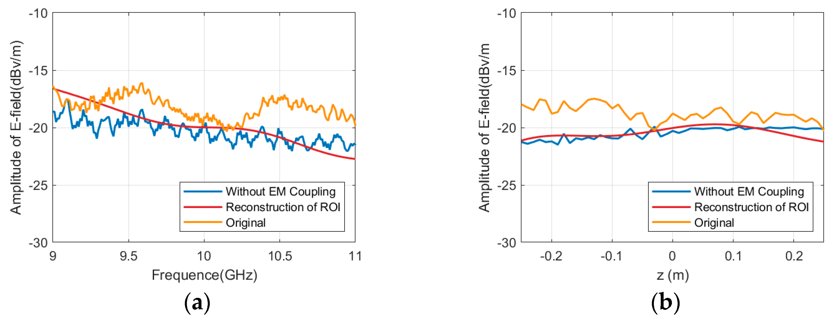
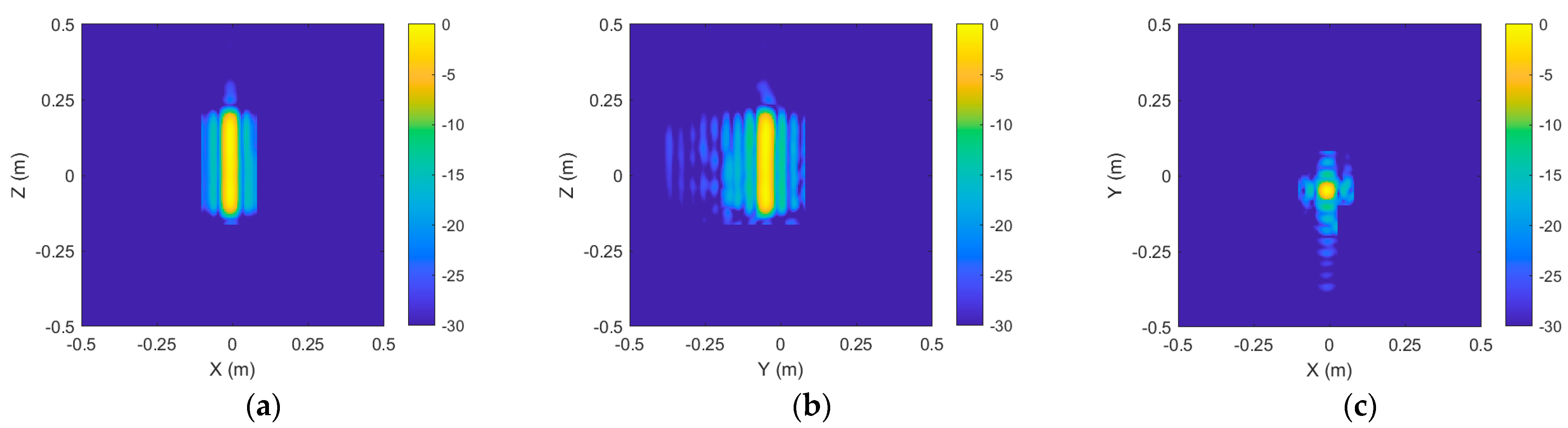
5.2.3. Cylinder

For the cylindrical target, the ROI imaging results are presented in Figure 14. Figure 15 displays the echo reconstruction results of the cylindrical target’s ROI after processing.

Following the elimination of coupling scattering sources, the near-field echo data of the region of interest were rebuilt utilizing 3D imaging. In comparison to direct measurement, the frequency domain error diminished from 2.04 dB to 1.15 dB, and the vertical domain error decreased from 1.75 dB to 0.21 dB. The echo reconstruction results for Sphere 1, Sphere 2, and the Cylinder indicate that the proposed algorithm enhances the test accuracy by removing the coupling scattering sources between the targets and the background.

5.2.4. Two Cylinders

To eliminate the effects of interference targets and coupled scattering, Cylinder 1 is extracted as the ROI region from the imaging results of the double-cylinder target, as shown in Figure 16. The echo reconstruction results are presented in Figure 17. By isolating the center cylindrical region from two cylinders as the ROI and reconstructing the near-field scattering echoes for the ROI, the errors were markedly diminished in comparison to the direct measurement of the complete structure. The frequency domain error diminished from 2.91 dB to 1.02 dB, the angular domain error declined from 5.88 dB to 1.01 dB, and the vertical domain error was lowered from 3.01 dB to 1.39 dB. This outcome further illustrates the efficacy of the proposed algorithm in reconstructing echoes from scattering sources inside designated ROI zones.

6. Conclusions

This paper investigates an enhanced methodology for quantifying radar target near-field scattering properties through a 3D imaging algorithm designed for circular scanning. A hybrid methodology integrating wavenumber domain and time domain methodologies is presented to rectify the computational inefficiencies inherent in traditional 3D BP imaging algorithms. The suggested method attains a compromise between the computational economy and image precision by incorporating quick scattering source extraction and exact computing in important areas.

The experimental results indicate that the proposed technique markedly enhances the imaging speed and accuracy, substantially decreasing the calculation time while preserving the high precision necessary for near-field scattering measurements. The approach effectively reconstructs near-field echoes from scattering sources, demonstrating its capability to decouple target–background interactions. Furthermore, the adaptability of this method broadens its use to diverse imaging geometries, such as planar and spherical sampling, underscoring its versatility in sophisticated radar imaging systems.

Future endeavors will concentrate on augmenting the algorithm’s processing efficiency to accommodate more intricate scenarios and larger datasets. Furthermore, the research will focus on enhancing the identification and differentiation of linked scattering sources in 3D imaging. In addition to positional information, alternative approaches for identifying coupled scattering sources, including scattering mechanism analysis and frequency domain characteristics, will be investigated to enhance decoupling capabilities, thereby advancing radar imaging and scattering research. Future research may focus on the applicability of complex models that incorporate multiple scattering sources and various scattering mechanisms, along with the estimation of a remote target Radar Cross Section (RCS) derived from near-field echo inversions.