Assessment of the Potential of Spaceborne GNSS-R Interferometric Altimetry for Monthly Marine Gravity Anomaly

Abstract

The Earth’s time-variable gravity field holds significant research and application value. However, satellite gravimetry missions such as GRACE and GRACE-FO face limitations in spatial resolution when detecting monthly gravity fields, while traditional radar altimeters lack the observational efficiency needed for monthly gravity anomaly inversion. These limitations hinder further exploration and application of the Earth’s time-variable gravity field. Leveraging its advantages, such as rapid global coverage, high revisit frequency, and low cost for constellation formation, spaceborne GNSS-R technology holds the potential to address the observational efficiency gaps of traditional radar altimeters. This study presents the first assessment of the capability of spaceborne GNSS-R interferometric altimetry for high spatial resolution monthly marine gravity anomaly inversion through simulations. The results indicate that under the PARIS Operational scenario of a single GNSS-R satellite (a spaceborne GNSS-R interferometric altimetry scenario proposed by Martin-Neira), a 30′ grid resolution marine gravity anomaly can be inverted with an accuracy of 4.93 mGal using one month of simulated data. For a dual-satellite constellation, the grid resolution improves to 20′, achieving an accuracy of 4.82 mGal. These findings underscore the promise of spaceborne GNSS-R interferometric altimetry technology for high spatial resolution monthly marine gravity anomaly inversion.

1. Introduction

The Earth’s gravitational field is a vital physical quantity in Earth sciences, providing valuable insights into the Earth’s mass distribution, density, and internal structure. Its spatio-temporal variations enable us to understand and track dynamic processes of material transport and exchange within the Earth’s system [1]. With approximately 71% of the Earth’s surface covered by oceans, the recovery of marine gravity field is essential for building a comprehensive Earth gravity field model. The time-variable marine gravity field is crucial for studying changes in the Earth’s system and engineering applications, such as the water cycle, climate change, movement of materials within the Earth, and energy development [2]. Additionally, the higher the resolution of the marine time-variable gravity field, the more information it provides about dynamic processes in the Earth’s system. Therefore, obtaining high-resolution, time-varying information about the marine gravity field is essential for both research and applications in Earth sciences.

In 1969, Wolff proposed the GRACE mission concept, employing inter-satellite ranging measurements between two low Earth co-orbiting satellites to observe the Earth’s time-variable gravity field [3]. At present, GRACE/GRACE-FO serve as the primary tools for detecting the global gravity variation, having continuously provided the monthly Earth’s gravity field data for over two decades [4]. These missions have significantly advanced the monitoring and understanding of global environmental changes, encompassing variations in ground-water storage [5], deformation caused by earthquakes [6], sea level rise [7], deep ocean currents [8], and ocean heat content [9]. However, the orbital configuration of GRACE/GRACE-FO satellites (~500 km satellite altitude, ~220 km inter-satellite distance) fundamentally limits the spatial resolution of their derived time-variable gravity fields to hundreds of kilometers [10]. Furthermore, the accuracy of the gravity field degrades significantly with increasing spherical harmonic degree, as high-degree coefficients dominated by noise [11]. To mitigate the impact of strong longitudinal stripes and random noises, spatial filtering is required, further reducing the spatial resolution of GRACE/GRACE-FO time-variable gravity data [12]. Currently, the monthly gravity field products from GFZ GRACE Release 06 (RL06) solutions are truncated at spherical harmonic degrees of 60 and 96 [13], corresponding to spatial resolutions of approximately 330 km and 220 km (half-wavelength) [14], respectively. Consequently, the coarse spatial resolution of the gravity field products provided by GRACE/GRACE-FO satellites hinders further research and applications of time-variable gravity fields [15,16].

Marine gravity anomalies from satellite altimetry have greatly improved the accuracy and spatial resolution of static marine gravity anomaly results [17,18,19,20], allowing for a better understanding of deep-sea seabed topography and structure [21,22,23]. However, due to the satellite’s limited view confined to the nadir and the high cost of constructing large-scale constellations, traditional radar altimeters struggle to achieve rapid global coverage and revisiting capabilities [24]. As a result, radar altimeter data are mainly used for inverting static marine gravity anomaly rather than for time-variable marine gravity fields, due to their insufficient observational efficiency. In 2021, Li et al. first utilized the yearly marine time-variable gravity field from radar altimetry, revealing the undersea volcano magma mass motions of the Izu-Bonin arcs near Japan. However, it was also pointed out that the low time resolution of altimetry-derived marine time-variable gravity fields makes it challenging to study rapidly evolving volcanic systems [25]. In 2023, Guo et al. verified the feasibility of deriving high spatial resolution monthly marine time-variable gravity anomaly from CryoSat-2 altimetry data. However, there may be no data within the window when the calculation window was less than 60′. Therefore, despite the resulting grid resolution for the monthly marine time-variable gravity anomaly being 3′, a 60′ calculation window was used due to insufficient data from the radar altimeter, leading to a poor overall resolution [26].

The spaceborne Global Navigation Satellite System Reflectometry (GNSS-R) is a passive remote sensing technique that can receive multiple reflected signals from GNSS satellites simultaneously, covering wide swathes. This allows for advantages such as large data volume, low power consumption, low cost for constellation formation, and rapid global coverage and revisiting capabilities [27]. Figure 1 shows the diagram of spaceborne GNSS-R observations. The concept of utilizing GNSS reflections for remote sensing was initially proposed by Hall in 1988 [28] and later expanded by Martin-Neira in 1993 with the PARIS concept (Passive Reflectometry and Interferometry System), which combines GNSS direct and reflected signals for altimetry [29]. At present, multiple spaceborne GNSS-R missions are in orbit [30,31,32,33,34,35], and have been successfully applied in various fields such as sea surface wind speed [36,37], sea ice [38,39], and soil moisture [40,41]. Sea surface height (SSH) altimetry is one of the most promising and challenging applications of GNSS-R, which can complement existing technologies such as radar satellites [42]. However, spaceborne GNSS-R altimetry technology still faces many challenges in practical applications. On one hand, most existing Spaceborne GNSS-R missions do not specifically target SSH altimetry; the altimetry accuracy is relatively poor due to the use of low bandwidth signals [43,44,45]. On the other hand, although carrier-phase altimetry experiments on PRETY and Spire satellites have achieved centimeter-level precision, the stringent observation conditions and insufficient effective observation rates remain significant challenges [46,47,48,49].

The spaceborne GNSS-R interferometric processing technique, proposed by Martin-Neira in 2011, is currently considered to be the most feasible spaceborne altimetry mode for spaceborne GNSS-R altimetry. By incoherently integrating power waveforms from multiple samples, the proposed PARIS IOD and Operational spaceborne GNSS-R missions can achieve decimeter-level sea surface height measurements with a 100-km along-track spatial resolution [50]. Subsequent studies have confirmed the stable performance of spaceborne GNSS-R interferometric altimetry in both accuracy and observation efficiency [51,52]. Meanwhile, the European Space Agency (ESA) proposed the GEROS-ISS mission [53], which, although not yet implemented, has significantly advanced GNSS-R interferometric altimetry. In 2016, Martin-Neira introduced the “Cookie” satellite constellation concept, analyzing its potential for networked observations [27]. Additionally, the feasibility of near real-time target detection from a constellation of GNSS-R has been demonstrated [54], offering even better temporal resolution than SWOT in mesoscale ocean observations [55]. This technology has shown significant potential for ocean circulation monitoring, positioning it as a valuable complement to traditional radar altimetry [56]. Furthermore, scholars also have pointed out that GNSS-R SSH altimetry products will become an important data source for global marine gravity anomaly inversion [57,58].

However, detecting short-wavelength marine gravity fields requires higher altimetry spatial resolution, yet increasing the GNSS-R along-track spatial resolution reduces the number of incoherent integrations, thereby decreasing altimetric accuracy. In 2018, Li et al. systematically analyzed the impact of incoherent integration and post-integration waveforms on the accuracy of interferometric altimetry [59]. Furthermore, studies indicate that the minimum spatial resolution of spaceborne GNSS-R altimetry footprints is approximately 10 km [55]. In 2024, our previous work demonstrated through simulations that PARIS can achieve high-precision inversion of marine vertical deflection (referred to as the deflection of vertical, DOV, another parameter for describing the gravity field) with a 10 km along-track resolution. Moreover, it is further speculated that its global coverage and revisit capabilities may contribute to the inversion of high-spatial resolution marine time-variable gravity fields [60].

Based on our previous work [60], this paper aims to assess the potential contribution of spaceborne GNSS-R interferometric altimetry technology in improving the current spatial resolution and accuracy of marine time-variable gravity fields. Specifically, it evaluates the precision of global monthly marine gravity anomaly inversion using one month of simulated data at various resolutions. Additionally, the impact of dual-satellite constellation observations and different instrument configurations on the accuracy of monthly marine gravity anomaly inversion will be analyzed.

2. Experimental Data

To simulate spaceborne GNSS-R SSH interferometric altimetry data, the GNSS-R specular point trajectory data from the FY-3E and FY-3F satellites were utilized as input. The FY-3E and FY-3F satellites were launched in July 2021 and August 2023, respectively, and have formed a three-satellite constellation observation with the FY-3G satellite, which was launched in April 2023 [61]. All of these satellites carry the GNOS-II payload, which is capable of receiving GNSS reflection signals from the earth’s surface through eight signal-receiving channels, including GPS, BDS, and GALILEO. However, compared to the FY-3G satellite with an orbital altitude of 407 km and an inclination angle of 50°, the FY-3E and FY-3F satellites are more ideal for global SSH observations with an orbital altitude of 836 km and an inclination angle of 98.75°, aligning with the orbit parameters of geodetic missions. Therefore, the Level 2 (L2) GNSS-R specular points trajectory of FY-3E/F satellites in October 2023 are utilized to evaluate the ability to detect global monthly marine gravity anomalies through spaceborne GNSS-R interferometry altimetry.

Figure 2 displays the daily trajectory map of specular points for FY-3E and FY-3F. It can be observed that the specular points trajectories of these two satellites are adjacent, which allows them to complement each other and improve the coverage of spaceborne GNSS-R through constellation observation. In addition, due to strict data control and filtering of L2 data, the number of observation strips of each satellite does not always reach the maximum observable number. After calculation, in the selected L2 data for October 2023, FY-3E satellite utilized an average of 3.5 channels out of 8 channels, while FY-3F utilized an average of 3.8 channels.

In recent years, spaceborne GNSS-R interferometric altimetry performance and methodologies have been extensively studied and optimized. However, the PARIS interferometric altimetry performance model proposed by Martin-Neira (2011) remains the most classic and representative achievement in this field [50]. Therefore, this study adopts it as the theoretical foundation and a typical representation of GNSS-R interferometric altimetry performance. According to the error budget table analyzed by Martin-Neira, the antenna gain for PARIS in IOD and Operational scenarios are 23 dBi and 30 dBi, respectively, with orbital altitudes of 800 km and 1500 km. After incoherently integrating power waveforms from multiple samples and considering correction accuracies for instrument noise, ionosphere, troposphere, electromagnetic bias, skewness bias, and orbit, the altimetry accuracy can reach 17.5 cm and 7.5 cm at the edge of a swath with a 100 km along-track resolution. This altimetric performance can meet the detection requirements of its main target of ocean mesoscale studies.

To meet the detection requirements for high-frequency information of gravity field, the minimum along-track resolution (10 km) achieved by spaceborne GNSS-R interferometric altimetry should be taken as the parameter. Based on the altimetry accuracy proposed by Martin-Neira for a 100 km along-track resolution and its relationship with along-track resolution, the altimetry accuracy for the IOD and Operational scenarios at a 10 km along-track resolution can be extrapolated. Additionally, Martin-Neira’s error budget table omits the impact of geophysical error corrections such as tide correction and inverted barometer correction, which are crucial for gravity field inversion. Referring to the geophysical correction error budgets of radar altimeters, this study sets the correction accuracy for geophysical errors at 3 cm [62]. Furthermore, the orbital altitude of FY-3E/F differs from that of PARIS IOD and Operational scenarios, and orbital altitude significantly affects the detection efficiency and altimetry accuracy of GNSS-R. Therefore, this study recalculated the altimetry accuracy of PARIS based on the error budget table proposed by Martin-Neira, taking into account the impact of the orbital altitude of FY-3E/F, 10 km along-track resolution, and geophysical error correction. The results showed that at the orbit altitude of FY-3E/F, the altimetry accuracy for IOD ${\sigma }_{IOD}$ and Operational scenarios ${\sigma }_{Operational}$ are 41.52 cm and 16.17 cm, respectively, with a 10 km along-track resolution. Figure 3 illustrates the process of simulating spaceborne GNSS-R altimetry data, while the detailed calculation process can be found in our previous work [60].

Prior to simulating sea surface height (SSH) data for spaceborne GNSS-R interferometric altimetry, sparse sampling was applied to the specular point trajectory data of the FY-3E and FY-3F satellites. This approach was adopted to address the 5.6 km ground spacing between adjacent along-track specular points of FY-3E/F satellites, which is below the minimum achievable along-track resolution (10 km) for spaceborne GNSS-R interferometric altimetry. The sparse sampling ensures the independence between adjacent sampling points along the track, thereby eliminating data redundancy. As shown in Figure 4, the minimum sampling distance was set at 10 km.

To simulate SSH in spaceborne GNSS-R interferometric altimetry, the DTU21MSS model from the Technical University of Denmark (DTU) was selected as the input mean sea surface (MSS) model. With a grid resolution of 1 arc-minute, the DTU21MSS model is significantly finer than the 10 km spatial resolution achievable by spaceborne GNSS-R interferometric altimetry, except in polar regions. To accurately represent the impact of the spatial resolution of spaceborne GNSS-R interferometry on the SSH observations, the average SSH within the spatial resolution of spaceborne GNSS-R interferometry was employed as the background field. As shown in Figure 4, a 10 km × 10 km specular reflection area was constructed with each spaceborne GNSS-R specular point as the center, and the reflection area was resampled into points with a 2 km interval. The SSH value at each resampling point within the reflection area was calculated by interpolating with the DTU21MSS model, and the average SSH of all resampling points within the reflection area was calculated as the average MSS within the specular reflection area $MS{S}_{Sp\_area}$.

At a single point, the altimetry accuracy can also be seen as the difference error between spaceborne GNSS-R SSH interferometric altimetry results and the true SSH. Furthermore, in practical scenarios, the altimetry errors of adjacent points along the track are generally correlated. However, from a global and long-term observation perspective, the distribution of all altimetry errors follows a normal distribution. Therefore, in the evaluation of the global monthly marine gravity field recovered by spaceborne GNSS-R interferometric altimetry, altimetry errors can be assigned to all points based on the central limit theorem. This is achieved by generating a random number from a normal distribution with a mean of 0 and a standard deviation of altimetry accuracy (41.52 cm for the IOD scenario and 16.17 cm for the Operational scenario). Lastly, the final simulated results of spaceborne GNSS-R interferometric altimetry results $SS{H}_{GNSS-R}$ will be determined by adding altimetry errors ${\epsilon }_{altimetry}$ to the $MS{S}_{Sp\_area}$.

$$SS{H}_{GNSS-R}=MS{S}_{Sp\_area}+{\epsilon }_{altimetry}=SS{H}_{MSS}+{\epsilon }_{area}+{\epsilon }_{altimetry}$$

(1)

where $SS{H}_{MSS}$ represents the sea surface height at the center point of the GNSS-R specular reflection, while ${\epsilon }_{area}$ denotes the difference between the mean sea surface height $MS{S}_{Sp\_area}$ within the GNSS-R altimetry resolution and $SS{H}_{MSS}$. The difference ${\epsilon }_{area}$ reflects the impact of GNSS-R altimetry resolution on the altimetry results and is referred to as the representativeness error in the [55].

Figure 5 provides an example of the simulated SSH altimetry results for an Operational track. Figure 5b shows the variations of the simulated Operational SSH altimetry results and the true SSH (using the MSS as the true SSH) along the red track in Figure 5a, while Figure 5c displays the differences between the simulated Operational SSH altimetry results and the true SSH. It can be observed that the simulated Operational SSH $SS{H}_{Operational}$ follows a similar trend as the true sea surface height $SS{H}_{MSS}$, but with an error term compared to the true SSH. As shown in Figure 5c, the error term corresponds to the simulated spaceborne GNSS-R interferometric altimetry error, which includes both representativeness errors ${\epsilon }_{area}$ and altimetric errors ${\epsilon }_{altimetry}$.

3. Methodology

The inverse Vening Meinesz method is a commonly used method for gravity anomalies inversion using vertical deflections. Therefore, prior to calculating the gravity anomalies, the gridded vertical deflection components must first be derived from the simulated spaceborne GNSS-R SSH altimetry results in Section 2. Additional filtering was applied to the simulated data, removing points with errors greater than 3 times the value of the altimetry accuracy $\sigma$. Since the gravity anomaly inversion relies on the geoid height N, where $N=MSS-DTU$, the MDT_CNES_CLS_18_global model obtained from AVISO was subtracted from the simulated SSH to eliminate the influence of mean dynamic topography (MDT) and obtain the simulated geoid height. The gridded geoid surface is then obtained by gridding the geoid heights of all simulated altimetry points in a month. Finally, the vertical deflection on the grid (i,j) can be calculated using Equations (2) and (3) for the north–south ξ(i,j) and east–west directions $\eta$(i,j), respectively. This algorithm not only improves efficiency but has also been verified for accuracy and applicability [63,64].

$$\xi \left(i,j\right)=-{\displaystyle \frac{1}{R}}{\displaystyle \frac{\left(N_{i+1}-N_i\right)}{\left({\phi }_{i+1}-{\phi }_i\right)}}$$

(2)

$$\eta \left(i,j\right)=-{\displaystyle \frac{1}{Rcos{\phi }_i}}{\displaystyle \frac{\left(N_{j+1}-N_j\right)}{\left({\lambda }_{j+1}-{\lambda }_j\right)}}$$

(3)

where $R$ is the Earth’s mean radius, $N$ is the mean geoid height at the grid point, and $\phi$ and $\lambda$ represent the latitude and longitude of the grid point, respectively.

In 1997, Hwang derived the Inverse Vening Meinesz formula, which converts vertical deflections into gravity anomalies by utilizing the gradient of the H function, as Equations (4) and (5).

$$\Delta \mathrm{g}(p)={\displaystyle \frac{{\gamma }_0}{4\pi }}{\displaystyle {\iint }_{\sigma }{H}^{\prime }({\xi }_q\cos {\alpha }_{qp}+{\eta }_q\sin {\alpha }_{qp})d{\sigma }_q}$$

(4)

$$H^{\prime }={\displaystyle \frac{\mathrm{d}H}{d{\psi }_{pq}}}=-{\displaystyle \frac{\cos \frac{{\psi }_{pq}}{2}}{2{\sin }^2\frac{{\psi }_{pq}}{2}}}+{\displaystyle \frac{\cos \frac{{\psi }_{pq}}{2}\left(3+2\sin \frac{{\psi }_{pq}}{2}\right)}{2\sin \frac{{\psi }_{pq}}{2}\left(1+\sin \frac{{\psi }_{pq}}{2}\right)}}$$

(5)

where the average gravity of the Earth ${\gamma }_0={\displaystyle \frac{GM}{R^2}}$, $H^{\prime }$ is the gradient of the H function, and p and q are two points on the sphere. ${\alpha }_{qp}$ and ${\psi }_{pq}$ represent the azimuth and spherical distance between the two points and can be calculated using Equations (6) and (7).

$$\tan {\alpha }_{qp}={\displaystyle \frac{-\cos {\varphi }_p\sin \Delta {\lambda }_{qp}}{-\sin \left({\varphi }_q-{\varphi }_p\right)+2\sin {\varphi }_q\cos {\varphi }_p{\sin }^2\frac{\Delta {\lambda }_{qp}}{2}}}$$

(6)

$${\sin }^2\left({\displaystyle \frac{{\psi }_{qp}}{2}}\right)={\sin }^2\left({\displaystyle \frac{\Delta {\varphi }_{qp}}{2}}\right)+{\sin }^2\left({\displaystyle \frac{\Delta {\lambda }_{qp}}{2}}\right)\cos {\varphi }_q\cos {\varphi }_p$$

(7)

where $\Delta {\varphi }_{qp}={\varphi }_q-{\varphi }_p$, $\Delta {\lambda }_{qp}={\lambda }_q-{\lambda }_p$, ${\varphi }_p$ and ${\varphi }_q$ represent the latitude of points p and q, while ${\lambda }_p$ and ${\lambda }_q$ represent the longitude of point p and q.

Additionally, Hwang considered latitude differences and used a one-dimensional Fast Fourier Transform (1D FFT) for global gravity field calculations, making the theoretical framework more rigorous:

$$\begin{array}{l}\Delta g_{{\varphi }_p}\left({\lambda }_p\right)={\displaystyle \frac{{\gamma }_0\Delta \varphi \Delta \lambda }{4\pi }}{\displaystyle \sum _{{\varphi }_q={\varphi }_1}^{{\varphi }_n}{\displaystyle \sum _{{\lambda }_q={\lambda }_1}^{{\lambda }_n}{H}^{\prime }\left(\Delta {\lambda }_{qp}\right)\times \left({\xi }_{\cos }\cos {\alpha }_{qp}+{\eta }_{\cos }\sin {\alpha }_{qp}\right)}}\\ ={\displaystyle \frac{{\gamma }_0\Delta \varphi \Delta \lambda }{4\pi }}{F}_1^{-1}\times \left\{{\displaystyle \sum _{{\varphi }_q={\varphi }_1}^{{\varphi }_n}\left[F_1\right.}\left(H^{\prime }\left(\Delta {\lambda }_{qp}\right)\cos {\alpha }_{qp}\right)F_1\left({\xi }_{\cos }\right)\right.\\ +\left.F_1\left(H^{\prime }\left(\Delta {\lambda }_{qp}\right)\sin {\alpha }_{qp}\right)F_1\left({\eta }_{\cos }\right)\right\}\end{array}$$

(8)

where ${\xi }_{\cos }=\xi \cos \varphi$, ${\eta }_{\cos }=\eta \cos \varphi$, and $\Delta \varphi$ and $\Delta \lambda$ represent the grid spacing in the latitude and longitude directions, respectively.

However, when the spherical distance ${\psi }_{pq}=0$, the kernel function will be singular. Therefore, the innermost zone effect must be considered, which can be calculated using Equation (9):

$$g_0={\displaystyle \frac{s_0{\gamma }_0}{2}}\left({\xi }_y+{\eta }_x\right)$$

(9)

$${\mathrm{s}}_0={\left({\displaystyle \frac{\Delta \varphi \Delta \lambda }{\pi }}\right)}^{{\displaystyle \frac{1}{2}}}$$

(10)

where ${\mathrm{s}}_0$ is the innermost zone, ${\xi }_y={\displaystyle \frac{\partial \xi }{\partial y}}$, and ${\eta }_x={\displaystyle \frac{\partial \eta }{\partial x}}$.

It should be noted that the grid DOV calculated from the simulated data is only available for the marine region. However, since the gravity of the land area also affects the long-wave component of the marine gravity field, the DOV resolved by the EGM2008 model is used to fill the missing values in the land area before calculating the marine gravity anomaly. It can be seen that we did not use the remove–restore method to restore the long-wave component of the marine gravity field for the residual gravity anomalies [19], but instead used the total vertical deflection to invert the gravity anomalies. While both methods aim to recover the long-wave component of the gravity field, the remove–restore method is unable to effectively suppress noise in the simulation scenarios. On the other hand, using total vertical deflection for gravity anomaly inversion allows for a better assessment of the potential of utilizing spaceborne GNSS-R interferometric altimetry in simulation gravity field inversion.

Lastly, the gravity anomaly model EGM2008, released by the National Geospatial-Intelligence Agency (NGA), is employed as the true gravity anomaly values. These reference values are then compared with the gravity anomaly results calculated using the simulated data in a month. The EGM2008 model provides up to 2159 degrees and 2190 orders of spherical harmonic coefficients, which can be used to calculate gravity anomaly results with a spatial resolution of up to 5′ × 5′ using spherical harmonic functions, as shown in Figure 6. By using different maximum spherical harmonic coefficients for expansion orders, we can obtain gravity anomaly results with different grid resolutions and compare them with the simulated gravity anomaly results at corresponding resolutions. The relationship between the order of maximum spherical harmonic coefficients and spatial resolution can be described by Equation (11):

$$\Omega ={180}^{\circ }/n$$

(11)

where n is the maximum degree of the spherical harmonic coefficients used, and $\Omega$ is the corresponding resolution of the model.

4. Results and Discussion

4.1. Assessment of Monthly Marine Gravity Field Recovered a Single GNSS-R Satellite

To explore the feasibility of using spaceborne GNSS-R interferometric altimetry for monthly marine gravity anomaly inversion, this study first simulated GNSS-R SSH interferometric altimetry data based on one-month trajectories from the FY-3E satellite and then inverted the monthly global marine gravity anomaly within latitudes between ±80°. Based on our previous research, spaceborne GNSS-R has the advantages of rapid coverage and revisits, which can compensate for the poor accuracy of single altimetry and obtain high-precision global marine vertical deflections. As the accuracy of vertical deflections directly affects the accuracy of gravity anomaly inversion, it can be expected that altimetry accuracy and revisits are also important factors affecting the accuracy of marine gravity anomaly inversion using spaceborne GNSS-R interferometric altimetry. Altimetry accuracy depends on instrument performance and error correction accuracy, which can be demonstrated through simulations using PARIS IOD and Operational scenarios. When the time period is fixed to one month, the size of the grid used is the key factor affecting the number of revisits. Therefore, the accuracy of monthly gravity anomaly simulations was evaluated for grid sizes of 10′, 15′, 20′, 25′, and 30′ under both PARIS IOD and Operational scenarios. The results are shown in

Table 1. Evaluation of monthly gravity anomaly simulation for single PARS IOD and Operational satellite with different grid resolution.

Grid Resolution	Scenarios	Mean (mGal)	RMS (mGal)	Coverage Rate	Revisits
10′	IOD	−0.06	28.37	72.62%	2.34
	Operational	0.05	13.22
15′	IOD	−0.06	14.34	84.31%	5.27
	Operational	−0.07	8.09
20′	IOD	−0.08	8.98	89.83%	9.39
	Operational	−0.08	6.15
25′	IOD	−0.09	6.77	91.14%	14.68
	Operational	−0.09	5.36
30′	IOD	−0.10	5.70	91.91%	21.14
	Operational	−0.11	4.93

, which reflects the ability of spaceborne GNSS-R interferometric altimetry to invert monthly marine gravity anomaly.

According to Table 1, at a grid resolution of 10′, the inversion accuracy is poor in both the IOD and Operational scenarios, at 28.37 mGal and 13.22 mGal, respectively. The superior accuracy of the Operational scenario highlights its advantage over the IOD scenario, primarily due to the insufficient coverage rate (72.62%) and low average revisits (2.34 times) of a single spaceborne GNSS-R satellite at this resolution. However, in the Operational scenario, the inversion accuracy reaches within 10 mGal at a grid resolution of 15′ or finer, and within 5 mGal at a grid resolution of 30′, specifically 4.93 mGal. In the IOD scenario, the accuracy reaches within 10 mGal at a grid resolution of 20′ or finer. In conclusion, the accuracy of monthly gravity field inversion is significantly influenced by the accuracy of GNSS-R interferometric altimetry under the observation of a single satellite.

Furthermore, Guo et al. used CryoSat-2 conventional radar altimeter data to successfully invert the monthly gravity anomaly, achieving an accuracy of 5.063 mGal with a 60′ search radius [26]. Comparing this to the Operational scenario’s inversion accuracy of 4.93 mGal at a grid resolution of 30′, and the IOD scenario’s accuracy of 5.7 mGal, it can be seen that the inverted gravity field from spaceborne GNSS-R interferometric altimetry can achieve comparable accuracy at a finer spatial resolution.

Figure 7 shows the 30′ monthly marine gravity anomaly inverted using simulated interferometric altimetry data from a single GNSS-R satellite in the Operational scenario. Despite some gaps in the 30′ marine gravity field, most marine areas are covered, as shown in Figure 7. According to Table 1, the coverage rate at this resolution reaches 91.91%, with an average revisit rate of 21.14. Additionally, it can be observed that there are significantly fewer detection gaps in the Indian Ocean and Western Pacific regions compared to other areas. This is due to the presence of IGSO satellites from BeiDou Navigation Satellite System (BDS-2 and BDS-3) in these regions, resulting in a higher spatial coverage range for the BDS signals received by FY-3E in these areas [65].

Additionally, it is worth noting that the coverage rate and average revisits of spaceborne GNSS-R observations increase as the grid resolution decreases, resulting in improved monthly marine gravity field inversion accuracy (RMS). Furthermore, at a grid resolution of 25′, spaceborne GNSS-R achieves a coverage rate of over 90%, specifically 91.14%, with an average of 14.68 revisits. Compared to radar altimeters, spaceborne GNSS-R offers superior global coverage due to its ability to conduct multiple track observations over the ocean. This is more efficient than traditional radar altimeters, which can only observe at nadir points. Additionally, the wide-swath observations of spaceborne GNSS-R overcomes the limitations of repetitive orbits in non-geodetic measurements, a common issue with traditional radar altimeters. Therefore, spaceborne GNSS-R interferometric altimetry has a natural advantage in high spatial resolution time-variable gravity fields compared to radar altimeters.

4.2. Assessment of Monthly Marine Gravity Field from Dual Satellite Constellation

Compared to radar altimeters, spaceborne GNSS-R payloads have the advantages of low power consumption, low weight, low cost, and low size, making them highly suitable for constellation formation [54]. Therefore, this study leverages the specular points trajectories of FY-3E and FY-3F to simulate GNSS-R interferometric altimetry data from a dual-satellite constellation for monthly marine gravity anomaly inversion. Still using a 30′ resolution as an example, Figure 8 presents the inversion results of the monthly marine gravity field in the Operational dual-satellite constellation scenario. Compared to single-satellite results, the dual-satellite constellation significantly reduces data gaps and enhances coverage.

Furthermore, the accuracy of the monthly marine gravity anomaly inversion in the dual-satellite GNSS-R interferometric altimetry constellation was evaluated, with results shown in

Table 2. Evaluation of monthly gravity anomaly simulation for PARS IOD and Operational dual-satellite constellation with different grid resolutions.

Grid Resolution	Scenarios	Mean (mGal)	RMS (mGal)	Coverage Rate	Revisits
10′	IOD	−0.04	20.35	87.83%	4.81
	Operational	0.04	9.73
15′	IOD	−0.07	9.87	91.45%	10.83
	Operational	−0.06	5.93
20′	IOD	−0.08	6.52	92.24%	19.28
	Operational	−0.08	4.82
25′	IOD	−0.09	5.22	92.46%	30.16
	Operational	−0.09	4.44
30′	IOD	−0.10	4.68	92.50%	43.43
	Operational	−0.10	4.27

. It can be observed that the dual-satellite constellation improves the coverage rate, revisits, and inversion accuracy of the monthly marine gravity anomaly compared to the single-satellite. At a 15′ grid resolution, the GNSS-R dual-satellite constellation observations can achieve a coverage rate of over 90%, reaching 91.45%, with average revisits of 10.83 times. The monthly marine gravity anomaly inversion accuracy is better than 10 mGal in both the IOD and Operational scenarios, reaching 9.87 mGal and 5.93 mGal, respectively. At a 20′ grid resolution, the accuracy in the Operational dual-satellite constellation scenario is better than 5 mGal, specifically 4.82 mGal. In the IOD scenario, at a 30′ grid resolution, the accuracy also surpasses 5 mGal, reaching 4.68 mGal. Compared to single-satellite observations, the dual-satellite constellation not only improves inversion accuracy but also narrows the accuracy gap between the IOD and Operational scenarios with increasing revisits. Therefore, GNSS-R constellations are crucial in improving the precision of monthly marine gravity anomaly inversion using spaceborne GNSS-R interferometric altimetry.

However, at 10′ grid resolution, the Operational monthly marine gravity anomaly accuracy significantly surpasses that of the IOD scenario, whether with a single satellite or a dual-satellite constellation. This is due to the fact that as spatial resolution increases, the reduction in average revisits is approximately proportional to the square of the grid resolution enhancement. For example, the average number of revisits at a 10′ grid is approximately one-fourth of that at a 20′ grid resolution. Therefore, despite high monthly revisits and accuracy of the monthly marine gravity field at a 20′ grid resolution, when inverting the monthly gravity field at higher resolutions like 10′ or 5′, the ability to enhance average revisits and improve inversion accuracy by increasing the number of networked satellites or reflection channels is limited. At this stage, the influence of altimetry accuracy becomes more pronounced.

5. Conclusions

This study utilized simulation to invert global monthly marine gravity anomalies using sea surface specular point trajectories from the FY-3E and FY-3F satellites over one month. The altimetry performance of PARIS IOD and Operational satellite GNSS-R interferometric altimetry missions, proposed by Martin-Neira, served as examples. The potential contribution of spaceborne GNSS-R interferometric altimetry to global monthly time-variable gravity field inversion was assessed based on coverage, revisit frequency, and inversion accuracy. The main conclusions are as follows:

• Spaceborne GNSS-R interferometric altimetry technology allows for high-resolution and precise inversion of monthly marine gravity anomaly, enhancing the spatial resolution of current time-variable gravity field products. In the single GNSS-R satellite Operational scenario, the accuracy of monthly marine gravity anomaly inversion on a 30′ grid can reach 4.93 mGal.
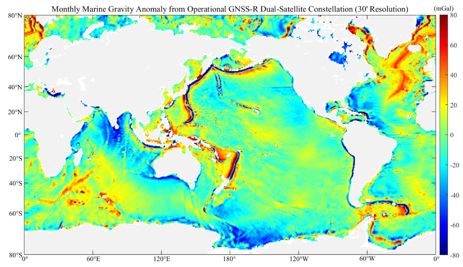
• Considering the low cost of constellation formation features of spaceborne GNSS-R technology, a dual-satellite constellation simulation experiment was conducted. The dual-satellite constellation improves the spatial resolution of time-variable gravity fields that can be inverted with the same level of accuracy. For example, in an Operational dual-satellite constellation scenario with a 5 mGal precision requirement for gravity field inversion, a dual-satellite constellation can invert a global monthly marine gravity anomaly on a 20′ grid, achieving an accuracy of 4.82 mGal.
• Increasing the number of revisits can compensate for the precision limitations of spaceborne GNSS-R interferometric altimetry, thereby enhancing the accuracy of the monthly marine gravity anomaly. It is worth noting that our study utilized only two GNSS-R satellites, each with fewer than four effective channels. Future improvements could involve increasing the number of satellites in the constellation or observation channels to enhance monthly coverage and average revisits.
• When inverting the global monthly marine gravity anomaly at a resolution finer than 10′, the precision of the inversion is significantly impacted by the accuracy of spaceborne GNSS-R interferometric altimetry. As the grid resolution improves, the need for high spatial resolution observations grows approximately proportional to the square of the grid resolution enhancement. Beyond a certain threshold, relying solely on increasing the number of satellites for network observations will also make it difficult to achieve sufficient revisits within a month. Therefore, enhancing the accuracy of spaceborne GNSS-R interferometric altimetry becomes particularly important at this stage.

In recent years, spaceborne GNSS-R technology has rapidly advanced and is expected to provide higher-quality sea surface altimetry data in the future. With advantages such as multi-track observations, low-cost constellation formation, and rapid global coverage and revisiting capabilities, it presents a promising tool for high-resolution monthly marine gravity anomaly inversion. This will complement the time-variable gravity field data from gravity satellites, advancing research and applications in Earth’s time-variable gravity fields.

References

1. Eshagh, M.; Jin, S.; Pail, R.; Barzaghi, R.; Tsoulis, D.; Tenzer, R.; Novák, P. Satellite Gravimetry: Methods, Products, Applications, and Future Trends. Earth-Sci. Rev. 2024, 253, 104783. [Google Scholar] [CrossRef]
2. Zhao, J.; Wan, J.; Sun, Q.; Liu, S. Multi-Source Ocean Gravity Anomaly Data Fusion Processing Method. In Proceedings of the IGARSS 2019—2019 IEEE International Geoscience and Remote Sensing Symposium, Yokohama, Japan, 28 July–2 August 2019; pp. 8275–8278. [Google Scholar]
3. Wolff, M. Direct Measurements of the Earth’s Gravitational Potential Using a Satellite Pair. J. Geophys. Res. 1969, 74, 5295–5300. [Google Scholar] [CrossRef]
4. Tapley, B.D.; Bettadpur, S.; Ries, J.C.; Thompson, P.F.; Watkins, M.M. GRACE Measurements of Mass Variability in the Earth System. Science 2004, 305, 503–505. [Google Scholar] [CrossRef]
5. Landerer, F.W.; Swenson, S.C. Accuracy of Scaled GRACE Terrestrial Water Storage Estimates. Water Resour. Res. 2012, 48, 2011WR011453. [Google Scholar] [CrossRef]
6. Han, S.-C.; Shum, C.K.; Bevis, M.; Ji, C.; Kuo, C.-Y. Crustal Dilatation Observed by GRACE After the 2004 Sumatra-Andaman Earthquake. Science 2006, 313, 658–662. [Google Scholar] [CrossRef]
7. Jacob, T.; Wahr, J.; Pfeffer, W.T.; Swenson, S. Recent Contributions of Glaciers and Ice Caps to Sea Level Rise. Nature 2012, 482, 514–518. [Google Scholar] [CrossRef]
8. Wahr, J.M.; Jayne, S.R.; Bryan, F.O. A Method of Inferring Changes in Deep Ocean Currents from Satellite Measurements of Time-variable Gravity. J. Geophys. Res. Oceans 2002, 107, 11-1–11-17. [Google Scholar] [CrossRef]
9. Jayne, S.R.; Wahr, J.M.; Bryan, F.O. Observing Ocean Heat Content Using Satellite Gravity and Altimetry. J. Geophys. Res. Oceans 2003, 108, 2002JC001619. [Google Scholar] [CrossRef]
10. Weigelt, M.; Sneeuw, N.; Schrama, E.J.O.; Visser, P.N.A.M. An Improved Sampling Rule for Mapping Geopotential Functions of a Planet from a near Polar Orbit. J. Geod. 2013, 87, 127–142. [Google Scholar] [CrossRef]
11. Yang, F.; Forootan, E.; Liu, S.; Schumacher, M. A Monte Carlo Propagation of the Full Variance-Covariance of GRACE-Like Level-2 Data with Applications in Hydrological Data Assimilation and Sea-Level Budget Studies. Water Resour. Res. 2024, 60, e2023WR036764. [Google Scholar] [CrossRef]
12. Vishwakarma, B.D.; Devaraju, B.; Sneeuw, N. What Is the Spatial Resolution of Grace Satellite Products for Hydrology? Remote Sens. 2018, 10, 852. [Google Scholar] [CrossRef]
13. Dahle, C.; Murböck, M.; Flechtner, F.; Dobslaw, H.; Michalak, G.; Neumayer, K.; Abrykosov, O.; Reinhold, A.; König, R.; Sulzbach, R.; et al. The GFZ GRACE RL06 Monthly Gravity Field Time Series: Processing Details and Quality Assessment. Remote Sens. 2019, 11, 2116. [Google Scholar] [CrossRef]
14. Devaraju, B.; Sneeuw, N. On the Spatial Resolution of Homogeneous Isotropic Filters on the Sphere. In Proceedings of the VIII Hotine-Marussi Symposium on Mathematical Geodesy, Rome, Italy, 17–21 June 2013; Sneeuw, N., Novák, P., Crespi, M., Sansò, F., Eds.; International Association of Geodesy Symposia; Springer International Publishing: Cham, Switzerland, 2015; Volume 142, pp. 67–73. ISBN 978-3-319-24548-5. [Google Scholar]
15. Chen, J.; Cazenave, A.; Dahle, C.; Llovel, W.; Panet, I.; Pfeffer, J.; Moreira, L. Applications and Challenges of GRACE and GRACE Follow-on Satellite Gravimetry. Surv. Geophys. 2022, 43, 305–345. [Google Scholar] [CrossRef]
16. Chen, J.L.; Wilson, C.R.; Famiglietti, J.S.; Rodell, M. Spatial Sensitivity of the Gravity Recovery and Climate Experiment (GRACE) Time-variable Gravity Observations. J. Geophys. Res. Solid Earth 2005, 110, 2004JB003536. [Google Scholar] [CrossRef]
17. Sandwell, D.; Garcia, E.; Soofi, K.; Wessel, P.; Chandler, M.; Smith, W.H.F. Toward 1-mGal Accuracy in Global Marine Gravity from CryoSat-2, Envisat, and Jason-1. Lead. Edge 2013, 32, 892–899. [Google Scholar] [CrossRef]
18. Sandwell, D.T.; Harper, H.; Tozer, B.; Smith, W.H.F. Gravity Field Recovery from Geodetic Altimeter Missions. Adv. Space Res. 2021, 68, 1059–1072. [Google Scholar] [CrossRef]
19. Hwang, C.; Hsu, H.-Y.; Jang, R.-J. Global Mean Sea Surface and Marine Gravity Anomaly from Multi-Satellite Altimetry: Applications of Deflection-Geoid and Inverse Vening Meinesz Formulae. J. Geod. 2002, 76, 407–418. [Google Scholar] [CrossRef]
20. Hwang, C. Inverse Vening Meinesz Formula and Deflection-Geoid Formula: Applications to the Predictions of Gravity and Geoid over the South China Sea. J. Geod. 1998, 72, 304–312. [Google Scholar] [CrossRef]
21. Sandwell, D.T.; Müller, R.D.; Smith, W.H.F.; Garcia, E.; Francis, R. New Global Marine Gravity Model from CryoSat-2 and Jason-1 Reveals Buried Tectonic Structure. Science 2014, 346, 65–67. [Google Scholar] [CrossRef]
22. Hwang, C.; Chang, E.T.Y. Seafloor Secrets Revealed. Science 2014, 346, 32–33. [Google Scholar] [CrossRef]
23. Guo, J.; Hwang, C.; Deng, X. Editorial: Application of Satellite Altimetry in Marine Geodesy and Geophysics. Front. Earth Sci. 2022, 10, 910562. [Google Scholar] [CrossRef]
24. Richard, J.; Enjolras, V.; Rys, L.; Vallon, J.; Nann, I.; Escudier, P. Space Altimetry from Nano-Satellites: Payload Feasibility, Missions and System Performances. In Proceedings of the IGARSS 2008—2008 IEEE International Geoscience and Remote Sensing Symposium, Boston, MA, USA, 6–11 July 2008; pp. III-71–III-74. [Google Scholar]
25. Li, Q.; Bao, L.; Shum, C.K. Altimeter-Derived Marine Gravity Variations Reveal the Magma Mass Motions within the Subaqueous Nishinoshima Volcano, Izu–Bonin Arc, Japan. J. Geod. 2021, 95, 46. [Google Scholar] [CrossRef]
26. Guo, J.; Zhu, F.; Xin, L.; Xiaotao, C. Time-Varying Marine Gravity of Bay of Bengal Derived from CryoSat-2 Altimetry Data. Huazhong Keji Daxue Xuebao Ziran Kexue Ban J. Huazhong Univ. Sci. Technol. Nat. Sci. Ed. 2023, 51, 85–91. [Google Scholar] [CrossRef]
27. Martin-Neira, M.; Li, W.; Andres-Beivide, A.; Ballesteros-Sels, X. “Cookie”: A Satellite Concept for GNSS Remote Sensing Constellations. IEEE J. Sel. Top. Appl. Earth Obs. Remote Sens. 2016, 9, 4593–4610. [Google Scholar] [CrossRef]
28. Hall, C.D.; Cordey, R.A. Multistatic Scatterometry. In Proceedings of the International Geoscience and Remote Sensing Symposium, “Remote Sensing: Moving Toward the 21st Century”, Edinburgh, UK, 12 September 1988; pp. 561–562. [Google Scholar]
29. Martín-Neira, M. A Pasive Reflectometry and Interferometry System (PARIS) Application to Ocean Altimetry. ESA J. 1993, 17, 331–355. [Google Scholar]
30. Clarizia, M.P.; Gommenginger, C.P.; Gleason, S.T.; Srokosz, M.A.; Galdi, C.; Di Bisceglie, M. Analysis of GNSS-R delay-Doppler Maps from the UK-DMC Satellite over the Ocean. Geophys. Res. Lett. 2009, 36, 2008GL036292. [Google Scholar] [CrossRef]
31. Ruf, C.; Chang, P.; Clarizia, M.P.; Jelenak, Z.; Ridley, A.; Rose, R. CYGNSS: NASA Earth Venture Tropical Cyclone Mission; Meynart, R., Neeck, S.P., Shimoda, H., Eds.; SPIE: Amsterdam, The Netherlands, 2014; p. 924109. [Google Scholar]
32. Unwin, M.; Jales, P.; Tye, J.; Gommenginger, C.; Foti, G.; Rosello, J. Spaceborne GNSS-Reflectometry on TechDemoSat-1: Early Mission Operations and Exploitation. IEEE J. Sel. Top. Appl. Earth Obs. Remote Sens. 2016, 9, 4525–4539. [Google Scholar] [CrossRef]
33. Jing, C.; Niu, X.; Duan, C.; Lu, F.; Di, G.; Yang, X. Sea Surface Wind Speed Retrieval from the First Chinese GNSS-R Mission: Technique and Preliminary Results. Remote Sens. 2019, 11, 3013. [Google Scholar] [CrossRef]
34. Yang, G.; Bai, W.; Wang, J.; Hu, X.; Zhang, P.; Sun, Y.; Xu, N.; Zhai, X.; Xiao, X.; Xia, J.; et al. FY3E GNOS II GNSS Reflectometry: Mission Review and First Results. Remote Sens. 2022, 14, 988. [Google Scholar] [CrossRef]
35. Unwin, M.J.; Pierdicca, N.; Cardellach, E.; Rautiainen, K.; Foti, G.; Blunt, P.; Guerriero, L.; Santi, E.; Tossaint, M. An Introduction to the HydroGNSS GNSS Reflectometry Remote Sensing Mission. IEEE J. Sel. Top. Appl. Earth Obs. Remote Sens. 2021, 14, 6987–6999. [Google Scholar] [CrossRef]
36. Huang, F.; Xia, J.; Yin, C.; Zhai, X.; Xu, N.; Yang, G.; Bai, W.; Sun, Y.; Du, Q.; Liao, M.; et al. Assessment of FY-3E GNOS-II GNSS-R Global Wind Product. IEEE J. Sel. Top. Appl. Earth Obs. Remote Sens. 2022, 15, 7899–7912. [Google Scholar] [CrossRef]
37. Ruf, C.; Al-Khaldi, M.; Asharaf, S.; Balasubramaniam, R.; McKague, D.; Pascual, D.; Russel, A.; Twigg, D.; Warnock, A. Characterization of CYGNSS Ocean Surface Wind Speed Products. Remote Sens. 2024, 16, 4341. [Google Scholar] [CrossRef]
38. Yan, Q.; Huang, W. Sea Ice Remote Sensing Using GNSS-R: A Review. Remote Sens. 2019, 11, 2565. [Google Scholar] [CrossRef]
39. Yin, C.; Xia, J.; Huang, F.; Li, W.; Bai, W.; Sun, Y.; Liu, C.; Yang, G.; Hu, X.; Xiao, X.; et al. Sea Ice Detection with FY3E GNOS II GNSS Reflectometry. In Proceedings of the 2021 IEEE Specialist Meeting on Reflectometry Using GNSS and Other Signals of Opportunity (GNSS+R), Beijing, China, 14 September 2021; pp. 36–38. [Google Scholar]
40. Chew, C.C.; Small, E.E. Soil Moisture Sensing Using Spaceborne GNSS Reflections: Comparison of CYGNSS Reflectivity to SMAP Soil Moisture. Geophys. Res. Lett. 2018, 45, 4049–4057. [Google Scholar] [CrossRef]
41. Yin, C.; Huang, F.; Xia, J.; Bai, W.; Sun, Y.; Yang, G.; Zhai, X.; Xu, N.; Hu, X.; Zhang, P.; et al. Soil Moisture Retrieval from Multi-GNSS Reflectometry on FY-3E GNOS-II by Land Cover Classification. Remote Sens. 2023, 15, 1097. [Google Scholar] [CrossRef]
42. Xu, T.; Wang, N.; He, Y.; Li, Y.; Meng, X.; Gao, F.; Lopez-Baeza, E. GNSS Reflectometry-Based Ocean Altimetry: State of the Art and Future Trends. Remote Sens. 2024, 16, 1754. [Google Scholar] [CrossRef]
43. Clarizia, M.P.; Ruf, C.; Cipollini, P.; Zuffada, C. First Spaceborne Observation of Sea Surface Height Using GPS-Reflectometry. Geophys. Res. Lett. 2016, 43, 767–774. [Google Scholar] [CrossRef]
44. Li, W.; Cardellach, E.; Fabra, F.; Ribo, S.; Rius, A. Assessment of Spaceborne GNSS-R Ocean Altimetry Performance Using CYGNSS Mission Raw Data. IEEE Trans. Geosci. Remote Sens. 2020, 58, 238–250. [Google Scholar] [CrossRef]
45. Mashburn, J.; Axelrad, P.; Zuffada, C.; Loria, E.; O’Brien, A.; Haines, B. Improved GNSS-R Ocean Surface Altimetry with CYGNSS in the Seas of Indonesia. IEEE Trans. Geosci. Remote Sens. 2020, 58, 6071–6087. [Google Scholar] [CrossRef]
46. Cardellach, E.; Li, W.; Rius, A.; Semmling, M.; Wickert, J.; Zus, F.; Ruf, C.S.; Buontempo, C. First Precise Spaceborne Sea Surface Altimetry with GNSS Reflected Signals. IEEE J. Sel. Top. Appl. Earth Obs. Remote Sens. 2020, 13, 102–112. [Google Scholar] [CrossRef]
47. Dielacher, A.; Fragner, H.; Koudelka, O.; Beck, P.; Wickert, J.; Cardellach, E.; Hoeg, P. The ESA Passive Reflectometry and Dosimetry (Pretty) Mission. In Proceedings of the IGARSS 2019—2019 IEEE International Geoscience and Remote Sensing Symposium, Yokohama, Japan, 28 July–2 August 2019; pp. 5173–5176. [Google Scholar]
48. Nguyen, V.A.; Nogués-Correig, O.; Yuasa, T.; Masters, D.; Irisov, V. Initial GNSS Phase Altimetry Measurements From the Spire Satellite Constellation. Geophys. Res. Lett. 2020, 47, e2020GL088308. [Google Scholar] [CrossRef]
49. Roesler, C.J.; Morton, Y.J.; Wang, Y.; Nerem, R.S. Coherent GNSS-Reflections Characterization Over Ocean and Sea Ice Based on Spire Global CubeSat Data. IEEE Trans. Geosci. Remote Sens. 2022, 60, 5801918. [Google Scholar] [CrossRef]
50. Martin-Neira, M.; D’Addio, S.; Buck, C.; Floury, N.; Prieto-Cerdeira, R. The PARIS Ocean Altimeter In-Orbit Demonstrator. IEEE Trans. Geosci. Remote Sens. 2011, 49, 2209–2237. [Google Scholar] [CrossRef]
51. Cardellach, E.; Rius, A.; Martin-Neira, M.; Fabra, F.; Nogues-Correig, O.; Ribo, S.; Kainulainen, J.; Camps, A.; D’Addio, S. Consolidating the Precision of Interferometric GNSS-R Ocean Altimetry Using Airborne Experimental Data. IEEE Trans. Geosci. Remote Sens. 2014, 52, 4992–5004. [Google Scholar] [CrossRef]
52. Camps, A.; Park, H.; Valencia I Domenech, E.; Pascual, D.; Martin, F.; Rius, A.; Ribo, S.; Benito, J.; Andres-Beivide, A.; Saameno, P.; et al. Optimization and Performance Analysis of Interferometric GNSS-R Altimeters: Application to the PARIS IoD Mission. IEEE J. Sel. Top. Appl. Earth Obs. Remote Sens. 2014, 7, 1436–1451. [Google Scholar] [CrossRef]
53. Wickert, J.; Cardellach, E.; Martin-Neira, M.; Bandeiras, J.; Bertino, L.; Andersen, O.B.; Camps, A.; Catarino, N.; Chapron, B.; Fabra, F.; et al. GEROS-ISS: GNSS REflectometry, Radio Occultation, and Scatterometry Onboard the International Space Station. IEEE J. Sel. Top. Appl. Earth Obs. Remote Sens. 2016, 9, 4552–4581. [Google Scholar] [CrossRef]
54. Di Simone, A.; Park, H.; Riccio, D.; Camps, A. Ocean Target Monitoring with Improved Revisit Time Using Constellations of GNSS-R Instruments. In Proceedings of the 2017 IEEE International Geoscience and Remote Sensing Symposium (IGARSS), Fort Worth, TX, USA, 23–28 July 2017; pp. 4102–4105. [Google Scholar]
55. Li, Z.; Zuffada, C.; Lowe, S.T.; Lee, T.; Zlotnicki, V. Analysis of GNSS-R Altimetry for Mapping Ocean Mesoscale Sea Surface Heights Using High-Resolution Model Simulations. IEEE J. Sel. Top. Appl. Earth Obs. Remote Sens. 2016, 9, 4631–4642. [Google Scholar] [CrossRef]
56. Xie, J.; Bertino, L.; Cardellach, E.; Semmling, M.; Wickert, J. An OSSE Evaluation of the GNSS-R Altimetry Data for the GEROS-ISS Mission as a Complement to the Existing Observational Networks. Remote Sens. Environ. 2018, 209, 152–165. [Google Scholar] [CrossRef]
57. Wei, Z.; Zhaowei, L.; Fan, W. Research Progress in Improving the Accuracy of Underwater Inertial/Gravity Integrated Navigation Based on the New Generation of GNSS-R Constellation Sea Surface Altimetry Principle. Kexue Jishu Yu Gongcheng 2019, 19, 21–36. [Google Scholar]
58. Zhongmiao, S.U.N.; Bin, G.; Zhenhe, Z.; Mingda, O. Research Progress of Ocean Satellite Altimetry and Its Recovery of Global Marine Gravity Field and Seafloor Topography Model. Acta Geod. Cartogr. Sin. 2022, 51, 923. [Google Scholar] [CrossRef]
59. Li, W.; Rius, A.; Fabra, F.; Cardellach, E.; Ribo, S.; Martin-Neira, M. Revisiting the GNSS-R Waveform Statistics and Its Impact on Altimetric Retrievals. IEEE Trans. Geosci. Remote Sens. 2018, 56, 2854–2871. [Google Scholar] [CrossRef]
60. Duan, L.; Xia, J.; Bai, W.; Zhai, Z.; Huang, F.; Yin, C.; Sun, Y.; Du, Q.; Wang, D.; Wang, X.; et al. Simulation Analysis of Inverting Marine Vertical Deflection Using Spaceborne GNSS-R Interferometric Altimetry. IEEE J. Sel. Top. Appl. Earth Obs. Remote Sens. 2025, 18, 2668–2679. [Google Scholar] [CrossRef]
61. Huang, F.; Sun, Y.; Xia, J.; Yin, C.; Bai, W.; Du, Q.; Zhai, X.; Yang, G.; Chen, L.; Lu, W.; et al. Progress on the GNSS-R Product from Fengyun-3 Missions. In Proceedings of the IGARSS 2024—2024 IEEE International Geoscience and Remote Sensing Symposium, Athens, Greece, 7–12 July 2024; pp. 6717–6720. [Google Scholar]
62. Desai, S.D.; Wahr, J.M.; Chao, Y. Error Analysis of Empirical Ocean Tide Models Estimated from TOPEX/POSEIDON Altimetry. J. Geophys. Res. Oceans 1997, 102, 25157–25172. [Google Scholar] [CrossRef]
63. Liu, Z.X.; Meng, X.H.; Wang, J.; Fang, Y. Parallelization improvement of vertical deviation method in the calculation of sea gravity field. Prog. Geophys. 2022, 37, 413–420. [Google Scholar] [CrossRef]
64. Guo, J.; Wei, X.; Li, Z.; Jia, Y.; Chang, X.; Liu, X. SDUST2023GRA_MSS: The New Global Marine Gravity Anomaly Model Determined from Mean Sea Surface Model. Sci. Data 2025, 12, 108. [Google Scholar] [CrossRef]
65. Huang, F.; Xia, J.; Yin, C.; Bai, W.; Sun, Y.; Du, Q.; Wang, X.; Cai, Y.; Duan, L. Characterization and Calibration of Spaceborne GNSS-R Observations Over the Ocean from Different BeiDou Satellite Types. IEEE Trans. Geosci. Remote Sens. 2022, 60, 5804511. [Google Scholar] [CrossRef]
Figure 1. Diagram of spaceborne GNSS-R observations.
Remotesensing 17 01178 g001
Figure 2. Daily specular point trajectory map for FY-3E and FY-3F.
Remotesensing 17 01178 g002
Figure 3. Flowchart of data simulation process for spaceborne GNSS-R altimetry.
Remotesensing 17 01178 g003
Figure 4. Diagram of reflection area construction for spaceborne GNSS-R interferometric altimetry.
Remotesensing 17 01178 g004
Figure 5. Example of simulated SSH altimetry results for an Operational track: (a) distribution and selection of GNSS-R specular point trajectories, (b) SSH comparison between simulated and true MSS, and (c) altimetry errors along the selected track.
Remotesensing 17 01178 g005
Figure 6. Global gravity anomaly from EGM2008 with 5′ grid resolution.
Remotesensing 17 01178 g006
Figure 7. Monthly marine gravity anomaly from single Operational GNSS-R satellite (30′ resolution).
Remotesensing 17 01178 g007
Figure 8. Monthly marine gravity anomaly from Operational GNSS-R dual-satellite constellation (30′ resolution).
Remotesensing 17 01178 g008