Intercomparison of Antarctic Sea-Ice Thickness Estimates from Satellite Altimetry and Assessment over the 2019 Data-Rich Year

Abstract

Sea-ice thickness (SIT) from satellites is an essential climate variable for characterizing the ice-covered ocean and evaluating numerical models. Although satellite altimetry is a promising option to obtain sustainable circum-Antarctic SIT estimates, its application in the Antarctic remains challenging due to the scarcity of systematic in situ observations for validation, and the most recent intercomparison exercise covered the period 2004 to 2008. In this study, we compared three empirical methods (ERM, BERM, and OLM) and one lidar-only method (ZIF) to determine SIT from lidar freeboard observations, one method combining lidar and radar freeboard observations (FDM), and one that uses both lidar freeboard observations and an independent snow depth dataset from passive microwaves (SICC). We first compared the methods in 2019, which is the only data-rich year during the overlapping period from 2019 to 2023. While the methods agreed on the broad spatial patterns of SIT, they clustered in two groups that have significant magnitude differences, with SICC and FDM estimating thicker ice and the lidar-based methods producing the thinnest estimates. Based on the limited set of available data, we did not find any single best performing method, and we recommend using the methods in a complementary way and to establish a network of concerted and continued field measurements for method assessments.

1. Introduction

Sea-ice thickness (SIT) is an essential climate variable of the Global Climate Observing System [1]. SIT is especially relevant in characterizing the complex sea-ice environment, and it is a key indicator of climate change [1]. In the Arctic, declining SIT has become one of the critical indicators of long-term climate change [2]. However, the overall Antarctic SIT observation record is poor compared to the Arctic, and SIT distribution remains widely unknown [1,3]. In addition, the large natural interannual and sub-seasonal variability of Antarctic Sea-ice Concentration (SIC) (e.g., [4,5]) implies that SIT may also be changing at multiple scales. The recent record-low Antarctic sea-ice extent observed in 2022 and 2023, in the backdrop of little change during the last two decades, are indicative of the need to improve and update our assessments of SIT to adequately capture these changes and their uncertainties [6,7].

Currently, the Antarctic SIT observation record is composed of field estimations and satellite observations [8], of which the former provides the most accurate local information about the SIT [2,9]. In order of decreasing accuracy, field estimations include drill measurements, observations with moored upward-looking sonars (ULS), observations from airborne sensors, and ship-based visual observations [9,10]. Although field data have played an important role in understanding the distribution of Antarctic SIT and in developing retrieval algorithms and airborne altimetry data, they are too sparsely distributed in time, space, or both to form a long-term continuous record of ice thickness distributions in the Southern Ocean [2].

For example, ULS data, located at several sites in the Weddell Sea have a high temporal coverage but are limited in space, while drill measurements are limited both in space and temporal coverage (Figure 1. Data from ice cores or other sensors are also not readily available in public data sets since there is still a lack of community effort to generate conventions and metadata for these observations. Ship-based visual observations have been instead organized within the ASPeCt working group [11]; they can provide data on considerable spatio-temporal scales, but they tend to be biased towards thin ice because the thickest ice is often avoided by ships [3,10,11]. The significant spatio-temporal gaps in the ASPeCt dataset limits the estimation of long-term SIT variability. By combining all visual observations, ref. [11] reported a long-term Antarctic field SIT mean and standard deviation of 0.87 m and 0.91 m, respectively, which, they concluded, reduces the confidence of using a single mean value to characterize Antarctic Sea-ice.

Circum-Antarctic SIT distribution can be derived from satellite altimeter measurements of the sea-ice freeboard, the height of ice above the local sea surface, or total free-board, which includes snow depth [36]. The primary error sources are the uncertainties in snow depth and density [2]. Furthermore, the lack of evenly distributed field data, particularly of coincident measurements of snow depth, sea-ice density, and snow density, limit the validation of the few field observations, intercomparison with alternative methods, and careful considerations of the uncertainties [37].

To overcome the need for independent snow depth measurements, some methods adopt empirical relationships between SIT and the total freeboard above the ocean surface or assume that all height above the surface is the snow depth, while others estimate the snow depth from the freeboard observations [3,38]. Ref. [3] intercompared some of these methods between 2004 and 2008 using sea-ice freeboard input data from ICESat-1. These included: the zero sea-ice freeboard method (ZIF), the empirical relationship method (ERM), the sea-ice climate change method (SICC), and earlier versions of the one-layer method (OLM). Despite some degrees of success against localized data sets, the strong spatial and seasonal variability of snow cover, as well as sea-ice and snow density, remain a significant challenge for gaining a long-term record of Southern Ocean sea-ice volume [36]. In addition, these methods are not routinely intercompared and they have not been jointly analyzed since the joint observational period 2004 to 2008 [3], especially considering that new satellites such as ICESat-2 (IS-2 hereon) allow us to augment the diversity of products.

We expand on the work conducted by [3] by intercomparing the methods they considered, using sea-ice freeboard input data from IS-2 and an improved version of the OLM. Additionally, we included a Buoyancy equation and empirical relationship method (BERM) that incorporates the ERM and the freeboard differencing method (FDM), which is a promising alternative to estimate SIT without the need for an independent snow depth product in light of the recent alignment of IS-2 and CryoSat-2 (CS-2 hereon) to make near-coincidence measurements since late 2018 [38]. These additional methods thus complete the range of methodologies found in the literature and can all be applied during the period of the available field data (Figure 1;

Table 1. Summary of publicly available Antarctic field data considered in this paper. The shaded rows indicate the observations used in the validation. Note that this list is to the best of knowledge of the authors at the time of writing; other data may have been missed or are not available in public repositories.

Source	Start Date	End Date	Sector Coverage	Types of Observations	Reference
ASPeCt data Archive	01-01-1980	31-12-2004	Circumpolar	Underway visual estimations, drill and airborne measurements	Worby et al. [11]
ESA-SICCI standardized ship-based observations	08-05-2002	07-05-2017	Circumpolar	Standardized visual estimations following ASPeCt protocol	Kern [13]
Moored ULS	23-11-1990	06-01-2011	Weddell Sea	Upward looking sonar	Behrendt et al. [14]
CORSACS (NBP 06-08)	09-11-2006	01-12-2006	Ross Sea	Drill measurements	Munro et al. [15]
Sea-Ice Mass Balance in Antarctica (SIMBA, NBP 0709)	01-10-2007	24-10-2007	Bellingshausen/Amundsen Sea	Ice mass buoy, and drill measurements, and visual estimations (ASPeCt)	Lewis et al. [16]
Sea-Ice Physics and Ecosystem eXperiment (SIPEX)	09-09-2007	11-10-2007	East Antarctic	Drill measurements and visual estimations (ASPeCt)	Worby et al. [17]
Oden 2008 and Palmer 2009 (OSO-08-09)	10-12-2008	16-02-2009	Bellingshausen/Amundsen Sea	Drill measurements and visual estimations (ASPeCt)	Tekeli et al. [18]
Air-based data (Operation IceBridge)	30-03-2009	15-09-2019	Weddell Sea and Bellingshausen/Amundsen Sea	Airborne measurements	Studinger [19] and Kurtz [20]
Sea-Ice Physics and Ecosystems eXperiment 2 (SIPEX-2)	14-09-2012	16-11-2012	East Antarctic	Autonomous Underwater Vehicle ULS, visual estimations (ASPeCt), and drill and Airborne measurements	Meiners et al. [21]
ANT-XXIX/6	15-06-2013	08-08-2013	Weddell Sea	Autonomous Underwater Vehicle ULS, visual estimations (ASPeCt), and drill and Airborne measurements	Lemke [22]
SA Agulhas II	07-12-2016	10-12-2016	King Haakon VII	Visual (ASPeCt)	De Jong et al. [23]
PIPERS cruise NBP1704	19-04-2017	05-06-2017	Ross Sea	Visual (ASPeCt)	Ackley [24]
SA Agulhas II	04-07-2017	05-07-2017	King Haakon VII	Visual (ASPeCt)	De Jong et al. [25]
Polarstern 118 (LARSEN)	22-02-2019	29-03-2019	Weddell Sea	Visual (ASPeCt)	Arndt [26]
Southern oCean seAsonaL Experiment (SCALE, WIN19)	26-07-2019	28-07-2019	King Haakon VII	Visual (ASPeCt) and drill measurements	Hepworth et al. [27]
SCALE (SPR19)	22-10-2019	08-11-2019	King Haakon VII	Visual (ASPeCt) and drill measurements	Hepworth et al. [28], Audh et al. [29], and Johnson et al. [30]

) and possibly beyond, if new data are collected. Detailed descriptions of these methods and their assumptions are provided in Section 2.

The overarching goal of this study is to review multiple methods for Antarctic Sea-ice-thickness retrieval using a common notation and uncertainty framework, to better understand their features, suitability, and future applicability. The primary objectives are to (1) identify the most suitable data-rich period and Antarctic sectors to compare the estimations with available field observations, and (2) intercompare all methods to assess their strengths and limitations as well as analyze mean regional interannual variations of the altimeter-derived SIT from 2019 to 2023. We noted that another SIT product has been released recently [39], which allows us to investigate Antarctic SIT means and variability over a decadal period. Due to its specific method and implementation, it cannot be directly processed in the same framework as the others, and it will be included in the discussion as an independent information source.

2. Data and Methods

2.1. Remote Sensing Products

The primary data sets used in this paper are freeboard measurements from IS-2 and CS-2 sensors as well as the AMSR-E/AMSR2 SIC and snow depth products, which are used to estimate SIT with the six different methods described in Section 2.3. Depending on the satellite availability, these methods can be applied in the periods shown in Figure 1, which also shows the periods and the regional sectors of the available in situ observations described in Section 2.2 and helps to identify a target period for the analysis.

The lidar data are acquired by the Advanced Topographic Laser Altimeter System (ATLAS) aboard IS-2, which uses three beam pairs to observe the surface [40]. Each beam pair consists of a strong and a weak beam with 90 m inter-beam spacing. The data are from the level 3B ATL20 product (version 3), obtained from the National Snow and Ice Data Center [40]. ATL20 contains daily gridded sea-ice freeboard on the NSIDC polar stereographic 25 km grid in locations with sea-ice concentrations (SICs) greater than 50% [40].

CS-2 freeboards are from the Level 2 baseline D product, generated by the onboard SAR/Interferometric Radar Altimeter (SIRAL) instrument [41]. SIRAL operates in three different modes: low resolution mode (LRM), synthetic aperture mode (SAR), and synthetic aperture interferometric mode (SARIn), with footprints of about 1.65 km across the track and 380 m along the track [41]. We use both the SAR and SARIn freeboards because they provide complete coverage of Antarctic Sea-ice [39,41]. The L2 data are provided along-track and are fully corrected for systematic errors such as instrumental effects and propagation delays [41].

We obtained Antarctic SIC and snow depth from the daily 12.5 km AMSR-E/AMSR2 Unified Level 3 product [42]. AMSR-E/AMSR2 SIC and snow depth are estimated from the Japan Aerospace Exploration Agency AMSR2 Level-1R brightness temperatures.

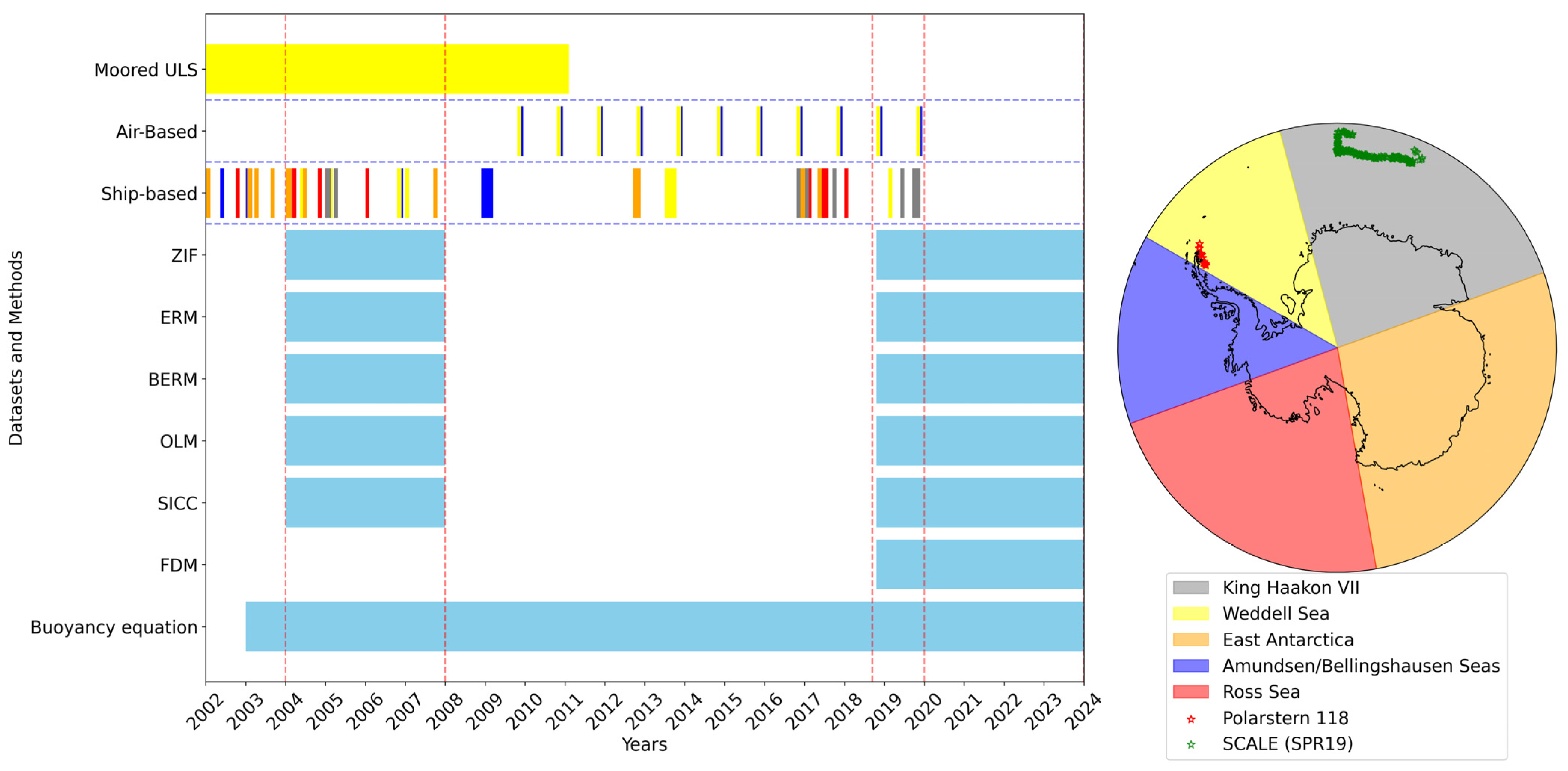
2.2. Field Observations

We analyzed the available public repositories for field observations of SIT (Table 1) to find the optimal time window to compare with the altimeter-derived SIT. They comprised SIT observations from drilled core lengths and ship-based visual estimations made by human observers following the ASPeCt protocol for Antarctic Sea-ice conditions. Our choice of data was informed by their spatio-temporal coverage during periods covered by satellites (Figure 1). The only considerable overlaps between field observations and satellites occur in the Weddell Sea and King Haakon VII region in 2019, and in the Weddell Sea between 2004 and 2008, a period that was previously studied by [3].

Hence, we selected the field data from the Southern oCean seAsonaL Experiment (SCALE) spring expedition and the summer Polarstern 118 expedition for assessment (see details and references listed in Table 1). Both the Polarstern 118 expedition and the SCALE spring expedition data were collected according to the ASPeCt protocol for making field observations in the Antarctic [26,43]. Additionally, the SCALE expedition data include drilled core measurements collected using the Kovacs Mark II coring system, made up of a barrel and an electric drill [43]. The thickness of the core was inferred from the length of the barrel and a ruler.

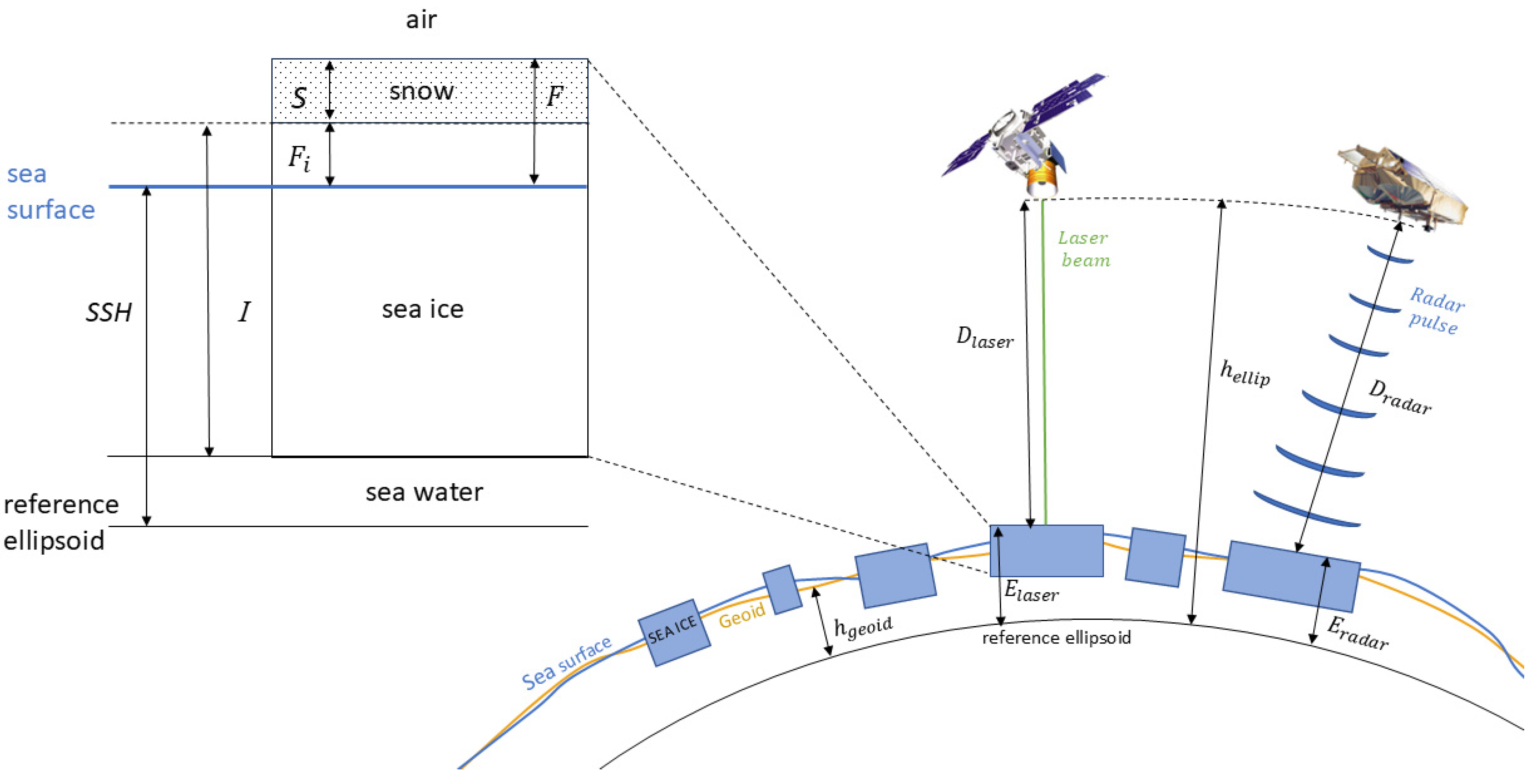
2.3. Estimation of SIT with Satellite Altimetry

Altimeters measure the elevation of the surface their signals are reflected from, which can be used to compute the SIT $\left(I\right)$. Lidar signals are reflected from the air–snow interface, and are used to obtain an estimate of the height of the combined snow and ice layer, $F$, while radar altimeters are assumed to return from the ice-snow interface, and are used to obtain a measure of the height of the ice layer only, $F_i$, because radar waves penetrate the snow layer [44].

Assuming isostatic balance of the ice floes in the water and applying the Archimedes’ principle, $I$ can be estimated from lidar freeboard retrievals using the buoyancy equation from [45]:

$$I=\left({\displaystyle \frac{{\rho }_w}{{\rho }_w-{\rho }_i}}\right)F+\left({\displaystyle \frac{{\rho }_s-{\rho }_w}{{\rho }_w-{\rho }_i}}\right)S$$

(1)

where $F$ is the freeboard height of the combined snow and ice layers above the sea surface, and $S$ is the snow depth (see Figure 2). ${\rho }_w$, ${\rho }_s$, and ${\rho }_i$ are the water, snow, and ice densities, each assigned the constant values $1023.9 \mathrm{k}\mathrm{g}/{\mathrm{m}}^3$, $300 \mathrm{k}\mathrm{g}/{\mathrm{m}}^3$, and $915.1 \mathrm{k}\mathrm{g}/{\mathrm{m}}^3$, respectively, as used in [9]. Note that we used these values throughout this paper.

All the published methods described in Section 2.3.1, Section 2.3.2, Section 2.3.3, Section 2.3.4, Section 2.3.5 and Section 2.3.6 and summarized in

Table 2. Methods used to derive Antarctic sea-ice thickness available in the literature. From the left, column one lists the full names and acronyms assigned to the methods in this paper, followed by their summary equation and the names used in the original publication as well as their reference. The description of symbols and the full equations for each method are available in Section 2.3.1, Section 2.3.2, Section 2.3.3, Section 2.3.4, Section 2.3.5 and Section 2.3.6 of the text.

Methods	Equations	Literature Names
Sea-Ice Climate Change Initiative (SICC)	$\mathrm{If} F>S: I=\left({\displaystyle \frac{{\rho }_w}{{\rho }_w-{\rho }_i}}\right)F+\left({\displaystyle \frac{{\rho }_s-{\rho }_w}{{\rho }_w-{\rho }_i}}\right)S$ If $F\le S: I=\left({\displaystyle \frac{{\rho }_s}{{\rho }_w-{\rho }_i}}\right)F$	SICC [3]
One-layer method (OLM)	$I=F{\displaystyle \frac{{\rho }_w}{{\rho }_w-{\rho }_i^{\ast }}}\ast {\displaystyle \frac{R}{R+1}}$	Improved One-Layer method [9]
Zero sea-ice freeboard method (ZIF)	$I=F\left({\displaystyle \frac{{\rho }_s}{{\rho }_w-{\rho }_i}}\right)$	ZeroIF [31]
Buoyancy equation and empirical relationship (BERM)	$I=\left({\displaystyle \frac{{\rho }_w}{{\rho }_w-{\rho }_i}}\right)F+\left({\displaystyle \frac{{\rho }_s-{\rho }_w}{{\rho }_w-{\rho }_i}}\right)(c+dF)$	Improved buoyancy equation [31]
Empirical relationship method (ERM)	$I=(a+bF)$	XOC in [32], originally developed by Xie et al. [33] and Ozsoy-Cicek et al. [34]
Freeboard differencing method (FDM)	$I=\left({\displaystyle \frac{{\rho }_w}{{\rho }_w-{\rho }_i}}\right)F+{\displaystyle \frac{1}{\eta }}\left({\displaystyle \frac{{\rho }_s-{\rho }_w}{{\rho }_w-{\rho }_i}}\right)(F-(F_i-\mathsf{\delta }\left)\right)$	Kwok et al. [35]

are variations of the buoyancy equation (Equation (1)), mostly differing for the parameterization of snow depth, and they all assume a layered geometry of the sea-ice–snow system as shown in Figure 2. To limit differences in the method estimations due to different spatio-temporal resolutions of the input satellite data, we first ensured that the input satellite data have the same spatio-temporal resolution as the already gridded IS-2 product (i.e., daily 25 km grid) by gridding daily along-track data from CS-2 onto the same IS-2 grid using a drop-in-bucket approach and by re-gridding the daily 12.5 km AMSR-E/AMSR2 product to the 25 km NSIDC polar stereographic grid.

We then computed the thickness at each grid cell from the six methods. Similarly, we computed the SIT uncertainty by applying the Gaussian error propagation at each grid cell, where ${\sigma }_{{\rho }_w}$, ${\sigma }_{{\rho }_s}$, and ${\sigma }_{{\rho }_i}$ are the uncertainties of the density of water, snow, and sea-ice, each assigned the constant values $3 \mathrm{k}\mathrm{g}/{\mathrm{m}}^3$, $100 \mathrm{k}\mathrm{g}/{\mathrm{m}}^3$, and $15 \mathrm{k}\mathrm{g}/{\mathrm{m}}^3$, respectively, as used in [9]. Note that we used these values throughout this paper. For uncertainty of the freeboard, we used the grid-wise standard deviation of the freeboard values within a grid cell as an estimate of the natural sea-ice freeboard uncertainty as performed in [46]. The estimate of snow depth uncertainty is needed for the SICC method (Section 2.3.5). Field-related values are not directly available from the released product [3,42] proposed to apply a constant relative error of 30% to the estimated thickness, which is a conservative value that we have also applied in our calculations.

We calculated the uncertainty of the SIT spatial mean as:

$$〈{\sigma }_I〉={\displaystyle \frac{\sum {\sigma }_I}{N}}$$

(2)

where $\sum {\sigma }_I$ is the sum of the SIT uncertainty of all grid cells, and N is the total number of grid cells with a valid SIT estimate.

We then computed the seasonal composites of the SIT estimates from each method for austral summer, autumn, winter, and spring, taken as December-to-February, March-to-May, June-to-August, and September-to-November, respectively. This was performed to increase the number of freeboard retrievals for each method.

2.3.1. The Zero Sea-Ice Freeboard (ZIF) Method

SIT estimation with the ZIF method [31] is based on the observation of sea-ice freeboard close to zero and even a few centimeters below the sea surface, as observed in the pack ice of the Ross and Amundsen/Bellingshausen Seas during the winter–spring transition period [47,48]. We refer to this method as lidar-only to differentiate it from the other lidar-based methods below that include other assumptions. When the sea-ice freeboard is close to zero, it can be assumed that the lidar-measured total freeboard is equal to the snow depth (i.e., $F=S$), and Equation (1) reduces to:

$$I=F\left({\displaystyle \frac{{\rho }_s}{{\rho }_w-{\rho }_i}}\right)$$

(3)

We estimated the SIT uncertainty, ${\sigma }_I$, according to Gaussian error propagation as (see also Supplementary Materials, Supporting Information S1):

$${\sigma }_I^2={\sigma }_{{\rho }_w}^2{\left({\displaystyle \frac{\partial I}{\partial {\rho }_w}}\right)}^2+{\sigma }_{{\rho }_i}^2{\left({\displaystyle \frac{\partial I}{\partial {\rho }_i}}\right)}^2+{\sigma }_{{\rho }_s}^2{\left({\displaystyle \frac{\partial I}{\partial {\rho }_s}}\right)}^2+{\sigma }_F^2{\left({\displaystyle \frac{\partial I}{\partial F}}\right)}^2$$

(4)

where ${\sigma }_F$ is the uncertainty of the total freeboard estimated from the standard deviation of the total freeboard within each grid cell as explained in the previous section.

2.3.2. The Empirical Relationship Method (ERM)

Using in situ drill measurements of SIT, sea-ice freeboard, and snow depth, from 15 cruises that provide a combined coverage of the circumpolar region during autumn (February/March), mid to late winter (June to September), and late winter/spring (September to November), [33,34] proposed a set of regional empirical relationships between total sea-ice freeboard, SIT, and snow depth as follows:

$$I=(a+bF)$$

(5)

$$S=(c+dF)$$

(6)

where the coefficients $a$, b, c, and d are different for the Antarctic regional sectors (Figure S1, and Table S1). The longitudinal extent of the sectors in degrees East are: Indian Ocean (20–90°), Pacific Ocean (90–160°), Eastern Weddell Sea (315–320°), Western Weddell Sea (300–315°), Bellingshausen/Amundsen Sea (230–300°), and Ross Sea (160–230°).

We estimated the SIT uncertainty ${\sigma }_I$ according to Gaussian error propagation as (see also Supplementary Materials, Supporting Information S1):

$${\sigma }_I^2={\sigma }_F^2{\left({\displaystyle \frac{\partial I}{\partial F}}\right)}^2+{\sigma }_a^2{\left({\displaystyle \frac{\partial I}{\partial a}}\right)}^2+{\sigma }_b^2{\left({\displaystyle \frac{\partial I}{\partial b}}\right)}^2$$

(7)

where ${\sigma }_a=0.1 \mathrm{m}$ and ${\sigma }_b=0.3\ast b$ are the uncertainties of the empirical parameters $a$ and b, respectively [9,37]. ${\sigma }_F$ is the uncertainty of the total sea-ice freeboard as used in the previous methods.

2.3.3. Combined Buoyancy Equation and Empirical Relationship Method (BERM)

This method was also proposed by [31]; it replaces the snow depth $S$ in Equation (1) with the empirical formula in Equation (6). The buoyancy Equation (1) is modified as follows:

$$I=\left({\displaystyle \frac{{\rho }_w}{{\rho }_w-{\rho }_i}}\right)F+\left({\displaystyle \frac{{\rho }_s-{\rho }_w}{{\rho }_w-{\rho }_i}}\right)(c+dF)$$

(8)

Similarly, we computed the SIT uncertainty according to the Gaussian error propagation as (see also Supplementary Materials, Supporting Information S1):

$${\sigma }_I^2={\sigma }_{{\rho }_w}^2{\left({\displaystyle \frac{\partial I}{\partial {\rho }_w}}\right)}^2+{\sigma }_{{\rho }_i}^2{\left({\displaystyle \frac{\partial I}{\partial {\rho }_i}}\right)}^2+{\sigma }_{{\rho }_s}^2{\left({\displaystyle \frac{\partial I}{\partial {\rho }_s}}\right)}^2+{\sigma }_F^2{\left({\displaystyle \frac{\partial I}{\partial F}}\right)}^2+{\sigma }_c^2{\left({\displaystyle \frac{\partial I}{\partial c}}\right)}^2+{\sigma }_d^2{\left({\displaystyle \frac{\partial I}{\partial d}}\right)}^2$$

(9)

2.3.4. The One-Layer Method (OLM)

SIT estimation with the OLM [9] is calculated by treating the sea-ice–snow system as a single layer with a reduced density (Figure 2, Equation (1)), and assuming isostatic balance of the ice floes in the water. Equation (1) becomes:

$$I=F{\displaystyle \frac{{\rho }_w}{{\rho }_w-{\rho }_i^{\ast }}}\ast {\displaystyle \frac{R}{R+1}}$$

(10)

where ${\rho }_i^{\ast }$ is the reduced density of the combined ice-snow layers and is equal to ${\displaystyle \frac{R\ast {\rho }_i+{\rho }_s}{R+1}}$. $R$ is the ratio of the parameterized SIT to the snow depth from the empirical relationships in Equations (5) and (6).

We computed the uncertainty of SIT according to the Gaussian error propagation (see also Supplementary Materials, Supporting Information S1):

$${\sigma }_I^2={\sigma }_{{\rho }_w}^2{\left({\displaystyle \frac{\partial I}{\partial {\rho }_w}}\right)}^2+{\sigma }_{{\rho }_i}^2{\left({\displaystyle \frac{\partial I}{\partial {\rho }_i}}\right)}^2+{\sigma }_{{\rho }_s}^2{\left({\displaystyle \frac{\partial I}{\partial {\rho }_s}}\right)}^2+{\sigma }_F^2{\left({\displaystyle \frac{\partial I}{\partial F}}\right)}^2+{\sigma }_a^2{\left({\displaystyle \frac{\partial I}{\partial a}}\right)}^2+{\sigma }_b^2{\left({\displaystyle \frac{\partial I}{\partial b}}\right)}^2{\sigma }_c^2{\left({\displaystyle \frac{\partial I}{\partial c}}\right)}^2+{\sigma }_d^2{\left({\displaystyle \frac{\partial I}{\partial d}}\right)}^2$$

(11)

where all the symbols have been introduced in the previous methods.

Note that the proposed OLM is hypothesized to be optimal when applied to point-specific information to calculate dynamic $R$ values for each sensor data point [32]. In this paper, we applied the method at the scale of the IS-2 data (i.e., daily 25 km grid) for purposes of intercomparing with the other methods and to derive an estimate of the uncertainty within the grid cell.

2.3.5. The Sea-Ice Climate Change Initiative Method (SICC)

The SICC approach uses a combination of the buoyancy equation (Equation (1)) and the assumption of zero-ice freeboard (Equation (2)) by distinguishing between cases where the sea-ice freeboard is positive and where it is negative [3]. This is calculated by comparing the magnitude of the lidar-derived sea-ice freeboard with that of the snow depth from passive microwave data. Sea-ice freeboard is then considered to be positive where it is greater than the snow-thickness and negative where it is less than or equal to the snow depth. SIT is then estimated as:

$$F>S: I=\left({\displaystyle \frac{{\rho }_w}{{\rho }_w-{\rho }_i}}\right)F+\left({\displaystyle \frac{{\rho }_s-{\rho }_w}{{\rho }_w-{\rho }_i}}\right)S$$

(12)

$$F\le S: I=\left({\displaystyle \frac{{\rho }_w}{{\rho }_w-{\rho }_i}}\right)F$$

(13)

In our analysis, F is the total freeboard from IS-2 and $S$ is the snow depth from the AMSR-E/AMSR-2 gridded snow depth product (Section 2.1).

The SIT uncertainty for Equations (12) and (13) are computed according to the Gaussian error propagation (see also Supplementary Materials, Supporting Information S1):

$$F>S: {\sigma }_I^2={\sigma }_{{\rho }_w}^2{\left({\displaystyle \frac{\partial I}{\partial {\rho }_w}}\right)}^2+{\sigma }_{{\rho }_i}^2{\left({\displaystyle \frac{\partial I}{\partial {\rho }_i}}\right)}^2+{\sigma }_{{\rho }_s}^2{\left({\displaystyle \frac{\partial I}{\partial {\rho }_s}}\right)}^2+{\sigma }_F^2{\left({\displaystyle \frac{\partial I}{\partial F}}\right)}^2+{\sigma }_S^2{\left({\displaystyle \frac{\partial I}{\partial S}}\right)}^2$$

(14)

$$F\le S: {\sigma }_I^2={\sigma }_{{\rho }_w}^2{\left({\displaystyle \frac{\partial I}{\partial {\rho }_w}}\right)}^2+{\sigma }_{{\rho }_i}^2{\left({\displaystyle \frac{\partial I}{\partial {\rho }_i}}\right)}^2+{\sigma }_{{\rho }_s}^2{\left({\displaystyle \frac{\partial I}{\partial {\rho }_s}}\right)}^2+{\sigma }_F^2{\left({\displaystyle \frac{\partial I}{\partial F}}\right)}^2$$

(15)

As explained in Section 2.3, we used ${\sigma }_s=0.3\ast S$ as proposed by [3].

2.3.6. The Freeboard Differencing Method (FDM)

Ref. [35] proposed a method to take advantage of the concurrent availability of lidar and radar altimetry since 2019. The snow depth $S$ is computed by subtracting the CS-2 sea-ice freeboard ($F_i$) from the IS-2 total freeboard ($F$) and accounting for deviations in radar path length because of the refractive index of the snow layer. SIT is then estimated with a modified buoyancy equation:

$$I=\left({\displaystyle \frac{{\rho }_w}{{\rho }_w-{\rho }_i}}\right)F+{\displaystyle \frac{1}{\eta }}\left({\displaystyle \frac{{\rho }_s-{\rho }_w}{{\rho }_w-{\rho }_i}}\right)(F-F_i)$$

(16)

where $\eta$ is the refractive index at Ku-band (CS-2 altimeter’s wavelength range).

The implementation used in this paper also follows the approach proposed by [38], wherein daily along-track IS-2 and CS-2 freeboards (weighted by AMSR-E/AMSR2 SIC) are first averaged separately onto their own $25 \mathrm{k}\mathrm{m}$ grids at daily temporal resolution, then the two freeboards are differenced at each IS-2 grid cell using CS-2 freeboards that are within a $75 \mathrm{k}\mathrm{m}$ box, with time separations $|∆T|<10 \mathrm{d}\mathrm{a}\mathrm{y}\mathrm{s}$ to the IS-2 grid cells to provide a better spatial coverage.

We propagated the error as (see also Supplementary Materials, Supporting Information S1):

$${\sigma }_I^2={\sigma }_{{\rho }_w}^2{\left({\displaystyle \frac{\partial I}{\partial {\rho }_w}}\right)}^2+{\sigma }_{{\rho }_i}^2{\left({\displaystyle \frac{\partial I}{\partial {\rho }_i}}\right)}^2+{\sigma }_{{\rho }_s}^2{\left({\displaystyle \frac{\partial I}{\partial {\rho }_s}}\right)}^2+{\sigma }_F^2{\left({\displaystyle \frac{\partial I}{\partial F}}\right)}^2+{\sigma }_{F_i}^2{\left({\displaystyle \frac{\partial I}{\partial F_i}}\right)}^2$$

(17)

where ${\sigma }_F$ and ${\sigma }_{F_i}$ are the standard deviations of the total freeboard and the ice freeboard at the grid cell scale, respectively.

Ref. [38] identified a potential bias in CS-2 freeboards, leading to an overestimation of ice thickness. This bias is attributed to the radar partially penetrating the snow layer and reflecting from a point above the true ice–snow interface. In particular, the four sectors, characterized by predominantly seasonal ice (i.e., Ross, King Haakon, and East Antarctic), exhibit the lowest sector-averaged CS-2 freeboards with low seasonal variability. Based on these observations, we applied a 6 cm adjustment to the freeboard measurements in this study to provide a better estimate of ice thickness as in [38]. Although current knowledge does not permit adjustments to individual thickness retrievals, Ref. [38] notes that these large-scale adjustments likely provide a better estimate than those calculated solely using freeboard differences, offering a more reliable representation of the ice conditions. To do this, we adjusted CS-2 freeboards by modifying Equation (16) to:

$$I=\left({\displaystyle \frac{{\rho }_w}{{\rho }_w-{\rho }_i}}\right)F+{\displaystyle \frac{1}{\eta }}\left({\displaystyle \frac{{\rho }_s-{\rho }_w}{{\rho }_w-{\rho }_i}}\right)(F-(F_i-\delta \left)\right)$$

(18)

2.4. Comparison with Field Observations

We compared the satellite-derived SIT with the field observations selected in Section 2.2. Due to the limited spatial representativeness of the field estimations, a direct comparison is not meaningful; therefore, we compared monthly statistics of the field estimations and the satellite-derived SIT. We first sliced the altimeter-derived SIT to the time and space covered by the field observations and found the data nearest to the available field observation within a 1 km radius and a time separation of not more than 15 days. We then compared the distribution of the nearest field observations with the altimeter-derived SIT distribution from each method and calculated the Wasserstein Distance (WD) to quantify the discrepancy.

WD, also known as the Earth-mover’s distance, is a measure of the dissimilarity between two distributions through an estimation of the work that would be needed to transform one distribution into another distribution with the same sample size such that equivalent distributions have a WD of 0 [49].

WD is sensitive to geometric dissimilarities between two distributions, making it a useful metric to quantitatively measure dissimilarities [50]. Ref. [51] demonstrated the usefulness of the WD-based metric to complement the existing methods used for intercomparing climate models, such as ranking their performance by the root mean square error of the median of an ensemble. We refer the reader to this publication for a dedicated usage of the metric in intercomparison studies. Similarly, we use the WD-based metric to assess the dissimilarity of the SIT distributions estimated from the satellite methods to the same field dataset to complement our visual comparison of the distributions. In this paper, we use the python package SciPy version 1.10.0 to calculate the WD.

3. Results

This section first presents the comparison with the field observations selected in Section 2.2, and it is followed by a spatial intercomparison of the six methods described in Section 2.3 for the reference year 2019, aimed at understanding their similarities and features, and lastly by an analysis of their spatial mean timeseries over the period of overlap in 2019–2023 (Figure 1).

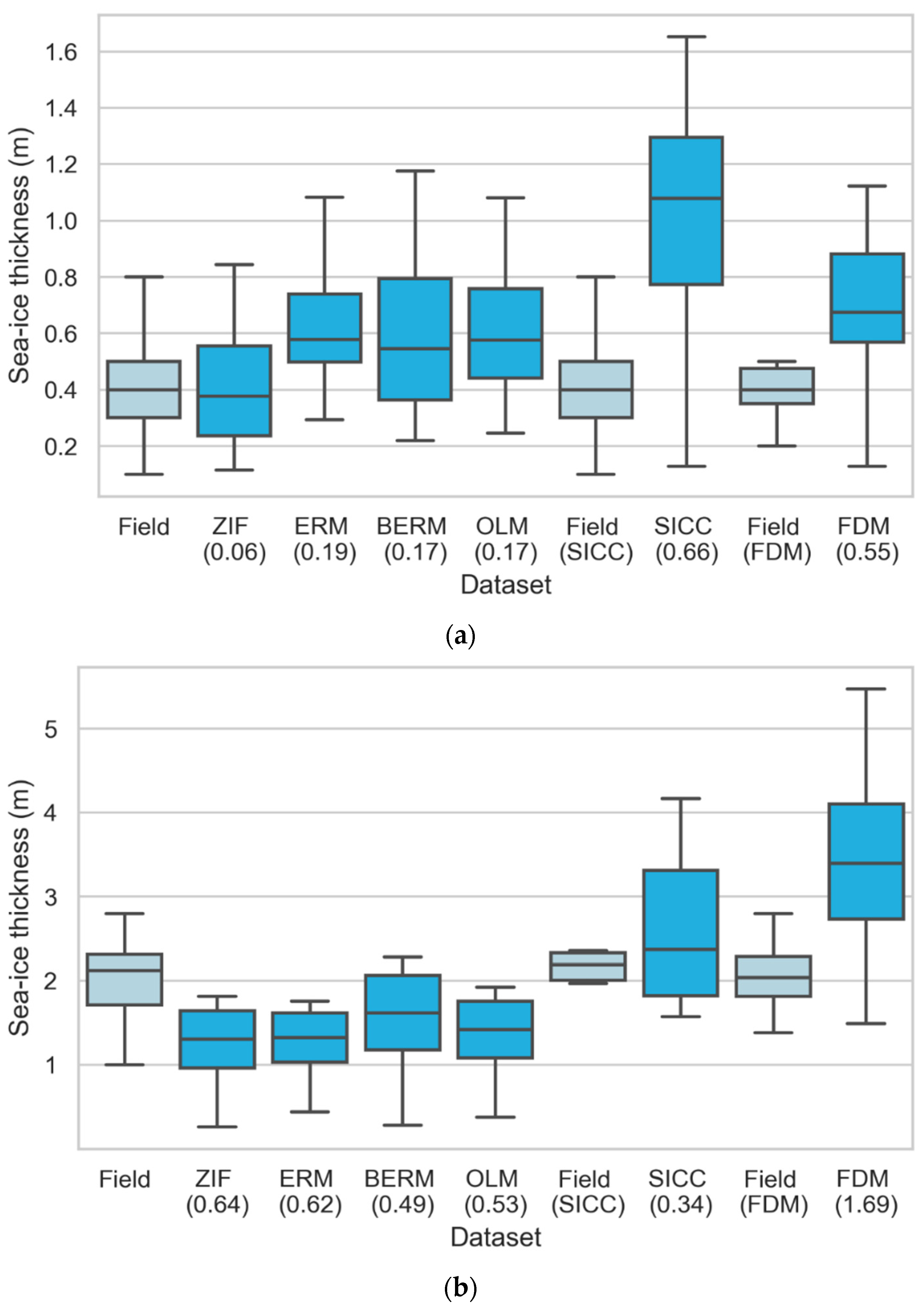
3.1. Assessment with Field Observations

Figure 3a shows the comparison of the co-located distributions in the marginal ice zone of the King Haakon VII Sea sector in the spring of 2019 from the SCALE cruise (Table 1). The individual distributions are shown in Figure S2 in the Supplementary Material. In this region and season, sea-ice was thin, with a median of 0.4 m and an interquartile range between 0.3 and 0.5 m. The ZIF method matches the field observations better than the other methods with the lowest WD value, demonstrating its robustness in capturing low freeboard ice conditions. This supports the observations of [3], who noted ZIF’s reliability under similar conditions. The method’s ability to capture these low-freeboard conditions can be attributed to its assumption that sea-ice freeboard is close to zero, which is common in areas with thin, seasonal ice [47,48]. The BERM and OLM methods also perform well, showing slightly higher WD values yet keeping a strong alignment with the observed data. These similarities could come from the shared usage of the empirical linear relationship between the total freeboard and snow depth (i.e., Equation (6)).

In contrast to the comparison in the King Haakon VII Sea sector during spring, the analysis of thicker, multi-year ice in the Weddell Sea during summer shows a different picture. Here, the ZIF method substantially underestimates SIT, evident from its significantly higher WD value compared to other lidar-based methods. This agrees with the findings of [3,52], who noted that ZIF’s assumption of zero freeboard likely leads to underestimations in areas where sea-ice is thicker and freeboard values exceed zero. Similarly, the other lidar-based methods also underestimate the thickness of the ice in this region and period. This is likely due to a mismatch of the linear relationship between the snow depth and freeboard, since all of them use the empirical relationship method. Furthermore, it has been observed by [52] in the Amundsen/Bellingshausen Seas and Weddell seas in October of 2010 and 2011 using airborne measurements that the snow depth was only linearly related to the freeboard when the freeboards were low. We noted that OLM and BERM evidently perform better than the other lidar-based methods, indicated by their lower WD and better overlap with field data.

Notably, SICC performs most effectively in the Weddell Sea in terms of the median, showing the lowest WD value under thicker, multi-year ice conditions. The difference in dispersion could be due to the limits of the data that did not sample the field variance entirely. This contrasts with its performance in the King Haakon VII sector’s thin ice, suggesting that SICC’s snow depth treatment and multi-sensor approach improves its accuracy in regions with thicker ice. The FDM overestimates SIT in both the thin and thick ice regimes considered in this study. FDM performed slightly better in the thin-ice region than in the thick-ice region, which may be due to CS-2 freeboards being biased in favor of deformed or flooded ice regions or that the adjustment to CS-2 freeboards is more impactful in this sector; [38] notes that the impact is larger in sectors covered with thinner ice.

These provisional comparisons with spatially extended observations show the need to select satellite-based SIT estimation methods that are regionally and seasonally appropriate, as they highlight the significant influence of snow depth and the need to carefully consider the underlying assumptions when using these methods. However, the selected available data are insufficient to give an overall assessment of the skills of each method and to rank them. It is therefore of interest to evaluate through the intercomparison exercise presented in the next section if the methods share common features or peculiar differences that are observed at larger scales in specific regions or periods.

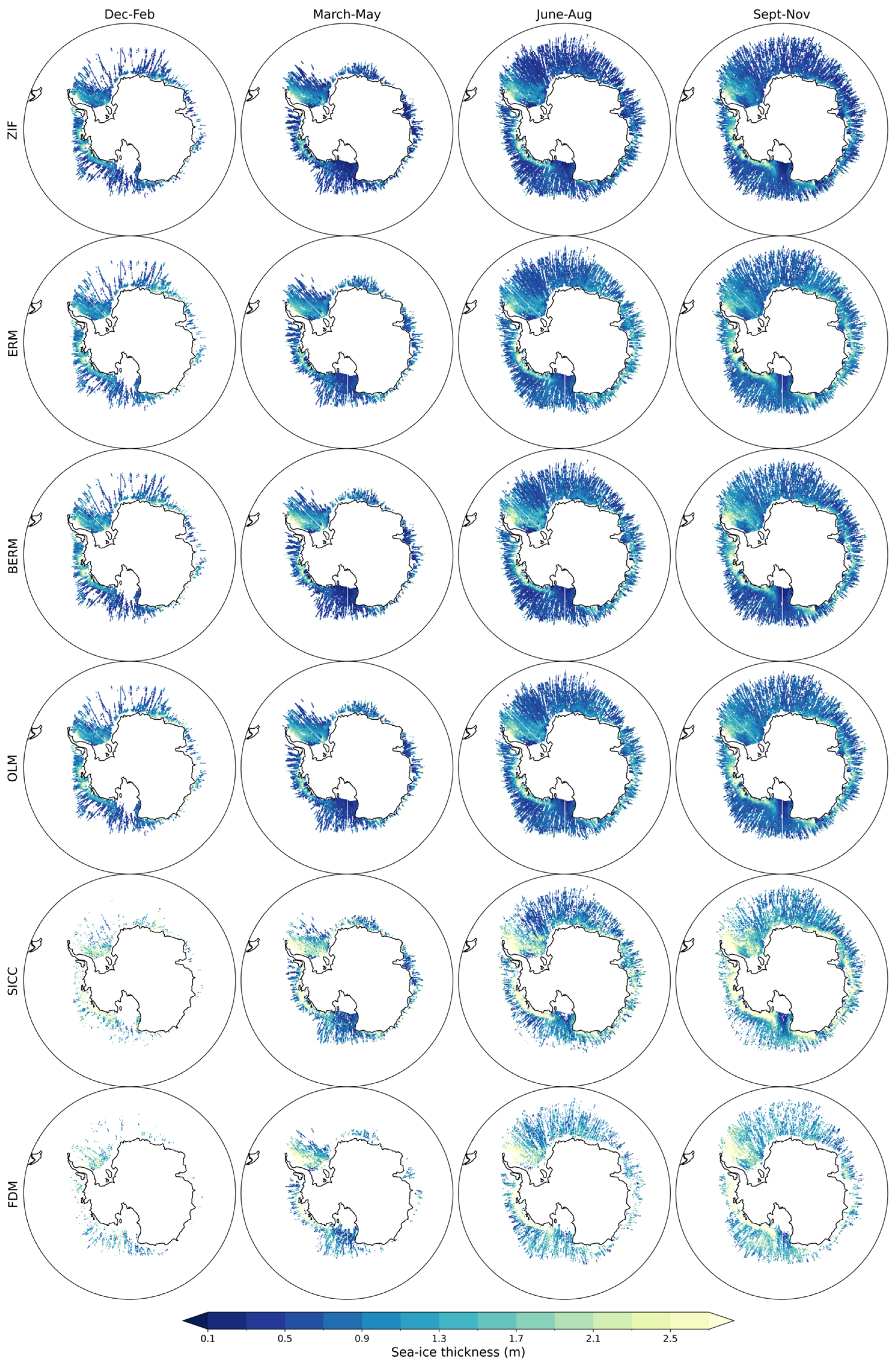
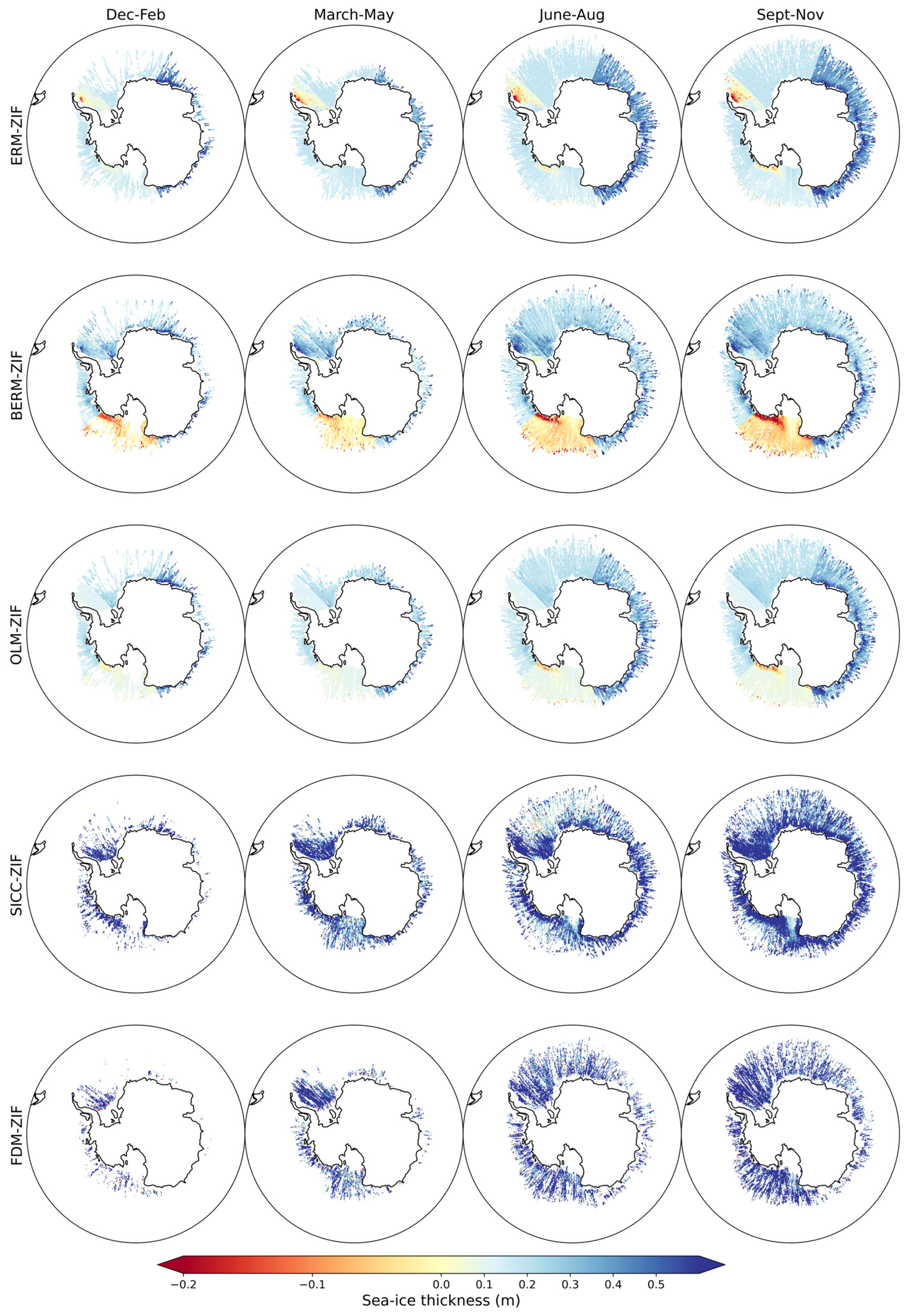
3.2. Spatial Intercomparison of Satellite Methods

The seasonal composites of SIT for the reference year 2019 show similar patterns and features among the six methods, with some exceptions (Figure 4). The ERM, BERM, and OLM methods are visually more similar to one other and have the same coverage because they are variations of the same methodology. SICC and FDM differ in overall magnitude with respect to the others, and FDM is also characterized by a smaller number of observations due to the need for two sets of concurrent altimeter data. All methods produce known features of Antarctic Sea-ice, such as the arrangement of thicker ice around the coast and a general thinning towards the ice margins. This arrangement is most noticeable from June to November in the ZIF, ERM, BERM, OLM, and SICC methods. Although not strong, this arrangement does persist through summer and autumn; however, it is not as clear due to the reduced extent of the ice. The FDM shows this arrangement most clearly in the Amundsen/Bellingshausen Sea and the East Antarctic sectors between June and November. All the methods show that the presence of the Ross Sea polynya is most noticeable from March to November. As noted by [3,38] when describing their methods, polynyas appear as ice thinner than observed along the rest of the coastline and in the Ross Sea sector. All methods also show an area of thicker ice in the western Weddell Sea in all periods, an area known to be covered by multi-year ice [3].

3.2.1. Marginal Ice Zone Features

We note that in Figure 4, all the methods, independently of the different combinations of sensors and algorithms, show anomalously thick ice in the marginal ice zone (MIZ) where one would anticipate thinner ice. These values are most noticeable when one zooms in on the ice edge of the East Antarctic sector between June and November across all the methods, but they are present in all the other sectors and periods to varying extents. These may be caused by erroneous freeboard retrievals from IS-2 near the ice edge. The gridded sea-ice freeboards from IS-2 released as the ATL20 product are generated from the along-track sea-ice freeboard product (ATL10), in which the freeboards have been calculated from sea-ice height segments and reference sea surface height segments computed in ATL07 [53]. In ATL07, erroneous retrieval of sea surface heights occurs due to depression of the sea surface to tens of centimeters below the local mean sea level during the penetration of waves into the ice cover, resulting in erroneously high freeboard samples near the ice edge [53]. IS-2 can in fact be used to retrieve waves in ice in the marginal ice zone [54]. These erroneously higher freeboards would result in higher-than-expected SIT estimates near the ice edge, which are assumed to be mostly removed by filtering out all height segments in regions with less than 50% sea-ice concentration [55]. Ref. [3] reported similar higher-than-expected thick estimates along the ice edge from IS-2 predecessor satellite ICESat-1. Our results indicate that concentration filtering in IS-2 is insufficient and may impact all regions with MIZ features, which have been reported to extend further poleward than previously thought in the Southern Ocean [56]. This is a known issue, and an improved filtering strategy is being tested by the product developers [55].

3.2.2. Spatial Patterns

Based on the similarity between the first four methods and considering that the ZIF method is the simplest approach, we used it as reference to spatially compare against the other methods (Figure 5). We find that all the methods generally give thicker ice with respect to ZIF. There is no discernable spatial pattern of differences with the FDM due to sparse spatial coverage. A pattern emerges with the SICC, in which the methods have the largest differences in the regions predominantly covered with thick ice, namely around the coast and in the Weddell Sea. The lowest differences occur in regions predominately covered with thin ice. The differences are lower in regions of thin ice because the SICC likely switches to the assumption of zero-ice freeboard in these regions, matching the ZIF method. However, this does not apply to entire sectors since we saw considerable differences in the sector-based distributions of the two methods (Figure 6), even in sectors with the lowest median thicknesses such as in the Ross Sea sector and the Kind Haakon VII Sector as further discussed in the next section.

The 3 lidar methods ERM, BERM, and OLM that use the empirical Equations (5) and (6) show sector-wise differences with the ZIF estimations. They are generally thicker than ZIF in all the sectors except in the Ross Sea sector for all the methods and in the western Weddell Sea sector for the ERM. They also present distinct thickness offsets for adjacent sectors that are in the range of the mean circumpolar thickness obtained by these methods (see Figure 6 and Figure 7). These sector-wise differences are the result of differences between the empirical coefficients used for each sector. We see that when only Equation (5) is used, such as in ERM, one acquires differences across four sectors, which correspond to the differences between coefficients of adjacent sectors (i.e., a and b coefficients), while we acquire three discontinuities when using Equation (6) only (BERM), because the c and d coefficients are different for three sectors. We then see that when both Equations (5) and (6) are used, such as in OLM, we receive five sector-based differences due to the combination of all the coefficients. In the case of BERM, the empirical Equation (6) leads to a negative offset in the Ross Sea sector of more than 0.2 m, and the same happens in the Antarctic Peninsula for ERM. We noticed that these methodological offsets are less of concern due to the thicker average ice in these sectors (cfr. Figure 6). The differences are also noticeable in the spatial maps of ERM, BERM, and OLM for all periods (Figure 4), in which we can respectively distinguish four, three, and five distinct thickness regimes coinciding with the sectors used in the empirical equations during all periods in 2019. This implies that these methods should be used to compare thickness values within the same sector, because inter-sectoral comparisons will be aliased by the choice of the coefficient values, which are based on limited sets of observations from each sector. Furthermore, this implies that sectors should be defined following [33,34] when making sector-based comparisons using these methods. For this reason, we defined sectors following Figure S1 in Section 3.3 and Section 3.4.

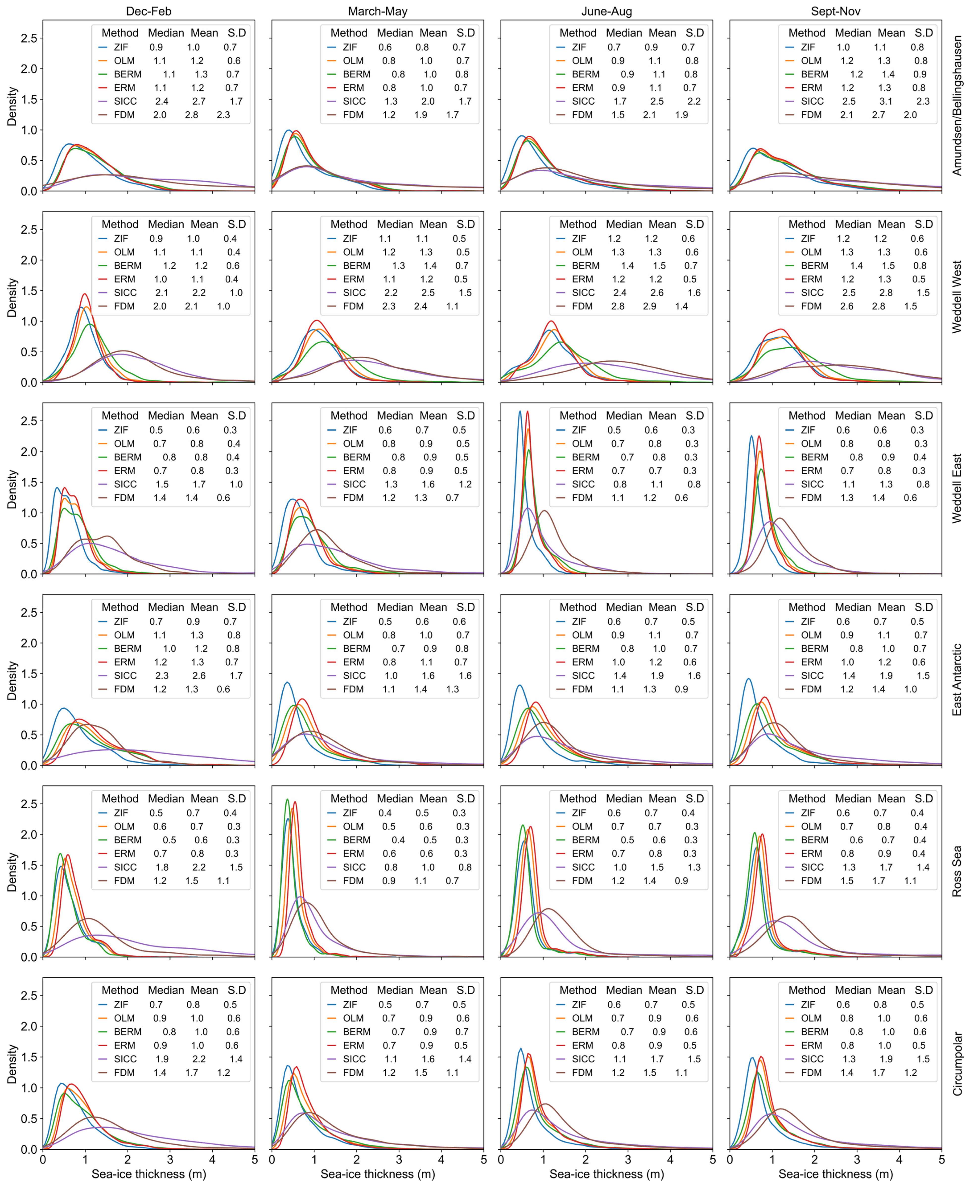
3.3. Thickness Distribution Intercomparison

The main features of each method can be further appreciated by looking at the regional and circumpolar distributions of the thickness (Figure 6). All methods present mostly unimodal distributions skewed towards thicker ice throughout the year, except in the Weddell West, in which the distributions are less skewed, aligning with the results previously reported in the literature using a subset of the methods presented here [3,9,38]. Confirming the visual interpretation of Figure 4, the ERM, BERM, and OLM methods are most alike in terms of their mean thicknesses, the range of thickness covered, and the seasonal progression; similarly, SICC and FDM are more similar to each other. Overall, SICC and FDM estimate the thickest ice in all the periods and sectors, while ZIF estimates the thinnest ice as observed in Figure 3 and Figure 4.

The distributions with the thicker median values are mostly observed during spring in all the sectors across the methods. During this period, the thickest ice is observed in the Amundsen/Bellingshausen Seas and Weddell West sectors with medians of more than 2 m for the SICC and FDM and more than 1 m for the other methods. The SICC and FDM distributions are flat and have fat tails during this period in both sectors, as indicated by the large mean, median, and standard deviations. These sectors have been reported to have the thickest snow and ice [38,39]. Furthermore, ref. [38] remarked that the Amundsen/Bellingshausen sector had high snow depth in 2019; due to persistent onshore wind pattern that resulted in coastal convergence based on these observations, we expect that all the methods would be less similar in these sectors due to the greater role of the snow depth. This applies in winter and spring of the Amundsen/Bellingshausen and Weddell Sea sectors, in which we observe the largest differences between the mean and median values of the lidar-based methods and the SICC and FDM. However, we do not rule out that these pronounced differences may be a result of a different process than an impact of snow depth uncertainty.

The distributions with thinner median values are mostly observed during autumn in all methods and sectors, except in the Weddell Sea, in which the thinnest ice is observed during summer. This is due to the presence of multi-year ice in the Weddell West sector that substantially thins during the summer melt. In the other sectors, thinner seasonal ice mostly melts in summer, leaving behind only thicker ice, resulting in larger mean and median ice thickness values as observed in Figure 4. The strong deformation features that have been reported for the Ross Sea and Weddell Sea in winter and spring [57,58] are more likely to be local phenomena, since the distributions do not show any sign of skewness towards thicker ice in these sectors. We noticed the similarity between the Ross Sea distributions from SICC and FDM with the circumpolar distribution, while this was not observed in the Weddell East sector that also holds the largest extent of sea-ice.

There was no appreciable seasonal change of shape in the circumpolar distributions across the methods. We only noticed a seasonal change in the Weddell West distributions, wherein the distributions progressively became flatter from summer to spring, most noticeably in the FDM and SICC distributions. However, all the distributions do progressively broaden to cover slightly thicker ice from summer to spring across the sectors, indicating a slight seasonality of Antarctic ice.

Overall, these findings underscore that while each method has distinct regional and seasonal performance characteristics, the differences in thickness distributions reveal their specific sensitivities to snow depth and freeboard assumptions. Selecting the appropriate method based on regional ice conditions, especially in areas of substantial snow and ice convergence, remains critical for achieving accurate sea-ice thickness estimates. Additionally, comparisons with observations presented in Section 3.1 indicate that the SICC is more likely to perform well under thicker ice conditions, while the lidar-based methods have better skills with thinner ice. We thus propose to use the methods in a complementary way rather than contrasting their features. We will then assume that the two clusters observed in the distributions (i.e., lidar-based methods vs. SICC and FDM) are components of the same population, although with this approach it is not possible to distinguish the relative abundance of thicker and thinner sea-ice. We are also cognizant that any interpretation is only valid for this reference year, and it may be different in other years. The next Section 3.4 will give an initial overview of the interannual variability.

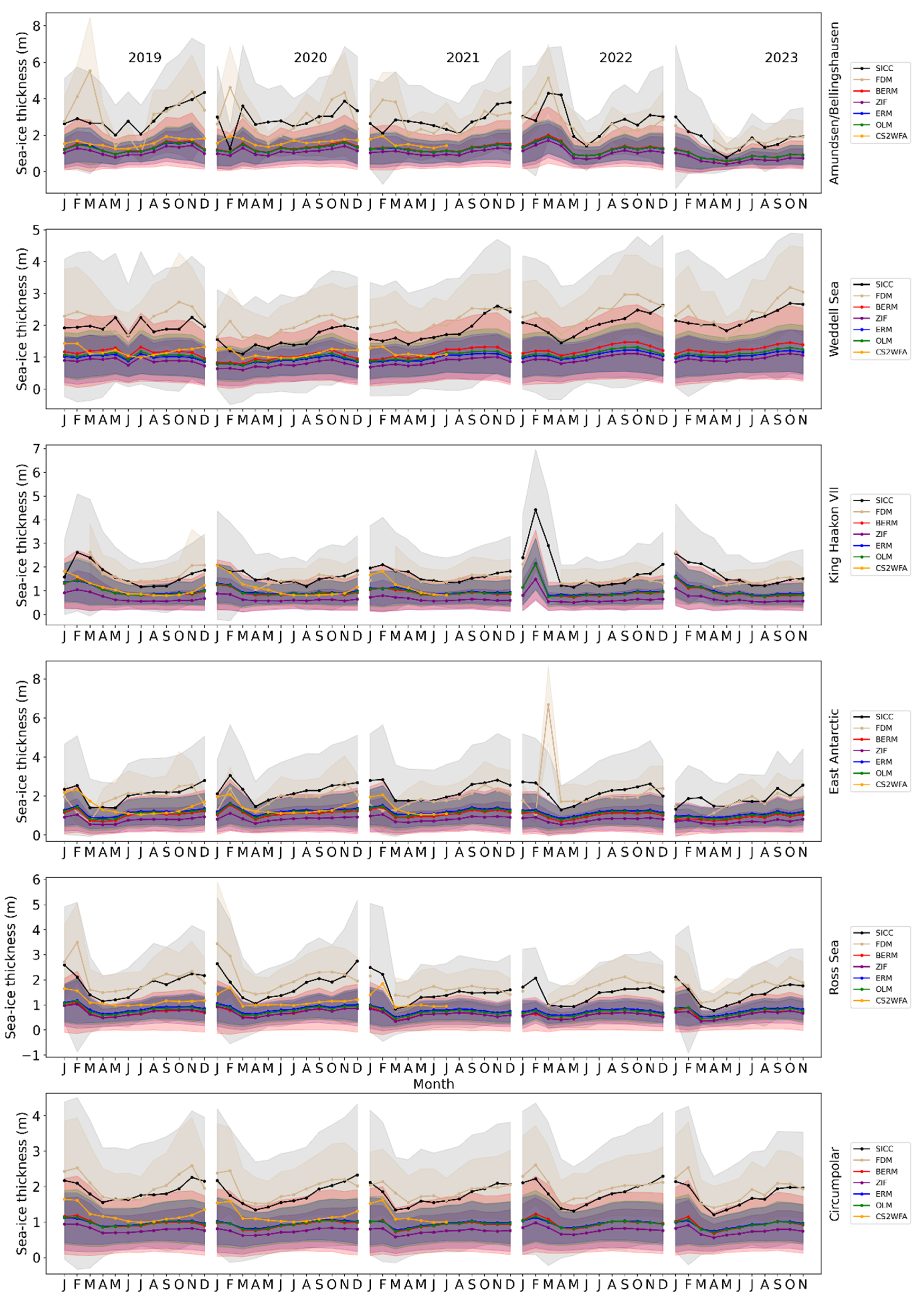
3.4. Interannual Variability over the Past 5 Years

The overlap period indicated in Figure 1 allows us to perform a preliminary intercomparison of the SIT time-series (Figure 7). The spatial SIT averages for each sector and month have been computed and plotted with the mean uncertainty as defined in Section 2. We also added the estimates from [39] for a comparison against an alternative independent method. We used the snow depth and ice freeboards derived with their CS-2 Waveform-Fitting method for Antarctic Sea-ice (CS2WFA hereon) to calculate the thicknesses from 2019 to July 2021. Note that these data are only published until this period.

Over the past 5 years covered in the time-series, at the circumpolar scale, the methods based on Equations (5) and (6) are mostly alike (i.e., ERM, BERM, and OLM), with estimates of a small seasonality in all sectors and ranges between 0.5 and 1 m. ZIF consistently estimates the thinnest ice, following the same seasonality as the former methods, while SICC and FDM alternatingly estimate the thickest ice, confirming the clustering observed in Section 3.3. The CS2WFA estimates fall between the two clusters of methods as noted by [39] but closely match the lidar-based methods between April and October of 2019 and 2020. Overall, the CS2WFA always falls within the uncertainty range of the lidar-based methods, while the SICC and FDM remain at the upper limit of those uncertainties except in the Ross Sea and Amundsen/Bellingshausen Sea sectors from 2019 to 2023 and 2019 to 2022, respectively.

Similarly, on the regional scale, SICC and FDM are remarkably similar. The lidar-based methods using Equations (5) and (6) are expected to be similar since they incorporate the same empirical equations as discussed in Section 3.2 and Section 3.3, but it is not clear how the SICC and FDM, which use different processing steps and assumptions, are so similar in estimated thickness values. The CS2WFA estimates only remain between the two clusters of methods in the Ross Sea and Amundsen/Bellingshausen Sea sectors from 2019 to 2021, while it closely matches the lidar-based methods in the other sectors between June and November of each year. It is difficult to say which set of methods (i.e., SICC and FDM or the lidar-based methods) are most reliable due to the consistently large uncertainties and the limited available field data to compare against.

Overall, at both the circumpolar and regional scale in all the years, the two sets of methods, the lidar-based methods (including the CS2WFA estimates) and the SICC and FDM have the largest differences in the mean thickness during the ice growth period between winter and spring. Whether this is indicative of the SICC and FDM simply growing too much ice, due to underestimating the snow depth, or a decay of the linear relationship between the ice freeboard and the snow depth cannot be ascertained without a detailed analysis of the contributing factors to Antarctic ice development and corresponding direct measurements in multiple sectors. We noted that the limited comparison made in Section 3.1 does not give further information about this due to its limited temporal range. However, considering that the CS2WFA estimates do not use the linear relationship between the freeboard and the snow depth, it is likely that the SICC and FDM underestimate the thickness of snow during this period, resulting in an overestimation of the ice thickness. Since snow depth is obtained in two different ways, from a satellite product in SICC and by differencing altimetry data in FDM, it is puzzling that there is such a similarity. Only the design of concerted calibration experiments with in situ data will allow us to determine the reasons.

Lastly, we noted that despite the discrepancies between all the methods, they all show a low seasonal and interannual variation in the mean ice thickness at both the regional and circumpolar scale, except for the SICC and FDM in most sectors. This may indeed be an overall large-scale characteristic of Antarctic Sea-ice, considering the consistently large uncertainties in each method, it appears at this stage premature to make interannual comparisons of the monthly mean ice thickness because any change is masked by the large uncertainties. We did, however, note a small negative trend across the methods in the Amundsen/Bellingshausen and Ross Sea sectors throughout the months, and a positive trend in the Weddell West sector, as can be visually confirmed with Figure S6, which shows the same time-series without uncertainty information to easily identify the small trends.

3.5. Potential Impact of Inaccurate Snow Depth and Freeboard Assumptions

For the lidar-only methods that apply the regional empirical relationships, potential biases may occur from the limits of ASPeCt observations used to estimate linear relationships. As mentioned in Section 1, the ASPeCt dataset is biased towards thin ice due to thick ice avoidance by ships, often missing deeper snow on deformed sea-ice and very thick sea-ice [59]. Furthermore, the ASPeCt dataset used to compute the relationships is not homogenous in space and time, covering the period between 1986 and 2007, mostly in August/September, missing the summer (melting) and winter (freezing) periods [34].

For SICC, inaccurate snow depth estimates from the AMSR-E/AMSR2 dataset impact the discrimination of negative from positive sea-ice freeboard, and the estimation of SIT where the freeboard is greater than the snow depth. Growth and melting of the snow layer will affect the observed brightness temperatures. Therefore, the numerical relationship between brightness temperatures and snow depth is not fixed and could cause biases when the snow layer starts to melt since its emissivity greatly differs from that of dry snow. For Antarctic deformed sea-ice, snow depth is substantially underestimated [59]. In these regions, using the difference between freeboard and snow depth to identify negative freeboard could artificially reduce the number of grid cells with negative freeboard. This would result in a larger number of grid cells where Equation (1) is used instead of (2), causing an overestimation of the SIT due to the underestimated snow depth. Additionally, Ref. [3] reported unrealistically large winter-to-spring increase in seasonal mean and modal SIT when using AMSR-2/AMSR2 snow depth in SICC.

For FDM, biases in snow depth may occur from the displacement of CS-2 retracking point away from the snow-ice interface resulting in higher freeboards as found by [44]. This causes an underestimation of the snow depth and an overestimation of the SIT. Ref. [38] reported that SIT is systematically biased positively using the CS-2 freeboards and tested an adjustment of the freeboards by 3 and 6 cm to mitigate the bias, lowering the estimated thickness by 5 cm per 1 cm of adjustment. Our assessment of the FDM against field data in Section 3.2 shows that the FDM maintains an overestimation of the SIT despite this 6 cm adjustment.

4. Conclusions

There is a limited set of observations to evaluate the performance of remotely sensed SIT in the Southern Hemisphere, while the length of the time-series leads to an increasing number of products that can be used for model assessments and trend evaluations. In this paper, we applied six methods for estimating Antarctic SIT from ICESat-2 (IS-2) and CryoSat-2 (CS-2) freeboards that can be intercompared since 2019 and selected the year 2019 as the most data-rich, although field observations only cover parts of the western Weddell Sea and Atlantic–Indian Ocean sectors. The first four methods are lidar-based methods, requiring only IS-2 freeboards, while the SICC requires IS-2 freeboards and independent snow depth measurements, and the FDM requires both IS-2 and CS-2 freeboards. We processed the SIT from 2019 to 2023 with all the methods using a common framework and calculated uncertainties based on the natural variability of the freeboard obtained from the gridded altimetry tracks.

Over the seasons considered in 2019, we concluded that the methods agree on the overall spatial distributions of the mean SIT. The general pattern observed across the methods reveals a consistent thinning of sea-ice towards the ice margins, with thicker ice situated around the coast and thinner ice near the ice margins. We noted, however, anomalously thick ice retrievals along the ice margins observed in all methods, suggesting a persistence of the known limitation in IS-2 freeboard retrievals near the ice edge even after applying a 50% SIC limit to filter them. Filtering out such retrievals in future work could improve the reliability of the data, especially in regions with dynamic sea-ice conditions. Although a different filtering approach is being tested by the product developers, we suggest spatially extending the application of any filter based on a more dynamical definition of marginal ice conditions such as the SIC variability indicator proposed by [5]. This indicator uses statistical properties of daily SIC and allows quantifying regions of monthly high and low variability that correspond to marginal ice zone conditions versus more consolidated conditions.

The SIT magnitude varies largely across methods, with a clustering into two groups. The SICC and FDM methods estimate thicker ice, whereas the lidar-based methods consistently estimate thinner ice, with the ZIF method showing the thinnest ice. At a regional scale, the lidar methods incorporating empirical equations (i.e., ERM, BERM, OLM) show clear regional differences and distinct thickness regimes. We conclude that these differences are not physically based, being introduced by the application of constant, empirical linear relationships based on sector definitions and not on the ice characteristics. In the Arctic, it has been reported that empirical linear relationships of the sea-ice freeboard, thickness, and snow depth are affected by differences in the snow depth and errors in the data used to compute them [60]. We suggest that empirical models should be based on physical characteristics of ice such as computing coefficients for different ice types and seasons rather than compiling them from a fixed sector-based approach as done in [34]. Furthermore, we advocate for reanalysis of these coefficients from an updated field dataset to account for recent changes in Antarctic Sea-ice conditions. In the meantime, we recommend using these methods only for intra-sectoral comparisons using the original sectors’ definition from [34].

We are conscious that the comparisons presented with field data are rather limited. Our meta-analysis of available field data indicates that we are far from having a sufficient validation data set. We chose expedition data that combine both ASPeCt observations and ice cores, which are stricter than the standard validation strategy with pooled visual observations. There is no absolute best performing method, and we propose to use them in a complementary approach, even if they are supposed to measure the same ice. Ideally, one line of research could consider weighted approaches that are better suited for specific conditions. In our assessment, ZIF performed well in thinner ice regions and SICC better captured thicker ice environments. A recurring pattern with the SICC and ZIF methods shows that larger differences appear in thick ice regions, with thinner ice regions showing the lowest differences. These imply that ZIF may better capture thickness in thinner ice, but the SICC method could benefit from a more adaptive switching mechanism that does not rely solely on freeboard snow depth comparisons. Additionally, we suggest comparing SICC estimates using AMSR-E/AMSR2 snow depth with SICC estimates using snow depth from the empirical linear relationship to assess the impact of inaccuracies in the snow depth.

The comparison of the methods over the past five overlapping years suggests precaution in using the methods for trend analyses given the large uncertainties but may represent a reasonable range of magnitude that can be used to constrain sea-ice models under current climate conditions. The lidar-based methods closely match each other, estimating thinner ice than the SICC and FDM, and with the CS2WFA estimates lying in between. This occurs both at the circumpolar scale and regional scale over the 5-year period. Considering that the SICC performed well in the thick-ice region, and the lidar-based methods performed better in the thin-ice region, we suggest that the SICC and FDM should be considered as the upper limit of the true Antarctic Sea-ice thickness and the ZIF method as the lower limit.

We note that, despite using different sensors, the cluster of lidar-based methods closely match the CS2WFA estimates, while the SICC and FDM closely match each other even if they use independent estimates of the snow depth. This highlights the importance of considering the assumptions each method makes and the processing steps followed, rather than the choice of the sensor. Therefore, we advocate for the continuation of the current range of satellite sensors and for the parallel establishment of a network of concerted and continued field measurements to evaluate the existing products and methods, which will strengthen our confidence in any new gridded product of Antarctic SIT.

References

1. Lavergne, T.; Kern, S.; Aaboe, S.; Derby, L.; Dybkjaer, G.; Garric, G.; Heil, P.; Hendricks, S.; Holfort, J.; Howell, S.; et al. A New Structure for the Sea Ice Essential Climate Variables of the Global Climate Observing System. Bull. Am. Meteorol. Soc. 2022, 103, E1502–E1521. [Google Scholar] [CrossRef]
2. Sandven, S.; Spreen, G.; Heygster, G.; Girard-Ardhuin, F.; Farrell, S.L.; Dierking, W.; Allard, R.A. Sea Ice Remote Sensing—Recent Developments in Methods and Climate Data Sets. Surv. Geophys. 2023, 44, 1653–1689. [Google Scholar] [CrossRef]
3. Kern, S.; Ozsoy-Çiçek, B.; Worby, A. Antarctic Sea-Ice Thickness Retrieval from ICESat: Inter-Comparison of Different Approaches. Remote Sens. 2016, 8, 538. [Google Scholar] [CrossRef]
4. Parkinson, C.L. A 40-y Record Reveals Gradual Antarctic Sea Ice Increases Followed by Decreases at Rates Far Exceeding the Rates Seen in the Arctic. Proc. Natl. Acad. Sci. USA 2019, 116, 14414–14423. [Google Scholar] [CrossRef]
5. Vichi, M. An Indicator of Sea Ice Variability for the Antarctic Marginal Ice Zone. Cryosphere 2022, 16, 4087–4106. [Google Scholar] [CrossRef]
6. Purich, A.; Doddridge, E.W. Record Low Antarctic Sea Ice Coverage Indicates a New Sea Ice State. Commun. Earth Environ. 2023, 4, 314. [Google Scholar] [CrossRef]
7. Kaleschke, L.; Tian-Kunze, X.; Hendricks, S.; Ricker, R. SMOS-Derived Antarctic Thin Sea Ice Thickness: Data Description and Validation in the Weddell Sea. Earth Syst. Sci. Data 2024, 16, 3149–3170. [Google Scholar] [CrossRef]
8. Liao, S.; Luo, H.; Wang, J.; Shi, Q.; Zhang, J.; Yang, Q. An Evaluation of Antarctic Sea-Ice Thickness from the Global Ice-Ocean Modeling and Assimilation System Based on in Situ and Satellite Observations. Cryosphere 2022, 16, 1807–1819. [Google Scholar] [CrossRef]
9. Xu, Y.; Li, H.; Liu, B.; Xie, H.; Ozsoy-Cicek, B. Deriving Antarctic Sea-Ice Thickness from Satellite Altimetry and Estimating Consistency for NASA’s ICESat/ICESat-2 Missions. Geophys. Res. Lett. 2021, 48, e2021GL093425. [Google Scholar] [CrossRef]
10. Wang, J.; Min, C.; Ricker, R.; Shi, Q.; Han, B.; Hendricks, S.; Wu, R.; Yang, Q. A Comparison between Envisat and ICESat Sea Ice Thickness in the Southern Ocean. Cryosphere 2022, 16, 4473–4490. [Google Scholar] [CrossRef]
11. Worby, A.P.; Geiger, C.A.; Paget, M.J.; Van Woert, M.L.; Ackley, S.F.; DeLiberty, T.L. Thickness Distribution of Antarctic Sea Ice. J. Geophys. Res. 2008, 113, 2007JC004254. [Google Scholar] [CrossRef]
12. Raphael, M.N.; Hobbs, W. The Influence of the Large-scale Atmospheric Circulation on Antarctic Sea Ice during Ice Advance and Retreat Seasons. Geophys. Res. Lett. 2014, 41, 5037–5045. [Google Scholar] [CrossRef]
13. Kern, S. ESA-CCI_Phase2_Standardized_Manual_Visual_Ship-Based_SeaIceObservations_v02 2020, 17458688 Bytes. Available online: https://www.wdc-climate.de/ui/entry?acronym=ESACCIPSMVSBSIOV2 (accessed on 24 March 2025).
14. Behrendt, A.; Dierking, W.; Fahrbach, E.; Witte, H. Sea Ice Draft Measured by Upward Looking Sonars in the Weddell Sea (Antarctica). Pangaea 2013, 5, 209–226. [Google Scholar] [CrossRef]
15. Munro, D.R.; Dunbar, R.B.; Mucciarone, D.A.; Arrigo, K.R.; Long, M.C. Stable Isotope Composition of Dissolved Inorganic Carbon and Particulate Organic Carbon in Sea Ice from the Ross Sea, Antarctica. J. Geophys. Res. 2010, 115, 2009JC005661. [Google Scholar] [CrossRef]
16. Lewis, M.J.; Tison, J.L.; Weissling, B.; Delille, B.; Ackley, S.F.; Brabant, F.; Xie, H. Sea Ice and Snow Cover Characteristics during the Winter–Spring Transition in the Bellingshausen Sea: An Overview of SIMBA 2007. Deep. Sea Res. Part II Top. Stud. Oceanogr. 2011, 58, 1019–1038. [Google Scholar] [CrossRef]
17. Worby, A.P.; Steer, A.; Lieser, J.L.; Heil, P.; Yi, D.; Markus, T.; Allison, I.; Massom, R.A.; Galin, N.; Zwally, J. Regional-Scale Sea-Ice and Snow Thickness Distributions from in Situ and Satellite Measurements over East Antarctica during SIPEX 2007. Deep Sea Res. Part II Top. Stud. Oceanogr. 2011, 58, 1125–1136. [Google Scholar] [CrossRef]
18. Tekeli, A.E.; Kern, S.; Ackley, S.F.; Ozsoy-Cicek, B.; Xie, H. Summer Antarctic Sea Ice as Seen by ASAR and AMSR-E and Observed during Two IPY Field Cruises: A Case Study. Ann. Glaciol. 2011, 52, 327–336. [Google Scholar] [CrossRef]
19. Studinger, M. IceBridge ATM L1B Elevation and Return Strength; Version 2; National Snow and Ice Data Center: Boulder, CO, USA, 2013. [Google Scholar]
20. Kurtz, N.; Studinger, M.; Harbeck, J.; Onana, V.-D.-P.; Yi, D. IceBridge L4 Sea Ice Freeboard, Snow Depth, and Thickness; Version 1; National Snow and Ice Data Center: Boulder, CO, USA, 2015. [Google Scholar]
21. Meiners, K.M.; Golden, K.M.; Heil, P.; Lieser, J.L.; Massom, R.; Meyer, B.; Williams, G.D. Introduction: SIPEX-2: A Study of Sea-Ice Physical, Biogeochemical and Ecosystem Processes off East Antarctica during Spring 2012. Deep Sea Res. Part II Top. Stud. Oceanogr. 2016, 131, 1–6. [Google Scholar] [CrossRef]
22. Lemke, P. The Expedition of the Research Vessel Polarstern to the Antarctic in 2013 (ANT-XXIX/6); Alfred-Wegener-Institut, Helmholtz-Zentrum für Polar- und Meeresforschung: Bremerhaven, Germany, 2014; Volume 679, pp. 1–154. [Google Scholar]
23. de Jong, E.; Vichi, M.; Saunders, C.F.W.; Kotilainen, M.J.; Luyt, H.; Peel, S.P.M.; Swart, D.J. Sea Ice Conditions within the Antarctic Marginal Ice Zone in Summer 2016, Onboard the SA Agulhas II 2018, 603 Data Points. Available online: https://doi.org/10.1594/PANGAEA.885208 (accessed on 24 March 2025).
24. Ackley, S. ASPeCt Visual Ice Observations on PIPERS Cruise NBP1704 April–June 2017. Available online: https://doi.org/10.1594/PANGAEA.901263 (accessed on 24 March 2025).
25. de Jong, E.; Vichi, M.; Mehlmann, C.B.; Eayrs, C.; De Kock, W.; Moldenhauer, M.; Audh, R.R. Sea Ice Conditions within the Antarctic Marginal Ice Zone in Winter 2017, Onboard the SA Agulhas II 2018, 303 Data Points. Available online: https://doi.org/10.1594/PANGAEA.885211 (accessed on 24 March 2025).
26. Arndt, S. Sea Ice Conditions during POLARSTERN Cruise PS118 (LARSEN) 2019, 2781 Data Points. Available online: https://doi.pangaea.de/10.1594/PANGAEA.901263 (accessed on 24 March 2025).
27. Hepworth, E.; Vichi, M.; van Zuydam, A.; Taylor, N.C.; Bossau, J.; Engelbrecht, M.; Aarskog, T. Sea Ice Observations in the Antarctic Marginal Ice Zone during Winter 2019 2020, 330 Data Points. Available online: https://doi.org/10.1594/PANGAEA.921759 (accessed on 24 March 2025).
28. Hepworth, E.; Vichi, M.; Engelbrecht, M.; Kaplan, K.; Sandru, A.; Bossau, J.; Pranlall, S.; de Jager, W.; Rogerson, J.J. Sea Ice Observations in the Antarctic Marginal Ice Zone During Spring 2019 2020, 1300 Data Points. Available online: https://doi.pangaea.de/10.1594/PANGAEA.921755 (accessed on 24 March 2025).
29. Audh, R.R.; Johnson, S.; Hambrock, M.; Marquart, R.; Pead, J.; Rampai, T.; Skatulla, S.; Vichi, M. Sea Ice Core Temperature and Salinity Data Collected during the 2019 SCALE Spring Cruise 2022. Available online: https://zenodo.org/records/6997631 (accessed on 24 March 2025).
30. Johnson, S.; Audh, R.R.; De Jager, W.; Matlakala, B.; Vichi, M.; Womack, A.; Rampai, T. Physical and Morphological Properties of First-Year Antarctic Sea Ice in the Spring Marginal Ice Zone of the Atlantic-Indian Sector. J. Glaciol. 2023, 69, 1351–1364. [Google Scholar] [CrossRef]
31. Wang, X.; Jiang, W.; Xie, H.; Ackley, S.; Li, H. Decadal Variations of Sea Ice Thickness in the Amundsen-Bellingshausen and Weddell Seas Retrieved from ICESat and IceBridge Laser Altimetry, 2003–2017. JGR Oceans 2020, 125, e2020JC016077. [Google Scholar] [CrossRef]
32. Li, H.; Xie, H.; Kern, S.; Wan, W.; Ozsoy, B.; Ackley, S.; Hong, Y. Spatio-Temporal Variability of Antarctic Sea-Ice Thickness and Volume Obtained from ICESat Data Using an Innovative Algorithm. Remote Sens. Environ. 2018, 219, 44–61. [Google Scholar] [CrossRef]
33. Xie, H.; Ackley, S.F.; Yi, D.; Zwally, H.J.; Wagner, P.; Weissling, B.; Lewis, M.; Ye, K. Sea-Ice Thickness Distribution of the Bellingshausen Sea from Surface Measurements and ICESat Altimetry. Deep. Sea Res. Part II Top. Stud. Oceanogr. 2011, 58, 1039–1051. [Google Scholar] [CrossRef]
34. Ozsoy-Cicek, B.; Ackley, S.; Xie, H.; Yi, D.; Zwally, J. Sea Ice Thickness Retrieval Algorithms Based on in Situ Surface Elevation and Thickness Values for Application to Altimetry. JGR Oceans 2013, 118, 3807–3822. [Google Scholar] [CrossRef]
35. Kwok, R.; Kacimi, S.; Webster, M.A.; Kurtz, N.T.; Petty, A.A. Arctic Snow Depth and Sea Ice Thickness from ICESat-2 and CryoSat-2 Freeboards: A First Examination. JGR Oceans 2020, 125, e2019JC016008. [Google Scholar] [CrossRef]
36. Hobbs, W.R.; Massom, R.; Stammerjohn, S.; Reid, P.; Williams, G.; Meier, W. A Review of Recent Changes in Southern Ocean Sea Ice, Their Drivers and Forcings. Glob. Planet. Change 2016, 143, 228–250. [Google Scholar] [CrossRef]
37. Kern, S.; Spreen, G. Uncertainties in Antarctic Sea-Ice Thickness Retrieval from ICESat. Ann. Glaciol. 2015, 56, 107–119. [Google Scholar] [CrossRef]
38. Kacimi, S.; Kwok, R. The Antarctic Sea Ice Cover from ICESat-2 and CryoSat-2: Freeboard, Snow Depth, and Ice Thickness. Cryosphere 2020, 14, 4453–4474. [Google Scholar] [CrossRef]
39. Fons, S.; Kurtz, N.; Bagnardi, M. A Decade-plus of Antarctic Sea Ice Thickness and Volume Estimates from CryoSat-2 Using a Physical Model and Waveform Fitting. Cryosphere 2023, 17, 2487–2508. [Google Scholar] [CrossRef]
40. Petty, A.; Kwok, R.; Bagnardi, M.; Ivanoff, A.; Kurtz, N.; Lee, J.; Wimert, J.; Hancock, D. ATLAS/ICESat-2 L3B Daily and Monthly Gridded Sea Ice Freeboard; Version 3; National Snow and Ice Data Center: Boulder, CO, USA, 2021. [Google Scholar]
41. European Space Agency. Cryosat L2 SARin Precise Orbit 2019. Available online: https://earth.esa.int/eogateway/catalog/cryosat-products (accessed on 24 March 2025).
42. Meier, W.; Markus, T.; Comiso, J. AMSR-E/AMSR2 Unified L3 Daily 12.5 Km Brightness Temperatures, Sea Ice Concentration, Motion & Snow Depth Polar Grids; Version 1; National Snow and Ice Data Center: Boulder, CO, USA, 2018. [Google Scholar]
43. Skatulla, S.; Audh, R.R.; Cook, A.; Hepworth, E.; Johnson, S.; Lupascu, D.C.; MacHutchon, K.; Marquart, R.; Mielke, T.; Omatuku, E.; et al. Physical and Mechanical Properties of Winter First-Year Ice in the Antarctic Marginal Ice Zone along the Good Hope Line. Cryosphere 2022, 16, 2899–2925. [Google Scholar] [CrossRef]
44. Willatt, R.C.; Giles, K.A.; Laxon, S.W.; Stone-Drake, L.; Worby, A.P. Field Investigations of Ku-Band Radar Penetration into Snow Cover on Antarctic Sea Ice. IEEE Trans. Geosci. Remote Sens. 2010, 48, 365–372. [Google Scholar] [CrossRef]
45. Zwally, H.J.; Yi, D.; Kwok, R.; Zhao, Y. ICESat Measurements of Sea Ice Freeboard and Estimates of Sea Ice Thickness in the Weddell Sea. J. Geophys. Res. 2008, 113, 2007JC004284. [Google Scholar] [CrossRef]
46. Shen, X.; Ke, C.-Q.; Wang, Q.; Zhang, J.; Shi, L.; Zhang, X. Assessment of Arctic Sea Ice Thickness Estimates from ICESat-2 Using IceBird Airborne Measurements. IEEE Trans. Geosci. Remote Sens. 2021, 59, 3764–3775. [Google Scholar] [CrossRef]
47. Weissling, B.P.; Lewis, M.J.; Ackley, S.F. Sea-Ice Thickness and Mass at Ice Station Belgica, Bellingshausen Sea, Antarctica. Deep Sea Res. Part II Top. Stud. Oceanogr. 2011, 58, 1112–1124. [Google Scholar] [CrossRef]
48. Adolphs, U. Ice Thickness Variability, Isostatic Balance and Potential for Snow Ice Formation on Ice Floes in the South Polar Pacific Ocean. J. Geophys. Res. 1998, 103, 24675–24691. [Google Scholar] [CrossRef]
49. Ramdas, A.; Trillos, N.; Cuturi, M. On Wasserstein Two-Sample Testing and Related Families of Nonparametric Tests. Entropy 2017, 19, 47. [Google Scholar] [CrossRef]
50. Raghvendra, S.; Shirzadian, P.; Zhang, K. A New Robust Partial p-Wasserstein-Based Metric for Comparing Distributions. arXiv 2024, arXiv:2405.03664. [Google Scholar]
51. Vissio, G.; Lembo, V.; Lucarini, V.; Ghil, M. Evaluating the Performance of Climate Models Based on Wasserstein Distance. Geophys. Res. Lett. 2020, 47, e2020GL089385. [Google Scholar] [CrossRef]
52. Kwok, R.; Maksym, T. Snow Depth of the W Eddell and B Ellingshausen Sea Ice Covers from I Ce B Ridge Surveys in 2010 and 2011: An Examination. JGR Oceans 2014, 119, 4141–4167. [Google Scholar] [CrossRef]
53. Petty, A.A.; Kwok, R.; Bagnardi, M.; Ivanoff, A.; Kurtz, N.; Lee, J.; Wimert, J.; Hancock, D. ATLAS/ICESat-2 L3B Daily and Monthly Gridded Sea Ice Freeboard (ATL20, Version 4); NASA: Boulder, CO, USA, 2023; Available online: https://nsidc.org/data/atl20/versions/4 (accessed on 24 March 2025).
54. Brouwer, J.; Fraser, A.D.; Murphy, D.J.; Wongpan, P.; Alberello, A.; Kohout, A.; Horvat, C.; Wotherspoon, S.; Massom, R.A.; Cartwright, J.; et al. Altimetric Observation of Wave Attenuation through the Antarctic Marginal Ice Zone Using ICESat-2. Cryosphere 2022, 16, 2325–2353. [Google Scholar] [CrossRef]
55. Kwok, R.; Petty, A.; Cunningham, G.; Markus, T.; Hancock, D.; Ivanoff, A.; Wimert, J.; Bagnardi, M.; Kurtz, N. ATLAS/ICESat-2 L3A Sea Ice Freeboard; Version 6; National Snow and Ice Data Center: Boulder, CO, USA, 2023. [Google Scholar]
56. Vichi, M.; Eayrs, C.; Alberello, A.; Bekker, A.; Bennetts, L.; Holland, D.; De Jong, E.; Joubert, W.; MacHutchon, K.; Messori, G.; et al. Effects of an Explosive Polar Cyclone Crossing the Antarctic Marginal Ice Zone. Geophys. Res. Lett. 2019, 46, 5948–5958. [Google Scholar] [CrossRef]
57. Wadhams, P.; Lange, M.A.; Ackley, S.F. The Ice Thickness Distribution across the Atlantic Sector of the Antarctic Ocean in Midwinter. J. Geophys. Res. 1987, 92, 14535–14552. [Google Scholar] [CrossRef]
58. Rack, W.; Price, D.; Haas, C.; Langhorne, P.J.; Leonard, G.H. Sea Ice Thickness in the Western Ross Sea. Geophys. Res. Lett. 2021, 48, e2020GL090866. [Google Scholar] [CrossRef]
59. Kern, S.; Ozsoy-Çiçek, B. Satellite Remote Sensing of Snow Depth on Antarctic Sea Ice: An Inter-Comparison of Two Empirical Approaches. Remote Sens. 2016, 8, 450. [Google Scholar] [CrossRef]
60. Alexandrov, V.; Sandven, S.; Wahlin, J.; Johannessen, O.M. The Relation between Sea Ice Thickness and Freeboard in the Arctic. Cryosphere 2010, 4, 373–380. [Google Scholar] [CrossRef]
61. Mangatane. Antarctic Sea-Ice Thickness from Six Satellite-Based Methods; Zenodo: Geneva, Switzerland, 2024; Available online: https://doi.org/10.5281/zenodo.14097274 (accessed on 24 March 2025).
Figure 1. Temporal coverage of SIT field data and altimeter-derived methods considered in this study from the color-coded sectors shown in the map on the right column. Ship-based observations include drilled core measurements and visual estimations of ice thickness (Table 1). Note that the satellite spatial coverage (in sky-blue) is circumpolar, with their full names listed in Table 2. The red vertical lines show periods where comparisons between satellite and field estimations of sea-ice thickness have been made [3] and the 2019 data-rich period in the King Haakon VII sector. Sectors are defined according to [12].
Remotesensing 17 01180 g001
Figure 2. Geometry of sea-ice, water, and air showing the relation between the different height quantities. ICESat-2 and CryoSat-2 satellites are shown as examples of a lidar and radar altimeter, respectively, providing an indirect measurement of F , and F i . Symbols are defined in the main text.
Remotesensing 17 01180 g002
Figure 3. Box plots of the sea-ice thickness for the selected observational periods in 2019. (a) October–November in the King Haakon VII sector and (b) February–March in the Weddell Sea. The blue boxes show the gridded altimeter-derived SIT, and the light-blue boxes show the co-located field observations. The Wasserstein Distance (WD) between the altimeter-derived SIT and their associated field observations is shown in brackets. The ZIF, ERM, BERM, and OLM estimations are compared against the same field observations since they are coincident in space and time. In (a), the FDM SIT are compared against 20 points and the others are compared against 41 points, while in (b) they are compared against 4 and 8 points, respectively.
Remotesensing 17 01180 g003
Figure 4. Seasonal composites of the SIT spatial distribution estimated with the six satellite methods for the data-rich year 2019.
Remotesensing 17 01180 g004
Figure 5. Maps of SIT difference between the ZIF method and the other methods.
Remotesensing 17 01180 g005
Figure 6. Density distributions of SIT estimates for autumn, winter, and spring 2019 in each sector. The summary statistics are shown in the legend in units of meters. The distributions were estimated with the Seaborn version 0.12.2 python package’s kernel density estimator for plotting probability density curves.
Remotesensing 17 01180 g006
Figure 7. Time series of the monthly mean circum-Antarctic region and regional sea-ice thickness estimated with the six methods from 2019 to 2023. The shaded areas show the sea-ice thickness uncertainties for each method. The circumpolar plots represent the entire Antarctic sea-ice zone.
Remotesensing 17 01180 g007