A Lightweight and Adaptive Image Inference Strategy for Earth Observation on LEO Satellites

Abstract

Low Earth Orbit (LEO) satellite equipped with image inference capabilities (LEO-IISat) offer significant potential for Earth Observation (EO) missions. However, the dual challenges of limited computational capacity and unbalanced energy supply present significant obstacles. This paper introduces the Accuracy-Energy Efficiency (AEE) index to quantify inference accuracy unit of energy consumption and evaluate the inference performance of LEO-IISat. It also proposes a lightweight and adaptive image inference strategy utilizing the Markov Decision Process (MDP) and Deep Q Network (DQN), which dynamically optimizes model selection to balance accuracy and energy efficiency under varying conditions. Simulations demonstrate a 31.3% improvement in inference performance compared to a fixed model strategy at the same energy consumption, achieving a maximum inference accuracy of 91.8% and an average inference accuracy of 89.1%. Compared to MDP-Policy Gradient and MDP-Q Learning strategies, the proposed strategy improves the AEE by 12.2% and 6.09%, respectively.

1. Introduction

Low Earth Orbit (LEO) satellite networks (LSNs) are a foundational enabler for achieving global seamless coverage in the sixth-generation mobile communication network (6G) [1]. With the rapid advancement of technology and the continuous expansion of application scenarios, LSNs have gradually transformed from traditional communication network forms into integrated networks that combine communication, sensing, and computing functions [2].

In this context, the use of LEO satellites equipped with image inference capabilities (LEO-IISat) offers significant advantages for Earth Observation (EO) [3]. Traditional EO approaches require transmitting observation data to ground stations for image inference, which consumes communication resources and results in high latency [4]. By performing image inference directly on LEO-IISat, only critical results need to be transmitted [5]. This approach reduces bandwidth pressure and inference latency, thereby improving real-time performance and operational efficiency [6].

Although LEO-IISat has significant advantages in EO, it still faces two major challenges. First, due to the limited physical size of LEO-IISat, their computational resources are relatively constrained, making the execution of high-complexity convolutional neural network (CNN) image inference tasks on LEO-IISat highly challenging [7]. Second, LEO-IISat rely on solar panels for power, and their energy supply is subject to limitations. Furthermore, because LEO-IISat alternate between sunlit and shadowed regions during their orbital operation, their energy supply experiences periodic fluctuations, which can lead to interruptions or instability in image inference tasks, further complicating resource allocation and task scheduling [8].

To address the challenge of limited on-board computational resources, Reference [9] introduced a lightweight deep neural network (DNN) based on U-Net for satellite cloud detection tasks. By compressing the dataset, the processing time was reduced from 5.408 s per million pixels to 0.12 s, while average memory consumption decreased by approximately 30%. Similarly, Reference [10] focused on real-time images classification for meteorological satellites. By reducing the neural network depth and the number of parameters, inference time was reduced to 3.3 milliseconds, achieving 93.6% accuracy.

To address energy constraints and unstable supply, Reference [11] reduced energy consumption by optimizing images distribution and compression parameters in real-time, ultra-high-resolution EO scenarios. This optimization doubled the number of supported images processing tasks and reduced energy use by 11% for volcanic imaging missions. Reference [12] proposed an algorithm capable of minimizing satellite energy consumption while meeting latency constraints, achieving up to 18% energy savings. However, References [9,10,11,12] focus primarily on individual challenges, and comprehensive studies on optimizing EO missions under the dual constraints of LEO-IISat computational and energy resources are still limited.

In this study, we employ MDP-QL and MDP-PG as benchmark methods to evaluate the performance of MDP-DQN in satellite inference optimization. MDP-QL, as a value-based reinforcement learning approach, is well-suited for discrete decision tasks in low-dimensional settings, making it applicable to basic satellite operations such as mode selection and module activation [13]. However, as the complexity of inference increases, the high-dimensional state space exacerbates the “curse of dimensionality”, leading to slow convergence and instability [14].

Meanwhile, MDP-PG, as a policy gradient method, is effective in continuous action spaces but lacks efficiency when dealing with discrete optimization problems. Its reliance on stochastic gradient estimation and high sample complexity leads to inefficient resource utilization [15]. Furthermore, MDP-PG requires significant computational resources and extensive hyperparameter tuning, which is impractical for real-time, resource-constrained LEO satellite applications [16].

To overcome these limitations, we propose MDP-DQN, which leverages deep neural networks to handle high-dimensional state spaces efficiently while maintaining stability and fast convergence [17]. Its discrete action framework naturally aligns with satellite inference tasks, making it a more suitable and efficient approach in this context [18].

This paper focuses on optimizing Earth Observation (EO) missions in LEO-IISat, addressing the dual challenges of limited computational capacity and unbalanced energy supply. The main contributions are as follows: First, a lightweight and adaptive image inference strategy, MDP-DQN, combining Markov Decision Process (MDP) and Deep Q Network (DQN), is proposed to effectively handle these constraints. Second, simulation results demonstrate that compared to a fixed model strategy, the adaptive strategy significantly enhances inference performance. Moreover, MDP-DQN outperforms baseline strategies (MDP-QL and MDP-PG), particularly when evaluated using the Accuracy-Energy Efficiency (AEE) index. Finally, under high-load conditions, a performance analysis of the accuracy and energy efficiency metrics of MDP-DQN, MDP-QL, and MDP-PG in LEO satellite image inference tasks was conducted, along with an evaluation of their training stability, providing effective insights for optimizing intelligent inference in future satellite applications.

2. System Models and Mathematical Methods

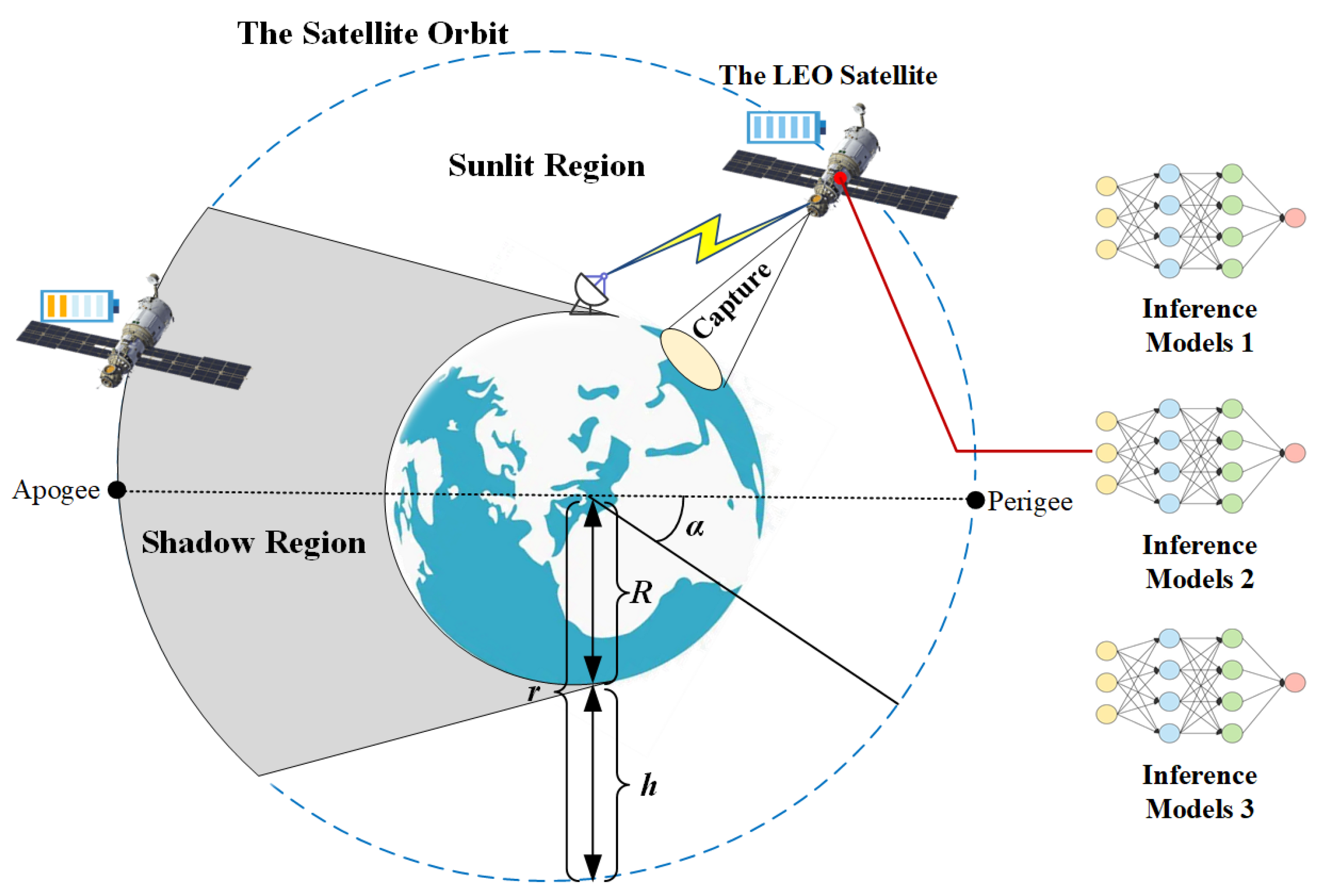
2.1. LEO-IISat Orbital Model

In Figure 1, the operational orbit of the LEO-IISat and its support for EO applications are depicted. The LEO-IISat alternately passing through sunlit and shadow regions along its orbit [19]. In both of these regions, the LEO-IISat is capable of capturing EO images and utilizing multiple inference models for data processing and inference tasks, supporting various EO applications [20].

The orbital equation of the LEO-IISat is represented as [21]:

$$r\left(t\right)=(R+h)[1-e·cos(\alpha \left(t\right)\left)\right]$$

(1)

where $r\left(t\right)$ represents the orbital radius of the LEO-IISat at a given time t, which is the distance of the satellite from the Earth’s center. R is the Earth’s radius, h is the orbital altitude, e is the orbital eccentricity, and $\alpha \left(t\right)$ is the true anomaly, which is the angle between the LEO-IISat’s current position and the perigee.

The orbital period of the LEO-IISat is given by [22]:

$$T_s=2\pi \sqrt{{\displaystyle \frac{{(R+h)}^3}{G{M}_e}}}$$

(2)

where G is the gravitational constant and $M_e$ is the Earth’s mass.

2.2. LEO-IISat Energy Model

Figure 2 illustrates the energy distribution of the LEO-IISat in both sunlit and shadow regions. In the sunlit region, the solar panels generate electricity by absorbing sunlight, and the Electrical Power System (EPS) distributes this energy to the images capture, image inference, and communication modules, enabling LEO-IISat to efficiently execute image inference tasks [23]. At the same time, the EPS stores any surplus energy in the onboard batteries. In the shadow region, where sunlight is unavailable, the power system relies on the energy stored in the onboard batteries to provide energy to all modules [24].

Let the initial battery energy of the LEO-IISat upon entering the sunlit region be $E_B^o$, the maximum battery capacity be $E_B^{\max }$, and the minimum battery energy required for LEO-IISat operation be $E_B^{\min }$. Prior to entering the shadow region, the LEO-IISat must charge its battery to $E_B^{\max }$ to ensure sufficient energy availability.

The orbital period $T_s$ is divided into N equal time slots, with $\Delta t$ representing the duration of each time interval. The sequence of time slots is denoted as $\mathcal{T}=\{t_1,\cdots ,t_i,\cdots ,t_N\}$, where $t_i$ represents any time slot.

Let $P_r\left(t\right)$ be the solar radiation received per square meter of the solar panel, given by:

$$P_r\left(t\right)=\left\{\begin{array}{cc}{P}_{max}exp\left[-{\displaystyle \frac{{(2t-\mu )}^2}{8{\sigma }^2}}\right],\hfill & 0\le t\le \mu T_s\hfill \\ 0,\hfill & \mu T_s<t\le T_s\hfill \end{array}\right.$$

(3)

where $P_{\max }$ is the peak power received per square meter, $\mu$ is the fraction of time in the sunlit region during the orbital period, and $\sigma$ is the parameter controlling radiation intensity distribution.

If $t_i$ is within the sunlit region, $1\le i\le \mu N$, the energy captured in $t_i$ is:

$$E_i^c=\eta D{\int }_{(i-1)·\Delta t}^{i·\Delta t}{P}_r\left(t\right)dt$$

(4)

where $\eta$ is the efficiency of solar energy conversion, and D is the solar panel area.

A fixed battery charging mechanism is used, where each time slot adds the same average energy to the battery. The charging energy during $t_i$ is:

$$\begin{array}{c}\hfill E_i^r={\displaystyle \frac{(E_B^{max}-E_B^o)}{\mu N}}\end{array}$$

(5)

The available energy for image inference during $t_i$ is:

$$E_i^u=E_i^c-{E_i}^r$$

(6)

If $t_i$ is within the shadow region, $\mu N<i\le N$, a cyclic averaging mechanism is used. Initially, the energy per time slot is averaged to determine the available energy for inference. After deducting the inference energy, the average is recalculated for the next slot. This process continues iteratively until the final time slot in the shadow region.

The available energy for image inference during $t_i$ is:

$$E_i^u={\displaystyle \frac{E_B^{max}-E_B^{min}-\sum _{v=\mu N}^{i-1}{E}_v}{N-i+1}}$$

(7)

where $E_v$ represents the energy consumption for any time slot from $\mu N$ to $i-1$.

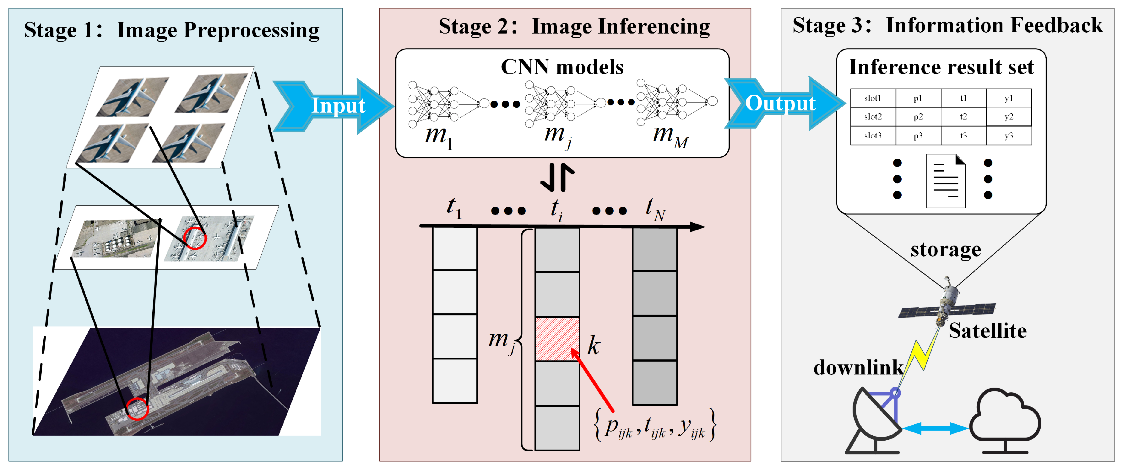
2.3. LEO-IISat Inference Model

LEO-IISat conducts EO missions based on its orbital operations, enabling real-time collection of high-resolution imagery data for aerial, maritime, and terrestrial infrastructure. This provides crucial support for achieving integrated air-sea-land traffic management [25]. To accomplish the image classification task—that is, the automatic recognition and classification of various objects in the collected images, LEO-IISat deploys M lightweight candidate CNN models, denoted as $\mathcal{M}=\{m_1,\cdots ,m_j,\cdots ,m_M\}$, where $m_j$ represents any candidate CNN model [26].

Figure 3 illustrates image inference workflow on LEO-IISat.

Stage 1: Image Preprocessing. In this stage, the LEO-IISat captures raw remote sensing images, which are subsequently segmented into smaller sub-images [27].

Stage 2: Image Inferencing. In this stage, the preprocessed sub-images are fed into the onboard candidate CNN models for analysis. These models extract images features and identify the target object categories within the images [28].

Stage 3: Information Feedback. In this stage, once the image inference process is completed, the results, which include the identified target object categories, are transmitted to the ground station for further analysis, while irrelevant information is discarded [29].

The xView dataset, a widely recognized benchmark in remote sensing images analysis, is used in this paper as the source of raw remote sensing images during the images preprocessing stage [30].

The segmentation process of the raw remote sensing images is as follows: First, a sliding window cropping technique was used to segment the raw high-resolution images (3000 × 3000 pixels) into smaller sub-images (224 × 224 pixels) [31]. Then, min-max normalization was applied to scale the pixel values of the segmented sub-images from the range [0, 255] to [0, 1], ensuring a consistent input scale across all images. To enhance the diversity of the dataset and improve the robustness of the model, random flipping and random rotation were performed during preprocessing, simulating potential images transformations encountered in real-world applications. Finally, the images were standardized using mean and standard deviation, ensuring that the pixel values for each channel follow a consistent distribution [32].

Figure 4 displays four representative target object categories from the xView dataset, covering critical categories in aerial, maritime, and terrestrial transportation [33]. The identification of fixed-wing aircraft (a) helps track air traffic and assist in aviation safety management. The recognition of ferries (b) aids in monitoring maritime traffic, optimizing ferry routes, and ensuring safe operations in port areas. For buildings (c) and storage tanks (d), LEO-IISat can identify and assess the condition of urban infrastructure and industrial sites [34].

Let the number of images to be processed at $t_i$ follow a Poisson distribution, as given by:

$$\begin{array}{c}\hfill Q(P_i=n_i)={\displaystyle \frac{e^{-{\lambda }_i}{{\lambda }_i}^{n_i}}{n_i!}}\end{array}$$

(8)

where $n_i$ represents the number of images in $t_i$, and ${\lambda }_i$ is the average number of images in $t_i$.

The sequence of images in any time slot to be processed is denoted as $\mathcal{I}=\{I_1,\cdots ,I_k,\cdots \}$, where $I_k$ represents any image.

The performance set for inferring the k-th image with model $m_j$ during $t_i$ is:

$$\begin{array}{c}\hfill {\mathcal{P}}_{\mathcal{S}}=\left\{p_{ijk},t_{ijk},y_{ijk}\right\},1\le i\le N,1\le j\le M\end{array}$$

(9)

where $p_{ijk}$ is the inference power for the k-th image during $t_i$ using $m_j$, $t_{ijk}$ is the inference time for the k-th image during $t_i$ using $m_j$, and $y_{ijk}$ is the inference result label for the k-th image during $t_i$ using $m_j$.

Figure 5 demonstrates the aforementioned performance data set ($P_{ijk}$, $t_{ijk}$, $y_{ijk}$) in a 3D coordinate system, along with its relationships to the time slots ($\mathcal{T}$), models ($\mathcal{M}$), and image sequences ($\mathcal{I}$). Here, the axes i, j, and k correspond to the time slots ($\mathcal{T}$), models ($\mathcal{M}$), and image sequences ($\mathcal{I}$), respectively.

The average image inference energy consumption using $m_j$ during $t_i$ is:

$$\begin{array}{c}\hfill \overline{E_{ij}}={\displaystyle \frac{{\displaystyle \sum _{k=1}^{n_i}}{p}_{ijk}·t_{ijk}}{n_i}},1\le i\le N,1\le j\le M\end{array}$$

(10)

The image inference accuracy using model $m_j$ during $t_i$ is:

$$\begin{array}{c}\hfill A_{ij}={\displaystyle \frac{{\displaystyle \sum _{k=1}^{n_i}}1(y_{ijk}=x_{ijk})}{n_i}}\end{array}$$

(11)

where $x_{ijk}$ is the ground truth label, $1(y_{ijk}=x_{ijk})$ is an indicator function that equals 1 if $y_{ijk}=x_{ijk}$ is satisfied, and 0 otherwise.

2.4. Problem Formulation

To quantify both accuracy and energy consumption, the $AEE$ index is defined as follows:

$$\begin{array}{c}\hfill \mathit{AEE}={\displaystyle \frac{\mathit{Accuracy}}{\mathit{Energy}}}\end{array}$$

(12)

where $Accuracy$ denote the inference accuracy (expressed as %), defined as the ratio of correctly classified images to the total number of tested images. $Energy$ represent the energy consumed during inference (measured in Joules). The $AEE$ represents the inference accuracy per unit of energy consumed, expressed in terms of Accuracy per Joule (Accuracy/Joule)

In this paper, the $AE{E}_{ij}$ is derived from the basic formula of $AEE$, representing the $AEE$ value of selecting model $m_j$ in time slot $t_i$. The formula is given by:

$$\begin{array}{c}\hfill AE{E}_{ij}={\displaystyle \frac{A_{ij}}{\overline{E_{ij}}}}={\displaystyle \frac{{\displaystyle \sum _{k=1}^{n_i}}1(y_{ijk}=x_{ijk})}{\sum _{k=1}^{n_i}(P_{ijk}·t_{ijk})}}\end{array}$$

(13)

Since our study aims for general applicability and is not focused on a specific category or domain, and the experiments are conducted on a dataset with a relatively balanced class distribution, the accuracy $A_{ij}$ represents the unweighted average across different image categories.

Assume there are two models, $m_1$ and $m_2$, which are selected in time slot $t_1$. $m_1$ has an accuracy of 92% while consuming 0.8 J of energy; $m_2$ has an accuracy of 88% while consuming 0.5 J of energy. The AEE values of $m_1$ and $m_2$ in time slot $t_1$ are represented as:

$$\begin{array}{c}\hfill AE{E}_{11}={\displaystyle \frac{0.92}{0.8}}=1.15,AE{E}_{12}={\displaystyle \frac{0.88}{0.5}}=1.76\end{array}$$

(14)

Although in time slot $t_1$, $m_1$ has a higher accuracy, its higher energy consumption results in a lower $AEE$ value compared to $m_2$, thereby highlighting the advantage of $m_2$ in time slot $t_1$.

The objective function and constraints are as follows:

$$\begin{array}{cc}\hfill & max\sum _{i=1}^N\sum _{j=1}^{M}1(m_j=m_j^{\mathrm{opt}}|t_i)·AE{E}_{ij}\hfill \end{array}$$

(15)

$$\begin{array}{cc}\hfill \mathrm{s}.\mathrm{t}.& A_{ij}\ge A_i^{min}\hfill \end{array}$$

(16)

$$\begin{array}{cc}\hfill & n_i·\overline{E_{ij}}\le E_i^u\hfill \end{array}$$

(17)

$$\begin{array}{cc}\hfill & \forall t_i,\exists !m_j\hfill \end{array}$$

(18)

where $1(m_j=m_j^{\mathrm{opt}}\mid t_i)$ is a conditional indicator function. It equals 1 if $m_j$ is optimal during $t_i$; otherwise, it is 0.

Function (16) represents the inference accuracy constraint, where $A_i^{min}$ is the minimum required inference accuracy during $t_i$. Function (17) refers to the inference energy consumption constraint. Function (18) ensures that for each $t_i$, only one model $m_j$ is selected.

2.5. Problem Solving

The overall process of our adaptive model selection strategy for satellite inference is as follows: First, we select a set of initial candidate models. Subsequently, these candidate models are trained on a unified remote sensing dataset (the xView dataset). After training, each model is evaluated on a fixed test subset of the xView dataset using key performance metrics. We formalize the model selection problem as a Markov Decision Process (MDP), treating each discrete time slot within the satellite’s orbital period as a decision point. In each time slot, a Deep Q-Network (DQN) dynamically selects the optimal model from the pre-trained candidate pool to adapt to the satellite’s current energy level, inference task requirements, and expected inference accuracy.

The above problem is modeled as a Markov Decision Process [35].

The MDP consists of the tuple $(S,A,T,r,\gamma )$:

• $S=\{E_i^u,I_i\}$ is the state space, where the state element $E_i^u$ represents the available energy for inference in $t_i$, and the state element $I_i$ represents the task distribution in $t_i$.
• $A=\mathcal{M}=\left\{m_1,···,m_j,···,m_M\right\}$ is the action space, representing the choices for the adaptive strategy, which are the different CNN models.
• $T=\{T_i^E,T_i^I\}$ is the state transition function, where $T_i^E$ represents the energy state transition function, and $T_i^I$ represents the task state transition function.
• $r(i,j)$ is the reward function, representing the reward obtained by selecting CNN model $m_j$ in $t_i$, as follows:

  $$\begin{array}{c}\hfill r(i,j)={\delta }_{1}AE{E}_{ij}+{\delta }_2(A_{ij}-A_i^{min})\end{array}$$

  (19)

  where ${\delta }_1$ is the weight coefficient for accuracy-energy efficiency, and ${\delta }_2$ is the coefficient for the deviation from the minimum accuracy.
• $\gamma$ is the discount factor, determining long-term rewards.

The MDP problem is solved using the DQN, in which the optimal strategy is learned and the optimal CNN model is selected for each time slot.

Figure 6 illustrates workflow of the MDP-DQN strategy, with the specific steps described as follows:

Step 1: Initialization. The MDP framework is initialized, including the state space ($S=\{E_i^u,I_i\}$), which represents environment states ($E_i^u$) and internal states ($I_i$); the action space ($A=\mathcal{M}$), representing all possible actions; the reward function ($r(i,j)$), which measures the feedback of actions; and the state transition function ($T=\{T_i^E,T_i^I\}$), which defines how states change based on actions.

Step 2: Input Current State into DQN. The current state $S=\{E_i^u,I_i\}$ is fed into the Deep Q-Network (DQN), representing the state of the MDP environment at time t.

Step 3: Action Selection. Based on the current state S, the DQN selects an optimal action $a\in A$ using the $ϵ$-greedy strategy to maximize the expected cumulative reward. Subsequently, the selected action a is executed, and the feedback reward $r(i,j)$ is received. The system state is then updated to $S_{t+1}$ according to the state transition function $T=\{T_i^E,T_i^I\}$.

Step 4: Execute Action and Receive Feedback. Based on the reward $r(i,j)$ and the Q-value $Q_{\mathrm{target}}(s^{\prime },a^{\prime })$ from the target Q-network, the target Q-value is calculated as follows:

$$\begin{array}{c}\hfill y=r+\gamma \underset{a^{\prime }}{max}{Q}_{\mathrm{target}}(s^{\prime },a^{\prime })\end{array}$$

(20)

where $Q_{\mathrm{target}}(s^{\prime },a^{\prime })$ is the Q-value computed by the target Q-network, and $\gamma$ is the discount factor.

Step 5: Store Experience. The experience tuple $(S_t,A_t,r_t,S_{t+1})$ (current state, action, reward, next state) is stored in the replay memory buffer for future training. Then, a batch of experiences is randomly sampled from the replay buffer, and the behavioral Q-network is trained by minimizing the mean squared error (MSE) through gradient descent. The loss function is optimized as follows [36]:

$$\begin{array}{c}\hfill \theta \leftarrow \theta -\beta {\nabla }_{\theta }\mathbb{E}\left[{\left(y-Q(s,a;\theta )\right)}^2\right]\end{array}$$

(21)

where $\theta$ represents the parameters of the Q-network, $\beta$ is the learning rate, ${\nabla }_{\theta }$ denotes the gradient with respect to the parameters $\theta$, $\mathbb{E}$ is expectation value, and $Q(s,a;\theta )$ is the Q-value function of the current Q-network.

Step 6: Experience Sampling and Training. Through continuous updates of the network parameters $\theta$, the DQN is progressively optimized to select the optimal model $m_j$ at each time step $t_i$, ensuring the maximization of the target Q-value.

Step 7: Task Completion Check. The system checks whether the task has been completed. If the task is completed, the results are output, and the process terminates. Otherwise, the state is updated, and the process returns to Step 2, continuing the loop until the task is completed.

3. Results

3.1. Simulation Parameters

Table 1. LEO-IISat parameters.

Parameter	Value	Parameter	Value
h	$500\mathrm{km}$	$\eta$	25%
$T_s$	$5670\mathrm{s}$	$P_{max}$	$1.36\mathrm{kW}$
N	30	$E_B^{max}$	$10\mathrm{kWh}$
$\mu$	$70\%$	$E_B^{min}$	$2\mathrm{kWh}$
D	$100{\mathrm{m}}^2$

presents the simulation parameters for the LEO-IISat used in Earth observation missions, with an orbital altitude h of 500 km. The orbital period $T_s$ is 5670 s, divided into 30 time slots [37]. During one orbital period, approximately 70% of the time is spent in the sunlit region. The LEO-IISat is equipped with 100 ${\mathrm{m}}^2$ solar panels, with an energy conversion efficiency of 25% [38]. The solar panels are capable of generating a peak power of $1.36\mathrm{kW}$ [39]. the maximum battery capacity $E_B^{\max }$ is $10\mathrm{kWh}$, while the minimum battery energy required for LEO-IISat operation $E_B^{\min }$ is $2\mathrm{kWh}$.

Table 2. Image inference environment parameters.

Parameter Name	Parameter Value
Candidate CNN models	MobileNet_v3; MobileNet_v2; ResNet18
Onboard computing device	NVIDIA Jetson AGX Orin
Raw image dataset	xView Dataset
Number of images processed per $t_i$	$5\times {10}^4$∼$5\times {10}^5$

summarizes the image inference environment parameters used in the LEO-IISat mission. The LEO-IISat incorporates three candidate CNN models: MobileNet_v3, MobileNet_v2, and ResNet18, selected for their low computational complexity, which makes them well-suited for resource-constrained LEO-IISat environments [40]. The onboard computing device is the NVIDIA Jetson AGX Orin. The raw images from the xView dataset are segmented into multiple sub-images in the preprocessing phase, providing input data for the simulation experiments [41]. The LEO-IISat processes between $5\times {10}^4$∼$5\times {10}^5$ images per time slot, simulating the task distribution on LEO-IISat, with the exact number depending on the complexity of the tasks and operational requirements [42].

Table 3. Comparison of Accuracy, Energy, Delay, and EDP/A of candidate CNN models.

CNN Models	Accuracy (%)	Energy (J)	Delay (ms)	EDP/A (J · ms/%)
MobileNet_v3	$85.7$∼$92.4$	$0.87$∼$1.04$	$3.5$∼$4.5$	$3.30$∼$5.46$
MobileNet_v2	$75.3$∼$91.7$	$0.79$∼$0.9$	4∼5	$3.45$∼$5.98$
ResNet18	$72.2$∼$89.5$	$0.69$∼$1.0$	6∼8	$4.63$∼$11.08$

compares the performance of candidate CNN models used in the LEO-IISat, focusing on accuracy, energy consumption, and delay, and these data serve as experimental parameters for the subsequent adaptive selection strategy in this study [43]. These performance metrics are obtained through actual measurements. The ranges for accuracy, energy consumption, and delay were obtained by testing 1000 segmented images 100 times. The ranges shown for accuracy, energy consumption, and delay represent the minimum and maximum values observed across these tests. Energy consumption is measured per image, and delay does not include any additional overhead (such as model loading time, data transmission time, etc.); it represents the pure inference delay. MobileNet_v3 offers the best accuracy with a delay ranging from 3.5 to 4.5 ms, making it ideal for tasks that require high precision and real-time performance; however, its higher energy consumption may limit its use in power-constrained LEO-IISat EO missions. In comparison, MobileNet_v2 strikes a better balance between accuracy and energy efficiency with a delay of 4 to 5 ms, making it a good choice for EO missions where some loss in accuracy is acceptable. Finally, while ResNet18 has the lowest accuracy, it is the most energy-efficient, with a delay ranging from 6 to 8 ms, making it suitable for energy-constrained EO missions where delay is not as critical.

To further evaluate these models, we introduce the Energy-Delay-Product per Accuracy (EDP/A) metric, defined as:

$$\mathit{EDP}/\mathit{A}={\displaystyle \frac{\mathit{Energy}\times \mathit{Delay}}{\mathit{Accuracy}}}$$

This metric provides a comprehensive assessment by considering the trade-off between energy consumption, processing delay, and accuracy. Lower EDP/A values indicate better overall efficiency. The EDP/A values for the three models were calculated based on the experimental data presented in Table 3.

According to the data in Table 3, we have plotted a boxplot to visually compare the performance of different CNN models across multiple metrics, including Accuracy, Energy, Delay, and EDP/A, as shown in Figure 7.

Table 4. MDP-DQN strategy parameters.

Parameter	Value	Parameter	Value	Parameter	Value
${\delta }_1$	1.5	$\kappa$	2000	$\gamma$	0.99
${\delta }_2$	10	$\beta$	0.001	$ϵ$	0.9

presents the parameters for the MDP-DQN strategy applied to LEO-IISat. Here, the weight coefficient for accuracy-energy efficiency ${\delta }_1$ is set to 1.5; the coefficient for the deviation from the minimum accuracy ${\delta }_2$ is set to 10; the number of training episodes $\kappa$ is set to 2000; the learning rate $\beta$ is set to 0.001, which helps stabilize the training process; the discount factor for future rewards $\gamma$ is set to 0.99, placing greater emphasis on future rewards; and the initial exploration rate $ϵ$ is set to 0.9, which encourages more exploration in the early stages of training [44].

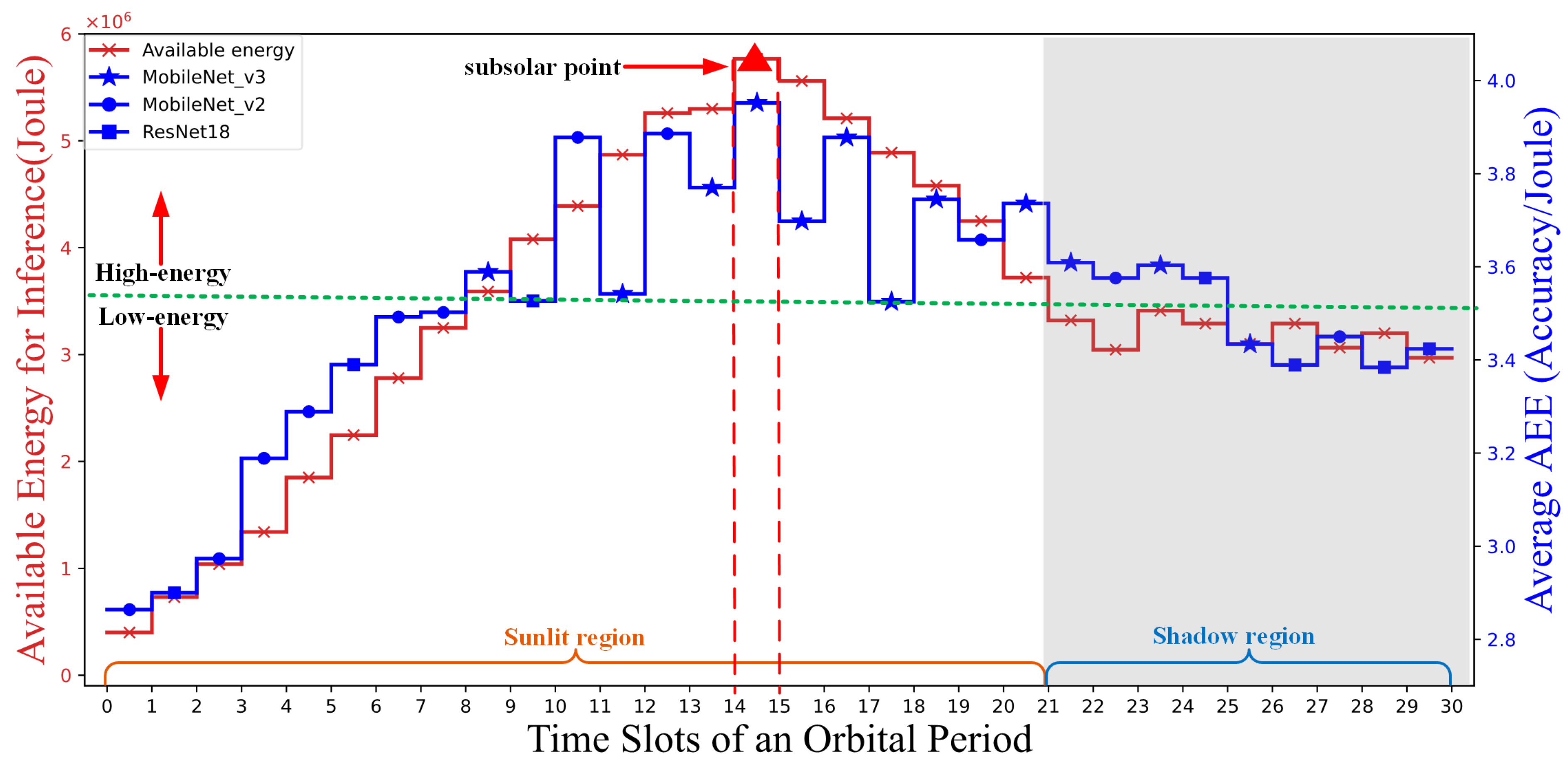
3.2. MDP-DQN Strategy Results

Figure 8 presents the curves of available energy for inference, the adaptive model selection, and the AEE index performance curves for different time slots during an orbital period. The available energy for inference first increases in the sunlight region, reaching a maximum of approximately $5.8\times {10}^6$ joules at the subsolar point (the 15th time slot), and then begins to decrease. In the shadow region, the available energy for inference remains relatively stable at approximately $3.2\times {10}^6$ joules. Under high-energy condition (i.e., $3.7\times {10}^6$∼$6\times {10}^6$ J), MobileNet_v3 is prioritized, supplemented by MobileNet_v2, with MobileNet_v3 accounting for 70% and MobileNet_v2 for 30%. Under low-energy condition (i.e., $0.4\times {10}^6$∼$3.7\times {10}^6$ J), MobileNet_v2 and ResNet18 exhibit competitiveness.

Moreover, under high-energy conditions, the transient fluctuations in model selection can be attributed to our adaptive inference strategy, which not only considers the available energy level but also accounts for variations in the number of images processed in each time slot. Changes in the number of images affect the AEE values, and since the image count in each time slot follows a Poisson distribution, occasional variations in model selection may occur even under high-energy conditions.

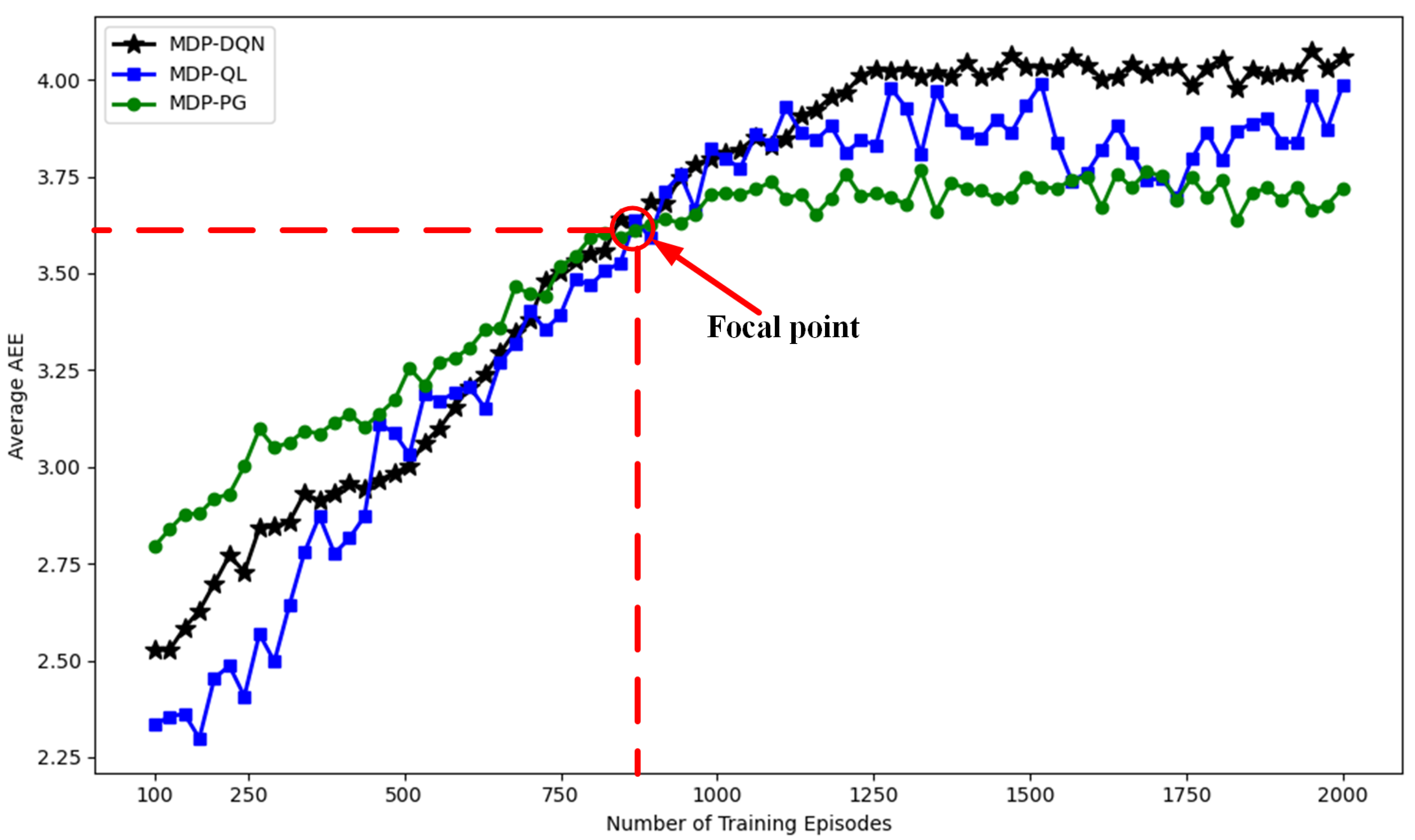
3.3. Comparison Results of Different Strategies

To validate the performance of the proposed strategy, the following baseline strategies are considered for comparison experiments, all of which are solutions based on the MDP:

• The MDP-Q Learning strategy (MDP-QL): The Q-learning updates the Q-values of state-action pairs to learn the optimal strategy [45].
• The MDP-Policy gradient strategy (MDP-PG): The policy gradient strategy directly optimizes the policy parameters to maximize cumulative rewards [46].

Both of these strategies are classical reinforcement learning algorithms widely used to solve the MDP problem [47]. They enable a comprehensive evaluation of the MDP-DQN strategy in terms of accuracy, convergence speed, and stability [48].

Figure 9 presents the relationship between the average number of images per time slot and the AEE index for different strategies. As the average number of images per time slot increases, the AEE index values of all strategies gradually decrease. This is because processing more images with the same energy supply reduces accuracy, thereby lowering the AEE index values. This indicates that in energy-limited situations, a balance between task load and model complexity is necessary. Under low-load conditions (i.e., $0.5\times {10}^5$∼$1.5\times {10}^5$), the performance gap between MDP-DQN and MDP-QL is small; however, under high-load conditions (i.e., $1.5\times {10}^5$∼$5\times {10}^5$), the MDP-DQN strategy estimates Q-values more accurately and performs better.

To quantify measurement uncertainty, we conducted 30 independent experiments under all load conditions and computed the 95% confidence intervals (CIs) using the standard error of the mean. Across all load conditions ($0.5\times {10}^5$∼$1.5\times {10}^5$), the average AEE index values are 3.31 (95% CI: 3.26–3.36) for MDP-DQN, 3.12 (95% CI: 3.07–3.17) for MDP-QL, and 2.95 (95% CI: 2.92–2.98) for MDP-PG. Consequently, MDP-DQN improves the AEE index by approximately 6.1% and 12.2% relative to MDP-QL and MDP-PG.

Figure 10 illustrates the comparison of cumulative AEE scores between the MDP-DQN adaptive strategy and the fixed model over 30 time slots within an orbital period. The MDP-DQN strategy adaptively selects among three candidate models (MobileNet_v3, MobileNet_v2, and ResNet18), while the fixed model consistently employs MobileNet_v2. The final cumulative score for the MDP-DQN adaptive strategy is 142.34, while that for the fixed model is 108.41. Therefore, compared to the fixed model, the AEE index of MDP-DQN is improved by approximately 31.3%.

Finally, we repeated the experiments of the adaptive selection strategy over 30 complete orbital cycles, and the results showed that the strategy achieved a maximum inference accuracy of 91.8% and an average inference accuracy of 89.1%.

Figure 11 illustrates the performance trends of three different algorithms (MDP-DQN, MDP-QL, and MDP-PG) as the average AEE index evolves with the increase in training episodes. The x-axis represents the number of training episodes, while the y-axis measures the algorithm’s performance metric—average AEE index. Overall, as the number of training episodes increases, the performance of all algorithms improves, but their improvement rates, final performance, and stability exhibit noticeable differences. A critical focal point is observed at approximately (860, 3.62), where the performance of all three algorithms converges. At this stage, the average AEE index values of MDP-DQN, MDP-QL, and MDP-PG are similar, indicating a transitional phase in their performance trends. Beyond this focal point, the trajectories of the algorithms diverge significantly. From the analysis, MDP-PG performs best in the early training phase (0–500 episodes), with rapid and stable increases in average AEE index. However, after the focal point, its performance plateaus, with no significant improvement. In contrast, MDP-DQN demonstrates superior performance in the middle and late stages of training, eventually stabilizing at the highest average AEE index value, making it the most effective algorithm among the three. Additionally, while MDP-QL shows rapid improvement, it suffers from high volatility throughout the training process, particularly beyond the focal point, indicating a lack of stability.

Table 5. Comparison of the average variance values of three strategies during training.

Strategies	MDP-DQN	MDP-QL	MDP-PG
Variance	0.023	0.061	0.032

compares the variance of the AEE index across the three strategies (MDP-DQN, MDP-QL, and MDP-PG) during training, with the variance calculated based on the average of the previous and next sampling points (as shown in Figure 11). As shown in Table 5, MDP-DQN exhibits the lowest variance and higher stability. The fluctuations in the training process are mainly due to two factors: first, the transitional regions between sunlit and shadow lead to abnormal energy fluctuations; second, the number of images processed in each time slot varies irregularly.

Figure 12 shows the Average AEE index of MDP-DQN, MDP-QL, and MDP-PG under different learning rates and discount factors. The left panel (a) illustrates the Average AEE index of the algorithms under varying learning rates (${10}^{-4}$ to ${10}^{-2}$). MDP-DQN achieves its highest AEE index at a learning rate of ${10}^{-3}$, marked as the Optimal Point. MDP-QL and MDP-PG remain relatively stable and exhibit lower AEE index values compared to MDP-DQN.The right panel (b) presents the Average AEE index under different discount factors (0.90 to 1.00). MDP-DQN achieves its optimal value near a discount factor of 1.0, marked again as the Optimal Point. MDP-QL shows a consistent trend across all discount factors, while MDP-PG demonstrates a slight upward trend as the discount factor increases.

Figure 13 illustrates the normalized performance comparison of MDP-DQN, MDP-QL, and MDP-PG across four key metrics: AEE index, stability, memory usage, and training time. MDP-DQN excels in AEE index and stability, indicating high accuracy and robustness, but incurs higher memory usage and training time. MDP-QL shows balanced performance across all metrics, while MDP-PG performs efficiently in memory usage and training time, but lags behind in AEE index and stability. This visualization highlights the trade-offs among the algorithms for different application priorities.

Table 6. Time complexity analysis of algorithms.

Algorithms	DQN	QL	PG
Time complexity	$O(L\times N_e^2)$	$O\left(\right|S|\times |A\left|\right)$	$O(L\times N_e^2)$

presents the time complexity of the three algorithms, where L is the number of network layers, $N_e$ is the number of neurons per layer, $\left|S\right|$ is the size of the state space, and $\left|A\right|$ is the size of the action space. Both the MDP-DQN and the MDP-PG use deep neural networks, resulting in a similar time complexity of $O(L\times {N_e}^2)$ [49]. As the complexity of the network structures increases, so does the time complexity. In contrast, the MDP-QL has a time complexity of $O\left(\right|S|\times |A\left|\right)$, directly related to the size of the state and action spaces [50]. This algorithm performs well when the state and action spaces are small, but the computing load increases as these spaces expand.

4. Discussion

From an overall perspective, the AEE index value shows a positive correlation with the available energy for inference. But under high energy condition, the AEE index performance of the models fluctuates significantly, reaching a maximum of approximately 3.94 and a minimum of 3.42. This is due to variations in the number of images (as illustrated in Figure 8) and the tendency to select complex models with numerous parameters and high-dimensional features, making them more susceptible to randomness and noise.

During the Table 3 evaluation, MobileNet_v3 demonstrated excellent accuracy (85.7% to 92.4%), making it particularly suitable for complex and high-precision task scenarios, such as disaster detection or urban development monitoring. While its energy consumption (0.87 to 1.04 J/image) was slightly higher, its performance on the Jetson AGX Orin remained highly efficient, making it ideal for high-performance operational modes. In contrast, MobileNet_v2 achieved high classification accuracy (75.3% to 91.7%) with lower energy consumption (0.79 to 0.9 J/image), making it an ideal choice for resource-constrained tasks, such as micro-satellite missions or scenarios requiring continuous operation over extended periods. Meanwhile, ResNet18 exhibited balanced performance in terms of energy consumption (0.69 to 1.0 J/image) and accuracy (72.2% to 89.5%), making it suitable for large-scale, rapid screening tasks or secondary tasks requiring high real-time processing efficiency [51].

From the results presented in Table 4 and Figure 12, it is evident that the performance of the DQN algorithm is highly sensitive to key parameters, such as learning rate and discount factor. Regarding the impact of the learning rate, DQN achieves optimal energy efficiency (maximum AEE) when the learning rate is set to ${10}^{-3}$, indicating that this value strikes a balance between stable convergence and rapid updates. In contrast, higher learning rates (e.g., ${10}^{-1}$) result in a decline in performance, potentially due to unstable convergence caused by overly aggressive parameter updates. Additionally, in terms of the discount factor, DQN performs best at $\gamma =0.99$, demonstrating its ability to balance short-term and long-term rewards during the optimization process [52]. This also highlights DQN’s advantage in handling long-term temporal dependencies in complex tasks. In comparison, the performance of QL and PG shows less sensitivity to these parameters but remains significantly inferior to DQN overall. These results further underscore the superiority of deep reinforcement learning in energy efficiency optimization and decision-making accuracy, particularly in resource-constrained environments such as satellite edge computing networks [53].

From Figure 11, it is evident that MDP-DQN excels in the later stages of training, making it well-suited for tasks that require high stability and optimal final performance. This robust performance can be attributed to the incorporation of experience replay and target network mechanisms, which help smooth out fluctuations in Q-value estimates as training progresses. In contrast, MDP-PG demonstrates rapid convergence during the initial phase, rendering it more suitable for scenarios that demand quick progress. However, its performance tends to plateau in later stages, suggesting that further tuning may be necessary to maintain long-term stability. Meanwhile, MDP-QL shows rapid improvement at the outset but suffers from significant volatility throughout the training process, likely due to challenges inherent in Q-learning when operating in high-dimensional state spaces. This indicates that MDP-QL might benefit from additional modifications or adaptive parameter adjustments to achieve a stability level comparable to that of MDP-DQN.

The training process of MDP-DQN exhibits a certain degree of volatility. As shown in Figure 6, the training relies on several random factors: the intermittent energy supply of the satellite introduces randomness in state transitions, and fluctuations in the number of input data within each time slot result in inherent uncertainty in the reward feedback. However, optimizing the learning rate and discount factor can help the model better cope with these random factors in the environment. Therefore, to overcome these issues and stabilize the training process, we selected the optimal learning rate and discount factor as the experimental parameters for the adaptive selection strategy, as illustrated in Figure 12. Finally, based on the convergence trend shown in Figure 11, MDP-DQN has essentially converged after approximately 1200 training episodes, exhibiting minimal fluctuations with a variance of 0.023.

5. Conclusions

This paper introduces the AEE index to quantify inference accuracy unit of energy consumption and evaluate the inference performance of LEO-IISat. The proposed MDP-DQN strategy successfully integrates lightweight models and adaptive inference frameworks, dynamically balancing computational and energy resources to address the challenges in LEO-IISat for EO missions. The simulation results demonstrate the superiority of this strategy, achieving a 31.3% improvement in inference performance compared to a fixed model strategy at the same energy consumption, and achieves improvements over MDP-PG and MDP-QL strategies, enhancing the AEE index by 12.2% and 6.09%, respectively.

The MDP-DQN strategy has substantial applications in real-time disaster monitoring, precise climate analysis, and military reconnaissance. Future research will focus on improving CNN architectures to adapt to diverse mission scenarios, optimizing real-time images batch processing techniques, and enhancing system robustness under dynamic task conditions. These advancements will further solidify the role of LEO-IISat as a cornerstone for next-generation EO missions.

References

1. Banafaa, M.; Shayea, I.; Din, J.; Azmi, M.H.; Alashbi, A.; Daradkeh, Y.I.; Alhammadi, A. 6G Mobile Communication Technology: Requirements, Targets, Applications, Challenges, Advantages, and Opportunities. Alex. Eng. J. 2023, 64, 245–274. [Google Scholar] [CrossRef]
2. Dwivedi, Y.K.; Hughes, L.; Ismagilova, E.; Aarts, G.; Coombs, C.; Crick, T.; Duan, Y.; Dwivedi, R.; Edwards, J.; Eirug, A.; et al. Artificial Intelligence (AI): Multidisciplinary Perspectives on Emerging Challenges, Opportunities, and Agenda for Research, Practice, and Policy. Int. J. Inf. Manag. 2021, 57, 101994. [Google Scholar] [CrossRef]
3. Bedi, R. In-Orbit Artificial Intelligence and Machine Learning On-Board Processing Solutions for Space Applications: Edge-Based and Versal Space Reference Designs: First Design-In Experiences. In Proceedings of the 2023 European Data Handling & Data Processing Conference (EDHPC), Juan Les Pins, France, 2–6 October 2023; pp. 1–4. [Google Scholar] [CrossRef]
4. He, C.; Dong, Y.; Li, H.; Liew, Y. Reasoning-Based Scheduling Method for Agile Earth Observation Satellite with Multi-Subsystem Coupling. Remote Sens. 2023, 15, 1577. [Google Scholar] [CrossRef]
5. Cui, G.; Duan, P.; Xu, L.; Wang, W. Latency Optimization for Hybrid GEO–LEO Satellite-Assisted IoT Networks. IEEE Internet Things J. 2023, 10, 6286–6297. [Google Scholar] [CrossRef]
6. Zhu, X.; Jiang, C. Integrated Satellite-Terrestrial Networks toward 6G: Architectures, Applications, and Challenges. IEEE Internet Things J. 2021, 9, 437–461. [Google Scholar] [CrossRef]
7. Wang, W.; Chen, W.; Luo, Y.; Long, Y.; Lin, Z.; Zhang, L.; Lin, B.; Cai, D.; He, X. Model Compression and Efficient Inference for Large Language Models: A Survey. arXiv 2024, arXiv:2402.09748. [Google Scholar] [CrossRef]
8. Malaviya, P.; Sarvaiya, V.; Shah, A.; Thakkar, D.; Shah, M. A Comprehensive Review on Space Solar Power Satellite: An Idiosyncratic Approach. Environ. Sci. Pollut. Res. 2022, 29, 42476–42492. [Google Scholar] [CrossRef]
9. Miralles, P.; Thangavel, K.; Scannapieco, A.F.; Jagadam, N.; Baranwal, P.; Faldu, B.; Abhang, R.; Bhatia, S.; Bonnart, S.; Bhatnagar, I.; et al. A Critical Review on the State-of-the-Art and Future Prospects of Machine Learning for Earth Observation Operations. Adv. Space Res. 2023, 71, 4959–4986. [Google Scholar] [CrossRef]
10. Shang, S.; Zhang, J.; Wang, X.; Wang, X.; Li, Y.; Li, Y. Faster and Lighter Meteorological Satellite Image Classification by a Lightweight Channel-Dilation-Concatenation Net. IEEE J. Sel. Top. Appl. Earth Obs. Remote Sens. 2023, 16, 2301–2317. [Google Scholar] [CrossRef]
11. Leyva-Mayorga, I.; Martinez-Gost, M.; Moretti, M.; Pérez-Neira, A.; Vázquez, M.Á; Popovski, P.; Soret, B. Satellite Edge Computing for Real-Time and Very-High Resolution Earth Observation. IEEE Trans. Commun. 2023, 71, 6180–6194. [Google Scholar] [CrossRef]
12. Gost, M.M.; Leyva-Mayorga, I.; Pérez-Neira, A.; Vázquez, M.Á.; Soret, B.; Moretti, M. Edge Computing and Communication for Energy-Efficient Earth Surveillance with LEO Satellites. In Proceedings of the 2022 IEEE International Conference on Communications Workshops (ICC Workshops), Seoul, Republic of Korea, 16–20 May 2022; pp. 556–561. [Google Scholar] [CrossRef]
13. Khalek, N.A.; Tashman, D.H.; Hamouda, W. Advances in machine learning-driven cognitive radio for wireless networks: A survey. IEEE Commun. Surv. Tutor. 2024, 26, 1201–1237. [Google Scholar] [CrossRef]
14. Yin, L.; Cao, X. Inspired lightweight robust quantum Q-learning for smart generation control of power systems. Appl. Soft Comput. 2022, 131, 109804. [Google Scholar] [CrossRef]
15. Bhandari, J.; Russo, D. Global optimality guarantees for policy gradient methods. Oper. Res. 2024, 72, 1906–1927. [Google Scholar] [CrossRef]
16. Ali, Y.A.; Awwad, E.M.; Al-Razgan, M.; Maarouf, A. Hyperparameter search for machine learning algorithms for optimizing the computational complexity. Processes 2023, 11, 349. [Google Scholar] [CrossRef]
17. Wang, Z.; Zhao, W.; Zhai, A.; He, P.; Wang, D. DQN based single-pixel imaging. Opt. Express 2021, 29, 15463–15477. [Google Scholar] [CrossRef]
18. Luo, J.; Li, F.; Jiao, J. A dynamic multiobjective recommendation method based on soft actor-critic with discrete actions. J. King Saud Univ. Comput. Inf. Sci. 2025, 37, 1. [Google Scholar] [CrossRef]
19. Alavipanah, S.K.; Karimi Firozjaei, M.; Sedighi, A.; Fathololoumi, S.; Zare Naghadehi, S.; Saleh, S.; Naghdizadegan, M.; Gomeh, Z.; Arsanjani, J.J.; Makki, M.; et al. The Shadow Effect on Surface Biophysical Variables Derived from Remote Sensing: A Review. Land 2022, 11, 2025. [Google Scholar] [CrossRef]
20. Persello, C.; Wegner, J.D.; Hänsch, R.; Tuia, D.; Ghamisi, P.; Koeva, M.; Camps-Valls, G. Deep Learning and Earth Observation to Support the Sustainable Development Goals: Current Approaches, Open Challenges, and Future Opportunities. IEEE Geosci. Remote Sens. Mag. 2022, 10, 172–200. [Google Scholar] [CrossRef]
21. Wang, Z.; Li, Z.; Wang, L.; Wang, N.; Yang, Y.; Li, R.; Zhang, Y.; Liu, A.; Yuan, H.; Hoque, M. Comparison of the Real-Time Precise Orbit Determination for LEO between Kinematic and Reduced-Dynamic Modes. Measurement 2022, 187, 110224. [Google Scholar] [CrossRef]
22. Prol, F.S.; Ferre, R.M.; Saleem, Z.; Välisuo, P.; Pinell, C.; Lohan, E.S.; Elsanhoury, M.; Elmusrati, M.; Islam, S.; Çelikbilek, K.; et al. Position, Navigation, and Timing (PNT) through Low Earth Orbit (LEO) Satellites: A Survey on Current Status, Challenges, and Opportunities. IEEE Access 2022, 10, 83971–84002. [Google Scholar] [CrossRef]
23. Liu, W.; Lai, Z.; Wu, Q.; Li, H.; Zhang, Q.; Li, Z.; Li, Y.; Liu, J. In-Orbit Processing or Not? Sunlight-Aware Task Scheduling for Energy-Efficient Space Edge Computing Networks. In Proceedings of the IEEE INFOCOM 2024—IEEE Conference on Computer Communications, Vancouver, BC, Canada, 20–23 May 2024; pp. 881–890. [Google Scholar] [CrossRef]
24. Pathak, A.D.; Saha, S.; Bharti, V.K.; Gaikwad, M.M.; Sharma, C.S. A Review on Battery Technology for Space Application. J. Energy Storage 2023, 61, 106792. [Google Scholar] [CrossRef]
25. Hong, D.; Hu, J.; Yao, J.; Chanussot, J.; Zhu, X.X. Multimodal remote sensing benchmark datasets for land cover classification with a shared and specific feature learning model. ISPRS J. Photogramm. Remote Sens. 2021, 178, 107–122. [Google Scholar] [CrossRef] [PubMed]
26. Chen, Z.; Jiang, Y.; Zhang, X.; Zheng, R.; Qiu, R.; Sun, Y.; Zhao, C.; Shang, H. ResNet18DNN: Prediction Approach of Drug-Induced Liver Injury by Deep Neural Network with ResNet18. Brief. Bioinform. 2022, 23, bbab503. [Google Scholar] [CrossRef]
27. Kazmi Policht, N.F.; Brooks, T.N.; North, P. Characterization and Classification of Low-Resolution LEO and GEO Satellites with Electro-Optical Fiducial Markers. In Proceedings of the AIAA SCITECH 2024 Forum, Orlando, FL, USA, 8–12 January 2024; p. 2267. [Google Scholar] [CrossRef]
28. Abraham, K.; Abdelwahab, M.; Abo-Zahhad, M. Classification and Detection of Natural Disasters Using Machine Learning and Deep Learning Techniques: A Review. Earth Sci. Inform. 2024, 17, 869–891. [Google Scholar] [CrossRef]
29. Meimetis, D.; Papaioannou, S.; Katsoni, P.; Lappas, V. An Architecture for Early Wildfire Detection and Spread Estimation Using Unmanned Aerial Vehicles, Base Stations, and Space Assets. Drones Auton. Veh. 2024, 1, 10006. [Google Scholar] [CrossRef]
30. Sun, X.; Wang, P.; Yan, Z.; Xu, F.; Wang, R.; Diao, W.; Chen, J.; Li, J.; Feng, Y.; Xu, T.; et al. FAIR1M: A Benchmark Dataset for Fine-Grained Object Recognition in High-Resolution Remote Sensing Imagery. ISPRS J. Photogramm. Remote Sens. 2022, 184, 116–130. [Google Scholar] [CrossRef]
31. Turkoglu, M.O.; D’Aronco, S.; Perich, G.; Liebisch, F.; Streit, C.; Schindler, K.; Wegner, J.D. Crop Mapping from Image Time Series: Deep Learning with Multi-Scale Label Hierarchies. Remote Sens. Environ. 2021, 264, 112603. [Google Scholar] [CrossRef]
32. Yousif, M.J. Enhancing the accuracy of image classification using deep learning and preprocessing methods. Artif. Intell. Robot. Dev. J. 2023, 3, 348. [Google Scholar] [CrossRef]
33. Lam, D.; Kuzma, R.; McGee, K.; Dooley, S.; Laielli, M.; Klaric, M.; Bulatov, Y.; McCord, B. xView: Objects in Context in Overhead Imagery. arXiv 2018, arXiv:1802.07856. [Google Scholar] [CrossRef]
34. Qiao, Y.; Teng, S.; Luo, J.; Sun, P.; Li, F.; Tang, F. On-Orbit DNN Distributed Inference for Remote Sensing Images in Satellite Internet of Things. IEEE Internet Things J. 2024, 12, 5687–5703. [Google Scholar] [CrossRef]
35. He, Z.; Tran, K.P.; Thomassey, S.; Zeng, X.; Xu, J.; Yi, C. Multi-Objective Optimization of the Textile Manufacturing Process Using Deep-Q-Network Based Multi-Agent Reinforcement Learning. J. Manuf. Syst. 2022, 62, 939–949. [Google Scholar] [CrossRef]
36. Park, S.; Yoo, Y.; Pyo, C.W. Applying DQN Solutions in Fog-Based Vehicular Networks: Scheduling, Caching, and Collision Control. Veh. Commun. 2022, 33, 100397. [Google Scholar] [CrossRef]
37. Edwards, M.R.; Holloway, T.; Pierce, R.B.; Blank, L.; Broddle, M.; Choi, E.; Duncan, B.N.; Esparza, Á.; Falchetta, G.; Fritz, M.; et al. Satellite Data Applications for Sustainable Energy Transitions. Front. Sustain. 2022, 3, 910924. [Google Scholar] [CrossRef]
38. Myyas, R.E.N.; Al-Dabbasa, M.; Tostado-Véliz, M.; Jurado, F. A Novel Solar Panel Cleaning Mechanism to Improve Performance and Harvesting Rainwater. Solar Energy 2022, 237, 19–28. [Google Scholar] [CrossRef]
39. Chen, H.; Zhang, X.; Wang, L.; Xing, L.; Pedrycz, W. Resource-Constrained Self-Organized Optimization for Near-Real-Time Offloading Satellite Earth Observation Big Data. Knowl.-Based Syst. 2022, 253, 109496. [Google Scholar] [CrossRef]
40. Chen, B.; Liu, L.; Zou, Z.; Shi, Z. Target Detection in Hyperspectral Remote Sensing Image: Current Status and Challenges. Remote Sens. 2023, 15, 3223. [Google Scholar] [CrossRef]
41. Ferreira, B.; Silva, R.G.; Iten, M. Earth Observation Satellite Imagery Information-Based Decision Support Using Machine Learning. Remote Sens. 2022, 14, 3776. [Google Scholar] [CrossRef]
42. Zhou, X.; Liang, W.; Yan, K.; Li, W.; Wang, K.I.K.; Ma, J.; Jin, Q. Edge-Enabled Two-Stage Scheduling Based on Deep Reinforcement Learning for Internet of Everything. IEEE Internet Things J. 2022, 10, 3295–3304. [Google Scholar] [CrossRef]
43. Yang, Z.; Wang, T.; Lin, Y.; Chen, Y.; Zeng, H.; Pei, J.; Wang, J.; Liu, X.; Zhou, Y.; Zhang, J.; et al. A Vision Chip with Complementary Pathways for Open-World Sensing. Nature 2024, 629, 1027–1033. [Google Scholar] [CrossRef]
44. Yang, X.; Shi, Y.; Liu, W.; Ye, H.; Zhong, W.; Xiang, Z. Global Path Planning Algorithm Based on Double DQN for Multi-Tasks Amphibious Unmanned Surface Vehicle. Ocean Eng. 2022, 266, 112809. [Google Scholar] [CrossRef]
45. Tan, T.; Xie, H.; Xia, Y.; Shi, X.; Shang, M. Adaptive Moving Average Q-Learning. Knowl. Inf. Syst. 2024, 66, 7389–7417. [Google Scholar] [CrossRef]
46. Huang, C.; Wang, G.; Zhou, Z.; Zhang, R.; Lin, L. Reward-Adaptive Reinforcement Learning: Dynamic Policy Gradient Optimization for Bipedal Locomotion. IEEE Trans. Pattern Anal. Mach. Intell. 2022, 45, 7686–7695. [Google Scholar] [CrossRef]
47. Shakya, A.K.; Pillai, G.; Chakrabarty, S. Reinforcement Learning Algorithms: A Brief Survey. Expert Syst. Appl. 2023, 231, 120495. [Google Scholar] [CrossRef]
48. Li, D.; Yang, Q.; Ma, L.; Wang, Y.; Zhang, Y.; Liao, X. An Electrical Vehicle-Assisted Demand Response Management System: A Reinforcement Learning Method. Front. Energy Res. 2023, 10, 1071948. [Google Scholar] [CrossRef]
49. Vashist, A.; Shanmugham, S.V.V.; Ganguly, A.; Manoj, S. DQN Based Exit Selection in Multi-Exit Deep Neural Networks for Applications Targeting Situation Awareness. In Proceedings of the 2022 IEEE International Conference on Consumer Electronics (ICCE), Las Vegas, NV, USA, 7–9 January 2022; pp. 1–6. [Google Scholar] [CrossRef]
50. Rodrigues, F.F.C. Supergame, A System with Data Collection to Support Game Recommendation: Creating a Recommender System for Casual Games. Master’s Thesis, Universidade de Evora, Évora, Portugal, 2023. [Google Scholar]
51. Goriparthi, R.G. Deep Learning Architectures for Real-Time Image Recognition: Innovations and Applications. Rev. Intel. Artif. Med. 2024, 15, 880–907. Available online: https://redcrevistas.com/index.php/Revista/article/view/219 (accessed on 14 February 2025).
52. Zhang, Y.; Cheng, Y.; Zheng, H.; Tao, F. Long-/Short-Term Preference Based Dynamic Pricing and Manufacturing Service Collaboration Optimization. IEEE Trans. Ind. Inform. 2022, 18, 8948–8956. [Google Scholar] [CrossRef]
53. Nabi, A.; Baidya, T.; Moh, S. Comprehensive Survey on Reinforcement Learning-Based Task Offloading Techniques in Aerial Edge Computing. Internet Things 2024, 28, 101342. [Google Scholar] [CrossRef]
Figure 1. LEO-IISat operational orbit and EO application support.
Remotesensing 17 01175 g001
Figure 2. LEO-IISat energy distribution in sunlit and shadow regions.
Remotesensing 17 01175 g002
Figure 3. Image inference workflow on LEO-IISat.
Remotesensing 17 01175 g003
Figure 4. Representative target object categories from the xView dataset.
Remotesensing 17 01175 g004
Figure 5. The performance data set for inferring in a 3D coordinate system.
Remotesensing 17 01175 g005
Figure 6. MDP-DQN strategy workflow.
Remotesensing 17 01175 g006
Figure 7. Comparison of CNN model performance across multiple metrics.
Remotesensing 17 01175 g007
Figure 8. Available inference energy versus average AEE index in different time slots of an orbital period, and only one model is selected per time slot.
Remotesensing 17 01175 g008
Figure 9. Average number of images per slot versus average AEE index for different strategies.
Remotesensing 17 01175 g009
Figure 10. Comparison of cumulative AEE scores between the MDP-DQN adaptive strategy and the fixed model over orbital period time slots.
Remotesensing 17 01175 g010
Figure 11. Different training episodes versus average AEE index for different strategies.
Remotesensing 17 01175 g011
Figure 12. Average AEE index under different learning rates and discount factors for different strategies.
Remotesensing 17 01175 g012
Figure 13. Normalized performance comparison of different strategies across four key metrics.
Remotesensing 17 01175 g013