The Application of the Convective–Stratiform Classification Algorithm for Feature Detection in Polarimetric Radar Variables and QPE Retrieval During Warm-Season Convection


Abstract
1. Introduction
2. Data and Methods
2.1. Data
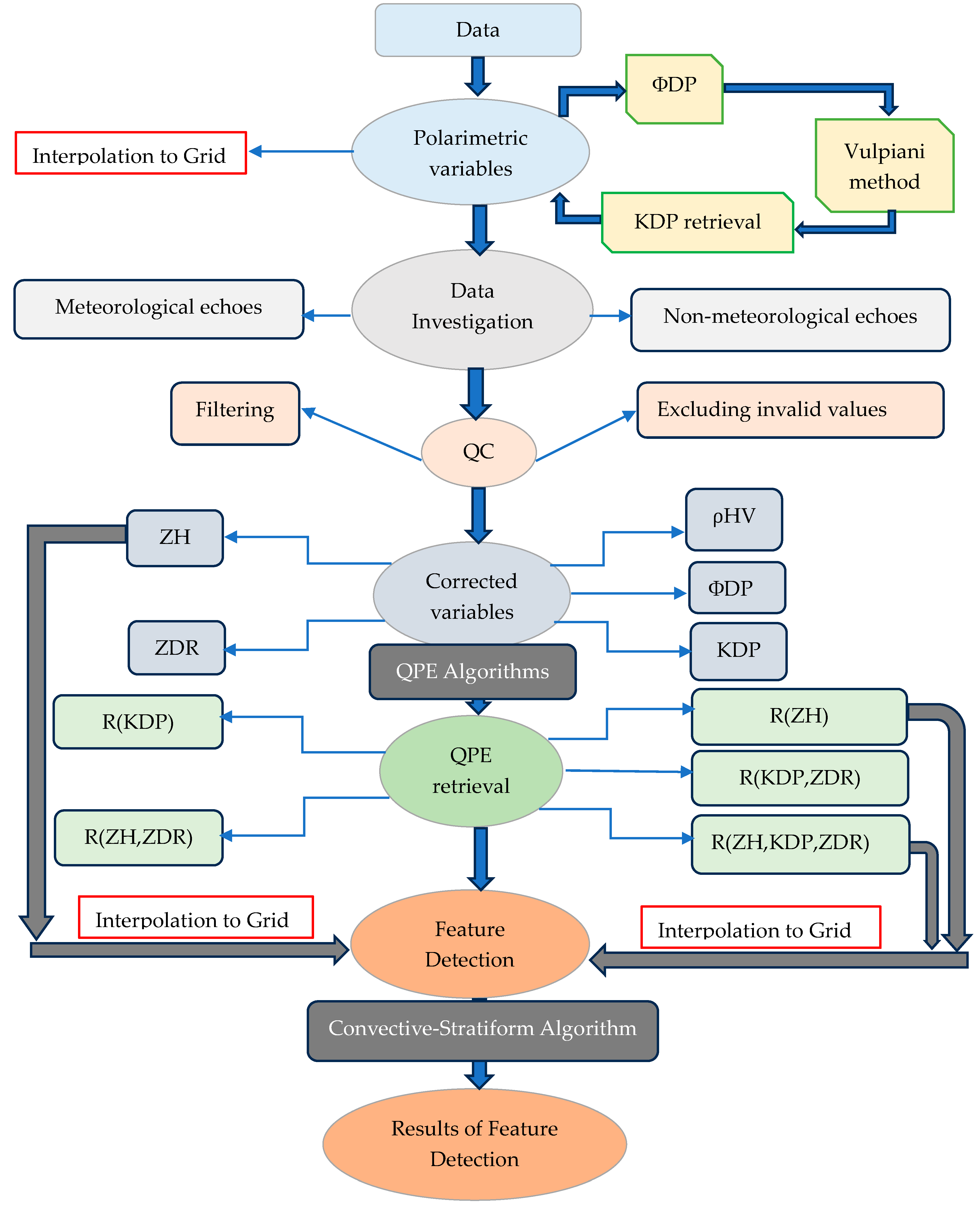
2.2. Methodology
2.2.1. Polarimetric Radar Variables Description
2.2.2. Specific Differential Phase Retrieval
2.2.3. Description of Meteorological and Non-Meteorological Echoes
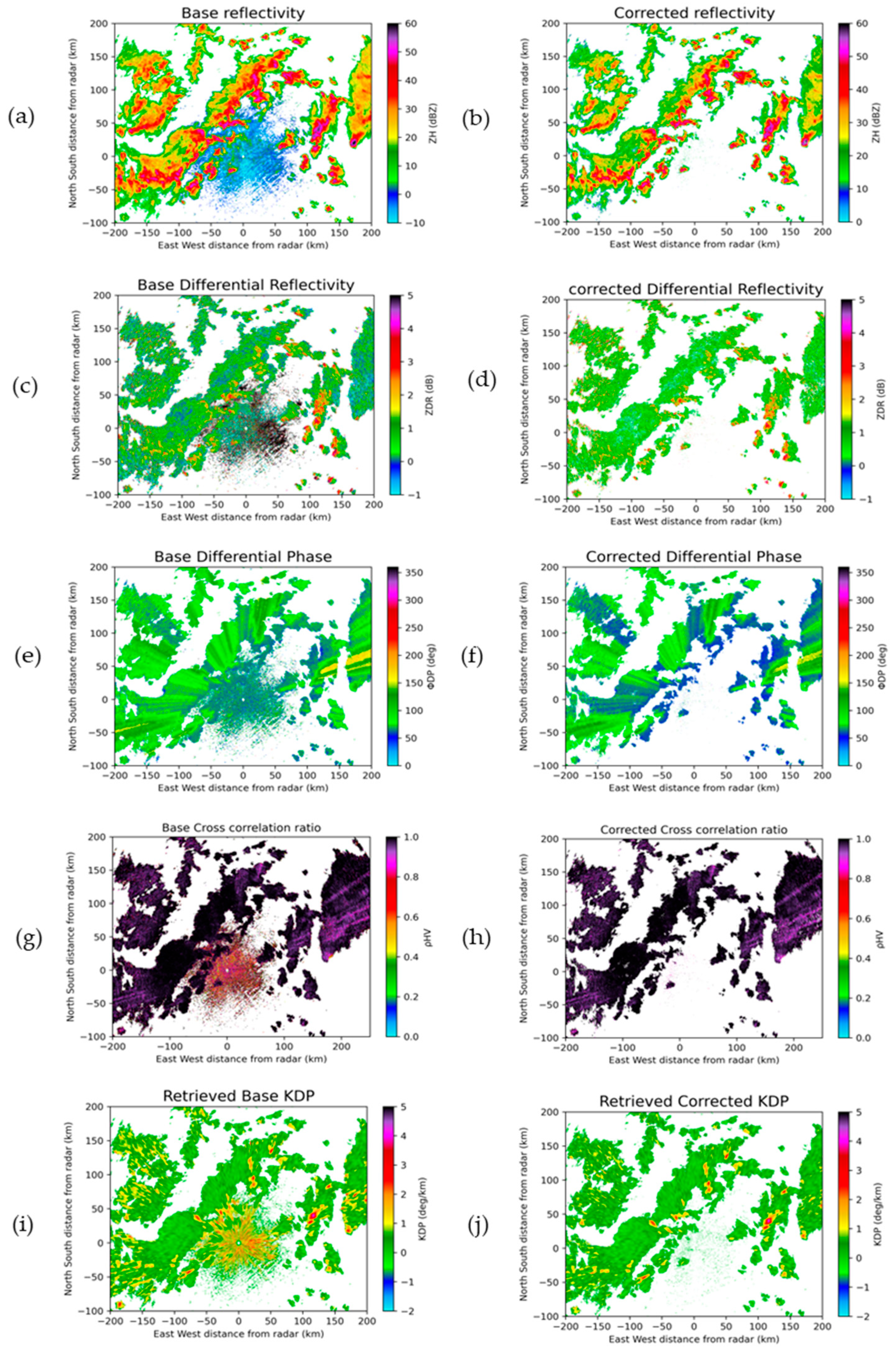
2.2.4. Quality Control of the Base Data to Filter Non-Meteorological Echoes
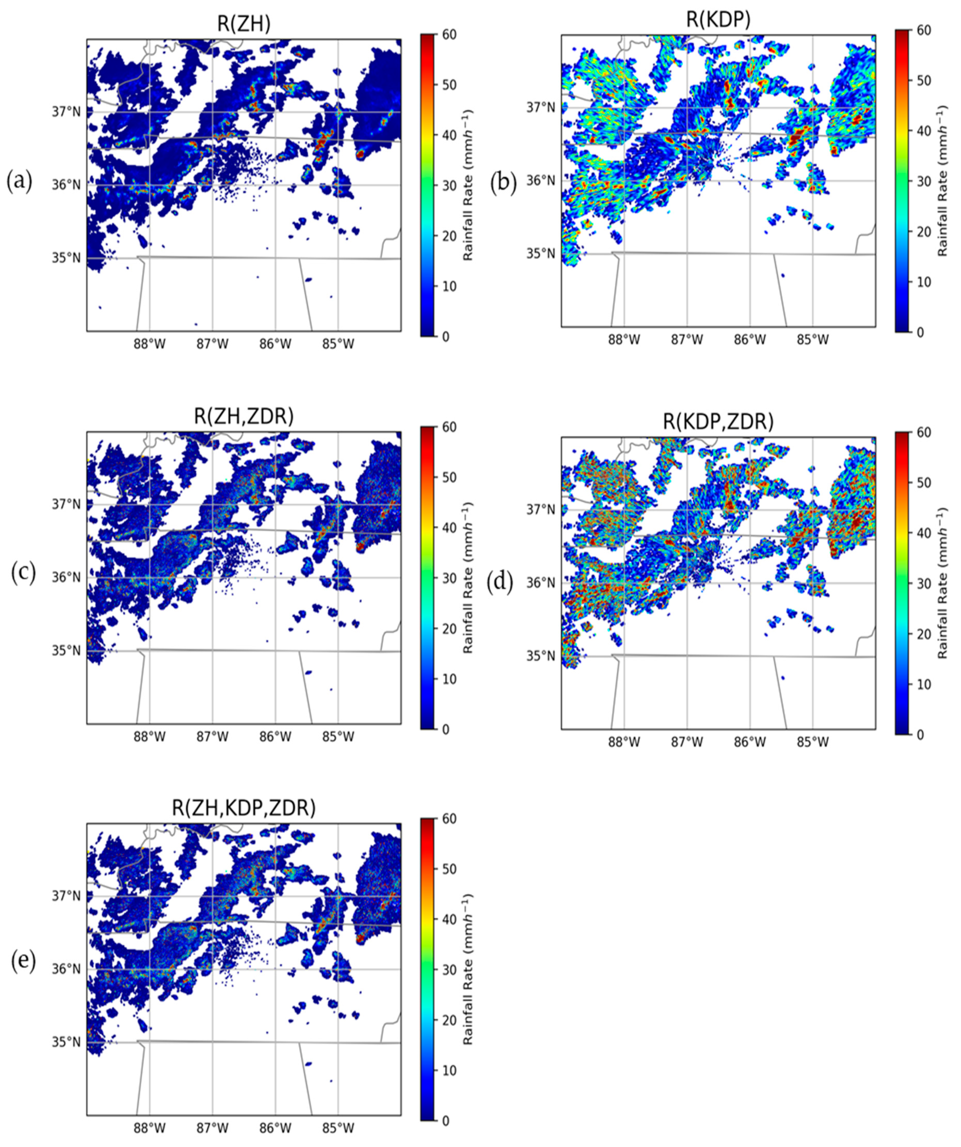
2.2.5. QPE Retrieval
2.2.6. Interpolation of Radar Data into Cartesian Grid
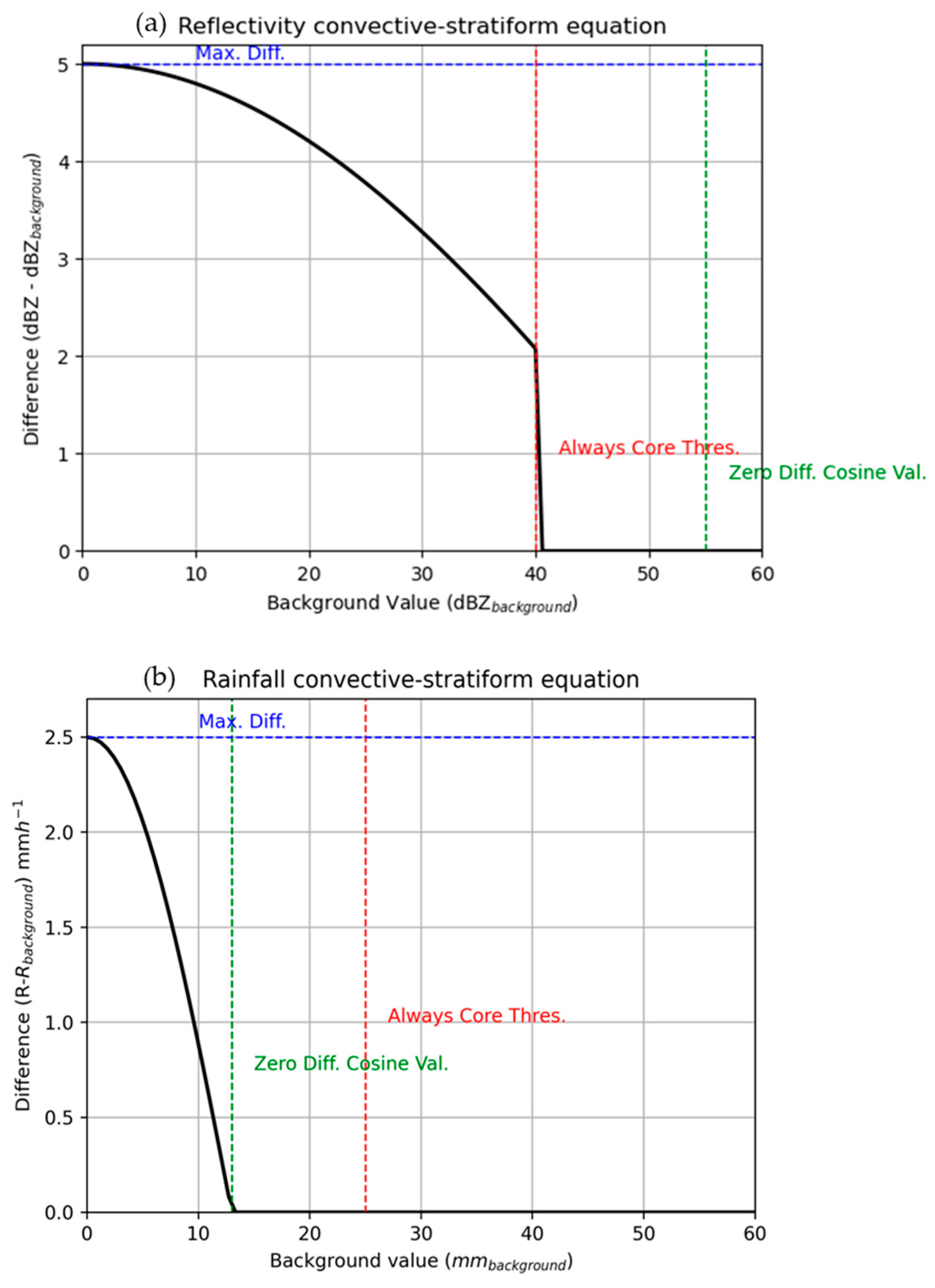
2.2.7. Feature Detection Algorithm
3. Results
3.1. Interrelationships Among the Polarimetric Variables to Discriminate Different Precipitation Types in the Radar Resolution Volume During the Event
3.2. The Role of Polarimetric Radar Variables in Distinguishing Observed Meteorological and Non-Meteorological Echoes in the Radar Resolution Volume During the Event
3.3. The Results of QPE Retrieval During the Event
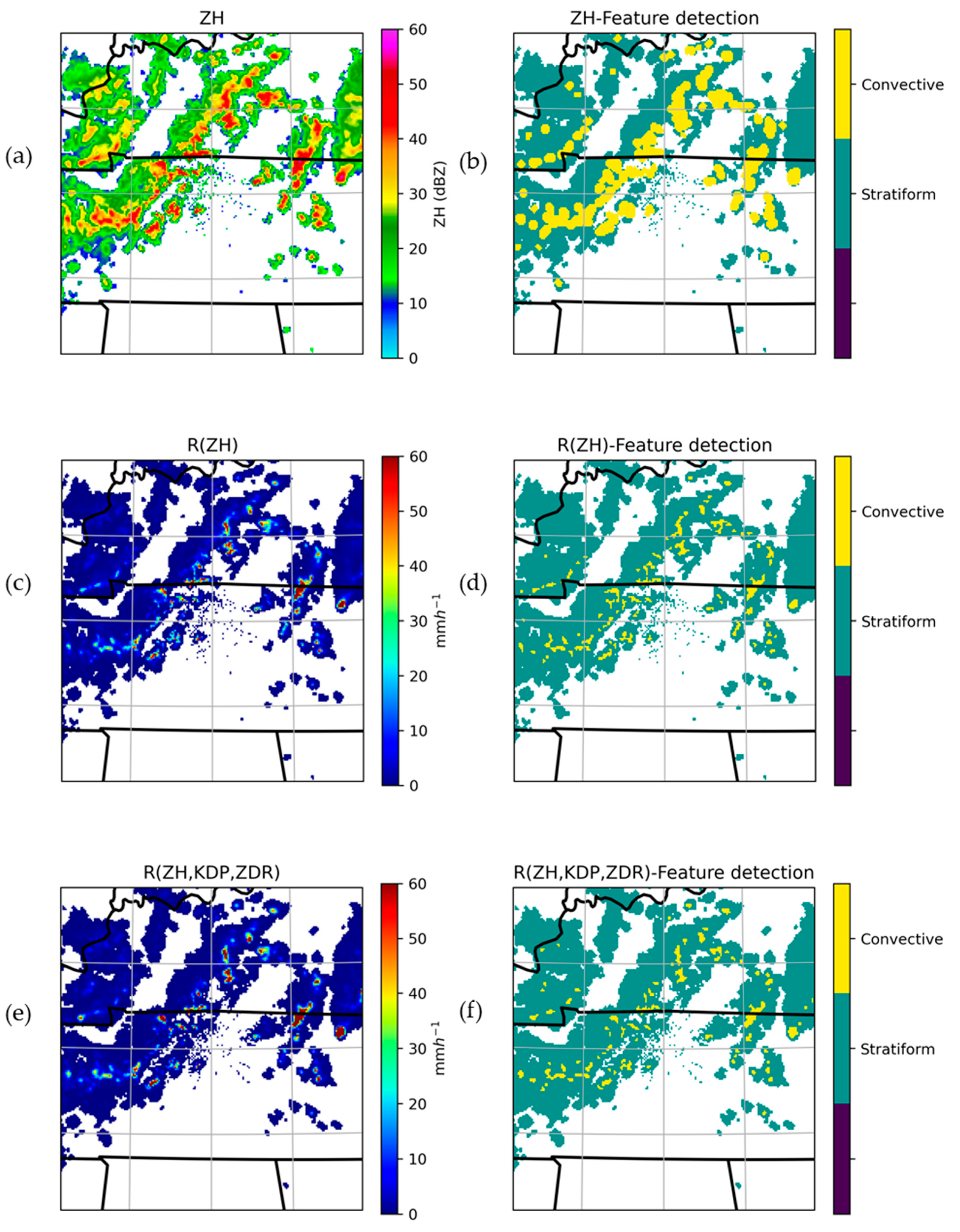
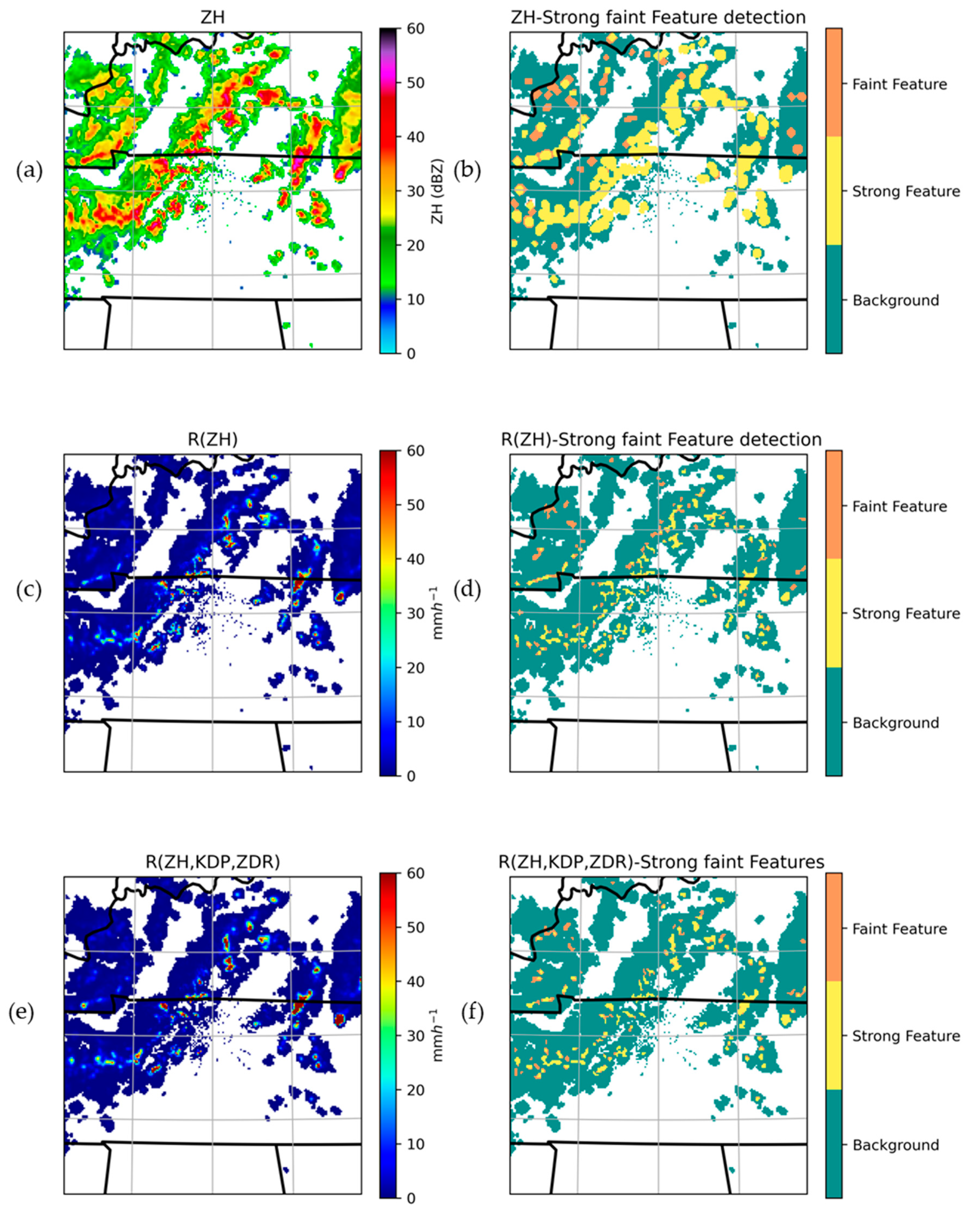
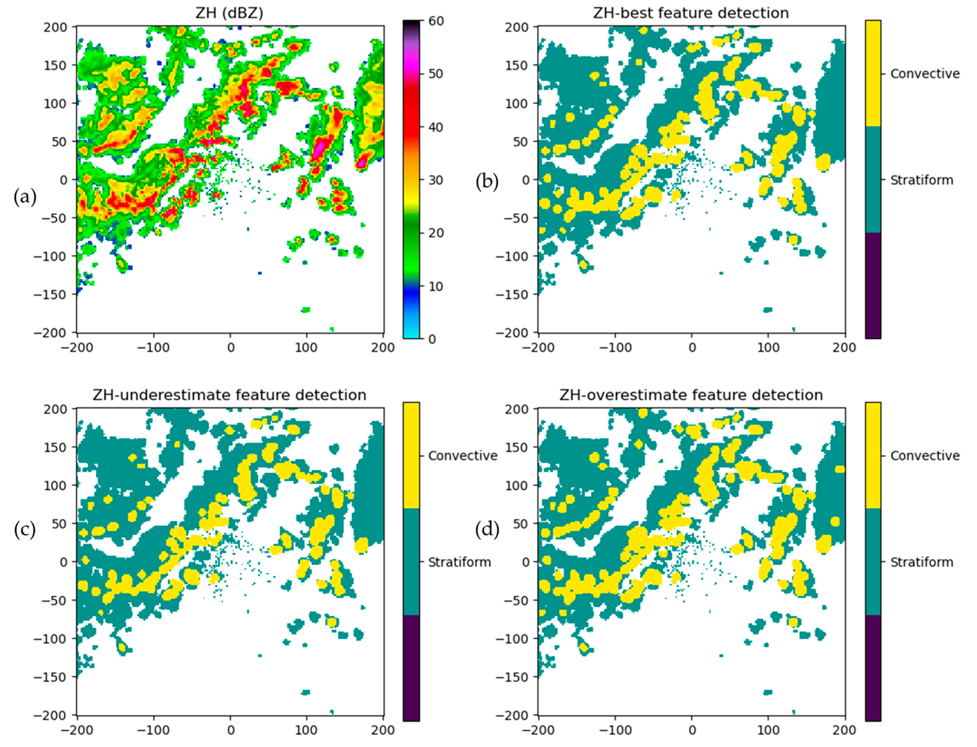
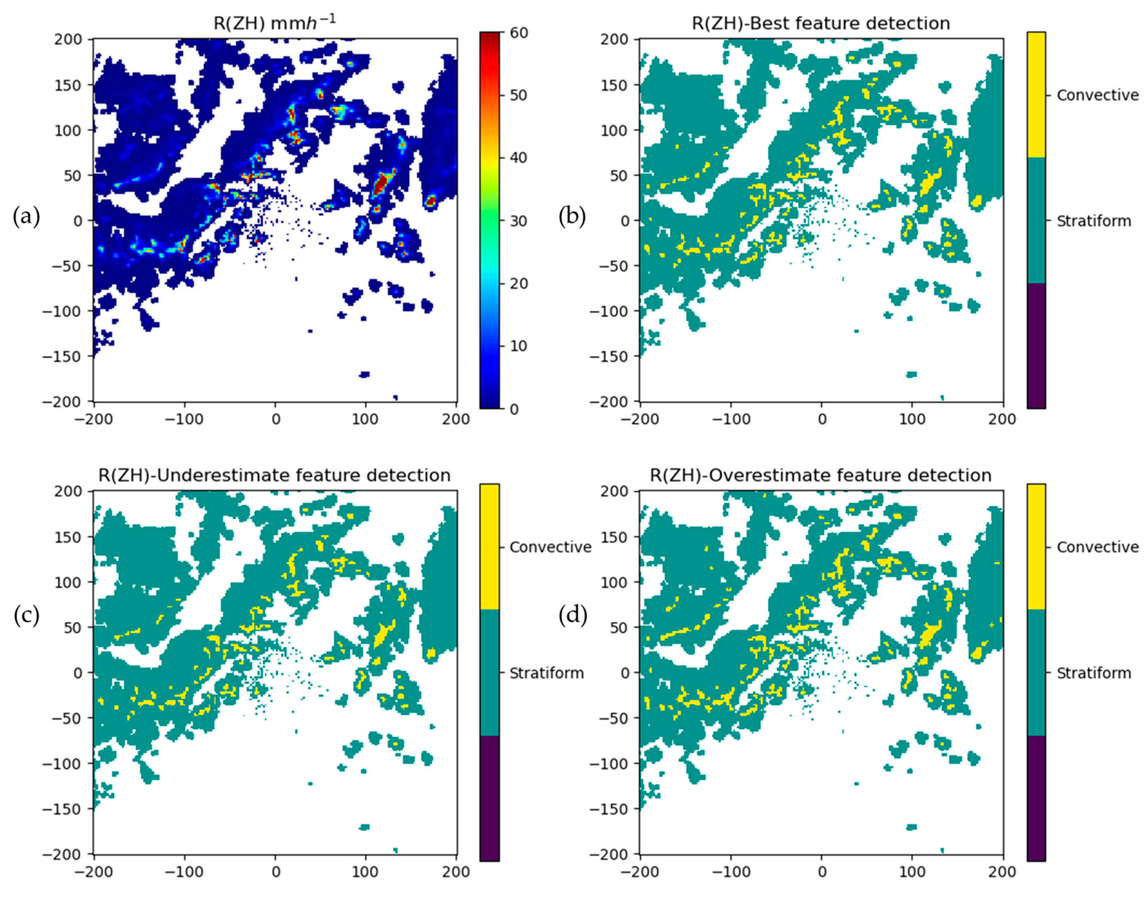
3.4. The Results of Feature Detection During the Event
4. Discussion
5. Conclusions
Author Contributions
Funding
Data Availability Statement
Acknowledgments
Conflicts of Interest
References
- Ghada, W.; Casellas, E.; Herbinger, J.; Garcia-Benadí, A.; Bothmann, L.; Estrella, N.; Bech, J.; Menzel, A. Stratiform and Convective Rain Classification Using Machine Learning Models and Micro Rain Radar. Remote Sens. 2022, 14, 4563. [Google Scholar] [CrossRef]
- Tomkins, L.M.; Yuter, S.E.; Miller, M.A. Dual Adaptive Differential Threshold Method for Automated Detection of Faint and Strong Echo Features in Radar Observations of Winter Storms. Atmos. Meas. Tech. 2024, 17, 3377–3399. [Google Scholar] [CrossRef]
- Yang, Z.; Liu, P.; Yang, Y. Convective/Stratiform Precipitation Classification Using Ground-Based Doppler Radar Data Based on the K-Nearest Neighbor Algorithm. Remote Sens. 2019, 11, 2277. [Google Scholar] [CrossRef]
- Vasiloff, S.V.; Seo, D.J.; Howard, K.W.; Zhang, J.; Kitzmiller, D.H.; Mullusky, M.G.; Krajewski, W.F.; Brandes, E.A.; Rabin, R.M.; Berkowitz, D.S.; et al. Improving QPE and Very Short Term QPF: An Initiative for a Community-Wide Integrated Approach. Bull. Am. Meteorol. Soc. 2007, 88, 1899–1911. [Google Scholar] [CrossRef]
- Gu, J.Y.; Ryzhkov, A.; Zhang, P.; Neilley, P.; Knight, M.; Wolf, B.; Lee, D.I. Polarimetric Attenuation Correction in Heavy Rain at C Band. J. Appl. Meteorol. Climatol. 2011, 50, 39–58. [Google Scholar] [CrossRef]
- Zhang, J.; Tang, L.; Cocks, S.; Zhang, P.; Ryzhkov, A.; Howard, K.; Langston, C.; Kaney, B. A Dual-Polarization Radar Synthetic QPE for Operations. J. Hydrometeorol. 2020, 21, 2507–2521. [Google Scholar] [CrossRef]
- Biggerstaff, M.I.; Listema, S.A. An Improved Scheme for Convective/Stratiform Echo Classification Using Radar Reflectivity. J. Appl. Meteorol. 2000, 39, 2129–2150. [Google Scholar] [CrossRef]
- Yuter, S.E.; Houze, R.A.; Smith, E.A.; Wilheit, T.T.; Zipser, E. Physical Characterization of Tropical Oceanic Convection Observed in KWAJEX. J. Appl. Meteorol. 2005, 44, 385–415. [Google Scholar] [CrossRef]
- Kumjian, M.R.; Prat, O.P.; Reimel, K.J.; van Lier-Walqui, M.; Morrison, H.C. Dual-Polarization Radar Fingerprints of Precipitation Physics: A Review. Remote Sens. 2022, 14, 3706. [Google Scholar] [CrossRef]
- Ribaud, J.F.; Augusto Toledo MacHado, L.; Biscaro, T. X-Band Dual-Polarization Radar-Based Hydrometeor Classification for Brazilian Tropical Precipitation Systems. Atmos. Meas. Tech. 2019, 12, 811–837. [Google Scholar] [CrossRef]
- Ryzhkov, A.; Giangrande, S.; Schuur, T. Rainfall Measurements with the Polarimetric WSR-88D Radar. Data Process. 2003, 98, 502–515. [Google Scholar]
- Ryzhkov, A.V.; Schuur, T.J.; Burgess, D.W.; Heinselman, P.L.; Giangrande, S.E.; Zrnic, D.S. The Joint Polarization Experiment: Polarimetric Rainfall Measurements and Hydrometeor Classification. Bull. Am. Meteorol. Soc. 2005, 86, 809–824. [Google Scholar] [CrossRef]
- Ryzhkov, A.V.; Giangrande, S.; Schuur, T.J. Rainfall Estimation with a Polarimetric Prototype of the Operational Wsr-88D Radar. 31st Conf. Radar Meteorol. 2003, 44, 208–211. [Google Scholar]
- Stepanian, P.M.; Horton, K.G.; Melnikov, V.M.; Zrnić, D.S.; Gauthreaux, S.A. Dual-Polarization Radar Products for Biological Applications. Ecosphere 2016, 7, e01539. [Google Scholar] [CrossRef]
- Walsh, T.H.; Lansford, J.W.; Hromadka, T.V.; Rao, P. Dual-Polarization Radar Rainfall Prediction and Rain Gauge Data. BMC Res. Notes 2021, 14, 1–3. [Google Scholar] [CrossRef]
- Guo, Z.; Hu, S.; Zeng, G.; Chen, X.; Zhang, H.; Xia, F.; Zhuang, J.; Chen, M.; Fan, Y. An Improved S-Band Polarimetric Radar-Based QPE Algorithm for Typhoons over South China Using 2DVD Observations. Atmosphere 2023, 14, 935. [Google Scholar] [CrossRef]
- Ryu, S.; Song, J.J. Radar–Rain Gauge Merging for High-Spatiotemporal-Resolution Rainfall Estimation Using Radial Basis Function Interpolation. Remote Sens. 2025, 17, 530. [Google Scholar] [CrossRef]
- Anagnostou, E.N. A Convective/Stratiform Precipitation Classification Algorithm for Volume Scanning Weather Radar Observations. Meteorol. Appl. 2004, 11, 291–300. [Google Scholar] [CrossRef]
- Steiner, M.; Houze, R.A.; Yuter, S.E. Climatological Characterization of Three-Dimensional Storm Structure from Operational Radar and Rain Gauge Data. J. Appl. Meteorol. 1995, 34, 1978–2007. [Google Scholar] [CrossRef]
- Yuter, S.E.; Houze, R.A. Measurements of Raindrop Size Distributions over the Pacific Warm Pool and Implications for Z-R Relations. J. Appl. Meteorol. 1997, 36, 847–867. [Google Scholar] [CrossRef]
- Huber, M.; Trapp, J. A Review of NEXRAD Level II: Data, Distribution, and Applications. J. Terr. Obs. 2009, 1, 5–15. [Google Scholar]
- Park, H.S.; Ryzhkov, A.V.; Zrnić, D.S.; Kim, K.E. The Hydrometeor Classification Algorithm for the Polarimetric WSR-88D: Description and Application to an MCS. Weather Forecast. 2009, 24, 730–748. [Google Scholar] [CrossRef]
- Binetti, M.S.; Campanale, C.; Massarelli, C.; Uricchio, V.F. The Use of Weather Radar Data: Possibilities, Challenges and Advanced Applications. Earth 2022, 3, 157–171. [Google Scholar] [CrossRef]
- Hu, S.M.; Huang, X.Y.; Ma, Y.R. Turbulence and Rainfall Microphysical Parameters Retrieval and Their Relationship Analysis Based on Wind Profiler Radar Data. J. Trop. Meteorol. 2021, 27, 291–302. [Google Scholar] [CrossRef]
- Vulpiani, G.; Montopoli, M.; Passeri, L.D.; Gioia, A.G.; Giordano, P.; Marzano, F.S. On the Use of Dual-Polarized c-Band Radar for Operational Rainfall Retrieval in Mountainous Areas. J. Appl. Meteorol. Climatol. 2012, 51, 405–425. [Google Scholar] [CrossRef]
- Zhang, S.; Huang, X.; Min, J.; Chu, Z.; Zhuang, X.; Zhang, H. Improved Fuzzy Logic Method to Distinguish between Meteorological and Non-Meteorological Echoes Using C-Band Polarimetric Radar Data. Atmos. Meas. Tech. 2020, 13, 537–551. [Google Scholar] [CrossRef]
- Lakshmanan, V.; Karstens, C.; Krause, J.; Tang, L. Quality Control of Weather Radar Data Using Polarimetric Variables. J. Atmos. Ocean. Technol. 2014, 31, 1234–1249. [Google Scholar] [CrossRef]
- Ośródka, K.; Szturc, J. Improvement in Algorithms for Quality Control of Weather Radar Data (RADVOL-QC System). Atmos. Meas. Tech. 2022, 15, 261–277. [Google Scholar] [CrossRef]
- Michelson, D.; Hansen, B.; Jacques, D.; Lemay, F.; Rodriguez, P. Monitoring the Impacts of Weather Radar Data Quality Control for Quantitative Application at the Continental Scale. Meteorol. Appl. 2020, 27, 1–12. [Google Scholar] [CrossRef]
- Helmus, J.J.; Collis, S.M. The Python ARM Radar Toolkit (Py-ART), a Library for Working with Weather Radar Data in the Python Programming Language. J. Open Res. Softw. 2016, 4, 25. [Google Scholar] [CrossRef]
- Island, W.; Heistermann, M. The Emergence of Open-Source Software for the Weather Radar Community. Bull. Am. Meteorol. Soc. 2015, 96, 117–128. [Google Scholar] [CrossRef]
- Kumjian, M.R. Principles and Applications of Dual-Polarization Weather Radar. Part II: Warm- and Cold-Season Applications. J. Oper. Meteorol. 2013, 1, 226–242. [Google Scholar] [CrossRef]
- Montopoli, M.; Roberto, N.; Adirosi, E.; Gorgucci, E.; Baldini, L. Investigation of Weather Radar Quantitative Precipitation Estimation Methodologies in Complex Orography. Atmosphere 2017, 8, 34. [Google Scholar] [CrossRef]


| Coefficients | QPE Retrieval Formulas | Coefficient Values | Reference |
|---|---|---|---|
| az;bz | [12] | ||
| akdp;bKDP | [12] | ||
| aDR;bDR;cDR | [13] | ||
| aDP;bDP;cDP | [13] |
| Parameters | Reflectivity | Rainfall Rate (QPE) |
|---|---|---|
| dB_averaging | True | False |
| always_core_thres | 40 dBZ | 25 mmh−1 |
| bkg_rad_km | 6 km | 6 km |
| calc_thres | 0.75 | 0.75 |
| use_cosine | True | True |
| max_diff | 5 dBZ | 2.5 mmh−1 |
| zero_diff_cos_val | 55 dBZ | 13 mmh−1 |
| weak_echo_thres | 10 dBZ | 0.5 mmh−1 |
| estimate_flag | True | True |
Disclaimer/Publisher’s Note: The statements, opinions and data contained in all publications are solely those of the individual author(s) and contributor(s) and not of MDPI and/or the editor(s). MDPI and/or the editor(s) disclaim responsibility for any injury to people or property resulting from any ideas, methods, instructions or products referred to in the content. |
© 2025 by the authors. Licensee MDPI, Basel, Switzerland. This article is an open access article distributed under the terms and conditions of the Creative Commons Attribution (CC BY) license (https://creativecommons.org/licenses/by/4.0/).
Share and Cite
Mikidadi, N.D.; Huang, X.; Bu, L. The Application of the Convective–Stratiform Classification Algorithm for Feature Detection in Polarimetric Radar Variables and QPE Retrieval During Warm-Season Convection. Remote Sens. 2025, 17, 1176. https://doi.org/10.3390/rs17071176
Mikidadi ND, Huang X, Bu L. The Application of the Convective–Stratiform Classification Algorithm for Feature Detection in Polarimetric Radar Variables and QPE Retrieval During Warm-Season Convection. Remote Sensing. 2025; 17(7):1176. https://doi.org/10.3390/rs17071176
Chicago/Turabian StyleMikidadi, Ndabagenga Daudi, Xingyou Huang, and Lingbing Bu. 2025. "The Application of the Convective–Stratiform Classification Algorithm for Feature Detection in Polarimetric Radar Variables and QPE Retrieval During Warm-Season Convection" Remote Sensing 17, no. 7: 1176. https://doi.org/10.3390/rs17071176
APA StyleMikidadi, N. D., Huang, X., & Bu, L. (2025). The Application of the Convective–Stratiform Classification Algorithm for Feature Detection in Polarimetric Radar Variables and QPE Retrieval During Warm-Season Convection. Remote Sensing, 17(7), 1176. https://doi.org/10.3390/rs17071176