


Insights into the Interconnected Dynamics of Groundwater Drought and InSAR-Derived Subsidence in the Marand Plain, Northwestern Iran


Abstract
1. Introduction
2. Materials and Methods
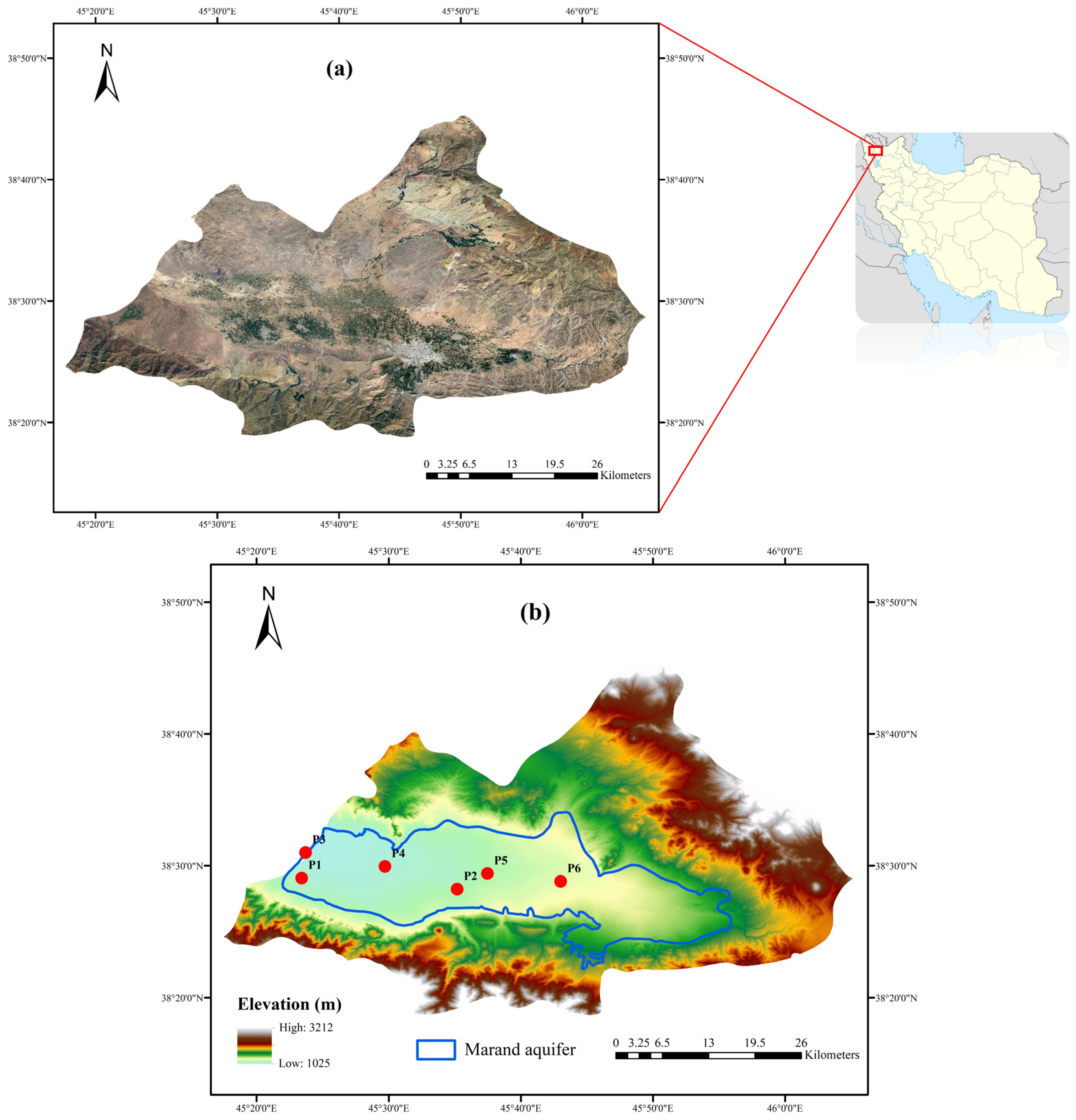
2.1. Study Area
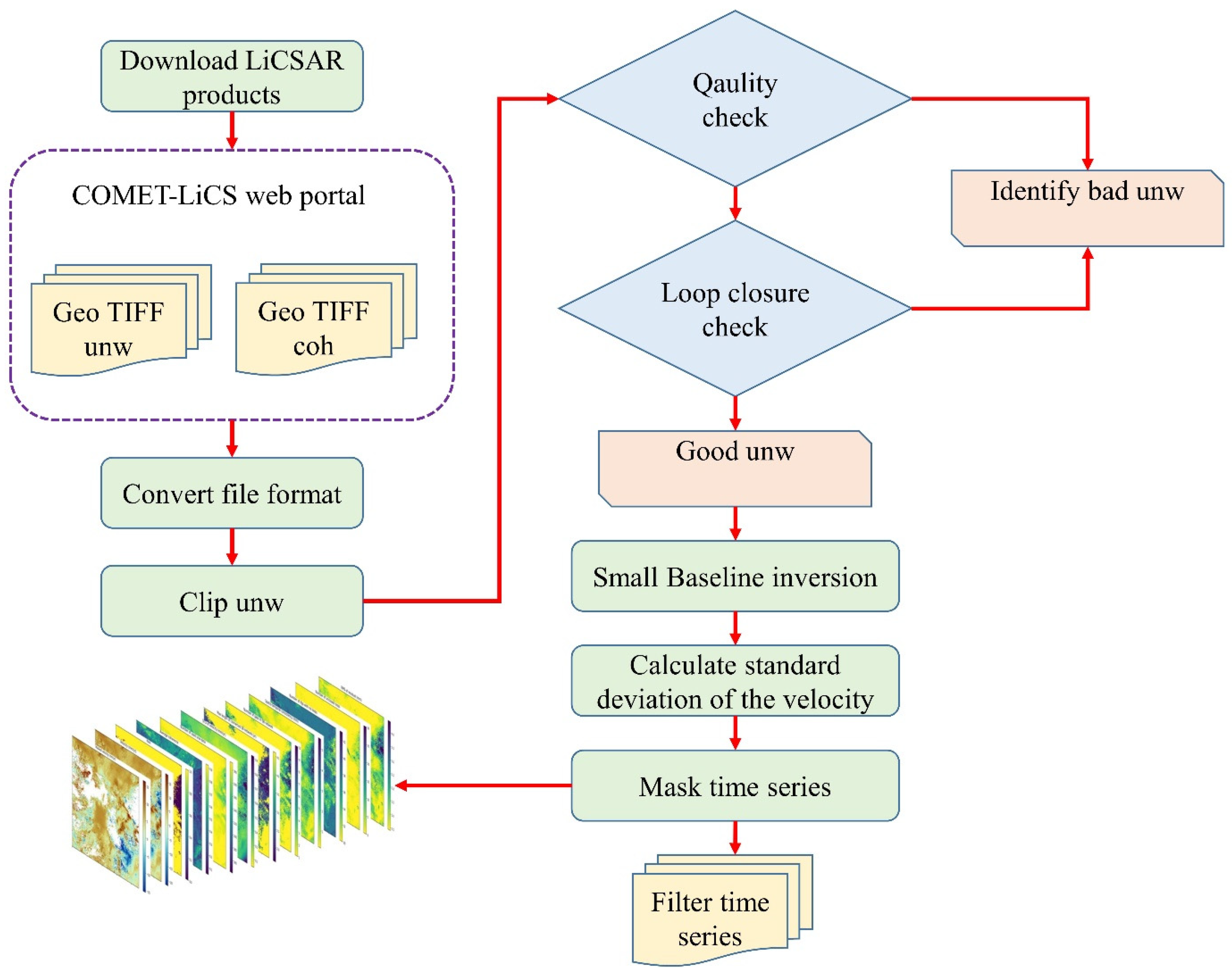
2.2. InSAR Data
2.3. Standardized Groundwater Index
2.4. Probability Density Functions
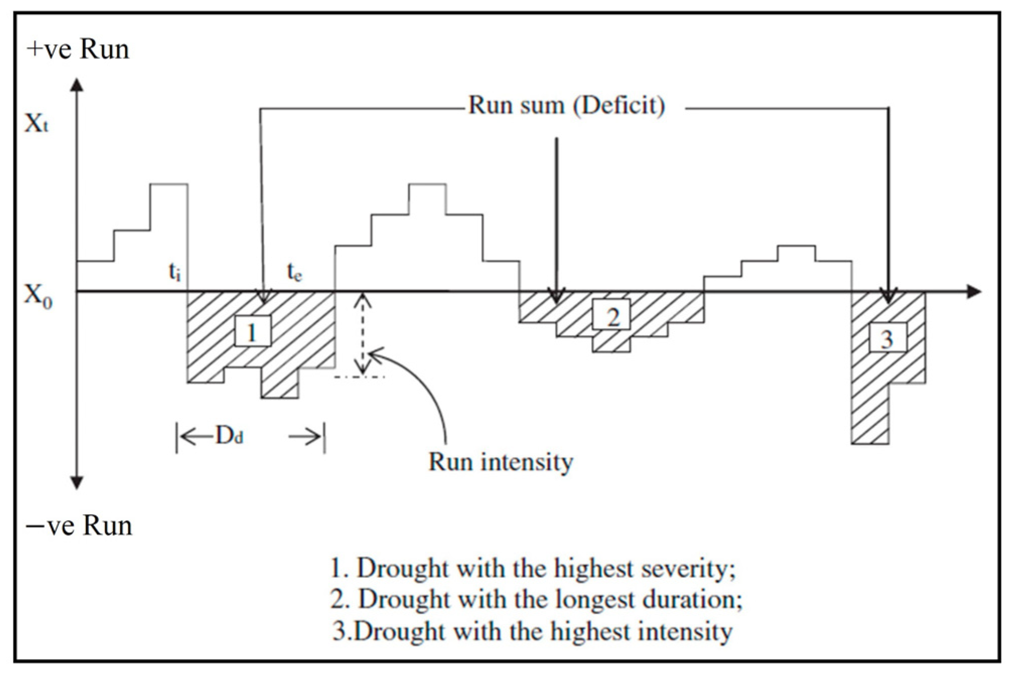
2.5. Drought Characteristics
2.6. Nonparametric Mann–Kendall Test
2.7. Trend-Free Pre-Whitening (TFPW) Mann–Kendall Test
- (1)
- Calculate the linear trend (β) for each index series, Xt (where t = 1, 2,…, N):
- (2)
- Generate a new series, Yt, by eliminating the trend component from the original series:
- (3)
- Calculate the first-order autocorrelation coefficient, r, for the new series Yt, and conduct a significance test on r with a significance level of 0.1. If the test is significant, proceed by applying the MK method directly to test the original series, Xt. If the test is not significant, proceed to step (4) for further preprocessing.
- (4)
- Create a new series, , by eliminating the autocorrelation terms from the original series. Then, reintroduce the trend component to form a new series, , which is free from the influence of autocorrelation interference:
- (5)
- Substitute the new series, , into the MK test.
2.8. Continuous Wavelet Transform (CWT)
2.9. Wavelet Transform Coherence (WTC)
3. Results
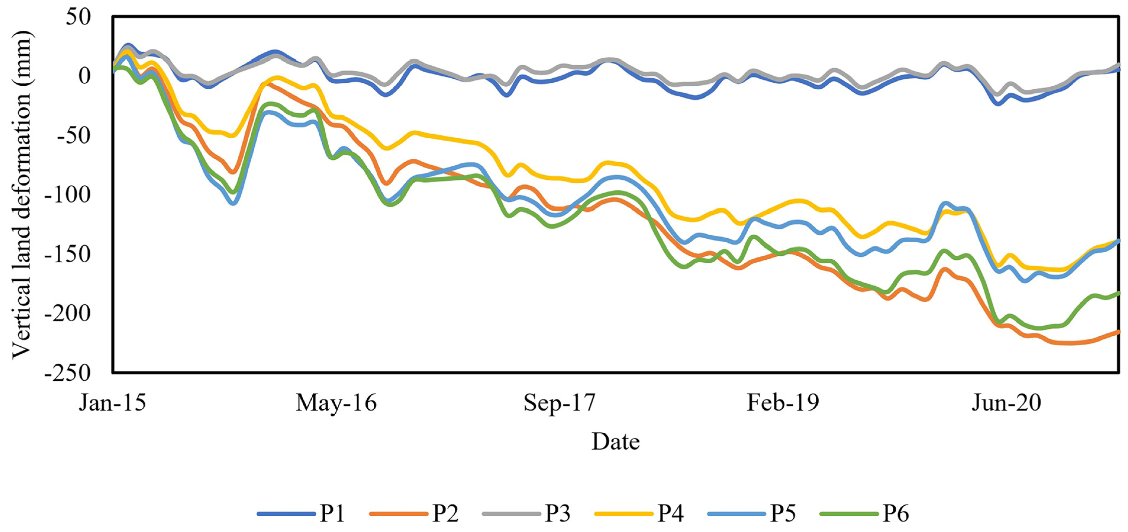
3.1. Long-Term Deformation Rates
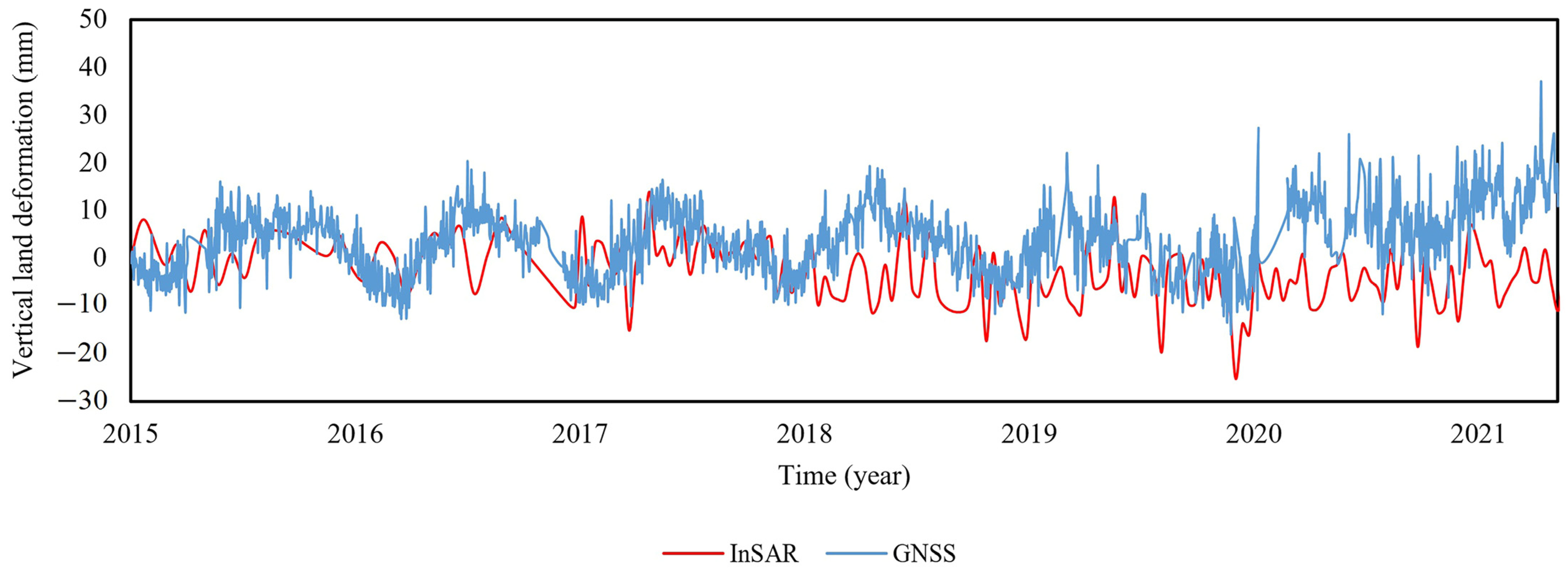
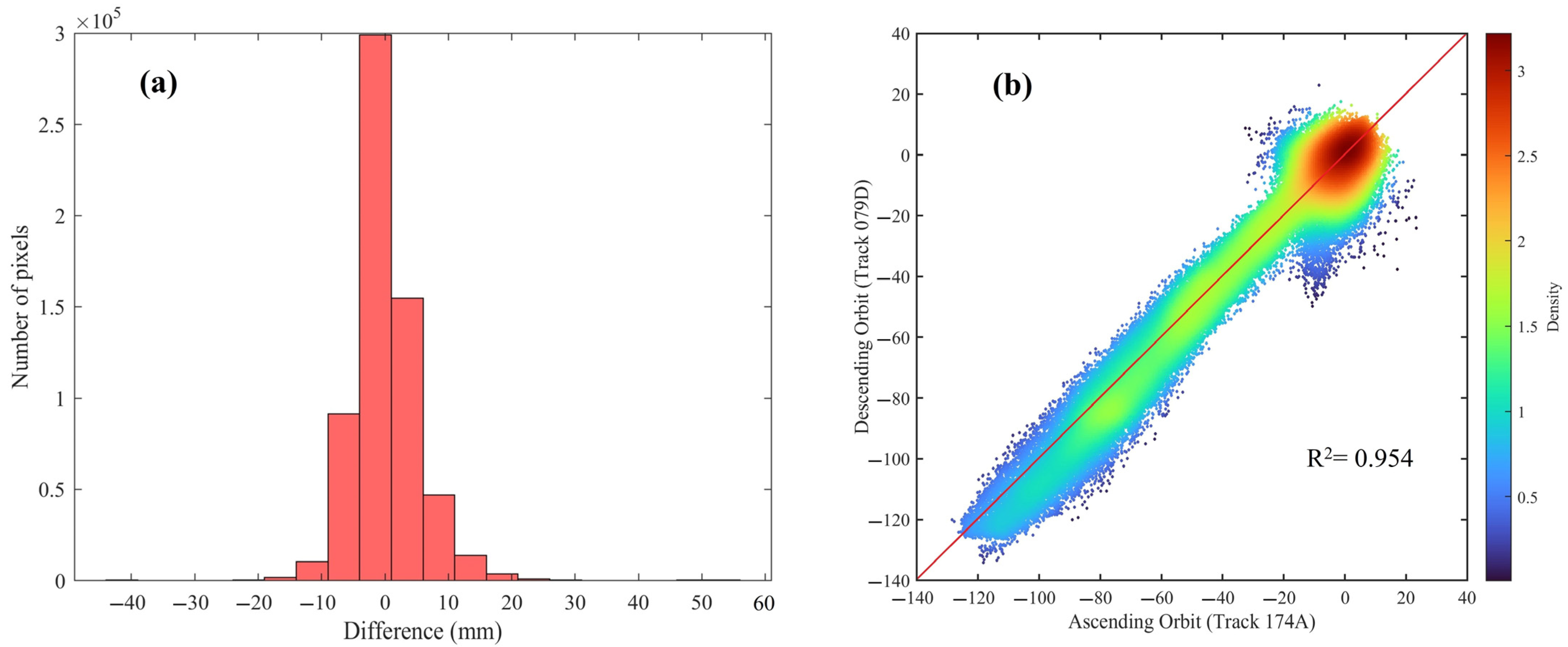
3.2. InSAR Validation
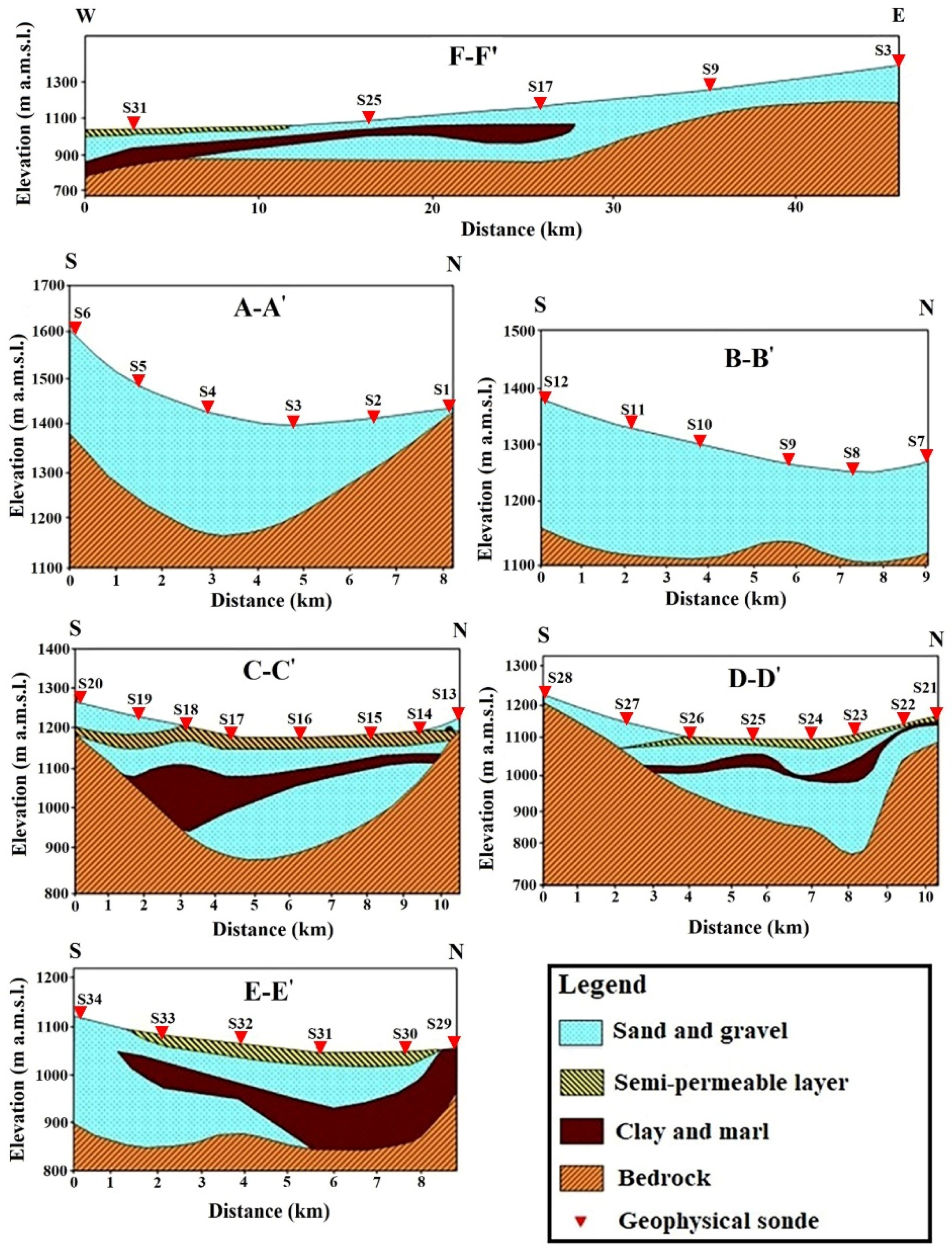
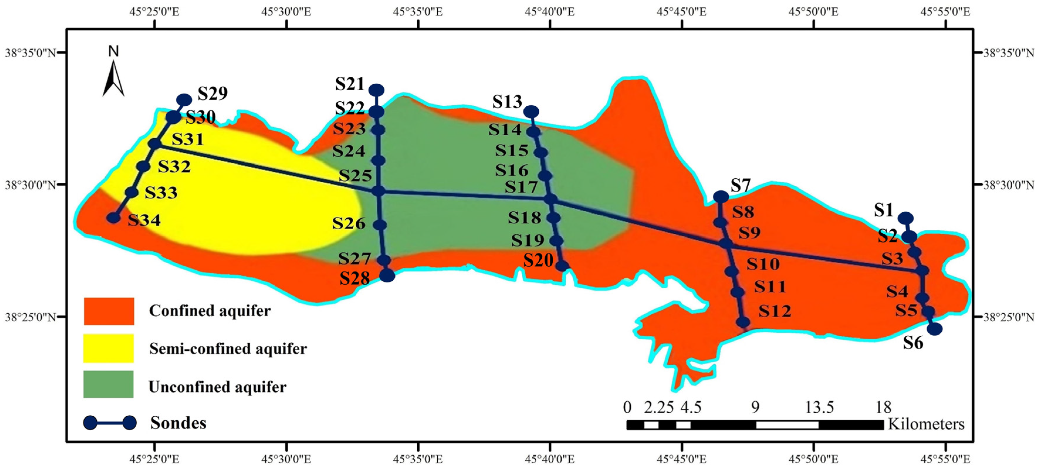
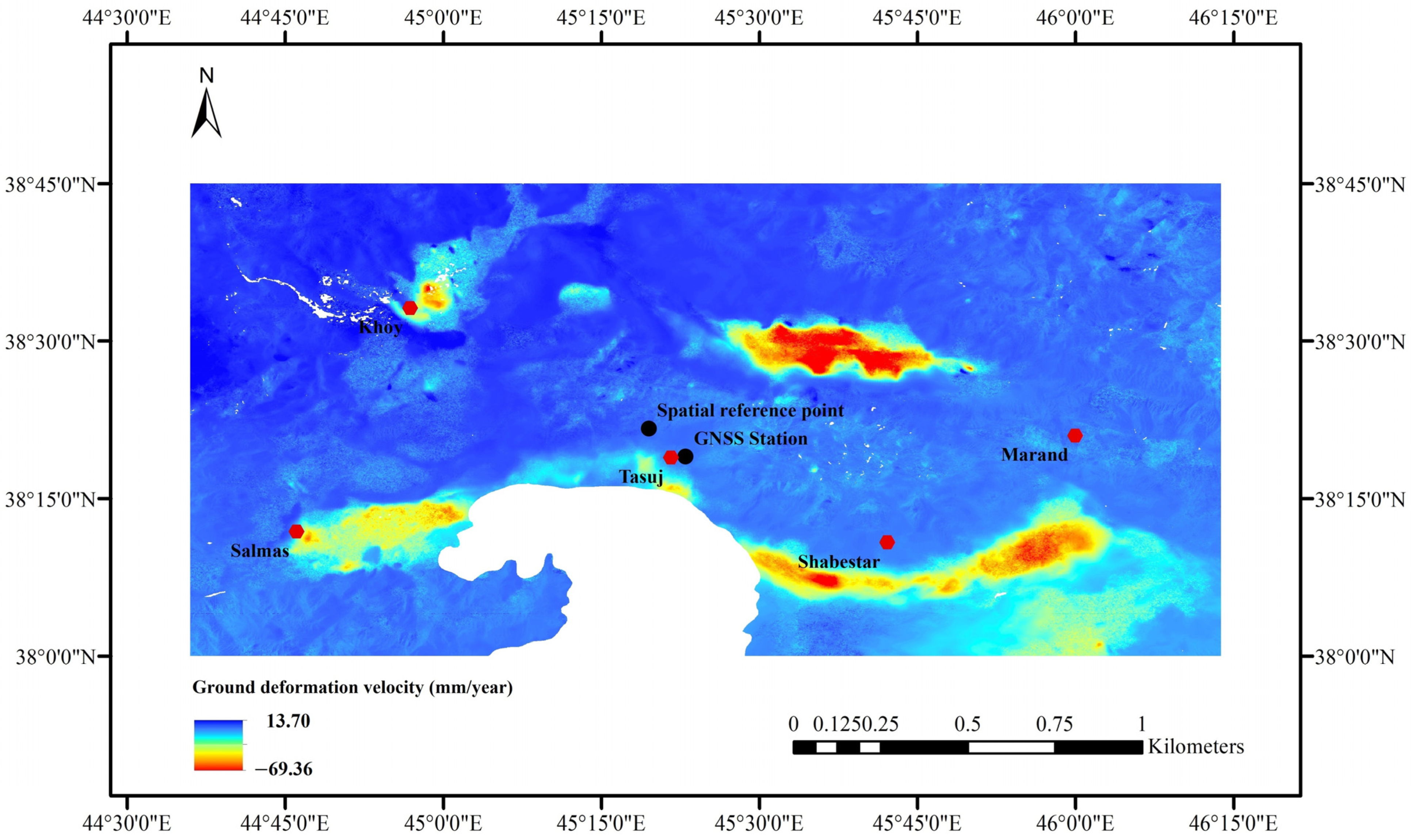
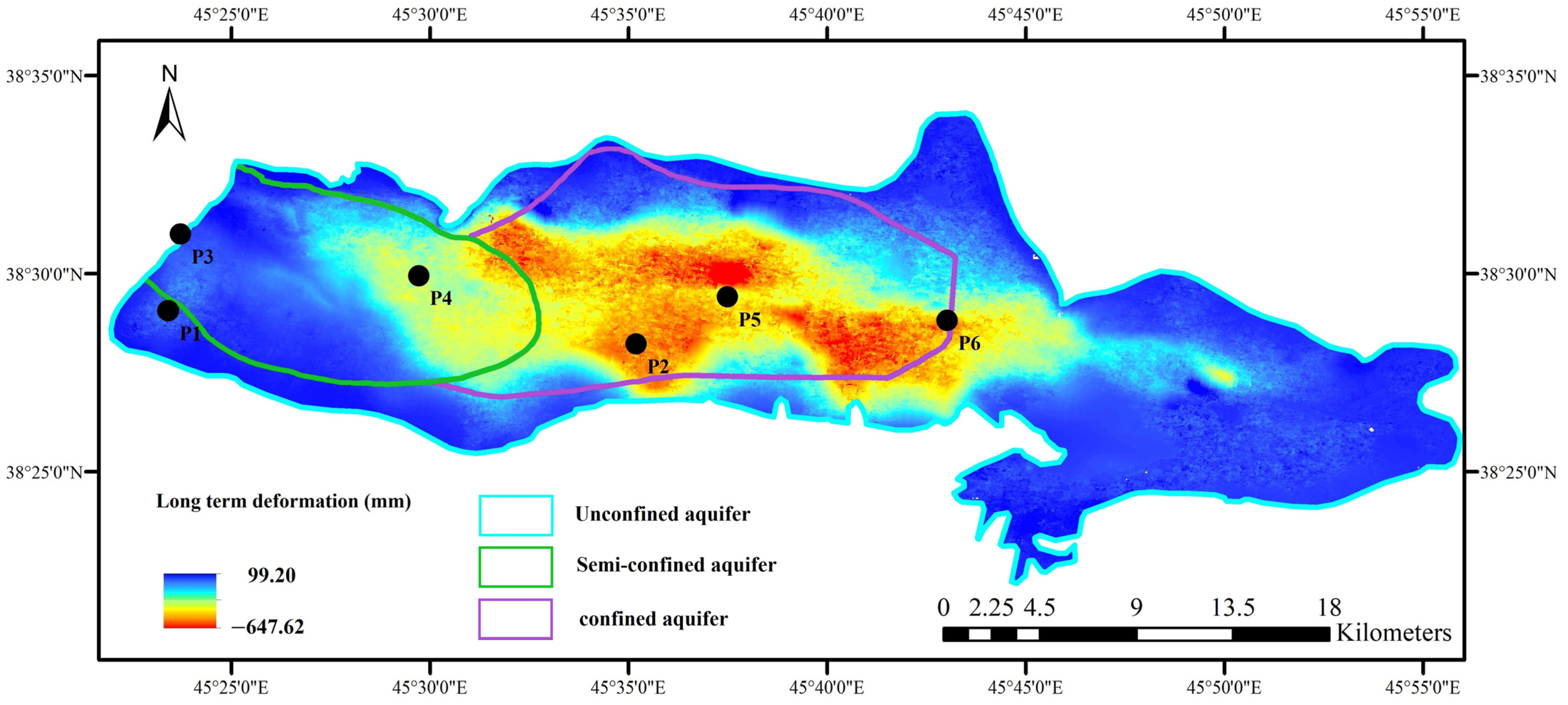
3.3. Subsidence Map of the Marand Aquifer
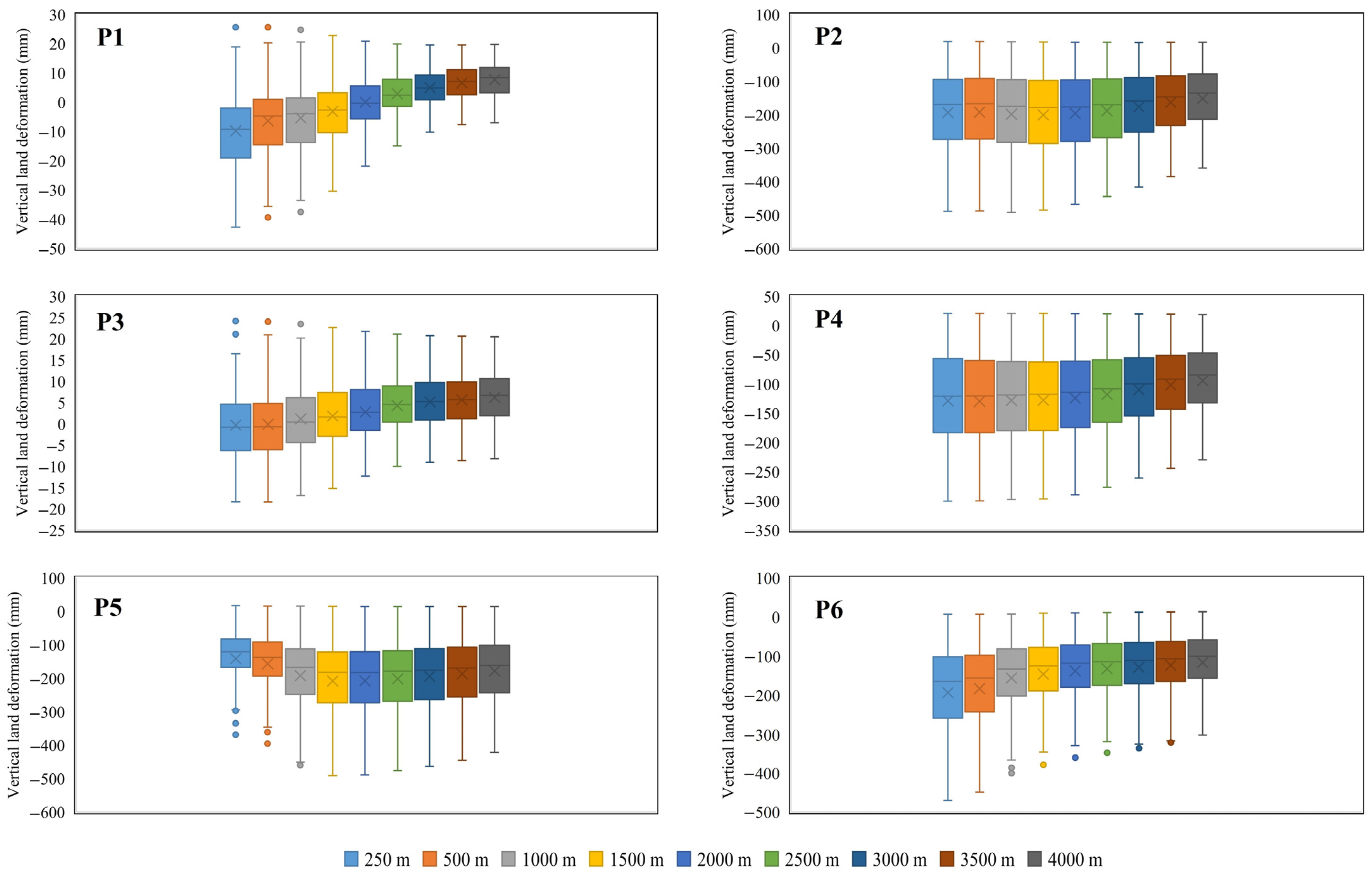
3.4. Identification of Critical Impact Zone
3.5. Trend Analysis of Groundwater Drought
3.6. Groundwater Drought Monitoring
3.7. Relationship Between Groundwater Drought and Land Subsidence
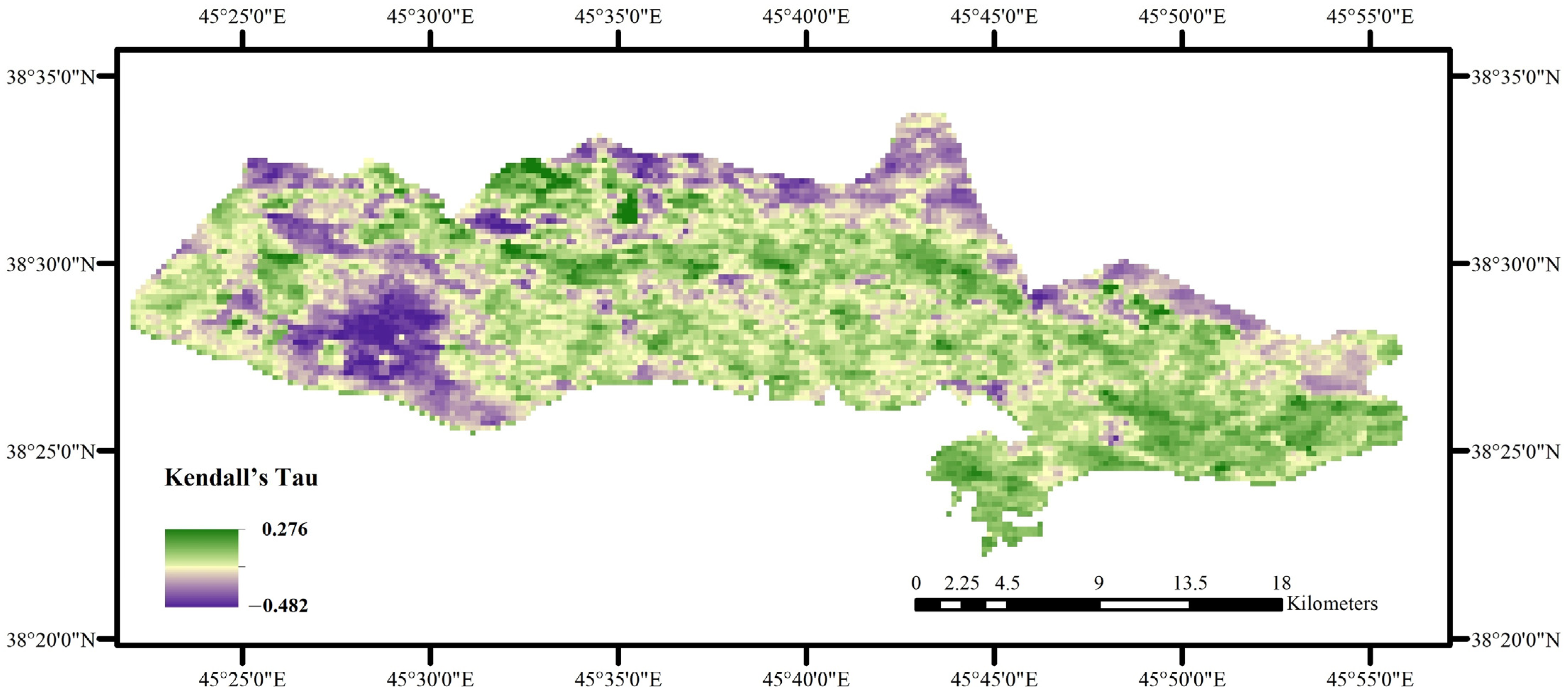
3.8. Correlation Analysis
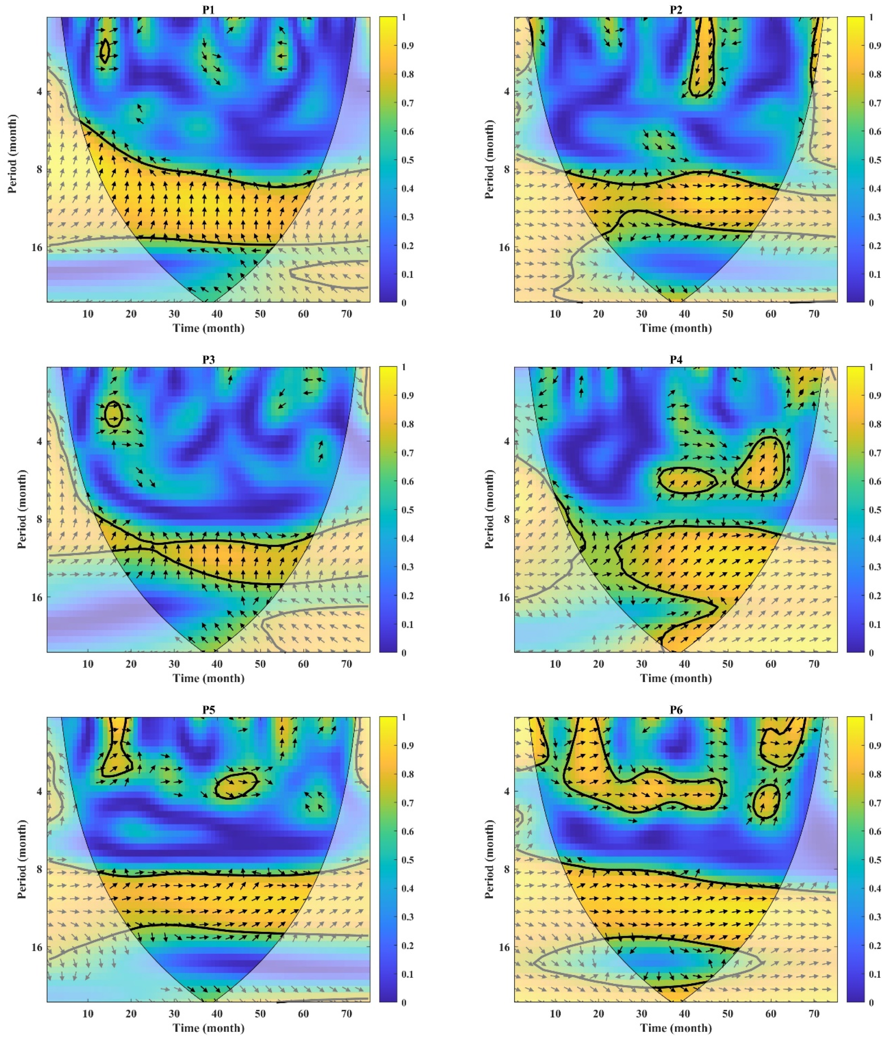
3.9. Wavelet Coherence Analysis
4. Discussion
5. Conclusions
Supplementary Materials
Author Contributions
Funding
Data Availability Statement
Conflicts of Interest
References
- Sheffield, J.; Andreadis, K.M.; Wood, E.F.; Lettenmaier, D.P. Global and continental drought in the second half of the twentieth century: Severity–area–duration analysis and temporal variability of large-scale events. J. Clim. 2009, 22, 1962–1981. [Google Scholar]
- Nafarzadegan, A.R.; Zadeh, M.R.; Kherad, M.; Ahani, H.; Gharehkhani, A.; Karampoor, M.A.; Kousari, M.R. Drought area monitoring during the past three decades in Fars province, Iran. Quat. Int. 2012, 250, 27–36. [Google Scholar]
- Mishra, A.K.; Singh, V.P. A review of drought concepts. J. Hydrol. 2010, 391, 202–216. [Google Scholar]
- Bloomfield, J.P.; Marchant, B.P.; Bricker, S.H.; Morgan, R.B. Regional analysis of groundwater droughts using hydrograph classification. Hydrol. Earth Syst. Sci. 2015, 19, 4327–4344. [Google Scholar]
- Van Lanen, H.A.; Peters, E. Definition, effects and assessment of groundwater droughts. In Drought and Drought Mitigation in Europe; Springer: Dordrecht, The Netherlands, 2000; pp. 49–61. [Google Scholar]
- Bloomfield, J.P.; Marchant, B.P.; McKenzie, A.A. Changes in groundwater drought associated with anthropogenic warming. Hydrol. Earth Syst. Sci. 2019, 23, 1393–1408. [Google Scholar]
- Shahnazi, S.; Roushangar, K.; Hashemi, H. A novel implementation of pre-processing approaches and hybrid kernel-based model for short-and long-term groundwater drought forecasting. J. Hydrol. 2025, 652, 132667. [Google Scholar]
- Ren, X.; Li, P.; Wang, D.; Zhang, Q.; Ning, J. Drivers and characteristics of groundwater drought under human interventions in arid and semiarid areas of China. J. Hydrol. 2024, 631, 130839. [Google Scholar]
- Xu, Y.; Yang, Y.; Chen, X.; Liu, Y. Bibliometric analysis of global NDVI research trends from 1985 to 2021. Remote Sens. 2022, 14, 3967. [Google Scholar] [CrossRef]
- Mousavi, S.M.; Shamsai, A.; Naggar, M.H.E.; Khamehchian, M. A GPS-based monitoring program of land subsidence due to groundwater withdrawal in Iran. Can. J. Civ. Eng. 2001, 28, 452–464. [Google Scholar]
- Abidin, H.Z.; Andreas, H.; Gamal, M.; Djaja, R.; Subarya, C.; Hirose, K.; Maruyama, Y.; Murdohardono, D.; Rajiyowiryono, H. Monitoring land subsidence of Jakarta (Indonesia) using leveling, GPS survey and InSAR techniques. In A Window on the Future of Geodesy, Proceedings of the International Association of Geodesy IAG General Assembly, Sapporo, Japan, 30 June–11 July 2003; Springer: Berlin/Heidelberg, Germany, 2005; pp. 561–566. [Google Scholar]
- Dehkordi, A.T.; Hashemi, H.; Naghibi, A.; Mehran, A. Ensemble of pruned bagged mixture density networks for improved water quality retrieval using Sentinel-2 and Landsat-8 remote sensing data. IEEE Geosci. Remote Sens. Lett. 2024, 21, 1504705. [Google Scholar]
- Dehkordi, A.T.; Zoej, M.J.V.; Mehran, A.; Jafari, M.; Chegoonian, A.M. Fuzzy similarity analysis of effective training samples to improve machine learning estimations of water quality parameters using Sentinel-2 remote sensing data. IEEE J. Sel. Top. Appl. Earth Obs. Remote Sens. 2024, 17, 5121–5136. [Google Scholar]
- Li, S.; Xu, W.; Li, Z. Review of the SBAS InSAR Time-series algorithms, applications, and challenges. Geod. Geodyn. 2022, 13, 114–126. [Google Scholar]
- Famiglietti, J.S. The global groundwater crisis. Nat. Clim. Chang. 2014, 4, 945–948. [Google Scholar]
- Smith, R.; Knight, R. Modeling land subsidence using InSAR and airborne electromagnetic data. Water Resour. Res. 2019, 55, 2801–2819. [Google Scholar]
- Miller, M.M.; Jones, C.E.; Sangha, S.S.; Bekaert, D.P. Rapid drought-induced land subsidence and its impact on the California aqueduct. Remote Sens. Environ. 2020, 251, 112063. [Google Scholar]
- Barthelemy, S.; Bonan, B.; Calvet, J.C.; Grandjean, G.; Moncoulon, D.; Kapsambelis, D.; Bernardie, S. A new approach for drought index adjustment to clay-shrinkage-induced subsidence over France: Advantages of the interactive leaf area index. Nat. Hazards Earth Syst. Sci. 2024, 24, 999–1016. [Google Scholar]
- Ghorbani, Z.; Khosravi, A.; Maghsoudi, Y.; Mojtahedi, F.F.; Javadnia, E.; Nazari, A. Use of InSAR data for measuring land subsidence induced by groundwater withdrawal and climate change in Ardabil Plain, Iran. Sci. Rep. 2022, 12, 13998. [Google Scholar]
- Welch, J.; Wang, G.; Bao, Y.; Zhang, S.; Huang, G.; Hu, X. Unveiling the hidden threat: Drought-induced inelastic subsidence in expansive soils. Geophys. Res. Lett. 2024, 51, e2023GL107549. [Google Scholar]
- Chen, M.; Tomás, R.; Li, Z.; Motagh, M.; Li, T.; Hu, L.; Gong, H.; Li, X.; Yu, J.; Gong, X. Imaging land subsidence induced by groundwater extraction in Beijing (China) using satellite radar interferometry. Remote Sens. 2016, 8, 468. [Google Scholar] [CrossRef]
- Meldebekova, G.; Yu, C.; Li, Z.; Song, C. Quantifying ground subsidence associated with aquifer overexploitation using space-borne radar interferometry in Kabul, Afghanistan. Remote Sens. 2020, 12, 2461. [Google Scholar] [CrossRef]
- Babaee, S.; Mousavi, Z.; Masoumi, Z.; Malekshah, A.H.; Roostaei, M.; Aflaki, M. Land subsidence from interferometric SAR and groundwater patterns in the Qazvin plain, Iran. Int. J. Remote Sens. 2020, 41, 4780–4798. [Google Scholar] [CrossRef]
- Gezgin, C. The influence of groundwater levels on land subsidence in Karaman (Turkey) using the PS-InSAR technique. Adv. Space Res. 2022, 70, 3568–3581. [Google Scholar] [CrossRef]
- Shahkarami, N. Temporal Analysis of Land Subsidence and Groundwater Depletion Using the DInSAR and Kriging Methods: A Case Study and Insights. J. Hydrol. Eng. 2024, 29, 04024011. [Google Scholar] [CrossRef]
- Farshbaf, A.; Mousavi, M.N.; Shahnazi, S. Vulnerability assessment of power transmission towers affected by land subsidence via interferometric synthetic aperture radar technique and finite element method analysis: A case study of Zanjan and Qazvin provinces. Environ. Dev. Sustain. 2024, 26, 10845–10864. [Google Scholar] [CrossRef]
- Bagheri-Gavkosh, M.; Hosseini, S.M.; Ataie-Ashtiani, B.; Sohani, Y.; Ebrahimian, H.; Morovat, F.; Ashrafi, S. Land subsidence: A global challenge. Sci. Total Environ. 2021, 778, 146193. [Google Scholar] [CrossRef] [PubMed]
- Bloomfield, J.P.; Marchant, B.P. Analysis of groundwater drought using a variant of the Standardised Precipitation Index. Hydrol. Earth Syst. Sci. Discuss. 2013, 10, 7537–7574. [Google Scholar]
- Gullacher, A.; Allen, D.M.; Goetz, J.D. Early warning indicators of groundwater drought in mountainous regions. Water Resour. Res. 2023, 59, e2022WR033399. [Google Scholar] [CrossRef]
- Andaryani, S.; Nourani, V.; Trolle, D.; Dehghani, M.; Asl, A.M. Assessment of land use and climate change effects on land subsidence using a hydrological model and radar technique. J. Hydrol. 2019, 578, 124070. [Google Scholar] [CrossRef]
- Fakhri, M.S.; Asghari Moghaddam, A.; Najib, M.; Barzegar, R. Investigation of nitrate concentrations in groundwater resources of Marand plain and groundwater vulnerability assessment using AVI and GODS methods. J. Environ. Stud. 2015, 41, 49–66. [Google Scholar]
- Hasan, M.F.; Smith, R.; Vajedian, S.; Pommerenke, R.; Majumdar, S. Global land subsidence mapping reveals widespread loss of aquifer storage capacity. Nat. Commun. 2023, 14, 6180. [Google Scholar] [CrossRef]
- Barzegar, R.; Moghaddam, A.A.; Tziritis, E.; Fakhri, M.S.; Soltani, S. Identification of hydrogeochemical processes and pollution sources of groundwater resources in the Marand plain, northwest of Iran. Environ. Earth Sci. 2017, 76, 297. [Google Scholar]
- Barzegar, R.; Moghaddam, A.A.; Deo, R.; Fijani, E.; Tziritis, E. Mapping groundwater contamination risk of multiple aquifers using multi-model ensemble of machine learning algorithms. Sci. Total Environ. 2018, 621, 697–712. [Google Scholar] [CrossRef]
- Lazecký, M.; Spaans, K.; González, P.J.; Maghsoudi, Y.; Morishita, Y.; Albino, F.; Elliott, J.; Greenall, N.; Hatton, E.; Hooper, A.; et al. LiCSAR: An automatic InSAR tool for measuring and monitoring tectonic and volcanic activity. Remote Sens. 2020, 12, 2430. [Google Scholar] [CrossRef]
- Morishita, Y.; Lazecky, M.; Wright, T.J.; Weiss, J.R.; Elliott, J.R.; Hooper, A. LiCSBAS: An open-source InSAR time series analysis package integrated with the LiCSAR automated Sentinel-1 InSAR processor. Remote Sens. 2020, 12, 424. [Google Scholar]
- Du, Q.; Chen, D.; Li, G.; Cao, Y.; Zhou, Y.; Chai, M.; Wang, F.; Qi, S.; Wu, G.; Gao, K.; et al. Preliminary Study on InSAR-Based Uplift or Subsidence Monitoring and Stability Evaluation of Ground Surface in the Permafrost Zone of the Qinghai–Tibet Engineering Corridor, China. Remote Sens. 2023, 15, 3728. [Google Scholar]
- Yu, C.; Li, Z.; Penna, N.T.; Crippa, P. Generic atmospheric correction model for interferometric synthetic aperture radar observations. J. Geophys. Res. Solid Earth 2018, 123, 9202–9222. [Google Scholar]
- Yeh, H.F. Spatiotemporal variation of the meteorological and groundwater droughts in central Taiwan. Front. Water 2021, 3, 636792. [Google Scholar]
- Haas, J.C.; Birk, S. Characterizing the spatiotemporal variability of groundwater levels of alluvial aquifers in different settings using drought indices. Hydrol. Earth Syst. Sci. 2017, 21, 2421–2448. [Google Scholar]
- Saghafian, B.; Sanginabadi, H. Multivariate groundwater drought analysis using copulas. Hydrol. Res. 2020, 51, 666–685. [Google Scholar] [CrossRef]
- Seo, J.Y.; Lee, S.I. Probabilistic evaluation of drought propagation using satellite data and deep learning model: From precipitation to soil moisture and ground water. IEEE J. Sel. Top. Appl. Earth Obs. Remote Sens. 2023, 16, 6048–6061. [Google Scholar] [CrossRef]
- Li, B.; Rodell, M. Evaluation of a model-based groundwater drought indicator in the conterminous US. J. Hydrol. 2015, 526, 78–88. [Google Scholar]
- Chu, H.J. Drought detection of regional nonparametric standardized groundwater index. Water Resour. Manag. 2018, 32, 3119–3134. [Google Scholar] [CrossRef]
- Schauer, H.; Schlaffer, S.; Bueechi, E.; Dorigo, W. Inundation–Desiccation State Prediction for Salt Pans in the Western Pannonian Basin Using Remote Sensing, Groundwater, and Meteorological Data. Remote Sens. 2023, 15, 4659. [Google Scholar] [CrossRef]
- Secci, D.; Tanda, M.G.; D’Oria, M.; Todaro, V.; Fagandini, C. Impacts of climate change on groundwater droughts by means of standardized indices and regional climate models. J. Hydrol. 2021, 603, 127154. [Google Scholar]
- Mann, H.B. Nonparametric tests against trend. Econom. J. Econom. Soc. 1945, 13, 245–259. [Google Scholar]
- Kendall, M.G. Rank Correlation Methods; Griffin: Irvine, CA, USA, 1948. [Google Scholar]
- Wang, Z.; Li, J.; Lai, C.; Zeng, Z.; Zhong, R.; Chen, X.; Zhou, X.; Wang, M. Does drought in China show a significant decreasing trend from 1961 to 2009? Sci. Total Environ. 2017, 579, 314–324. [Google Scholar]
- Myronidis, D.; Ioannou, K.; Fotakis, D.; Dörflinger, G. Streamflow and hydrological drought trend analysis and forecasting in Cyprus. Water Resour. Manag. 2018, 32, 1759–1776. [Google Scholar]
- Militino, A.F.; Moradi, M.; Ugarte, M.D. On the performances of trend and change-point detection methods for remote sensing data. Remote Sens. 2020, 12, 1008. [Google Scholar] [CrossRef]
- Noori, A.R.; Singh, S.K. Spatial and temporal trend analysis of groundwater levels and regional groundwater drought assessment of Kabul, Afghanistan. Environ. Earth Sci. 2021, 80, 698. [Google Scholar]
- Yue, S.; Pilon, P.; Phinney, B.; Cavadias, G. The influence of autocorrelation on the ability to detect trend in hydrological series. Hydrol. Process. 2002, 16, 1807–1829. [Google Scholar] [CrossRef]
- Ahmad, I.; Tang, D.; Wang, T.; Wang, M.; Wagan, B. Precipitation Trends over Time Using Mann-Kendall and Spearman’s rho Tests in Swat River Basin, Pakistan. Adv. Meteorol. 2015, 2015, 431860. [Google Scholar]
- Zhang, F.; Geng, M.; Wu, Q.; Liang, Y. Study on the spatial-temporal variation in evapotranspiration in China from 1948 to 2018. Sci. Rep. 2020, 10, 17139. [Google Scholar]
- Grinsted, A.; Moore, J.C.; Jevrejeva, S. Application of the cross wavelet transform and wavelet coherence to geophysical time series. Nonlinear Process. Geophys. 2004, 11, 561–566. [Google Scholar]
- Cazelles, B.; Chavez, M.; Berteaux, D.; Ménard, F.; Vik, J.O.; Jenouvrier, S.; Stenseth, N.C. Wavelet analysis of ecological time series. Oecologia 2008, 156, 287–304. [Google Scholar]
- Wu, Q.; Tan, J.; Guo, F.; Li, H.; Chen, S. Multi-scale relationship between land surface temperature and landscape pattern based on wavelet coherence: The case of metropolitan Beijing, China. Remote Sens. 2019, 11, 3021. [Google Scholar] [CrossRef]
- Cigna, F.; Esquivel Ramírez, R.; Tapete, D. Accuracy of Sentinel-1 PSI and SBAS InSAR displacement velocities against GNSS and geodetic leveling monitoring data. Remote Sens. 2021, 13, 4800. [Google Scholar] [CrossRef]
- Nankali, H.R. GPS Precise Point Positioning Technique: A Case Study in Iranian Permanent GPS Network for Geodynamics; GIS Development, Map Asia; National Cartographic Center of Iran: Tehran, Iran, 2006.
- Hamdi, L.; Defaflia, N.; Merghadi, A.; Fehdi, C.; Yunus, A.P.; Dou, J.; Pham, Q.B.; Abdo, H.G.; Almohamad, H.; Al-Mutiry, M. Ground Surface Deformation Analysis Integrating InSAR and GPS Data in the Karstic Terrain of Cheria Basin, Algeria. Remote Sens. 2023, 15, 1486. [Google Scholar] [CrossRef]
- Naghibi, S.A.; Khodaei, B.; Hashemi, H. An integrated InSAR-machine learning approach for ground deformation rate modeling in arid areas. J. Hydrol. 2022, 608, 127627. [Google Scholar] [CrossRef]
- Aslan, G.; Cakir, Z.; Lasserre, C.; Renard, F. Investigating subsidence in the Bursa Plain, Turkey, using ascending and descending Sentinel-1 satellite data. Remote Sens. 2019, 11, 85. [Google Scholar] [CrossRef]
- Haghighi, M.H.; Motagh, M. Ground surface response to continuous compaction of aquifer system in Tehran, Iran: Results from a long-term multi-sensor InSAR analysis. Remote Sens. Environ. 2019, 221, 534–550. [Google Scholar]
- Babaee, S.; Khalili, M.A.; Chirico, R.; Sorrentino, A.; Di Martire, D. Spatiotemporal characterization of the subsidence and change detection in Tehran plain (Iran) using InSAR observations and Landsat 8 satellite imagery. Remote Sens. Appl. Soc. Environ. 2024, 36, 101290. [Google Scholar] [CrossRef]
- Rafiei, F.; Gharechelou, S.; Golian, S.; Johnson, B.A. Aquifer and land subsidence interaction assessment using sentinel-1 data and DInSAR technique. ISPRS Int. J. Geo-Inf. 2022, 11, 495. [Google Scholar] [CrossRef]
- Sharifi, A.; Khodaei, B.; Ahrari, A.; Hashemi, H.; Haghighi, A.T. Can river flow prevent land subsidence in urban areas? Sci. Total Environ. 2024, 917, 170557. [Google Scholar] [CrossRef]
- Fu, G.; Schmid, W.; Castellazzi, P. Understanding the spatial variability of the relationship between InSAR-derived deformation and groundwater level using machine learning. Geosciences 2023, 13, 133. [Google Scholar] [CrossRef]
- Wegmuller, U.R.S.; Werner, C.L. SAR interferometric signatures of forest. IEEE Trans. Geosci. Remote Sens. 2002, 33, 1153–1161. [Google Scholar] [CrossRef]
- Crosetto, M.; Monserrat, O.; Cuevas-González, M.; Devanthéry, N.; Crippa, B. Persistent scatterer interferometry: A review. ISPRS J. Photogramm. Remote Sens. 2016, 115, 78–89. [Google Scholar] [CrossRef]
- Yalvac, S. Validating InSAR-SBAS results by means of different GNSS analysis techniques in medium-and high-grade deformation areas. Environ. Monit. Assess. 2020, 192, 120. [Google Scholar] [CrossRef]
- Dehghani, M.; Zoej, M.J.V.; Hooper, A.; Hanssen, R.F.; Entezam, I.; Saatchi, S. Hybrid conventional and persistent scatterer SAR interferometry for land subsidence monitoring in the Tehran Basin, Iran. ISPRS J. Photogramm. Remote Sens. 2013, 79, 157–170. [Google Scholar] [CrossRef]
- Dong, S.; Samsonov, S.; Yin, H.; Ye, S.; Cao, Y. Time-series analysis of subsidence associated with rapid urbanization in Shanghai, China measured with SBAS InSAR method. Environ. Earth Sci. 2014, 72, 677–691. [Google Scholar] [CrossRef]
- Dai, K.; Liu, G.; Li, Z.; Li, T.; Yu, B.; Wang, X.; Singleton, A. Extracting vertical displacement rates in Shanghai (China) with multi-platform SAR images. Remote Sens. 2015, 7, 9542–9562. [Google Scholar] [CrossRef]
- Choudhary, K.; Shi, W.; Boori, M.S.; Corgne, S. Agriculture phenology monitoring using NDVI time series based on remote sensing satellites: A case study of Guangdong, China. Opt. Mem. Neural Netw. 2019, 28, 204–214. [Google Scholar]
- Jasechko, S.; Seybold, H.; Perrone, D.; Fan, Y.; Shamsudduha, M.; Taylor, R.G.; Fallatah, O.; Kirchner, J.W. Rapid groundwater decline and some cases of recovery in aquifers globally. Nature 2024, 625, 715–721. [Google Scholar] [PubMed]
- Iranian Forest, Range and Watershed Management Organization (FRWMO). The Studies of Groundwater in Zilbier River Basin, East Azerbayjan, Iran; FRWMO: Tehran, Iran, 2008. [Google Scholar]


| Station ID | UTM:X | UTM:Y | Minimum GWL (m) | Maximum GWL (m) | Mean GWL (m) | Standard Deviation | Depth of Well (m) |
|---|---|---|---|---|---|---|---|
| P1 | 534,039 | 4,259,630 | 1036.73 | 1048.5 | 1041.39 | 2.55 | 104 |
| P2 | 551,155 | 4,258,163 | 1087.83 | 1099.45 | 1092.19 | 1.83 | 180 |
| P3 | 534,462 | 4,263,199 | 1031.36 | 1036.79 | 1033.94 | 1.20 | 210 |
| P4 | 543,192 | 4,261,306 | 1044.77 | 1057.34 | 1051.44 | 3.13 | 225 |
| P5 | 554,478 | 4,260,382 | 1102.76 | 1114.03 | 1106.51 | 3.10 | 200 |
| P6 | 562,537 | 4,259,338 | 1138.5 | 1152.9 | 1143.02 | 3.54 | 135 |
| Frame ID | Date | Period (Year) | Epochs Processed (%) | GACOS (%) | Products | |
|---|---|---|---|---|---|---|
| Start | End | |||||
| 079D_05210_131313 | 15 January 2015 | 9 February 2024 | 10.1 | 98 | 100 | 2706 |
| 174A_05018_131313 | 10 November 2014 | 15 February 2024 | 9.3 | 87 | 100 | 1234 |
| Well | MK Test | TFPW Test | ||
|---|---|---|---|---|
| Z | Sen’s Slope | Z | Sen’s Slope | |
| P1 | 6.39 * | 0.03069 | 8.77 * | 0.03141 |
| P2 | −8.51 | −0.02639 | −9.88 * | −0.02641 |
| P3 | 6.93 * | 0.03351 | 9.35 * | 0.03325 |
| P4 | −5.56 * | −0.01756 | −7.80 * | −0.01793 |
| P5 | −4.84 * | −0.01034 | −7.61 * | −0.01087 |
| P6 | −5.66 * | −0.01389 | −7.46 * | −0.01372 |
| Well | No. of Drought Events | No. of Drought Periods | Mean Drought Period | Intensity | Severity | Maximum Intensity | Maximum Duration (Months) |
|---|---|---|---|---|---|---|---|
| P1 | 75 | 11 | 6.81 | 0.74 | 56.10 | 6.22 | 10 |
| P2 | 78 | 10 | 7.8 | 0.73 | 57.70 | 12.44 | 10 |
| P3 | 75 | 9 | 8.33 | 0.76 | 57.25 | 19.09 | 19 |
| P4 | 80 | 5 | 16 | 0.71 | 57.01 | 36.50 | 34 |
| P5 | 88 | 6 | 14.66 | 0.58 | 51.60 | 35.97 | 47 |
| P6 | 81 | 7 | 11.57 | 0.64 | 52.47 | 37.87 | 47 |
Disclaimer/Publisher’s Note: The statements, opinions and data contained in all publications are solely those of the individual author(s) and contributor(s) and not of MDPI and/or the editor(s). MDPI and/or the editor(s) disclaim responsibility for any injury to people or property resulting from any ideas, methods, instructions or products referred to in the content. |
© 2025 by the authors. Licensee MDPI, Basel, Switzerland. This article is an open access article distributed under the terms and conditions of the Creative Commons Attribution (CC BY) license (https://creativecommons.org/licenses/by/4.0/).
Share and Cite
Shahnazi, S.; Roushangar, K.; Khodaei, B.; Hashemi, H. Insights into the Interconnected Dynamics of Groundwater Drought and InSAR-Derived Subsidence in the Marand Plain, Northwestern Iran. Remote Sens. 2025, 17, 1173. https://doi.org/10.3390/rs17071173
Shahnazi S, Roushangar K, Khodaei B, Hashemi H. Insights into the Interconnected Dynamics of Groundwater Drought and InSAR-Derived Subsidence in the Marand Plain, Northwestern Iran. Remote Sensing. 2025; 17(7):1173. https://doi.org/10.3390/rs17071173
Chicago/Turabian StyleShahnazi, Saman, Kiyoumars Roushangar, Behshid Khodaei, and Hossein Hashemi. 2025. "Insights into the Interconnected Dynamics of Groundwater Drought and InSAR-Derived Subsidence in the Marand Plain, Northwestern Iran" Remote Sensing 17, no. 7: 1173. https://doi.org/10.3390/rs17071173
APA StyleShahnazi, S., Roushangar, K., Khodaei, B., & Hashemi, H. (2025). Insights into the Interconnected Dynamics of Groundwater Drought and InSAR-Derived Subsidence in the Marand Plain, Northwestern Iran. Remote Sensing, 17(7), 1173. https://doi.org/10.3390/rs17071173